/


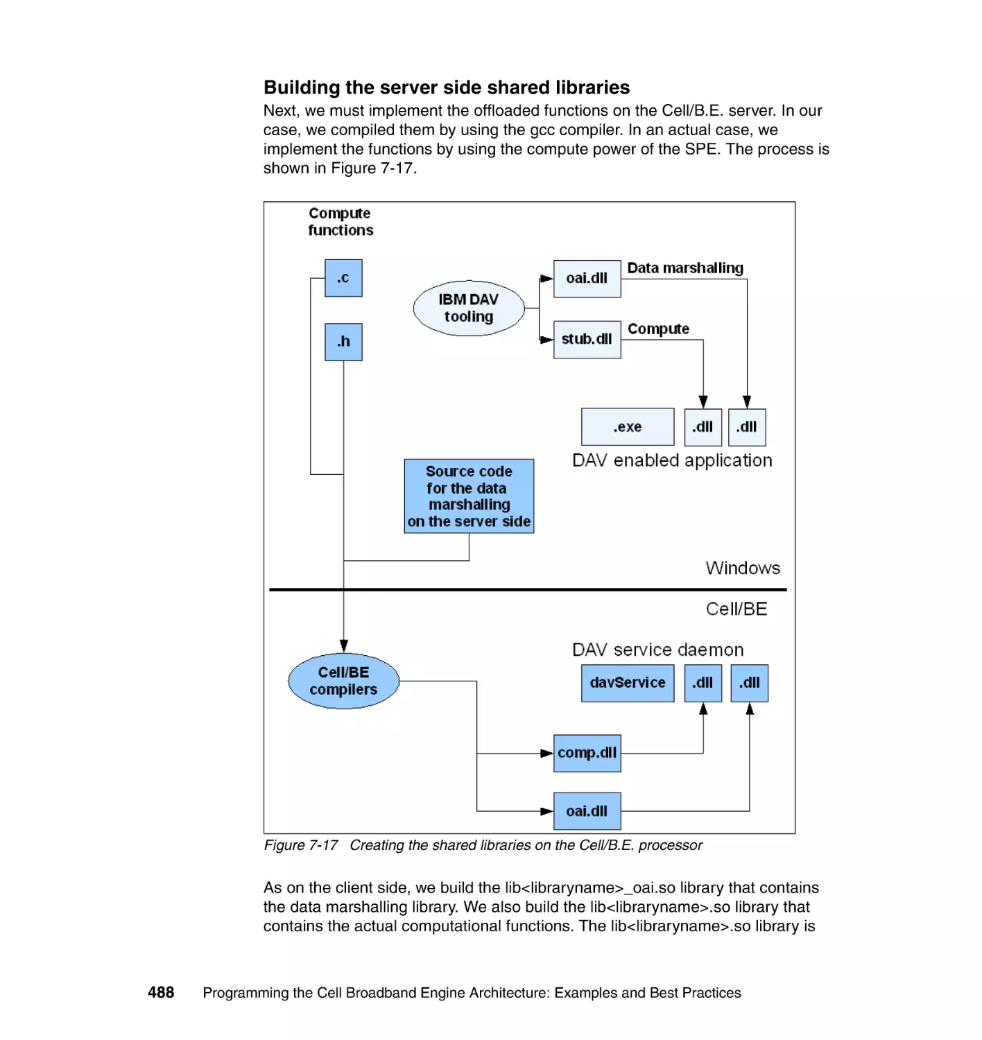


Автор: Arevalo A. Matinata R.M. Pandian M.
Теги: programming languages programming
ISBN: 0738485942
Год: 2008
Похожие


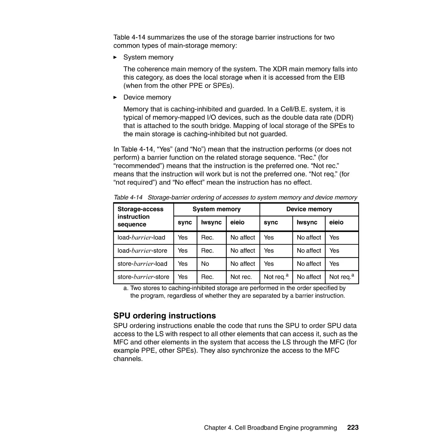
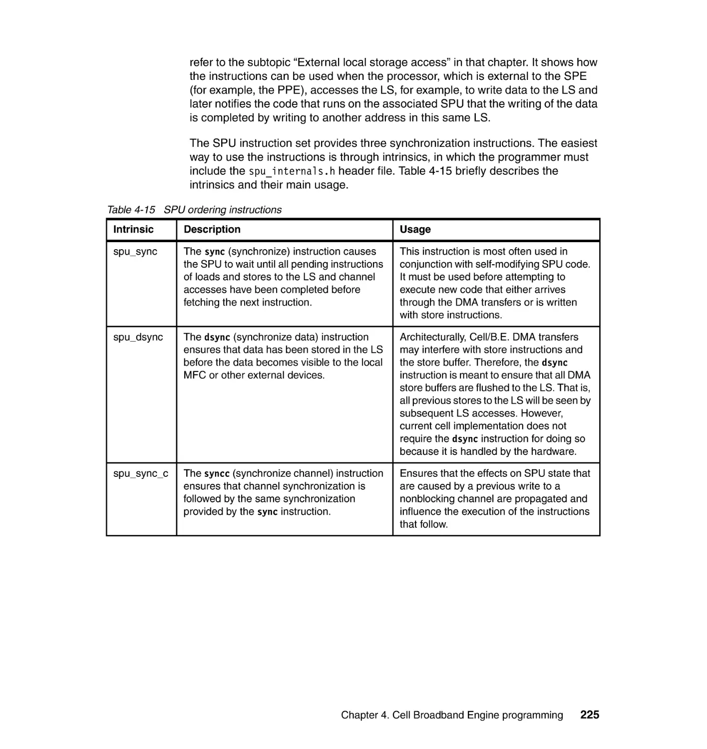
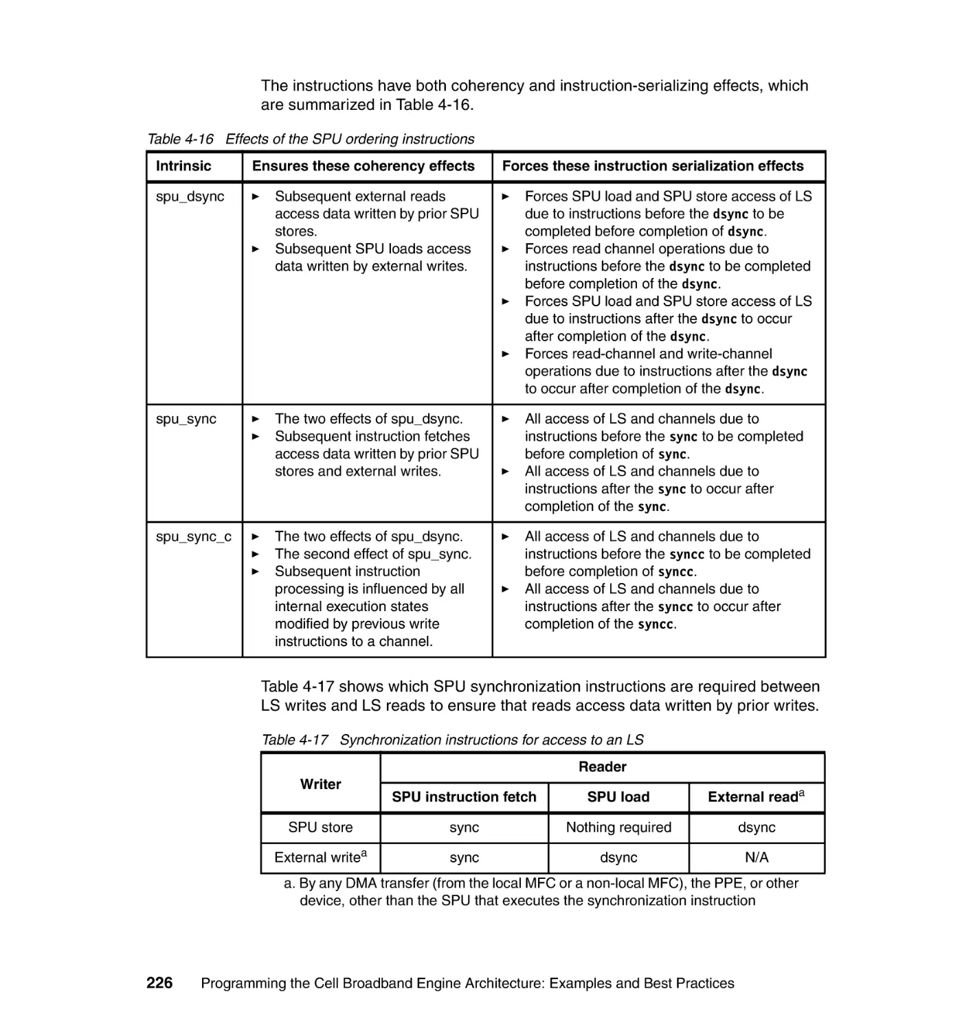
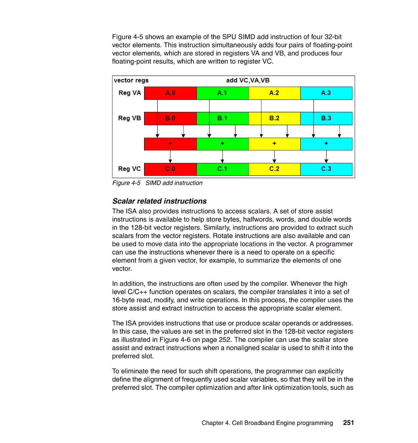
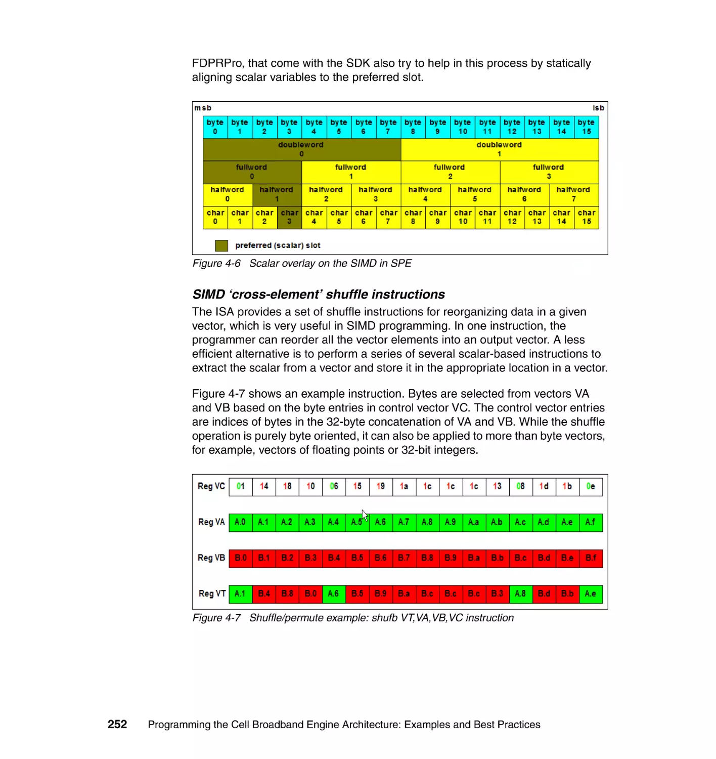
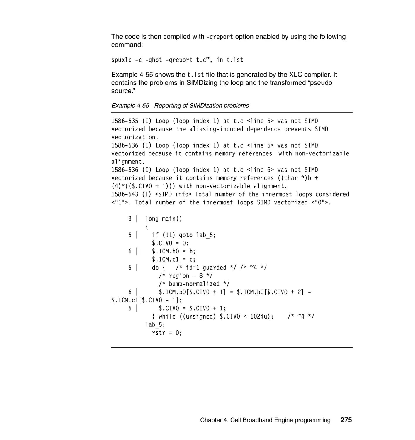
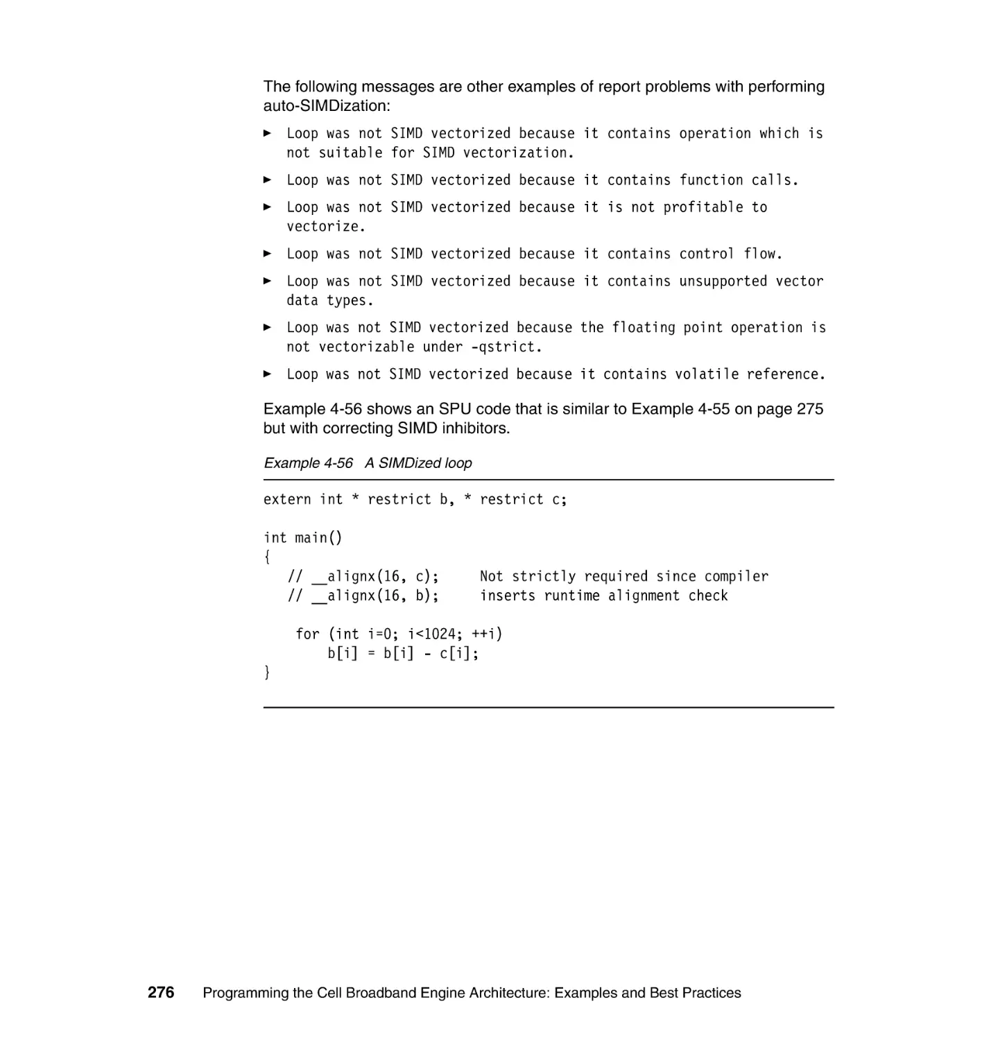
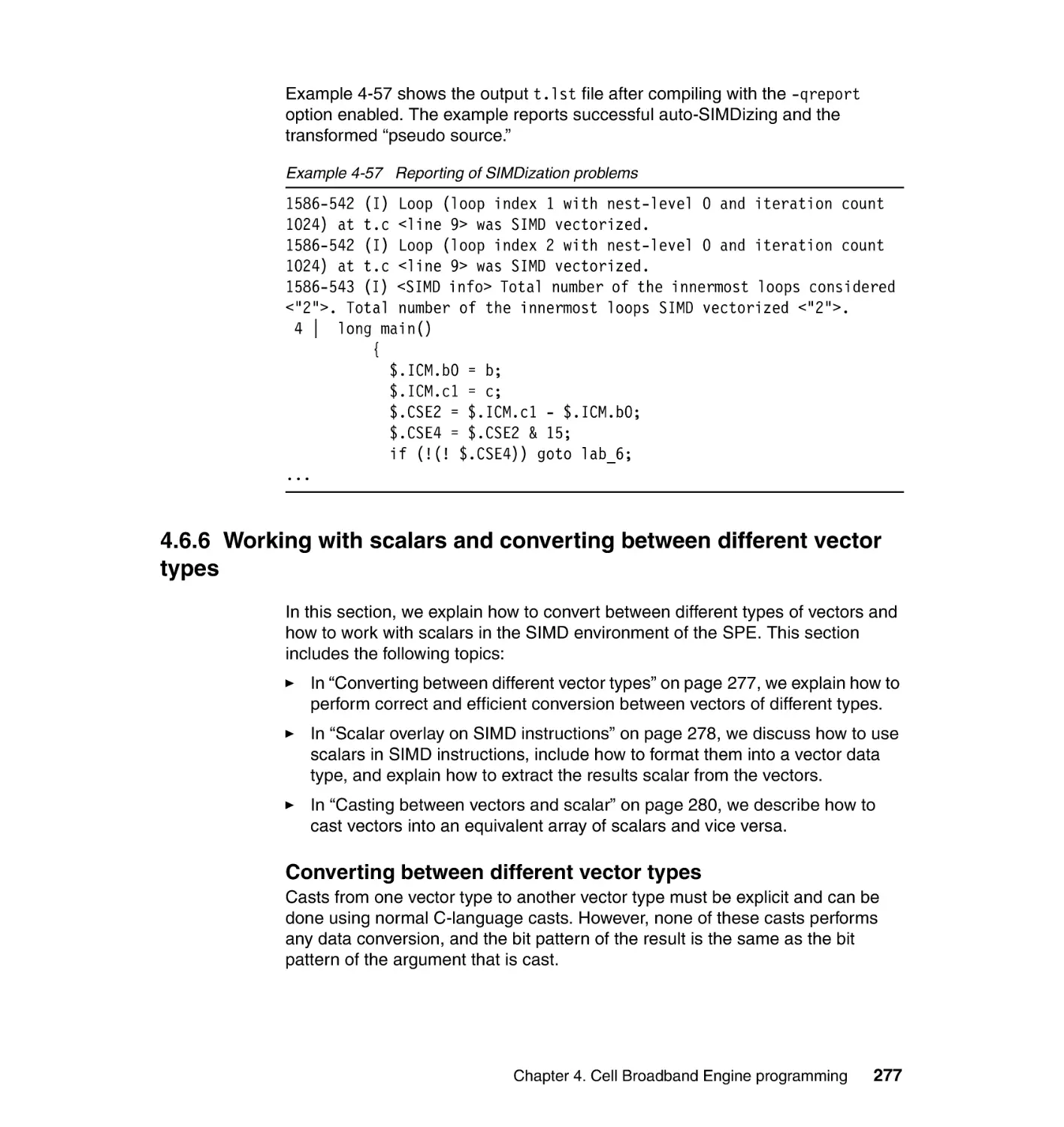
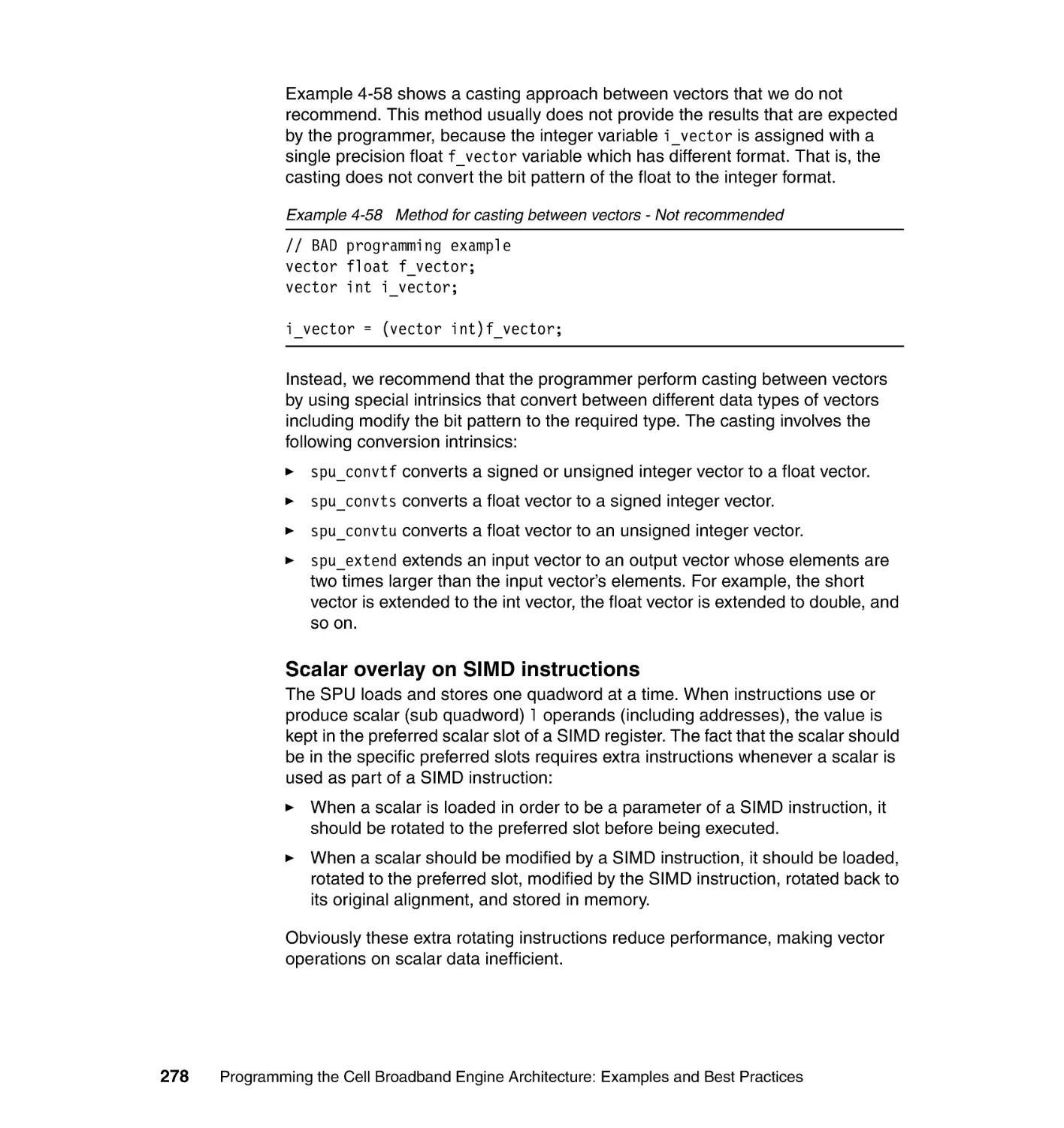
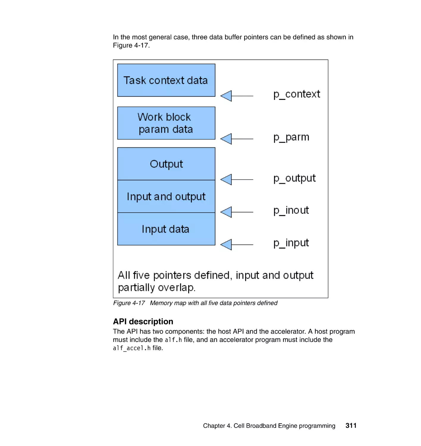
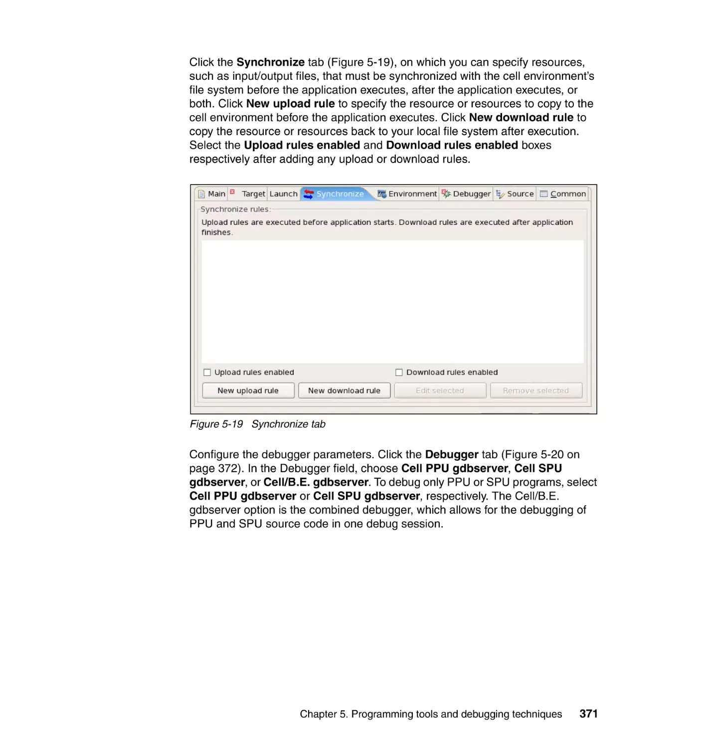
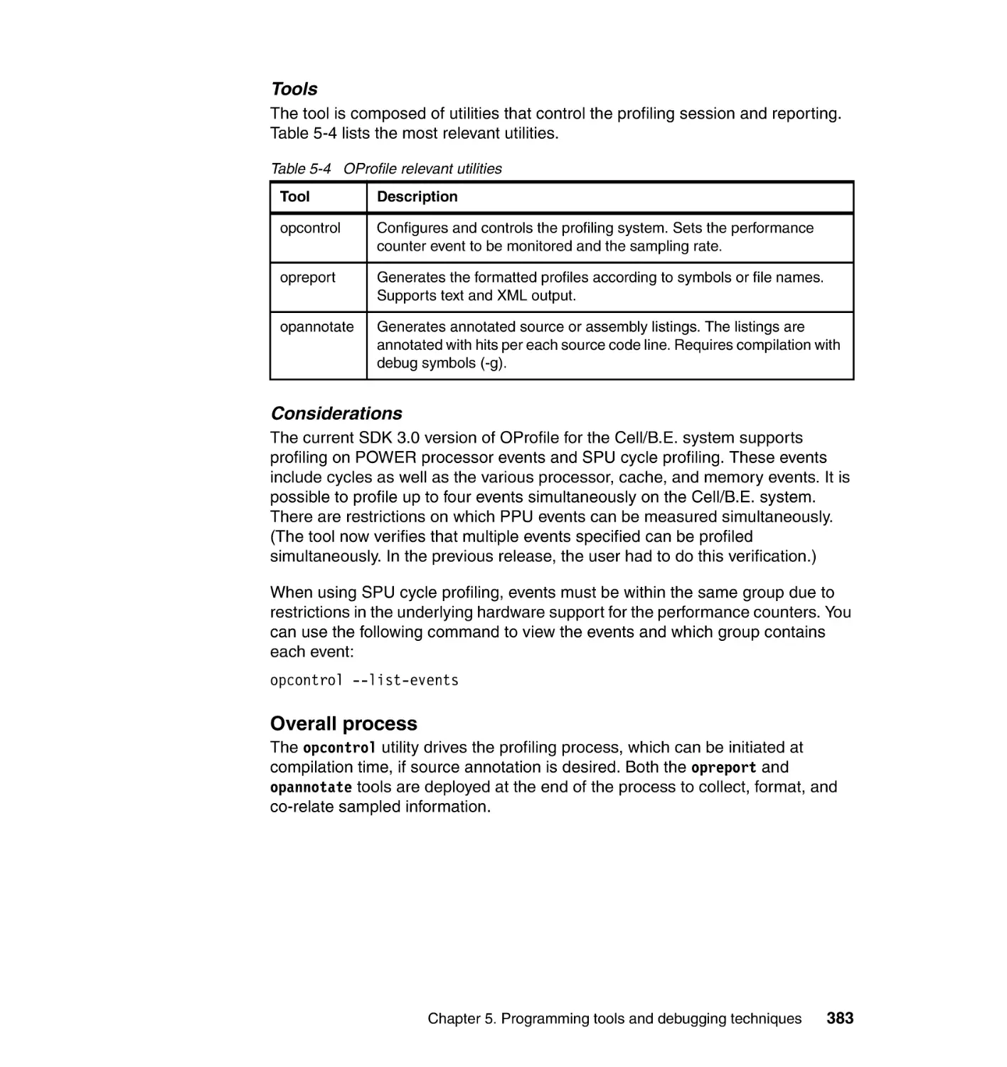
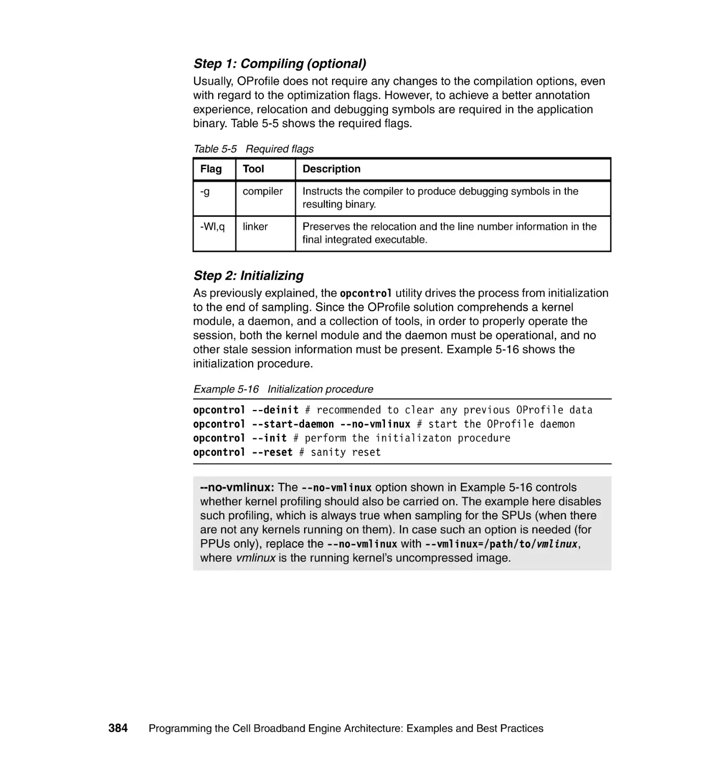
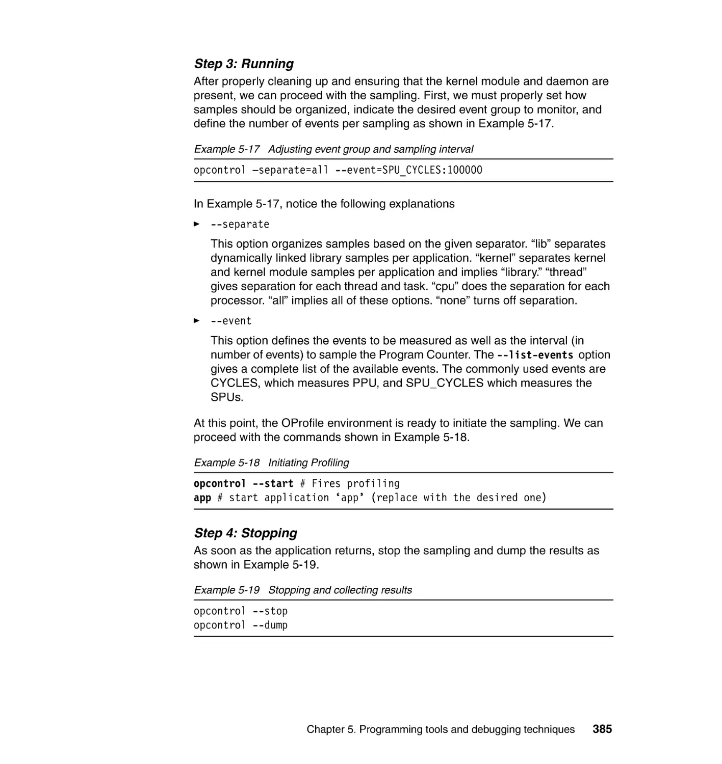
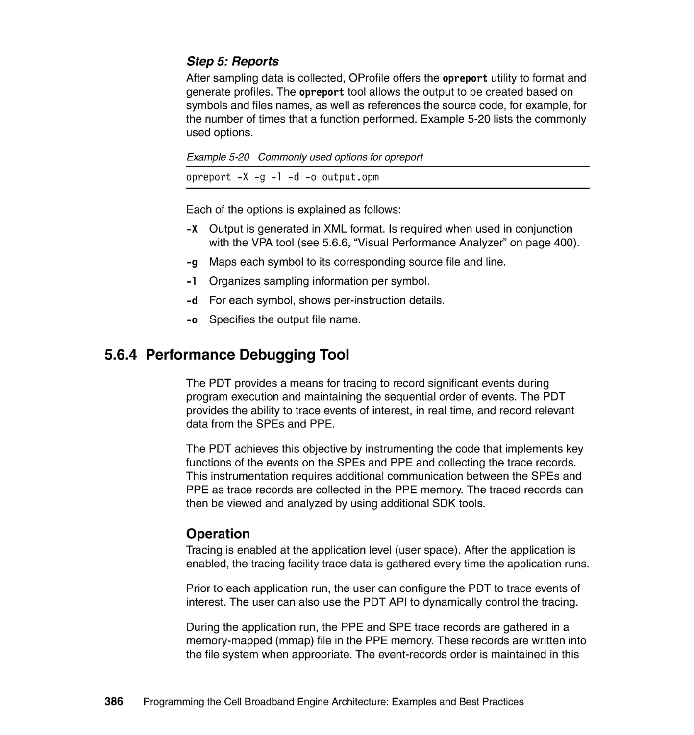
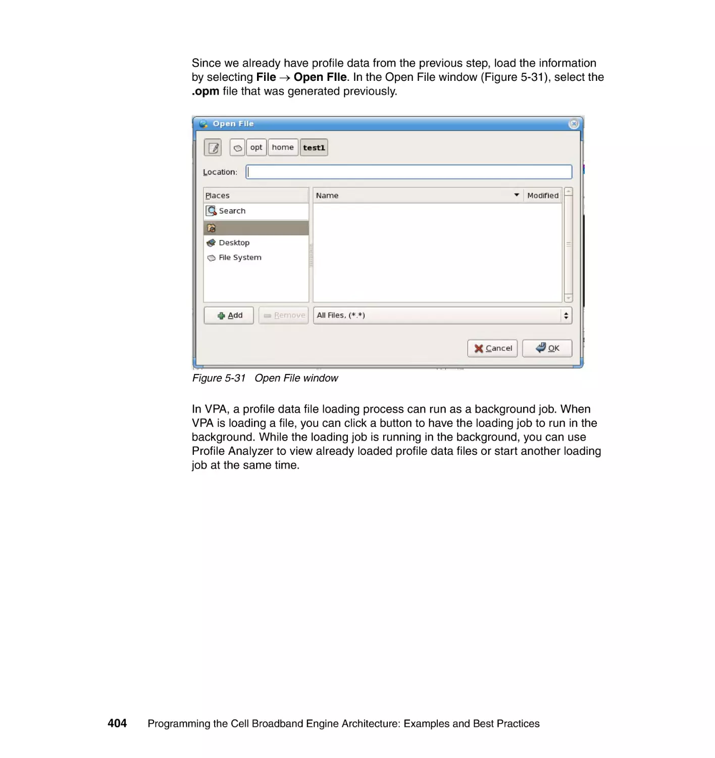
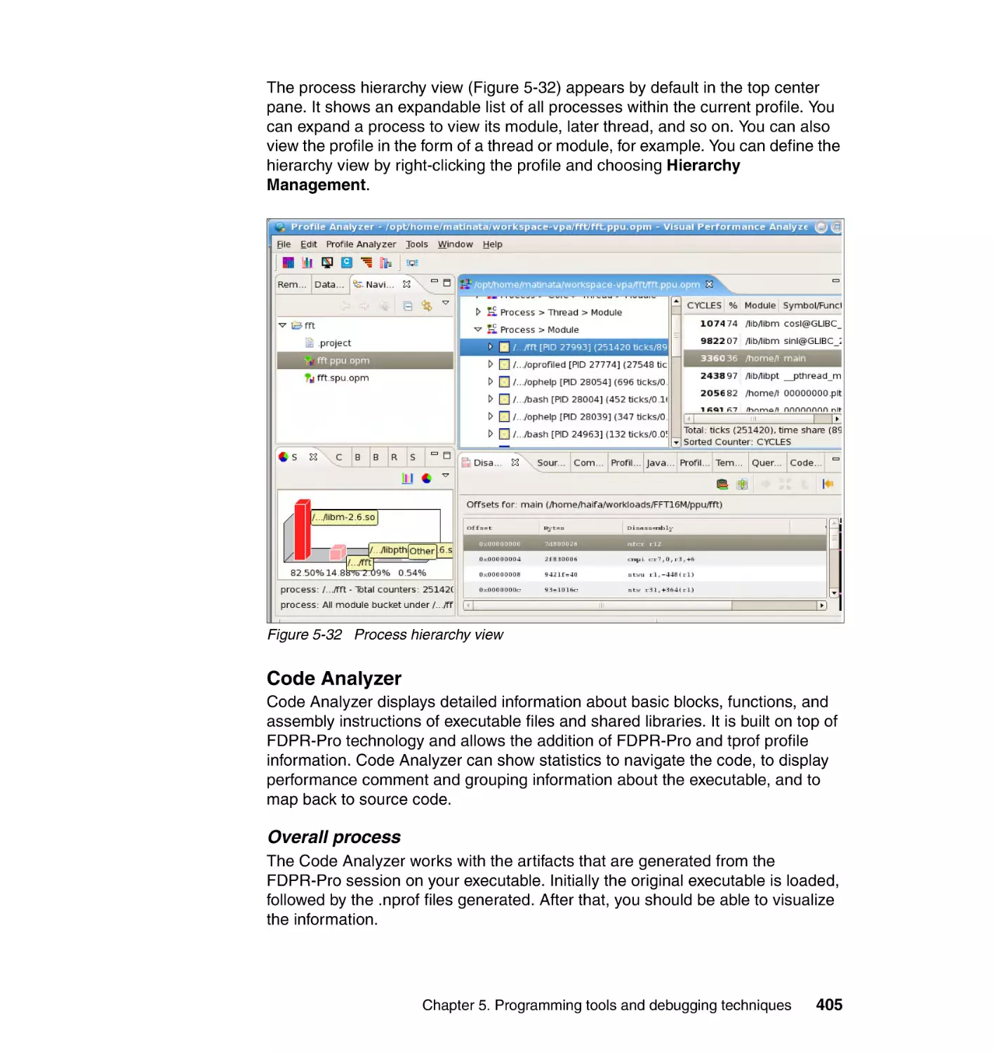
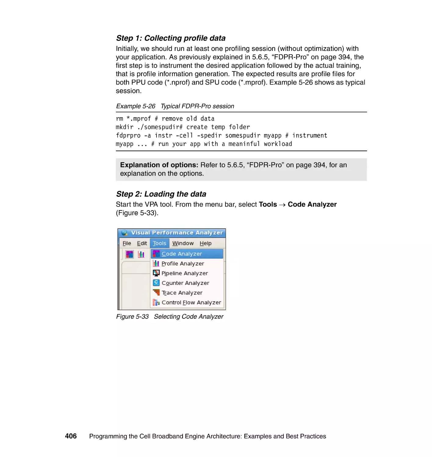
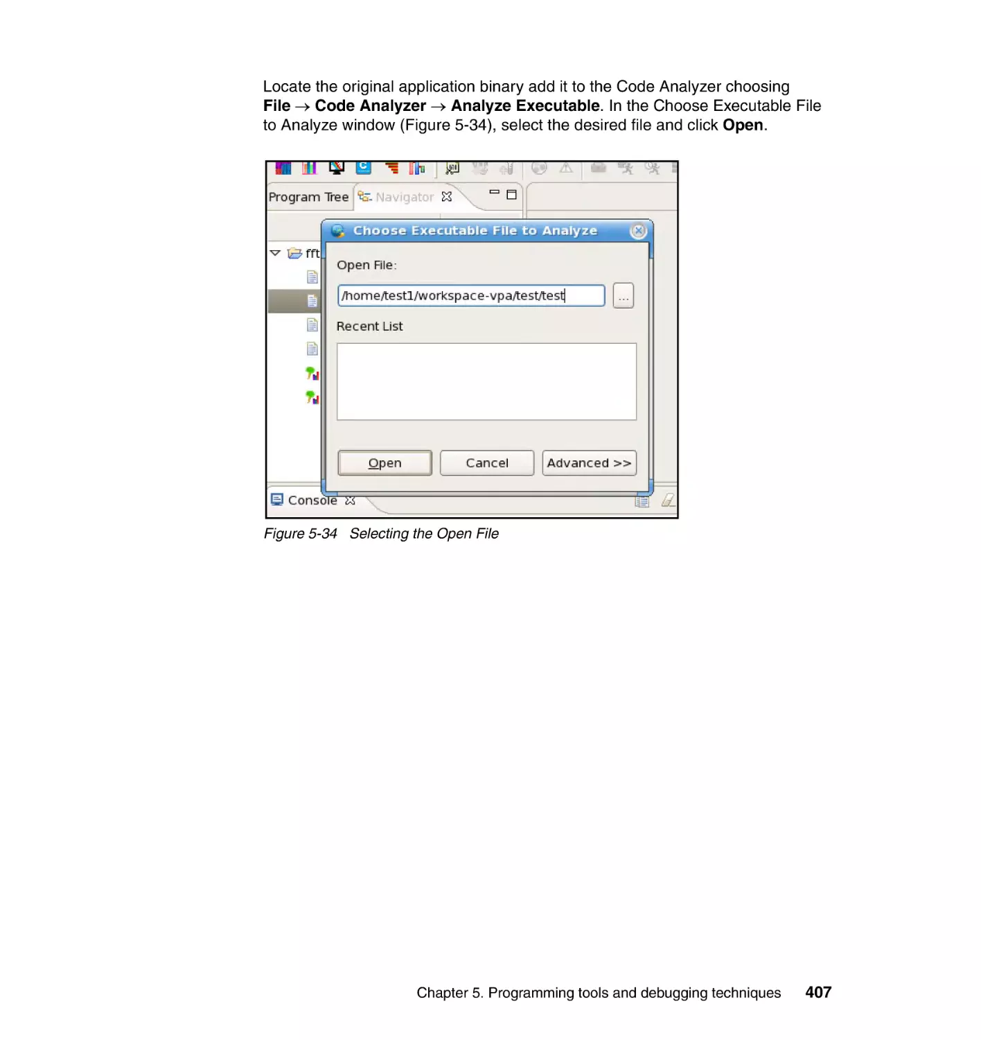
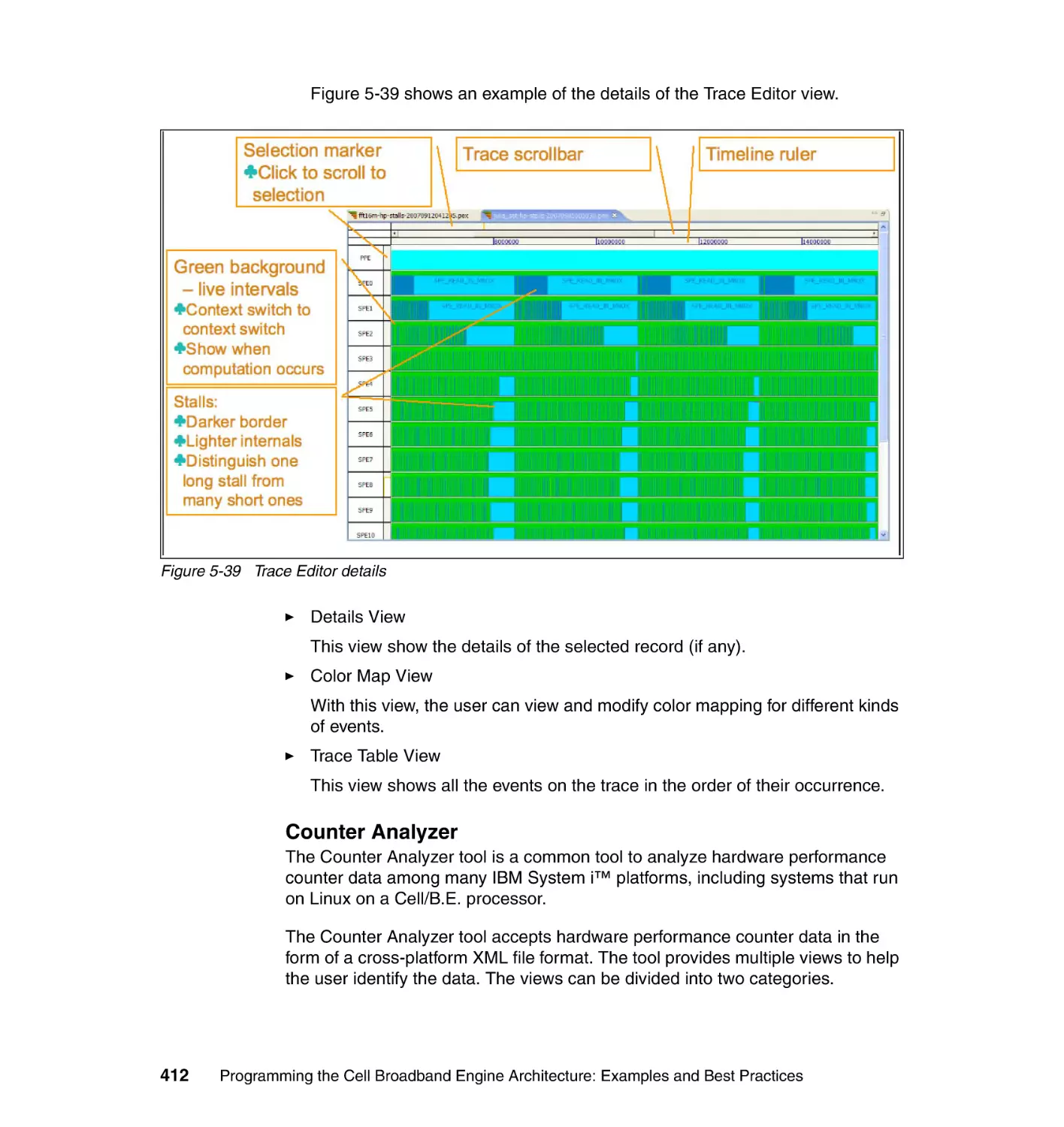
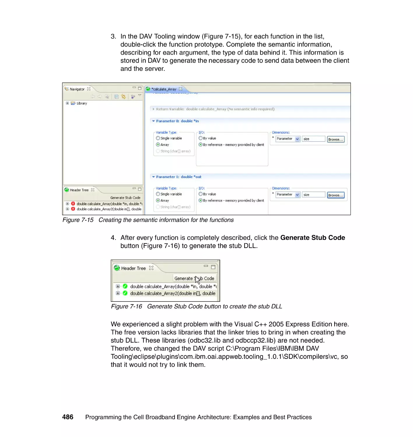
Текст
Front cover
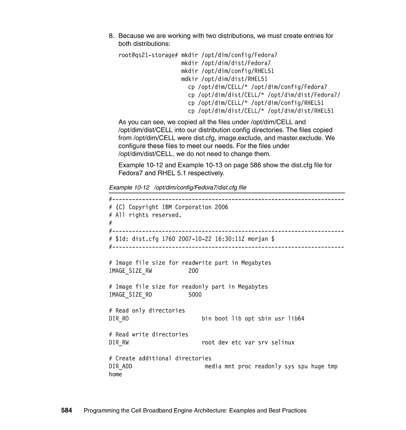
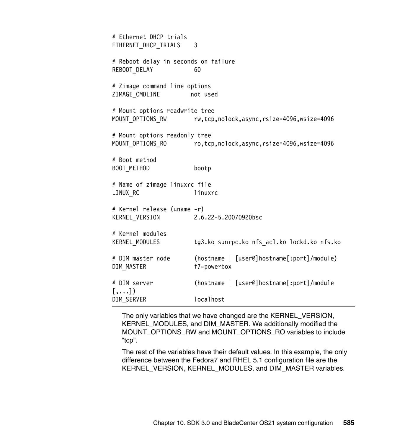
Programming the Cell Broadband
Engine™ Architecture
Examples and Best Practices
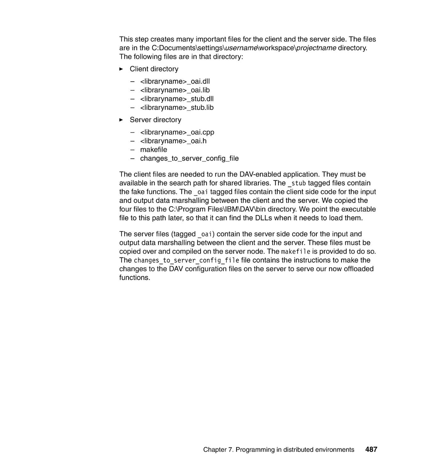
Understand and apply different
programming models and strategies
Make the most of SDK 3.0 debug
and performance tools
Use practical code development
and porting examples
Abraham Arevalo
Ricardo M. Matinata
Maharaja Pandian
Eitan Peri
Kurtis Ruby
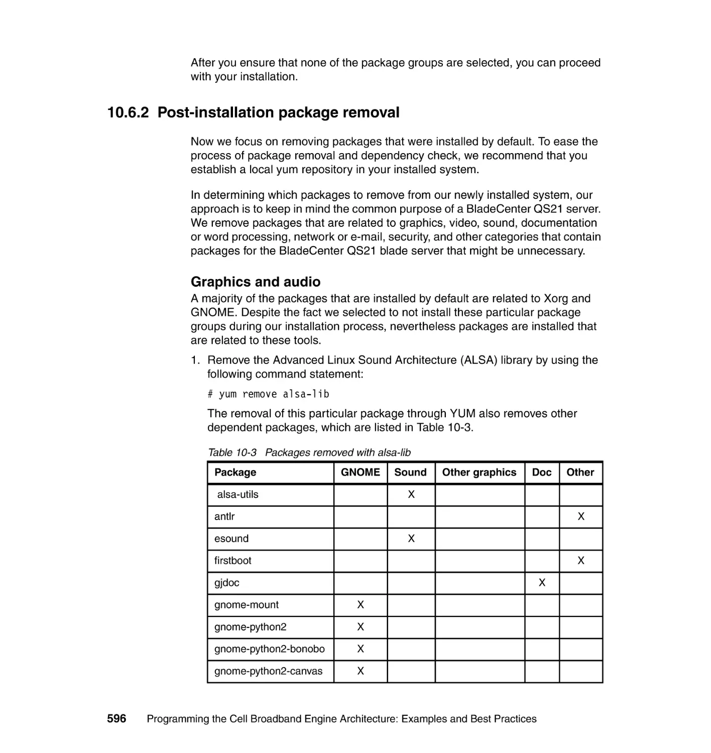
Francois Thomas
Chris Almond
ibm.com/redbooks
International Technical Support Organization
Programming the Cell Broadband Engine
Architecture: Examples and Best Practices
August 2008
SG24-7575-00
Note: Before using this information and the product it supports, read the information in
“Notices” on page xi.
First Edition (August 2008)
This edition applies to Version 3.0 of the IBM Cell Broadband Engine SDK, and the IBM
BladeCenter QS-21 platform.
© Copyright International Business Machines Corporation 2008. All rights reserved.
Note to U.S. Government Users Restricted Rights -- Use, duplication or disclosure restricted by GSA ADP
Schedule Contract with IBM Corp.
Contents
Notices . . . . . . . . . . . . . . . . . . . . . . . . . . . . . . . . . . . . . . . . . . . . . . . . . . . . . . . xi
Trademarks . . . . . . . . . . . . . . . . . . . . . . . . . . . . . . . . . . . . . . . . . . . . . . . . . . . xii
Preface . . . . . . . . . . . . . . . . . . . . . . . . . . . . . . . . . . . . . . . . . . . . . . . . . . . . . . xiii
The team that wrote this book . . . . . . . . . . . . . . . . . . . . . . . . . . . . . . . . . . . . . xiii
Acknowledgements . . . . . . . . . . . . . . . . . . . . . . . . . . . . . . . . . . . . . . . . . . . . . xv
Become a published author . . . . . . . . . . . . . . . . . . . . . . . . . . . . . . . . . . . . . . xvii
Comments welcome. . . . . . . . . . . . . . . . . . . . . . . . . . . . . . . . . . . . . . . . . . . . xvii
Part 1. Introduction to the Cell Broadband Engine Architecture . . . . . . . . . . . . . . . . . . . . . 1
Chapter 1. Cell Broadband Engine overview . . . . . . . . . . . . . . . . . . . . . . . . 3
1.1 Motivation . . . . . . . . . . . . . . . . . . . . . . . . . . . . . . . . . . . . . . . . . . . . . . . . . . 4
1.2 Scaling the three performance-limiting walls . . . . . . . . . . . . . . . . . . . . . . . . 6
1.2.1 Scaling the power-limitation wall . . . . . . . . . . . . . . . . . . . . . . . . . . . . . 6
1.2.2 Scaling the memory-limitation wall . . . . . . . . . . . . . . . . . . . . . . . . . . . 7
1.2.3 Scaling the frequency-limitation wall . . . . . . . . . . . . . . . . . . . . . . . . . . 7
1.2.4 How the Cell/B.E. processor overcomes performance limitations . . . 8
1.3 Hardware environment . . . . . . . . . . . . . . . . . . . . . . . . . . . . . . . . . . . . . . . . 8
1.3.1 The processor elements . . . . . . . . . . . . . . . . . . . . . . . . . . . . . . . . . . . 8
1.3.2 The element interconnect bus . . . . . . . . . . . . . . . . . . . . . . . . . . . . . . . 9
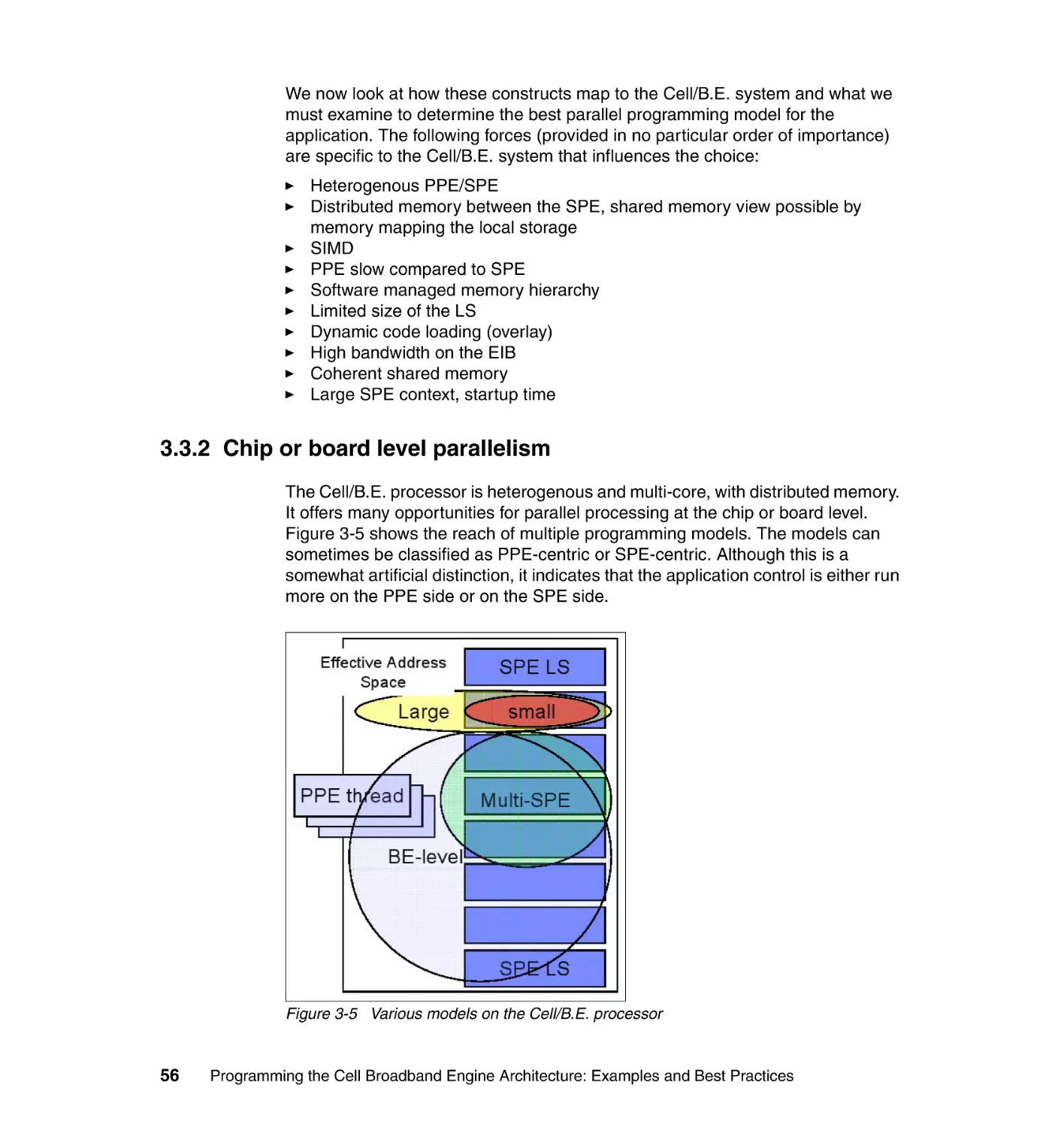
1.3.3 Memory interface controller. . . . . . . . . . . . . . . . . . . . . . . . . . . . . . . . 10
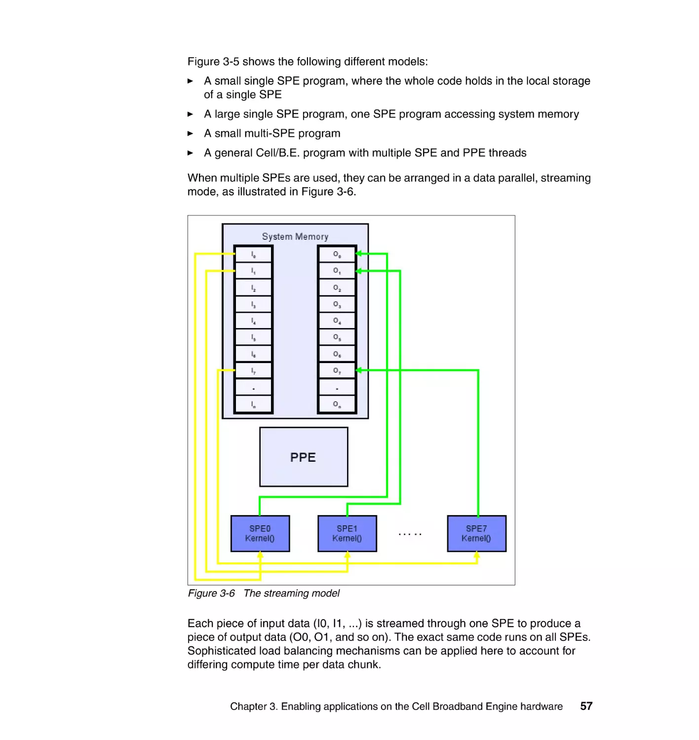
1.3.4 Cell Broadband Engine interface unit . . . . . . . . . . . . . . . . . . . . . . . . 10
1.4 Programming environment . . . . . . . . . . . . . . . . . . . . . . . . . . . . . . . . . . . . 11
1.4.1 Instruction sets . . . . . . . . . . . . . . . . . . . . . . . . . . . . . . . . . . . . . . . . . 11
1.4.2 Storage domains and interfaces . . . . . . . . . . . . . . . . . . . . . . . . . . . . 12
1.4.3 Bit ordering and numbering . . . . . . . . . . . . . . . . . . . . . . . . . . . . . . . . 14
1.4.4 Runtime environment . . . . . . . . . . . . . . . . . . . . . . . . . . . . . . . . . . . . 15
Chapter 2. IBM SDK for Multicore Acceleration . . . . . . . . . . . . . . . . . . . . . 17
2.1 Compilers . . . . . . . . . . . . . . . . . . . . . . . . . . . . . . . . . . . . . . . . . . . . . . . . . 18
2.1.1 GNU toolchain. . . . . . . . . . . . . . . . . . . . . . . . . . . . . . . . . . . . . . . . . . 18
2.1.2 IBM XLC/C++ compiler . . . . . . . . . . . . . . . . . . . . . . . . . . . . . . . . . . . 18
2.1.3 GNU ADA compiler . . . . . . . . . . . . . . . . . . . . . . . . . . . . . . . . . . . . . . 18
2.1.4 IBM XL Fortran for Multicore Acceleration for Linux . . . . . . . . . . . . . 19
2.2 IBM Full System Simulator . . . . . . . . . . . . . . . . . . . . . . . . . . . . . . . . . . . . 19
2.2.1 System root image for the simulator . . . . . . . . . . . . . . . . . . . . . . . . . 20
© Copyright IBM Corp. 2008. All rights reserved.
iii
2.3 Linux kernel . . . . . . . . . . . . . . . . . . . . . . . . . . . . . . . . . . . . . . . . . . . . . . . . 20
2.4 Cell/B.E. libraries. . . . . . . . . . . . . . . . . . . . . . . . . . . . . . . . . . . . . . . . . . . . 21
2.4.1 SPE Runtime Management Library. . . . . . . . . . . . . . . . . . . . . . . . . . 21
2.4.2 SIMD Math Library . . . . . . . . . . . . . . . . . . . . . . . . . . . . . . . . . . . . . . 21
2.4.3 Mathematical Acceleration Subsystem libraries . . . . . . . . . . . . . . . . 21
2.4.4 Basic Linear Algebra Subprograms . . . . . . . . . . . . . . . . . . . . . . . . . 22
2.4.5 ALF library. . . . . . . . . . . . . . . . . . . . . . . . . . . . . . . . . . . . . . . . . . . . . 22
2.4.6 Data Communication and Synchronization library . . . . . . . . . . . . . . 23
2.5 Code examples and example libraries . . . . . . . . . . . . . . . . . . . . . . . . . . . 23
2.6 Performance tools . . . . . . . . . . . . . . . . . . . . . . . . . . . . . . . . . . . . . . . . . . . 24
2.6.1 SPU timing tool . . . . . . . . . . . . . . . . . . . . . . . . . . . . . . . . . . . . . . . . . 24
2.6.2 OProfile . . . . . . . . . . . . . . . . . . . . . . . . . . . . . . . . . . . . . . . . . . . . . . . 24
2.6.3 Cell-perf-counter tool. . . . . . . . . . . . . . . . . . . . . . . . . . . . . . . . . . . . . 24
2.6.4 Performance Debug Tool . . . . . . . . . . . . . . . . . . . . . . . . . . . . . . . . . 25
2.6.5 Feedback Directed Program Restructuring tool . . . . . . . . . . . . . . . . 25
2.6.6 Visual Performance Analyzer . . . . . . . . . . . . . . . . . . . . . . . . . . . . . . 25
2.7 IBM Eclipse IDE for the SDK. . . . . . . . . . . . . . . . . . . . . . . . . . . . . . . . . . . 26
2.8 Hybrid-x86 programming model . . . . . . . . . . . . . . . . . . . . . . . . . . . . . . . . 26
Part 2. Programming environment . . . . . . . . . . . . . . . . . . . . . . . . . . . . . . . . . . . . . . . . . . . . 29
Chapter 3. Enabling applications on the Cell Broadband Engine
hardware . . . . . . . . . . . . . . . . . . . . . . . . . . . . . . . . . . . . . . . . . . . 31
3.1 Concepts and terminology. . . . . . . . . . . . . . . . . . . . . . . . . . . . . . . . . . . . . 33
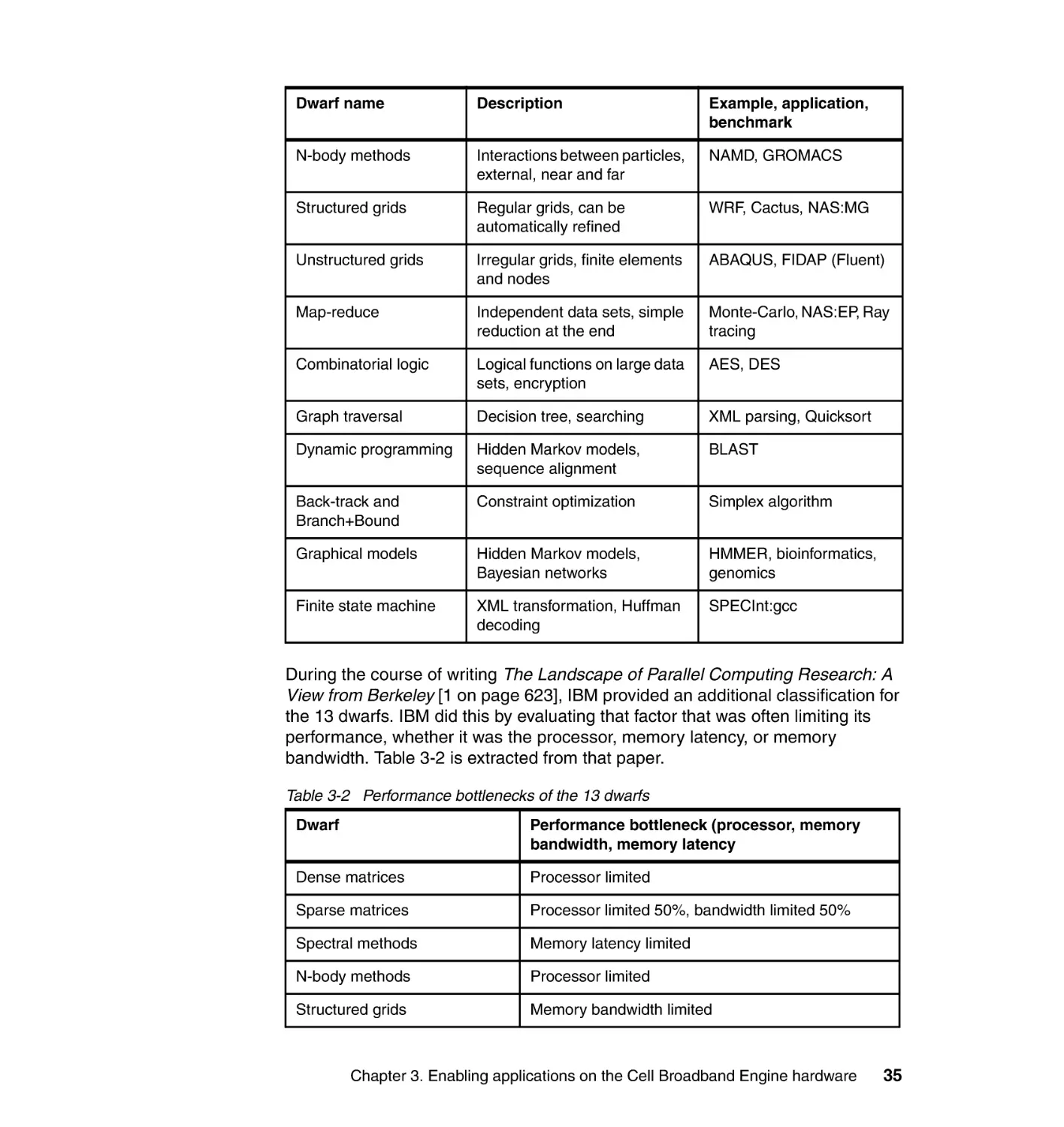
3.1.1 The computation kernels. . . . . . . . . . . . . . . . . . . . . . . . . . . . . . . . . . 34
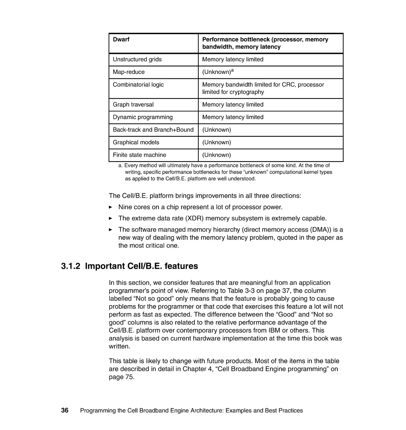
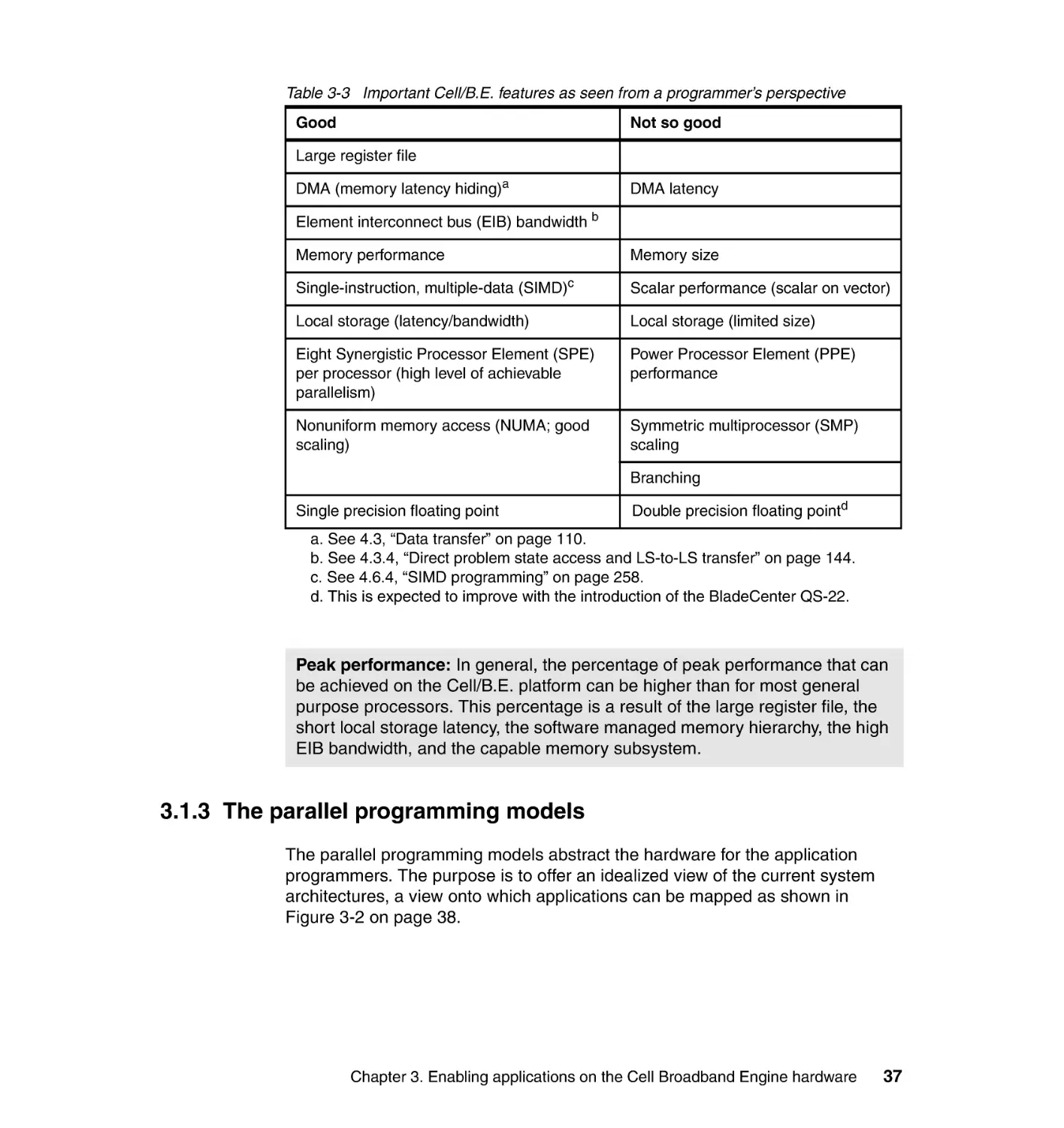
3.1.2 Important Cell/B.E. features . . . . . . . . . . . . . . . . . . . . . . . . . . . . . . . 36
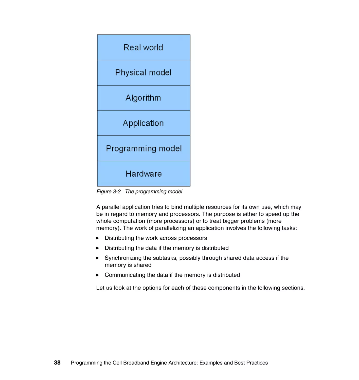
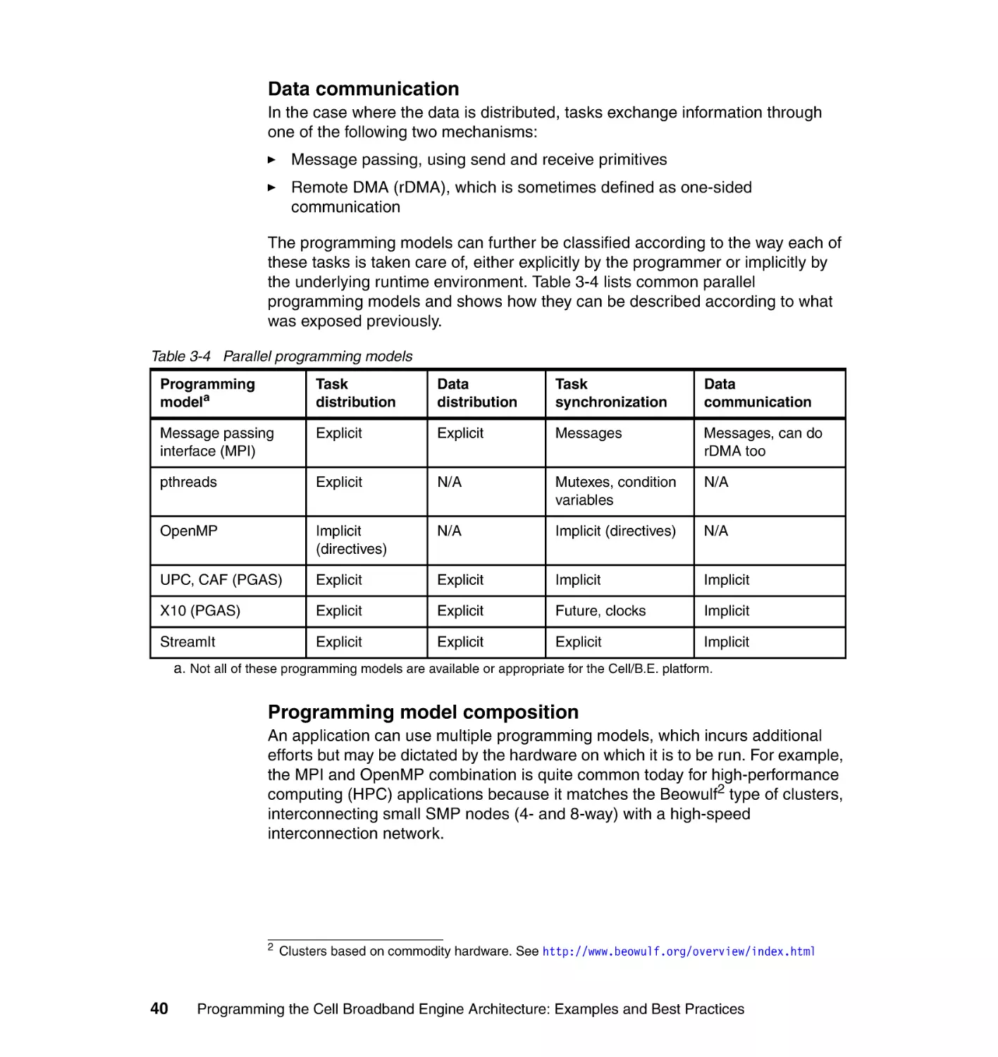
3.1.3 The parallel programming models. . . . . . . . . . . . . . . . . . . . . . . . . . . 37
3.1.4 The Cell/B.E. programming frameworks . . . . . . . . . . . . . . . . . . . . . . 41
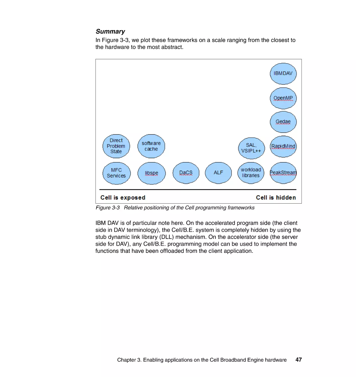
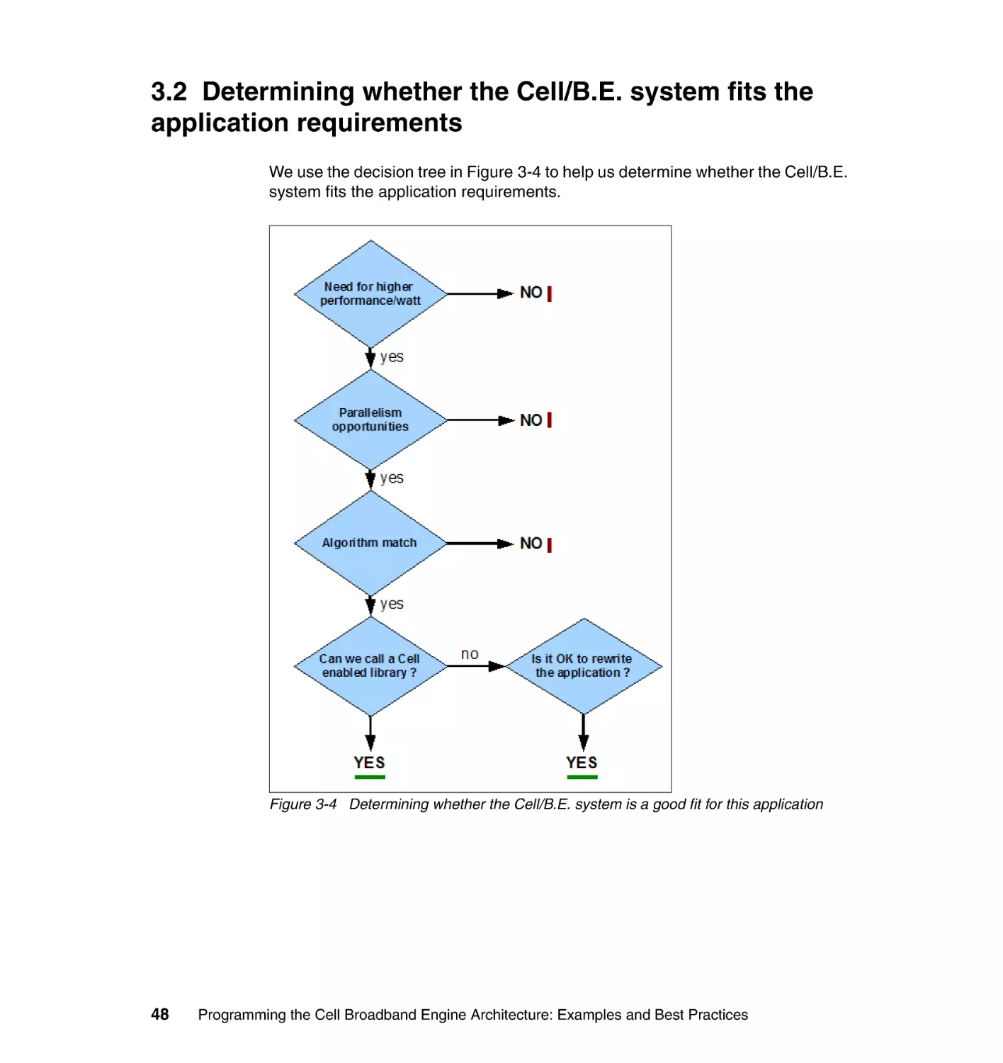
3.2 Determining whether the Cell/B.E. system fits the
application requirements . . . . . . . . . . . . . . . . . . . . . . . . . . . . . . . . . . . . . 48
3.2.1 Higher performance/watt . . . . . . . . . . . . . . . . . . . . . . . . . . . . . . . . . . 49
3.2.2 Opportunities for parallelism . . . . . . . . . . . . . . . . . . . . . . . . . . . . . . . 49
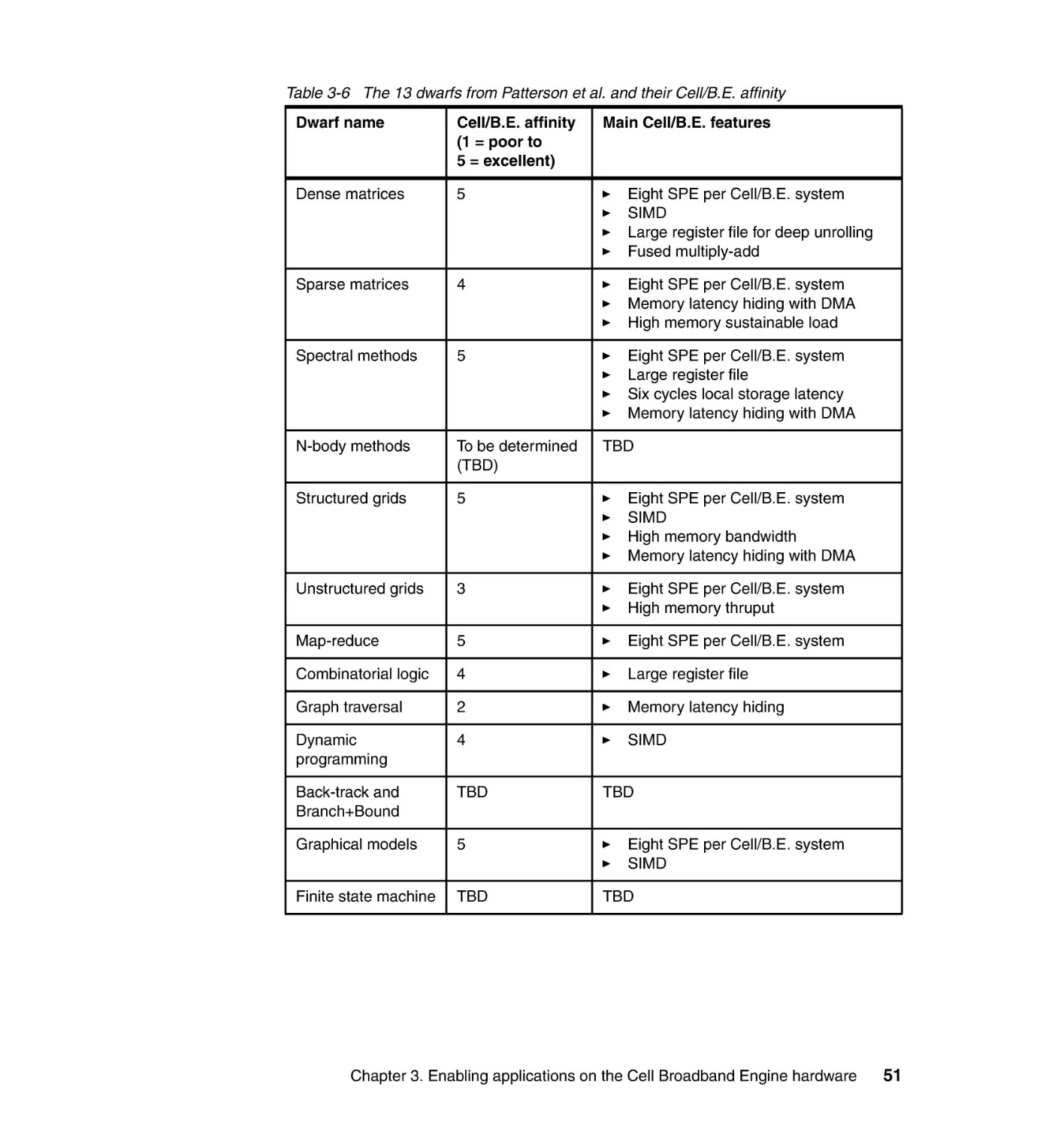
3.2.3 Algorithm match . . . . . . . . . . . . . . . . . . . . . . . . . . . . . . . . . . . . . . . . 50
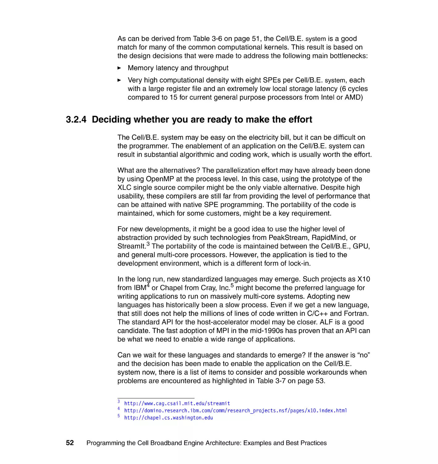
3.2.4 Deciding whether you are ready to make the effort . . . . . . . . . . . . . 52
3.3 Deciding which parallel programming model to use . . . . . . . . . . . . . . . . . 53
3.3.1 Parallel programming models basics . . . . . . . . . . . . . . . . . . . . . . . . 54
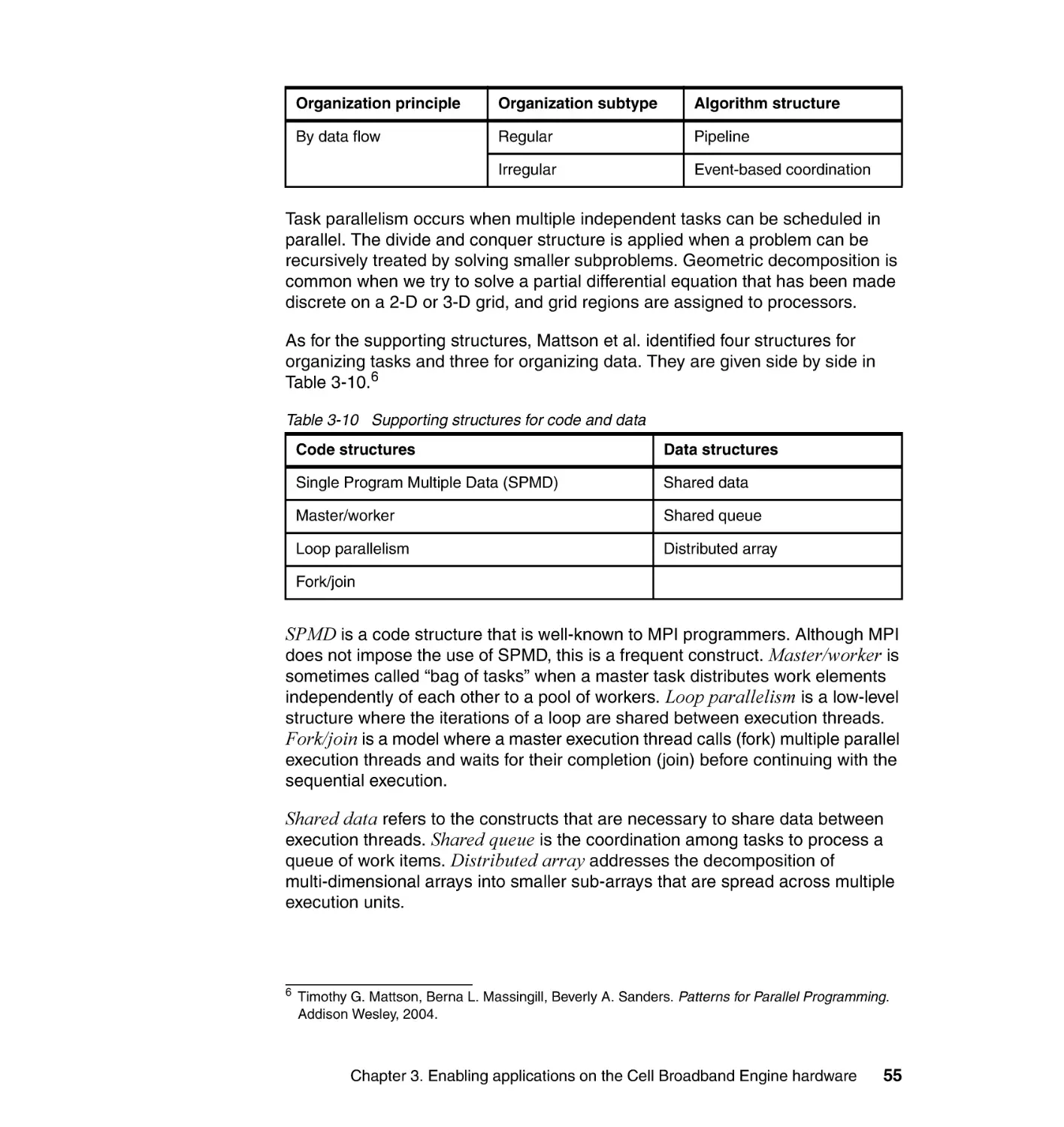
3.3.2 Chip or board level parallelism . . . . . . . . . . . . . . . . . . . . . . . . . . . . . 56
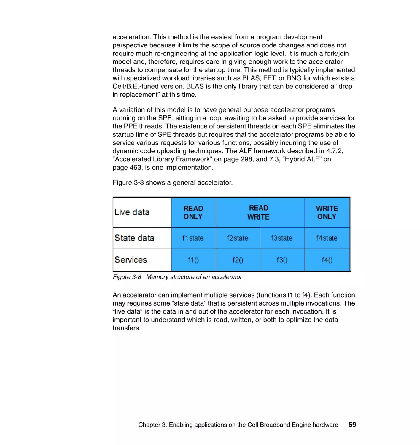
3.3.3 More on the host-accelerator model . . . . . . . . . . . . . . . . . . . . . . . . . 58
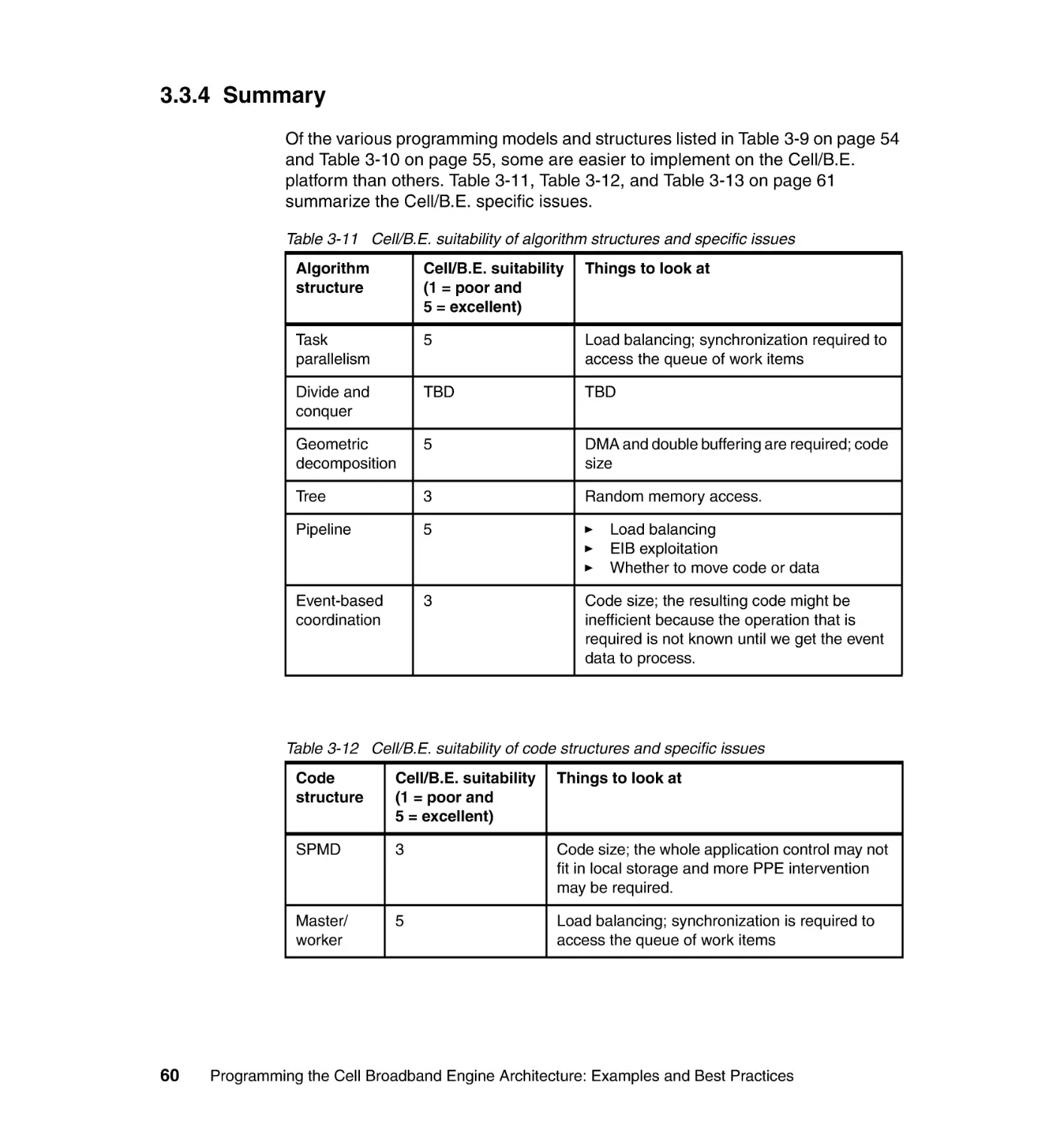
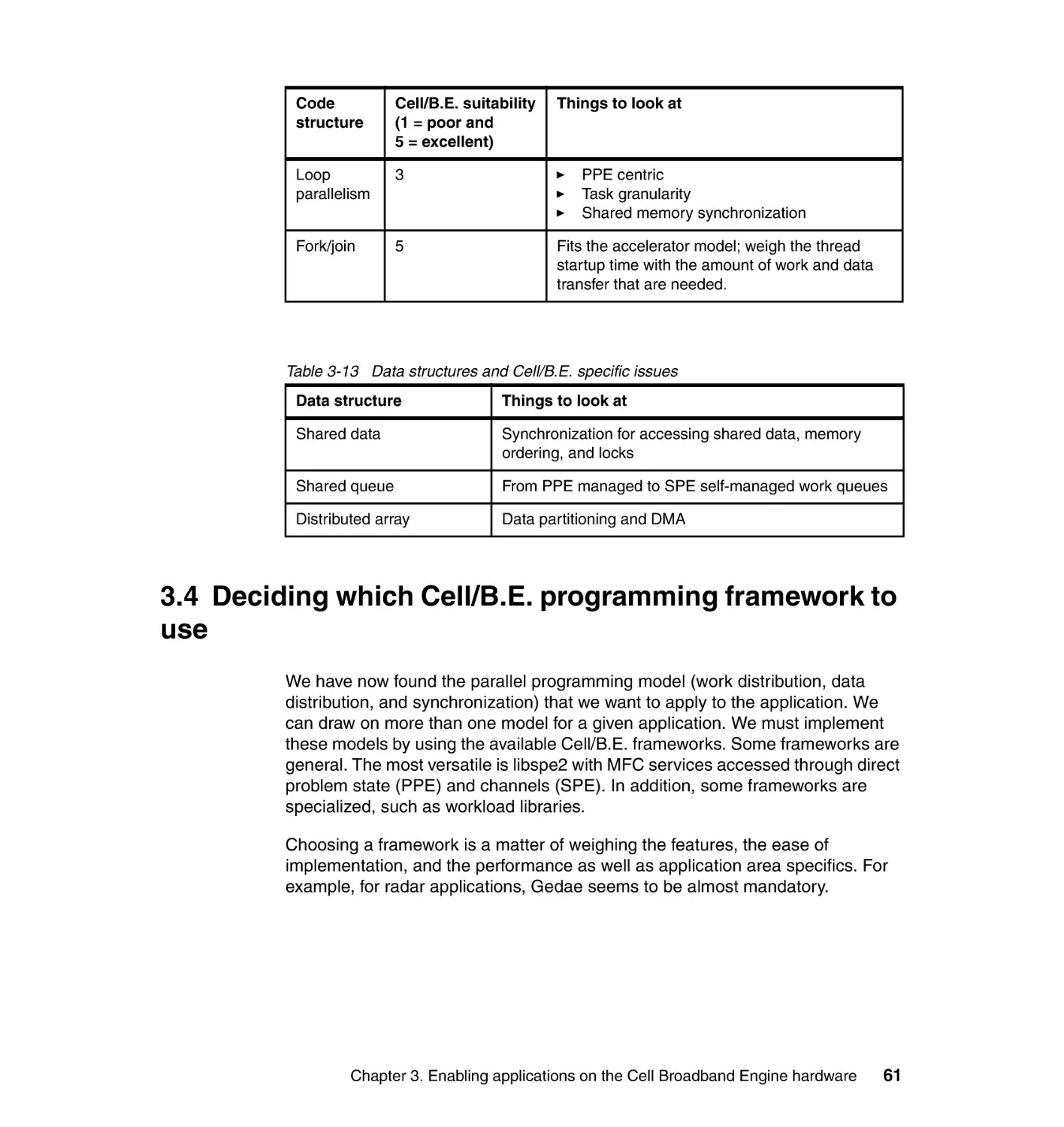
3.3.4 Summary . . . . . . . . . . . . . . . . . . . . . . . . . . . . . . . . . . . . . . . . . . . . . . 60
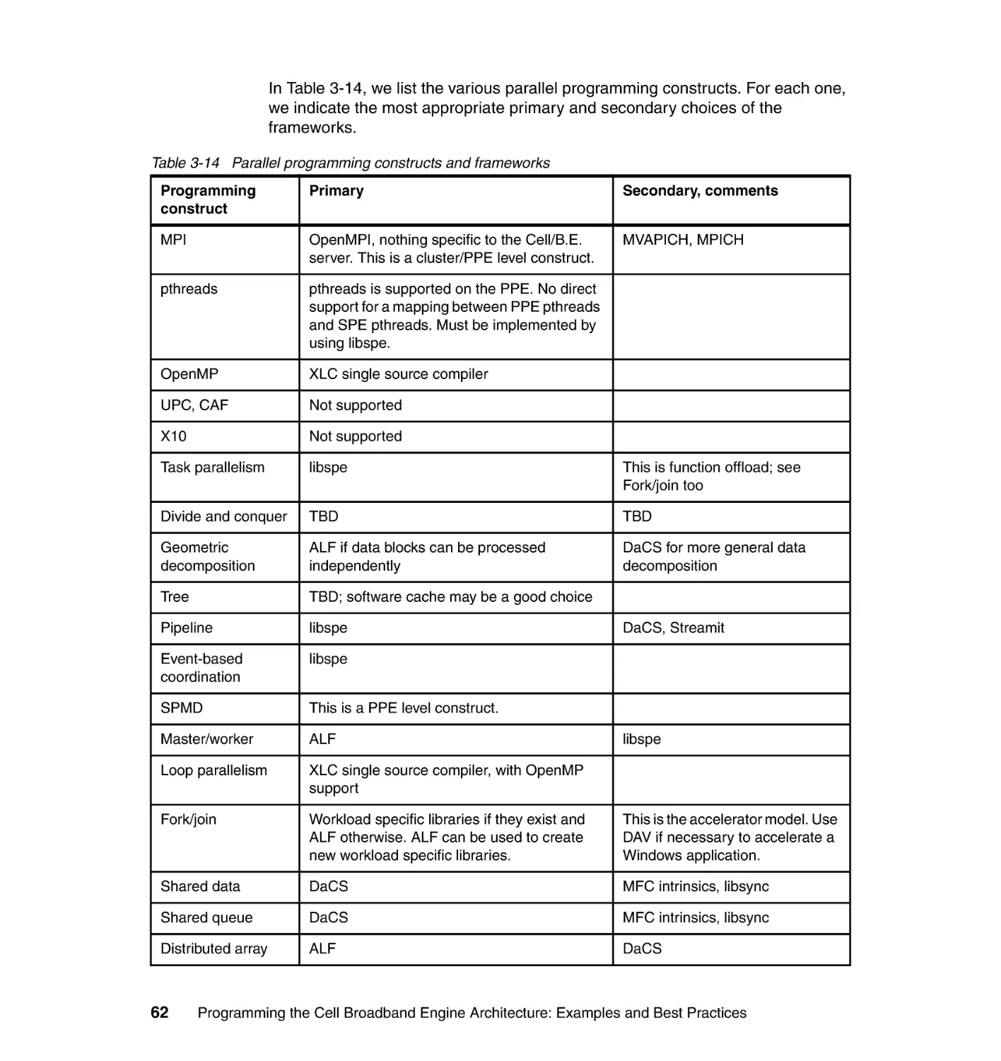
3.4 Deciding which Cell/B.E. programming framework to use . . . . . . . . . . . . 61
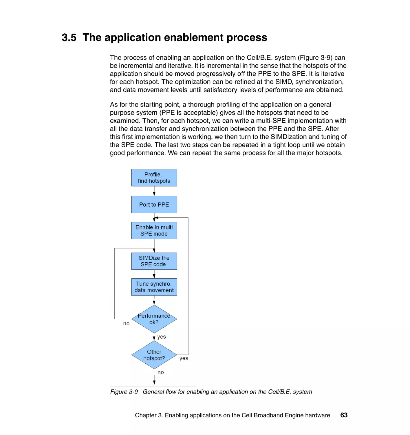
3.5 The application enablement process. . . . . . . . . . . . . . . . . . . . . . . . . . . . . 63
3.5.1 Performance tuning for Cell/B.E. programs . . . . . . . . . . . . . . . . . . . 66
iv
Programming the Cell Broadband Engine Architecture: Examples and Best Practices
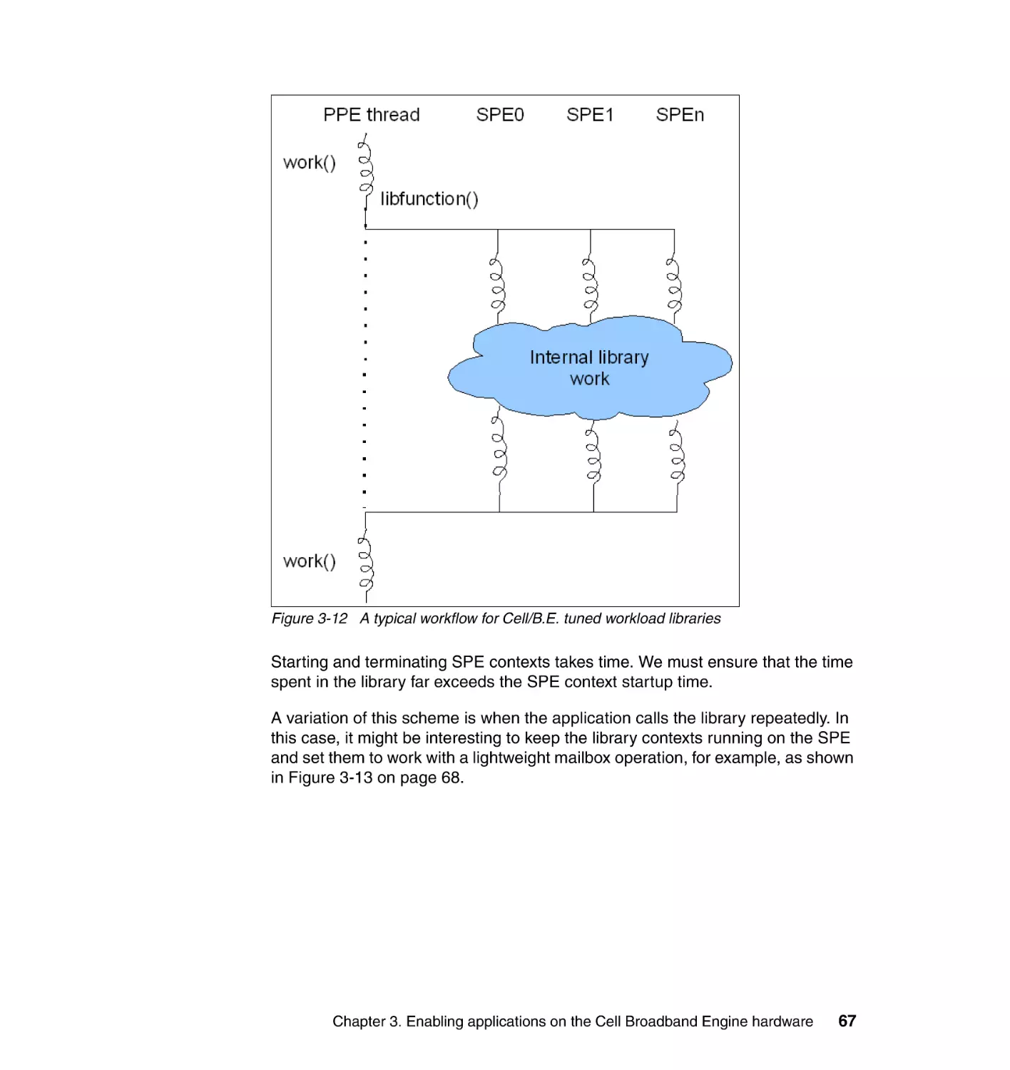
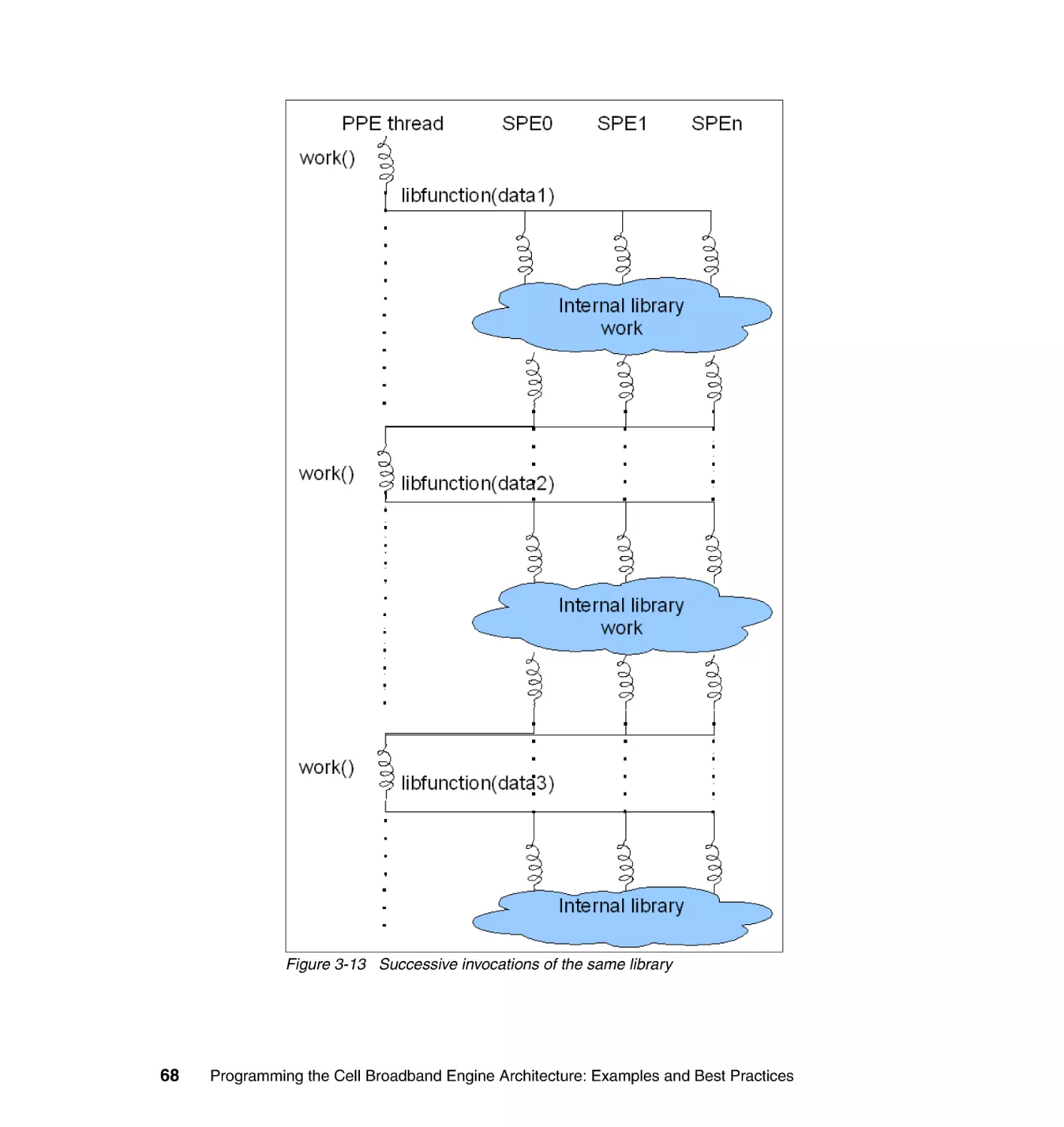
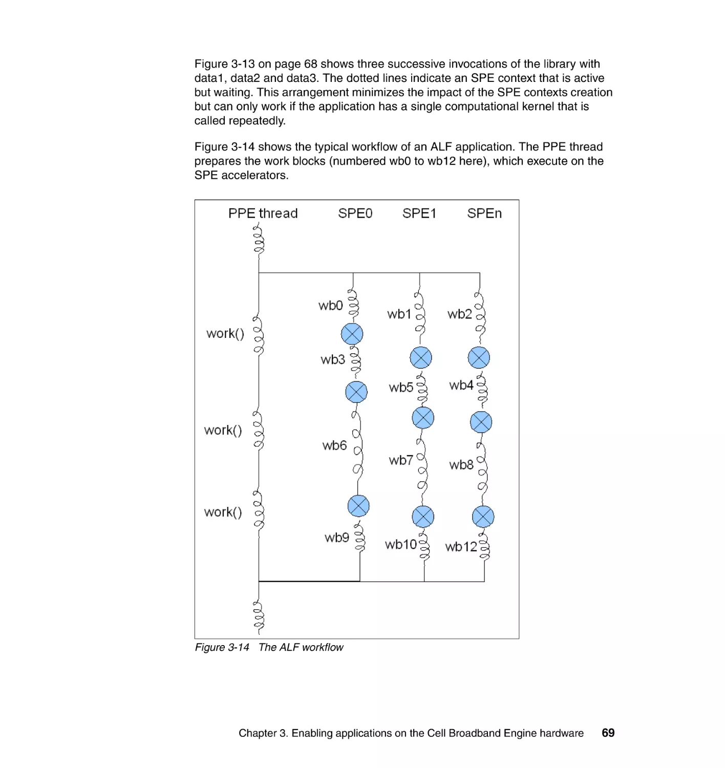
3.6 A few scenarios . . . . . . . . . . . . . . . . . . . . . . . . . . . . . . . . . . . . . . . . . . . . . 66
3.7 Design patterns for Cell/B.E. programming . . . . . . . . . . . . . . . . . . . . . . . . 70
3.7.1 Shared queue . . . . . . . . . . . . . . . . . . . . . . . . . . . . . . . . . . . . . . . . . . 70
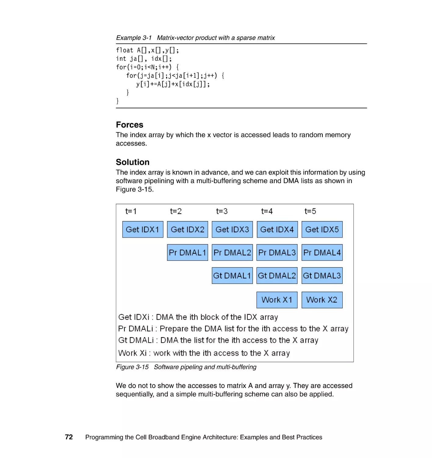
3.7.2 Indirect addressing . . . . . . . . . . . . . . . . . . . . . . . . . . . . . . . . . . . . . . 71
3.7.3 Pipeline . . . . . . . . . . . . . . . . . . . . . . . . . . . . . . . . . . . . . . . . . . . . . . . 73
3.7.4 Multi-SPE software cache . . . . . . . . . . . . . . . . . . . . . . . . . . . . . . . . . 73
3.7.5 Plug-in . . . . . . . . . . . . . . . . . . . . . . . . . . . . . . . . . . . . . . . . . . . . . . . . 74
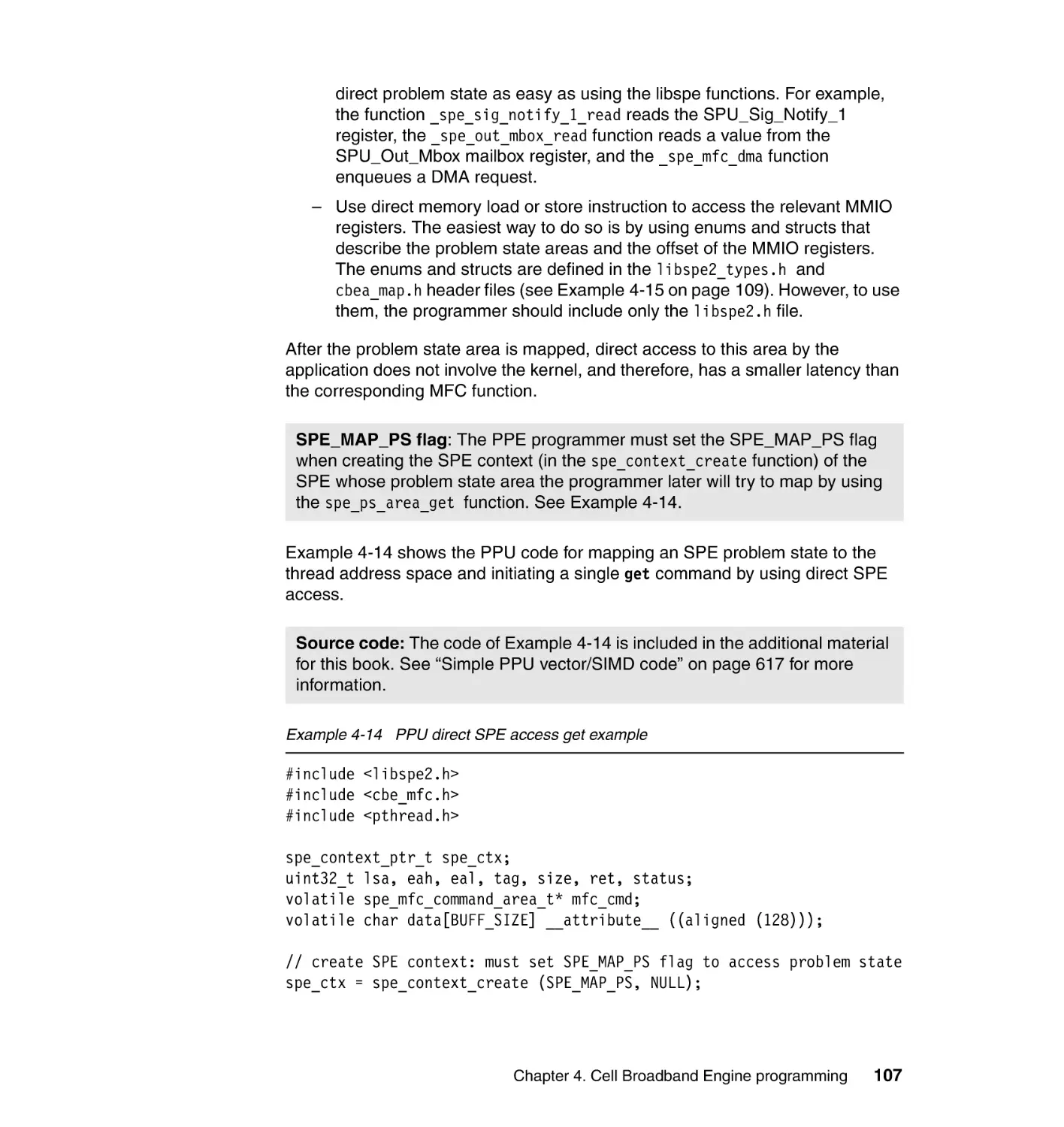
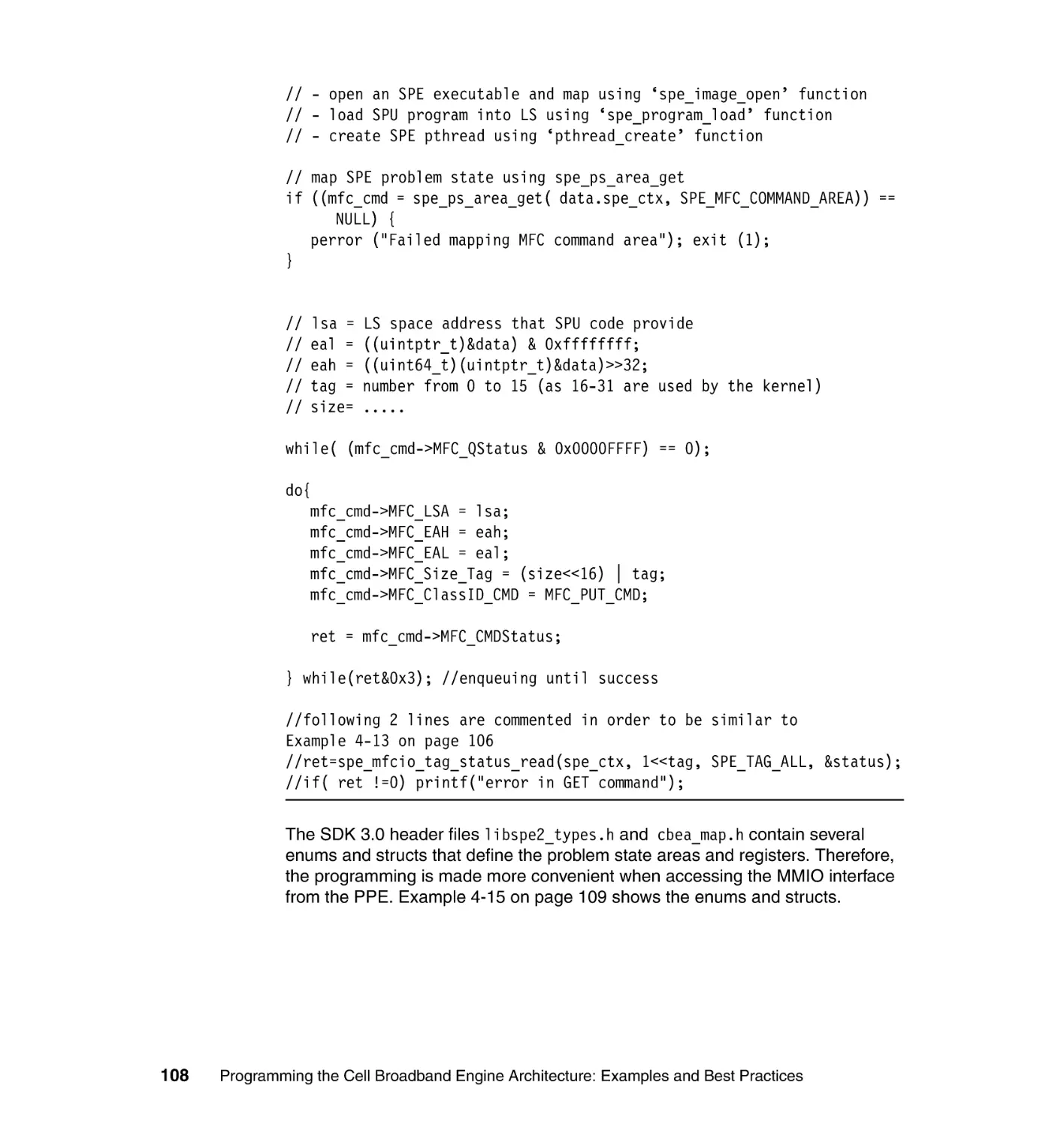
Chapter 4. Cell Broadband Engine programming . . . . . . . . . . . . . . . . . . . 75
4.1 Task parallelism and PPE programming . . . . . . . . . . . . . . . . . . . . . . . . . . 77
4.1.1 PPE architecture and PPU programming . . . . . . . . . . . . . . . . . . . . . 78
4.1.2 Task parallelism and managing SPE threads . . . . . . . . . . . . . . . . . . 83
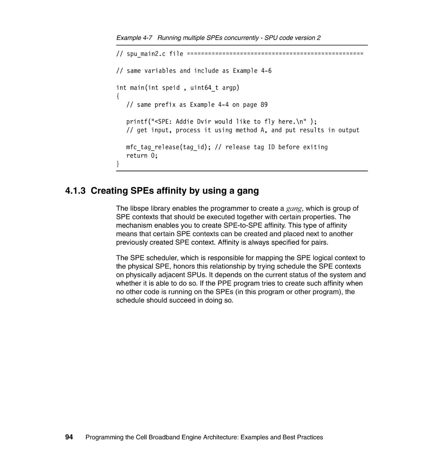
4.1.3 Creating SPEs affinity by using a gang . . . . . . . . . . . . . . . . . . . . . . . 94
4.2 Storage domains, channels, and MMIO interfaces . . . . . . . . . . . . . . . . . . 97
4.2.1 Storage domains . . . . . . . . . . . . . . . . . . . . . . . . . . . . . . . . . . . . . . . . 97
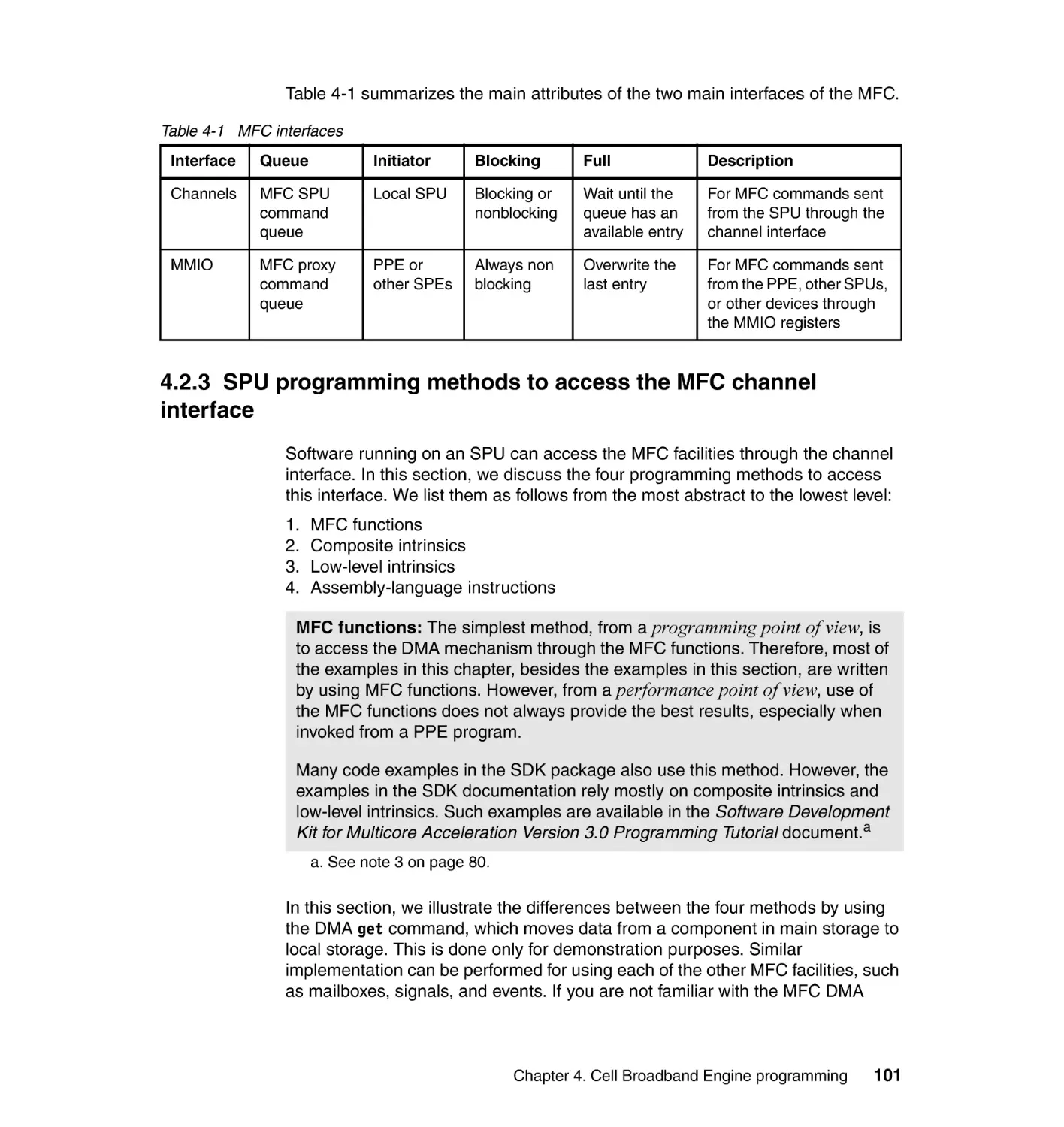
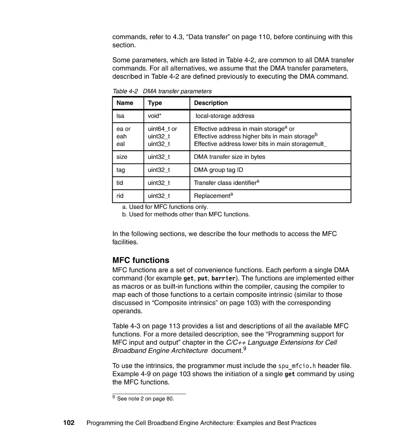
4.2.2 MFC channels and MMIO interfaces and queues . . . . . . . . . . . . . . . 99
4.2.3 SPU programming methods to access the MFC channel interface 101
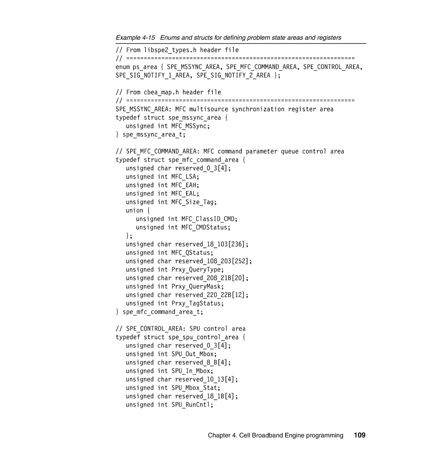
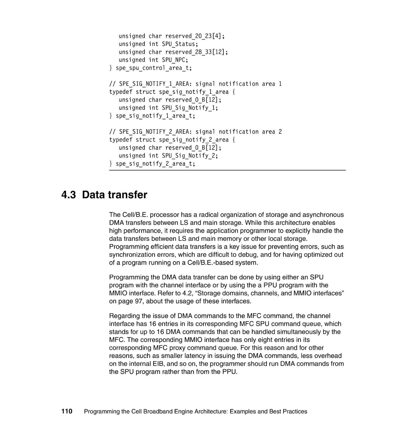
4.2.4 PPU programming methods to access the MFC MMIO interface . . 105
4.3 Data transfer . . . . . . . . . . . . . . . . . . . . . . . . . . . . . . . . . . . . . . . . . . . . . . 110
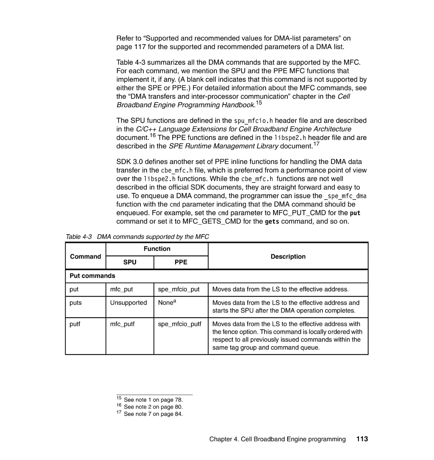
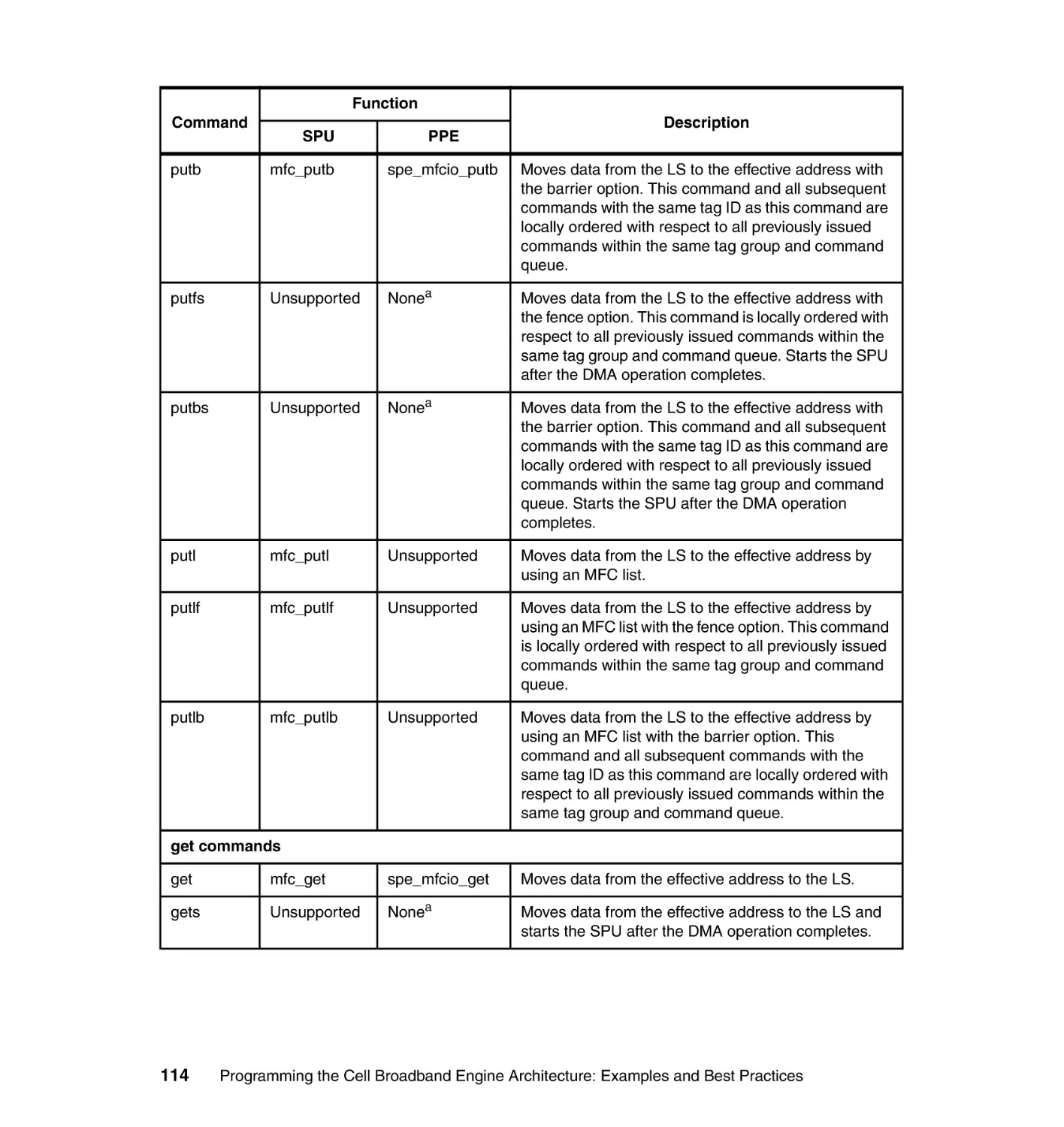
4.3.1 DMA commands . . . . . . . . . . . . . . . . . . . . . . . . . . . . . . . . . . . . . . . 112
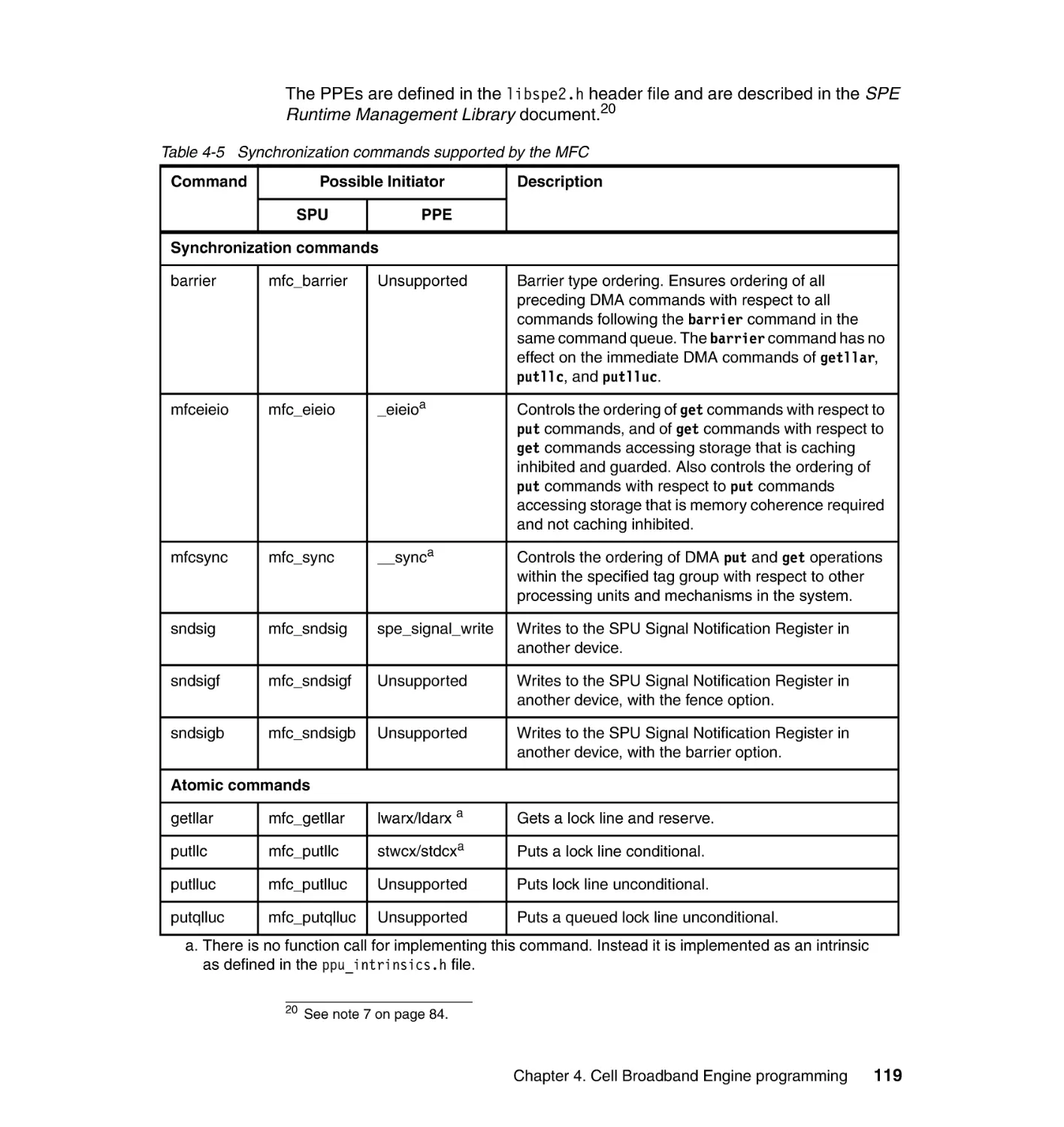
4.3.2 SPE-initiated DMA transfer between the LS and main storage . . . 120
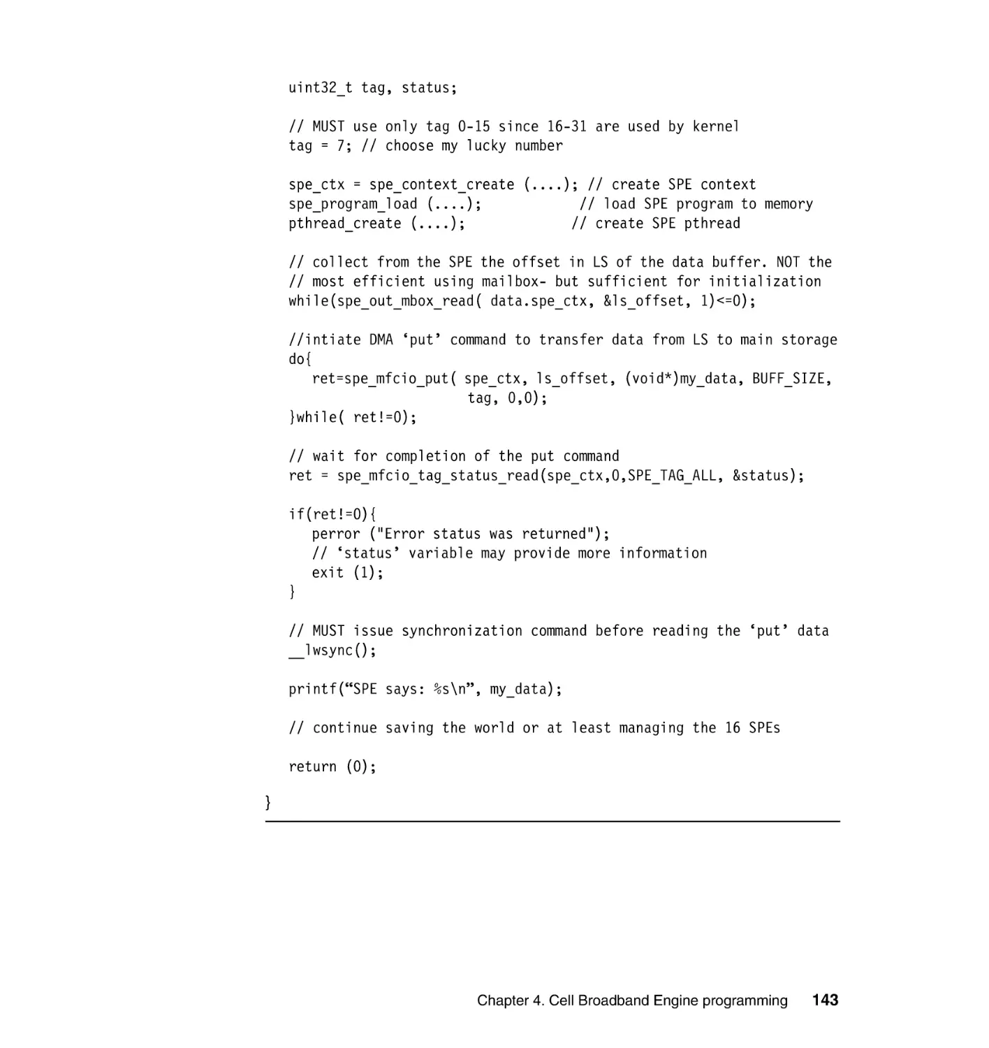
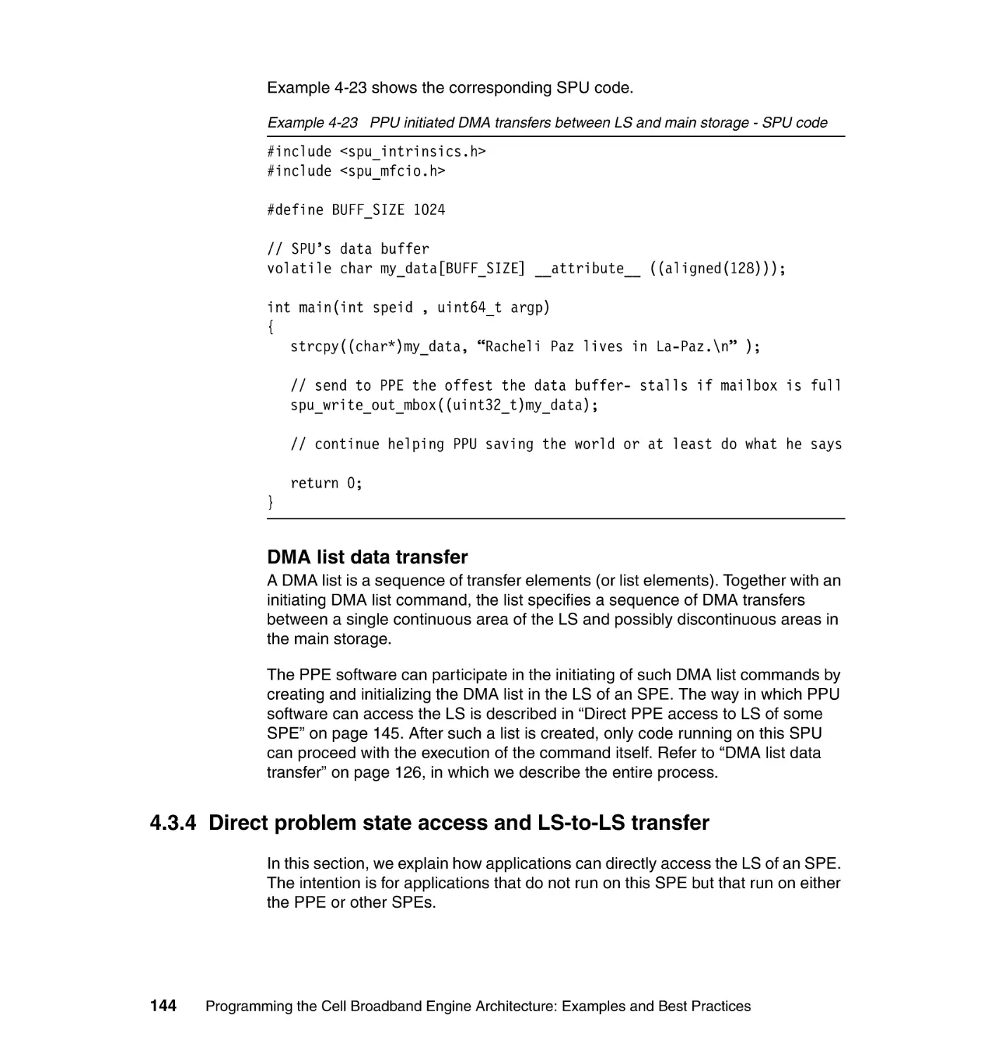
4.3.3 PPU initiated DMA transfer between LS and main storage . . . . . . 138
4.3.4 Direct problem state access and LS-to-LS transfer . . . . . . . . . . . . 144
4.3.5 Facilitating random data access by using the SPU software cache 148
4.3.6 Automatic software caching on SPE . . . . . . . . . . . . . . . . . . . . . . . . 157
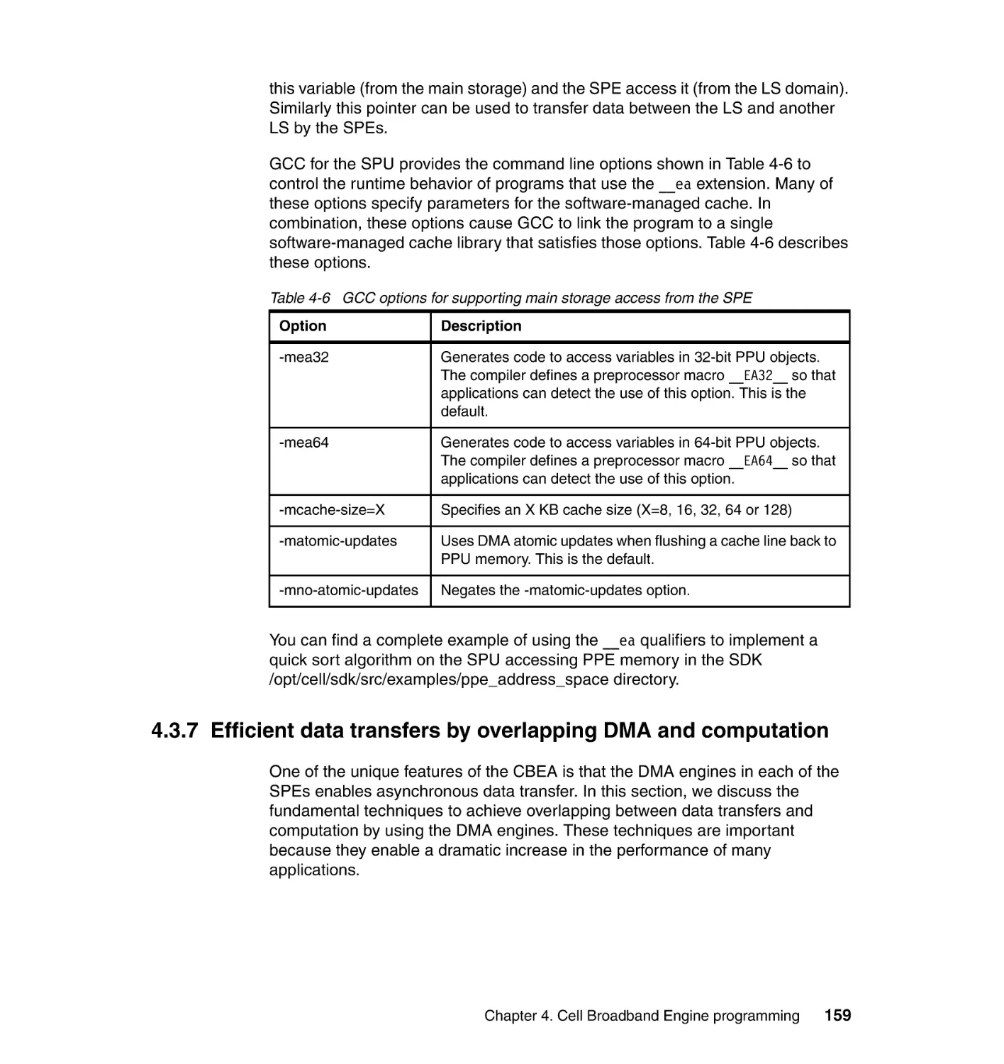
4.3.7 Efficient data transfers by overlapping DMA and computation . . . . 159
4.3.8 Improving the page hit ratio by using huge pages . . . . . . . . . . . . . 166
4.3.9 Improving memory access using NUMA . . . . . . . . . . . . . . . . . . . . . 171
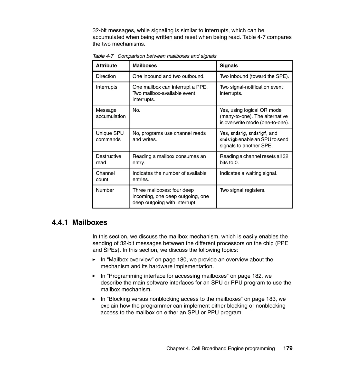
4.4 Inter-processor communication . . . . . . . . . . . . . . . . . . . . . . . . . . . . . . . . 178
4.4.1 Mailboxes . . . . . . . . . . . . . . . . . . . . . . . . . . . . . . . . . . . . . . . . . . . . 179
4.4.2 Signal notification . . . . . . . . . . . . . . . . . . . . . . . . . . . . . . . . . . . . . . 190
4.4.3 SPE events . . . . . . . . . . . . . . . . . . . . . . . . . . . . . . . . . . . . . . . . . . . 203
4.4.4 Atomic unit and atomic cache . . . . . . . . . . . . . . . . . . . . . . . . . . . . . 211
4.5 Shared storage synchronizing and data ordering . . . . . . . . . . . . . . . . . . 218
4.5.1 Shared storage model. . . . . . . . . . . . . . . . . . . . . . . . . . . . . . . . . . . 221
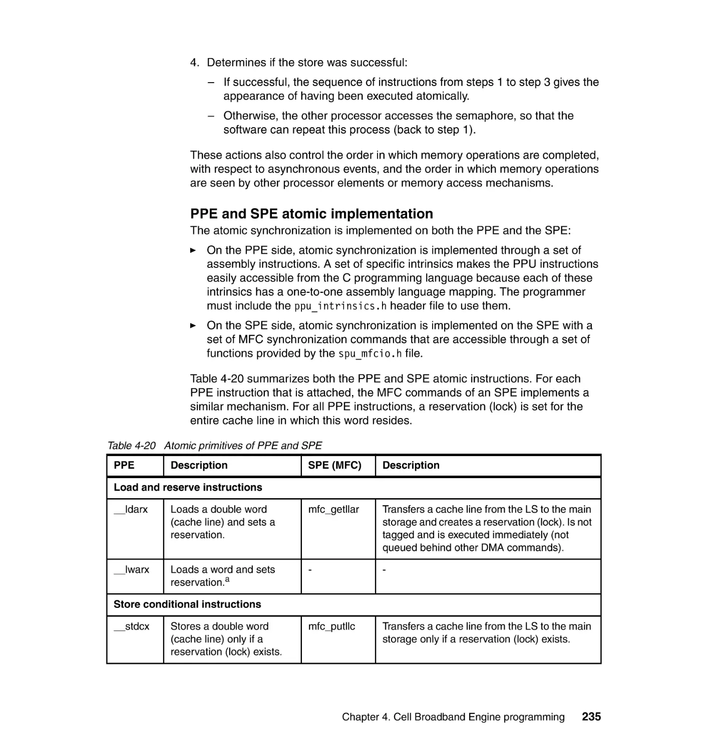
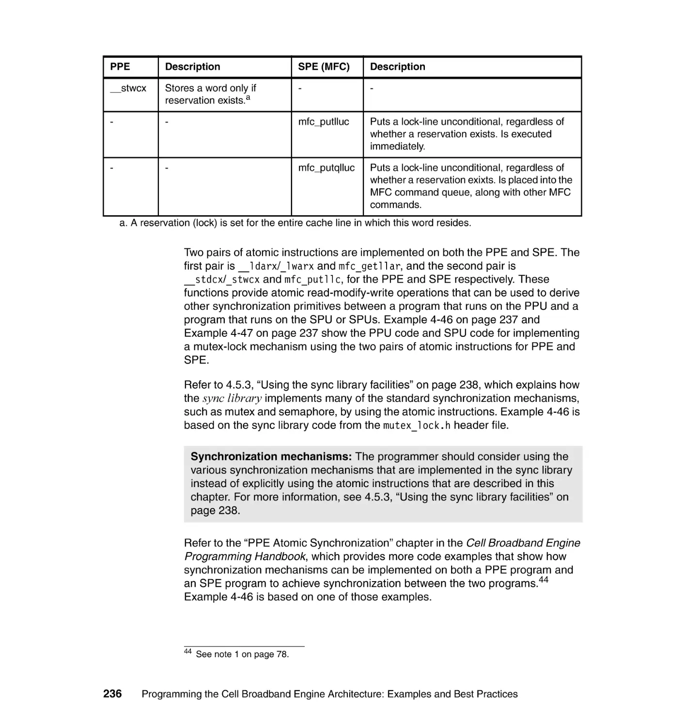
4.5.2 Atomic synchronization . . . . . . . . . . . . . . . . . . . . . . . . . . . . . . . . . . 233
4.5.3 Using the sync library facilities . . . . . . . . . . . . . . . . . . . . . . . . . . . . 238
4.5.4 Practical examples of using ordering and synchronization
mechanisms . . . . . . . . . . . . . . . . . . . . . . . . . . . . . . . . . . . . . . . . . . 240
4.6 SPU programming . . . . . . . . . . . . . . . . . . . . . . . . . . . . . . . . . . . . . . . . . . 244
4.6.1 Architecture overview and its impact on programming . . . . . . . . . . 245
4.6.2 SPU instruction set and C/C++ language extensions (intrinsics) . . 249
4.6.3 Compiler directives . . . . . . . . . . . . . . . . . . . . . . . . . . . . . . . . . . . . . 256
Contents
v
4.6.4 SIMD programming . . . . . . . . . . . . . . . . . . . . . . . . . . . . . . . . . . . . . 258
4.6.5 Auto-SIMDizing by compiler . . . . . . . . . . . . . . . . . . . . . . . . . . . . . . 270
4.6.6 Working with scalars and converting between different vector types277
4.6.7 Code transfer using SPU code overlay . . . . . . . . . . . . . . . . . . . . . . 283
4.6.8 Eliminating and predicting branches . . . . . . . . . . . . . . . . . . . . . . . . 284
4.7 Frameworks and domain-specific libraries . . . . . . . . . . . . . . . . . . . . . . . 289
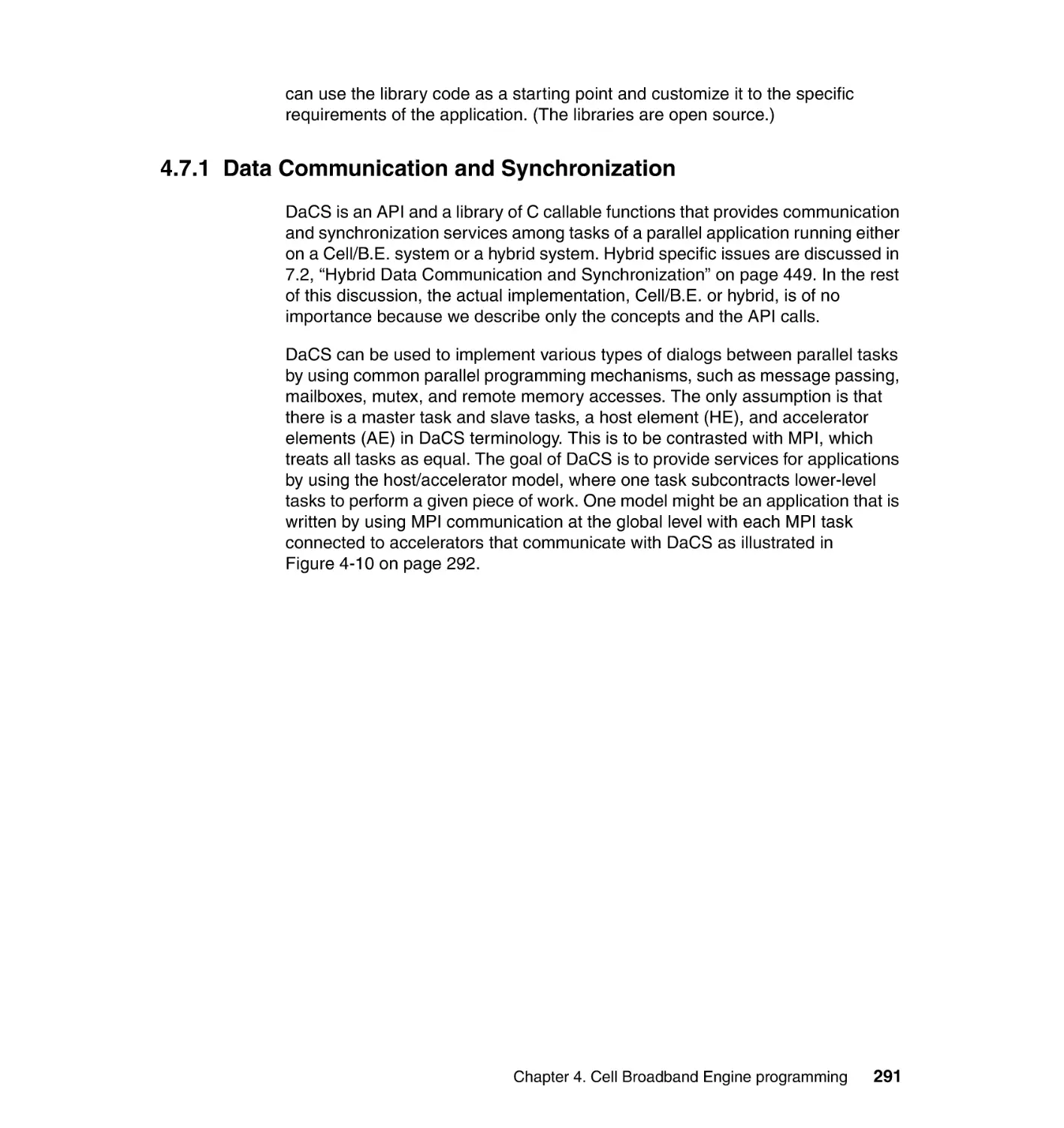
4.7.1 Data Communication and Synchronization . . . . . . . . . . . . . . . . . . . 291
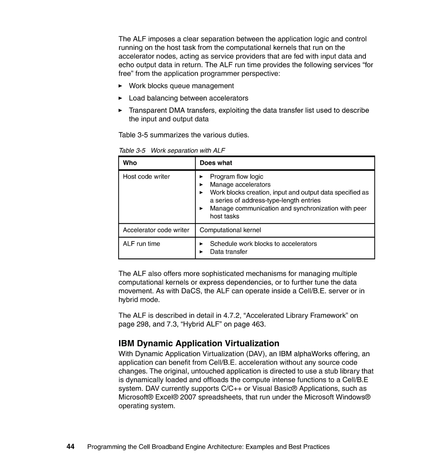
4.7.2 Accelerated Library Framework . . . . . . . . . . . . . . . . . . . . . . . . . . . 298
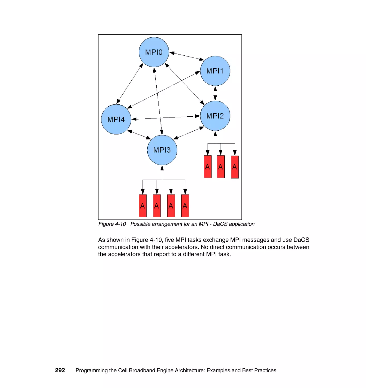
4.7.3 Domain-specific libraries . . . . . . . . . . . . . . . . . . . . . . . . . . . . . . . . . 314
4.8 Programming guidelines . . . . . . . . . . . . . . . . . . . . . . . . . . . . . . . . . . . . . 319
4.8.1 General guidelines . . . . . . . . . . . . . . . . . . . . . . . . . . . . . . . . . . . . . 320
4.8.2 SPE programming guidelines . . . . . . . . . . . . . . . . . . . . . . . . . . . . . 321
4.8.3 Data transfers and synchronization guidelines . . . . . . . . . . . . . . . . 325
4.8.4 Inter-processor communication . . . . . . . . . . . . . . . . . . . . . . . . . . . . 328
Chapter 5. Programming tools and debugging techniques . . . . . . . . . . 329
5.1 Tools taxonomy and basic time line approach . . . . . . . . . . . . . . . . . . . . 330
5.1.1 Dual toolchain . . . . . . . . . . . . . . . . . . . . . . . . . . . . . . . . . . . . . . . . . 330
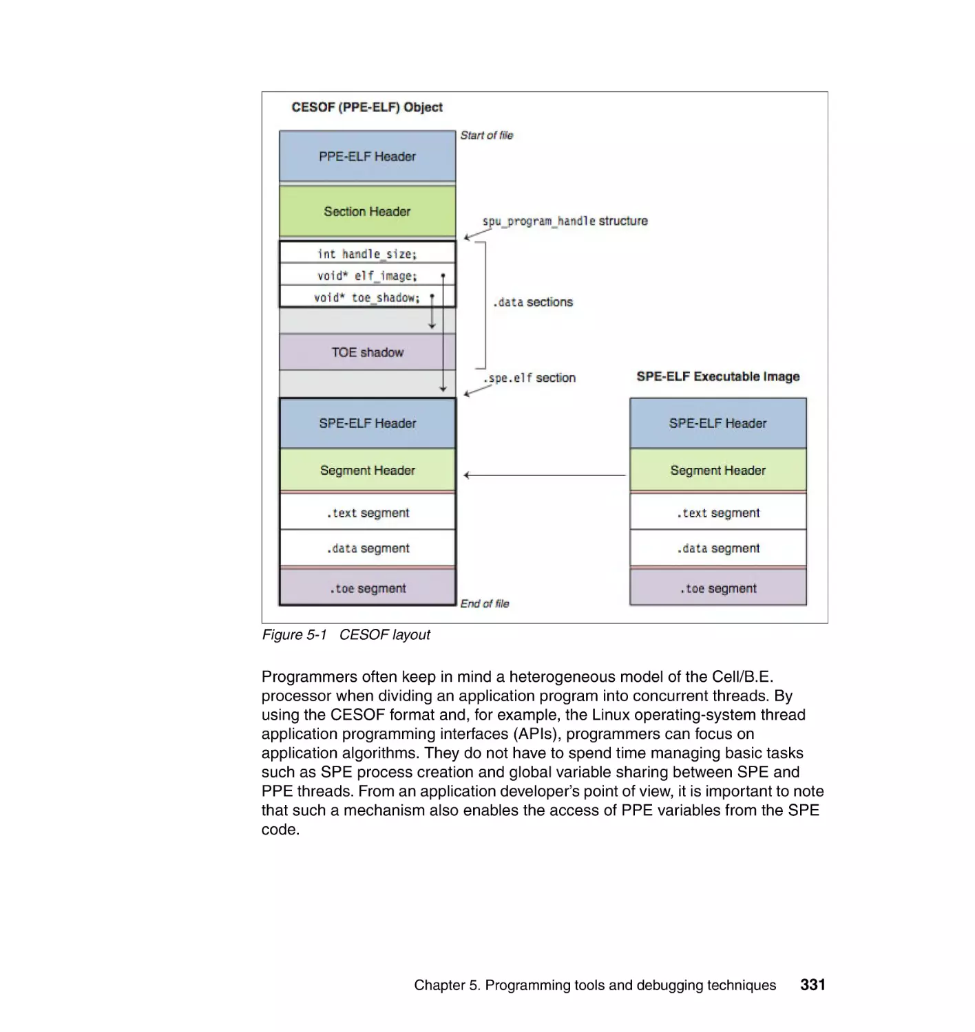
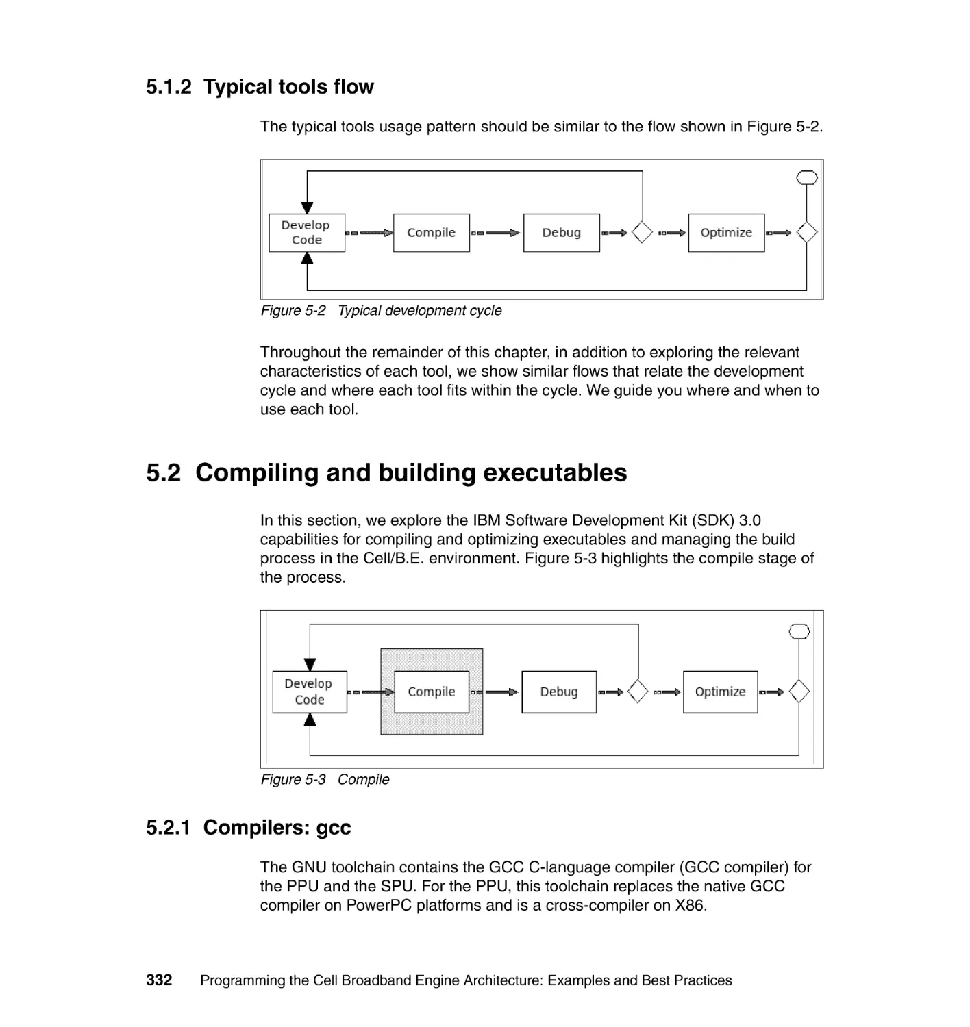
5.1.2 Typical tools flow. . . . . . . . . . . . . . . . . . . . . . . . . . . . . . . . . . . . . . . 332
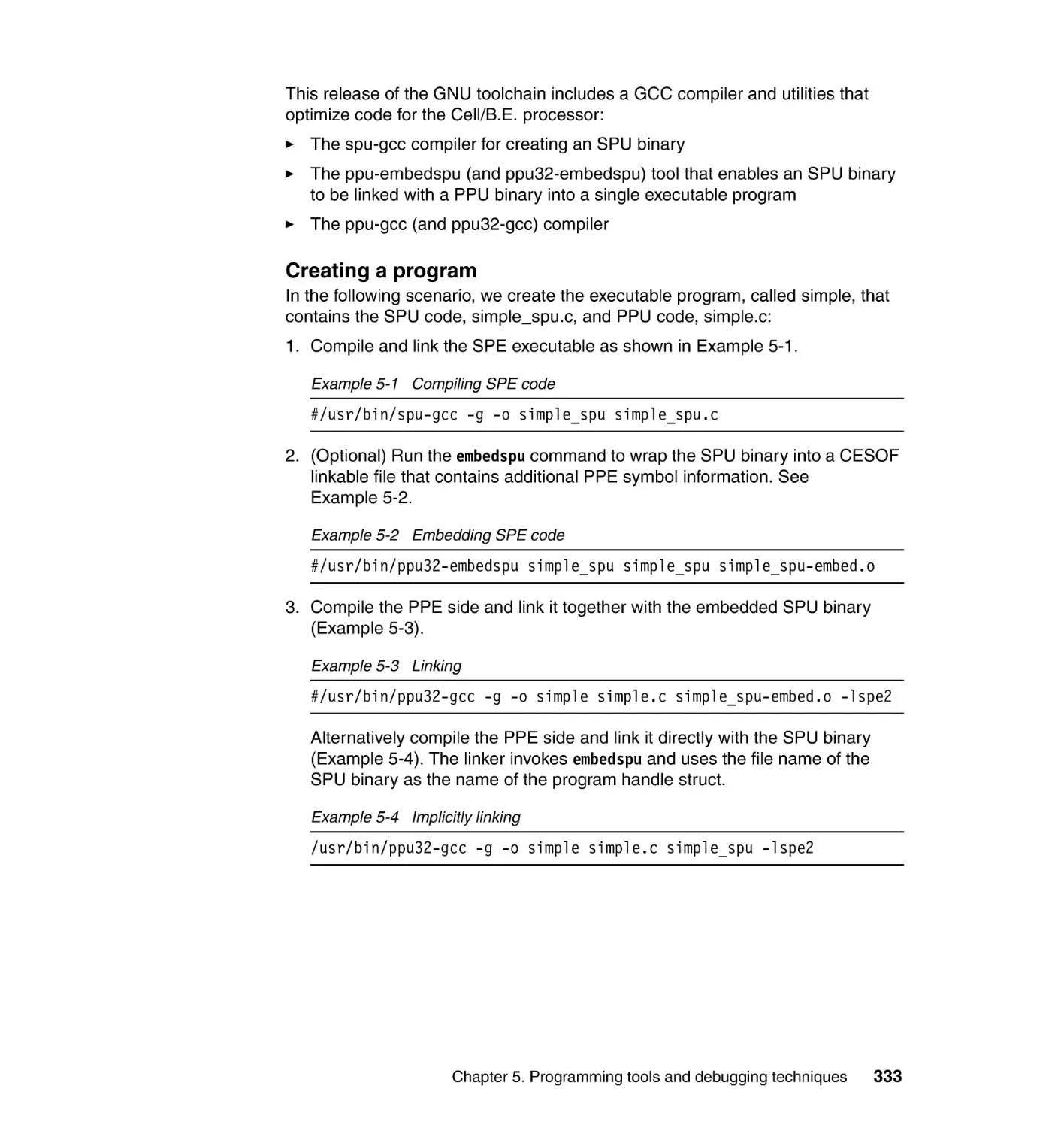
5.2 Compiling and building executables . . . . . . . . . . . . . . . . . . . . . . . . . . . . 332
5.2.1 Compilers: gcc . . . . . . . . . . . . . . . . . . . . . . . . . . . . . . . . . . . . . . . . 332
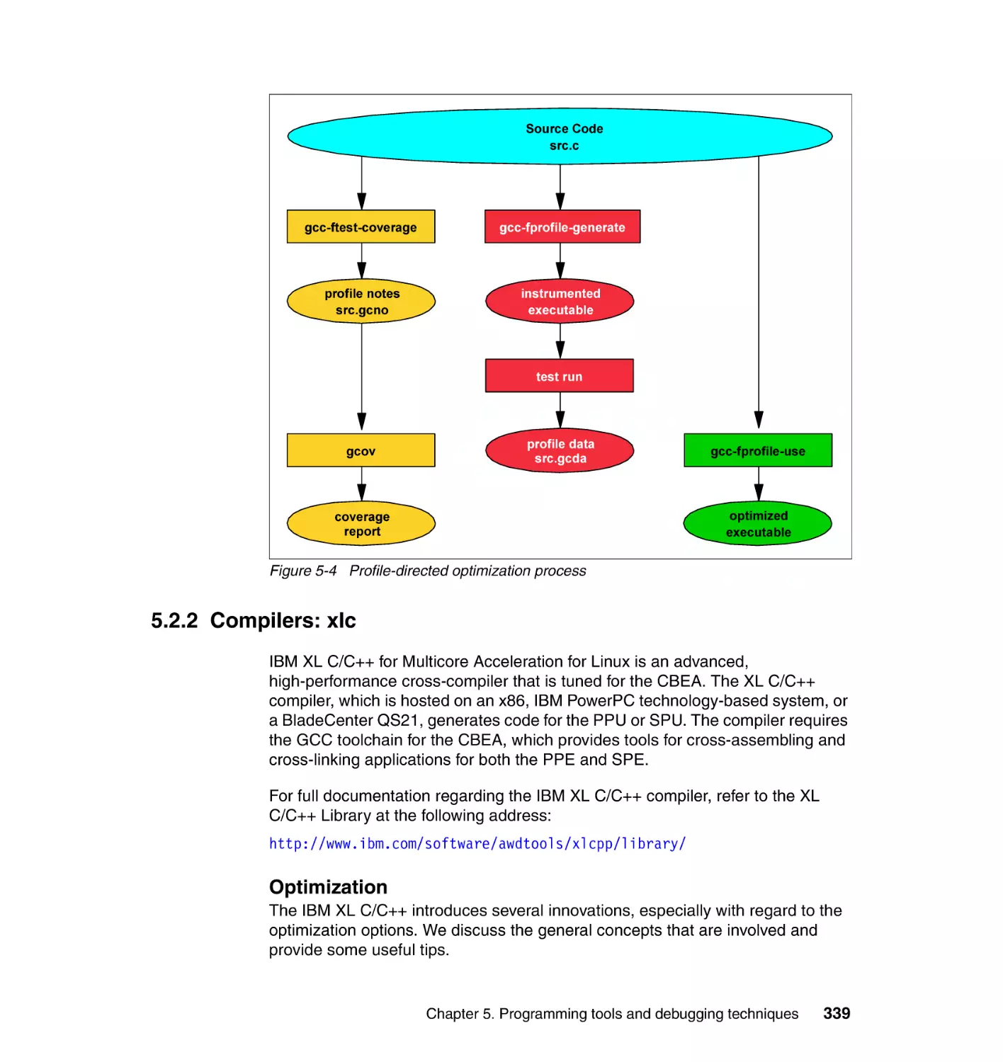
5.2.2 Compilers: xlc . . . . . . . . . . . . . . . . . . . . . . . . . . . . . . . . . . . . . . . . . 339
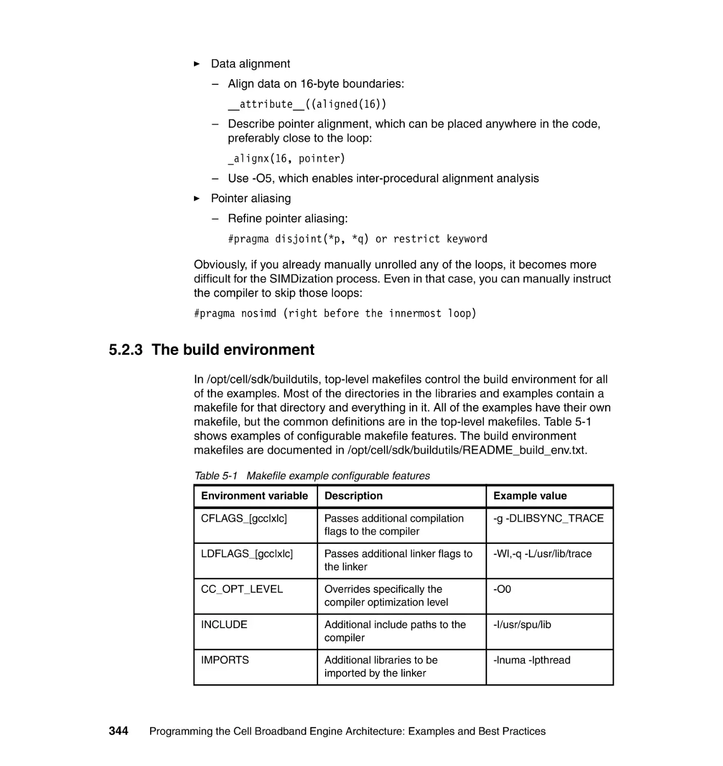
5.2.3 The build environment. . . . . . . . . . . . . . . . . . . . . . . . . . . . . . . . . . . 344
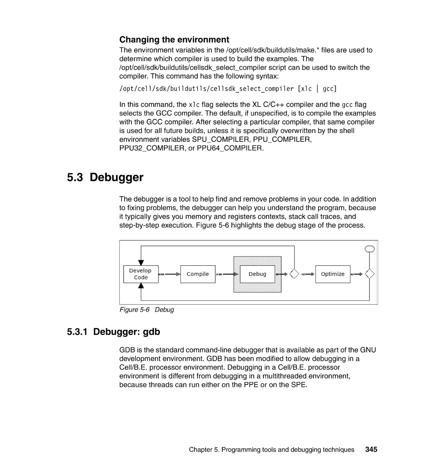
5.3 Debugger. . . . . . . . . . . . . . . . . . . . . . . . . . . . . . . . . . . . . . . . . . . . . . . . . 345
5.3.1 Debugger: gdb . . . . . . . . . . . . . . . . . . . . . . . . . . . . . . . . . . . . . . . . 345
5.4 IBM Full System Simulator . . . . . . . . . . . . . . . . . . . . . . . . . . . . . . . . . . . 354
5.4.1 Setting up and bringing up the simulator. . . . . . . . . . . . . . . . . . . . . 356
5.4.2 Operating the simulator GUI . . . . . . . . . . . . . . . . . . . . . . . . . . . . . . 357
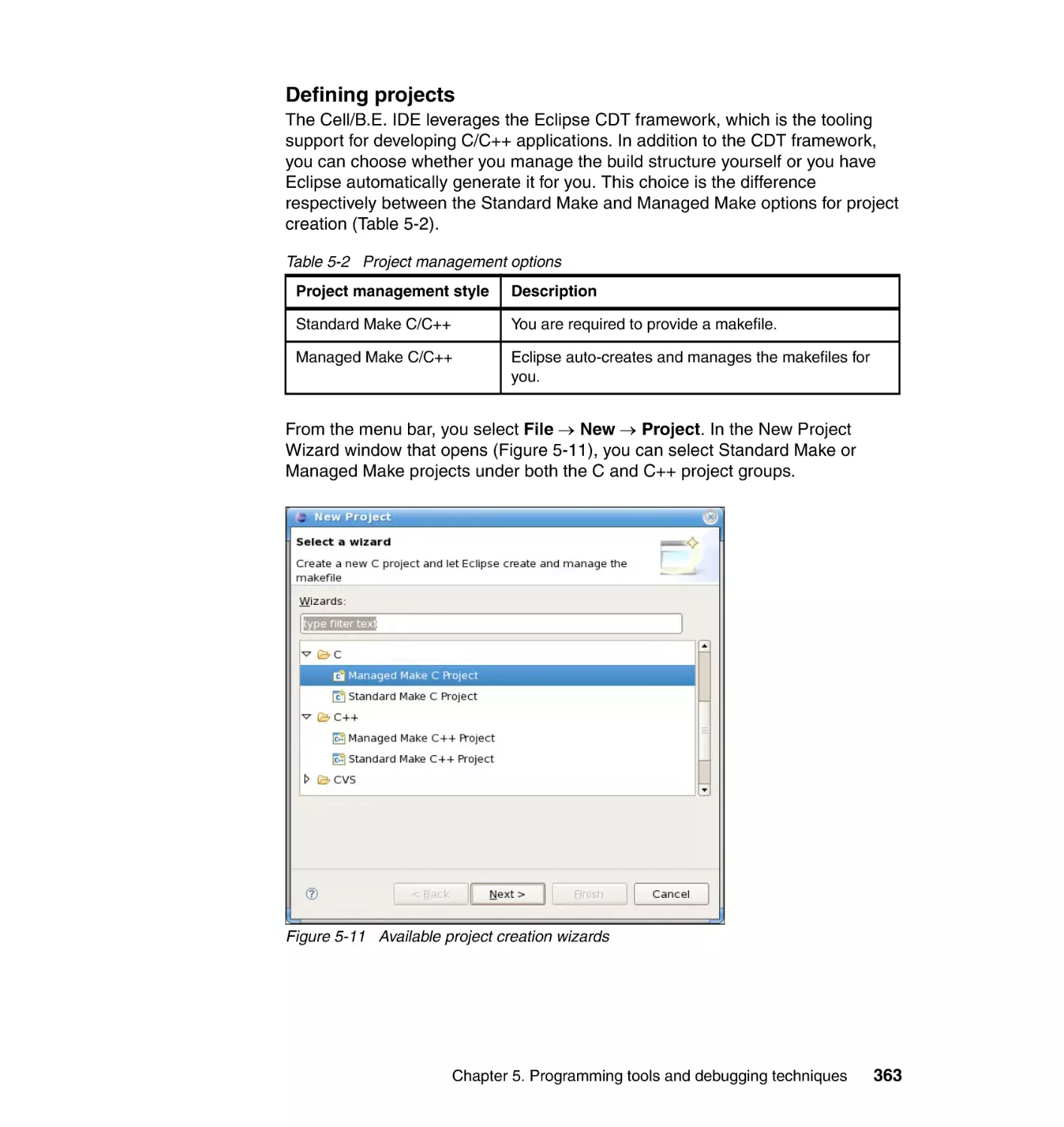
5.5 IBM Multicore Acceleration Integrated Development Environment . . . . . 362
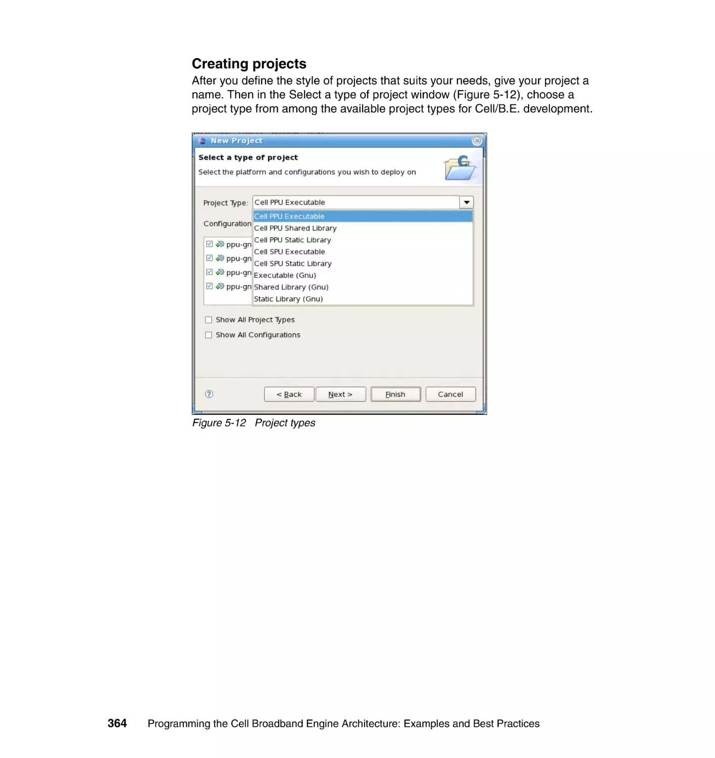
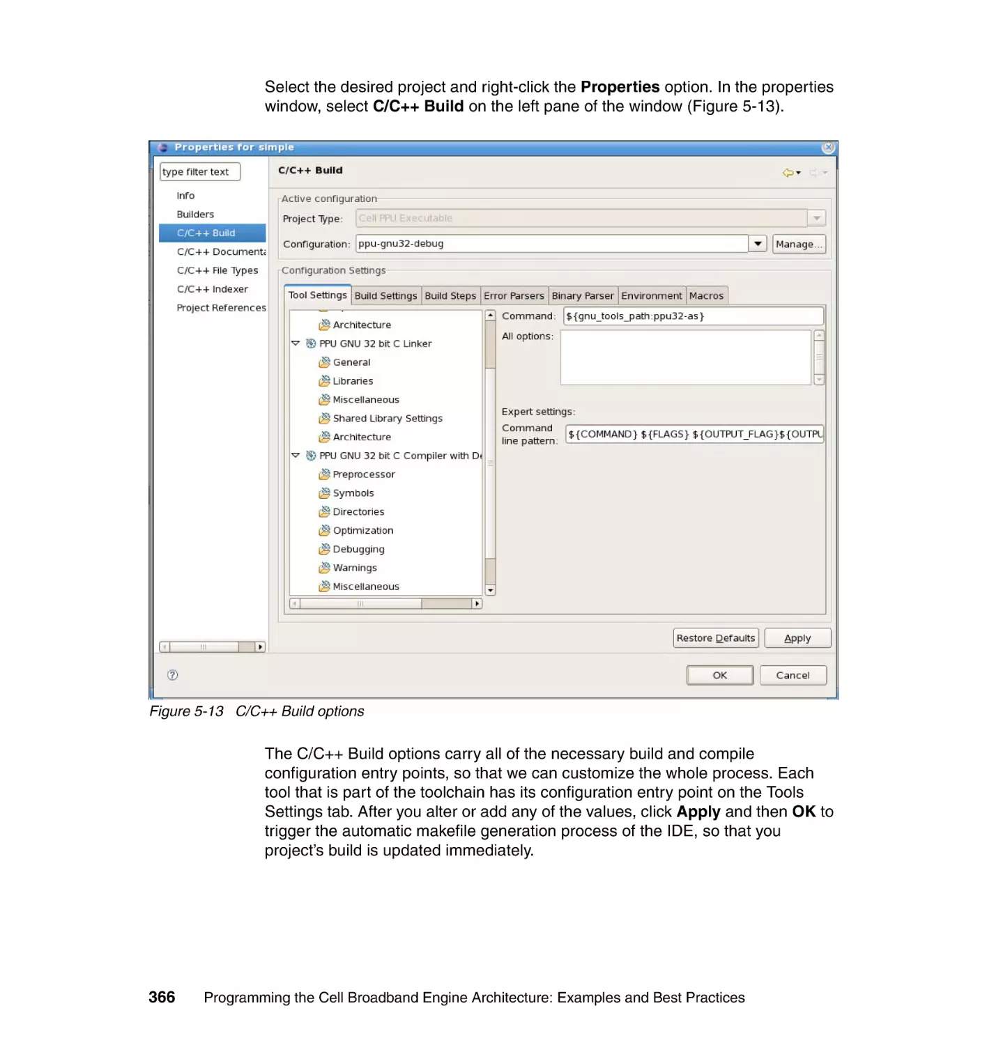
5.5.1 Step 1: Setting up a project. . . . . . . . . . . . . . . . . . . . . . . . . . . . . . . 362
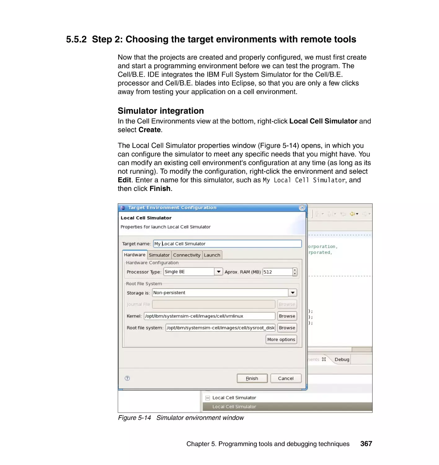
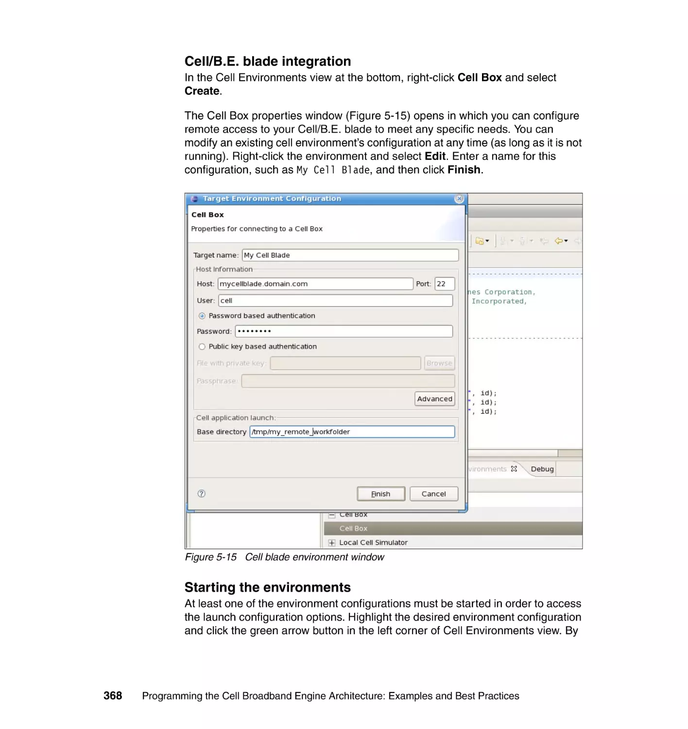
5.5.2 Step 2: Choosing the target environments with remote tools . . . . . 367
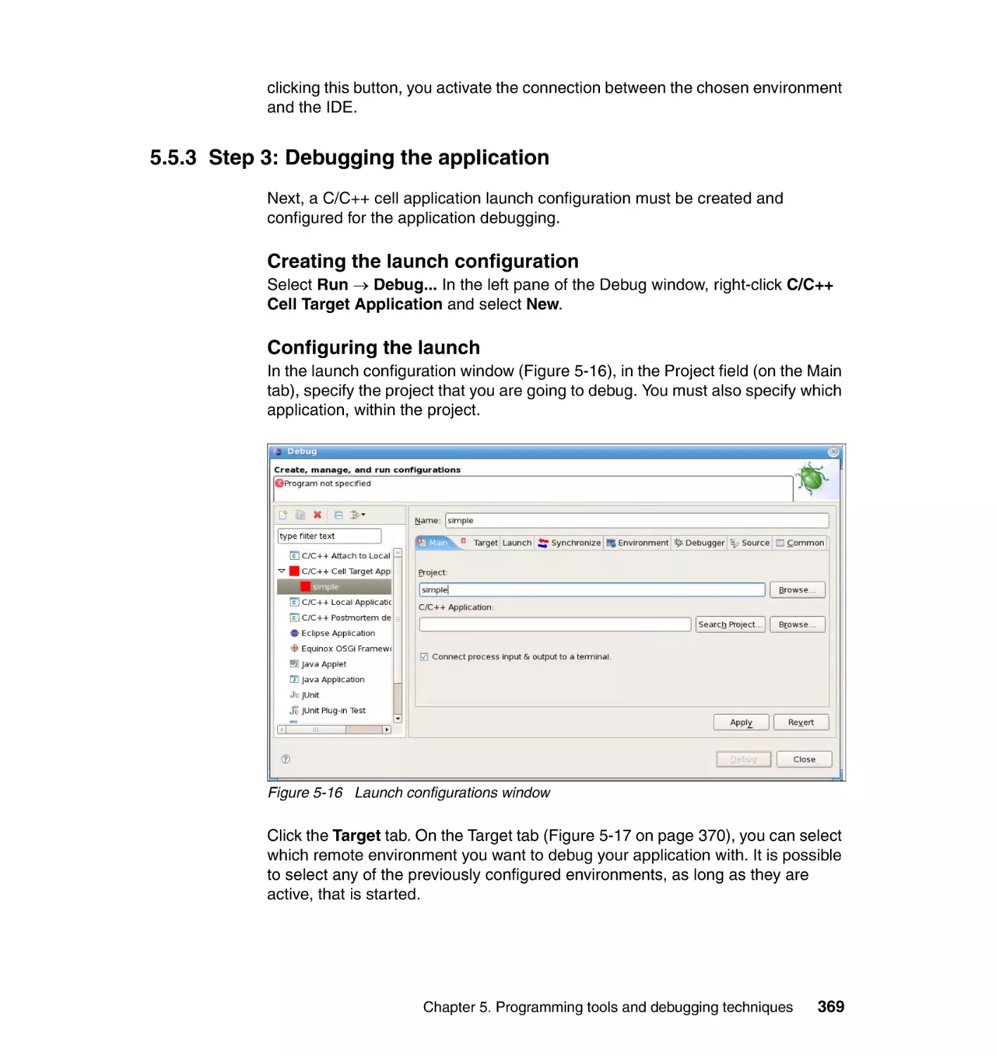
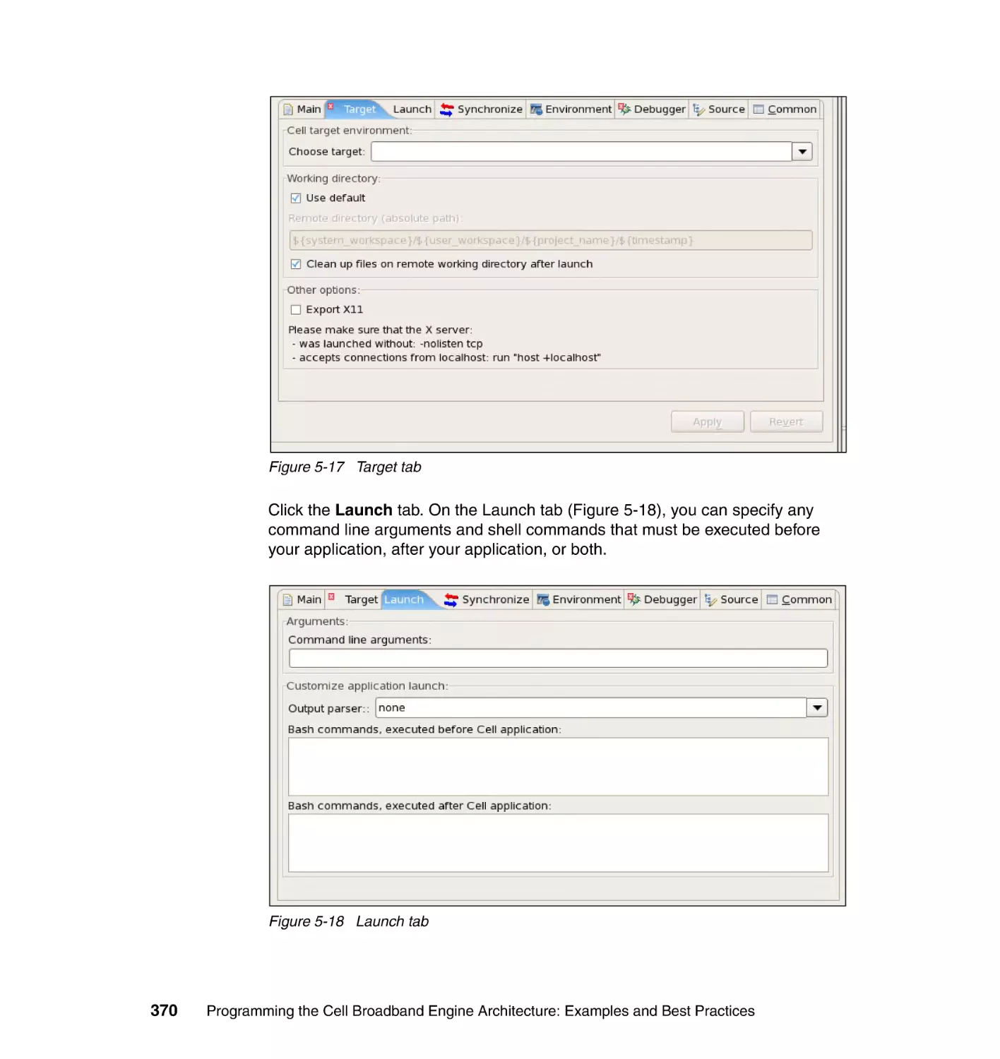
5.5.3 Step 3: Debugging the application . . . . . . . . . . . . . . . . . . . . . . . . . 369
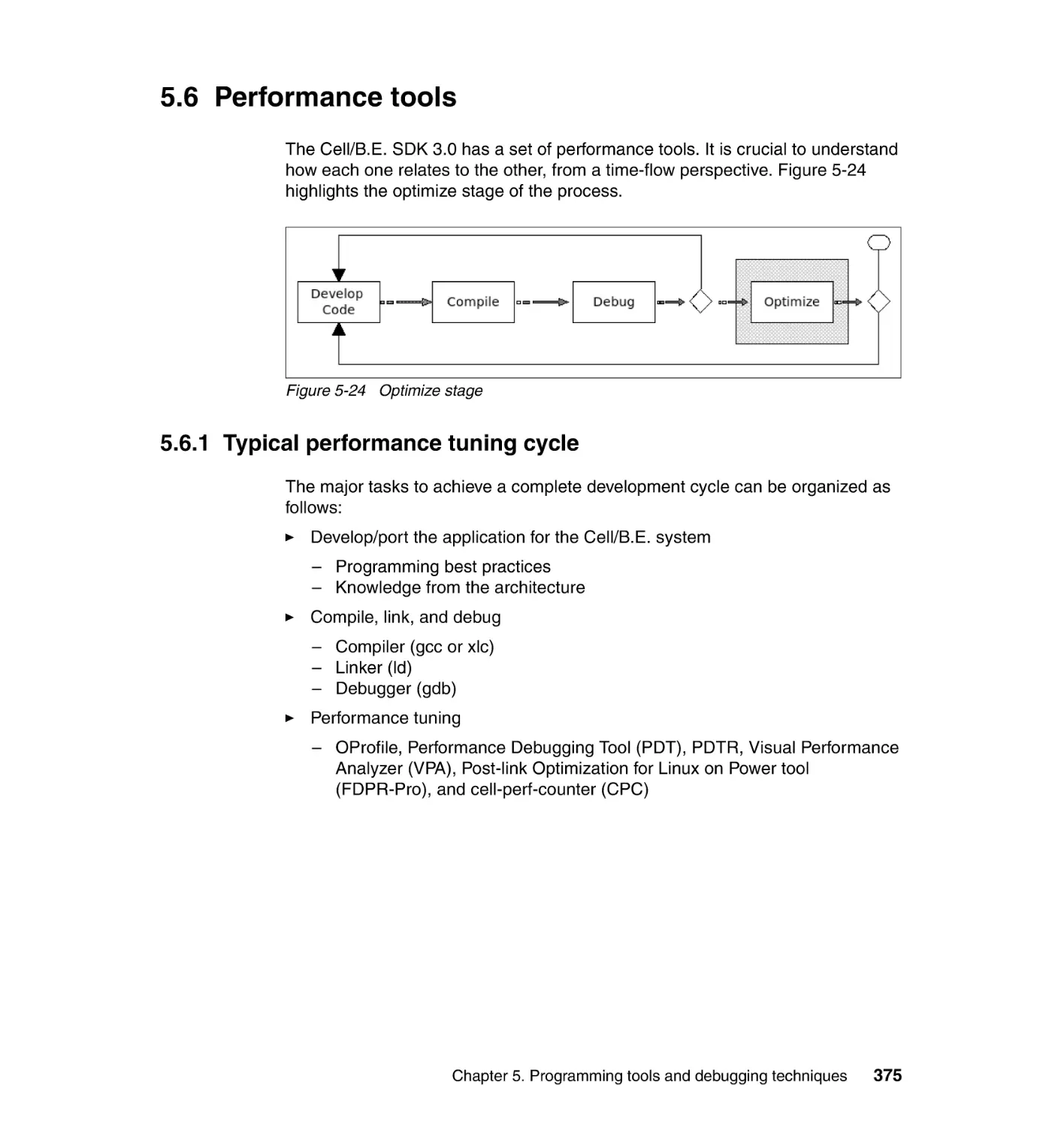
5.6 Performance tools . . . . . . . . . . . . . . . . . . . . . . . . . . . . . . . . . . . . . . . . . . 375
5.6.1 Typical performance tuning cycle . . . . . . . . . . . . . . . . . . . . . . . . . . 375
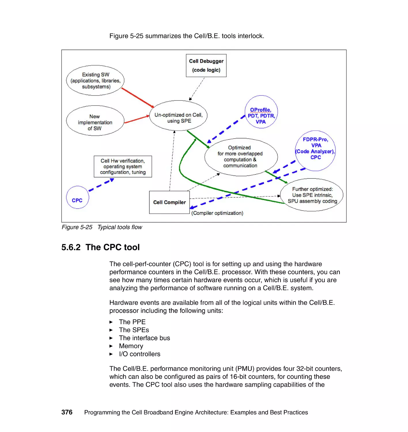
5.6.2 The CPC tool. . . . . . . . . . . . . . . . . . . . . . . . . . . . . . . . . . . . . . . . . . 376
5.6.3 OProfile . . . . . . . . . . . . . . . . . . . . . . . . . . . . . . . . . . . . . . . . . . . . . . 382
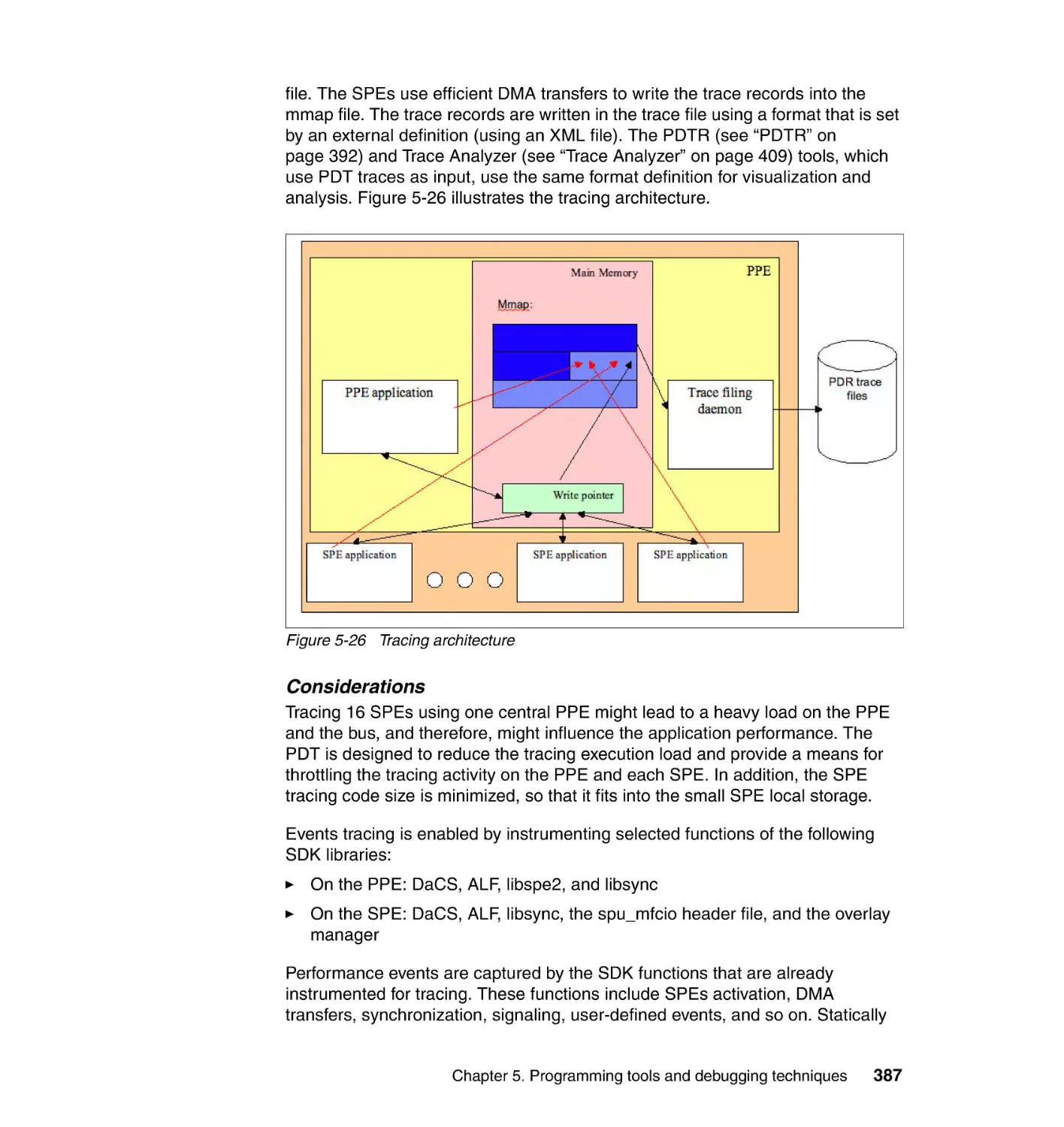
5.6.4 Performance Debugging Tool . . . . . . . . . . . . . . . . . . . . . . . . . . . . . 386
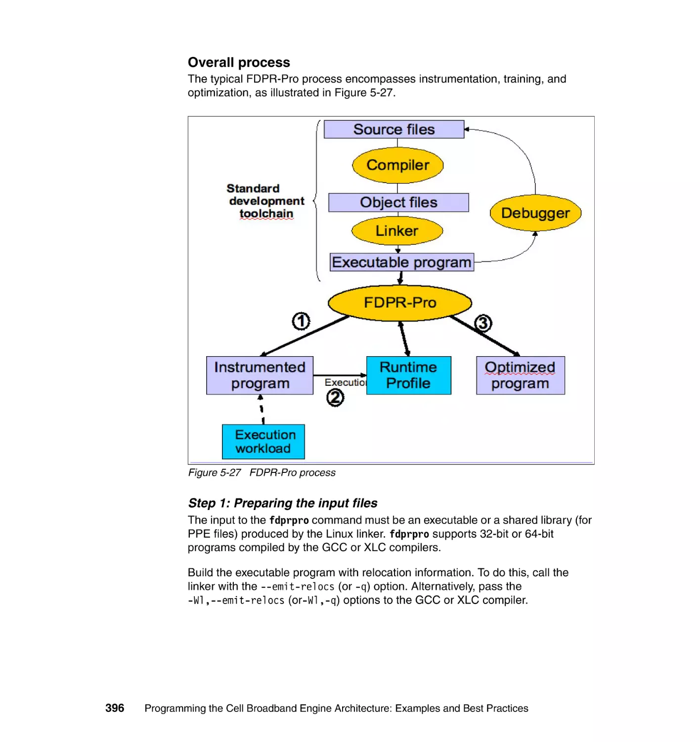
5.6.5 FDPR-Pro . . . . . . . . . . . . . . . . . . . . . . . . . . . . . . . . . . . . . . . . . . . . 394
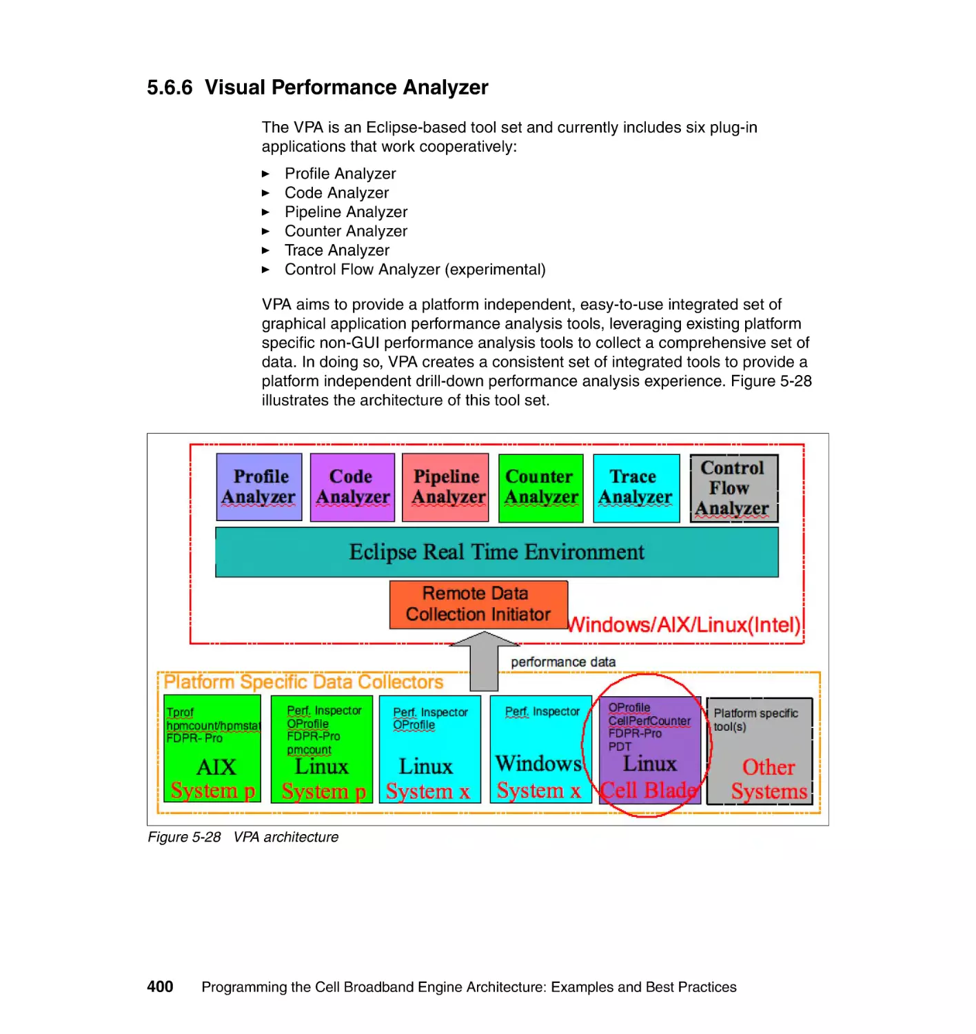
5.6.6 Visual Performance Analyzer . . . . . . . . . . . . . . . . . . . . . . . . . . . . . 400
vi
Programming the Cell Broadband Engine Architecture: Examples and Best Practices
Chapter 6. The performance tools . . . . . . . . . . . . . . . . . . . . . . . . . . . . . . . 417
6.1 Analysis of the FFT16M application . . . . . . . . . . . . . . . . . . . . . . . . . . . . 418
6.2 Preparing and building for profiling . . . . . . . . . . . . . . . . . . . . . . . . . . . . . 418
6.2.1 Step 1: Copying the application from SDK tree. . . . . . . . . . . . . . . . 418
6.2.2 Step 2: Preparing the makefile . . . . . . . . . . . . . . . . . . . . . . . . . . . . 418
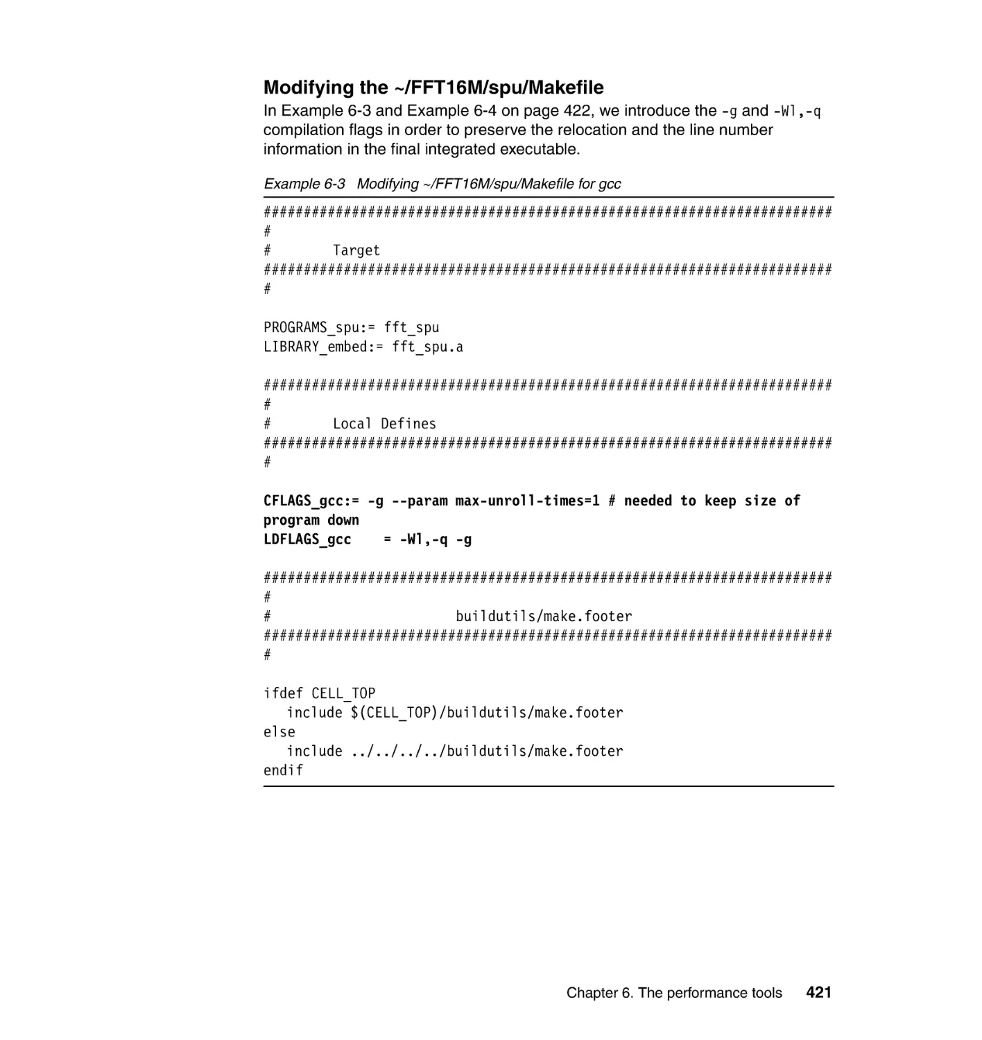
6.3 Creating and working with the profile data . . . . . . . . . . . . . . . . . . . . . . . 423
6.3.1 Step 1: Collecting data with CPC . . . . . . . . . . . . . . . . . . . . . . . . . . 423
6.3.2 Step 2: Visualizing counter information using Counter Analyzer . . 423
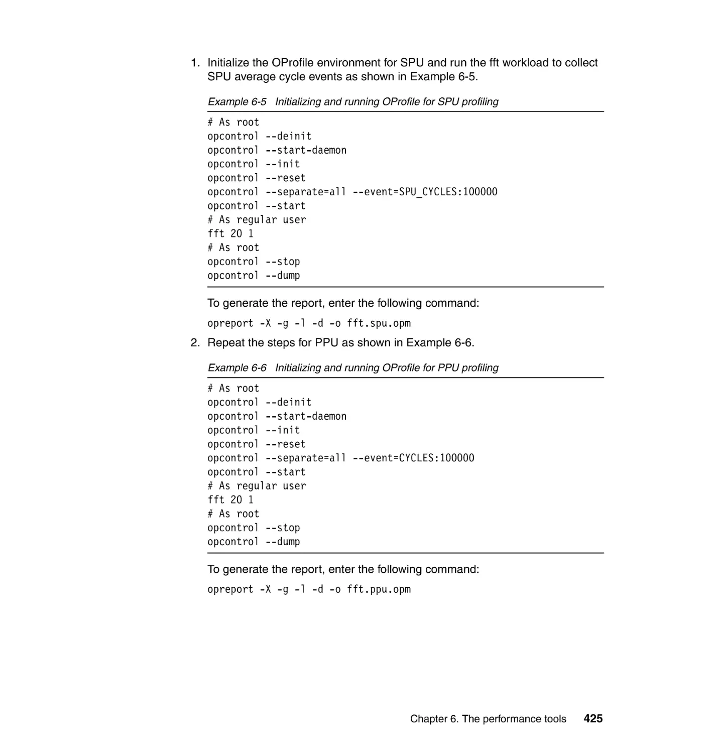
6.3.3 Step 3: Collecting data with OProfile. . . . . . . . . . . . . . . . . . . . . . . . 424
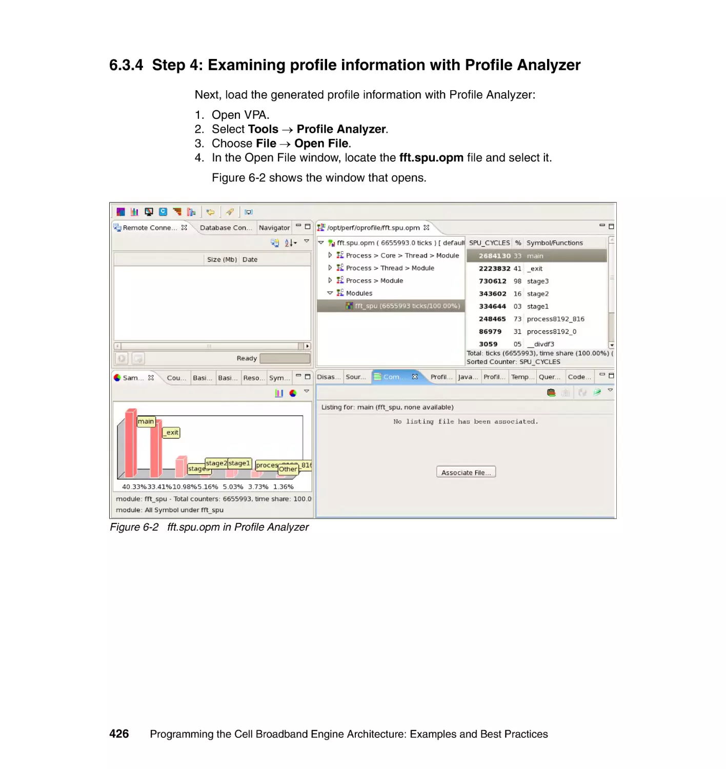
6.3.4 Step 4: Examining profile information with Profile Analyzer . . . . . . 426
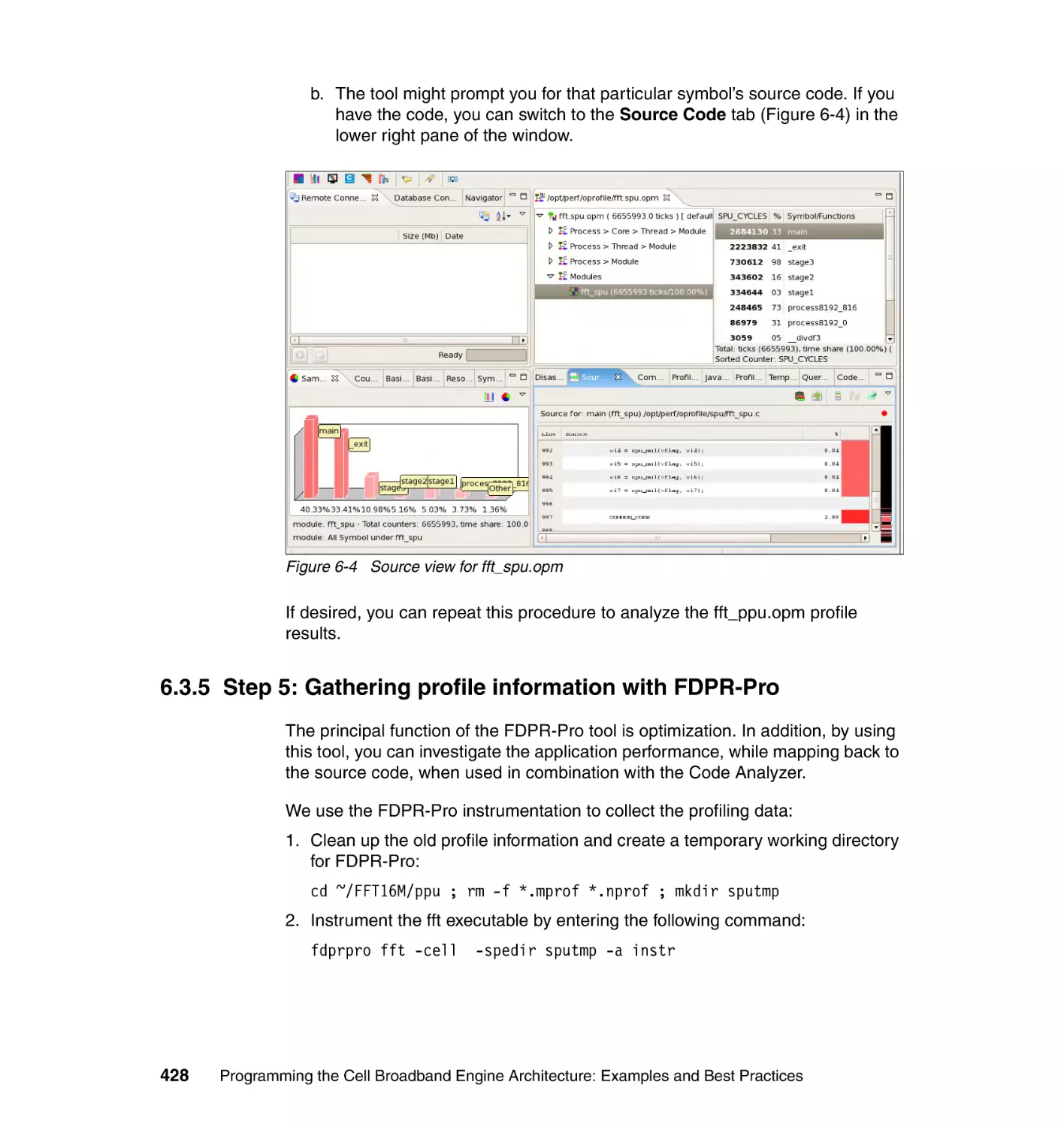
6.3.5 Step 5: Gathering profile information with FDPR-Pro . . . . . . . . . . . 428
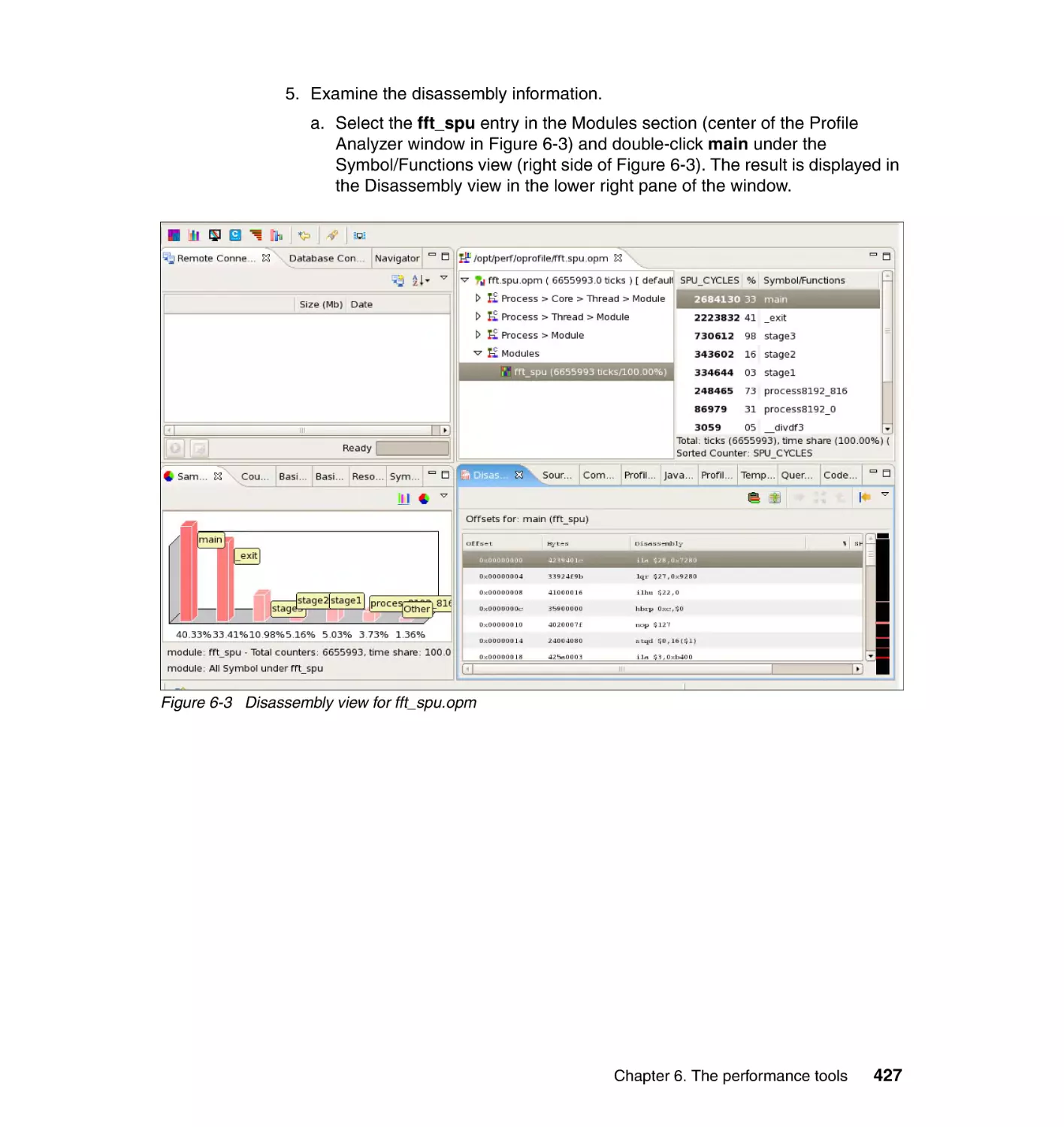
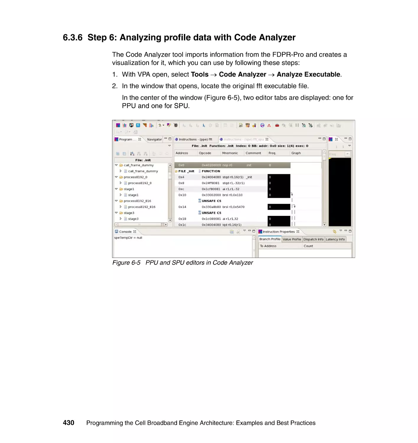
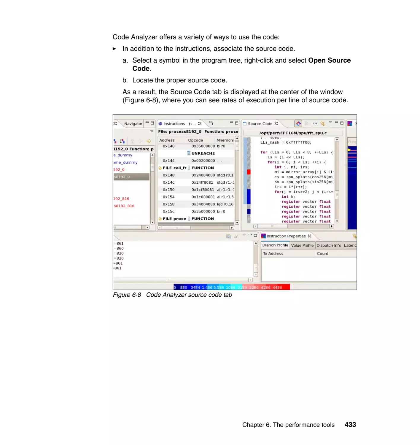
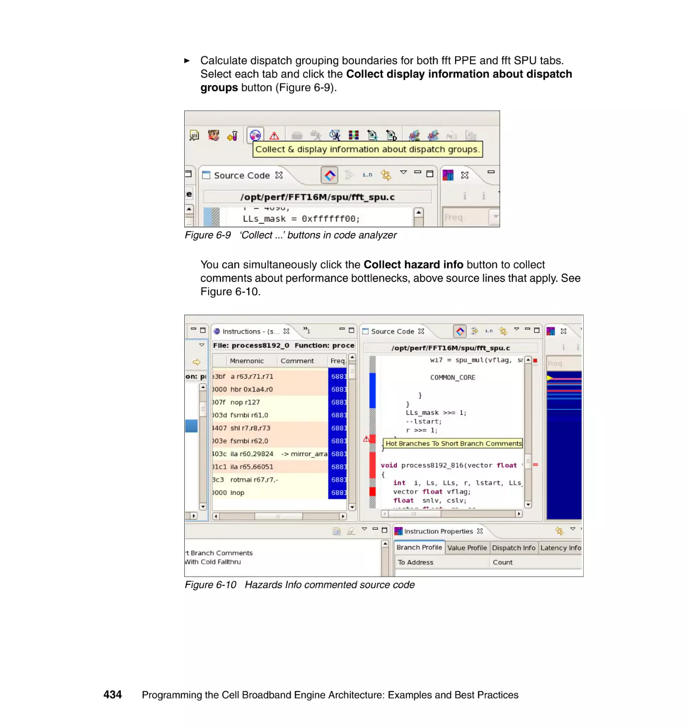
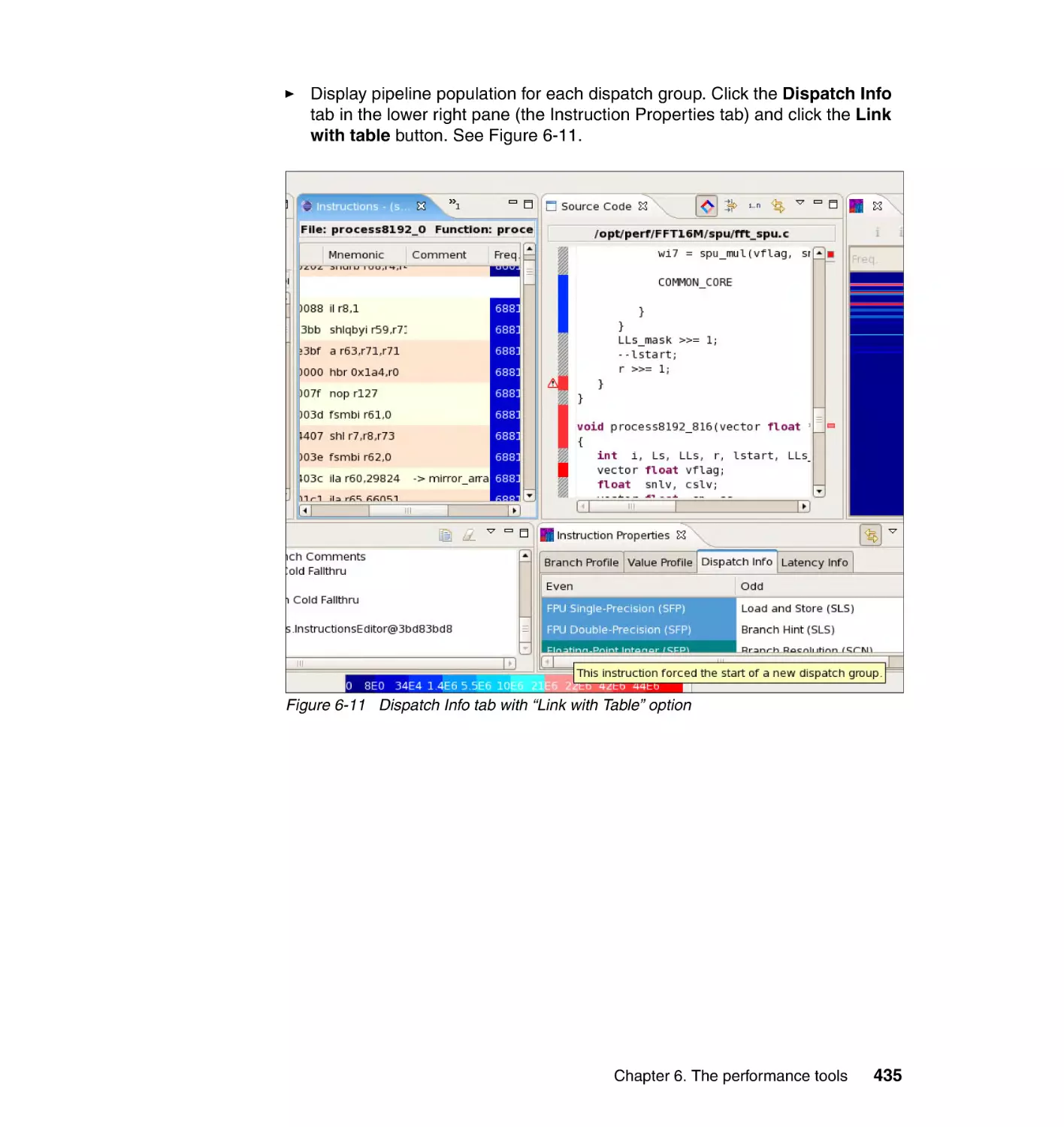
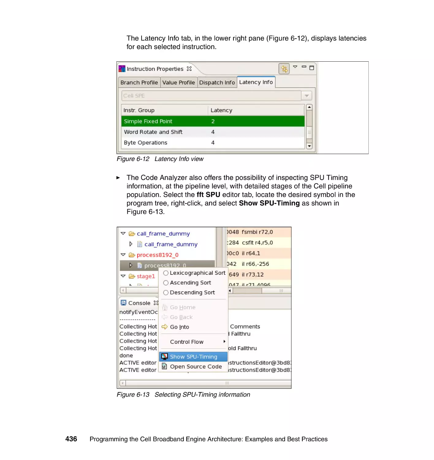
6.3.6 Step 6: Analyzing profile data with Code Analyzer . . . . . . . . . . . . . 430
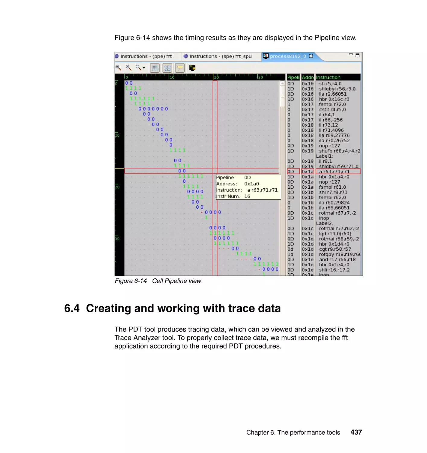
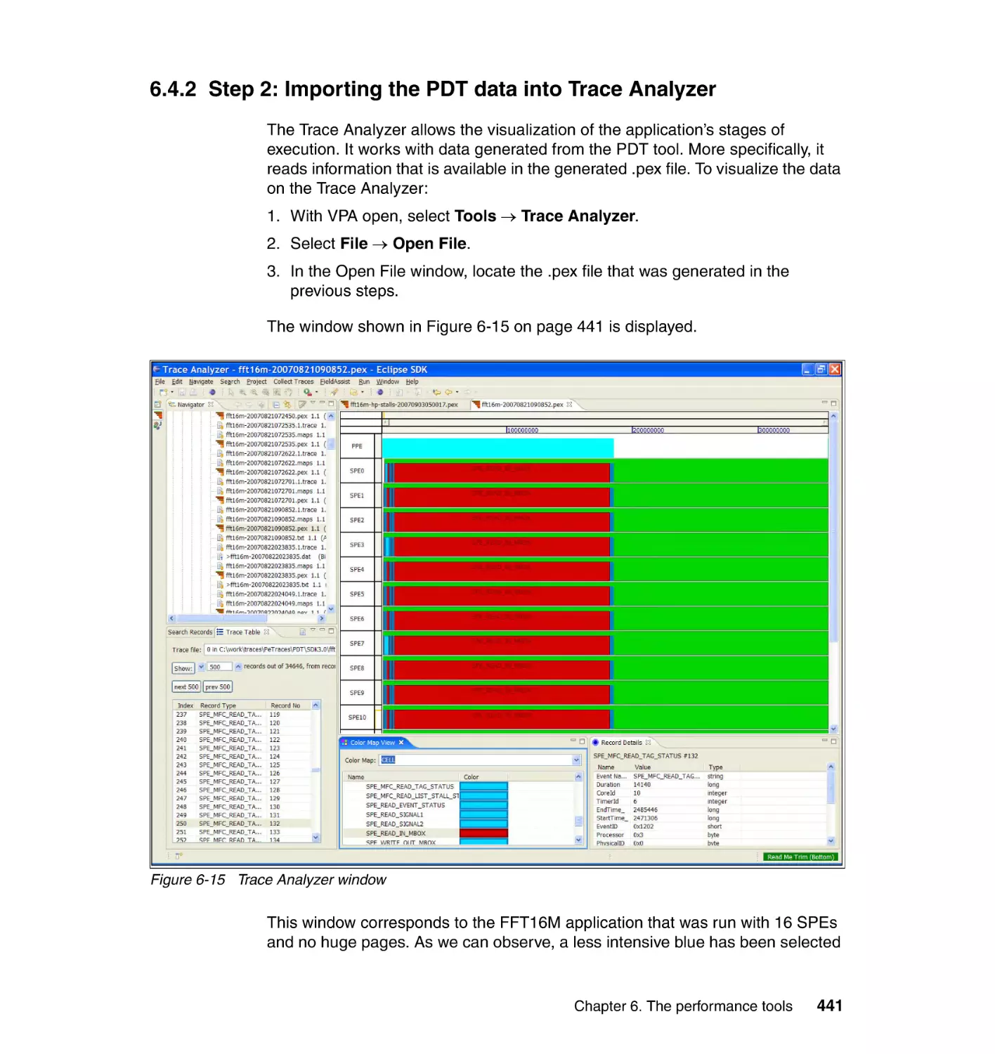
6.4 Creating and working with trace data . . . . . . . . . . . . . . . . . . . . . . . . . . . 437
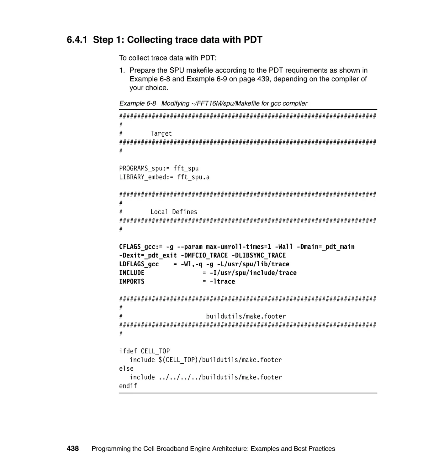
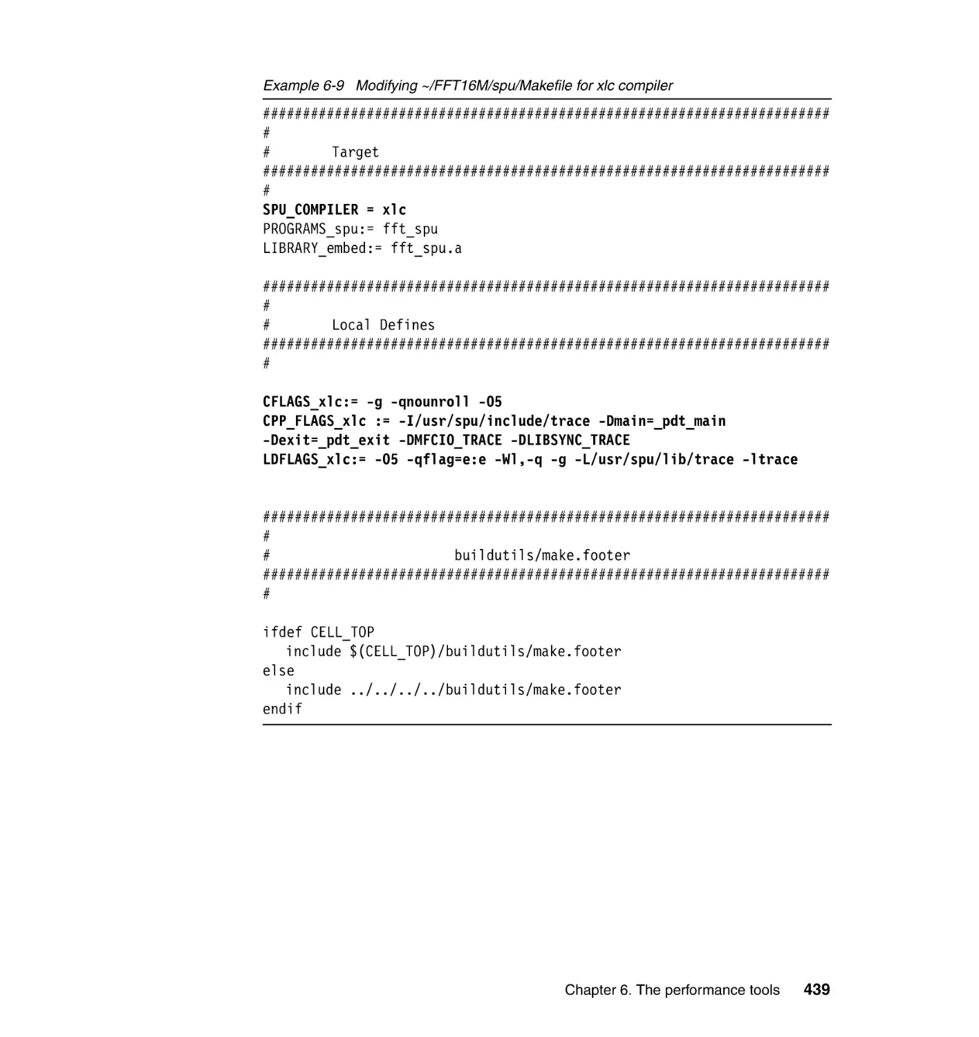
6.4.1 Step 1: Collecting trace data with PDT . . . . . . . . . . . . . . . . . . . . . . 438
6.4.2 Step 2: Importing the PDT data into Trace Analyzer. . . . . . . . . . . . 441
Chapter 7. Programming in distributed environments . . . . . . . . . . . . . . 445
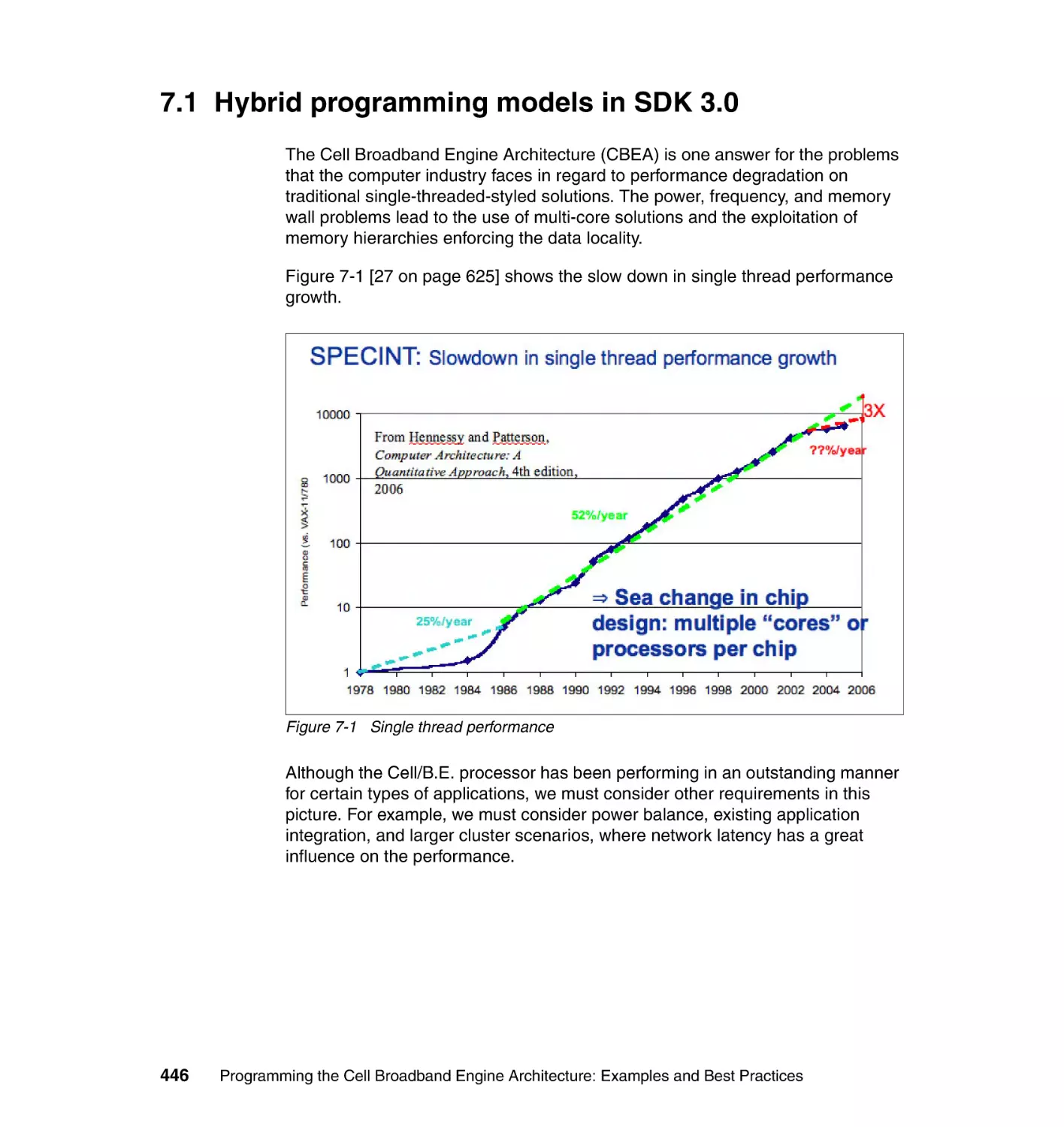
7.1 Hybrid programming models in SDK 3.0 . . . . . . . . . . . . . . . . . . . . . . . . . 446
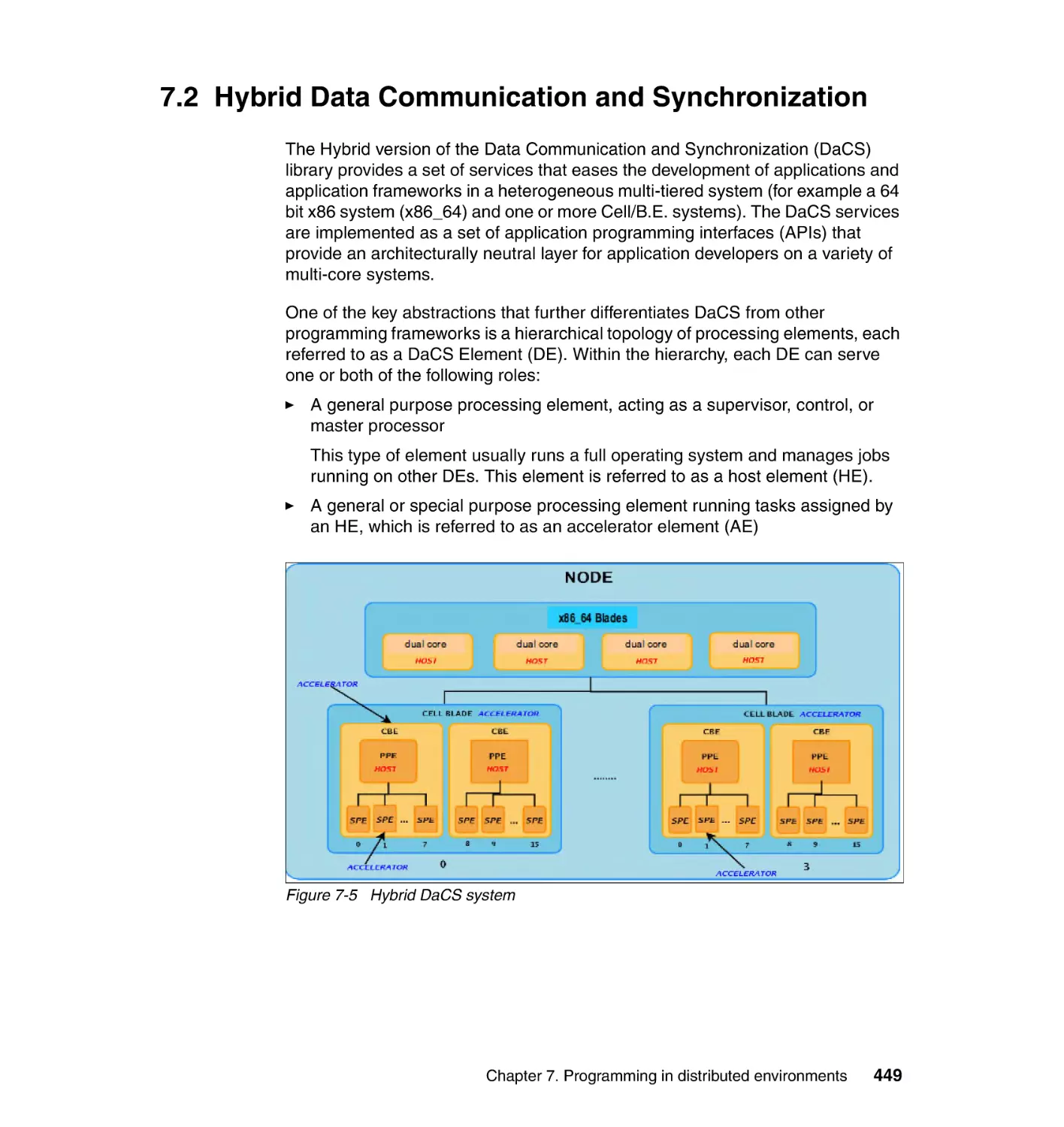
7.2 Hybrid Data Communication and Synchronization . . . . . . . . . . . . . . . . . 449
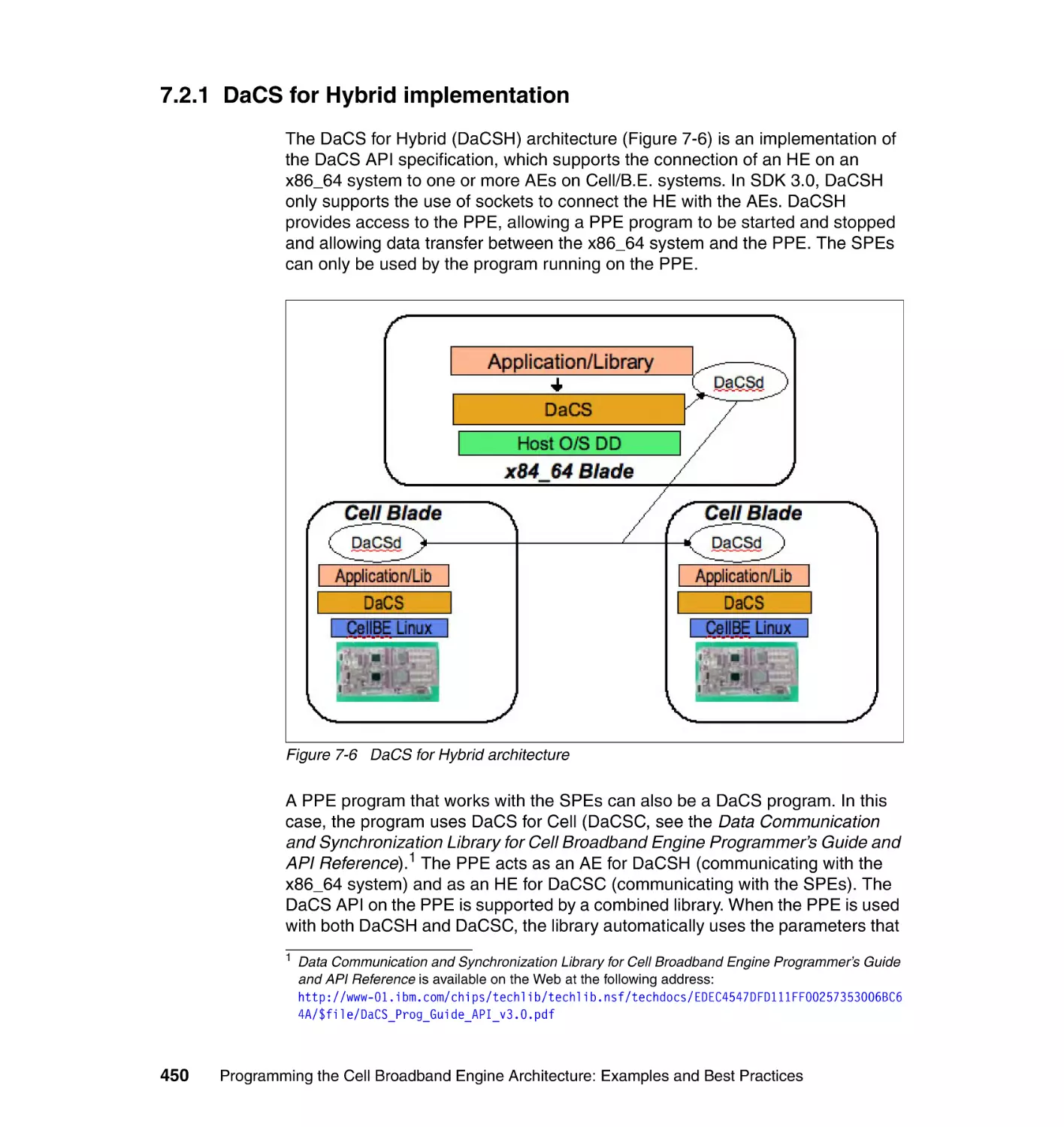
7.2.1 DaCS for Hybrid implementation. . . . . . . . . . . . . . . . . . . . . . . . . . . 450
7.2.2 Programming considerations . . . . . . . . . . . . . . . . . . . . . . . . . . . . . 452
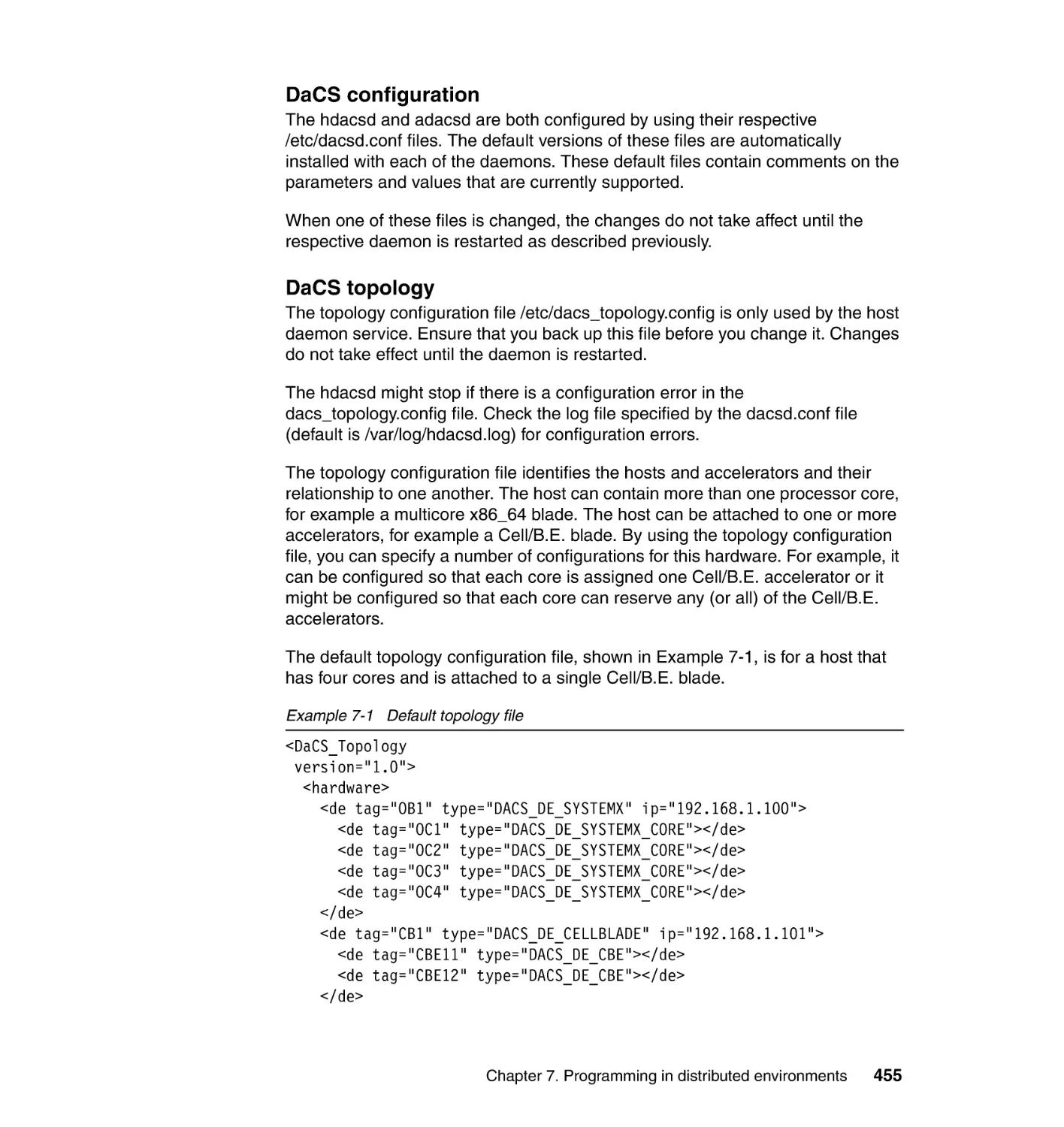
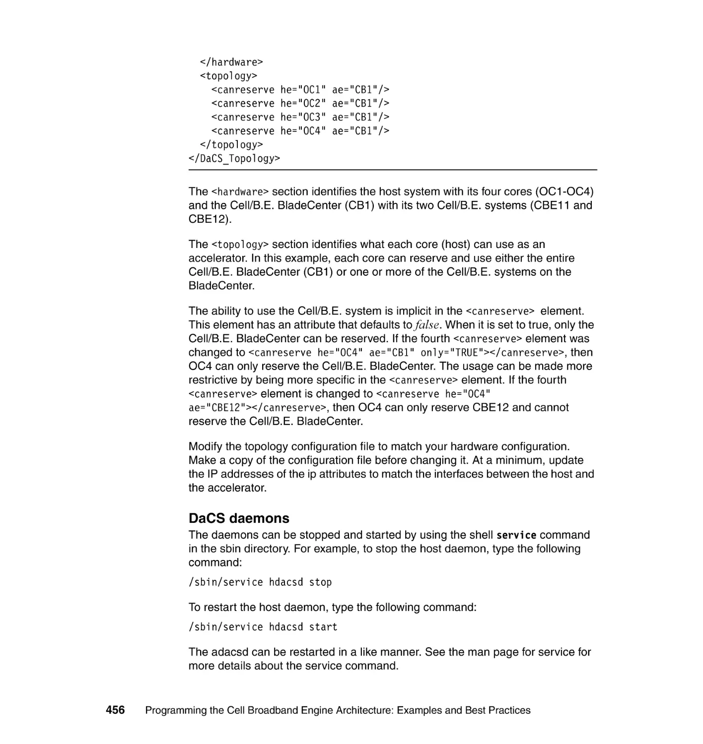
7.2.3 Building and running a Hybrid DaCS application . . . . . . . . . . . . . . 454
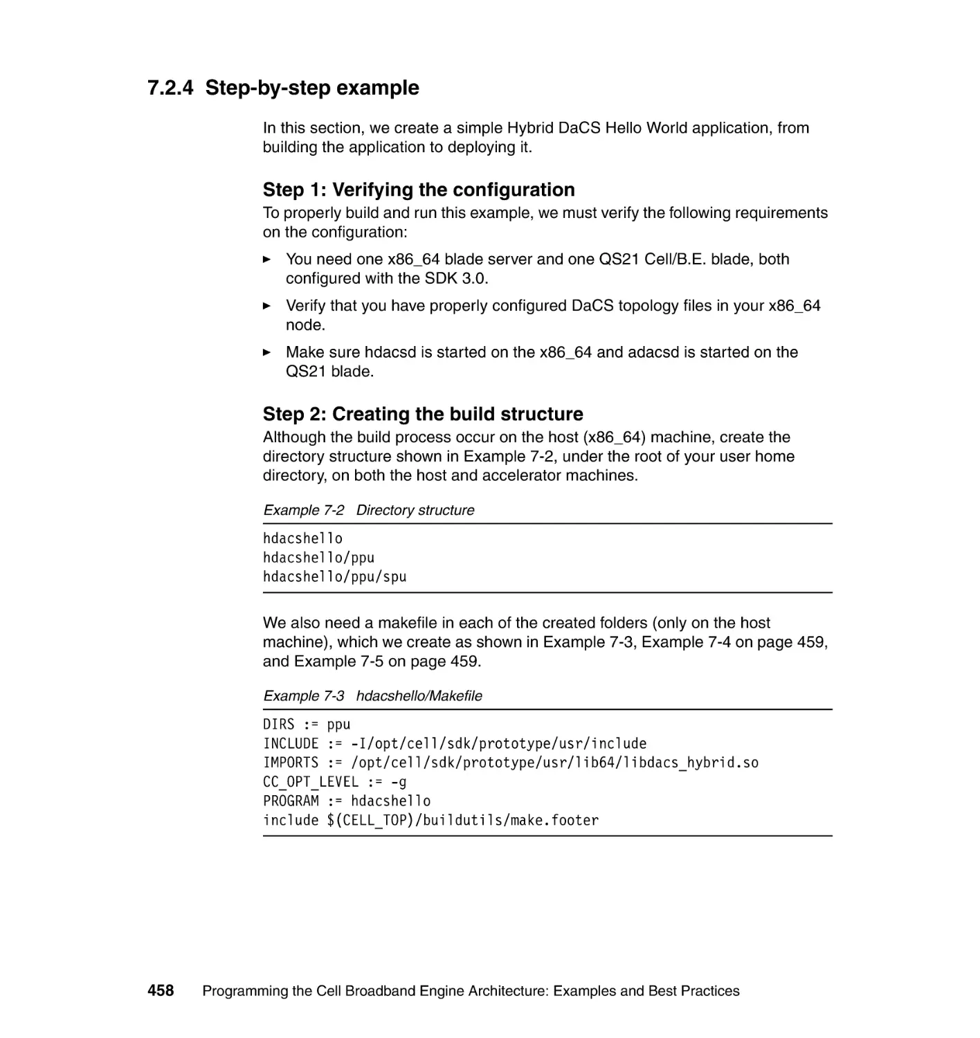
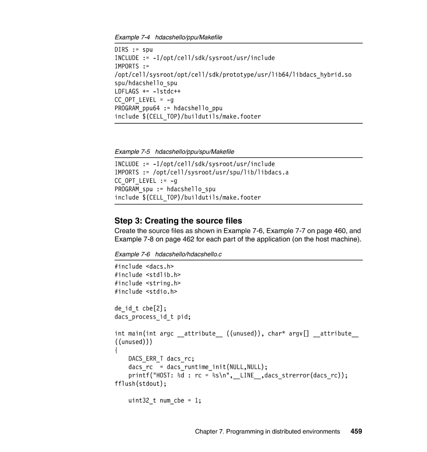
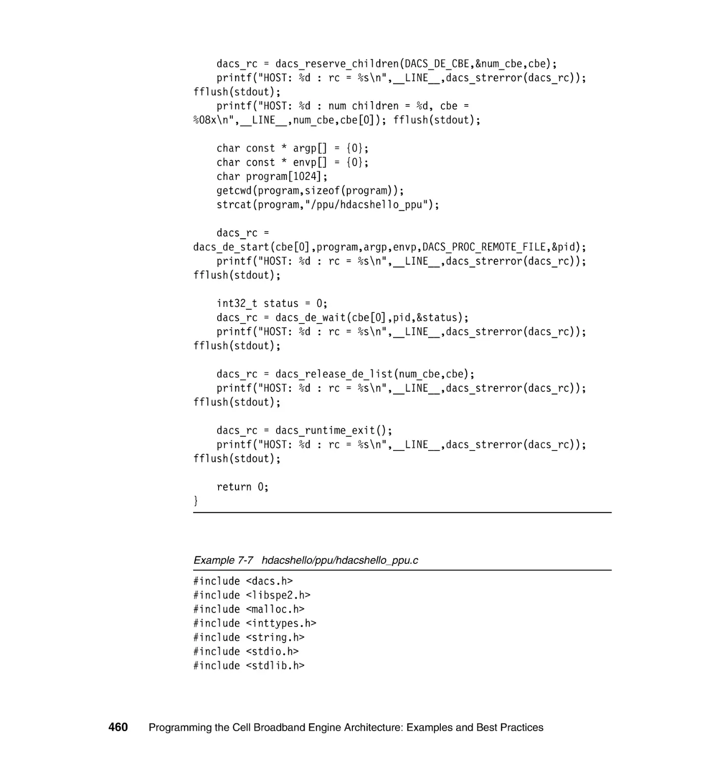
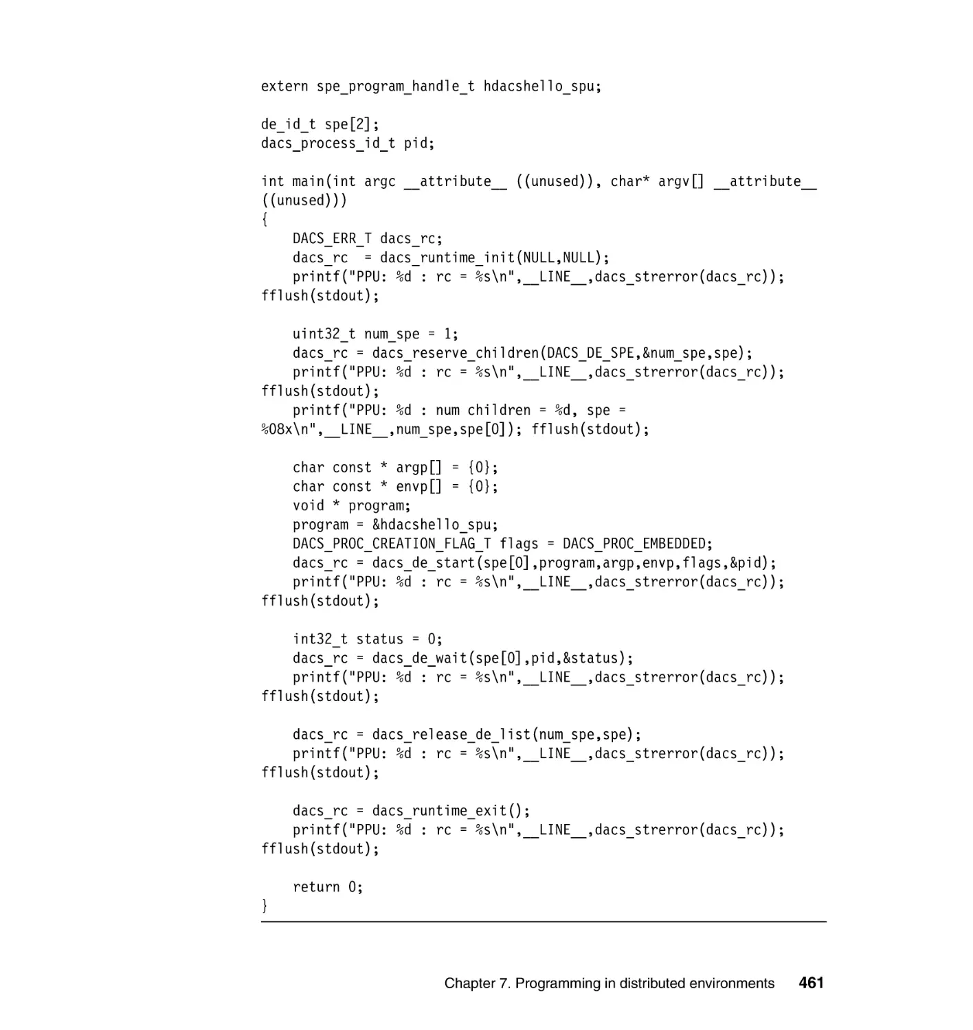
7.2.4 Step-by-step example . . . . . . . . . . . . . . . . . . . . . . . . . . . . . . . . . . . 458
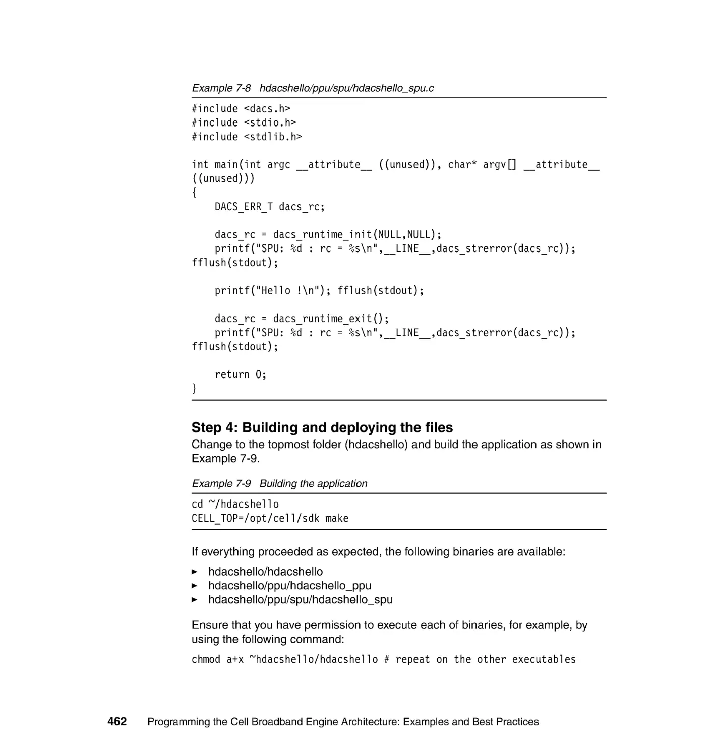
7.3 Hybrid ALF . . . . . . . . . . . . . . . . . . . . . . . . . . . . . . . . . . . . . . . . . . . . . . . 463
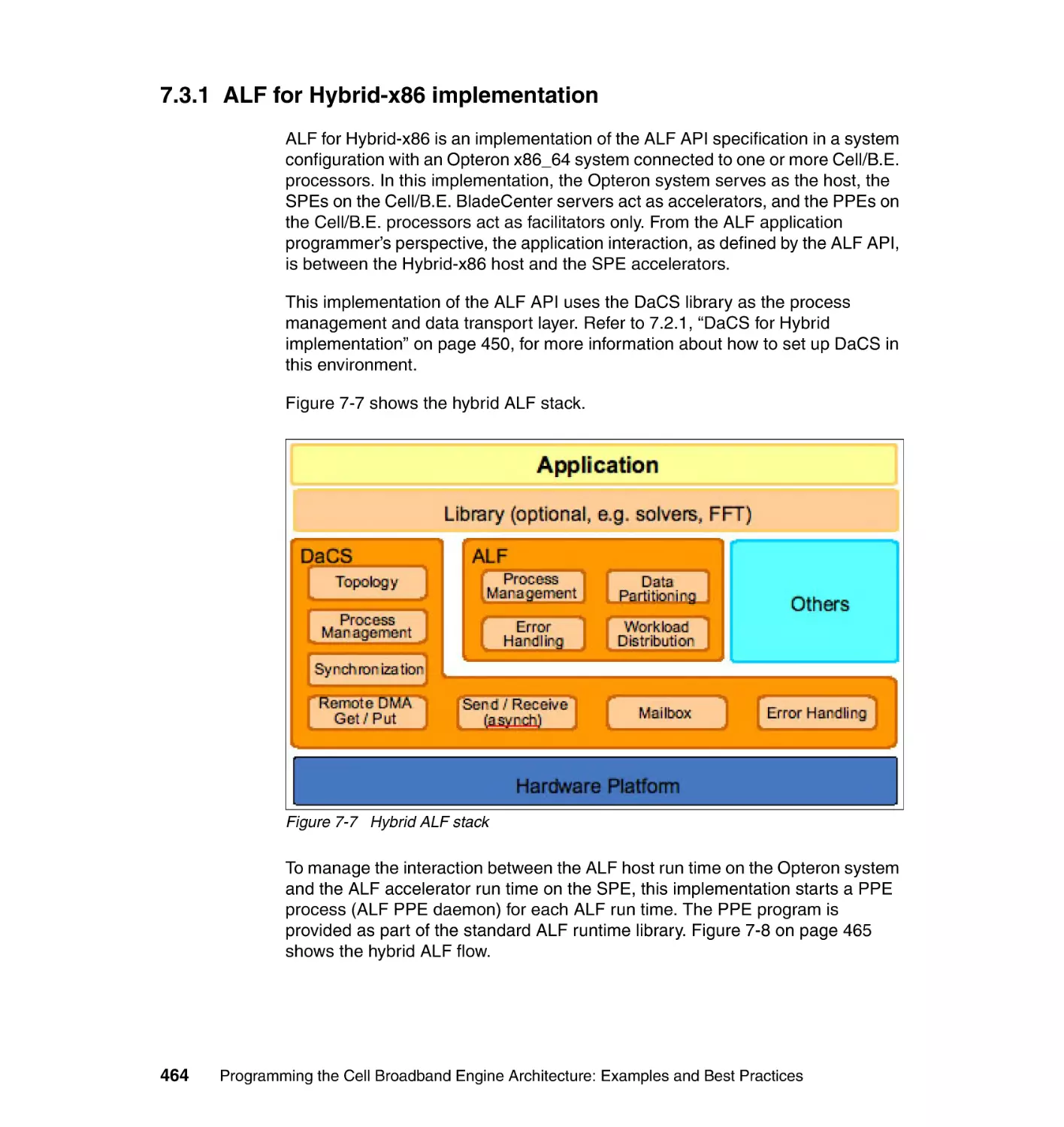
7.3.1 ALF for Hybrid-x86 implementation. . . . . . . . . . . . . . . . . . . . . . . . . 464
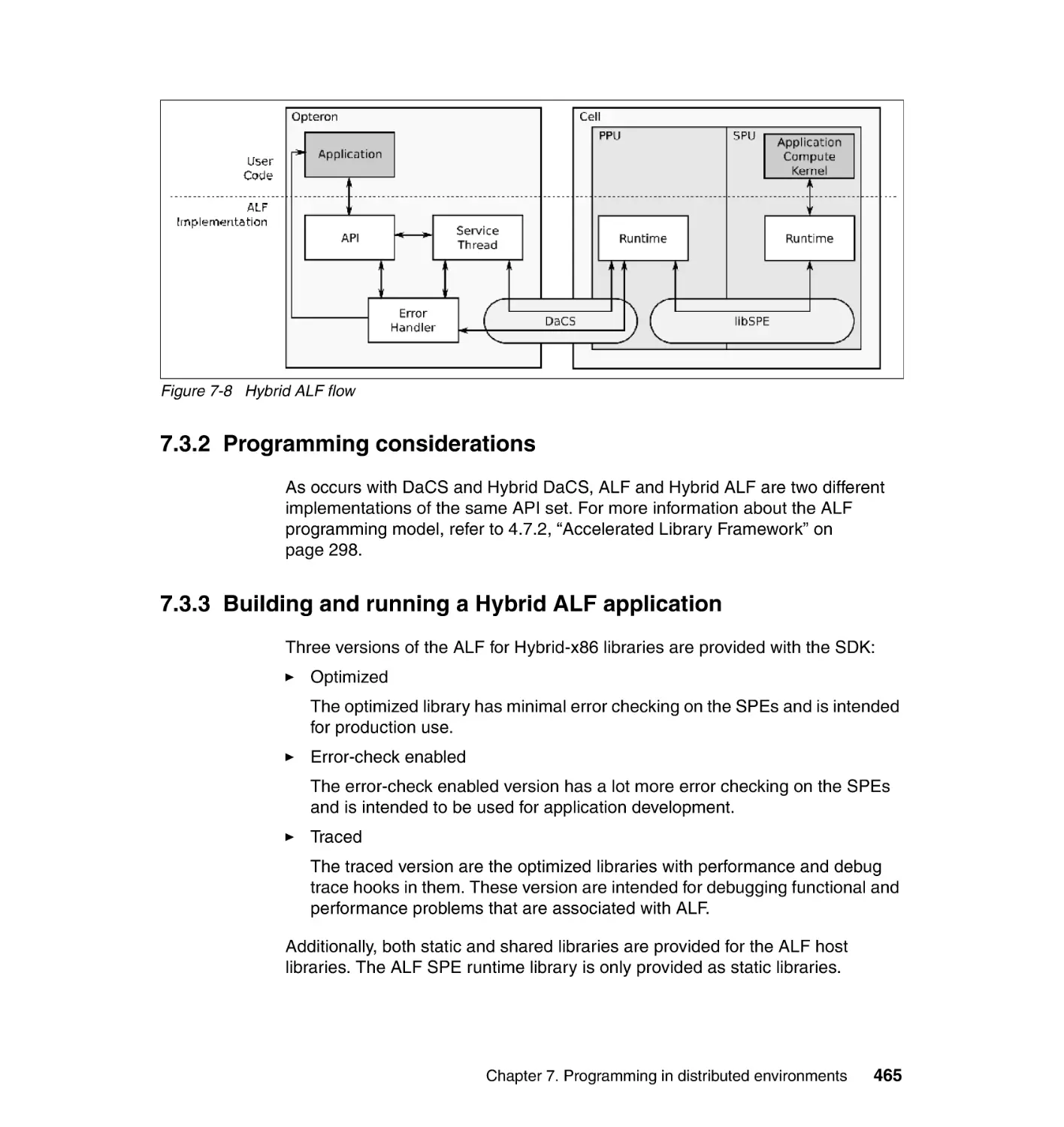
7.3.2 Programming considerations . . . . . . . . . . . . . . . . . . . . . . . . . . . . . 465
7.3.3 Building and running a Hybrid ALF application . . . . . . . . . . . . . . . . 465
7.3.4 Running a Hybrid ALF application. . . . . . . . . . . . . . . . . . . . . . . . . . 466
7.3.5 Step-by-step example . . . . . . . . . . . . . . . . . . . . . . . . . . . . . . . . . . . 467
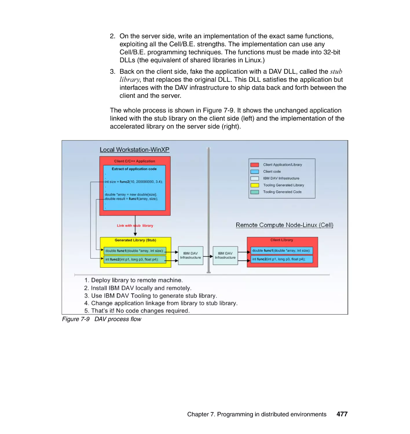
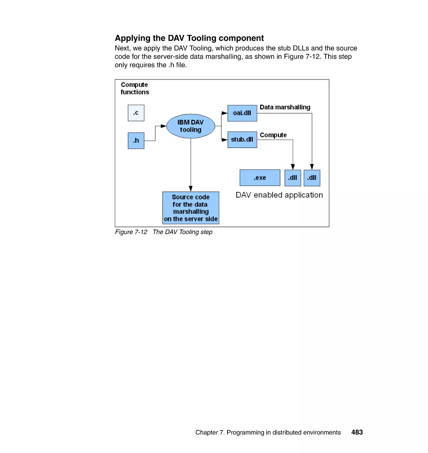
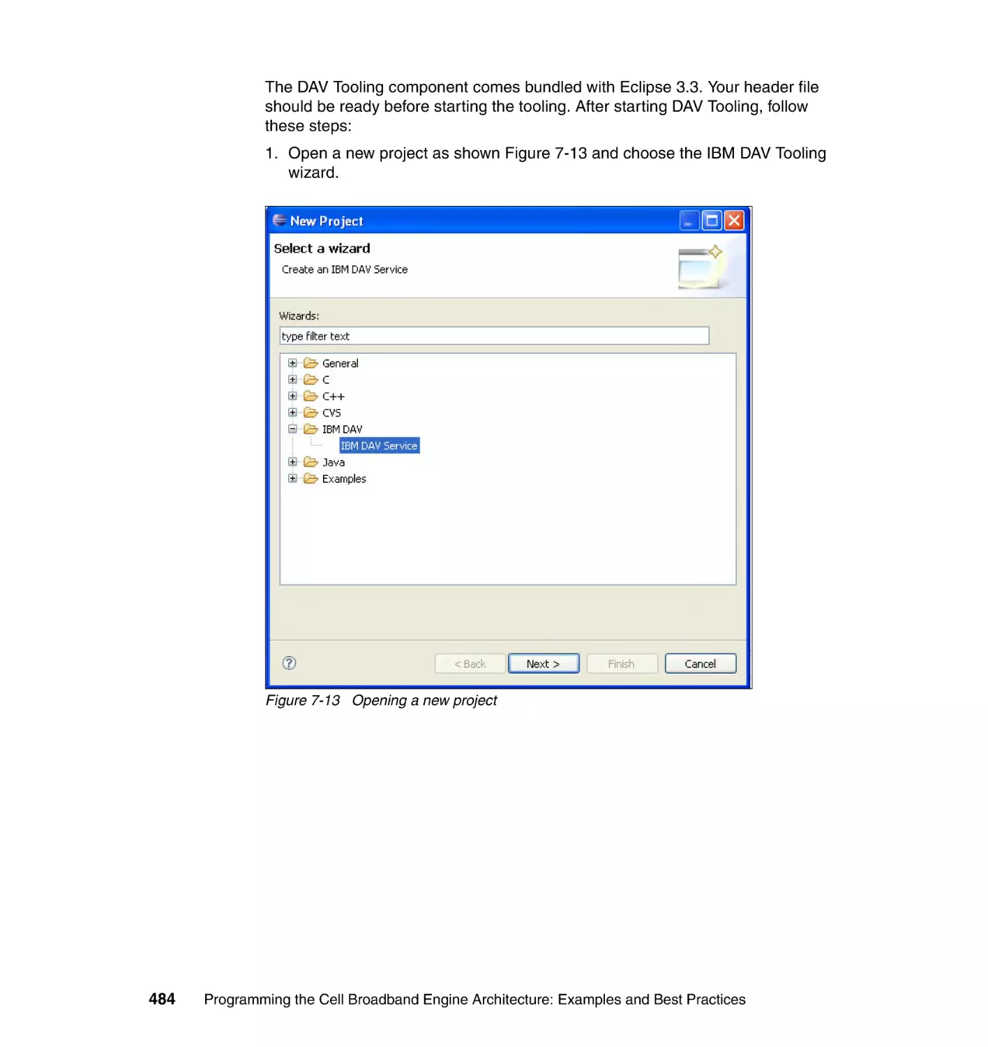
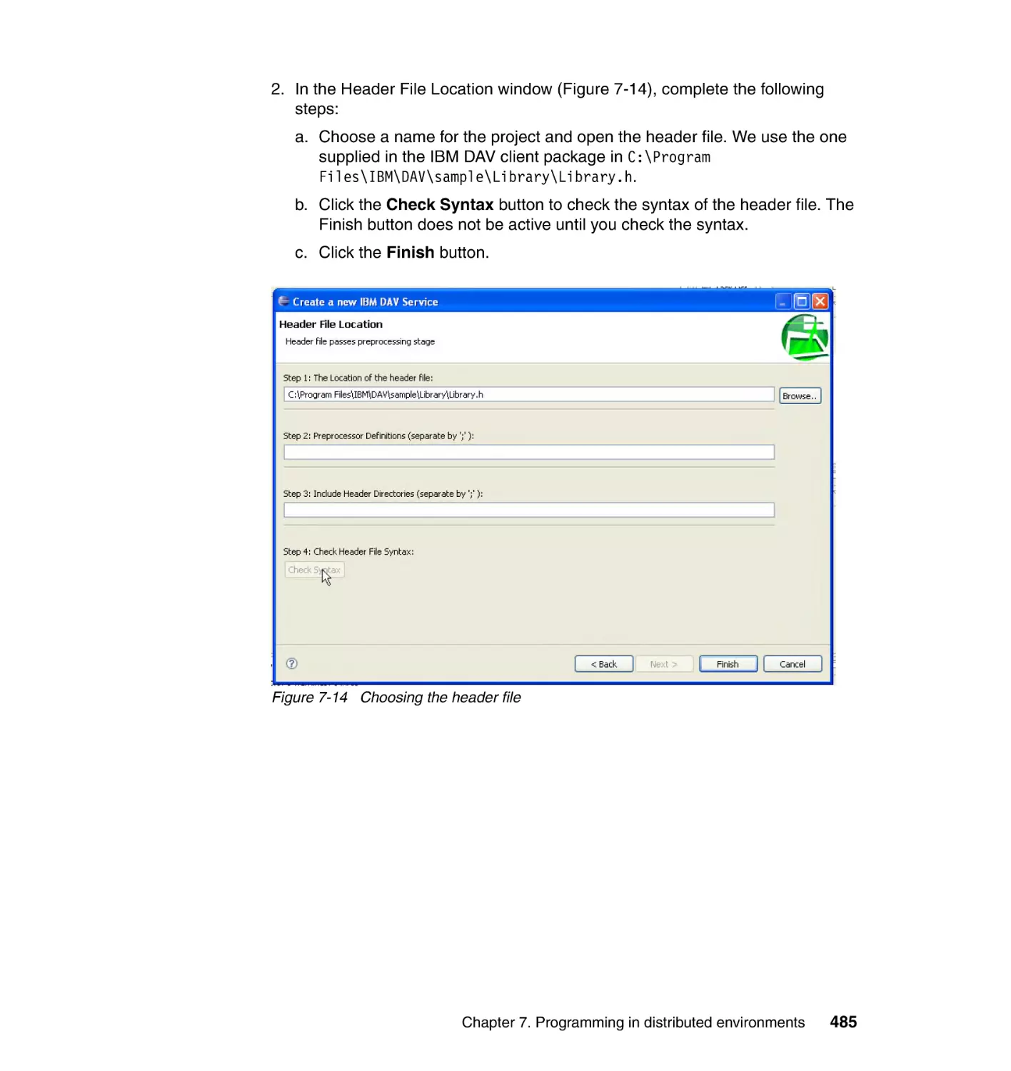
7.4 Dynamic Application Virtualization . . . . . . . . . . . . . . . . . . . . . . . . . . . . . 475
7.4.1 DAV target applications. . . . . . . . . . . . . . . . . . . . . . . . . . . . . . . . . . 476
7.4.2 DAV architecture . . . . . . . . . . . . . . . . . . . . . . . . . . . . . . . . . . . . . . . 476
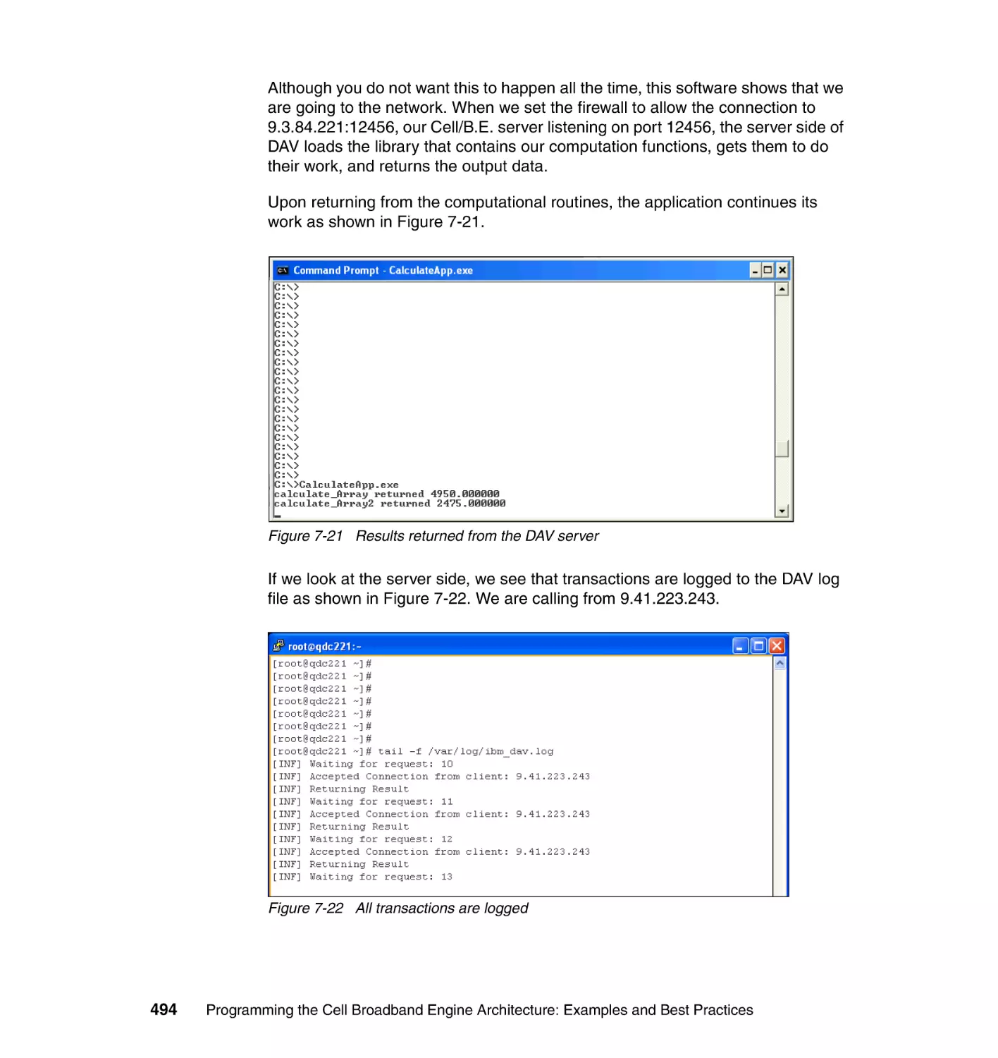
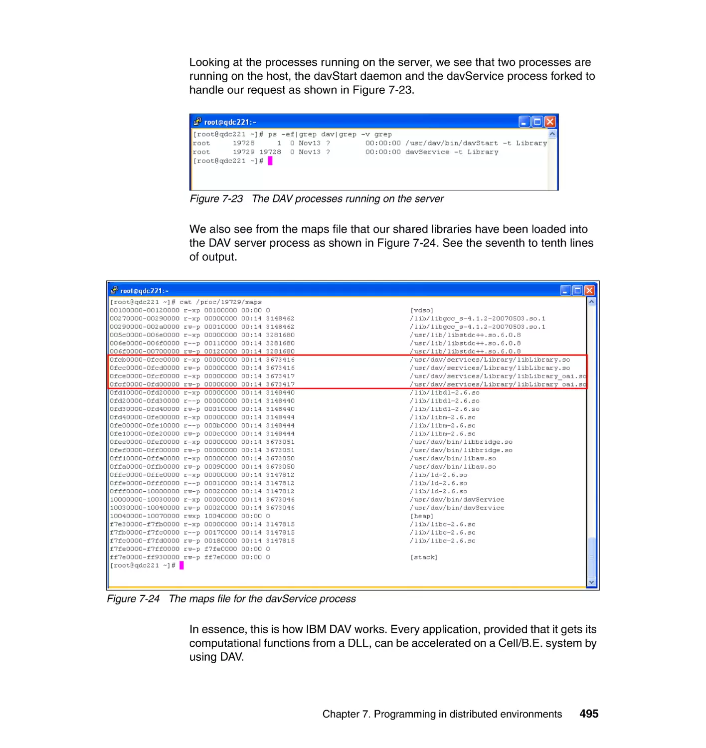
7.4.3 Running a DAV-enabled application . . . . . . . . . . . . . . . . . . . . . . . . 478
7.4.4 System requirements . . . . . . . . . . . . . . . . . . . . . . . . . . . . . . . . . . . 478
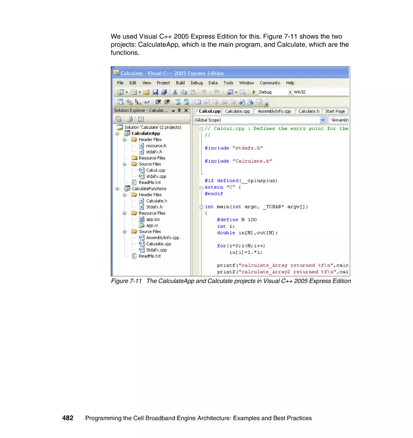
7.4.5 A Visual C++ application example . . . . . . . . . . . . . . . . . . . . . . . . . 479
7.4.6 Visual Basic example: An Excel 2007 spreadsheet . . . . . . . . . . . . 496
Contents
vii
Part 3. Application re-engineering . . . . . . . . . . . . . . . . . . . . . . . . . . . . . . . . . . . . . . . . . . . 497
Chapter 8. Case study: Monte Carlo simulation. . . . . . . . . . . . . . . . . . . . 499
8.1 Monte Carlo simulation for option pricing . . . . . . . . . . . . . . . . . . . . . . . . 500
8.2 Methods to generate Gaussian (normal) random variables . . . . . . . . . . 502
8.3 Parallel and vector implementation of the Monte Carlo algorithm on the
Cell/B.E. architecture . . . . . . . . . . . . . . . . . . . . . . . . . . . . . . . . . . . . . . . 503
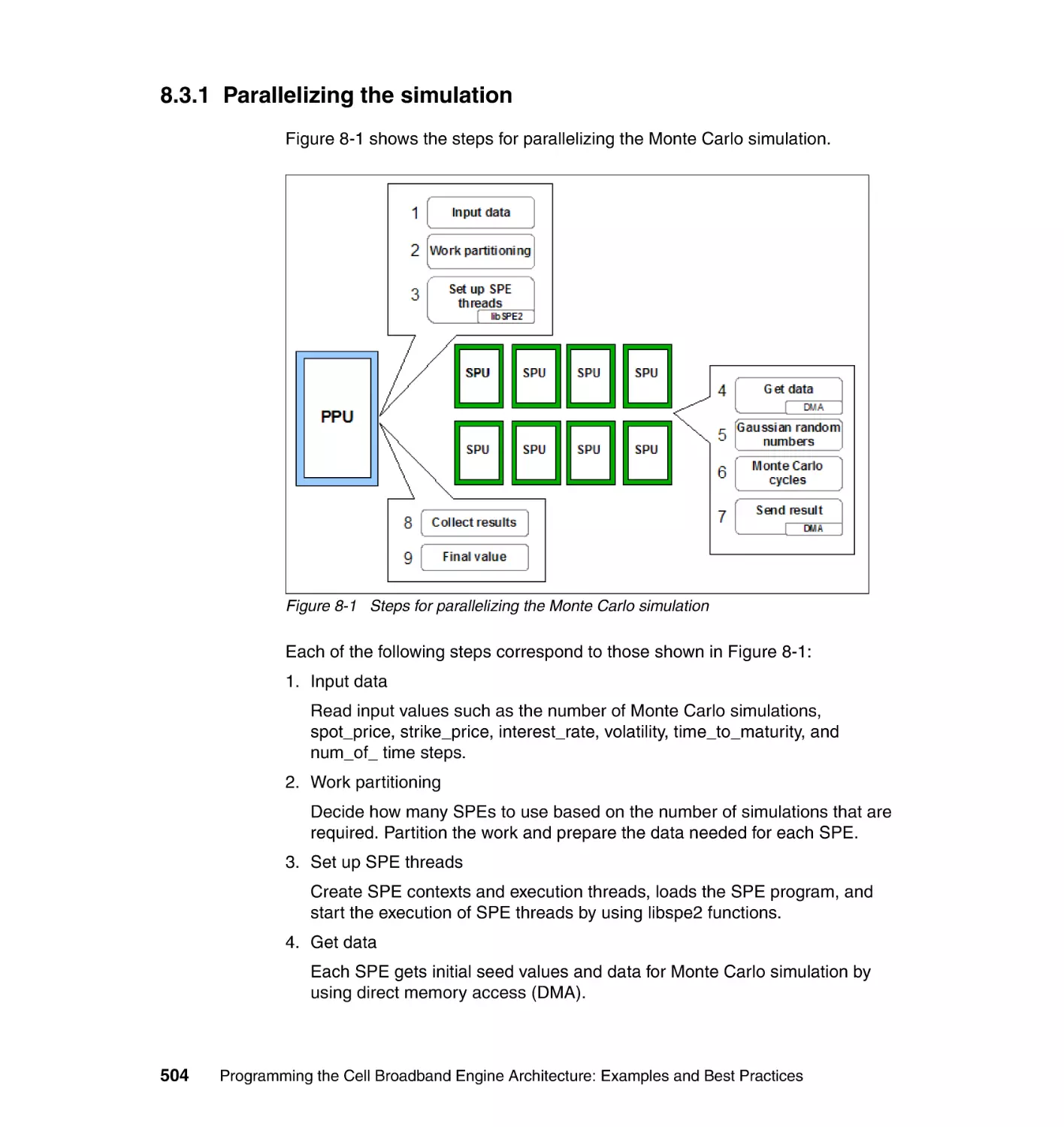
8.3.1 Parallelizing the simulation . . . . . . . . . . . . . . . . . . . . . . . . . . . . . . . 504
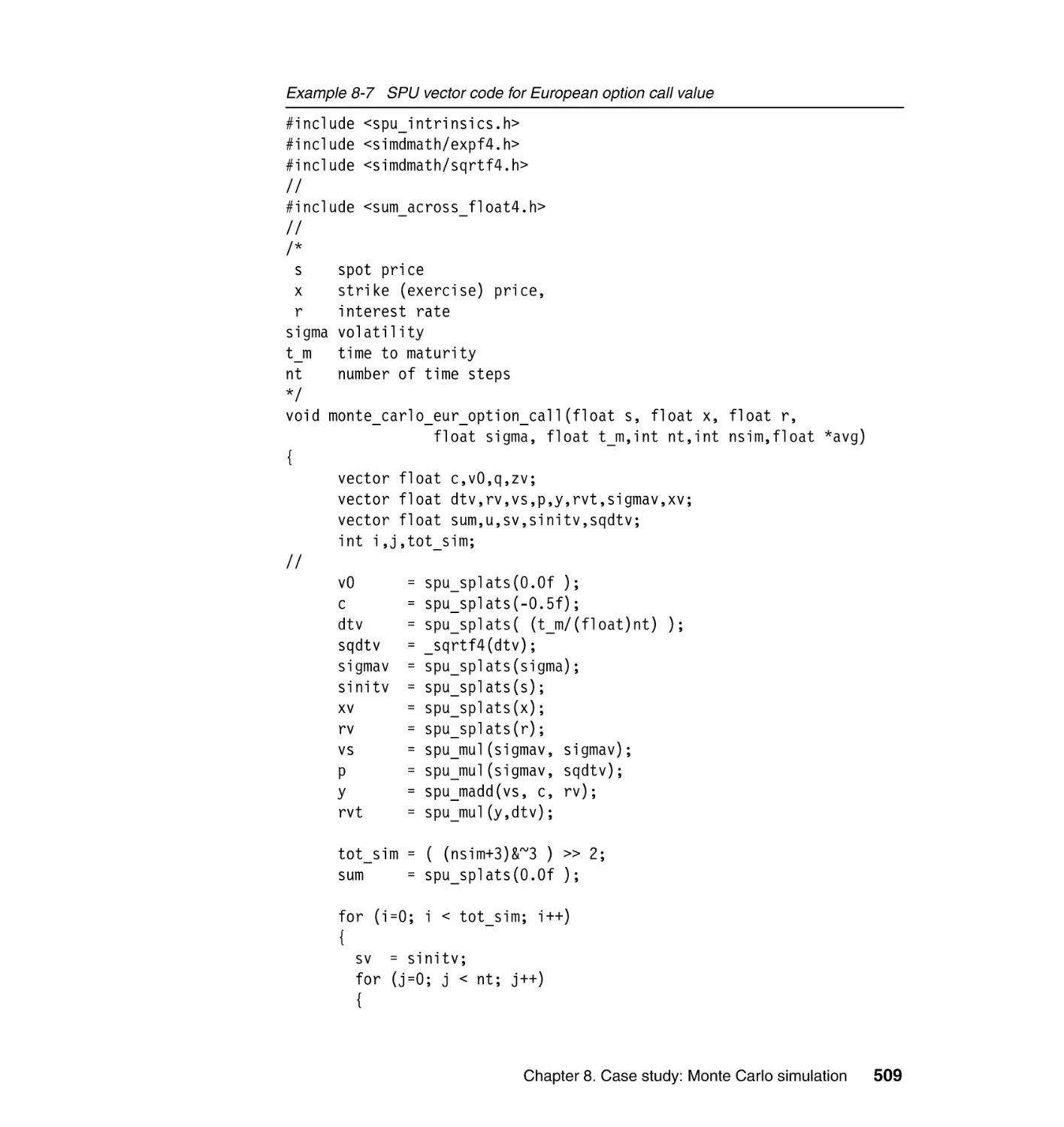
8.3.2 Sample code for a European option on the SPU . . . . . . . . . . . . . . 508
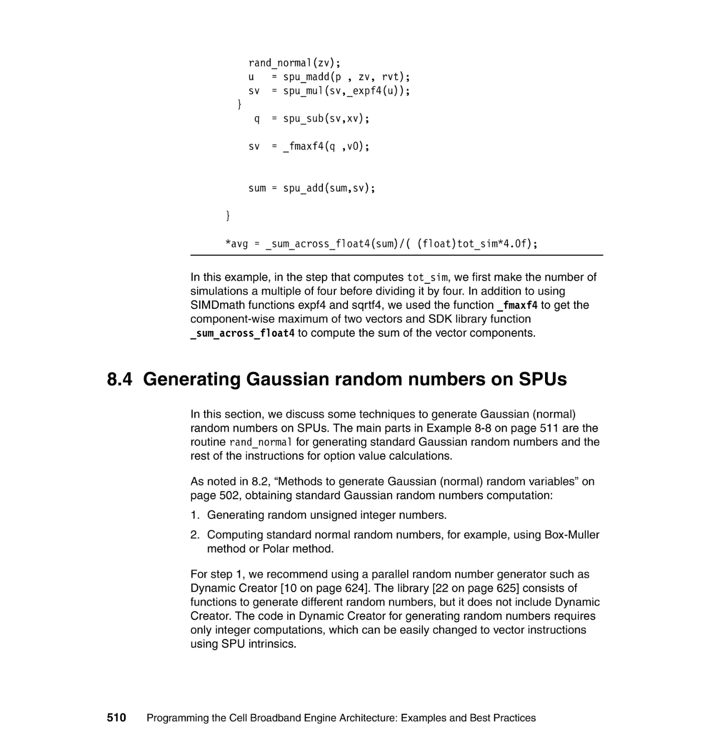
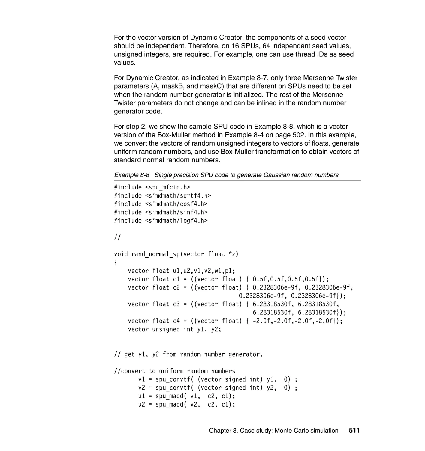
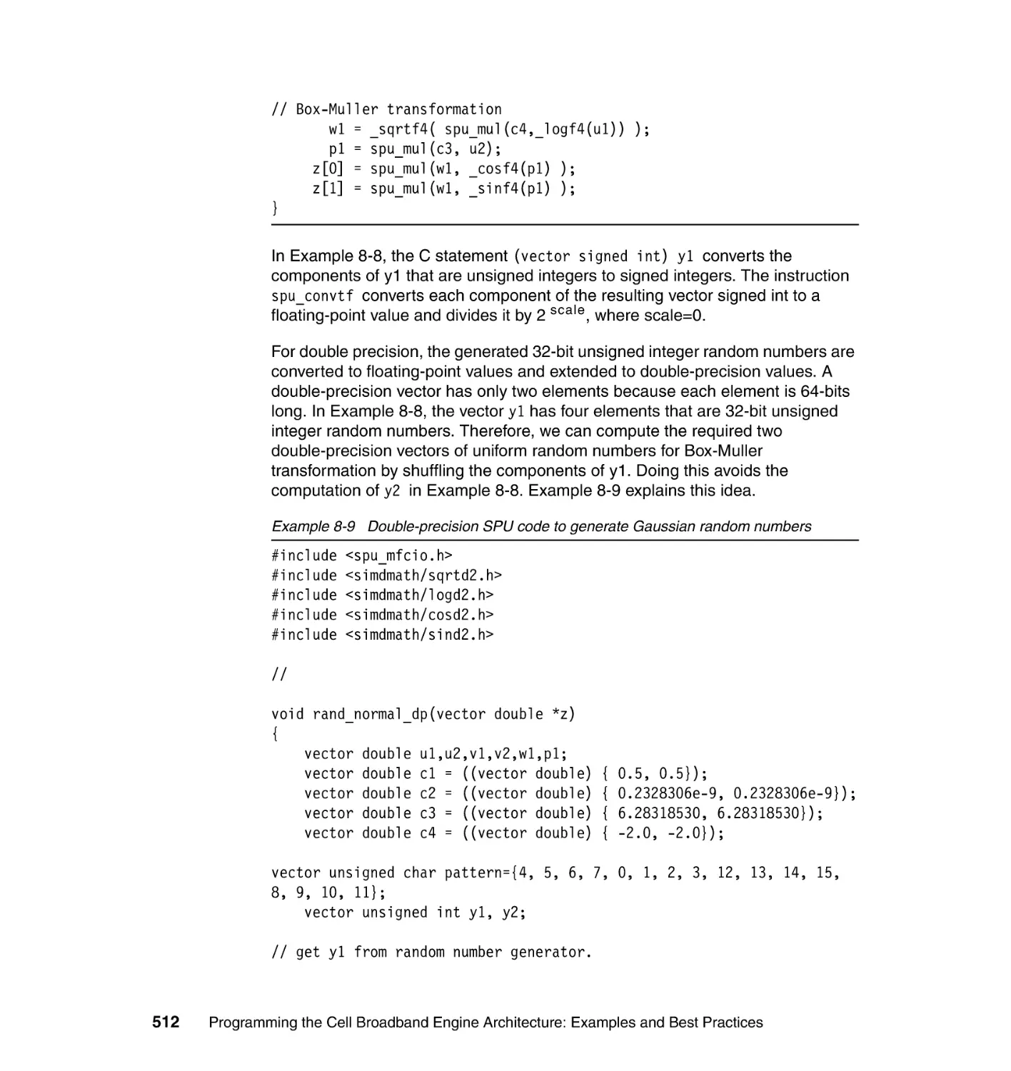
8.4 Generating Gaussian random numbers on SPUs . . . . . . . . . . . . . . . . . . 510
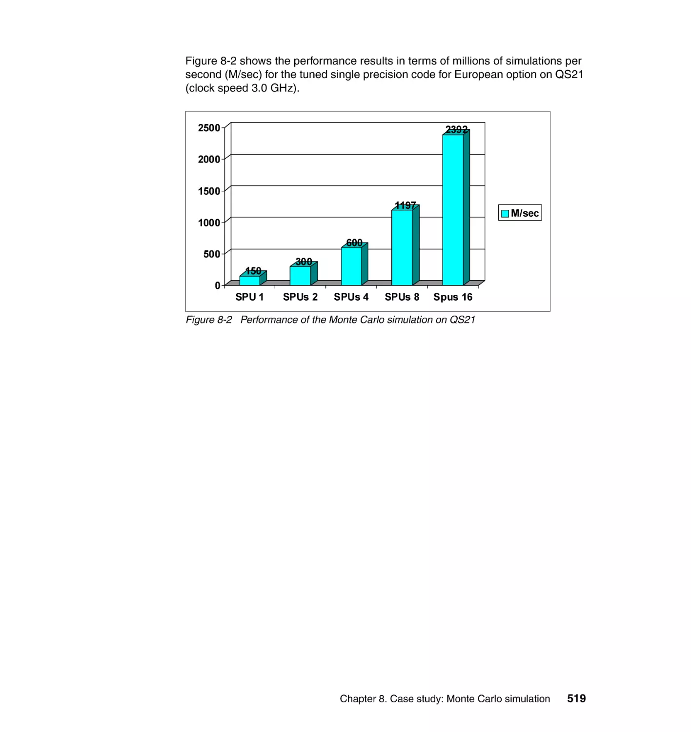
8.5 Improving the performance . . . . . . . . . . . . . . . . . . . . . . . . . . . . . . . . . . . 518
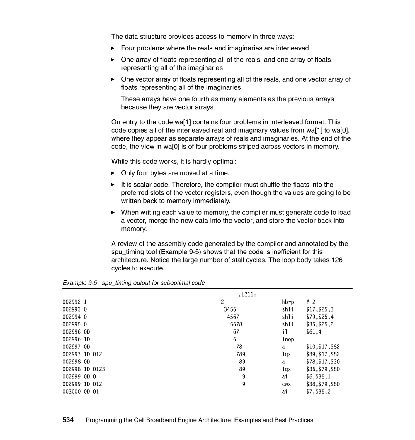
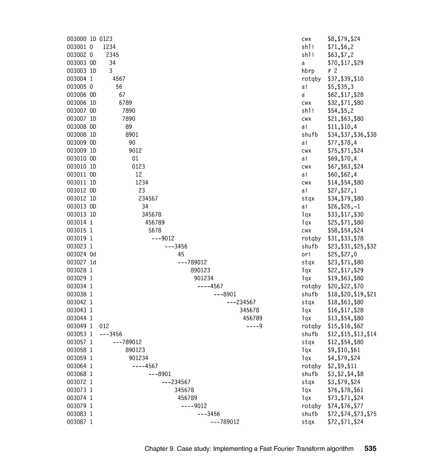
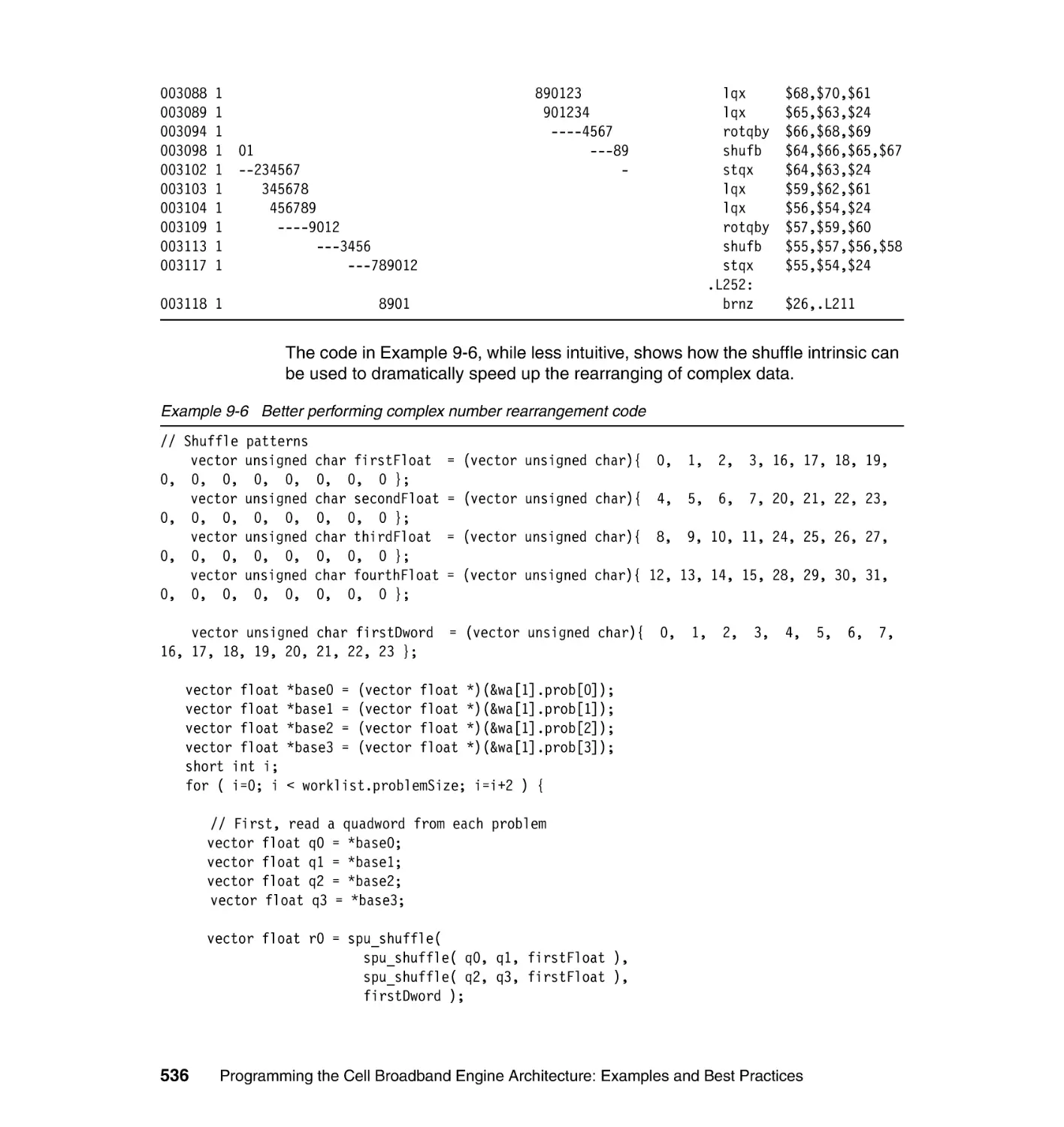
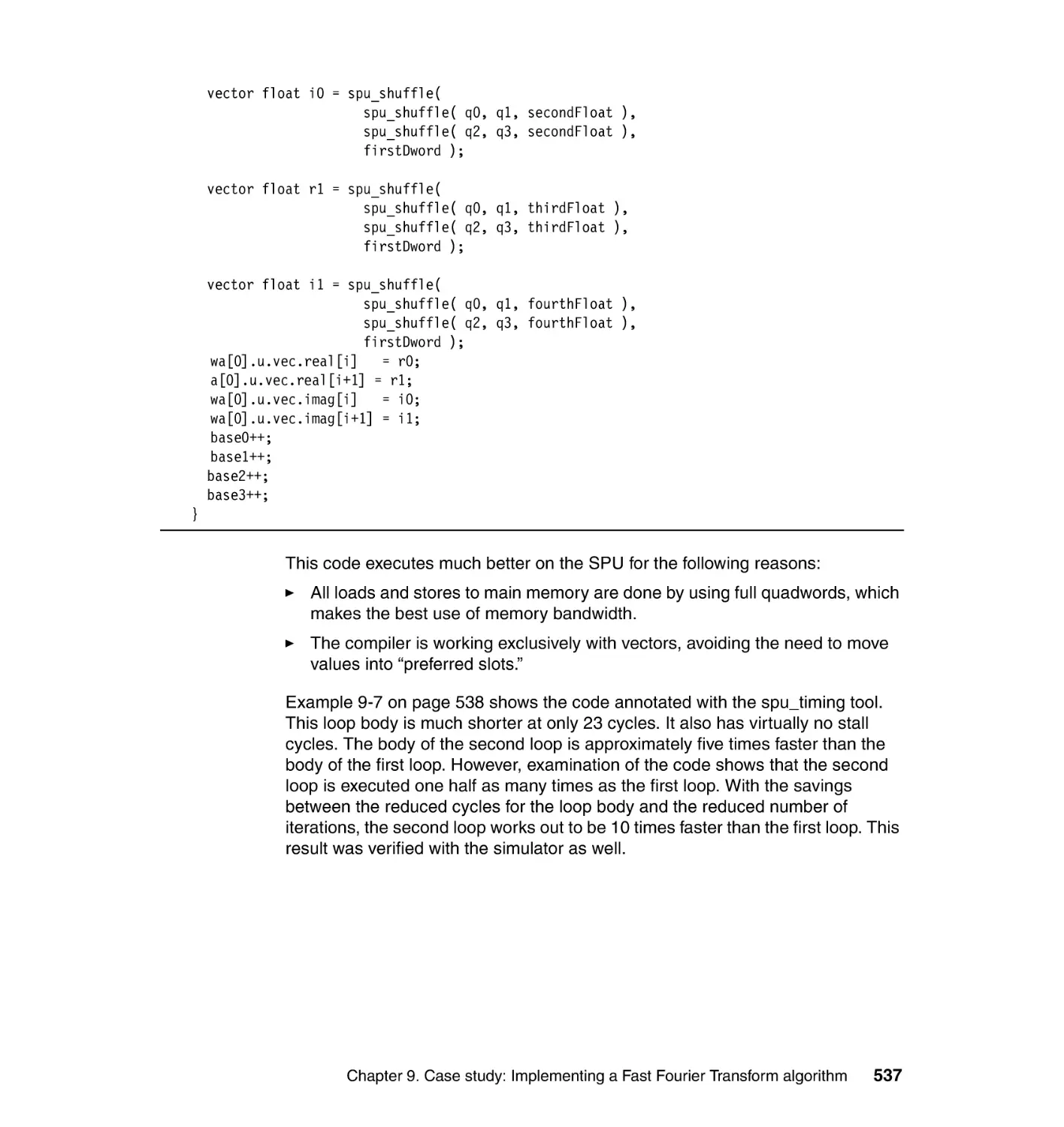
Chapter 9. Case study: Implementing a Fast Fourier Transform
algorithm . . . . . . . . . . . . . . . . . . . . . . . . . . . . . . . . . . . . . . . . . . 521
9.1 Motivation for an FFT algorithm . . . . . . . . . . . . . . . . . . . . . . . . . . . . . . . 522
9.2 Development process . . . . . . . . . . . . . . . . . . . . . . . . . . . . . . . . . . . . . . . 522
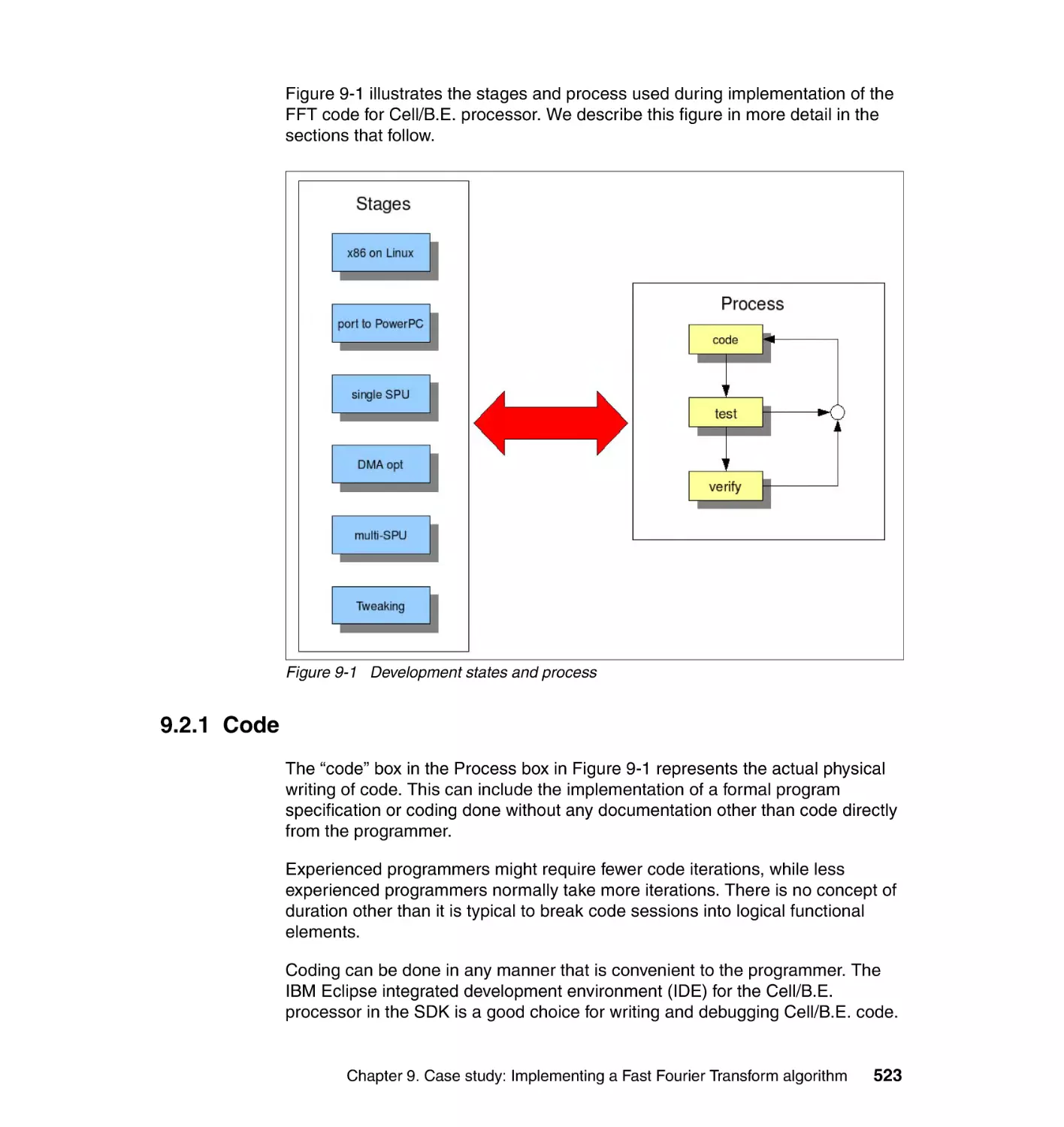
9.2.1 Code . . . . . . . . . . . . . . . . . . . . . . . . . . . . . . . . . . . . . . . . . . . . . . . . 523
9.2.2 Test . . . . . . . . . . . . . . . . . . . . . . . . . . . . . . . . . . . . . . . . . . . . . . . . . 524
9.2.3 Verify . . . . . . . . . . . . . . . . . . . . . . . . . . . . . . . . . . . . . . . . . . . . . . . . 524
9.3 Development stages . . . . . . . . . . . . . . . . . . . . . . . . . . . . . . . . . . . . . . . . 526
9.3.1 x86 implementation . . . . . . . . . . . . . . . . . . . . . . . . . . . . . . . . . . . . . 526
9.3.2 Port to PowerPC . . . . . . . . . . . . . . . . . . . . . . . . . . . . . . . . . . . . . . . 526
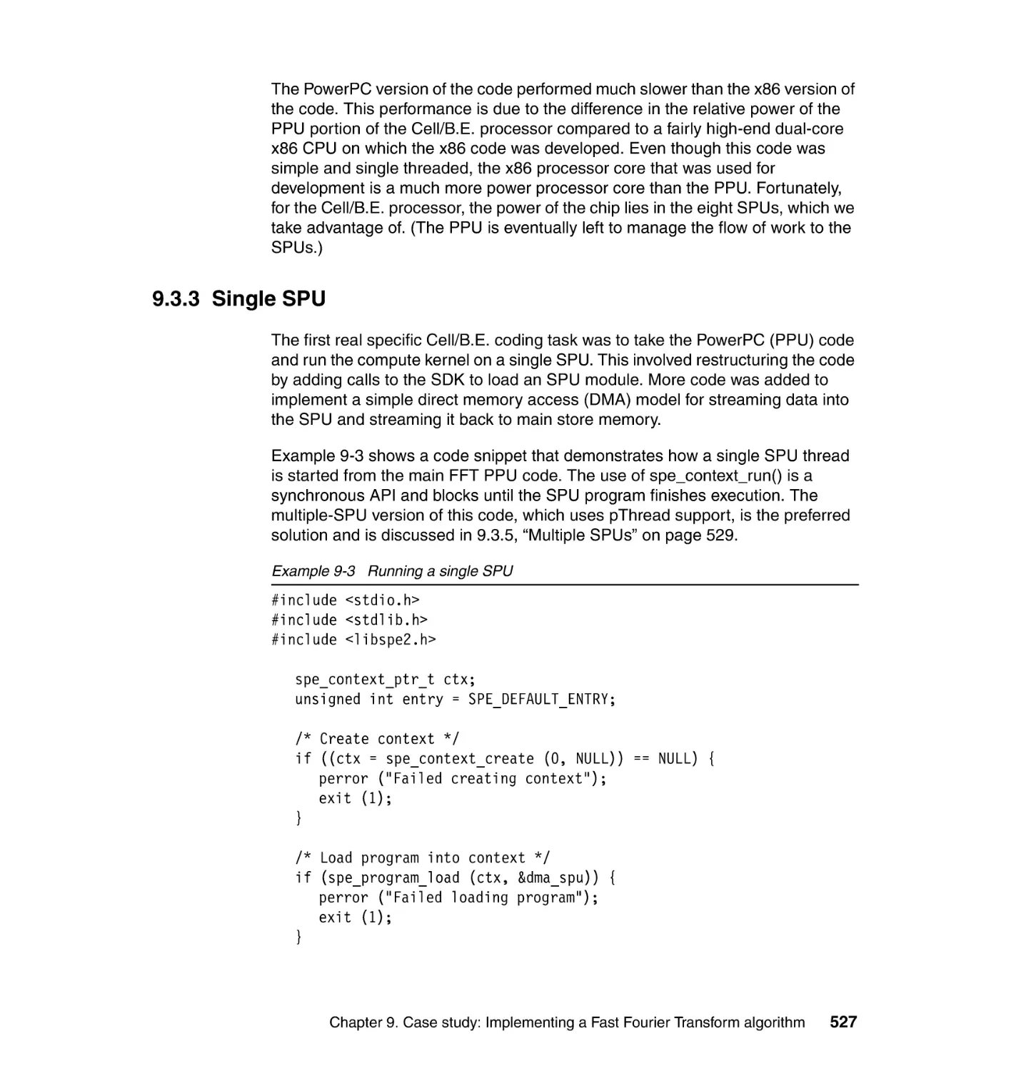
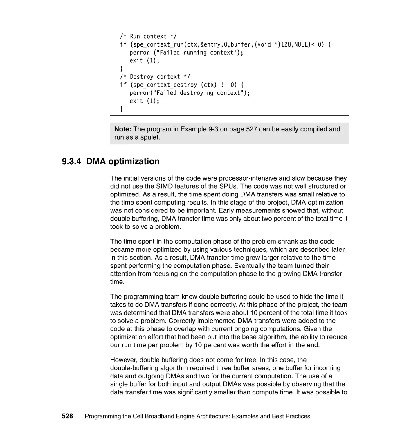
9.3.3 Single SPU . . . . . . . . . . . . . . . . . . . . . . . . . . . . . . . . . . . . . . . . . . . 527
9.3.4 DMA optimization . . . . . . . . . . . . . . . . . . . . . . . . . . . . . . . . . . . . . . 528
9.3.5 Multiple SPUs . . . . . . . . . . . . . . . . . . . . . . . . . . . . . . . . . . . . . . . . . 529
9.4 Strategies for using SIMD . . . . . . . . . . . . . . . . . . . . . . . . . . . . . . . . . . . . 529
9.4.1 Striping multiple problems across a vector . . . . . . . . . . . . . . . . . . . 530
9.4.2 Synthesizing vectors by loop unrolling . . . . . . . . . . . . . . . . . . . . . . 530
9.4.3 Measuring and tweaking performance . . . . . . . . . . . . . . . . . . . . . . 531
Part 4. Systems . . . . . . . . . . . . . . . . . . . . . . . . . . . . . . . . . . . . . . . . . . . . . . . . . . . . . . . . . . . 539
Chapter 10. SDK 3.0 and BladeCenter QS21 system configuration . . . . 541
10.1 BladeCenter QS21 characteristics . . . . . . . . . . . . . . . . . . . . . . . . . . . . 542
10.2 Installing the operating system . . . . . . . . . . . . . . . . . . . . . . . . . . . . . . . 543
10.2.1 Important considerations . . . . . . . . . . . . . . . . . . . . . . . . . . . . . . . . 543
10.2.2 Managing and accessing the blade server . . . . . . . . . . . . . . . . . . 544
10.2.3 Installation from network storage . . . . . . . . . . . . . . . . . . . . . . . . . 547
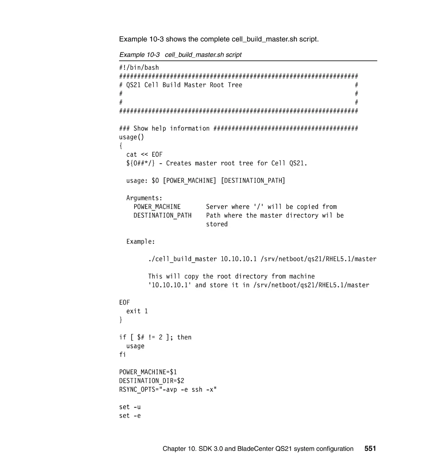
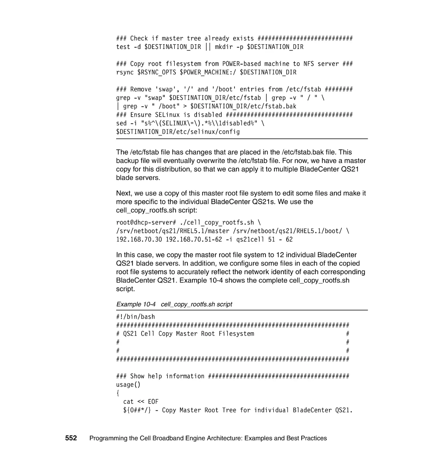
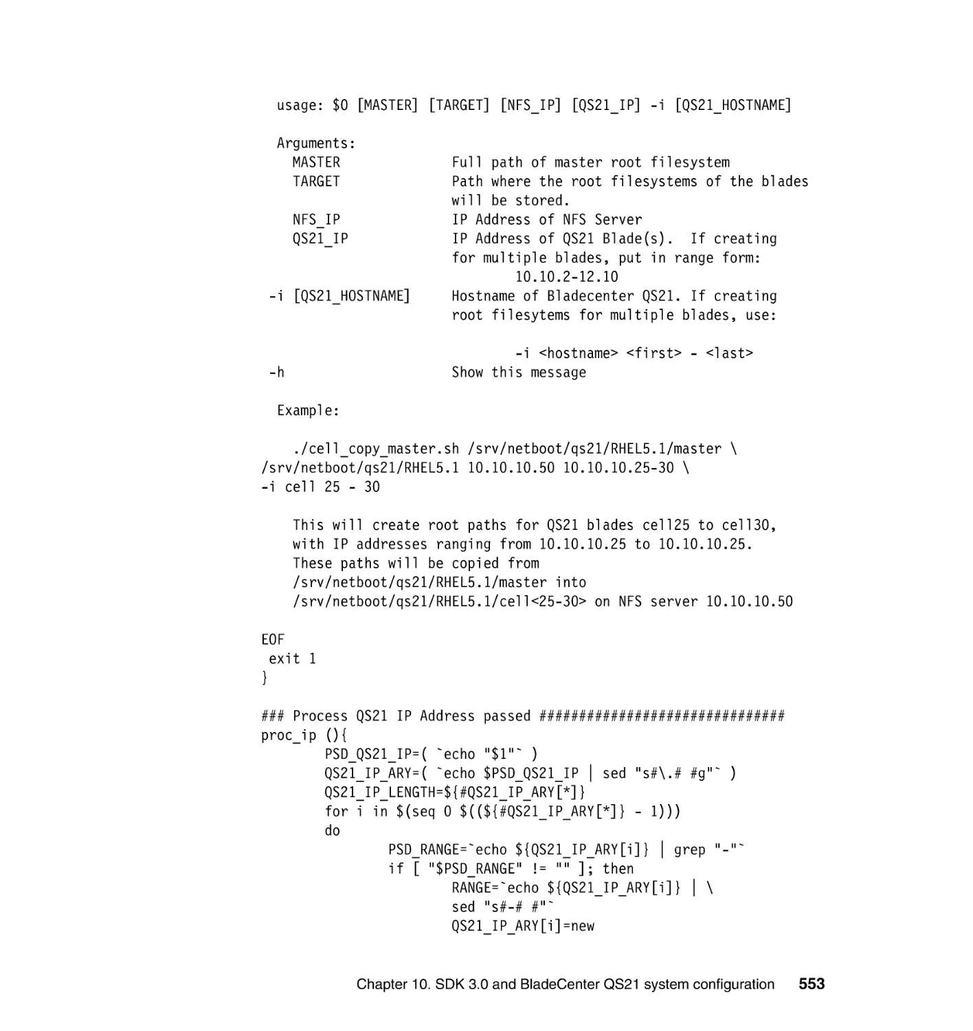
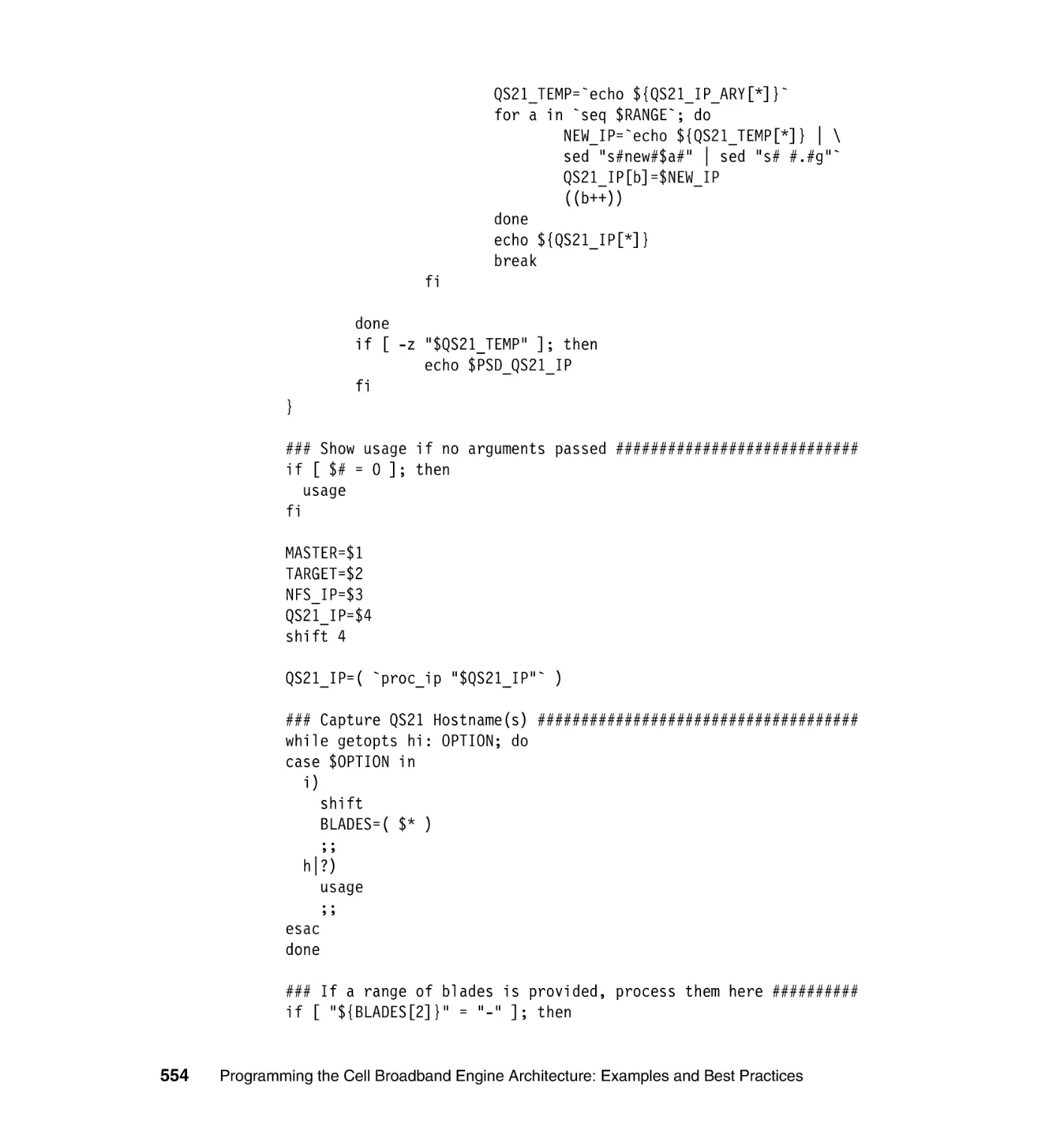
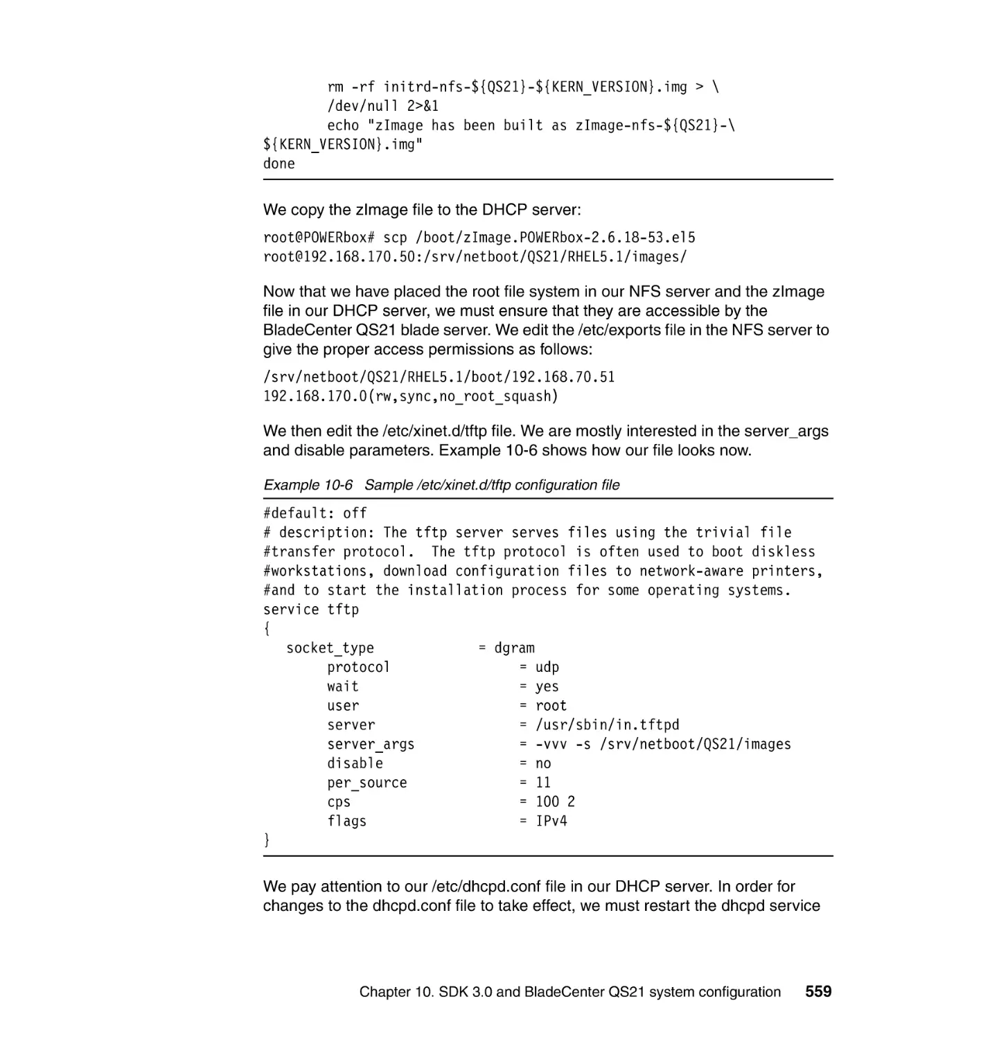
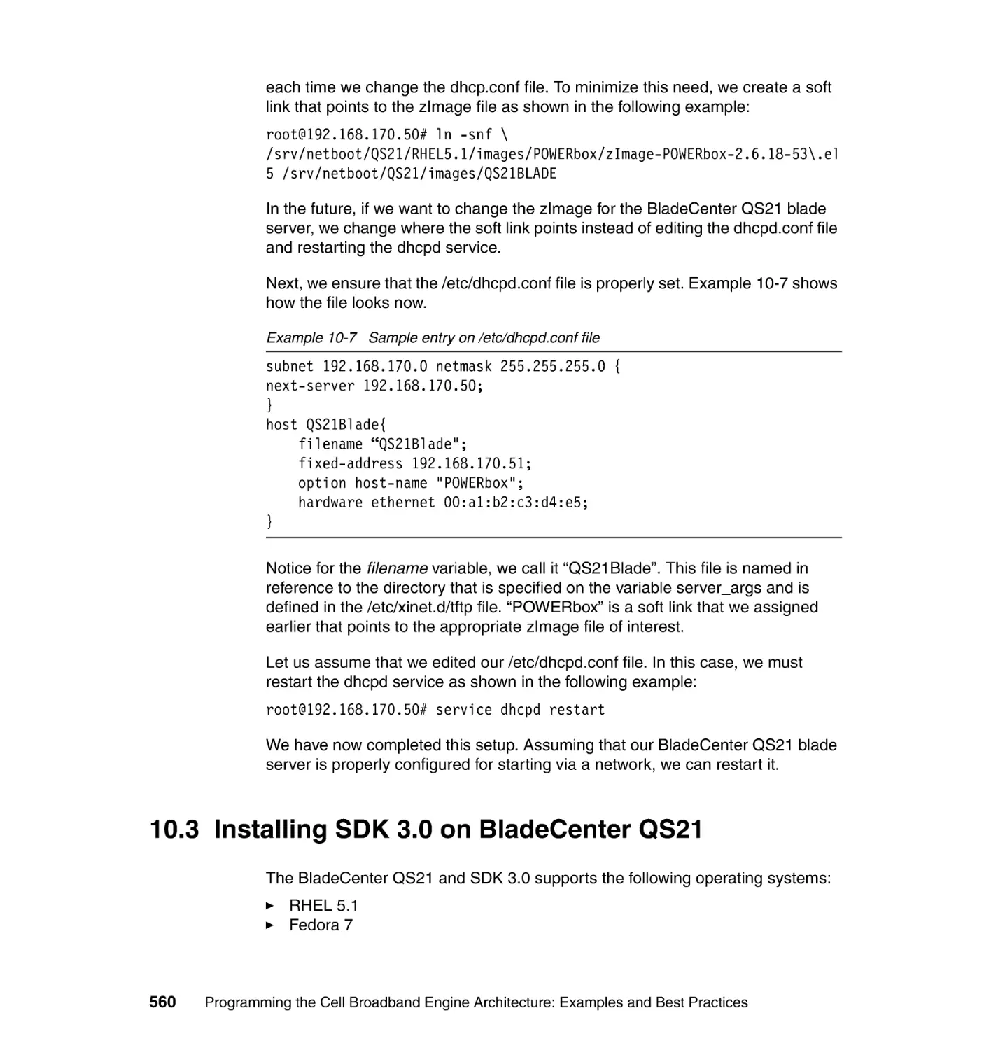
10.2.4 Example of installation from network storage . . . . . . . . . . . . . . . . 550
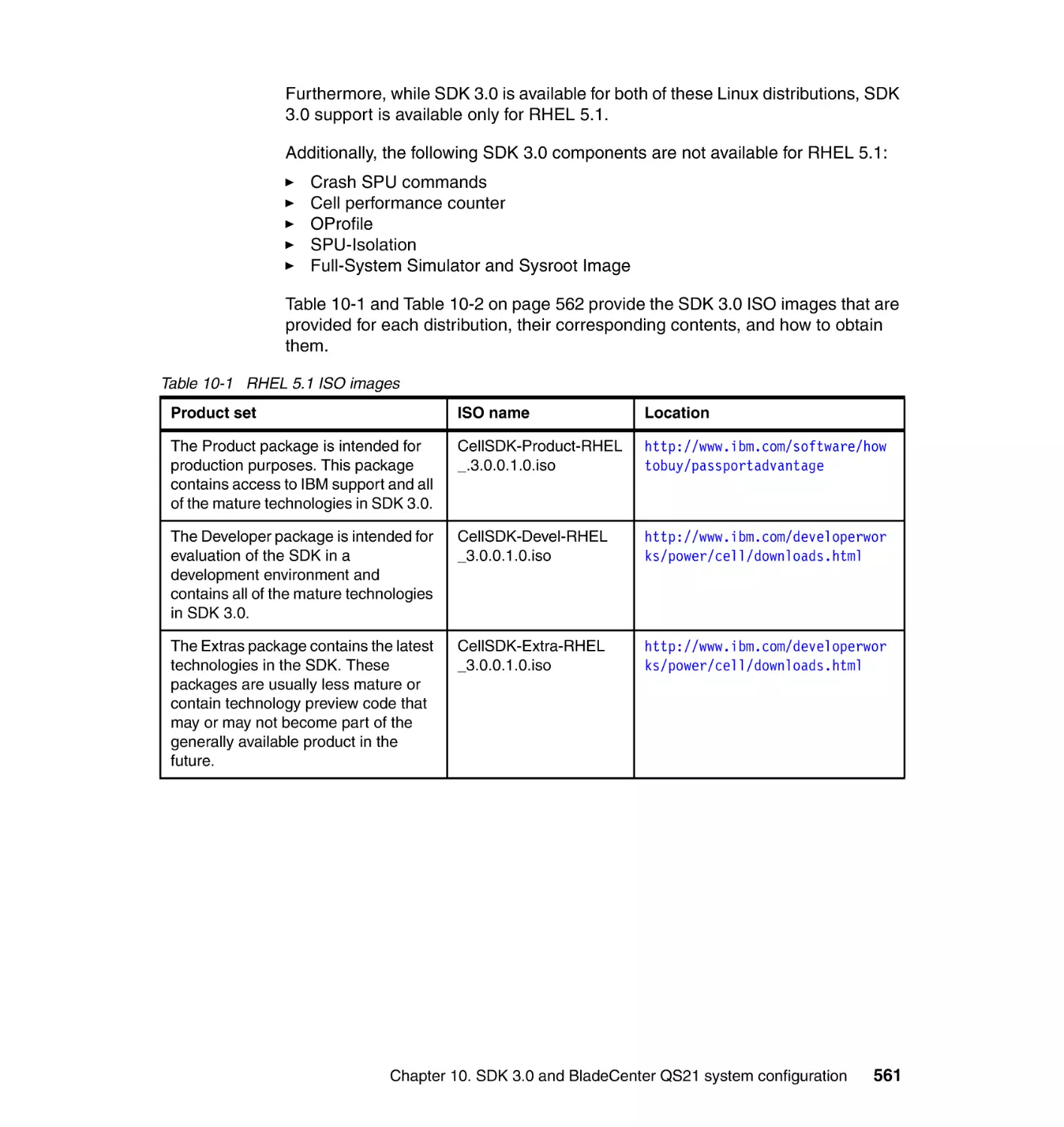
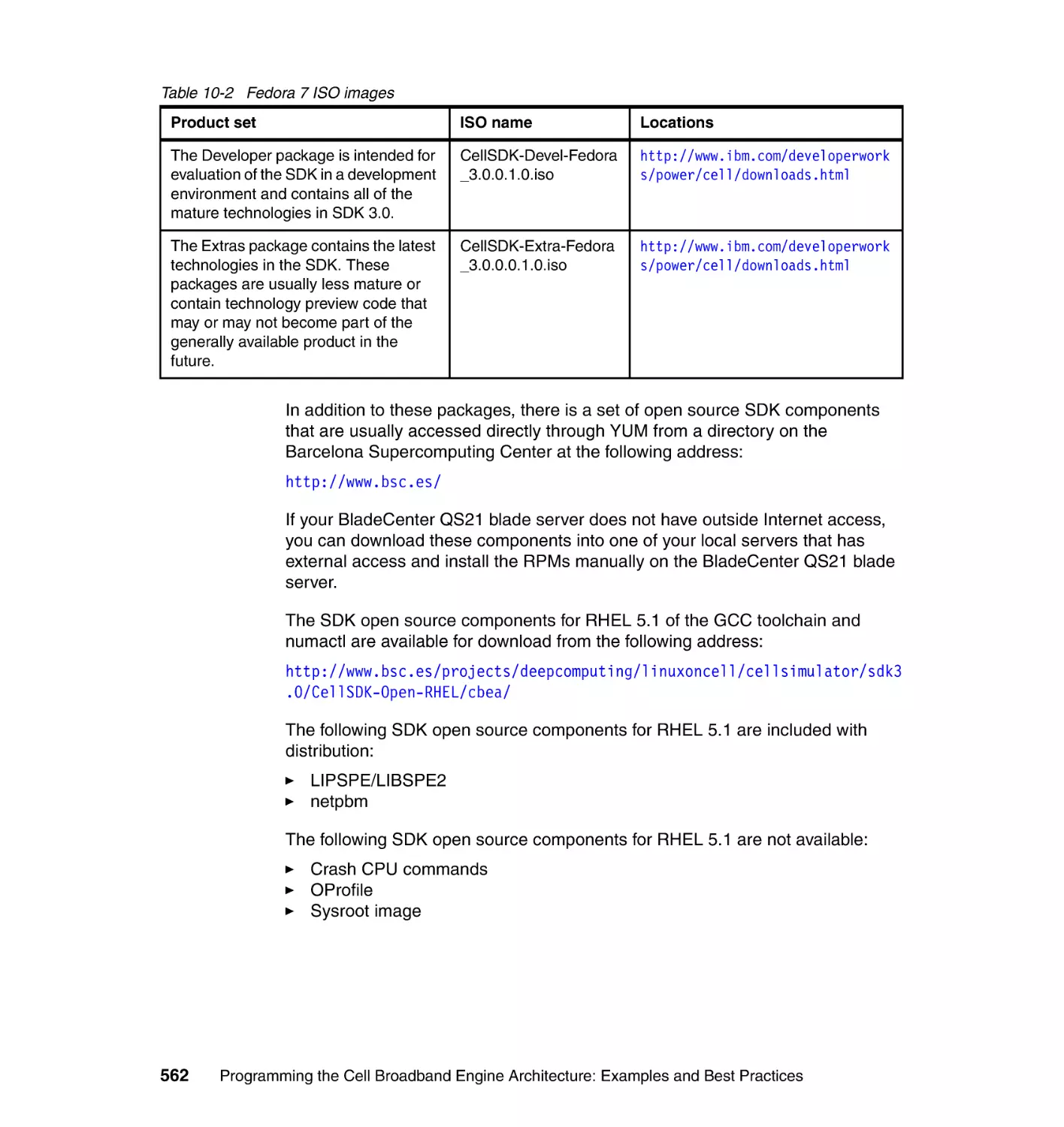
10.3 Installing SDK 3.0 on BladeCenter QS21 . . . . . . . . . . . . . . . . . . . . . . . 560
10.3.1 Pre-installation steps . . . . . . . . . . . . . . . . . . . . . . . . . . . . . . . . . . . 563
10.3.2 Installation steps . . . . . . . . . . . . . . . . . . . . . . . . . . . . . . . . . . . . . . 564
10.3.3 Post-installation steps . . . . . . . . . . . . . . . . . . . . . . . . . . . . . . . . . . 564
viii
Programming the Cell Broadband Engine Architecture: Examples and Best Practices
10.4 Firmware considerations . . . . . . . . . . . . . . . . . . . . . . . . . . . . . . . . . . . . 565
10.4.1 Updating firmware for the BladeCenter QS21. . . . . . . . . . . . . . . . 566
10.5 Options for managing multiple blades . . . . . . . . . . . . . . . . . . . . . . . . . . 569
10.5.1 Distributed Image Management . . . . . . . . . . . . . . . . . . . . . . . . . . 569
10.5.2 Extreme Cluster Administration Toolkit . . . . . . . . . . . . . . . . . . . . . 589
10.6 Method for installing a minimized distribution . . . . . . . . . . . . . . . . . . . . 593
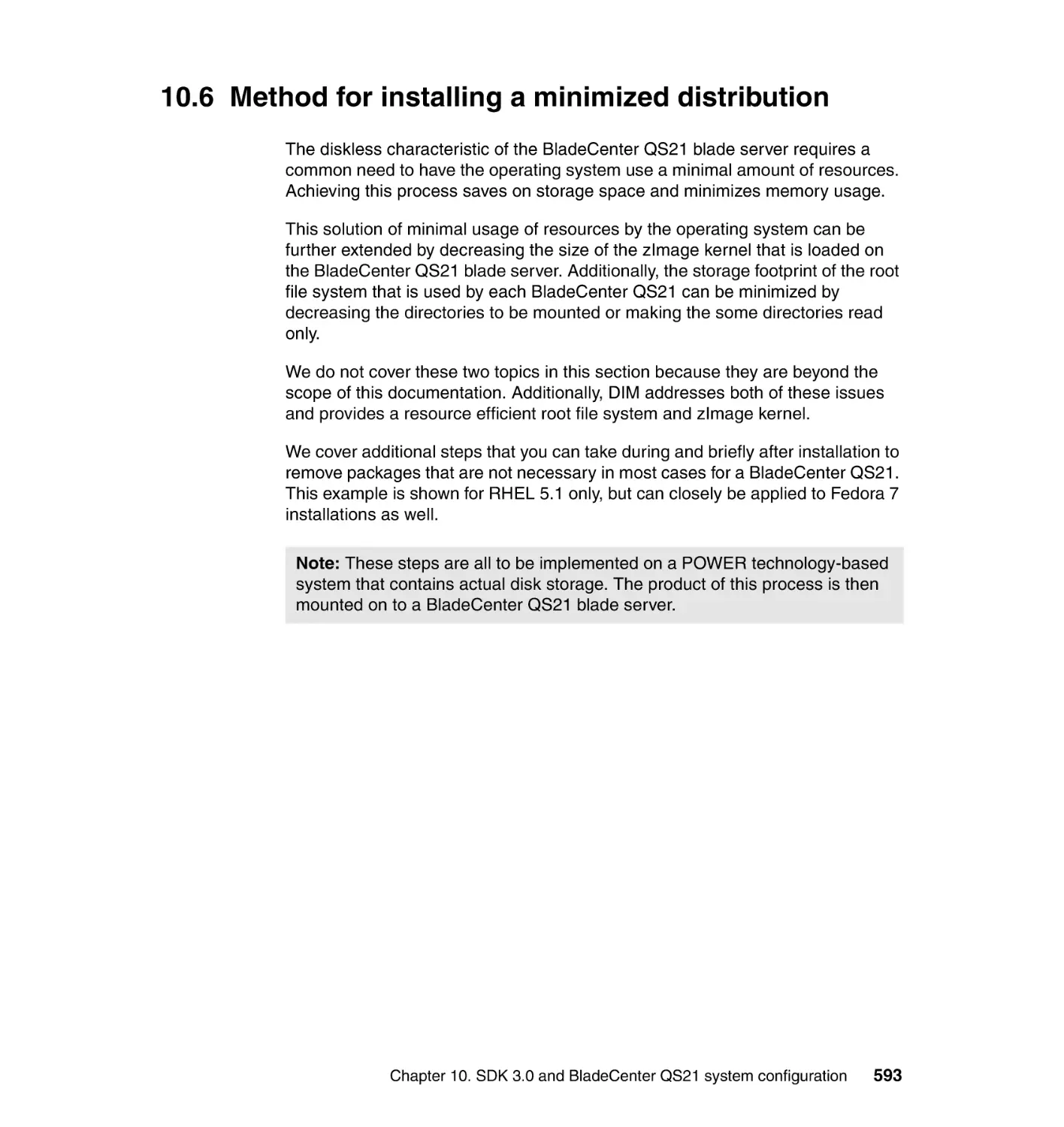
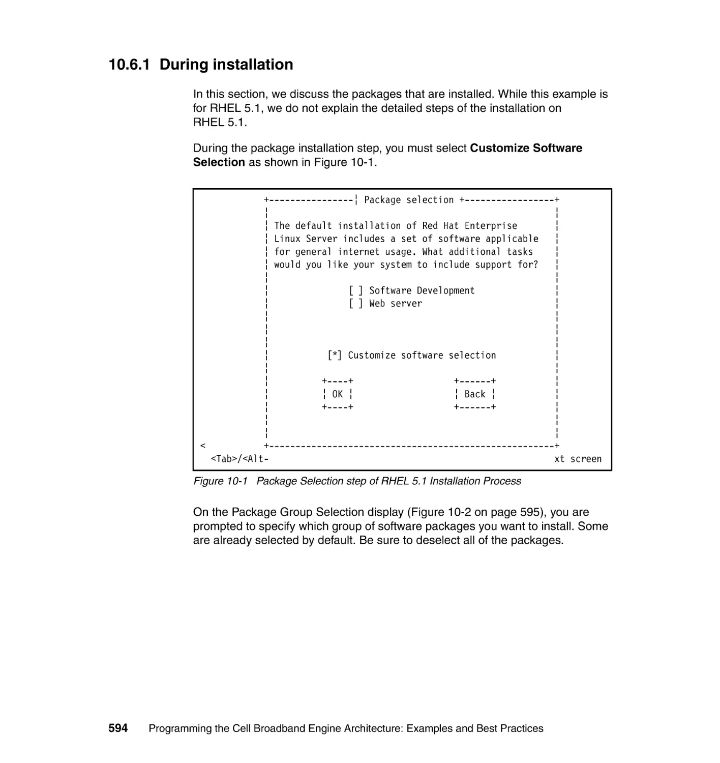
10.6.1 During installation . . . . . . . . . . . . . . . . . . . . . . . . . . . . . . . . . . . . . 594
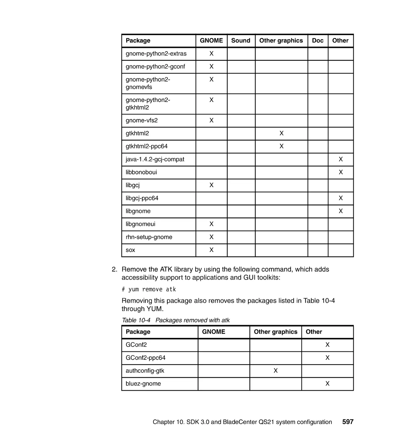
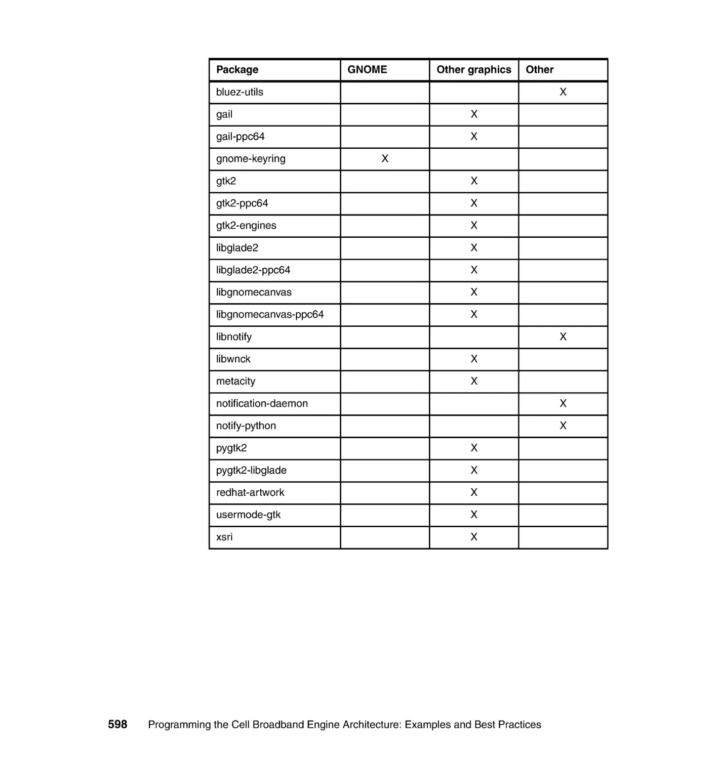
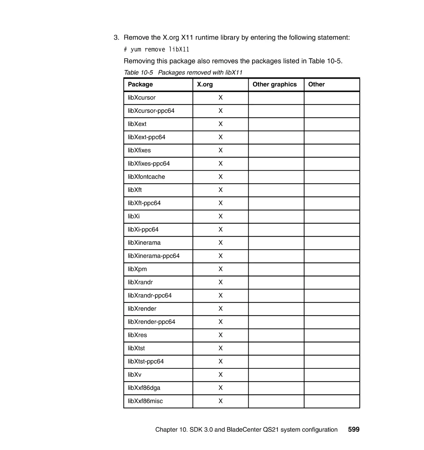
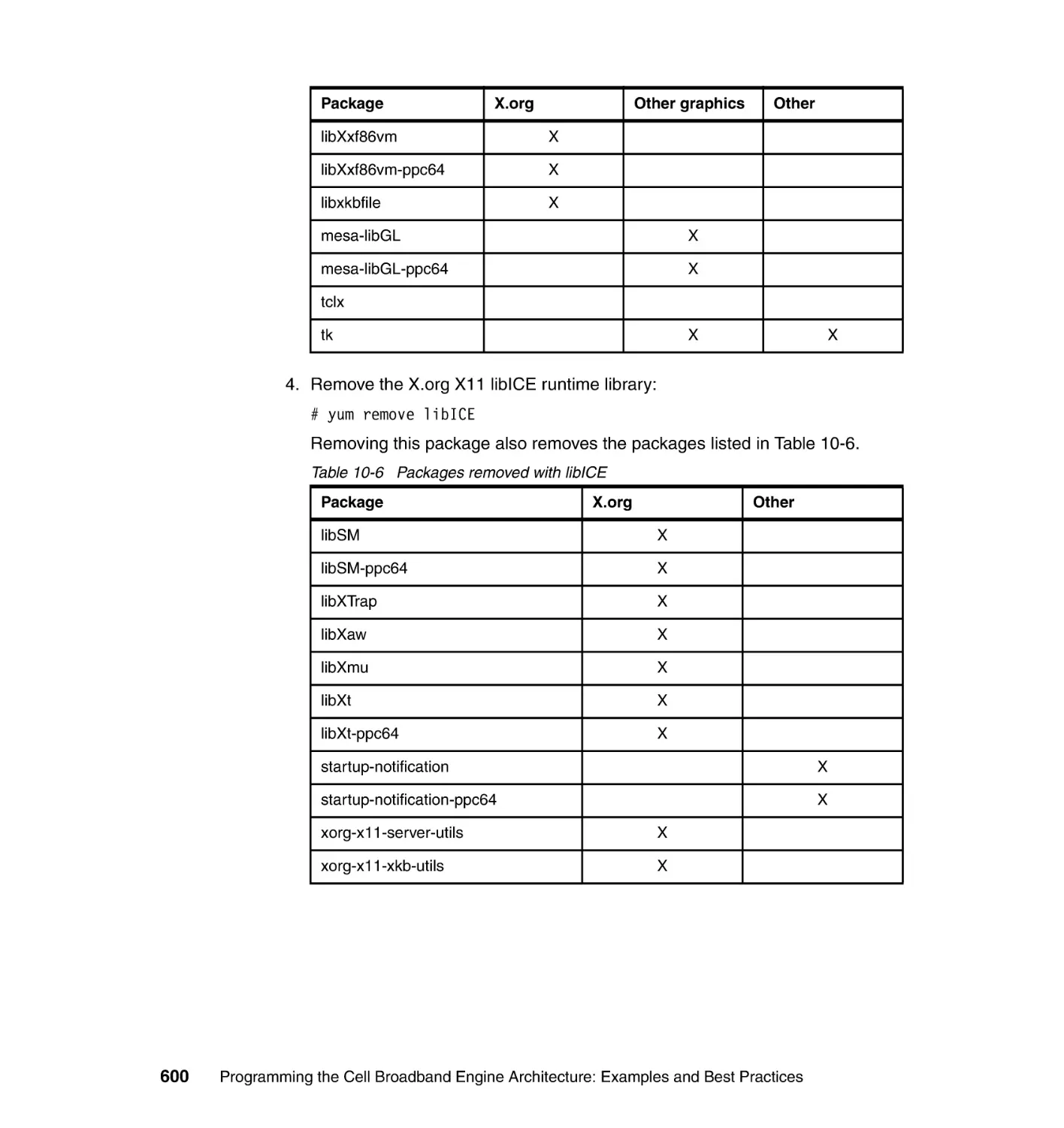
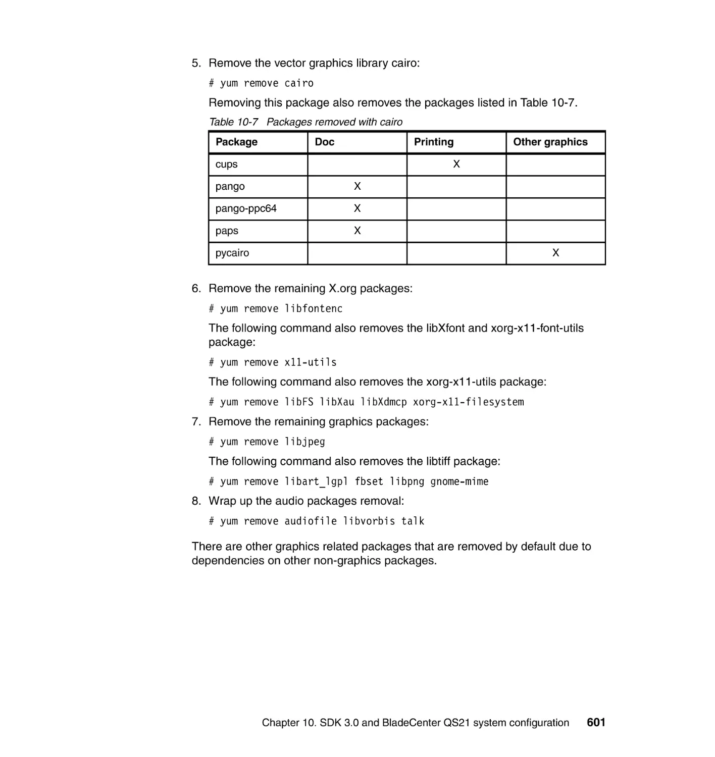
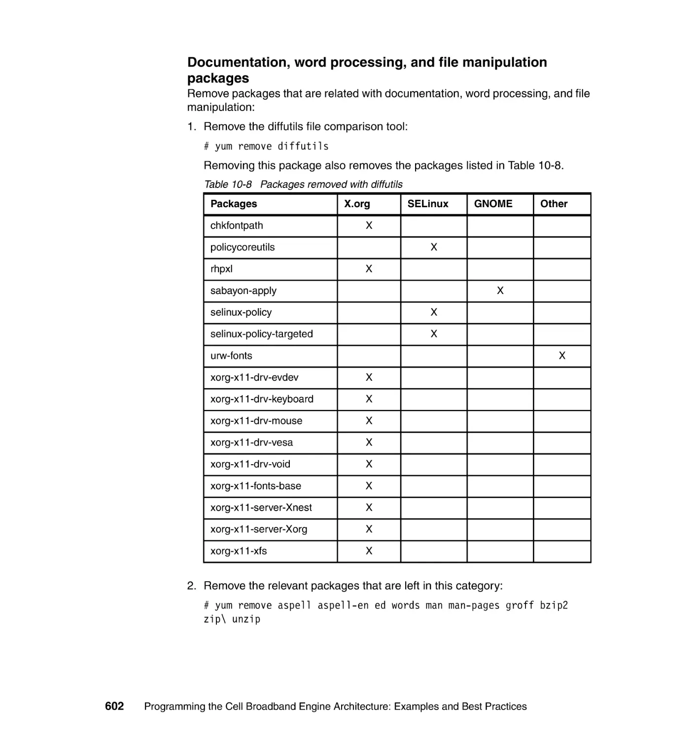
10.6.2 Post-installation package removal . . . . . . . . . . . . . . . . . . . . . . . . 596
10.6.3 Shutting off services . . . . . . . . . . . . . . . . . . . . . . . . . . . . . . . . . . . 604
Part 5. Appendixes . . . . . . . . . . . . . . . . . . . . . . . . . . . . . . . . . . . . . . . . . . . . . . . . . . . . . . . . 605
Appendix A. Software Developer Kit 3.0 topic index . . . . . . . . . . . . . . . . 607
Appendix B. Additional material . . . . . . . . . . . . . . . . . . . . . . . . . . . . . . . . 615
Locating the Web material . . . . . . . . . . . . . . . . . . . . . . . . . . . . . . . . . . . . . . . 615
Using the Web material . . . . . . . . . . . . . . . . . . . . . . . . . . . . . . . . . . . . . . . . . 616
How to use the Web material . . . . . . . . . . . . . . . . . . . . . . . . . . . . . . . . . . 616
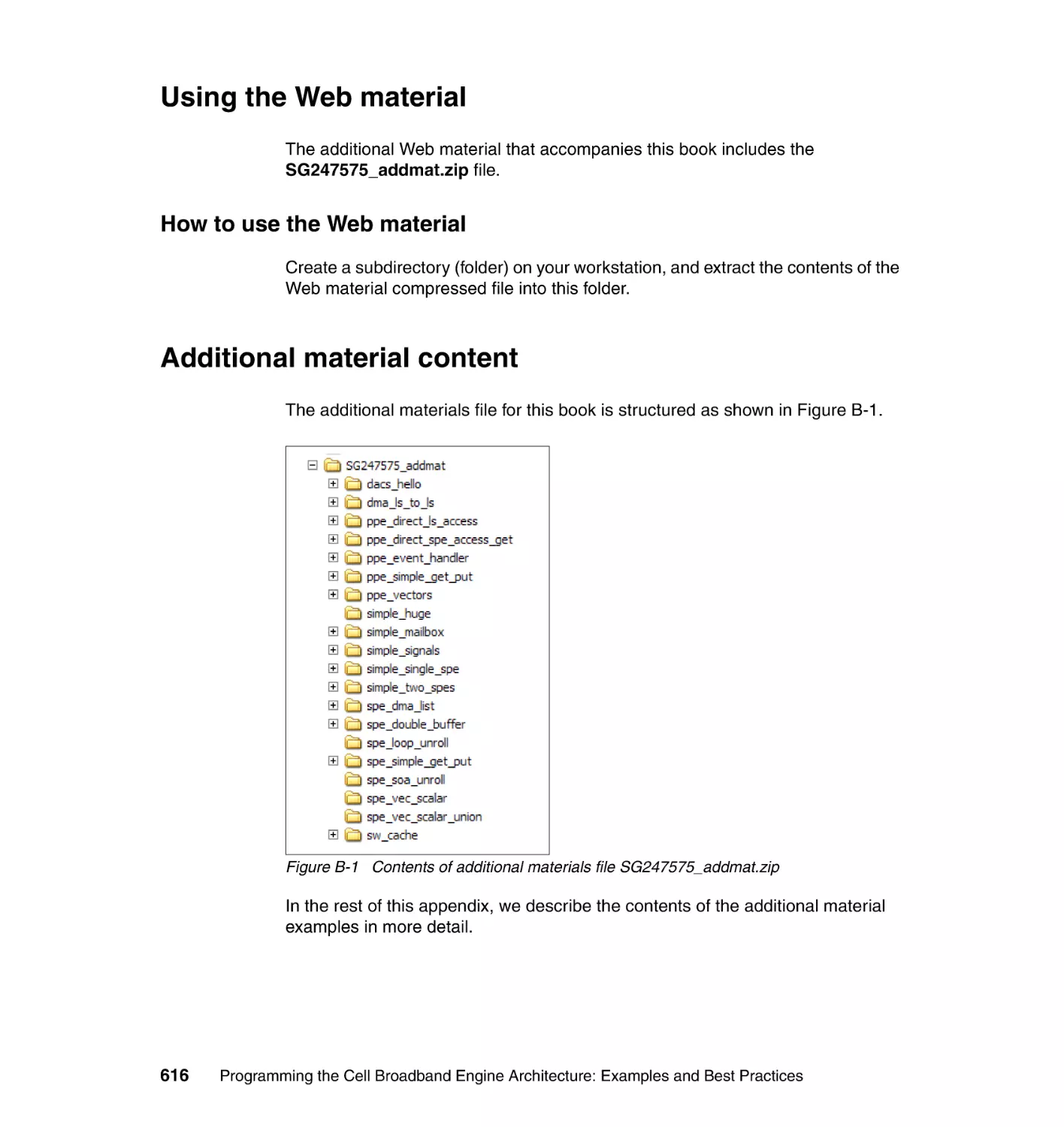
Additional material content . . . . . . . . . . . . . . . . . . . . . . . . . . . . . . . . . . . . . . . 616
Data Communication and Synchronization programming example . . . . . . . . 617
DaCS synthetic example . . . . . . . . . . . . . . . . . . . . . . . . . . . . . . . . . . . . . . 617
Task parallelism and PPE programming examples . . . . . . . . . . . . . . . . . . . . 617
Simple PPU vector/SIMD code . . . . . . . . . . . . . . . . . . . . . . . . . . . . . . . . . 617
Running a single SPE . . . . . . . . . . . . . . . . . . . . . . . . . . . . . . . . . . . . . . . . 618
Running multiple SPEs concurrently . . . . . . . . . . . . . . . . . . . . . . . . . . . . . 618
Data transfer examples . . . . . . . . . . . . . . . . . . . . . . . . . . . . . . . . . . . . . . . . . 618
Direct SPE access ‘get’ example . . . . . . . . . . . . . . . . . . . . . . . . . . . . . . . 618
SPU initiated basic DMA between LS and main storage . . . . . . . . . . . . . 618
SPU initiated DMA list transfers between LS and main storage . . . . . . . . 619
PPU initiated DMA transfers between LS and main storage. . . . . . . . . . . 619
Direct PPE access to LS of some SPEs . . . . . . . . . . . . . . . . . . . . . . . . . . 619
Multistage pipeline using LS-to-LS DMA transfer . . . . . . . . . . . . . . . . . . . 619
SPU software managed cache . . . . . . . . . . . . . . . . . . . . . . . . . . . . . . . . . 620
Double buffering . . . . . . . . . . . . . . . . . . . . . . . . . . . . . . . . . . . . . . . . . . . . 620
Huge pages. . . . . . . . . . . . . . . . . . . . . . . . . . . . . . . . . . . . . . . . . . . . . . . . 620
Inter-processor communication examples . . . . . . . . . . . . . . . . . . . . . . . . . . . 620
Simple mailbox . . . . . . . . . . . . . . . . . . . . . . . . . . . . . . . . . . . . . . . . . . . . . 620
Simple signals . . . . . . . . . . . . . . . . . . . . . . . . . . . . . . . . . . . . . . . . . . . . . . 621
PPE event handler . . . . . . . . . . . . . . . . . . . . . . . . . . . . . . . . . . . . . . . . . . 621
SPU programming examples . . . . . . . . . . . . . . . . . . . . . . . . . . . . . . . . . . . . . 621
SPE loop unrolling. . . . . . . . . . . . . . . . . . . . . . . . . . . . . . . . . . . . . . . . . . . 621
SPE SOA loop unrolling . . . . . . . . . . . . . . . . . . . . . . . . . . . . . . . . . . . . . . 621
SPE scalar-to-vector conversion using insert and extract intrinsics . . . . . 622
SPE scalar-to-vector conversion using unions . . . . . . . . . . . . . . . . . . . . . 622
Contents
ix
Related publications . . . . . . . . . . . . . . . . . . . . . . . . . . . . . . . . . . . . . . . . . . 623
IBM Redbooks . . . . . . . . . . . . . . . . . . . . . . . . . . . . . . . . . . . . . . . . . . . . . . . . 623
Other publications . . . . . . . . . . . . . . . . . . . . . . . . . . . . . . . . . . . . . . . . . . . . . 623
Online resources . . . . . . . . . . . . . . . . . . . . . . . . . . . . . . . . . . . . . . . . . . . . . . 625
How to get Redbooks . . . . . . . . . . . . . . . . . . . . . . . . . . . . . . . . . . . . . . . . . . . 626
Help from IBM . . . . . . . . . . . . . . . . . . . . . . . . . . . . . . . . . . . . . . . . . . . . . . . . 626
Index . . . . . . . . . . . . . . . . . . . . . . . . . . . . . . . . . . . . . . . . . . . . . . . . . . . . . . . 627
x
Programming the Cell Broadband Engine Architecture: Examples and Best Practices
Notices
This information was developed for products and services offered in the U.S.A.
IBM may not offer the products, services, or features discussed in this document in other countries. Consult
your local IBM representative for information on the products and services currently available in your area.
Any reference to an IBM product, program, or service is not intended to state or imply that only that IBM
product, program, or service may be used. Any functionally equivalent product, program, or service that
does not infringe any IBM intellectual property right may be used instead. However, it is the user's
responsibility to evaluate and verify the operation of any non-IBM product, program, or service.
IBM may have patents or pending patent applications covering subject matter described in this document.
The furnishing of this document does not give you any license to these patents. You can send license
inquiries, in writing, to:
IBM Director of Licensing, IBM Corporation, North Castle Drive, Armonk, NY 10504-1785 U.S.A.
The following paragraph does not apply to the United Kingdom or any other country where such
provisions are inconsistent with local law: INTERNATIONAL BUSINESS MACHINES CORPORATION
PROVIDES THIS PUBLICATION "AS IS" WITHOUT WARRANTY OF ANY KIND, EITHER EXPRESS OR
IMPLIED, INCLUDING, BUT NOT LIMITED TO, THE IMPLIED WARRANTIES OF NON-INFRINGEMENT,
MERCHANTABILITY OR FITNESS FOR A PARTICULAR PURPOSE. Some states do not allow disclaimer
of express or implied warranties in certain transactions, therefore, this statement may not apply to you.
This information could include technical inaccuracies or typographical errors. Changes are periodically made
to the information herein; these changes will be incorporated in new editions of the publication. IBM may
make improvements and/or changes in the product(s) and/or the program(s) described in this publication at
any time without notice.
Any references in this information to non-IBM Web sites are provided for convenience only and do not in any
manner serve as an endorsement of those Web sites. The materials at those Web sites are not part of the
materials for this IBM product and use of those Web sites is at your own risk.
IBM may use or distribute any of the information you supply in any way it believes appropriate without
incurring any obligation to you.
Information concerning non-IBM products was obtained from the suppliers of those products, their published
announcements or other publicly available sources. IBM has not tested those products and cannot confirm
the accuracy of performance, compatibility or any other claims related to non-IBM products. Questions on
the capabilities of non-IBM products should be addressed to the suppliers of those products.
This information contains examples of data and reports used in daily business operations. To illustrate them
as completely as possible, the examples include the names of individuals, companies, brands, and products.
All of these names are fictitious and any similarity to the names and addresses used by an actual business
enterprise is entirely coincidental.
COPYRIGHT LICENSE:
This information contains sample application programs in source language, which illustrate programming
techniques on various operating platforms. You may copy, modify, and distribute these sample programs in
any form without payment to IBM, for the purposes of developing, using, marketing or distributing application
programs conforming to the application programming interface for the operating platform for which the
sample programs are written. These examples have not been thoroughly tested under all conditions. IBM,
therefore, cannot guarantee or imply reliability, serviceability, or function of these programs.
© Copyright IBM Corp. 2008. All rights reserved.
xi
Trademarks
IBM, the IBM logo, and ibm.com are trademarks or registered trademarks of International Business
Machines Corporation in the United States, other countries, or both. These and other IBM trademarked
terms are marked on their first occurrence in this information with the appropriate symbol (® or ™),
indicating US registered or common law trademarks owned by IBM at the time this information was
published. Such trademarks may also be registered or common law trademarks in other countries. A current
list of IBM trademarks is available on the Web at http://www.ibm.com/legal/copytrade.shtml
AIX 5L™
AIX®
alphaWorks®
BladeCenter®
Blue Gene®
IBM®
POWER™
PowerPC Architecture™
PowerPC®
Redbooks®
Redbooks (logo)
System i™
System p™
System x™
®
The following terms are trademarks of other companies:
AMD, AMD Opteron, the AMD Arrow logo, and combinations thereof, are trademarks of Advanced Micro
Devices, Inc.
InfiniBand, and the InfiniBand design marks are trademarks and/or service marks of the InfiniBand Trade
Association.
Snapshot, and the NetApp logo are trademarks or registered trademarks of NetApp, Inc. in the U.S. and
other countries.
SUSE, the Novell logo, and the N logo are registered trademarks of Novell, Inc. in the United States and
other countries.
Cell Broadband Engine and Cell/B.E. are trademarks of Sony Computer Entertainment, Inc., in the United
States, other countries, or both and is used under license therefrom.
Java, and all Java-based trademarks are trademarks of Sun Microsystems, Inc. in the United States, other
countries, or both.
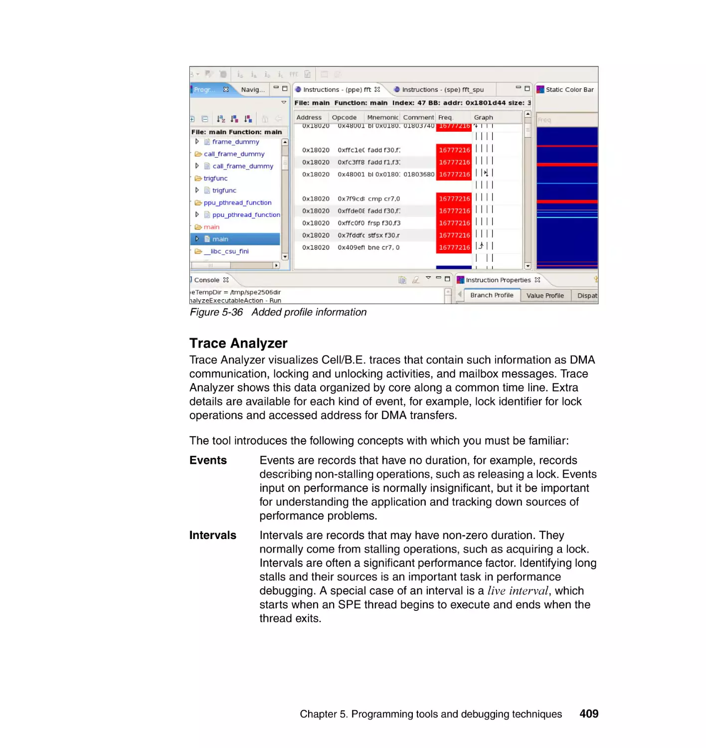
ESP, Excel, Fluent, Microsoft, Visual Basic, Visual C++, Windows, and the Windows logo are trademarks of
Microsoft Corporation in the United States, other countries, or both.
Intel, Intel logo, Intel Inside logo, and Intel Centrino logo are trademarks or registered trademarks of Intel
Corporation or its subsidiaries in the United States, other countries, or both.
Linux is a trademark of Linus Torvalds in the United States, other countries, or both.
MultiCore Plus is a trademark of Mercury Computer Systems, Inc. in the United States, other countries, or
both.
Other company, product, or service names may be trademarks or service marks of others.
xii
Programming the Cell Broadband Engine Architecture: Examples and Best Practices
Preface
In this IBM® Redbooks® publication, we provide an introduction to the Cell
Broadband Engine™ (Cell/B.E.™) platform. We show detailed samples from
real-world application development projects and provide tips and best practices
for programming Cell/B.E. applications.
We also describe the content and packaging of the IBM Software Development
Kit (SDK) version 3.0 for Multicore Acceleration. This SDK provides all the tools
and resources that are necessary to build applications that run IBM
BladeCenter® QS21 and QS20 blade servers. We show in-depth and real-world
usage of the tools and resources found in the SDK. We also provide installation,
configuration, and administration tips and best practices for the IBM BladeCenter
QS21. In addition, we discuss the supporting software that is provided by IBM
alphaWorks®.
This book was written for developers and programmers, IBM technical
specialists, Business Partners, Clients, and the Cell/B.E. community to
understand how to develop applications by using the Cell/B.E. SDK 3.0.
The team that wrote this book
This book was produced by a team of specialists from around the world working
at the International Technical Support Organization (ITSO), Austin Center.
Abraham Arevalo is a Software Engineer in the Linux® Technology Center’s
Test Department in Austin, Texas. He has worked on ensuring quality and
functional performance of Red Hat Enterprise Linux (RHEL) 5.1 and Fedora 7
distributions on BladeCenter QS20 and QS21 blade servers. Additionally,
Abraham has been involved on other Cell/B.E.-related projects including
expanding its presence on consumer electronics. He has prior experience
working with hardware development mostly with System on Chip design.
Ricardo M. Matinata is an Advisory Software Engineer for the Linux Technology
Center, in IBM Systems and Technology Group at IBM Brazil. He has over 10
years of experience in software research and development. He has been part of
the global Cell/B.E. SDK development team, in the Toolchain (integrated
development environment (IDE)) area, for almost two years. Ricardo’s areas of
expertise include system software and application development for product and
© Copyright IBM Corp. 2008. All rights reserved.
xiii
open source types of projects, Linux, programming models, development tools,
debugging, and networking.
Maharaja (Raj) Pandian is a High Performance Computing specialist working on
scientific applications in the IBM Worldwide Advanced Client Technology (A.C.T!)
Center, Poughkeepsie, NY. Currently, he is developing and benchmarking
Financial Sector Services applications on the Cell/B.E. He has twenty years of
experience in high performance computing, software development, and market
support. His areas of expertise include parallel algorithms for distributed memory
system and symmetric multiprocessor system, numerical methods for partial
differential equations, performance optimization, and benchmarking. Maharaja
has worked with engineering analysis ISV applications, such as MSC/NASTRAN
(Finite Element Analysis) and Fluent™ (Computational Fluid Dynamics), for
several years. He has also worked with weather modeling applications on IBM
AIX® and Linux clusters. He holds a Ph.D. in Applied Mathematics from the
University of Texas, Arlington.
Eitan Peri works in the IBM Haifa Research Lab as the technical lead for
Cell/B.E. pre-sales activities in Israel. He is currently working on projects
focusing on porting applications to the CBEA within the health care, computer
graphics, aerospace, and defense industries. He has nine years of experience in
real-time programming, chip design, and chip verification. His areas of expertise
include Cell/B.E. programming and consulting, application parallelization and
optimization, algorithm performance analysis, and medical imaging. Eitan holds
a Bachelor of Science degree in Computer Engineering from the Israel Institute
of Technology (the Technion) and a Master of Science degree in Biomedical
Engineering from Tel-Aviv University, where he specialized in brain imaging
analysis.
Kurtis Ruby is a software consultant with IBM Lab Services at IBM in Rochester,
Minnesota. He has over twenty-five years of experience in various programming
assignments in IBM. His expertise includes Cell/B.E. programming and
consulting. Kurtis holds a degree in mathematics from Iowa State University.
Francois Thomas is an IBM Certified IT Specialist working on high-performance
computing (HPC) pre-sales in the Deep Computing Europe organization in
France. He has 18 years of experience in the field of scientific and technical
computing. His areas of expertise include application code tuning and
parallelization as well as Linux clusters management. He works with weather
forecast institutions in Europe on enabling petroleum engineering ISV
applications to the Linux on Power platform. Francois holds a PhD. in Physics
from ENSAM/Paris VI University.
xiv
Programming the Cell Broadband Engine Architecture: Examples and Best Practices
Chris Almond is an ITSO Project Leader and IT Architect based at the ITSO
Center in Austin, Texas. In his current role, he specializes in managing content
development projects focused on Linux, AIX 5L™ systems engineering, and
other innovation programs. He has a total of 17 years of IT industry experience,
including the last eight with IBM. Chris handled the production of this IBM
Redbooks publication.
Acknowledgements
This IBM Redbooks publication would not have been possible without the
generous support and contributions provided many from IBM. The authoring
team gratefully acknowledges the critical support and sponsorship for this project
provided by the following IBM specialists:
Rebecca Austen, Director, Systems Software, Systems and Technology
Group
Daniel Brokenshire, Senior Technical Staff Member and Software Architect,
Quasar/Cell Broadband Engine Software Development, Systems and
Technology Group
Paula Richards, Director, Global Engineering Solutions, Systems and
Technology Group
Jeffrey Scheel, Blue Gene® Software Program Manager and Software
Architect, Systems and Technology Group
Tanaz Sowdagar, Marketing Manager, Systems and Technology Group
We also thank the following IBM specialists for their significant input to this
project during the development and technical review process:
Marina Biberstein, Research Scientist, Haifa Research Lab, IBM Research
Michael Brutman, Solutions Architect, Lab Services, IBM Systems and
Technology Group
Dean Burdick, Developer, Cell Software Development, IBM Systems and
Technology Group
Catherine Crawford, Senior Technical Staff Member and Chief Architect, Next
Generation Systems Software, IBM Systems and Technology Group
Bruce D’Amora, Research Scientist, Systems Engineering, IBM Research
Matthew Drahzal, Software Architect, Deep Computing, IBM Systems and
Technology Group
Matthias Fritsch, Enterprise System Development, IBM Systems and
Technology Group
Preface
xv
Gad Haber, Manager, Performance Analysis and Optimization Technology,
Haifa Reseach Lab, IBM Research
Francesco Iorio, Solutions Architect, Next Generation Computing, IBM
Software Group
Kirk Jordan, Solutions Executive, Deep Computing and Emerging HPC
Technologies, IBM Systems and Technology Group
Melvin Kendrick, Manager, Cell Ecosystem Technical Enablement, IBM
Systems and Technology Group
Mark Mendell, Team Lead, Cell/B.E. Compiler Development, IBM Software
Group
Michael P. Perrone, Ph.D., Manager Cell Solutions, IBM Systems and
Technology Group
Juan Jose Porta, Executive Architect HPC and e-Science Platforms, IBM
Systems and Technology Group
Uzi Shvadron, Research Scientist, Cell/B.E. Performance Tools, Haifa
Research Lab, IBM Research
Van To, Advisory Software Engineer, Cell/B.E. and Next Generation
Computing Systems, IBM Systems and Technology Group
Duc J. Vianney, Ph. D, Technical Education Lead, Cell/B.E. Ecosystem and
Solutions Enablement, IBM Systems and Technology Group
Brian Watt, Systems Development, Quasar Design Center Development, IBM
Systems and Technology Group
Ulrich Weigand, Developer, Linux on Cell/B.E., IBM Systems and Technology
Group
Cornell Wright, Developer, Cell Software Development, IBM Systems and
Technology Group
xvi
Programming the Cell Broadband Engine Architecture: Examples and Best Practices
Become a published author
Join us for a two- to six-week residency program! Help write a book dealing with
specific products or solutions, while getting hands-on experience with
leading-edge technologies. You will have the opportunity to team with IBM
technical professionals, Business Partners, and Clients.
Your efforts will help increase product acceptance and customer satisfaction. As
a bonus, you will develop a network of contacts in IBM development labs, and
increase your productivity and marketability.
Find out more about the residency program, browse the residency index, and
apply online at:
ibm.com/redbooks/residencies.html
Comments welcome
Your comments are important to us!
We want our books to be as helpful as possible. Send us your comments about
this book or other IBM Redbooks in one of the following ways:
Use the online Contact us review Redbooks form found at:
ibm.com/redbooks
Send your comments in an e-mail to:
redbooks@us.ibm.com
Mail your comments to:
IBM Corporation, International Technical Support Organization
Dept. HYTD Mail Station P099
2455 South Road
Poughkeepsie, NY 12601-5400
Preface
xvii
xviii
Programming the Cell Broadband Engine Architecture: Examples and Best Practices
Part 1
Part
1
Introduction to the
Cell Broadband
Engine Architecture
The Cell Broadband Engine (Cell/B.E.) Architecture (CBEA) is a new class of
multicore processors being brought to the consumer and business market. It has
a radically different design than those offered by other consumer and business
chip makers in the global market. This radical departure warrants a brief
discussion of the Cell/B.E. hardware and software architecture.
There is also a brief discussion of the IBM Software Development Kit (SDK) for
Multicore Acceleration from a content and packaging perspective. These
discussions complement the in-depth content of the remaining chapters of this
book.
Specifically, this part includes the following chapters:
Chapter 1, “Cell Broadband Engine overview” on page 3
Chapter 2, “IBM SDK for Multicore Acceleration” on page 17
© Copyright IBM Corp. 2008. All rights reserved.
1
2
Programming the Cell Broadband Engine Architecture: Examples and Best Practices
1
Chapter 1.
Cell Broadband Engine
overview
The Cell Broadband Engine (Cell/B.E.) processor is the first implementation of a
new multiprocessor family that conforms to the Cell/B.E. Architecture (CBEA).
The CBEA and the Cell/B.E. processor are the result of a collaboration between
Sony, Toshiba, and IBM (known as STI), which formally began in early 2001.
Although the Cell/B.E. processor is initially intended for applications in media-rich
consumer-electronics devices, such as game consoles and high-definition
televisions, the architecture has been designed to enable fundamental advances
in processor performance. These advances are expected to support a broad
range of applications in both commercial and scientific fields.
In this chapter, we discuss the following topics:
1.1, “Motivation” on page 4
1.2, “Scaling the three performance-limiting walls” on page 6
1.3, “Hardware environment” on page 8
1.4, “Programming environment” on page 11
© Copyright IBM Corp. 2008. All rights reserved.
3
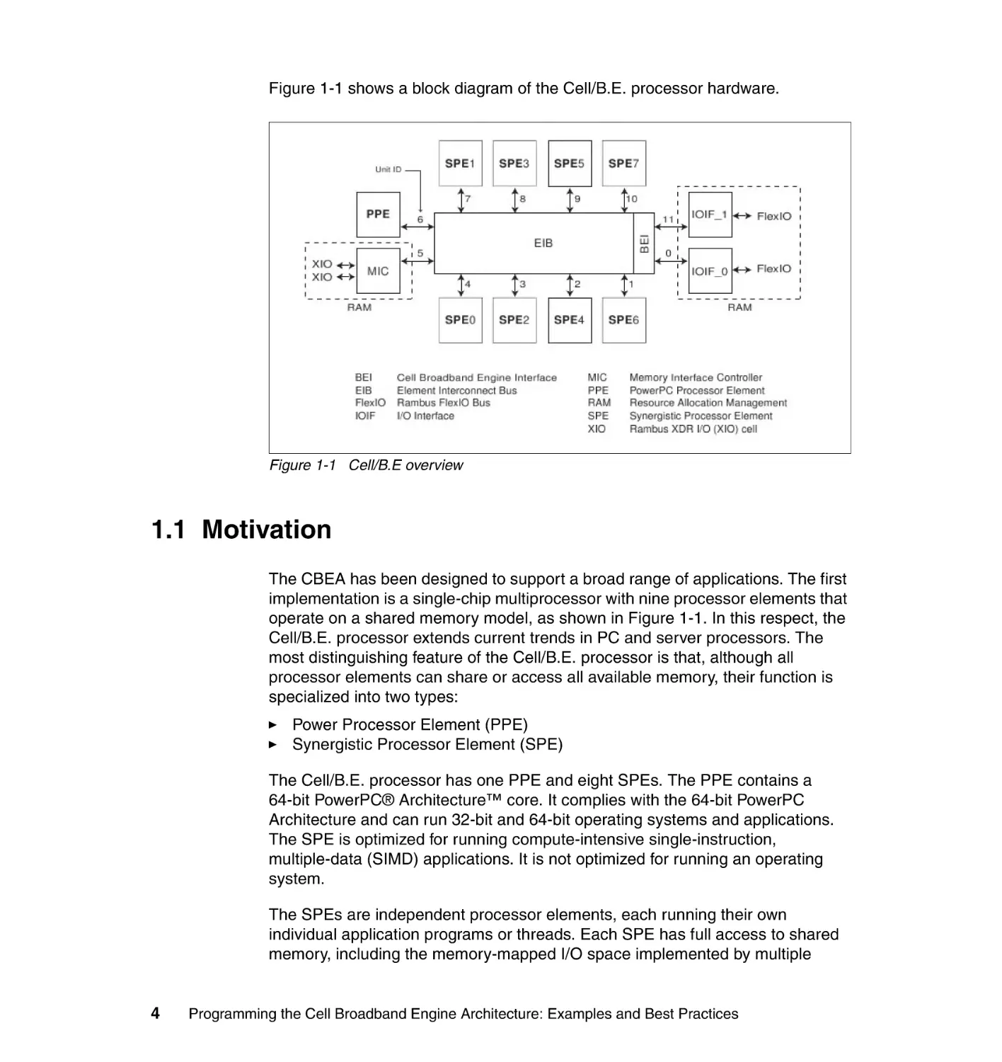
Figure 1-1 shows a block diagram of the Cell/B.E. processor hardware.
Figure 1-1 Cell/B.E overview
1.1 Motivation
The CBEA has been designed to support a broad range of applications. The first
implementation is a single-chip multiprocessor with nine processor elements that
operate on a shared memory model, as shown in Figure 1-1. In this respect, the
Cell/B.E. processor extends current trends in PC and server processors. The
most distinguishing feature of the Cell/B.E. processor is that, although all
processor elements can share or access all available memory, their function is
specialized into two types:
Power Processor Element (PPE)
Synergistic Processor Element (SPE)
The Cell/B.E. processor has one PPE and eight SPEs. The PPE contains a
64-bit PowerPC® Architecture™ core. It complies with the 64-bit PowerPC
Architecture and can run 32-bit and 64-bit operating systems and applications.
The SPE is optimized for running compute-intensive single-instruction,
multiple-data (SIMD) applications. It is not optimized for running an operating
system.
The SPEs are independent processor elements, each running their own
individual application programs or threads. Each SPE has full access to shared
memory, including the memory-mapped I/O space implemented by multiple
4
Programming the Cell Broadband Engine Architecture: Examples and Best Practices
direct memory access (DMA) units. There is a mutual dependence between the
PPE and the SPEs. The SPEs depend on the PPE to run the operating system,
and, in many cases, the top-level thread control for an application. The PPE
depends on the SPEs to provide the bulk of the application performance.
The SPEs are designed to be programmed in high-level languages, such as
C/C++. They support a rich instruction set that includes extensive SIMD
functionality. However, like conventional processors with SIMD extensions, use of
SIMD data types is preferred, not mandatory. For programming convenience, the
PPE also supports the standard PowerPC Architecture instructions and the
vector/SIMD multimedia extensions.
To an application programmer, the Cell/B.E. processor looks like a single core,
dual-threaded processor with eight additional cores each having their own local
storage. The PPE is more adept than the SPEs at control-intensive tasks and
quicker at task switching. The SPEs are more adept at compute-intensive tasks
and slower than the PPE at task switching. However, either processor element is
capable of both types of functions. This specialization is a significant factor
accounting for the order-of-magnitude improvement in peak computational
performance and chip-area and power efficiency that the Cell/B.E. processor
achieves over conventional PC processors.
The more significant difference between the SPE and PPE lies in how they
access memory. The PPE accesses main storage (the effective address space)
with load and store instructions that move data between main storage and a
private register file, the contents of which may be cached. PPE memory access
is like that of a conventional processor technology, which is found on
conventional machines.
The SPEs, in contrast, access main storage with DMA commands that move
data and instructions between main storage and a private local memory, called
local storage (LS). An instruction-fetches and load and store instructions of an
SPE access its private LS rather than shared main storage, and the LS has no
associated cache. This three-level organization of storage (register file, LS, and
main storage), with asynchronous DMA transfers between LS and main storage,
is a radical break from conventional architecture and programming models. The
organization explicitly parallelizes computation with the transfers of data and
instructions that feed computation and store the results of computation in main
storage.
One of the motivations for this radical change is that memory latency, measured
in processor cycles, has gone up several hundredfold from about the years 1980
to 2000. The result is that application performance is, in most cases, limited by
memory latency rather than peak compute capability or peak bandwidth.
Chapter 1. Cell Broadband Engine overview
5
When a sequential program on a conventional architecture performs a load
instruction that misses in the caches, program execution can come to a halt for
several hundred cycles. (Techniques such as hardware threading can attempt to
hide these stalls, but it does not help single-threaded applications.) Compared to
this penalty, the few cycles it takes to set up a DMA transfer for an SPE are a
much better trade-off, especially considering the fact that the DMA controllers of
each of the eight SPEs can have up to 16 DMA transfers in flight simultaneously.
Anticipating DMA needs efficiently can provide just-in-time delivery of data that
may reduce this stall or eliminate them entirely. Conventional processors, even
with deep and costly speculation, manage to get, at best, a handful of
independent memory accesses in flight.
One of the DMA transfer methods of the SPE supports a list, such as a
scatter-gather list, of DMA transfers that is constructed in the local storage of an
SPE. Therefore, the DMA controller of the SPE can process the list
asynchronously while the SPE operates on previously transferred data. In
several cases, this approach to accessing memory has led to application
performance exceeding that of conventional processors by almost two orders of
magnitude. This result is significantly more than you expect from the peak
performance ratio (approximately 10 times) between the Cell/B.E. processor and
conventional PC processors. The DMA transfers can be set up and controlled by
the SPE that is sourcing or receiving the data, or in some circumstances, by the
PPE or another SPE.
1.2 Scaling the three performance-limiting walls
The Cell/B.E. overcomes three important limiters of contemporary
microprocessor performance: power use, memory use, and processor frequency.
1.2.1 Scaling the power-limitation wall
Increasingly, microprocessor performance is limited by achievable power
dissipation rather than by the number of available integrated-circuit resources
(transistors and wires). Therefore, the only way to significantly increase the
performance of microprocessors is to improve power efficiency at about the
same rate as the performance increase.
One way to increase power efficiency is to differentiate between the following
types of processors:
Processors that are optimized to run an operating system and
control-intensive code
Processors that are optimized to run compute-intensive applications
6
Programming the Cell Broadband Engine Architecture: Examples and Best Practices
The Cell/B.E. processor does this by providing a general-purpose PPE to run the
operating system and other control-plane code, as well as eight SPEs
specialized for computing data-rich (data-plane) applications. The specialized
SPEs are more compute efficient because they have simpler hardware
implementations. The hardware does not devote transistors to branch prediction,
out-of-order execution, speculative execution, shadow registers and register
renaming, extensive pipeline interlocks, and so on. By weight, more of the
transistors are used for computation than in conventional processor cores.
1.2.2 Scaling the memory-limitation wall
On multi-gigahertz symmetric multiprocessors (SMPs), even those with
integrated memory controllers, latency to DRAM memory is currently
approaching 1,000 cycles. As a result, program performance is dominated by the
activity of moving data between main storage (the effective-address space that
includes main memory) and the processor. Increasingly, compilers and even
application writers must manage this movement of data explicitly, even though
the hardware cache mechanisms are supposed to relieve them of this task.
The SPEs of the Cell/B.E. processor use two mechanisms to deal with long
main-memory latencies:
Three-level memory structure (main storage, local storage in each SPE, and
large register files in each SPE)
Asynchronous DMA transfers between main storage and local storage
These features allow programmers to schedule simultaneous data and code
transfers to cover long latencies effectively. Because of this organization, the
Cell/B.E. processor can usefully support 128 simultaneous transfers between the
eight SPE local storage and main storage. This surpasses the number of
simultaneous transfers on conventional processors by a factor of almost twenty.
1.2.3 Scaling the frequency-limitation wall
Conventional processors require increasingly deeper instruction pipelines to
achieve higher operating frequencies. This technique has reached a point of
diminishing returns, and even negative returns if power is taken into account.
By specializing the PPE and the SPEs for control and compute-intensive tasks,
respectively, the CBEA, on which the Cell/B.E. processor is based, allows both
the PPE and the SPEs to be designed for high frequency without excessive
overhead. The PPE achieves efficiency primarily by executing two threads
simultaneously rather than by optimizing single-thread performance.
Chapter 1. Cell Broadband Engine overview
7
Each SPE achieves efficiency by using a large register file, which supports many
simultaneous in-process instructions without the overhead of register-renaming
or out-of-order processing. Each SPE also achieves efficiency by using
asynchronous DMA transfers, which support many concurrent memory
operations without the overhead of speculation.
1.2.4 How the Cell/B.E. processor overcomes performance
limitations
By optimizing control-plane and data-plane processors individually, the Cell/B.E.
processor alleviates the problems posed by power, memory, and frequency
limitations. The net result is a processor that, at the power budget of a
conventional PC processor, can provide approximately ten-fold the peak
performance of a conventional processor.
Actual application performance varies. Some applications may benefit little from
the SPEs, where others show a performance increase well in excess of ten-fold.
In general, compute-intensive applications that use 32-bit or smaller data
formats, such as single-precision floating-point and integer, are excellent
candidates for the Cell/B.E. processor.
1.3 Hardware environment
In the following sections, we describe the different components of the Cell/B.E.
hardware environment.
1.3.1 The processor elements
Figure 1-1 on page 4 shows a high-level block diagram of the Cell/B.E. processor
hardware. There is one PPE and there are eight identical SPEs. All processor
elements are connected to each other and to the on-chip memory and I/O
controllers by the memory-coherent element interconnect bus (EIB).
The PPE contains a 64-bit, dual-thread PowerPC Architecture RISC core and
supports a PowerPC virtual-memory subsystem. It has 32 KB level-1 (L1)
instruction and data caches and a 512 KB level-2 (L2) unified (instruction and
data) cache. It is intended primarily for control processing, running operating
systems, managing system resources, and managing SPE threads. It can run
existing PowerPC Architecture software and is well-suited to executing
system-control code. The instruction set for the PPE is an extended version of
the PowerPC instruction set. It includes the vector/SIMD multimedia extensions
and associated C/C++ intrinsic extensions.
8
Programming the Cell Broadband Engine Architecture: Examples and Best Practices
The eight identical SPEs are SIMD processor elements that are optimized for
data-rich operations allocated to them by the PPE. Each SPE contains a RISC
core, 256 KB software-controlled LS for instructions and data, and a 128-bit,
128-entry unified register file. The SPEs support a special SIMD instruction set,
called the Synergistic Processor Unit Instruction Set Architecture, and a unique
set of commands for managing DMA transfers and interprocessor messaging
and control. SPE DMA transfers access main storage by using PowerPC
effective addresses. As in the PPE, SPE address translation is governed by
PowerPC Architecture segment and page tables, which are loaded into the SPEs
by privileged software running on the PPE. The SPEs are not intended to run an
operating system.
An SPE controls DMA transfers and communicates with the system by means of
channels that are implemented in and managed by the memory flow controller
(MFC) of the SPE. The channels are unidirectional message-passing interfaces
(MPIs). The PPE and other devices in the system, including other SPEs, can also
access this MFC state through the memory-mapped I/O (MMIO) registers and
queues of the MFC. These registers and queues are visible to software in the
main-storage address space.
1.3.2 The element interconnect bus
The EIB is the communication path for commands and data between all
processor elements on the Cell/B.E. processor and the on-chip controllers for
memory and I/O. The EIB supports full memory-coherent and SMP operations.
Thus, a Cell/B.E. processor is designed to be grouped coherently with other
Cell/B.E. processors to produce a cluster.
The EIB consists of four 16-byte-wide data rings. Each ring transfers 128 bytes
(one PPE cache line) at a time. Each processor element has one on-ramp and
one off-ramp. Processor elements can drive and receive data simultaneously.
Figure 1-1 on page 4 shows the unit ID numbers of each element and the order
in which the elements are connected to the EIB. The connection order is
important to programmers who are seeking to minimize the latency of transfers
on the EIB. The latency is a function of the number of connection hops, so that
transfers between adjacent elements have the shortest latencies, and transfers
between elements separated by six hops have the longest latencies.
The internal maximum bandwidth of the EIB is 96 bytes per processor-clock
cycle. Multiple transfers can be in-process concurrently on each ring, including
more than 100 outstanding DMA memory transfer requests between main
storage and the SPEs in either direction. This requests might also include SPE
memory to and from the I/O space. The EIB does not support any particular
quality-of-service (QoS) behavior other than to guarantee forward progress.
However, a resource allocation management (RAM) facility, shown in Figure 1-1
Chapter 1. Cell Broadband Engine overview
9
on page 4, resides in the EIB. Privileged software can use it to regulate the rate
at which resource requesters (the PPE, SPEs, and I/O devices) can use memory
and I/O resources.
1.3.3 Memory interface controller
The on-chip memory interface controller (MIC) provides the interface between
the EIB and physical memory. The IBM BladeCenter QS20 blade server supports
one or two Rambus extreme data rate (XDR) memory interfaces, which together
support between 64 MB and 64 GB of XDR DRAM memory. The IBM
BladeCenter QS21 blade server uses normal double data rate (DDR) memory
and additional hardware logic to implement the MIC.
Memory accesses on each interface are 1 to 8, 16, 32, 64, or 128 bytes, with
coherent memory ordering. Up to 64 reads and 64 writes can be queued. The
resource-allocation token manager provides feedback about queue levels.
The MIC has multiple software-controlled modes, which includes the following
types:
Fast-path mode, for improved latency when command queues are empty
High-priority read, for prioritizing SPE reads in front of all other reads
Early read, for starting a read before a previous write completes
Speculative read
Slow mode, for power management
The MIC implements a closed-page controller (bank rows are closed after being
read, written, or refreshed), memory initialization, and memory scrubbing.
The XDR DRAM memory is ECC-protected, with multi-bit error detection and
optional single-bit error correction. It also supports write-masking, initial and
periodic timing calibration. It also supports write-masking, initial and periodic
timing calibration, dynamic width control, sub-page activation, dynamic clock
gating, and 4, 8, or 16 banks.
1.3.4 Cell Broadband Engine interface unit
The on-chip Cell/B.E. interface (BEI) unit supports I/O interfacing. It includes a
bus interrupt controller (BIC), I/O controller (IOC), and internal interrupt controller
(IIC), as defined in the Cell Broadband Engine Architecture document.1 It
1
10
The Cell Broadband Engine Architecture document is on the Web at the following address:
http://www-01.ibm.com/chips/techlib/techlib.nsf/techdocs/1AEEE1270EA2776387257060006E61
BA/$file/CBEA_v1.02_11Oct2007_pub.pdf
Programming the Cell Broadband Engine Architecture: Examples and Best Practices
manages data transfers between the EIB and I/O devices and provides I/O
address translation and command processing.
The BEI supports two Rambus FlexIO interfaces. One of the two interfaces,
IOIF1, supports only a noncoherent I/O interface (IOIF) protocol, which is
suitable for I/O devices. The other interface, IOIF0 (also called BIF/IOIF0), is
software-selectable between the noncoherent IOIF protocol and the
memory-coherent Cell/B.E. interface (Broadband Interface (BIF)) protocol. The
BIF protocol is the internal protocol of the EIB. It can be used to coherently
extend the EIB, through IOIF0, to another memory-coherent device, that can be
another Cell/B.E. processor.
1.4 Programming environment
In the following sections, we provide an overview of the programming
environment.
1.4.1 Instruction sets
The instruction set for the PPE is an extended version of the PowerPC
Architecture instruction set. The extensions consist of the vector/SIMD
multimedia extensions, a few additions and changes to PowerPC Architecture
instructions, and C/C++ intrinsics for the vector/SIMD multimedia extensions.
The instruction set for the SPEs is a new SIMD instruction set, the Synergistic
Processor Unit Instruction Set Architecture, with accompanying C/C++ intrinsics.
It also has a unique set of commands for managing DMA transfer, external
events, interprocessor messaging, and other functions. The instruction set for the
SPEs is similar to that of the vector/SIMD multimedia extensions for the PPE, in
the sense that they operate on SIMD vectors. However, the two vector instruction
sets are distinct. Programs for the PPE and SPEs are often compiled by different
compilers, generating code streams for two entirely different instruction sets.
Although most coding for the Cell/B.E. processor might be done by using a
high-level language such as C or C++, an understanding of the PPE and SPE
machine instructions adds considerably to a software developer’s ability to
produce efficient, optimized code. This is particularly true because most of the
C/C++ intrinsics have a mnemonic that relates directly to the underlying
assembly language mnemonic.
Chapter 1. Cell Broadband Engine overview
11
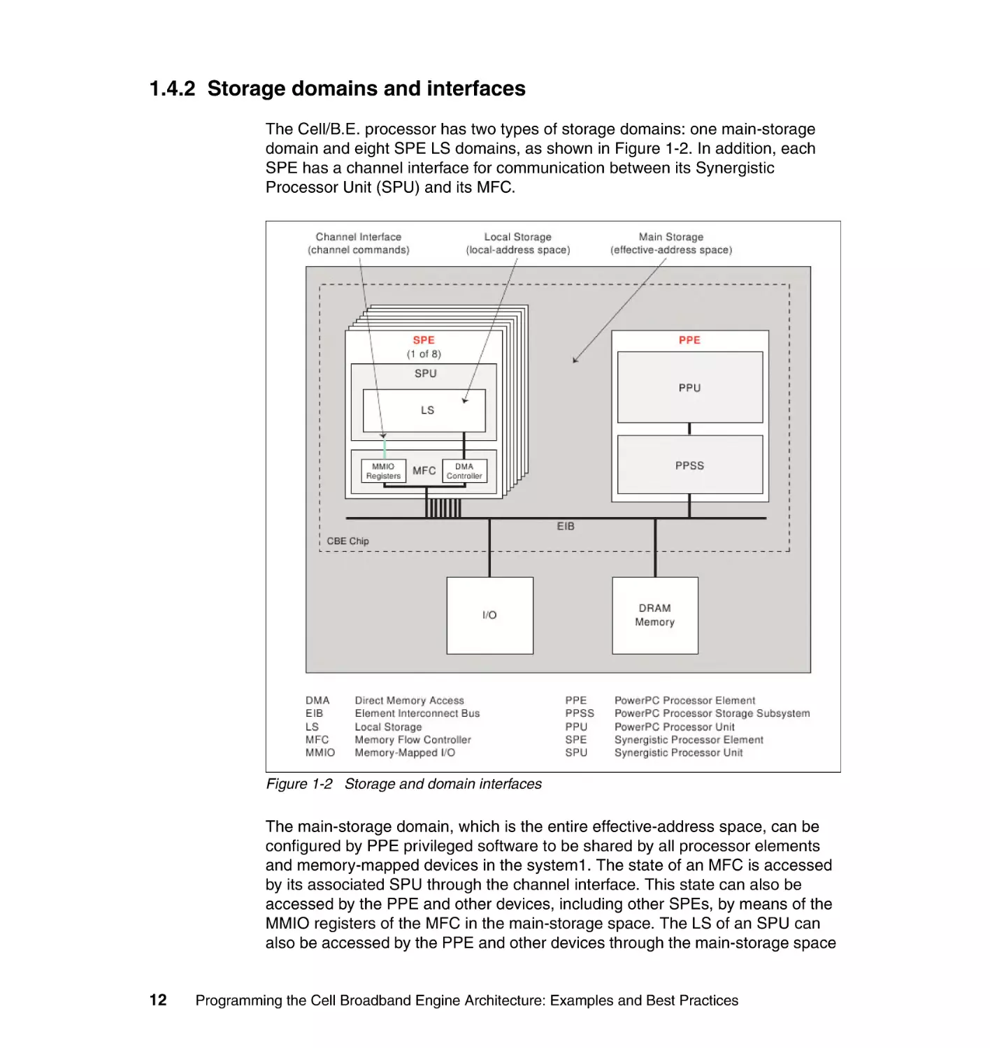
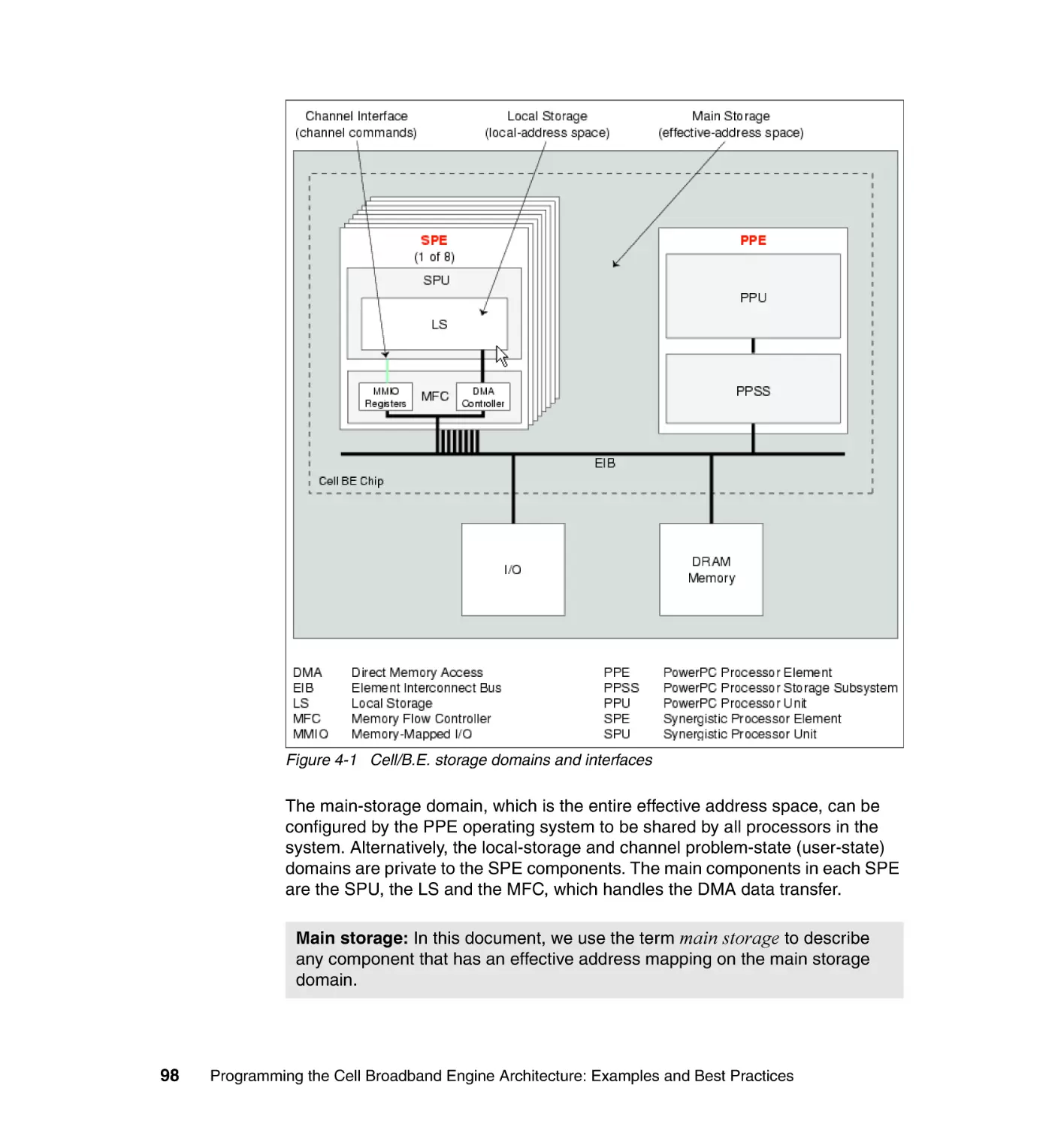
1.4.2 Storage domains and interfaces
The Cell/B.E. processor has two types of storage domains: one main-storage
domain and eight SPE LS domains, as shown in Figure 1-2. In addition, each
SPE has a channel interface for communication between its Synergistic
Processor Unit (SPU) and its MFC.
Figure 1-2 Storage and domain interfaces
The main-storage domain, which is the entire effective-address space, can be
configured by PPE privileged software to be shared by all processor elements
and memory-mapped devices in the system1. The state of an MFC is accessed
by its associated SPU through the channel interface. This state can also be
accessed by the PPE and other devices, including other SPEs, by means of the
MMIO registers of the MFC in the main-storage space. The LS of an SPU can
also be accessed by the PPE and other devices through the main-storage space
12
Programming the Cell Broadband Engine Architecture: Examples and Best Practices
in a non-coherent manner. The PPE accesses the main-storage space through
its PowerPC processor storage subsystem (PPSS).
The address-translation mechanisms used in the main-storage domain are
described in Section 4, “Virtual Storage Environment,” of Cell Broadband Engine
Programming Handbook, Version 1.1.2 In this same document, you can find a
description of the channel domain in Section 19, “DMA Transfers and
Interprocessor Communication.” The SPU of an SPE can fetch instructions only
from its own LS, and load and store instructions executed by the SPU can only
access the LS. SPU software uses LS addresses, not main storage effective
addresses, to do this. The MFC of each SPE contains a DMA controller. DMA
transfer requests contain both an LS address and an effective address, thereby
facilitating transfers between the domains.
Data transfer between an SPE local storage and main storage is performed by
the MFC that is local to the SPE. Software running on an SPE sends commands
to its MFC by using the private channel interface. The MFC can also be
manipulated by remote SPEs, the PPE, or I/O devices by using memory mapped
I/O. Software running on the associated SPE interacts with its own MFC through
its channel interface. The channels support enqueueing of DMA commands and
other facilities, such as mailbox and signal-notification messages. Software
running on the PPE or another SPE can interact with an MFC through MMIO
registers, which are associated with the channels and visible in the main-storage
space.
Each MFC maintains and processes two independent command queues for DMA
and other commands: one queue for its associated SPU and another queue for
other devices that access the SPE through the main-storage space. Each MFC
can process multiple in-progress DMA commands. Each MFC can also
autonomously manage a sequence of DMA transfers in response to a DMA list
command from its associated SPU (but not from the PPE or other SPEs). Each
DMA command is tagged with a tag group ID that allows software to check or
wait on the completion of commands in a particular tag group.
The MFCs support naturally aligned DMA transfer sizes of 1, 2, 4, or 8 bytes, and
multiples of 16 bytes, with a maximum transfer size of 16 KB per DMA transfer.
DMA list commands can initiate up to 2,048 such DMA transfers. Peak transfer
performance is achieved if both the effective addresses and the LS addresses
are 128-byte aligned and the size of the transfer is an even multiple of 128 bytes.
Each MFC has a synergistic memory management (SMM) unit that processes
address-translation and access-permission information that is supplied by the
2
Cell Broadband Engine Programming Handbook, Version 1.1 is available at the following Web
address: http://www-01.ibm.com/chips/techlib/techlib.nsf/techdocs/
9F820A5FFA3ECE8C8725716A0062585F/$file/CBE_Handbook_v1.1_24APR2007_pub.pdf
Chapter 1. Cell Broadband Engine overview
13
PPE operating system. To process an effective address provided by a DMA
command, the SMM uses essentially the same address translation and
protection mechanism that is used by the memory management unit (MMU) in
the PPSS of the PPE. Thus, DMA transfers are coherent with respect to system
storage, and the attributes of system storage are governed by the page and
segment tables of the PowerPC Architecture.
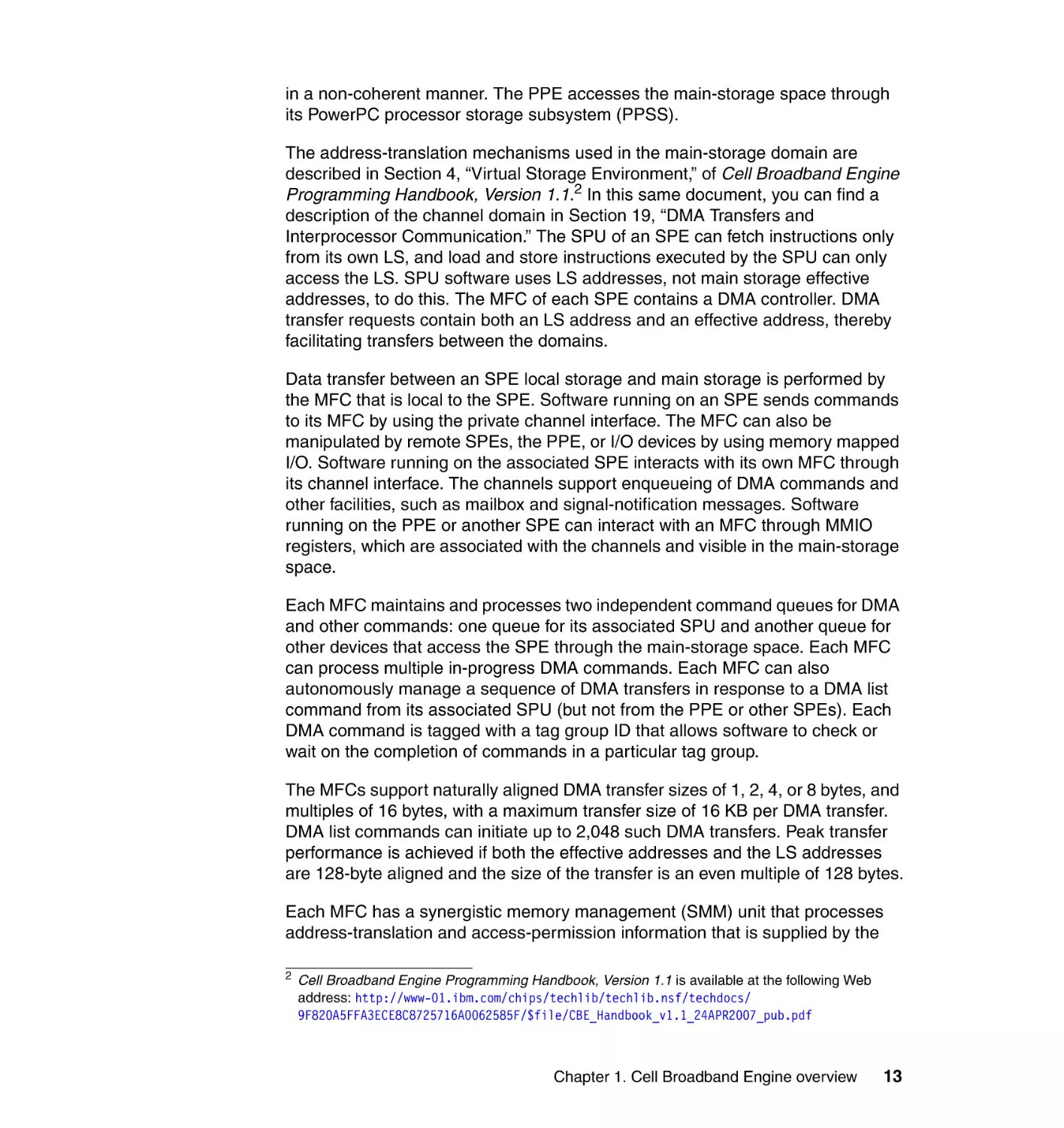
1.4.3 Bit ordering and numbering
Storage of data and instructions in the Cell/B.E. processor uses big-endian
ordering, which has the following characteristics:
The most-significant byte is stored at the lowest address, and the
least-significant byte is stored at the highest address.
Bit numbering within a byte goes from most-significant bit (bit 0) to
least-significant bit (bit n).
This differs from other big-endian processors.
Figure 1-3 shows a summary of the byte ordering and bit ordering in memory
and the bit-numbering conventions.
Figure 1-3 Big-endian byte and bit ordering
Neither the PPE nor the SPEs, including their MFCs, support little-endian byte
ordering. The DMA transfers of the MFC are simply byte moves, without regard
to the numeric significance of any byte. Thus, the big-endian or little-endian issue
becomes irrelevant to the movement of a block of data. The byte-order mapping
only becomes significant when data is loaded or interpreted by a processor
element or an MFC.
14
Programming the Cell Broadband Engine Architecture: Examples and Best Practices
1.4.4 Runtime environment
The PPE runs PowerPC Architecture applications and operating systems, which
can include both PowerPC Architecture instructions and vector/SIMD multimedia
extension instructions. To use all of the Cell/B.E. processor’s features, the PPE
requires an operating system that supports these features, such as
multiprocessing with the SPEs, access to the PPE vector/SIMD multimedia
extension operations, the Cell/B.E. interrupt controller, and all the other functions
provided by the Cell/B.E. processor.
A main thread running on the PPE can interact directly with an SPE thread
through the LS of the SPE. The thread can interact indirectly through the
main-storage space. A thread can poll or sleep while waiting for SPE threads.
The PPE thread can also communicate through mailbox and signal events that
are implemented in the hardware.
The operating system defines the mechanism and policy for selecting an
available SPE to schedule an SPU thread to run on. It must prioritize among all
the Cell/B.E. applications in the system, and it must schedule SPE execution
independently from regular main threads. The operating system is also
responsible for runtime loading, the passing of parameters to SPE programs,
notification of SPE events and errors, and debugger support.
Chapter 1. Cell Broadband Engine overview
15
16
Programming the Cell Broadband Engine Architecture: Examples and Best Practices
2
Chapter 2.
IBM SDK for Multicore
Acceleration
In this chapter, we describe the software tools and libraries that are found in the
Cell Broadband Engine (Cell/B.E.) Software Development Kit (SDK). We briefly
discuss the following topics:
2.1, “Compilers” on page 18
2.2, “IBM Full System Simulator” on page 19
2.3, “Linux kernel” on page 20
2.4, “Cell/B.E. libraries” on page 21
2.5, “Code examples and example libraries” on page 23
2.6, “Performance tools” on page 24
2.7, “IBM Eclipse IDE for the SDK” on page 26
2.8, “Hybrid-x86 programming model” on page 26
© Copyright IBM Corp. 2008. All rights reserved.
17
2.1 Compilers
A number of IBM compilers are supplied as part of the SDK for Multicore
Acceleration. In the following sections, we briefly describe the IBM product
compilers and open source compilers in the SDK.
2.1.1 GNU toolchain
The GNU toolchain, including compilers, the assembler, the linker, and
miscellaneous tools, is available for both the PowerPC Processor Unit (PPU) and
Synergistic Processor Unit (SPU) instruction set architectures. On the PPU, it
replaces the native GNU toolchain, which is generic for the PowerPC
Architecture, with a version that is tuned for the Cell/B.E. PPU processor core.
The GNU compilers are the default compilers for the SDK.
The GNU toolchains run natively on Cell/B.E. hardware or as cross-compilers on
PowerPC or x86 machines.
2.1.2 IBM XLC/C++ compiler
IBM XL C/C++ for Multicore Acceleration for Linux is an advanced,
high-performance cross-compiler that is tuned for the Cell Broadband Engine
Architecture (CBEA). The XL C/C++ compiler, which is hosted on an x86, IBM
PowerPC technology-based system, or an IBM BladeCenter QS21, generates
code for the PPU or SPU. The compiler requires the GCC toolchain for the
CBEA, which provides tools for cross-assembling and cross-linking applications
for both the PowerPC Processor Element (PPE) and Synergistic Processor
Element (SPE).
OpenMP compiler: The IBM XLC/C++ compiler that comes with SDK 3 is an
OpenMP directed single source compiler that supports automatic program
partitioning, data virtualization, code overlay, and more. This version of the
compiler is in beta mode. Therefore, users should not base production
applications on this compiler.
2.1.3 GNU ADA compiler
The GNU toolchain also contains an implementation of the GNU ADA compiler.
This compiler comes in an existing Cell/B.E. processor and an x86
cross-compiler. The initial version of this compiler supports code generation for
the PPU processor.
18
Programming the Cell Broadband Engine Architecture: Examples and Best Practices
2.1.4 IBM XL Fortran for Multicore Acceleration for Linux
IBM XL Fortran for Multicore Acceleration for Linux is the latest addition to the
IBM XL family of compilers. It adopts proven high-performance compiler
technologies that are used in its compiler family predecessors. It also adds new
features that are tailored to exploit the unique performance capabilities of
processors that are compliant with the new CBEA.
This version of XL Fortran is a cross-compiler. First, you compile your
applications on an IBM System p™ compilation host running Red Hat Enterprise
Linux (RHEL) 5.1. Then you move the executable application produced by the
compiler onto a Cell/B.E. system that is also running the RHEL 5.1 Linux
distribution. The Cell/B.E. system is the execution host where you run your
compiled application.
2.2 IBM Full System Simulator
The IBM Full System Simulator (referred to as the simulator in this chapter) is a
software application that emulates the behavior of a full system that contains a
Cell/B.E. processor. You can start a Linux operating system on the simulator,
simulate a two chip Cell/B.E. environment, and run applications on the simulated
operating system. The simulator also supports the loading and running of
statically-linked executable programs and stand-alone tests without an
underlying operating system. Other functions, such as debug output, are not
available on the hardware.
The simulator infrastructure is designed for modeling the processor and
system-level architecture at levels of abstraction, which vary from functional to
performance simulation models with several hybrid fidelity points in between:
Functional-only simulation
This type of simulation models the program-visible effects of instructions
without modeling the time it takes to run these instructions. Functional-only
simulation assumes that each instruction can be run in a constant number of
cycles. Memory accesses are synchronous and are performed in a constant
number of cycles.
This simulation model is useful for software development and debugging
when a precise measure of execution time is not significant. Functional
simulation proceeds much more rapidly than performance simulation, and
therefore, is useful for fast-forwarding to a specific point of interest.
Chapter 2. IBM SDK for Multicore Acceleration
19
Performance simulation
For system and application performance analysis, the simulator provides
performance simulation (also referred to as timing simulation). A
performance simulation model represents internal policies and mechanisms
for system components, such as arbiters, queues, and pipelines.
Operation latencies are modeled dynamically to account for both processing
time and resource constraints. Performance simulation models have been
correlated against hardware or other references to acceptable levels of
tolerance.
The simulator for the Cell/B.E. processor provides a cycle-accurate SPU core
model that can be used for performance analysis of computationally-intense
applications.
2.2.1 System root image for the simulator
The system root image for the simulator is a file that contains a disk image of
Fedora files, libraries, and binaries that can be used within the system simulator.
This disk image file is preloaded with a full range of Fedora utilities and includes
all of the Cell/B.E. Linux support libraries.
2.3 Linux kernel
For the IBM BladeCenter QS21 blade server, the kernel is installed into the /boot
directory, yaboot.conf is modified, and a reboot is required to activate this kernel.
The cellsdk installation task is documented in the Cell Broadband Engine
Software Development Kit 2.1 Installation Guide Version 2.1, SC33-8323-02.1
1
20
Cell Broadband Engine Software Development Kit 2.1 Installation Guide Version 2.1,
SC33-8323-02, is available on the Web at:
ftp://ftp.software.ibm.com/systems/support/bladecenter/cpbsdk00.pdf
Programming the Cell Broadband Engine Architecture: Examples and Best Practices
2.4 Cell/B.E. libraries
In the following sections, we describe various the programming libraries.
2.4.1 SPE Runtime Management Library
The SPE Runtime Management Library (libspe) constitutes the standardized
low-level application programming interface (API) for application access to the
Cell/B.E. SPEs. This library provides an API to manage SPEs that are neutral
with respect to the underlying operating system and its methods.
Implementations of this library can provide additional functionality that allows for
access to operating system or implementation-dependent aspects of SPE
runtime management. These capabilities are not subject to standardization.
Their use may lead to non-portable code and dependencies on certain
implemented versions of the library.
2.4.2 SIMD Math Library
The traditional math functions are scalar instructions and do not take advantage
of the powerful single instruction, multiple data (SIMD) vector instructions that
are available in both the PPU and SPU in the CBEA. SIMD instructions perform
computations on short vectors of data in parallel, instead of on individual scalar
data elements. They often provide significant increases in program speed
because more computation can be done with fewer instructions.
2.4.3 Mathematical Acceleration Subsystem libraries
The Mathematical Acceleration Subsystem (MASS) consists of libraries of
mathematical intrinsic functions, which are tuned specifically for optimum
performance on the Cell/B.E. processor. Currently the 32-bit, 64-bit PPU, and
SPU libraries are supported.
These libraries offer the following advantages:
Include both scalar and vector functions, are thread-safe, and support both
32-bit and 64-bit compilations
Offer improved performance over the corresponding standard system library
routines
Are intended for use in applications where slight differences in accuracy or
handling of exceptional values can be tolerated
Chapter 2. IBM SDK for Multicore Acceleration
21
2.4.4 Basic Linear Algebra Subprograms
The Basic Linear Algebra Subprograms (BLAS) library is based upon a published
standard interface for commonly used linear algebra operations in
high-performance computing (HPC) and other scientific domains. It is widely
used as the basis for other high quality linear algebra software, for example
LAPACK and ScaLAPACK. The Linpack (HPL) benchmark largely depends on a
single BLAS routine (DGEMM) for good performance.
The BLAS API is available as standard ANSI C and standard FORTRAN 77/90
interfaces. BLAS implementations are also available in open source (netlib.org).
The BLAS library in IBM SDK for Multicore Acceleration supports only real
single-precision (SP) and real double-precision (DP) versions. All SP and DP
routines in the three levels of standard BLAS are supported on the PPE. These
routines are available as PPE APIs and conform to the standard BLAS interface.
Some of these routines are optimized by using the SPEs and show a marked
increase in performance compared to the corresponding versions that are
implemented solely on the PPE. These optimized routines have an SPE interface
in addition to the PPE interface. The SPE interface does not conform to, yet
provides a restricted version of, the standard BLAS interface. Moreover, the single
precision versions of these routines have been further optimized for maximum
performance by using various features of the SPE.
2.4.5 ALF library
The Accelerated Library Framework (ALF) provides a programming environment
for data and task parallel applications and libraries. The ALF API provides library
developers with a set of interfaces to simplify library development on
heterogenous multi-core systems. Library developers can use the provided
framework to offload computationally intensive work to the accelerators. More
complex applications can be developed by combining the several function offload
libraries. Application programmers can also choose to implement their
applications directly to the ALF interface.
The ALF supports the multiple-program-multiple-data (MPMD) programming
module where multiple programs can be scheduled to run on multiple accelerator
elements at the same time.
The ALF library includes the following functionality:
Data transfer management
Parallel task management
Double buffering and dynamic load balancing
22
Programming the Cell Broadband Engine Architecture: Examples and Best Practices
2.4.6 Data Communication and Synchronization library
The Data Communication and Synchronization (DaCS) library provides a set of
services for handling process-to-process communication in a heterogeneous
multi-core system. In addition to the basic message passing service, the library
includes the following services:
Mailbox services
Resource reservation
Process and process group management
Process and data synchronization
Remote memory services
Error handling
The DaCS services are implemented as a set of APIs that provide an
architecturally neutral layer for application developers. They structure the
processing elements, referred to as DaCS elements (DE), into a hierarchical
topology. This includes general purpose elements, referred to as host elements
(HE), and special processing elements, referred to as accelerator elements (AE).
HEs usually run a full operating system and submit work to the specialized
processes that run in the AEs.
2.5 Code examples and example libraries
The example libraries package provides a set of optimized library routines that
greatly reduce the development cost and enhance the performance of Cell/B.E.
programs. To demonstrate the versatility of the CBEA, a variety of
application-oriented libraries are included, such as the following libraries:
Fast Fourier Transform (FFT)
Image processing
Software managed cache
Game math
Matrix operation
Multi-precision math
Synchronization
Vector
Additional examples and demonstrations show how you can exploit the on-chip
computational capacity.
Chapter 2. IBM SDK for Multicore Acceleration
23
2.6 Performance tools
The Cell/B.E. SDK supports many of the traditional Linux-based performance
tools that are available. The performance tools, such as gprof, pertain specifically
to the PPE execution environment and do not support the SPE environment. The
tools in the following sections are special tools that support the PPE, SPE, or
both types of environments.
2.6.1 SPU timing tool
The SPU static timing tool, spu_timing, annotates an SPU assembly file with
scheduling, timing, and instruction issue estimates assuming a straight, linear
execution of the program, which is useful for analyzing basic code blocks. The
tool generates a textual output of the execution pipeline of the SPE instruction
stream from this input assembly file. The output generated can show pipeline
stalls, which can be explained by looking at the subsequent instructions. Data
dependencies are pipeline hazards that can be readily identified by using this
tool.
Lastly, this is a static analysis tool. It does not identify branch behavior or
memory transfer delays.
2.6.2 OProfile
OProfile is a Linux tool that exists on other architectures besides the Cell/B.E. It
has been extended to support the unique hardware on the PPU and SPUs. It is a
sampling based tool that does not require special source compile flags to
produce useful data reports.
The opreport tool produces the output report. Reports can be generated based
on the file names that correspond to the samples, symbol names, or annotated
source code listings. Special source compiler flags are required in this case.
2.6.3 Cell-perf-counter tool
The cell-perf-counter (cpc) tool is used for setting up and using the hardware
performance counters in the Cell/B.E. processor. These counters allow you to
see how many times certain hardware events are occurring, which is useful if you
are analyzing the performance of software running on a Cell/B.E. system.
Hardware events are available from all of the logical units within the Cell/B.E.
processor, including the PPE, SPEs, interface bus, and memory and I/O
controllers. Four 32-bit counters, which can also be configured as pairs of 16-bit
24
Programming the Cell Broadband Engine Architecture: Examples and Best Practices
counters, are provided in the Cell/B.E. performance monitoring unit (PMU) for
counting these events.
2.6.4 Performance Debug Tool
The Cell/B.E. Performance Debug Tool (PDT) provides programmers with a
means of analyzing the execution of such a system and tracking problems in
order to optimize execution time and utilization of resources. The PDT addresses
performance debugging of one Cell/B.E. board with two PPEs that share the
main memory, run under the same (Linux) operating system, and share up to 16
SPEs. The PDT also enables event tracing on the Hybrid-x86.
2.6.5 Feedback Directed Program Restructuring tool
The Feedback Directed Program Restructuring (FDPR-Pro or fdprpro) tool for the
Linux on Power is a performance tuning utility that reduces the execution time
and the real memory utilization of user space application programs. It optimizes
the executable image of a program by collecting information about the behavior
of the program under a workload. It then creates a new version of that program
that is optimized for that workload. The new program typically runs faster and
uses less real memory than the original program and supports the Cell/B.E.
environment.
2.6.6 Visual Performance Analyzer
Visual Performance Analyzer (VPA) is an Eclipse-based performance
visualization toolkit. It consists of six major components:
Profile Analyzer
Code Analyzer
Pipeline Analyzer
Counter Analyzer
Trace Analyzer
Control Flow Analyzer
Profile Analyzer provides a powerful set of graphical and text-based views. By
using these views, users can narrow down performance problems to a particular
process, thread, module, symbol, offset, instruction, or source line. Profile
Analyzer supports time-based system profiles (Tprofs) that are collected from a
number of IBM platforms and the Linux profile tool oprofile. The Cell/B.E.
platform is now a fully supported environment for VPA.
Chapter 2. IBM SDK for Multicore Acceleration
25
2.7 IBM Eclipse IDE for the SDK
IBM Eclipse IDE for the SDK is built upon the Eclipse and C Development Tools
(CDT) platform. It integrates the GNU toolchain, compilers, the Full System
Simulator, and other development components to provide a comprehensive,
Eclipse-based development platform that simplifies development. Eclipse IDE for
the SDK includes the following key features:
A C/C++ editor that supports syntax highlighting, a customizable template,
and an outline window view for procedures, variables, declarations, and
functions that appear in source code
A visual interface for the PPE and SPE combined GDB (GNU debugger) and
seamless integration of the simulator into Eclipse
Automatic builder, performance tools, and several other enhancements;
remote launching, running and debugging on a BladeCenter QS21; and ALF
source code templates for programming models within IDE
An ALF Code Generator to produce an ALF template package with C source
code and a readme.txt file
A configuration option for both the Local Simulator and Remote Simulator
target environments so that you can choose between launching a simulation
machine with the Cell/B.E. processor or an enhanced CBEA-compliant
processor with a fully pipelined, double precision SPE processor
Remote Cell/B.E. and simulator BladeCenter support
SPU timing integration and automatic makefile generation for both GCC and
XLC projects
2.8 Hybrid-x86 programming model
The CBEA is an example of a multi-core hybrid system on a chip. Heterogeneous
cores are integrated on a single processor with an inherent memory hierarchy.
Specifically, the SPEs can be thought of as computational accelerators for a
more general purpose PPE core. These concepts of hybrid systems, memory
hierarchies, and accelerators can be extended more generally to coupled I/O
devices. Such systems exist today, such as GPUs in Peripheral Component
Interconnect Express (PCIe) slots for workstations and desktops.
Similarly, the Cell/B.E. processor is used in systems as an accelerator, where
computationally intensive workloads that are well suited for the CBEA are
off-loaded from a more standard processing node. There are potentially many
26
Programming the Cell Broadband Engine Architecture: Examples and Best Practices
ways to move data and functions from a host processor to an accelerator
processor and vice versa.
The SDK has implementations of the Cell/B.E. multi-core data communication
and programming model libraries, DaCS and ALF, which can be used on x86 or
Linux host process systems with Cell/B.E.-based accelerators. They provide a
consistent methodology and set of APIs for a variety of hybrid systems, including
the Cell/B.E. SoC hybrid system. The current implementation is over TCP/IP
sockets and is provided so that you can gain experience with this programming
style and focus on how to manage the distribution of processing and data
decomposition. For example, in the case of hybrid programming when moving
data point to point over a network, use care to maximize the computational work
done on accelerator nodes potentially with asynchronous or overlapping
communication, given the potential cost in communicating input and results.
Chapter 2. IBM SDK for Multicore Acceleration
27
28
Programming the Cell Broadband Engine Architecture: Examples and Best Practices
Part 2
Part
2
Programming
environment
In this part, we provide in-depth coverage of various programming methods,
tools, strategies, and adaptions to different computing workloads. Specifically this
part includes the following chapters:
Chapter 3, “Enabling applications on the Cell Broadband Engine hardware”
on page 31
Chapter 4, “Cell Broadband Engine programming” on page 75
Chapter 5, “Programming tools and debugging techniques” on page 329
Chapter 6, “The performance tools” on page 417
Chapter 7, “Programming in distributed environments” on page 445
© Copyright IBM Corp. 2008. All rights reserved.
29
30
Programming the Cell Broadband Engine Architecture: Examples and Best Practices
3
Chapter 3.
Enabling applications on the
Cell Broadband Engine
hardware
In this chapter, we describe the process of enabling an existing application on the
Cell Broadband Engine (Cell/B.E.) hardware. The goal is to provide guidance for
choosing the best programming model and framework for a given application.
This is valuable information for people who develop applications and for IT
specialists who must manage a Cell/B.E. application enablement project.
We include an example of a completely new application that is written from
scratch. You can consider this example as a case of application enablement,
where the starting point is not the actual code, but the algorithms with no initial
data layout decisions. In a sense, this is an easier way because the options are
completely open and not biased by the current state of the code.
In this chapter, we answer the following questions:
Should we enable this application on the Cell/B.E. hardware? Is it a good fit?
If the answer to the previous question is “yes,” then which parallel
programming model should we use? The Cell Broadband Engine Architecture
(CBEA), with its heterogenous design and software controlled memory
© Copyright IBM Corp. 2008. All rights reserved.
31
hierarchy, offers new parallel programming paradigms to complement the well
established ones.
Which Cell/B.E. programming framework will best support the programming
model that was chosen for the application under study?
After we answer these questions, we make the necessary code changes to
exploit the CBEA. We describe this process and show that it can be iterative and
incremental, which are two interesting features. Considering these features, we
can use a step-by-step approach, inserting checkpoints during the course of the
porting project to track the progress. Finally, we present scenarios and make a
first attempt at creating a set of design patterns for Cell/B.E. programming.
In this chapter, we begin by defining the concepts and terminology. We introduce
the following concepts:
The computational kernels frequently found in applications
The distinctive features of the CBEA, which are covered in detail in Chapter 4,
“Cell Broadband Engine programming” on page 75
The parallel programming models
The Cell/B.E. programming frameworks, which are described in Chapter 4,
“Cell Broadband Engine programming” on page 75, and Chapter 7,
“Programming in distributed environments” on page 445
Next we describe the relationship between the computational kernels and the
Cell/B.E. features and between parallel programming models and Cell/B.E.
programming frameworks. We give examples of the most common parallel
programming models and contrast them in terms of control parallelism and data
transfers. We also present design patterns for Cell/B.E. programming following a
formalism used in other areas of computer sciences.
Specifically, this chapter includes the following sections:
3.1, “Concepts and terminology”
3.2, “Determining whether the Cell/B.E. system fits the application
requirements” on page 48
3.3, “Deciding which parallel programming model to use” on page 53
3.4, “Deciding which Cell/B.E. programming framework to use” on page 61
3.5, “The application enablement process” on page 63
3.6, “A few scenarios” on page 66
3.7, “Design patterns for Cell/B.E. programming” on page 70
32
Programming the Cell Broadband Engine Architecture: Examples and Best Practices
3.1 Concepts and terminology
Figure 3-1 shows the concepts and how they are related. As described in this
section, the figure shows an application as having one or more computational
kernels and one or more potential parallel programming models. The
computational kernels exercise or stress one or more of the Cell/B.E. features
(the Q1 connection). The different Cell/B.E. features can either strongly or weakly
support the different parallel programming model choices (the Q2 connection).
The chosen parallel programming model can be implemented on the CBEA by
using various programming frameworks (the Q3 connection).
To answer questions Q1 and Q2, the programmer must be able to match the
characteristics of the computational kernel and parallel programming model to
the strengths of the CBEA. Many programming frameworks are available for the
CBEA. Which one is best suited to implement the parallel programming model
that is chosen for the application? We provide advice to the programmer for
question Q3 in 3.4, “Deciding which Cell/B.E. programming framework to use” on
page 61.
Figure 3-1 Overview of programming considerations and relations
Chapter 3. Enabling applications on the Cell Broadband Engine hardware
33
3.1.1 The computation kernels
A study by David Patterson et al. in The Landscape of Parallel Computing
Research: A View from Berkeley [1 on page 623], complements earlier work from
Phillip Colella [8 on page 624]. Patterson et al. establish that the computational
characteristics and data movement patterns of all applications in scientific
computing, embedded computing, and desktop and server computing can be
captured by no more than thirteen different kernels. They call them the “13
dwarfs” in their paper.1
This work is based on a careful examination of the most popular benchmark
suites:
Embedded Microprocessor Benchmark Consortium (EEMBC) for the
embedded computing
Standard Performance Evaluation Consortium (SPEC) int and fp for desktop
and server computing
High Performance Computing Challenge (HPCC) and NASA Advanced
Supercomputing (NAS) parallel benchmarks for scientific computing,
This work is also based on input from other domains including machine learning,
database, computer graphics, and games. The first seven dwarfs are the ones
that were initially found by Phillip Colella. The six remaining ones were identified
by Patterson et al. The intent of the study is to help the parallel computing
research community, in both academia and the industry, by providing a limited set
of patterns against which new ideas for hardware and software can be evaluated.
We describe the “13 dwarfs” in Table 3-1, with example applications or
benchmarks. This table is adapted from The Landscape of Parallel Computing
Research: A View from Berkeley [1 on page 623].
Table 3-1 Description and examples of the 13 dwarfs
1
34
Dwarf name
Description
Example, application,
benchmark
Dense matrices
Basic Linear Algebra
Subprograms (BLAS),
matrix-matrix operations
HPCC:HPL, ScaLAPACK,
NAS:LU
Sparse matrices
Matrix-vector operations with
sparse matrices
SuperLU, SpMV, NAS:CG
Spectral methods
Fast Fourier Transform (FFT)
HPCC:FFT, NAS:FT,
FFTW
Intel also classifies applications in three categories named RMS for Recognition, Mining and
Synthesis to direct its research in computer architecture. See 9 on page 624.
Programming the Cell Broadband Engine Architecture: Examples and Best Practices
Dwarf name
Description
Example, application,
benchmark
N-body methods
Interactions between particles,
external, near and far
NAMD, GROMACS
Structured grids
Regular grids, can be
automatically refined
WRF, Cactus, NAS:MG
Unstructured grids
Irregular grids, finite elements
and nodes
ABAQUS, FIDAP (Fluent)
Map-reduce
Independent data sets, simple
reduction at the end
Monte-Carlo, NAS:EP, Ray
tracing
Combinatorial logic
Logical functions on large data
sets, encryption
AES, DES
Graph traversal
Decision tree, searching
XML parsing, Quicksort
Dynamic programming
Hidden Markov models,
sequence alignment
BLAST
Back-track and
Branch+Bound
Constraint optimization
Simplex algorithm
Graphical models
Hidden Markov models,
Bayesian networks
HMMER, bioinformatics,
genomics
Finite state machine
XML transformation, Huffman
decoding
SPECInt:gcc
During the course of writing The Landscape of Parallel Computing Research: A
View from Berkeley [1 on page 623], IBM provided an additional classification for
the 13 dwarfs. IBM did this by evaluating that factor that was often limiting its
performance, whether it was the processor, memory latency, or memory
bandwidth. Table 3-2 is extracted from that paper.
Table 3-2 Performance bottlenecks of the 13 dwarfs
Dwarf
Performance bottleneck (processor, memory
bandwidth, memory latency
Dense matrices
Processor limited
Sparse matrices
Processor limited 50%, bandwidth limited 50%
Spectral methods
Memory latency limited
N-body methods
Processor limited
Structured grids
Memory bandwidth limited
Chapter 3. Enabling applications on the Cell Broadband Engine hardware
35
Dwarf
Performance bottleneck (processor, memory
bandwidth, memory latency
Unstructured grids
Memory latency limited
Map-reduce
(Unknown)a
Combinatorial logic
Memory bandwidth limited for CRC, processor
limited for cryptography
Graph traversal
Memory latency limited
Dynamic programming
Memory latency limited
Back-track and Branch+Bound
(Unknown)
Graphical models
(Unknown)
Finite state machine
(Unknown)
a. Every method will ultimately have a performance bottleneck of some kind. At the time of
writing, specific performance bottlenecks for these “unknown” computational kernel types
as applied to the Cell/B.E. platform are well understood.
The Cell/B.E. platform brings improvements in all three directions:
Nine cores on a chip represent a lot of processor power.
The extreme data rate (XDR) memory subsystem is extremely capable.
The software managed memory hierarchy (direct memory access (DMA)) is a
new way of dealing with the memory latency problem, quoted in the paper as
the most critical one.
3.1.2 Important Cell/B.E. features
In this section, we consider features that are meaningful from an application
programmer’s point of view. Referring to Table 3-3 on page 37, the column
labelled “Not so good” only means that the feature is probably going to cause
problems for the programmer or that code that exercises this feature a lot will not
perform as fast as expected. The difference between the “Good” and “Not so
good” columns is also related to the relative performance advantage of the
Cell/B.E. platform over contemporary processors from IBM or others. This
analysis is based on current hardware implementation at the time this book was
written.
This table is likely to change with future products. Most of the items in the table
are described in detail in Chapter 4, “Cell Broadband Engine programming” on
page 75.
36
Programming the Cell Broadband Engine Architecture: Examples and Best Practices
Table 3-3 Important Cell/B.E. features as seen from a programmer’s perspective
Good
Not so good
Large register file
DMA (memory latency hiding)a
DMA latency
Element interconnect bus (EIB) bandwidth b
Memory performance
Memory size
Single-instruction, multiple-data (SIMD)c
Scalar performance (scalar on vector)
Local storage (latency/bandwidth)
Local storage (limited size)
Eight Synergistic Processor Element (SPE)
per processor (high level of achievable
parallelism)
Power Processor Element (PPE)
performance
Nonuniform memory access (NUMA; good
scaling)
Symmetric multiprocessor (SMP)
scaling
Branching
Single precision floating point
Double precision floating pointd
a. See 4.3, “Data transfer” on page 110.
b. See 4.3.4, “Direct problem state access and LS-to-LS transfer” on page 144.
c. See 4.6.4, “SIMD programming” on page 258.
d. This is expected to improve with the introduction of the BladeCenter QS-22.
Peak performance: In general, the percentage of peak performance that can
be achieved on the Cell/B.E. platform can be higher than for most general
purpose processors. This percentage is a result of the large register file, the
short local storage latency, the software managed memory hierarchy, the high
EIB bandwidth, and the capable memory subsystem.
3.1.3 The parallel programming models
The parallel programming models abstract the hardware for the application
programmers. The purpose is to offer an idealized view of the current system
architectures, a view onto which applications can be mapped as shown in
Figure 3-2 on page 38.
Chapter 3. Enabling applications on the Cell Broadband Engine hardware
37
Figure 3-2 The programming model
A parallel application tries to bind multiple resources for its own use, which may
be in regard to memory and processors. The purpose is either to speed up the
whole computation (more processors) or to treat bigger problems (more
memory). The work of parallelizing an application involves the following tasks:
Distributing the work across processors
Distributing the data if the memory is distributed
Synchronizing the subtasks, possibly through shared data access if the
memory is shared
Communicating the data if the memory is distributed
Let us look at the options for each of these components in the following sections.
38
Programming the Cell Broadband Engine Architecture: Examples and Best Practices
Work distribution
The first task is to find concurrency in the application by exposing multiple
independent tasks and grouping them together inside execution threads. The
following options are possible:
Independent tasks operating on largely independent data
Domain decomposition, where the whole data can be split in multiple
subdomains, each of which is assigned to a single task
Streaming, where the same piece of data undergoes successive
transformations, each of which is performed by a single task
All tasks are arranged in a string and pass data in a producer-consumer
mode. The amount of concurrency here is the number of different steps in the
computation.
Now each parallel task can perform the work itself, or it can call other processing
resources for assistance. This process is completely transparent to the rest of the
participating tasks. We find the following techniques:
Function offload, where the compute-intensive part of the job is offloaded to a
supposedly faster processor
Accelerator mode, which is a variant of the previous technique, where multiple
processors can be called to collectively speed up the computation
Data distribution
The data model is an important part of the parallelization work. Currently, the
choices are available:
Shared memory, in which every execution thread has direct access to other
threads’ memory contents
Distributed memory, which is the opposite of shared memory in that each
execution thread can only access its own memory space
Specialized functions are required to import other threads’ data into its own
memory space.
Partitioned Global Address Space (PGAS), where each piece of data must be
explicitly declared as either shared or local, but within a unified address space
Task synchronization
Sometimes, during program execution, the parallel tasks must synchronize.
Synchronization can be realized in the following ways:
Messages or other asynchronous events emitted by other tasks
Locks or other synchronization primitives, for example, to access a queue
Transactional memory mechanisms
Chapter 3. Enabling applications on the Cell Broadband Engine hardware
39
Data communication
In the case where the data is distributed, tasks exchange information through
one of the following two mechanisms:
Message passing, using send and receive primitives
Remote DMA (rDMA), which is sometimes defined as one-sided
communication
The programming models can further be classified according to the way each of
these tasks is taken care of, either explicitly by the programmer or implicitly by
the underlying runtime environment. Table 3-4 lists common parallel
programming models and shows how they can be described according to what
was exposed previously.
Table 3-4 Parallel programming models
Programming
modela
Task
distribution
Data
distribution
Task
synchronization
Data
communication
Message passing
interface (MPI)
Explicit
Explicit
Messages
Messages, can do
rDMA too
pthreads
Explicit
N/A
Mutexes, condition
variables
N/A
OpenMP
Implicit
(directives)
N/A
Implicit (directives)
N/A
UPC, CAF (PGAS)
Explicit
Explicit
Implicit
Implicit
X10 (PGAS)
Explicit
Explicit
Future, clocks
Implicit
StreamIt
Explicit
Explicit
Explicit
Implicit
a. Not all of these programming models are available or appropriate for the Cell/B.E. platform.
Programming model composition
An application can use multiple programming models, which incurs additional
efforts but may be dictated by the hardware on which it is to be run. For example,
the MPI and OpenMP combination is quite common today for high-performance
computing (HPC) applications because it matches the Beowulf2 type of clusters,
interconnecting small SMP nodes (4- and 8-way) with a high-speed
interconnection network.
2
40
Clusters based on commodity hardware. See http://www.beowulf.org/overview/index.html
Programming the Cell Broadband Engine Architecture: Examples and Best Practices
In this discussion about the parallel programming models, we ignore the
instruction level (multiple execution units) and word level (SIMD) parallelisms.
They are to be considered as well to maximize the application performance, but
they usually do not interfere with the high level tasks of data and work
distribution.
3.1.4 The Cell/B.E. programming frameworks
The CBEA supports a wide of range of programming frameworks, from the most
basic ones, close to the hardware, to the most abstract ones.
At the lowest level, the Cell/B.E. chip appears to the programmer as a distributed
memory cluster of 8+1 computational cores, with an ultra high-speed
interconnect and a remote DMA engine on every core. On a single blade server,
two Cell/B.E. chips can be viewed as either a single 16+2 cores compute
resource (SMP mode) or a NUMA machine with two NUMA nodes.
Multiple blade servers can then be gathered in a distributed cluster, by using
Beowulf, with a high-speed interconnect network such as a 10G Ethernet or
InfiniBand®. Such a cluster is not any different, in regard to programming, from a
cluster of Intel, AMD™, or IBM POWER™ technology-based SMP servers. It is
likely that the programming model will be based on distributed memory
programming that uses MPI as the communication layer across the blades.
An alternative arrangement is to have Cell/B.E. blade servers serve only as
accelerator nodes for other systems. In this configuration, the application logic is
not managed at the Cell/B.E. level but at the accelerated system level. The dialog
that we are interested in is between the Cell/B.E. level and the system for which it
provides acceleration.
The frameworks that are part of the IBM SDK for Multicore Acceleration are
described in greater detail in 4.7, “Frameworks and domain-specific libraries” on
page 289, and 7.1, “Hybrid programming models in SDK 3.0” on page 446. We
only give a brief overview in the following sections.
libspe2 and newlib
libspe2 and newlib are the lowest possible levels for application programmers. By
using the libspe2 and newlib libraries, programmers deal with each feature of the
Cell/B.E. architecture with full control. libspe2 and newlib offer the following
features:
Chapter 3. Enabling applications on the Cell Broadband Engine hardware
41
SPE context management for creating, running, scheduling, and deleting SPE
contexts
DMA primitives for accessing remote memory locations from the PPE and the
SPEs
Mailboxes, signal, events, and synchronization functions for PPE-SPE and
SPE-SPE dialogs and control
PPE-assisted calls, which is a mechanism to have the PPE service requests
from the SPEs
Important: Libspe2 is a framework for obtaining access to the SPEs. Mailbox,
DMAs, signals, and so on are much faster when using direct problem state.
High performance programs should avoid making frequent libspe2 calls since
they often use kernel services. Therefore, it is best to use libspe2 to get
parallel tasks started and then to use the memory flow controller (MFC)
hardware facilities for application task management, communications, and
synchronization.
By using these libraries, any kind of parallel programming model can be
implemented. libspe2 is described in detail in 4.1, “Task parallelism and PPE
programming” on page 77.
Software cache
A software cache can help implement a shared memory parallel programming
model when the data that the SPEs reference cannot be easily predicted. See
4.3.6, “Automatic software caching on SPE” on page 157, for more details.
Data Communication and Synchronization
Data Communication and Synchronization (DaCS) provides services to multi-tier
applications by using a hierarchy of processing elements. A DaCS program can
be a host element (HE), an accelerator element (AE), or both if multiple levels of
acceleration are needed. An AE can only communicate within the realm of the
HE. An HE does not need to be of the same type as its AEs. This is the hybrid
model. DaCS handles the necessary byte swapping if the data flows from a little
endian machine to a big endian.
DaCS offers the following typical services:
Resource and process management, where an HE manipulates its AEs
Group management, for defining groups within which synchronization events
like barriers can happen
Message passing by using send and receive primitives
42
Programming the Cell Broadband Engine Architecture: Examples and Best Practices
Mailboxes
Remote DMA operations
Process synchronization using barriers
Data synchronization using mutexes to protect memory accesses
The DaCS services are implemented as an API for the Cell/B.E.-only version and
are complemented by a runtime daemon for the hybrid case. For a complete
discussion, see 4.7.1, “Data Communication and Synchronization” on page 291,
and 7.2, “Hybrid Data Communication and Synchronization” on page 449.
MPI
MPI is not part of the IBM SDK for Multicore Acceleration. However, any
implementation for Linux on Power can run on the Cell/B.E., leveraging the PPE
only. The following implementations are the most common:
MPICH/MPICH2, from Argonne National Laboratory
MVAPICH/MVAPICH2, from Ohio State University
OpenMPI, from a large consortium involving IBM and Los Alamos National
Laboratory, among others
There is no difference from a functional point of view between these MPI
implementations running on the Cell/B.E. platform and running on other
platforms. MPI is a widespread standard for writing distributed memory
applications. As opposed to DaCS, MPI treats all tasks as equal. The
programmer can decide later if some tasks are to play a particular role in the
computation. MPI is implemented as an API and a runtime environment to
support all sorts of interconnection mechanisms between the MPI tasks,
including shared memory, sockets for TCP/IP networks, or OpenIB (OFED) for
InfiniBand networks.
Accelerated Library Framework
An Accelerated Library Framework (ALF) program uses multiple ALF accelerator
tasks to perform the compute-intensive part of the work. The idea is to have the
host program split the work into multiple independent pieces, which are called
work blocks. They are described by a computational kernel, the input data they
need, and the output data they produce.
On the accelerator side, the programmer only has to code the computational
kernel, unwrap the input data, and pack the output data when the kernel finishes
processing. In between, the runtime system manages the work blocks queue on
the accelerated side and gives control to the computational kernel upon receiving
a new work block on the accelerator side.
Chapter 3. Enabling applications on the Cell Broadband Engine hardware
43
The ALF imposes a clear separation between the application logic and control
running on the host task from the computational kernels that run on the
accelerator nodes, acting as service providers that are fed with input data and
echo output data in return. The ALF run time provides the following services “for
free” from the application programmer perspective:
Work blocks queue management
Load balancing between accelerators
Transparent DMA transfers, exploiting the data transfer list used to describe
the input and output data
Table 3-5 summarizes the various duties.
Table 3-5 Work separation with ALF
Who
Does what
Host code writer
Program flow logic
Manage accelerators
Work blocks creation, input and output data specified as
a series of address-type-length entries
Manage communication and synchronization with peer
host tasks
Accelerator code writer
Computational kernel
ALF run time
Schedule work blocks to accelerators
Data transfer
The ALF also offers more sophisticated mechanisms for managing multiple
computational kernels or express dependencies, or to further tune the data
movement. As with DaCS, the ALF can operate inside a Cell/B.E. server or in
hybrid mode.
The ALF is described in detail in 4.7.2, “Accelerated Library Framework” on
page 298, and 7.3, “Hybrid ALF” on page 463.
IBM Dynamic Application Virtualization
With Dynamic Application Virtualization (DAV), an IBM alphaWorks offering, an
application can benefit from Cell/B.E. acceleration without any source code
changes. The original, untouched application is directed to use a stub library that
is dynamically loaded and offloads the compute intense functions to a Cell/B.E
system. DAV currently supports C/C++ or Visual Basic® Applications, such as
Microsoft® Excel® 2007 spreadsheets, that run under the Microsoft Windows®
operating system.
44
Programming the Cell Broadband Engine Architecture: Examples and Best Practices
DAV comes with tools to generate ad-hoc stub libraries based on the prototypes
of the offloaded functions on the client side and similar information about the
server side (the Cell/B.E. system) where the functions are implemented. For the
main application, the Cell/B.E. system is completely hidden. The actual
implementation of the function on the Cell/B.E. system uses the existing
programming frameworks to maximize the application performance.
See 7.4, “Dynamic Application Virtualization” on page 475, for a more complete
description.
Workload specific libraries
The IBM SDK for Multicore Acceleration contains workload specialized libraries.
The libraries are the BLAS library for linear algebra, libFFT for FFT in 1D and 2D,
and libmc for random number generations.
OpenMP
The IBM SDK for Multicore Acceleration contains a technology preview of the XL
C/C++ single source compiler. Usage of this compiler completely hides the
Cell/B.E. system to the application programmer who can continue by using
OpenMP, which is a familiar shared memory parallel programming model. The
compiler runtime library takes care of spawning threads of execution on the
SPEs and manages the data movement and synchronization of the PPE threads
to SPE threads.
Other groups or companies are working on providing programming frameworks
for the Cell/B.E. platform as discussed in the following sections.
Mercury Computer Systems
Mercury has two main offerings for the Cell/B.E. platform:
The MultiCore Framework (MCF), which implements the manager/worker
model with an input/output tile management similar to the ALF work blocks
Multicore Plus SDK, which bundles MCF with additional signal processing
and FFT libraries (SAL, Vector Signal and Image Processing Library
(VSIPL)), a trace library (TATL), and open source tools for MPI
communications (OpenMPI) and debugging (gdb)
PeakStream
The PeakStream platform offers an API, a generalize array type, and a virtual
machine environment that abstracts the programmer from the real hardware.
Data is moved back and forth between the application and the virtual machine
that accesses the Cell/B.E. resources by using an I/O interface. All the work in
the virtual machine is asynchronous from the main application perspective, which
can keep doing work before reading the data from the virtual machine. The
Chapter 3. Enabling applications on the Cell Broadband Engine hardware
45
PeakStream platform currently runs on the Cell/B.E. platform, GPUs, and
traditional homogeneous multi-core processors.
CodeSourcery
CodeSourcery offers Sourcery VSIPL++, a C++ implementation of the open
standard VSIPL++ library that is used in signal and image processing. The
programmer is freed from accessing the low level mechanisms of the Cell/B.E.
platform. This is handled by the CodeSourcery runtime library.
The VSIPL contains routines for the following items:
Linear algebra for real and complex values
Random numbers
Signal and image processing (FFT, convolutions, and filters)
CodeSourcery also runs on GPU and a multi-core general purpose processor.
Gedae
Gedae tries to automate the software development by using a model-driven
approach. The algorithm is captured in a flow diagram that is then used by the
multiprocessor compiler to generate a code that will match both the target
architecture and the data movements required by the application.
RapidMind
RapidMind works with standard C++ language constructs and augments the
language by using specialized macro language functions. The whole integration
involves the following steps:
1. Replace float or int arrays by RapidMind equivalent types (Array, Value).
2. Capture the computations that are enclosed between the RapidMind
keywords Program BEGIN and END and convert them into object modules.
3. Stream the recorded computations to the underlying hardware by using
platform-specific constructs, such as Cell/B.E., processor, or GPU, when the
modules are invoked.
There are also research groups working on implementing other frameworks onto
the Cell/B.E. platform. It is worth noting the efforts of the Barcelona
Supercomputing teams with CellSs (Cell Superscalar) and derivatives, such as
SMPSs (SMP Superscalar), and from Los Alamos National Laboratory with
CellFS, based on concepts taken from the Plan9 operating system.
46
Programming the Cell Broadband Engine Architecture: Examples and Best Practices
Summary
In Figure 3-3, we plot these frameworks on a scale ranging from the closest to
the hardware to the most abstract.
Figure 3-3 Relative positioning of the Cell programming frameworks
IBM DAV is of particular note here. On the accelerated program side (the client
side in DAV terminology), the Cell/B.E. system is completely hidden by using the
stub dynamic link library (DLL) mechanism. On the accelerator side (the server
side for DAV), any Cell/B.E. programming model can be used to implement the
functions that have been offloaded from the client application.
Chapter 3. Enabling applications on the Cell Broadband Engine hardware
47
3.2 Determining whether the Cell/B.E. system fits the
application requirements
We use the decision tree in Figure 3-4 to help us determine whether the Cell/B.E.
system fits the application requirements.
Figure 3-4 Determining whether the Cell/B.E. system is a good fit for this application
48
Programming the Cell Broadband Engine Architecture: Examples and Best Practices
3.2.1 Higher performance/watt
The main driver for enabling applications on the Cell/B.E. system is the need for
a higher level of performance per watt. This is a concern shared by many
customers as reported by the IDC study referenced in Solutions for the
Datacenter’s Thermal Challenges [14 on page 624]. Customers may be willing to
make the following accommodations:
Lower their electricity bills.
Overcome computer rooms limits in space, power, and cooling.
Adopt a green strategy for their IT, a green “ITtude.”
Allow for more computing power for a given space and electrical power
budget as is often the case in embedded computing.
The design choices for the Cell/B.E. system exactly match these new
requirements with a power efficiency (expressed in peak GFlops per Watt) that is
over two times better than conventional general purpose processors.
3.2.2 Opportunities for parallelism
The Cell/B.E. server offers parallelism at four levels:
Across multiple IBM System x™ servers in a hybrid environment
This is expressed using MPI at the cluster level or some sort of grid
computing middleware.
Across multiple Cell/B.E. chips or servers
Here we use MPI communication between the Cell/B.E. servers in the case of
a homogeneous cluster of stand-alone Cell/B.E. servers or possibly ALF or
DaCS for hybrid clusters.
Across multiple SPE inside the Cell/B.E. chip or server by using libspe2, ALF,
DaCS, or a single source compiler
At the word level with SIMD instructions on each SPE, by using SIMD
intrinsics or the “auto-SIMDization” capabilities of the compilers
The more parallel processing opportunities the application can leverage, the
better.
Chapter 3. Enabling applications on the Cell Broadband Engine hardware
49
3.2.3 Algorithm match
For the algorithm match, we are looking for a match between the main
computational kernels of the application and the Cell/B.E. strengths as listed in
Table 3-3 on page 37. As we have seen in 3.1.1, “The computation kernels” on
page 34, most applications can be characterized by a composition of the “13
dwarfs” of Patterson et al. in The Landscape of Parallel Computing Research: A
View from Berkeley [1 on page 623]. Therefore, it is important to know with which
kernels a given application is built. This is usually easy to do because it is related
to the numerical methods that are used in the applications.
In the paper Scientific Computing Kernels on the Cell Processor, by Williams et
al. [2 on page 623], the authors studied how the Cell/B.E. system performs on
four of the 13 dwarfs, specifically dense matrices algebra, sparse matrices
algebra, spectral methods, and structured grids. They compared the
performance of these kernels on a Cell/B.E. server with what they obtained on a
superscalar processor (AMD Opteron™), a VLIW processor (Intel Itanium2), and
a vector processor (Cray X1E). The Cell/B.E. system had good results because
these kernels are extremely common in many HPC applications.
Other authors have reported successes for graphical models (bioinformatics,
HMMer [15 on page 624]), dynamic programming (genomics, BLAST [16 on
page 624]), unstructured grids (Finite Element Solvers [17 on page 624], and
combinatorial logic (AES, DES [18 on page 624]).
The map-reduce dwarf is parallel and, therefore, a perfect fit for the Cell/B.E.
system. Examples can be found in ray-tracing or Monte-Carlo simulations.
The graph traversal dwarf is a more difficult target for the Cell/B.E. system due to
random memory accesses although some new sorting algorithms (AA-sort in [5
on page 623]) have been shown to exploit the CBEA.
The N-Body simulation does not seem yet ready for Cell/B.E. exploitation
although research efforts are providing good early results [19 on page 624].
Table 3-6 on page 51 summarizes the results of these studies. We present each
of the “13 dwarfs”, their Cell/B.E. affinity (from 1 (poor) to 5 (excellent)), and the
Cell/B.E. features that are of most value for each kernel.
The algorithm match also depends on the data types that are being used. The
current Cell/B.E. system has a single precision floating point affinity. There will be
much larger memory and enhanced double-precision floating point capabilities in
later versions of the Cell/B.E. system.
50
Programming the Cell Broadband Engine Architecture: Examples and Best Practices
Table 3-6 The 13 dwarfs from Patterson et al. and their Cell/B.E. affinity
Dwarf name
Cell/B.E. affinity
(1 = poor to
5 = excellent)
Main Cell/B.E. features
Dense matrices
5
Eight SPE per Cell/B.E. system
SIMD
Large register file for deep unrolling
Fused multiply-add
Sparse matrices
4
Eight SPE per Cell/B.E. system
Memory latency hiding with DMA
High memory sustainable load
Spectral methods
5
Eight SPE per Cell/B.E. system
Large register file
Six cycles local storage latency
Memory latency hiding with DMA
N-body methods
To be determined
(TBD)
TBD
Structured grids
5
Eight SPE per Cell/B.E. system
SIMD
High memory bandwidth
Memory latency hiding with DMA
Unstructured grids
3
Eight SPE per Cell/B.E. system
High memory thruput
Map-reduce
5
Eight SPE per Cell/B.E. system
Combinatorial logic
4
Large register file
Graph traversal
2
Memory latency hiding
Dynamic
programming
4
SIMD
Back-track and
Branch+Bound
TBD
TBD
Graphical models
5
Finite state machine
TBD
TBD
Eight SPE per Cell/B.E. system
SIMD
Chapter 3. Enabling applications on the Cell Broadband Engine hardware
51
As can be derived from Table 3-6 on page 51, the Cell/B.E. system is a good
match for many of the common computational kernels. This result is based on
the design decisions that were made to address the following main bottlenecks:
Memory latency and throughput
Very high computational density with eight SPEs per Cell/B.E. system, each
with a large register file and an extremely low local storage latency (6 cycles
compared to 15 for current general purpose processors from Intel or AMD)
3.2.4 Deciding whether you are ready to make the effort
The Cell/B.E. system may be easy on the electricity bill, but it can be difficult on
the programmer. The enablement of an application on the Cell/B.E. system can
result in substantial algorithmic and coding work, which is usually worth the effort.
What are the alternatives? The parallelization effort may have already been done
by using OpenMP at the process level. In this case, using the prototype of the
XLC single source compiler might be the only viable alternative. Despite high
usability, these compilers are still far from providing the level of performance that
can be attained with native SPE programming. The portability of the code is
maintained, which for some customers, might be a key requirement.
For new developments, it might be a good idea to use the higher level of
abstraction provided by such technologies from PeakStream, RapidMind, or
StreamIt.3 The portability of the code is maintained between the Cell/B.E., GPU,
and general multi-core processors. However, the application is tied to the
development environment, which is a different form of lock-in.
In the long run, new standardized languages may emerge. Such projects as X10
from IBM4 or Chapel from Cray, Inc.5 might become the preferred language for
writing applications to run on massively multi-core systems. Adopting new
languages has historically been a slow process. Even if we get a new language,
that still does not help the millions of lines of code written in C/C++ and Fortran.
The standard API for the host-accelerator model may be closer. ALF is a good
candidate. The fast adoption of MPI in the mid-1990s has proven that an API can
be what we need to enable a wide range of applications.
Can we wait for these languages and standards to emerge? If the answer is “no”
and the decision has been made to enable the application on the Cell/B.E.
system now, there is a list of items to consider and possible workarounds when
problems are encountered as highlighted in Table 3-7 on page 53.
3
4
5
52
http://www.cag.csail.mit.edu/streamit
http://domino.research.ibm.com/comm/research_projects.nsf/pages/x10.index.html
http://chapel.cs.washington.edu
Programming the Cell Broadband Engine Architecture: Examples and Best Practices
Table 3-7 Considerations when enabling an application on the Cell/B.E. system
Topic
Potential problem or problems
Source code
changes
Portability concerns
Limits the scope of code
changes
The Cell/B.E. APIs are standard C. Approaches
such as a host-accelerator can limit the amount of
source code changes.
Operating
systems
Windows applications
The Cell/B.E. system runs Linux only. If the
application runs on Windows, we may want to use
DAV to offload only the computational part to the
Cell/B.E. system.
Languages
C/C++ fully supported
Fortran and ADA supported
Other languages not supported
Rewrite the compute-intensive part in C. Use
some type of offloading for Java™ or VBA
applications running on Windows with DAV.
Libraries
Not many libraries supported
yet
Little ISV support
Use the workload libraries that are provided by the
IBM SDK for Multicore Acceleration.
8-bit, 16-bit, and 32-bit data
well supported
64-bit float point supported
Full speed double-precision support is soon to be
available.
Data types
Workaround
Memory
requirements
Maximum of 2 GB per blade
server
Use more smaller MPI tasks. On an IBM Blade
Server, use a single MPI task with 16 SPEs rather
than two MPI tasks with eight SPEs. (This is
subject to change because a much larger memory
configuration per blade is due in future product
releases.)
Memory
requirements
Local storage (LS) size of 256k
Large functions need to be split. We will have to
use overlay. Limit recursions (stack space).
I/O
I/O intensive tasks
The Cell/B.E. system does not help I/O bound
workloads.
3.3 Deciding which parallel programming model to use
Large homogeneous compute clusters can be built by collecting stand-alone
Cell/B.E. blade servers with an InfiniBand interconnect. At this cluster level, the
usual distributed memory programming models, such as MPI, can be used. An
application that is already programmed by using MPI is a good start because we
only need to add Cell/B.E. parallelism incrementally to fully exploit the Cell/B.E.
potential.
Chapter 3. Enabling applications on the Cell Broadband Engine hardware
53
Hybrid clusters are becoming increasingly popular as a means of building
powerful configurations by incrementally upgrading existing clusters built with
off-the-shelf components. In this model, the MPI parallelism at the cluster level is
maintained, but each task is now accelerated by one or more Cell/B.E. systems.
We first describe the parallel programming models that are found in the literature
and then focus on the Cell/B.E. chip or board-level parallelism and the
host-accelerator model.
3.3.1 Parallel programming models basics
Mattson et al. in Patterns for Parallel Programming [4 on page 623] define a
taxonomy of parallel programming models. First they define four “spaces”
(described in Table 3-8) that the application programmer must visit.
Table 3-8 Four design spaces from Mattson et al.
Space
Description
Finding concurrency
Find parallel tasks and group and order them
Algorithm structure
Organize the tasks in processes
Supporting structure
Code structures for tasks and data
Implementation
mechanisms
Low level mechanisms for managing and synchronizing
execution threads as well as data communication
The first space is application dependent. The implementation mechanisms are
described in more detail in Chapter 4, “Cell Broadband Engine programming” on
page 75, and Chapter 7, “Programming in distributed environments” on
page 445.
In the algorithm space, Mattson et al. propose to look at three different ways of
decomposing the work, each with two modalities. This leads to six major
algorithm structures, which are described in Table 3-9.
Table 3-9 Algorithm structures
Organization principle
Organization subtype
Algorithm structure
By tasks
Linear
Task parallelism
Recursive
Divide and conquer
Linear
Geometric decomposition
Recursive
Tree
By data decomposition
54
Programming the Cell Broadband Engine Architecture: Examples and Best Practices
Organization principle
Organization subtype
Algorithm structure
By data flow
Regular
Pipeline
Irregular
Event-based coordination
Task parallelism occurs when multiple independent tasks can be scheduled in
parallel. The divide and conquer structure is applied when a problem can be
recursively treated by solving smaller subproblems. Geometric decomposition is
common when we try to solve a partial differential equation that has been made
discrete on a 2-D or 3-D grid, and grid regions are assigned to processors.
As for the supporting structures, Mattson et al. identified four structures for
organizing tasks and three for organizing data. They are given side by side in
Table 3-10.6
Table 3-10 Supporting structures for code and data
Code structures
Data structures
Single Program Multiple Data (SPMD)
Shared data
Master/worker
Shared queue
Loop parallelism
Distributed array
Fork/join
SPMD is a code structure that is well-known to MPI programmers. Although MPI
does not impose the use of SPMD, this is a frequent construct. Master/worker is
sometimes called “bag of tasks” when a master task distributes work elements
independently of each other to a pool of workers. Loop parallelism is a low-level
structure where the iterations of a loop are shared between execution threads.
Fork/join is a model where a master execution thread calls (fork) multiple parallel
execution threads and waits for their completion (join) before continuing with the
sequential execution.
Shared data refers to the constructs that are necessary to share data between
execution threads. Shared queue is the coordination among tasks to process a
queue of work items. Distributed array addresses the decomposition of
multi-dimensional arrays into smaller sub-arrays that are spread across multiple
execution units.
6
Timothy G. Mattson, Berna L. Massingill, Beverly A. Sanders. Patterns for Parallel Programming.
Addison Wesley, 2004.
Chapter 3. Enabling applications on the Cell Broadband Engine hardware
55
We now look at how these constructs map to the Cell/B.E. system and what we
must examine to determine the best parallel programming model for the
application. The following forces (provided in no particular order of importance)
are specific to the Cell/B.E. system that influences the choice:
Heterogenous PPE/SPE
Distributed memory between the SPE, shared memory view possible by
memory mapping the local storage
SIMD
PPE slow compared to SPE
Software managed memory hierarchy
Limited size of the LS
Dynamic code loading (overlay)
High bandwidth on the EIB
Coherent shared memory
Large SPE context, startup time
3.3.2 Chip or board level parallelism
The Cell/B.E. processor is heterogenous and multi-core, with distributed memory.
It offers many opportunities for parallel processing at the chip or board level.
Figure 3-5 shows the reach of multiple programming models. The models can
sometimes be classified as PPE-centric or SPE-centric. Although this is a
somewhat artificial distinction, it indicates that the application control is either run
more on the PPE side or on the SPE side.
Figure 3-5 Various models on the Cell/B.E. processor
56
Programming the Cell Broadband Engine Architecture: Examples and Best Practices
Figure 3-5 shows the following different models:
A small single SPE program, where the whole code holds in the local storage
of a single SPE
A large single SPE program, one SPE program accessing system memory
A small multi-SPE program
A general Cell/B.E. program with multiple SPE and PPE threads
When multiple SPEs are used, they can be arranged in a data parallel, streaming
mode, as illustrated in Figure 3-6.
Figure 3-6 The streaming model
Each piece of input data (I0, I1, ...) is streamed through one SPE to produce a
piece of output data (O0, O1, and so on). The exact same code runs on all SPEs.
Sophisticated load balancing mechanisms can be applied here to account for
differing compute time per data chunk.
Chapter 3. Enabling applications on the Cell Broadband Engine hardware
57
The SPE can also be arranged in a pipeline fashion, where the same piece of
data undergoes various transformations as it moves from one SPE to the other.
Figure 3-7 shows a general pipeline.
Figure 3-7 The pipeline model
The main benefit is that the we aggregate the code size of all the SPEs that are
participating in the pipeline. We also benefit from the huge EIB bandwidth to
transfer the data. A possible variation is to move the code instead of the data,
whichever is the easiest or smallest to move around. Good load balancing is much
more challenging because it relies on constant per stage computational time.
3.3.3 More on the host-accelerator model
A common approach with Cell/B.E. parallel programming is to use a function
offload mechanism similar to the RPC model. The application flows on the PPE,
and only for selected, highly computational kernels do we call upon SPE
58
Programming the Cell Broadband Engine Architecture: Examples and Best Practices
acceleration. This method is the easiest from a program development
perspective because it limits the scope of source code changes and does not
require much re-engineering at the application logic level. It is much a fork/join
model and, therefore, requires care in giving enough work to the accelerator
threads to compensate for the startup time. This method is typically implemented
with specialized workload libraries such as BLAS, FFT, or RNG for which exists a
Cell/B.E.-tuned version. BLAS is the only library that can be considered a “drop
in replacement” at this time.
A variation of this model is to have general purpose accelerator programs
running on the SPE, sitting in a loop, awaiting to be asked to provide services for
the PPE threads. The existence of persistent threads on each SPE eliminates the
startup time of SPE threads but requires that the accelerator programs be able to
service various requests for various functions, possibly incurring the use of
dynamic code uploading techniques. The ALF framework described in 4.7.2,
“Accelerated Library Framework” on page 298, and 7.3, “Hybrid ALF” on
page 463, is one implementation.
Figure 3-8 shows a general accelerator.
Figure 3-8 Memory structure of an accelerator
An accelerator can implement multiple services (functions f1 to f4). Each function
may requires some “state data” that is persistent across multiple invocations. The
“live data” is the data in and out of the accelerator for each invocation. It is
important to understand which is read, written, or both to optimize the data
transfers.
Chapter 3. Enabling applications on the Cell Broadband Engine hardware
59
3.3.4 Summary
Of the various programming models and structures listed in Table 3-9 on page 54
and Table 3-10 on page 55, some are easier to implement on the Cell/B.E.
platform than others. Table 3-11, Table 3-12, and Table 3-13 on page 61
summarize the Cell/B.E. specific issues.
Table 3-11 Cell/B.E. suitability of algorithm structures and specific issues
Algorithm
structure
Cell/B.E. suitability
(1 = poor and
5 = excellent)
Things to look at
Task
parallelism
5
Load balancing; synchronization required to
access the queue of work items
Divide and
conquer
TBD
TBD
Geometric
decomposition
5
DMA and double buffering are required; code
size
Tree
3
Random memory access.
Pipeline
5
Event-based
coordination
3
Code size; the resulting code might be
inefficient because the operation that is
required is not known until we get the event
data to process.
Load balancing
EIB exploitation
Whether to move code or data
Table 3-12 Cell/B.E. suitability of code structures and specific issues
60
Code
structure
Cell/B.E. suitability
(1 = poor and
5 = excellent)
Things to look at
SPMD
3
Code size; the whole application control may not
fit in local storage and more PPE intervention
may be required.
Master/
worker
5
Load balancing; synchronization is required to
access the queue of work items
Programming the Cell Broadband Engine Architecture: Examples and Best Practices
Code
structure
Cell/B.E. suitability
(1 = poor and
5 = excellent)
Things to look at
Loop
parallelism
3
Fork/join
5
Fits the accelerator model; weigh the thread
startup time with the amount of work and data
transfer that are needed.
PPE centric
Task granularity
Shared memory synchronization
Table 3-13 Data structures and Cell/B.E. specific issues
Data structure
Things to look at
Shared data
Synchronization for accessing shared data, memory
ordering, and locks
Shared queue
From PPE managed to SPE self-managed work queues
Distributed array
Data partitioning and DMA
3.4 Deciding which Cell/B.E. programming framework to
use
We have now found the parallel programming model (work distribution, data
distribution, and synchronization) that we want to apply to the application. We
can draw on more than one model for a given application. We must implement
these models by using the available Cell/B.E. frameworks. Some frameworks are
general. The most versatile is libspe2 with MFC services accessed through direct
problem state (PPE) and channels (SPE). In addition, some frameworks are
specialized, such as workload libraries.
Choosing a framework is a matter of weighing the features, the ease of
implementation, and the performance as well as application area specifics. For
example, for radar applications, Gedae seems to be almost mandatory.
Chapter 3. Enabling applications on the Cell Broadband Engine hardware
61
In Table 3-14, we list the various parallel programming constructs. For each one,
we indicate the most appropriate primary and secondary choices of the
frameworks.
Table 3-14 Parallel programming constructs and frameworks
Programming
construct
Primary
Secondary, comments
MPI
OpenMPI, nothing specific to the Cell/B.E.
server. This is a cluster/PPE level construct.
MVAPICH, MPICH
pthreads
pthreads is supported on the PPE. No direct
support for a mapping between PPE pthreads
and SPE pthreads. Must be implemented by
using libspe.
OpenMP
XLC single source compiler
UPC, CAF
Not supported
X10
Not supported
Task parallelism
libspe
This is function offload; see
Fork/join too
Divide and conquer
TBD
TBD
Geometric
decomposition
ALF if data blocks can be processed
independently
DaCS for more general data
decomposition
Tree
TBD; software cache may be a good choice
Pipeline
libspe
Event-based
coordination
libspe
SPMD
This is a PPE level construct.
Master/worker
ALF
Loop parallelism
XLC single source compiler, with OpenMP
support
Fork/join
Workload specific libraries if they exist and
ALF otherwise. ALF can be used to create
new workload specific libraries.
This is the accelerator model. Use
DAV if necessary to accelerate a
Windows application.
Shared data
DaCS
MFC intrinsics, libsync
Shared queue
DaCS
MFC intrinsics, libsync
Distributed array
ALF
DaCS
62
DaCS, Streamit
libspe
Programming the Cell Broadband Engine Architecture: Examples and Best Practices
3.5 The application enablement process
The process of enabling an application on the Cell/B.E. system (Figure 3-9) can
be incremental and iterative. It is incremental in the sense that the hotspots of the
application should be moved progressively off the PPE to the SPE. It is iterative
for each hotspot. The optimization can be refined at the SIMD, synchronization,
and data movement levels until satisfactory levels of performance are obtained.
As for the starting point, a thorough profiling of the application on a general
purpose system (PPE is acceptable) gives all the hotspots that need to be
examined. Then, for each hotspot, we can write a multi-SPE implementation with
all the data transfer and synchronization between the PPE and the SPE. After
this first implementation is working, we then turn to the SIMDization and tuning of
the SPE code. The last two steps can be repeated in a tight loop until we obtain
good performance. We can repeat the same process for all the major hotspots.
Figure 3-9 General flow for enabling an application on the Cell/B.E. system
Chapter 3. Enabling applications on the Cell Broadband Engine hardware
63
The flow in Figure 3-9 on page 63 will change a bit depending on the framework
that is chosen. If we are fortunate to have an application whose execution time is
dominated by a function that happens to be part of a workload specific library
that is ported to the Cell/B.E. system, then we follow the process shown in
Figure 3-10.
Figure 3-10 Implementing the Cell/B.E. system-tuned, workload-specific libraries
64
Programming the Cell Broadband Engine Architecture: Examples and Best Practices
Figure 3-11 shows the process for ALF.
Figure 3-11 Enabling a Cell/B.E. application with ALF
Chapter 3. Enabling applications on the Cell Broadband Engine hardware
65
3.5.1 Performance tuning for Cell/B.E. programs
The goal of enabling applications on the Cell/B.E. system is to achieve the best
performance, which does not come for free. Performance tuning is an integral
part of the application enablement. Chapter 4, “Cell Broadband Engine
programming” on page 75, and Chapter 7, “Programming in distributed
environments” on page 445, provide detailed performance tips for writing good
SPE and PPE code. Mike Acton in “Developing Technology for Ratchet and
Clank Future: Tools of Destruction” [24 on page 625] gives valuable advice about
using the experience he and his team at Insomniac Games gathered in the
process of developing video games for the Sony Playstation 3.7 He makes the
following recommendations:
Let us not hide the CBEA but exploit it instead.
For a successful port to the CBEA, we must do as follows:
– Understand the architecture.
– Understand the data, including the movement, dependencies, generation,
and usage (read, write, or read-write).
– Do the hard work.
Put more work on the SPE, and do less on the PPE.
Do not to view the SPE as co-processors but rather view the PPE as a service
provider for the SPE.
Ban scalar code on the SPE.
With less PPE/SPE synchronization, use deferred updates, lock-free
synchronization (see 4.5, “Shared storage synchronizing and data ordering”
on page 218) and perform dataflow management as much as possible from
the SPE.
3.6 A few scenarios
In this section, we review examples of Cell/B.E. programs. Figure 3-12 on
page 67 shows the program flow for a typical function offload to a workload
library. We illustrate the PPE thread as running useful work until it calls a function
that is part of the Cell/B.E.-tuned library. Then the library starts the SPE context
and executes the library code. The library on the SPE might be doing any kind of
inter-SPE communication, DMA accesses, and so on as indicated by the cloud.
After the function finishes executing, the SPE contexts are terminated, and the
PPE thread resumes execution on the PPE.
7
66
http://well.cellperformance.com
Programming the Cell Broadband Engine Architecture: Examples and Best Practices
Figure 3-12 A typical workflow for Cell/B.E. tuned workload libraries
Starting and terminating SPE contexts takes time. We must ensure that the time
spent in the library far exceeds the SPE context startup time.
A variation of this scheme is when the application calls the library repeatedly. In
this case, it might be interesting to keep the library contexts running on the SPE
and set them to work with a lightweight mailbox operation, for example, as shown
in Figure 3-13 on page 68.
Chapter 3. Enabling applications on the Cell Broadband Engine hardware
67
Figure 3-13 Successive invocations of the same library
68
Programming the Cell Broadband Engine Architecture: Examples and Best Practices
Figure 3-13 on page 68 shows three successive invocations of the library with
data1, data2 and data3. The dotted lines indicate an SPE context that is active
but waiting. This arrangement minimizes the impact of the SPE contexts creation
but can only work if the application has a single computational kernel that is
called repeatedly.
Figure 3-14 shows the typical workflow of an ALF application. The PPE thread
prepares the work blocks (numbered wb0 to wb12 here), which execute on the
SPE accelerators.
Figure 3-14 The ALF workflow
Chapter 3. Enabling applications on the Cell Broadband Engine hardware
69
Typically no communication exists between accelerators when they are
processing a work block and the ALF run time takes care of balancing the work
among the accelerators. Also, the PPE thread might do useful work while the
accelerators are crunching though the work blocks.
3.7 Design patterns for Cell/B.E. programming
Design patterns were first introduced by Christopher Alexander in the field of
town and building architecture. Gamma et al. in Design Patterns. Elements of
Reusable Object-Oriented Software [3 on page 623] applied the same principles
to computer programming, and they have proven to be a useful tool since then.
Multiple definitions can be found for a pattern. In Patterns for Parallel
Programming [4 on page 623], Mattson et al. define a pattern as a “good solution
to a recurring problem in a particular context”. Marc Snir, in “Programming
Design Patterns, Patterns for High Performance Computing” [6 on page 623],
describes them as a “way to encode expertise”. Patterns are usually
characterized by the following items:
A name
A problem
The forces that are shaping the solution
A solution to the problem
By using the same formalism, we started to build a list of design patterns that
apply to Cell/B.E. programming. This is clearly only a start, and we hope that new
patterns will emerge as we gain more expertise in porting code to the Cell/B.E.
environment.
We look at the following design patterns:
A shared queue
Indirect addressing
A pipeline
Multi-SPE software cache
Plug-in
3.7.1 Shared queue
We want to distribute work elements between multiple SPEs. They are arranged
in a first in, first out (FIFO) queue in PPE memory.
70
Programming the Cell Broadband Engine Architecture: Examples and Best Practices
Forces
The two main forces are the need for a good load balance between the SPE and
minimal contention.
Solution
We can envision three solutions for dividing work between SPEs. They are
described in the following sections.
Fixed work assignment
Each SPE is statically assigned the same amount of work elements. This incurs
no contention but may be a weak scheme if the time taken to process a work
element is not constant.
Master/worker
The PPE assigns the work elements to the SPE. The PPE can give the pieces of
work one at a time to the SPE. When an SPE is finished with its piece of work, it
signals the PPE, which then feeds the calling SPE with a new item, automatically
balancing the work. This scheme is good for the load balance, but may lead to
contention if many SPE are being used because the PPE might be overwhelmed
by the task of assigning the work blocks.
Self-managed by the SPE
The SPE synchronizes between themselves without PPE intervention. After an
SPE is finished with its work item, it grabs the next piece of work from the queue
and processes it. This is the best scheme because it ensures good load balance
and does not put any load on the PPE. The critical part of the scheme is to
ensure that the SPE removes work items off the queue atomically, by using either
of the following methods:
The MFC atomic operations
The features from the sync library that are provided with the IBM SDK for
Multicore Acceleration
3.7.2 Indirect addressing
We want to load in SPE memory a vector that is addressed through an index
array. This is common in a sparse matrix-vector product that arises, for example,
when solving linear systems with conjugate gradient methods. Example 3-1 on
page 72 shows the typical construct in which the matrix is stored in the
Compressed Sparce Row (CSR) format. This storage is described in
Optimization of Sparse Matrix-vector Multiplication on Emerging Multicore
Platforms [25 on page 625].
Chapter 3. Enabling applications on the Cell Broadband Engine hardware
71
Example 3-1 Matrix-vector product with a sparse matrix
float A[],x[],y[];
int ja[], idx[];
for(i=0;i<N;i++) {
for(j=ja[i];j<ja[i+1];j++) {
y[i]+=A[j]+x[idx[j]];
}
}
Forces
The index array by which the x vector is accessed leads to random memory
accesses.
Solution
The index array is known in advance, and we can exploit this information by using
software pipelining with a multi-buffering scheme and DMA lists as shown in
Figure 3-15.
Figure 3-15 Software pipeling and multi-buffering
We do not to show the accesses to matrix A and array y. They are accessed
sequentially, and a simple multi-buffering scheme can also be applied.
72
Programming the Cell Broadband Engine Architecture: Examples and Best Practices
3.7.3 Pipeline
We want to arrange SPE contexts in a multi-stage pipeline manner.
Forces
We want to minimize the time it takes for the data to move from one pipeline
stage to the other.
Solution
By using the affinity functions as described in 4.3.4, “Direct problem state access
and LS-to-LS transfer” on page 144, we can make sure that successive SPE
contexts are ideally placed on the EIB to maximize the LS-to-LS transfer speed.
An alternative arrangement is to move the code instead of the data, whichever is
the fastest. Often when the programming model is a pipeline, some state data
must reside on each stage, and moving the function also requires moving the
state data.
3.7.4 Multi-SPE software cache
We want to define a large software cache that gathers LS space from multiple
participating SPEs.
Forces
We want to push the software cache a bit further by allowing data to be cached
not necessarily in the SPE that encounters a “miss” but also in the LS of another
SPE. The idea is to exploit the high EIB bandwidth.
Solution
We do not have a solution for this yet. The first step is to look at the cache
coherency protocols (MESI, MOESI, and MESIF)8 that are in use today on
multiprocessor systems and try to adapt them to the Cell/B.E. system.
8
M=Modified, O=Owner, E=Exclusive, S=Shared, I=Invalid, F=Forwarding
Chapter 3. Enabling applications on the Cell Broadband Engine hardware
73
3.7.5 Plug-in
We want to process data whose contents, and therefore its associated treatment,
are discovered on the go.
Forces
The forces are similar to what happens with a Web browser when the flow of data
coming from the Web server contains data that requires the loading of external
plug-ins to be displayed. The challenge is to load on the SPE both the data and
the code to process it when the data is discovered.
Solution
The Cell/B.E. system has overlay support already, which is one solution.
However, there might be a better solution to this particular problem by using
dynamically loaded code. We can imagine loading code together with data by
using exactly the same DMA functions. Nothing in the SPE memory differentiates
code from data. This has been implemented successfully by Eric Christensen et
al. in Dynamic Code Uploading on the SPU [26 on page 625] by using the
following process:
1. Compile the code.
2. Dump the object code as binary.
3. Load the binary code as data.
4. Use DMA on the data (containing the code) just as with regular data to the
SPE. Actual data can also be loaded during the same DMA operation.
5. On the SPE, jump to the address location where the code has been loaded to
pass the control to the plug-in that has just been loaded.
74
Programming the Cell Broadband Engine Architecture: Examples and Best Practices
4
Chapter 4.
Cell Broadband Engine
programming
The goal of this chapter is to provide an introductory guide for how to program an
application on Cell Broadband Engine (Cell/B.E.). In this chapter, we cover
aspects of Cell/B.E. programming, from low-level programming by using intrinsics
to higher-level programming by using frameworks that hide the processor-unique
architecture. We also discuss issues that are related to programming a single
Cell/B.E. processor or base blade system, such as the QS21, that contains two
Cell/B.E. processors but shares the same operating system and memory map.
When describing the programming techniques, we try to balance between two
opposite and complementary approaches:
Use as high-level programming as possible to reduce development time and
produce code that is readable and simple. You can do this type of
programming, for example, by using the C functions of the IBM Software
Development Kit (SDK) version 3.0 for Multicore Acceleration to access the
different Cell/B.E. hardware mechanisms. Such mechanisms include direct
memory access (DMA), mailboxes, and signals. You can also use the abstract
high-level libraries of the SDK to manage the work with the Cell/B.E.
processor, for example, Data Communication and Synchronization (DaCS),
Accelerated Library Framework (ALF), and software managed cache.
© Copyright IBM Corp. 2008. All rights reserved.
75
Use low-level programming in sections of the code where performance is
critical. You can do this, for example, by using the low-level intrinsics that are
mapped to a single or small number of assembly instructions.
When describing these techniques, we usually emphasize the cases in which
each of the approaches is suitable.
In addition, we tried to include a wide range of important issues related to
Cell/B.E. programming, that until this point were described in several different
documents.
The programming techniques and libraries in this chapter are divided into
sections according to the functionality within the program that they perform. We
hope this approach is useful for the program developer in helping you to find the
corresponding subject according to the current stage in development or
according to the specific part of the program that is currently implemented.
We divide this chapter into the following sections:
In 4.1, “Task parallelism and PPE programming” on page 77, we explain how
to program the Power Processor Element (PPE) and how to exploit task
parallelism by distributing the work between the Synergistic Processor
Elements (SPEs).
In 4.2, “Storage domains, channels, and MMIO interfaces” on page 97, we
discuss the different storage domains on the Cell/B.E. processor and how
either a PPE or SPE program can access them. We also explain how to use
the memory flow controller (MFC), which is the main component for
communicating between the processors and transferring data using DMA.
You should be familiar with this subject when deciding on the program’s data
partitioning or when you need to use the MFC, as any Cell/B.E. program
does.
In 4.3, “Data transfer” on page 110, we discuss the various methods for
performing data transfers in the Cell/B.E. processor between the different
available memories. Obviously this is a key issue in any program
development.
In 4.4, “Inter-processor communication” on page 178, we explain how to
implement communication mechanisms, such as mailbox, signals, and
events, between the different processors in the Cell/B.E. system in parallel.
In 4.5, “Shared storage synchronizing and data ordering” on page 218, we
discuss how that data transfer of the different processors can be ordered and
synchronized. The unique memory architecture of the Cell/B.E. processor
requires the programmer to be aware of this issue, which in many cases must
be handled explicitly by the program by using dedicated instructions.
76
Programming the Cell Broadband Engine Architecture: Examples and Best Practices
In 4.6, “SPU programming” on page 244, we show how to write an optimized
synergistic processor unit (SPU) program. The intention is for programming
issues related only to programming the SPU itself and without interacting with
external components, such as the PPE, other SPEs, or main storage.
In 4.7, “Frameworks and domain-specific libraries” on page 289, we discuss
high-level programming frameworks and libraries, such as DaCS, ALF and
domain specific libraries, that can reduce development efforts and hide the
Cell/B.E. specific architecture. In some case, the usage of such frameworks
provides similar performance as programming by using low-level libraries.
Finally, in 4.8, “Programming guidelines” on page 319, we provide a collection
of programming guidelines and tips. In this section, we discuss:
– Information gathered from various resources and new items that we added
– Issues that are described in detail in other chapters and references to
those chapters
We recommend that programmers read this chapter before starting to develop a
new application in order to understand the different considerations that must be
made.
4.1 Task parallelism and PPE programming
The Cell/B.E. processor has a single PPE that is intended primarily for running
the operating system, controlling the application process, managing system
resources, and managing SPE threads. The execution of any user program starts
on this processor, which the PPE may later offload some of its functionality to run
on one or more of the SPEs.
From a programmer’s point of view, managing the work with the SPEs is similar
to working with Linux threads. Also, the SDK contains libraries that assist in
managing the code that runs on the SPE and communicate with this code during
execution.
The PPE itself conforms to the PowerPC Architecture so that programs written
for the PowerPC 970 processor, for example, should run on the Cell/B.E.
processor without modification. In addition, most programs that run on a
Linux-based Power system and use the operating system (OS) facilities should
work properly on a Cell/B.E.-based system. Such facilities include accessing the
file system, using sockets and message passing interface (MPI) for
communication with remote nodes, and managing memory allocation.
The programmer should know that usage of the operating system facilities in any
Cell/B.E. application always take place on the PPE. While SPE code might use
Chapter 4. Cell Broadband Engine programming
77
those facilities, such usage causes the blocking of SPU code and lets the PPE
handle the system request. Only when the PPE completes handling the request,
the SPE execution continues.
In this section, we cover the following topics:
In 4.1.1, “PPE architecture and PPU programming” on page 78, we describe
the PPE architecture and instruction set and general issues regarding
programming code that runs on the PowerPC Processor Unit (PPU).
In 4.1.2, “Task parallelism and managing SPE threads” on page 83, we
discuss how PPU code can implement task parallelism by using SPE threads.
In this section, we also explain how to create and execute those threads and
how to create affinity between groups of threads.
In 4.1.3, “Creating SPEs affinity by using a gang” on page 94, we discuss how
to create affinity between SPE threads that are meant to run together.
In this section, we include the issues related to PPE programming that we found
are the most important when running most Cell/B.E. applications. However, in
case you are interested in learning more about this subject or need specific
details that are not covered in this section, refer to the “PowerPC Processor
Element” chapter in the Cell Broadband Engine Programming Handbook,
Version 1.1 as a good starting point.1
4.1.1 PPE architecture and PPU programming
Programming the PPU is similar to programming any Linux-based program that
runs on a PowerPC processor system. The PPE and its PPU instructions set
include the following features among others:
A general-purpose, dual-threaded, 64-bit RISC processor
Conformance to the PowerPC Architecture with Vector/single-instruction,
multiple-data (SIMD) multimedia extensions
Usage of 32-bit instructions that are word aligned
Dual-threaded
Support for Vector/SIMD Multimedia Extension (VMX) 32-bits and
word-aligned instructions that work on 128-bit-wide operands
32 KB L1 instruction and data caches
1
78
Cell Broadband Engine Programming Handbook, Version 1.1 is on the Web at the following
address: http://www-01.ibm.com/chips/techlib/techlib.nsf/techdocs/
9F820A5FFA3ECE8C8725716A0062585F/$file/CBE_Handbook_v1.1_24APR2007_pub.pdf
Programming the Cell Broadband Engine Architecture: Examples and Best Practices
512 KB L2 unified (instruction and data) cache
Cache line of 128 bytes
Instructions executed in order
The PPU supports two instruction sets:
The PowerPC instruction set
The Vector/SIMD Multimedia Extension instruction set
In most cases, programmers prefer to use the eight SPEs to perform the massive
SIMD operations and let the PPU program manage the application flow.
However, it may be useful in some cases to add some SIMD computation on the
PPU.
Most of the coding for the Cell/B.E. processor is in a high-level language, such as
C or C++. However, an understanding of the PPE architecture and PPU
instruction sets considerably helps a developer to produce efficient, optimized
code. This is particularly true because C-language internals are provided for
some instruction set of the PPU. In the following section, we discuss the PPU
intrinsics (C/C++ language extensions) and how to use them. We also discuss
intrinsics that operate both on scalars and on vector data type.
C/C++ language extensions (intrinsics)
Intrinsics are essentially inline assembly-language instructions, in the form of
function calls, that have a syntax familiar to high-level programmers who use the
C language. Intrinsics provide explicit control of the PPU instructions without
directly managing registers and scheduling instructions, as assembly-language
programming requires. The compilers that come with the SDK package support
these C-language extensions.
We discuss the two main types of PPU intrinsics in the following sections.
Scalar intrinsics
Scalar intrinsics provide a minimal set of specific intrinsics to make the PPU
instruction set accessible from the C programming language. Except for
__setflm, each of these intrinsics has a one-to-one assembly language mapping,
unless compiled for a 32-bit application binary interface (ABI) in which the high
and low halves of a 64-bit double word are maintained in separate registers.
The most useful intrinsics under this category are those related to shared
memory access and synchronization and those related to cache management.
Efficient use of those intrinsic can assist in improving the overall performance of
the application.
Chapter 4. Cell Broadband Engine programming
79
Refer to “PPE ordering instructions” on page 221, which discusses some of the
more important intrinsic instructions, such as sync, lwsync, eieio, and isync, that
are related to shared memory access and synchronization. In addition, some of
those scalar instructions provide access to the PPE registers and internal data
structures, which enables the programmer to use some of the PPE facilities.
All such intrinsics are declared in the ppu_intrinsics.h header file that must be
included in order to use the intrinsics. They may be either defined within the
header as macros or implemented internally within the compiler.
By default, a call to an intrinsic with an out-of-range literal is reported by the
compiler as an error. Compilers may provide an option to issue a warning for
out-of-range literal values and use only the specified number of least significant
bits for the out-of-range argument.
Intrinsics do not have a specific ordering unless otherwise noted. They can be
optimized by the compiler and be scheduled like any other instruction.
You can find additional information about PPU scalar intrinsics in the following
resources:
The “PPU specific intrinsics” chapter of C/C++ Language Extensions for Cell
Broadband Engine Architecture document, which contains a list of the
available intrinsics and their meaning2
The “PPE instruction sets” chapter of the Software Development Kit for
Multicore Acceleration Version 3.0 Programming Tutorial document, which
provides a useful table that summarizes those intrinsics3
Vector data types intrinsics
The vector data types intrinsics is a set of intrinsics that is provided to support the
VMX instructions, which follow the AltiVec standard. The VMX model adds a set
of fundamental data types, called vector types. The vector registers are 128 bits
and can contain either sixteen 8-bit values (signed or unsigned), eight 16-bit
values (signed or unsigned), four 32-bit values (signed or unsigned), or four
single-precision IEEE-754 floating-point values.
2
3
80
C/C++ Language Extensions for Cell Broadband Engine Architecture is available on the Web at the
following address: http://www-01.ibm.com/chips/techlib/techlib.nsf/techdocs/
30B3520C93F437AB87257060006FFE5E/$file/Language_Extensions_for_CBEA_2.5.pdf
Software Development Kit for Multicore Acceleration Version 3.0 Programming Tutorial is available
on the Web at the following address:
http://www-01.ibm.com/chips/techlib/techlib.nsf/techdocs/FC857AE550F7EB83872571A80061F7
88/$file/CBE_Programming_Tutorial_v3.0.pdf
Programming the Cell Broadband Engine Architecture: Examples and Best Practices
The vector instructions include a reach set of operations that can be performed
on those vectors. Such operations include arithmetic operations, rounding and
conversion, floating-point estimate intrinsics, compare intrinsics, logical intrinsics,
rotate and shift Intrinsics, load and store intrinsics, and pack and unpack
intrinsics.
VMX data types and Vector/SIMD Multimedia Extension intrinsics can be used in
a seamless way throughout a C-language program. The programmer does not
need to set up to enter a special mode. The intrinsics may be either defined as
macros within the system header file or implemented internally within the
compiler.
To use the Vector/SIMD intrinsics of the PPU, the programmer should ensure the
following settings:
Include the system header file altivec.h, which defines the intrinsics.
Set the -qaltivec and -qenablevmx flags in case XLC compilation is used.
Set the -mabi=altivec and -maltivec flags in case GCC compilation is
used.
Example 4-1 demonstrates simple PPU code that initiates two unsigned integer
vectors and adds them while placing the results in a third similar vector.
Source code: The code in Example 4-1 is included in the additional material
for this book. See “Simple PPU vector/SIMD code” on page 617 for more
information.
Example 4-1 Simple PPU Vector/SIMD code
#include <stdio.h>
#include <altivec.h>
typedef union {
int i[4];
vector unsigned int v;
} vec_u;
int main()
{
vec_u a, b, d;
a.v = (vector unsigned int){1,2,3,4};
b.v = (vector unsigned int){5,6,7,8};
d.v = vec_add(a.v,b.v);
Chapter 4. Cell Broadband Engine programming
81
return 0;
}
For additional information about PPU vector data type intrinsics, refer to the
following resources:
AltiVec Technology Programming Interface Manual, which provides a detailed
description of VMX intrinsics
The “Vector Multimedia Extension intrinsics” chapter of the C/C++ Language
Extensions for Cell Broadband Engine Architecture document, which
includes a list of the available intrinsics and their meaning4
The “PPE instruction sets” chapter of the Software Development Kit for
Multicore Acceleration Version 3.0 Programming Tutorial document, which
includes a useful table that summarizes the intrinsics5
In most cases, programmers prefer to use the eight SPEs to perform the massive
SIMD operations and let the PPU program manage the application flow. For this
practical reason, we do not discuss the issue of PPU Vector/SIMD operations in
detail when we discuss the SPU SIMD instructions. See 4.6.4, “SIMD
programming” on page 258.
However, it might be useful in some applications to add SIMD computation on the
PPU. Another case when a SIMD operation may take place on the PPU side is
when a programmer starts the application development on the PPU, optimizes it
to use SIMD instructions, and only later ports the application to the SPU. We do
not recommend the use of this approach in most cases because it consumes
more development time. One reason for the additional time is that, despite the
strong similarity between the Vector/SIMD instructions set of the PPU and the
instruction set of the SPU, the instruction sets are different. Most of the PPU
Vector/SIMD instructions have equivalent SPU SIMD instructions and vice versa.
The SDK also provides as set of header files that aim to minimize the effort when
porting PPU program to the SPU and vice versa:
vmx2spu.h
The macros and inline functions to map PPU Vector/SIMD intrinsics to
generic SPU intrinsics
spu2vmx.h
The macros and inline functions to map generic SPU intrinsics to PPU
Vector/SIMD intrinsics
4
5
82
See note 2 on page 80.
See 3 on page 80.
Programming the Cell Broadband Engine Architecture: Examples and Best Practices
vec_types.h
An SPU header file that defines a set of single token vector data types that
are available on both the PPU and SPU. The SDK 3.0 provides both GCC and
XLC versions of this header file.
To learn more about this issue, we recommend that you read the “SPU and PPU
Vector Multimedia Extension Intrinsics” chapter and “Header files” chapter in the
C/C++ Language Extensions for Cell Broadband Engine Architecture document.6
While the Vector/SIMD intrinsics contains various basic mathematical functions
that are implemented by corresponding SIMD assembly instructions, more
complex mathematical functions are not supported by these intrinsics. The SIMD
Math Library is provided in the SDK and addresses this issue by providing a set
of functions that extend the SIMD intrinsics and support additional common
mathematical functions. Similar to SIMD intrinsics, the library operates on short
128-bit vectors from different types.
The SIMD Math Library is supported both by the SPU and PPU. The SPU
version of this library is discussed in “SIMD Math Library” on page 262. The PPU
version is similar, but the location of the library files is different:
The simdmath.h file is in the /usr/spu/include directory.
The Inline headers are in the /usr/spu/include/simdmath directory.
The libsimdmath.a library is in the /usr/spu/lib directory.
4.1.2 Task parallelism and managing SPE threads
Programs that run on the Cell/B.E. processor typically partition the work among
the eight available SPEs since each SPE is assigned with a different task and
data to work on. In 3.3, “Deciding which parallel programming model to use” on
page 53, we suggest several programming models to partition the work between
the SPEs.
Regardless of the programming model, the main thread of the program is
executed on the PPE, which creates sub-threads that run on the SPEs and
off-load some function of the main program (to be run on the SPEs). It depends
on the programming model how the threads and tasks are managed later, how
the data is transferred, and how the different processors communicate.
Managing the code running on the SPEs on a Cell/B.E.-based system can be
done by using the libspe library (SPE runtime management library) that is part of
the SDK package. This library provides a standardized low-level application
programming interface (API) that enables application access for the SPEs and
runs some of the program threads on those SPEs.
6
See note 2 on page 80.
Chapter 4. Cell Broadband Engine programming
83
In general, applications that run on the Cell/B.E. processor do not have control
over the physical SPE system resources because the operating system manages
those resources. Instead, applications manage and use software constructs
called SPE contexts. These SPE contexts are a logical representation of an SPE
and hold all persistent information about a logical SPE. The libspe library
operates on those contexts to manage the SPEs, but the programmer should not
access those objects directly.
The operating system schedules SPE contexts from all running applications onto
the physical SPE resources in the system for execution according to the
scheduling priorities and policies that are associated with the runnable SPE
contexts.
Rescheduling an SPE and context switching: Rescheduling an SPE and
performing the context switching usually requires time because you must store
most of the 256 KB of the local storage (LS) in memory and reload it with the
code and data of the new thread. Therefore, ensure that the application does
not allocate more SPE threads than the number of physical SPEs that are
currently available (8 for a single Cell/B.E. processor and 16 for a QS20 or
QS21 blade server).
The programmer must run the SPE contexts on a separate Linux thread, which
enables the operating system to run them in parallel compared to the PPE
threads and compared to other SPEs.
Refer to the SPE Runtime Management Library document, which contains a
detailed description of the API for managing the SPE threads.7 The library also
implements an API, which provides the means for communication and data
transfer between PPE threads and SPEs. For more information, see 4.3, “Data
transfer” on page 110, and 4.4, “Inter-processor communication” on page 178.
When creating an SPE thread, similar to Linux threads, the PPE program might
pass up to three parameters to this function. The parameters may be either 64-bit
parameters or 128-bit vectors. These parameters may be used later by the code
that is running on the SPE. One common use, in the parameters, is to place an
effective address of a control block that might be larger and contains additional
information. The SPE can use this address to fetch this control block into its local
storage memory.
7
84
SPE Runtime Management Library is on the Web at the following address:
http://www-01.ibm.com/chips/techlib/techlib.nsf/techdocs/771EC60D862C5857872571A8006A20
6B/$file/libspe_v1.2.pdf
Programming the Cell Broadband Engine Architecture: Examples and Best Practices
There are two main methods to load SPE programs:
Static loading of SPE object
Statically compile the SPE object within the PPE program. At run time, the
object is accessed as an external pointer that can be used by the programmer
to load the program into local storage. The loading itself is implemented
internally by the library API by using DMA.
Dynamic loading of SPE executable
Compile the SPE as stand-alone application. At run time, open the executable
file, map it into the main memory, and then load it into the local storage of the
SPE. This method is more flexible because you can decide, at run time, which
program to load, for example, depending on the run time parameters. By
using this method, you save linking the SPE program with the PPE program at
the cost of lost encapsulation, so that the program is now a set of files, and
not just a single executable.
We discuss the following topics next:
In “Running a single SPE program” on page 85, we explain how to run code
on a single SPE by using the static loading of an SPE object.
In “Producing a multi-threaded program by using the SPEs” on page 89, we
explain how to run code on multiple SPEs concurrently by using the dynamic
loading of the SPE executable.
Running a single SPE program
In this section, we show how the user can run code on a single SPE. In our
example, no Linux threads are used. Therefore, the PPE program blocks until the
SPE stops executing, and the operating system returns from the system call that
invoked the SPE execution.
Example 4-2 on page 86 through Example 4-4 on page 89 include the following
actions for the PPU code, which are ordered according to how they are executed
in the code:
1. Initiate a control structure to point to input and output data buffers and initiate
the SPU executable’s parameter to point to this structure (step 1 in the code).
2. Create the SPE context by using spe_context_create function.
3. Statically load the SPE object into the SPE context local storage by using the
spe_program_load function.
4. Run the SPE context by using spe_context_run function.
5. (Optional) Print the reason why the SPE stopped. In this example, obviously
the end of its main function with return code 0 is the preferred one.
6. Destroy the SPE context by using the spe_context_destroy function.
Chapter 4. Cell Broadband Engine programming
85
For the SPU code, Example 4-2 on page 86 uses the parameters that the PPU
code initiates in order to get the address control block and to get the control block
from main storage to local storage.
Example 4-2 on page 86 shows the common header file. Be sure that the
libspe2.h header file is included in order to run the SPE program.
Source code: The code in Example 4-2 through Example 4-4 on page 89 is
included in the additional material for this book. See “Running a single SPE”
on page 618 for more information.
Example 4-2 Running a single SPE - Shared header file
// ==================================================================
// common.h file
// ==================================================================
#ifndef _COMMON_H_
#define _COMMON_H_
#define BUFF_SIZE 256
// the context that PPE forward to SPE
typedef struct{
uint64_t ea_in; // effective address of input buffer
uint64_t ea_out; // effective address of output buffer
} parm_context; // aligned to 16B
#endif // _COMMON_H_
Example 4-3 shows the PPU code.
Example 4-3 Running a single SPE - PPU code
#include <libspe2.h>
#include "common.h"
spe_program_handle_t spu_main; // a pointer to SPE object
spe_context_ptr_t spe_ctx;
// SPE context
// data structures to work with the SPE
//====================================================================
volatile parm_context ctx __attribute__ ((aligned(16)));
volatile char in_data[BUFF_SIZE] __attribute__ ((aligned(128)));
86
Programming the Cell Broadband Engine Architecture: Examples and Best Practices
volatile char out_data[BUFF_SIZE] __attribute__ ((aligned(128)));
// function for printing the reason for SPE thread to stop
// =================================================================
void print_stop_reason( spe_stop_info_t *stop_info ){
// result is a union that holds the SPE output result
int result=stop_info->result.spe_exit_code;
switch (stop_info->stop_reason) {
case SPE_EXIT:
printf(")PPE: SPE stop_reason=SPE_EXIT, exit_code=");
break;
case SPE_STOP_AND_SIGNAL:
printf(")PPE: SPE stop_reason=SPE_STOP_AND_SIGNAL,
signal_code=");
break;
case SPE_RUNTIME_ERROR:
printf(")PPE: SPE stop_reason=SPE_RUNTIME_ERROR,
runtime_error=");
break;
case SPE_RUNTIME_EXCEPTION:
printf(")PPE: SPE stop_reason=SPE_RUNTIME_EXCEPTION,
runtime_exception=");
break;
case SPE_RUNTIME_FATAL:
printf(")PPE: SPE stop_reason=SPE_RUNTIME_FATAL,
runtime_fatal=");
break;
case SPE_CALLBACK_ERROR:
printf(")PPE: SPE stop_reason=SPE_CALLBACK_ERROR
callback_error=");
break;
default:
printf(")PPE: SPE stop_reason=UNKNOWN, result=\n");
break;
}
printf("%d, status=%d\n",result,stop_info->spu_status);
}
// main
//====================================================================
int main( )
{
spe_stop_info_t stop_info;
Chapter 4. Cell Broadband Engine programming
87
uint32_t entry = SPE_DEFAULT_ENTRY;
// STEP 1: initiate SPE control structure
ctx.ea_in
= (uint64_t)in_data;
ctx.ea_out
= (uint64_t)out_data;
// STEP 2: create SPE context
if ((spe_ctx = spe_context_create (0, NULL)) == NULL){
perror("Failed creating context"); exit(1);
}
// STEP 3: Load SPE object into SPE context local store
//
(SPU’s executable file name is ‘spu_main’.
if (spe_program_load(spe_ctx, &spu_main)) {
perror("Failed loading program"); exit(1);
}
// STEP 4: Run the SPE context (see ‘spu_pthread’ function above
//
Note: this a synchronous call to the operating system
//
which blocks until the SPE stops executing and the
//
operating system returns from the system call that
//
invoked the SPE execution.
if(spe_context_run(spe_ctx,&entry,0,(void*)&ctx,NULL,&stop_info)<0){
perror ("Failed running context"); exit (1);
}
// STEP 5: Optionally print the SPE thread stop reason
print_stop_reason( &stop_info );
// STEP 6: destroy the SPE context
if (spe_context_destroy( spe_ctx
)) {
perror("Failed spe_context_destroy"); exit(1);
}
return (0);
}
88
Programming the Cell Broadband Engine Architecture: Examples and Best Practices
Example 4-4 shows the SPU code.
Example 4-4 Running a single SPE - SPU code
#include <spu_intrinsics.h>
#include <spu_mfcio.h>
#include "common.h"
static parm_context ctx __attribute__ ((aligned (128)));
volatile char in_data[BUFF_SIZE] __attribute__ ((aligned(128)));
volatile char out_data[BUFF_SIZE] __attribute__ ((aligned(128)));
int main(int speid , uint64_t argp)
{
uint32_t tag_id;
//STEP 1: reserve tag IDs
if((tag_id=mfc_tag_reserve())==MFC_TAG_INVALID){ // allocate tag
printf("SPE: ERROR - can't reserve a tag ID\n"); return 1;
}
//STEP 2: get context information from system memory.
mfc_get((void*) &ctx, argp, sizeof(ctx), tag_id, 0, 0);
mfc_write_tag_mask(1<<tag_id);
mfc_read_tag_status_all();
//STEP 3: get input buffer, process it, and put results in output
//
buffer
//STEP 4: release tag IDs
mfc_tag_release(tag_id); // release tag ID before exiting
return 0;
}
Producing a multi-threaded program by using the SPEs
To obtain the best performance from an application running on the Cell/B.E.
processor, use multiple SPEs concurrently. In this case, the application must
create at least as many threads as concurrent SPE contexts are required. Each
of these threads can run a single SPE context at a time. If n concurrent SPE
contexts are needed, it is common to have a main application thread plus n
threads dedicated to the SPE context execution.
Chapter 4. Cell Broadband Engine programming
89
In this section, we explain how the user can run code on multiple SPEs
concurrently by using Linux threads. We use a specific scheme that is the most
common one for Cell/B.E. programming. However, depending on the specific
application, the programmer can use any other scheme.
In the code example in this section, we execute two SPE threads and include the
following actions:
Initiate the SPE control structures.
Dynamically load the SPE executable into several SPEs:
– Create SPE contexts.
– Open images of SPE programs and map them into main storage.
– Load SPE objects into SPE context local storage.
Initiate the Linux threads and run the SPE executable concurrently on those
threads. The PPU forwards parameters to the SPU programs.
In this example, the common header file is the same as Example 4-2 on page 86
in “Running a single SPE program” on page 85. You must include the libspe2.h
header file to run the SPE programs and include the pthread.h file to use the
Linux threads.
Source code: The code shown in Example 4-5 and Example 4-6 on page 93
is included in the additional material for this book. See “Running multiple SPEs
concurrently” on page 618 for more information.
Example 4-5 shows the PPU code.
Example 4-5 Running multiple SPEs concurrently - PPU code
// ppu_main.c file ================================================
#include <libspe2.h>
#include <cbe_mfc.h>
#include <pthread.h>
#include "common.h"
#define NUM_SPES 2
// input and output data buffers
volatile char in_data[BUFF_SIZE] __attribute__ ((aligned(128)));
volatile char out_data[BUFF_SIZE] __attribute__ ((aligned(128)));
// Data structures to work with the SPE
volatile parm_context ctx[NUM_SPES] __attribute__ ((aligned(16)));
90
Programming the Cell Broadband Engine Architecture: Examples and Best Practices
spe_program_handle_t *program[BUFF_SIZE];
// data structure for running SPE thread ==============================
typedef struct spu_data {
spe_context_ptr_t spe_ctx;
pthread_t pthread;
void *argp;
} spu_data_t;
spu_data_t data[NUM_SPES];
// create and run one SPE thread ======================================
void *spu_pthread(void *arg) {
spu_data_t *datp = (spu_data_t *)arg;
uint32_t entry = SPE_DEFAULT_ENTRY;
if(spe_context_run(datp->spe_ctx,&entry,0,datp->argp,NULL,NULL)<0){
perror ("Failed running context"); exit (1);
}
pthread_exit(NULL);
}
// main ===============================================================
int main( )
{
int num;
// names of the two SPU executable file names
char spe_names[2][20] = {"spu1/spu_main1","spu2/spu_main2"};
// STEP 1: initiate SPEs control structures
for( num=0; num<NUM_SPES; num++){
ctx[num].ea_in = (uint64_t)in_data + num*(BUFF_SIZE/NUM_SPES);
ctx[num].ea_out= (uint64_t)out_data + num*(BUFF_SIZE/NUM_SPES);
data[num].argp = &ctx;
}
// Loop on all SPEs and for each perform two steps:
// STEP 2: create SPE context
// STEP 3: open images of SPE programs into main storage
//
‘spe_names’ variable store the executable name
// STEP 4: Load SPEs objects into SPE context local store
for( num=0; num<NUM_SPES; num++){
Chapter 4. Cell Broadband Engine programming
91
if ((data[num].spe_ctx = spe_context_create (0, NULL)) == NULL) {
perror("Failed creating context"); exit(1);
}
if (!(program[num] = spe_image_open(&spe_names[num][0]))) {
perror("Fail opening image"); exit(1);
}
if (spe_program_load ( data[num].spe_ctx, program[num])) {
perror("Failed loading program"); exit(1);
}
}
// STEP 5: create SPE pthreads
for( num=0; num<NUM_SPES; num++){
if(pthread_create(&data[num].pthread,NULL,&spu_pthread,
&data[num ])){
perror("Failed creating thread"); exit(1);
}
}
// Loop on all SPEs and for each perform two steps:
//
STEP 6: wait for all the SPE pthread to complete
//
STEP 7: destroy the SPE contexts
for( num=0; num<NUM_SPES; num++){
if (pthread_join (data[num].pthread, NULL)) {
perror("Failed joining thread"); exit (1);
}
if (spe_context_destroy( data[num].spe_ctx
)) {
perror("Failed spe_context_destroy"); exit(1);
}
}
printf(")PPE:) Complete running all super-fast SPEs\n");
return (0);
}
92
Programming the Cell Broadband Engine Architecture: Examples and Best Practices
Example 4-6 and Example 4-7 on page 94 show the SPU code.
Example 4-6 Running multiple SPEs concurrently - SPU code version 1
// spu_main1.c file ==================================================
#include <spu_intrinsics.h>
#include <spu_mfcio.h>
#include "common.h"
static parm_context ctx __attribute__ ((aligned (128)));
volatile char in_data[BUFF_SIZE] __attribute__ ((aligned(128)));
volatile char out_data[BUFF_SIZE] __attribute__ ((aligned(128)));
int main(int speid , uint64_t argp)
{
uint32_t tag_id;
if((tag_id=mfc_tag_reserve())==MFC_TAG_INVALID){ // allocate tag
printf("SPE: ERROR - can't reserve a tag ID\n"); return 1;
}
// get context information from system memory.
mfc_get((void*) &ctx, argp, sizeof(ctx), tag_id, 0, 0);
mfc_write_tag_mask(1<<tag_id);
mfc_read_tag_status_all();
printf("<SPE: Harel Rauch joyfully sleeps on the coach\n" );
// get input, process it using method A, and put results in output
mfc_tag_release(tag_id); // release tag ID before exiting
return 0;
}
Chapter 4. Cell Broadband Engine programming
93
Example 4-7 Running multiple SPEs concurrently - SPU code version 2
// spu_main2.c file ==================================================
// same variables and include as Example 4-6
int main(int speid , uint64_t argp)
{
// same prefix as Example 4-4 on page 89
printf("<SPE: Addie Dvir would like to fly here.\n" );
// get input, process it using method A, and put results in output
mfc_tag_release(tag_id); // release tag ID before exiting
return 0;
}
4.1.3 Creating SPEs affinity by using a gang
The libspe library enables the programmer to create a gang, which is group of
SPE contexts that should be executed together with certain properties. The
mechanism enables you to create SPE-to-SPE affinity. This type of affinity
means that certain SPE contexts can be created and placed next to another
previously created SPE context. Affinity is always specified for pairs.
The SPE scheduler, which is responsible for mapping the SPE logical context to
the physical SPE, honors this relationship by trying schedule the SPE contexts
on physically adjacent SPUs. It depends on the current status of the system and
whether it is able to do so. If the PPE program tries to create such affinity when
no other code is running on the SPEs (in this program or other program), the
schedule should succeed in doing so.
94
Programming the Cell Broadband Engine Architecture: Examples and Best Practices
The usage of SPE-to-SPE affinity can create performance advantages in some
cases. The performance gain is based mainly on the following characteristics of
the Cell Broadband Engine Architecture (CBEA) and systems:
On a Cell/B.E.-based symmetric multiprocessor (SMP) system, such as a
BladeCenter QS21, communication between SPEs that are located on the
same Cell/B.E. system are more efficient than data transfer between SPEs
that are located on different Cell/B.E. chips. This includes both data transfer,
for example LS to LS, and other types of communication such as mailbox and
signals.
Similarly to the previous characteristic, but on the same chip, communication
between SPEs that are adjacent on the local element interconnect bus (EIB)
is more efficient than between SPEs that are not adjacent.
Given these characteristics, in the case of massive SPE-to-SPE communication,
you must physically locate specific SPEs next to each other.
Example 4-8 shows PPU code that creates such a chain of SPEs. This example
is inspired by the SDK code example named dmabench that is in the
/opt/cell/sdk/src/benchmarks/dma directory.
Chain of SPEs: This example demonstrates only how to create a chain of
SPEs that are physically located one next to the other. The SPE pipeline,
which is based on this structure, for example where each SPE executes DMA
transfers from the local storage of the previous SPE on the chain, does not
provide the optimal results since only half of the EIB rings are used. Therefore,
half of the bandwidth is lost. When the physical location of the SPEs is known
by using the affinity methods, the programmer can use this information to
locate the SPEs elsewhere on the SPE pipeline.
The article “Cell Broadband Engine Architecture and its first implementation: A
performance view” [18 on page 624] provides information about the bandwidth
that was measured for some SPE-to-SPE DMA transfers. This information
might be useful when deciding how to locate the SPEs related to each other
on a given algorithm.
Example 4-8 PPU code for creating SPE physical chain using affinity
// take include files, ‘spu_data_t’ structure and the ‘spu_pthread’
// function from Example 4-5 on page 90
spe_gang_context_ptr_t gang;
spe_context_ptr_t ctx[NUM_SPES];
int main( )
Chapter 4. Cell Broadband Engine programming
95
{
int i;
gang = NULL;
// create a gang
if ((gang = spe_gang_context_create(0))==NULL) {
perror("Failed spe_gang_context_create"); exit(1);
}
// create SPE contexts as part of the gang which preserve affinity
// between each SPE pair.
// SPEs’ affinity is based on a chain architecture such as SPE[i]
// and SPE[i+1] are physically adjacent.
for (i=0; i<NUM_SPES; i++) {
ctx[i]=spe_context_create_affinity(0,(i==0)?NULL:ctx[i-1],gang));
if(ctx[i]==NULL){
perror("Failed spe_context_create_affinity"); exit(1);
}
// ... Omitted section:
// creates SPE contexts, load the program to the local stores,
// run the SPE threads, and waits for SPE threads to complete.
// (the entire source code for this example is comes with the book’s
// additional material).
// See also 4.1.2, “Task parallelism and managing SPE threads” on
page 83
}
96
Programming the Cell Broadband Engine Architecture: Examples and Best Practices
4.2 Storage domains, channels, and MMIO interfaces
In this section, we describe the main storage domains of the CBEA. The CBEA
has a unique memory architecture. Your understanding of those domains is a key
issue in order to know how to program the Cell/B.E. application and how the data
can be partitioned and transferred in such an application. We discuss the storage
domain in 4.2.1, “Storage domains” on page 97.
The MFC is a hardware component that implements most of the Cell/B.E.
inter-processor communication mechanism. It includes the most significant
means to initiate data transfer, including DMA data transfers. While they are in
each of the SPEs, the MFC interfaces can be accessed by both a program
running on an SPU or a program running on the PPU. We discuss the MFC in the
following sections:
In 4.2.2, “MFC channels and MMIO interfaces and queues” on page 99, we
discuss the main features of the MFC and the two main interfaces, the
channel interface and memory-mapped I/O (MMIO) interface, that it has with
the programs.
In 4.2.3, “SPU programming methods to access the MFC channel interface”
on page 101, we discuss the programming methods for accessing the MFC
interfaces and initiating its mechanisms from an SPU program.
In 4.2.4, “PPU programming methods to access the MFC MMIO interface” on
page 105, we discuss the programming methods for accessing the MFC
interfaces and initiating its mechanisms from a PPU program.
In addition to discussing the MFC interfaces and programming methods to
program it, we explain how to use the MFC mechanisms in the following sections:
DMA data transfers and synchronization of data transfers in 4.3, “Data
transfer” on page 110
Communication mechanisms, such as mailbox, signals and events, between
the different processors (PPE and SPEs) in 4.4, “Inter-processor
communication” on page 178
4.2.1 Storage domains
The CBEA defines three types of storage domains that are defined in the
Cell/B.E. chip: one main-storage domain, eight SPE LS domains, and eight SPE
channel domains. Figure 4-1 on page 98 illustrates the storage domains and
interfaces in the CBEA.
Chapter 4. Cell Broadband Engine programming
97
Figure 4-1 Cell/B.E. storage domains and interfaces
The main-storage domain, which is the entire effective address space, can be
configured by the PPE operating system to be shared by all processors in the
system. Alternatively, the local-storage and channel problem-state (user-state)
domains are private to the SPE components. The main components in each SPE
are the SPU, the LS and the MFC, which handles the DMA data transfer.
Main storage: In this document, we use the term main storage to describe
any component that has an effective address mapping on the main storage
domain.
98
Programming the Cell Broadband Engine Architecture: Examples and Best Practices
An SPE program references its own LS by using a local store address (LSA). The
LS of each SPE is also assigned a real address (RA) range within the system’s
memory map. As a result, privileged software on the PPE can map LS areas into
the effective address (EA) space, where the PPE, other SPEs, and other devices
that generate EAs can access the LS like any regular component on the main
storage.
Code that runs on an SPU can only fetch instructions from its own LS, and loads
and stores can only access that LS.
Data transfers between the LS and main storage of the SPE are primarily
executed by using DMA transfers that are controlled by the MFC DMA controller
for that SPE. The MFC of each SPE serves as a data-transfer engine. DMA
transfer requests contain both an LSA and an EA. Therefore, they can address
both the LS and main storage of an SPE and thereby initiate DMA transfers
between the domains. The MFC accomplishes this by maintaining and
processing an MFC command queue.
Because the local storage can be mapped to the main storage, SPEs can use
DMA operations to directly transfer data between their LS to the LS of another
SPE. This mode of data transfer is efficient, because the DMA transfers go
directly from SPE to SPE on the high performance local bus without involving the
system memory.
4.2.2 MFC channels and MMIO interfaces and queues
Each MFC has two main interfaces through which MFC commands can be
initiated:
Channel interface
The SPU can use this interface to interact with the associated MFC by
executing a series of writes or reads to the various channels, which in
response enqueue MFC commands. Since accessing the channel remains
local within a certain SPE, it has low latency (for nonblocking commands,
about six cycles if the channel is not full). It also does not have any negative
influence EIB bandwidth.
MMIO interface
PPE or other SPUs can use this interface to interact with any MFC by
accessing the Command-Parameter Registers of the MFC. The registers can
be mapped to the system’s real-address space so that the PPE or SPUs can
access them by executing MMIO reads and writes to the corresponding
effective address.
Chapter 4. Cell Broadband Engine programming
99
For a detailed description of the channels and MMIO interfaces, see the “SPE
Channel and related MMIO interface” chapter in the Cell Broadband Engine
Programming Handbook.8
When accessing the two interfaces, commands are inserted into one of the two
MFC-independent command queues:
The channel interface is associated with the MFC SPU command queue.
The MMIO interface is associated with the MFC Proxy command queue.
In regard to the channel interface, each channel can be defined as either
blocking or nonblocking. When the SPE reads or writes a nonblocking channel,
the operation executes without delay. However, when the SPE software reads or
writes a blocking channel, the SPE might stall for an arbitrary length of time if the
associated channel count (which is its remaining capacity) is 0. In this case, the
SPE remains stalled until the channel count becomes 1 or more.
The stalling mechanism reduces SPE software complexity and allows an SPE to
minimize the power consumed by message-based synchronization. To avoid
stalling on access to a blocking channel, SPE software can read the channel
count to determine the available channel capacity. In addition, many of the
channels have a corresponding and independent event that can be enabled to
cause an asynchronous interrupt.
Alternatively, accessing the MMIO interface is always nonblocking. If a PPE (or
other SPE) writes a command while the queue is full, then the last entry in the
queue is overridden with no indication to the software. Therefore, the PPE (or
other SPE) should first verify if there is available space in the queue by reading
the queue status register. Then only if it is not full, then the PPE should write a
command to it. Be aware that waiting for available space by continuously reading
this register in a loop has a negative effect on the performance of the entire chip
because it involves transactions on the local EIB.
Similarly, reading from an MMIO register when a queue is empty returns invalid
data. Therefore, the PPE (or other SPE) should first read the corresponding
status register. Only if there is a valid entry (queue is not empty), the MMIO
register itself should be read.
8
100
See note 1 on page 78.
Programming the Cell Broadband Engine Architecture: Examples and Best Practices
Table 4-1 summarizes the main attributes of the two main interfaces of the MFC.
Table 4-1 MFC interfaces
Interface
Queue
Initiator
Blocking
Full
Description
Channels
MFC SPU
command
queue
Local SPU
Blocking or
nonblocking
Wait until the
queue has an
available entry
For MFC commands sent
from the SPU through the
channel interface
MMIO
MFC proxy
command
queue
PPE or
other SPEs
Always non
blocking
Overwrite the
last entry
For MFC commands sent
from the PPE, other SPUs,
or other devices through
the MMIO registers
4.2.3 SPU programming methods to access the MFC channel
interface
Software running on an SPU can access the MFC facilities through the channel
interface. In this section, we discuss the four programming methods to access
this interface. We list them as follows from the most abstract to the lowest level:
1.
2.
3.
4.
MFC functions
Composite intrinsics
Low-level intrinsics
Assembly-language instructions
MFC functions: The simplest method, from a programming point of view, is
to access the DMA mechanism through the MFC functions. Therefore, most of
the examples in this chapter, besides the examples in this section, are written
by using MFC functions. However, from a performance point of view, use of
the MFC functions does not always provide the best results, especially when
invoked from a PPE program.
Many code examples in the SDK package also use this method. However, the
examples in the SDK documentation rely mostly on composite intrinsics and
low-level intrinsics. Such examples are available in the Software Development
Kit for Multicore Acceleration Version 3.0 Programming Tutorial document.a
a. See note 3 on page 80.
In this section, we illustrate the differences between the four methods by using
the DMA get command, which moves data from a component in main storage to
local storage. This is done only for demonstration purposes. Similar
implementation can be performed for using each of the other MFC facilities, such
as mailboxes, signals, and events. If you are not familiar with the MFC DMA
Chapter 4. Cell Broadband Engine programming
101
commands, refer to 4.3, “Data transfer” on page 110, before continuing with this
section.
Some parameters, which are listed in Table 4-2, are common to all DMA transfer
commands. For all alternatives, we assume that the DMA transfer parameters,
described in Table 4-2 are defined previously to executing the DMA command.
Table 4-2 DMA transfer parameters
Name
Type
Description
lsa
void*
local-storage address
ea or
eah
eal
uint64_t or
uint32_t
uint32_t
Effective address in main storagea or
Effective address higher bits in main storageb
Effective address lower bits in main storagemult_
size
uint32_t
DMA transfer size in bytes
tag
uint32_t
DMA group tag ID
tid
uint32_t
Transfer class identifiera
rid
uint32_t
Replacementa
a. Used for MFC functions only.
b. Used for methods other than MFC functions.
In the following sections, we describe the four methods to access the MFC
facilities.
MFC functions
MFC functions are a set of convenience functions. Each perform a single DMA
command (for example get, put, barrier). The functions are implemented either
as macros or as built-in functions within the compiler, causing the compiler to
map each of those functions to a certain composite intrinsic (similar to those
discussed in “Composite intrinsics” on page 103) with the corresponding
operands.
Table 4-3 on page 113 provides a list and descriptions of all the available MFC
functions. For a more detailed description, see the “Programming support for
MFC input and output” chapter in the C/C++ Language Extensions for Cell
Broadband Engine Architecture document.9
To use the intrinsics, the programmer must include the spu_mfcio.h header file.
Example 4-9 on page 103 shows the initiation of a single get command by using
the MFC functions.
9
102
See note 2 on page 80.
Programming the Cell Broadband Engine Architecture: Examples and Best Practices
Example 4-9 SPU MFC function get command example
#include “spu_mfcio.h“
mfc_get(lsa, ea, size, tag, tid, rid);
// Implemented as the following composite intrinsic:
//
spu_mfcdma64(lsa, mfc_ea2h(ea), mfc_ea2l(ea), size, tag,
//
((tid<<24)|(rid<<16)|MFC_GET_CMD));
// wait until DMA transfer is complete (or do other things before that)
Composite intrinsics
The SDK 3.0 defines a small number of composite intrinsics to handle DMA
commands. Each composite intrinsic handles one DMA command and is
constructed from a series of low-level intrinsics (similar to those discussed in
“Low-level intrinsics” on page 104). These intrinsics are further described in the
“Composite intrinsics” chapter in the C/C++ Language Extensions for Cell
Broadband Engine Architecture document10 and in the Cell Broadband Engine
Architecture document.11
To use the intrinsics, the programmer must include the spu_intrinsics.h header
file. In addition, the spu_mfcio.h header file includes useful predefined values of
the DMA commands (for example, MFC_GET_CMD in Example 4-10). The
programmer can include this file and use its predefined values instead of
explicitly writing the corresponding values. Example 4-10 shows the initiation of a
single get command by using composite intrinsics.
Example 4-10 SPU composite intrinsics get command example
#include <spu_intrinsics.h>
#include “spu_mfcio.h“
spu_mfcdma64(lsa, eah, eal, size, tag, MFC_GET_CMD);
// Implemented using the six low level intrinstics in Example 4-11 on
page 104
// MFC_GET_CMD is defined as 0x0040 in spu_mfcio.h
10
11
See note 2 on page 80.
The Cell Broadband Engine Architecture document is on the Web at the following address:
http://www-01.ibm.com/chips/techlib/techlib.nsf/techdocs/1AEEE1270EA2776387257060006E61
BA/$file/CBEA_v1.02_11Oct2007_pub.pdf
Chapter 4. Cell Broadband Engine programming
103
Low-level intrinsics
A series of a few low-level intrinsics (meaning generic or specific intrinsics)
should be executed in order to run a single DMA transfer. Each intrinsic is
mapped to a single assembly instruction.
The relevant low-level intrinsic are described in the “Channel control intrinsics”
chapter in the C/C++ Language Extensions for Cell Broadband Engine
Architecture document.12
To use the intrinsics, the programmer must include the spu_intrinsics.h header
file. Example 4-11 shows the initiation of a single get command by using
low-level intrinsics.
Example 4-11 SPU low-level intrinsics get command example
spu_writech(MFC_LSA, lsa);
spu_writech(MFC_EAH, eah);
spu_writech(MFC_EAL, eal);
spu_writech(MFC_Size, size);
spu_writech(MFC_TagID, tag);
spu_writech(MFC_CMD, 0x0040);
Assembly-language instructions
Assembly-language instructions are similar to low-level intrinsics. The intrinsics
are a series of ABI-compliant assembly language instructions that are executed
for a single DMA transfer. Each of the low-level intrinsics represents one
assembly instruction. From practical point of view, the only case where we can
recommend using this method instead the low-level intrinsics is when the
program is written in assembly.
Example 4-12 illustrates the initiation of a single get command by using
assembly-language instructions.
Example 4-12 SPU assembly-language instructions get command example
.text
.global dma_transfer
dma_transfer:
wrch$MFC_LSA, $3
wrch$MFC_EAH, $4
wrch $MFC_EAL, $5
wrch $MFC_Size, $6
12
104
See note 2 on page 80.
Programming the Cell Broadband Engine Architecture: Examples and Best Practices
wrch $MFC_TagID, $7
wrch $MFC_Cmd, $8
bi $0
4.2.4 PPU programming methods to access the MFC MMIO interface
Software running on a PPU may access the MFC facilities through the MMIO
interface. There are two main methods to access this interface as discussed in
this section. We list these methods from the most abstract to the lowest level:
1. MFC functions
2. Direct problem state access (or direct SPE access)
Unlike the SPU case when using the channel interface, in the PPU case, it is not
always recommended to use the MFC functions. The following list summarizes
the differences between the two methods and recommendations for using them:
MFC functions are simpler from a programmer’s point of view. Therefore,
usage of this method can reduce development time and make the code more
readable.
Direct problem state access gives the programmer more flexibility, especially
when non-standard mechanism must be implemented.
Direct problem state access has significantly better performance in many
cases, such as when writing to the inbound mailbox. Two reasons for the
reduction in performance for the MFC functions is the call overhead and the
mutex locking associated with the library functions being thread safe.
Therefore, in cases where the performance, for example latency, of the PPE
access to the MFC is important, use the direct SPE access, which may have
significantly better performance over the MFC functions.
Most of the examples in this document, as well as many code examples in the
SDK package, use the MFC functions method. However, the examples in the
SDK documentation rely mostly on the direct SPE access method. Many such
examples are available in the Software Development Kit for Multicore
Acceleration Version 3.0 Programming Tutorial.13
In this section, we illustrate the differences between the two methods by using
the DMA get command to move data from a component on the main storage to
the local storage. Similar implementation may be performed for using each of the
other MFC facilities, including mailboxes, signals, events, and so on. We used the
same parameters that are defined in Table 4-2 on page 102, but the additional
spe_context_ptr_t spe_ctx parameter is added in the PPU case. This
13
See note 3 on page 80.
Chapter 4. Cell Broadband Engine programming
105
parameter provides a pointer to the context of the relevant SPE. This context is
created when the SPE thread is created.
In the following sections, we describe the two main methods for a PPE to access
the MFC facilities.
MFC functions
MFC functions are a set of convenience functions. Each set implements a single
DMA command, for example a get, put, or barrier). Table 4-3 on page 113
provides a list and description of all the available functions. For a more detailed
description, see the “SPE MFC problem state facilities” chapter in the SPE
Runtime Management Library document.14
Unlike the SPE implementation, the implementation of the MFC functions for the
PPE usually involves accessing the operating system kernel, which adds a
non-negligible number of cycles and increases the latency of those functions.
To use the intrinsics, the programmer must include the libspe2.h header file.
Example 4-13 illustrates the initiation of a single get command by using MFC
functions.
Example 4-13 PPU MFC functions get example
#include “libspe2.h“
spe_mfcio_get ( spe_ctx, lsa, ea, size, tag, tid, rid);
// wait till data was transfered to LS, or do other things...
Direct problem state access
The second option for PPE software to access the MFC facilities is to explicitly
interact with the relevant MMIO interface of the relevant SPE. To do so, the
programmer should use the software to perform the following actions:
1. Map the corresponding problem state area of the relevant SPE to the PPE
thread address space. The programmer can do this by using the
spe_ps_area_get function in the libspe library. (Include the libspe2.h file to
use this function.)
2. After the corresponding problem state area is mapped, the programmer can
access the area by using one of the following methods:
– Use one of the inline functions for direct problem state access that are
defined in the cbe_mfc.h header file. This header file makes using the
14
106
See note 7 on page 84.
Programming the Cell Broadband Engine Architecture: Examples and Best Practices
direct problem state as easy as using the libspe functions. For example,
the function _spe_sig_notify_1_read reads the SPU_Sig_Notify_1
register, the _spe_out_mbox_read function reads a value from the
SPU_Out_Mbox mailbox register, and the _spe_mfc_dma function
enqueues a DMA request.
– Use direct memory load or store instruction to access the relevant MMIO
registers. The easiest way to do so is by using enums and structs that
describe the problem state areas and the offset of the MMIO registers.
The enums and structs are defined in the libspe2_types.h and
cbea_map.h header files (see Example 4-15 on page 109). However, to use
them, the programmer should include only the libspe2.h file.
After the problem state area is mapped, direct access to this area by the
application does not involve the kernel, and therefore, has a smaller latency than
the corresponding MFC function.
SPE_MAP_PS flag: The PPE programmer must set the SPE_MAP_PS flag
when creating the SPE context (in the spe_context_create function) of the
SPE whose problem state area the programmer later will try to map by using
the spe_ps_area_get function. See Example 4-14.
Example 4-14 shows the PPU code for mapping an SPE problem state to the
thread address space and initiating a single get command by using direct SPE
access.
Source code: The code of Example 4-14 is included in the additional material
for this book. See “Simple PPU vector/SIMD code” on page 617 for more
information.
Example 4-14 PPU direct SPE access get example
#include <libspe2.h>
#include <cbe_mfc.h>
#include <pthread.h>
spe_context_ptr_t spe_ctx;
uint32_t lsa, eah, eal, tag, size, ret, status;
volatile spe_mfc_command_area_t* mfc_cmd;
volatile char data[BUFF_SIZE] __attribute__ ((aligned (128)));
// create SPE context: must set SPE_MAP_PS flag to access problem state
spe_ctx = spe_context_create (SPE_MAP_PS, NULL);
Chapter 4. Cell Broadband Engine programming
107
// - open an SPE executable and map using ‘spe_image_open’ function
// - load SPU program into LS using ‘spe_program_load’ function
// - create SPE pthread using ‘pthread_create’ function
// map SPE problem state using spe_ps_area_get
if ((mfc_cmd = spe_ps_area_get( data.spe_ctx, SPE_MFC_COMMAND_AREA)) ==
NULL) {
perror ("Failed mapping MFC command area"); exit (1);
}
//
//
//
//
//
lsa =
eal =
eah =
tag =
size=
LS space address that SPU code provide
((uintptr_t)&data) & 0xffffffff;
((uint64_t)(uintptr_t)&data)>>32;
number from 0 to 15 (as 16-31 are used by the kernel)
.....
while( (mfc_cmd->MFC_QStatus & 0x0000FFFF) == 0);
do{
mfc_cmd->MFC_LSA = lsa;
mfc_cmd->MFC_EAH = eah;
mfc_cmd->MFC_EAL = eal;
mfc_cmd->MFC_Size_Tag = (size<<16) | tag;
mfc_cmd->MFC_ClassID_CMD = MFC_PUT_CMD;
ret = mfc_cmd->MFC_CMDStatus;
} while(ret&0x3); //enqueuing until success
//following 2 lines are commented in order to be similar to
Example 4-13 on page 106
//ret=spe_mfcio_tag_status_read(spe_ctx, 1<<tag, SPE_TAG_ALL, &status);
//if( ret !=0) printf("error in GET command");
The SDK 3.0 header files libspe2_types.h and cbea_map.h contain several
enums and structs that define the problem state areas and registers. Therefore,
the programming is made more convenient when accessing the MMIO interface
from the PPE. Example 4-15 on page 109 shows the enums and structs.
108
Programming the Cell Broadband Engine Architecture: Examples and Best Practices
Example 4-15 Enums and structs for defining problem state areas and registers
// From libspe2_types.h header file
// =================================================================
enum ps_area { SPE_MSSYNC_AREA, SPE_MFC_COMMAND_AREA, SPE_CONTROL_AREA,
SPE_SIG_NOTIFY_1_AREA, SPE_SIG_NOTIFY_2_AREA };
// From cbea_map.h header file
// =================================================================
SPE_MSSYNC_AREA: MFC multisource synchronization register area
typedef struct spe_mssync_area {
unsigned int MFC_MSSync;
} spe_mssync_area_t;
// SPE_MFC_COMMAND_AREA: MFC command parameter queue control area
typedef struct spe_mfc_command_area {
unsigned char reserved_0_3[4];
unsigned int MFC_LSA;
unsigned int MFC_EAH;
unsigned int MFC_EAL;
unsigned int MFC_Size_Tag;
union {
unsigned int MFC_ClassID_CMD;
unsigned int MFC_CMDStatus;
};
unsigned char reserved_18_103[236];
unsigned int MFC_QStatus;
unsigned char reserved_108_203[252];
unsigned int Prxy_QueryType;
unsigned char reserved_208_21B[20];
unsigned int Prxy_QueryMask;
unsigned char reserved_220_22B[12];
unsigned int Prxy_TagStatus;
} spe_mfc_command_area_t;
// SPE_CONTROL_AREA: SPU control area
typedef struct spe_spu_control_area {
unsigned char reserved_0_3[4];
unsigned int SPU_Out_Mbox;
unsigned char reserved_8_B[4];
unsigned int SPU_In_Mbox;
unsigned char reserved_10_13[4];
unsigned int SPU_Mbox_Stat;
unsigned char reserved_18_1B[4];
unsigned int SPU_RunCntl;
Chapter 4. Cell Broadband Engine programming
109
unsigned char reserved_20_23[4];
unsigned int SPU_Status;
unsigned char reserved_28_33[12];
unsigned int SPU_NPC;
} spe_spu_control_area_t;
// SPE_SIG_NOTIFY_1_AREA: signal notification area 1
typedef struct spe_sig_notify_1_area {
unsigned char reserved_0_B[12];
unsigned int SPU_Sig_Notify_1;
} spe_sig_notify_1_area_t;
// SPE_SIG_NOTIFY_2_AREA: signal notification area 2
typedef struct spe_sig_notify_2_area {
unsigned char reserved_0_B[12];
unsigned int SPU_Sig_Notify_2;
} spe_sig_notify_2_area_t;
4.3 Data transfer
The Cell/B.E. processor has a radical organization of storage and asynchronous
DMA transfers between LS and main storage. While this architecture enables
high performance, it requires the application programmer to explicitly handle the
data transfers between LS and main memory or other local storage.
Programming efficient data transfers is a key issue for preventing errors, such as
synchronization errors, which are difficult to debug, and for having optimized out
of a program running on a Cell/B.E.-based system.
Programming the DMA data transfer can be done by using either an SPU
program with the channel interface or by using the a PPU program with the
MMIO interface. Refer to 4.2, “Storage domains, channels, and MMIO interfaces”
on page 97, about the usage of these interfaces.
Regarding the issue of DMA commands to the MFC command, the channel
interface has 16 entries in its corresponding MFC SPU command queue, which
stands for up to 16 DMA commands that can be handled simultaneously by the
MFC. The corresponding MMIO interface has only eight entries in its
corresponding MFC proxy command queue. For this reason and for other
reasons, such as smaller latency in issuing the DMA commands, less overhead
on the internal EIB, and so on, the programmer should run DMA commands from
the SPU program rather than from the PPU.
110
Programming the Cell Broadband Engine Architecture: Examples and Best Practices
In this section, we explain the DMA data transfer methods as well as other data
transfer methods, such as direct load and store, that may be used to transfer data
between LS and main memory or between one LS to another LS.
In this section, we present the following topics:
In 4.3.1, “DMA commands” on page 112, we provide an overview over the
DMA commands that are supported by the MFC, whether they are initiated by
the SPE of the PPE.
In the next three sections, we explain how to initiate various data transfers by
using the SDK 3.0 core libraries:
In 4.3.2, “SPE-initiated DMA transfer between the LS and main storage” on
page 120, we discuss how a program running on an SPU can initiate DMA
commands between its LS and the main memory by using the associated
MFC.
In 4.3.3, “PPU initiated DMA transfer between LS and main storage” on
page 138, we explain how a program running on a PPU can initiate DMA
commands between the LS of some SPEs and main memory by using the
MFC that is associated with this SPE.
In 4.3.4, “Direct problem state access and LS-to-LS transfer” on page 144, we
discuss two different issues. We explain how an LS of some SPEs can be
accessed directly by the PPU or by an SPU program running on another SPE.
In the next two sections, we discuss two alternatives (other the core libraries) that
come with the SDK 3.0 and can be used for simpler initiation of data transfer
between the LS and main storage:
In 4.3.5, “Facilitating random data access by using the SPU software cache”
on page 148, we explain how to use the SPU software managed cache and in
which cases to use it.
In 4.3.6, “Automatic software caching on SPE” on page 157, we discuss an
automated version of the SPU software cache that provides an even simpler
programming method but with the potential for reduced performance.
In the next three sections, we describe several fundamental techniques for
programming performance of efficient data transfers:
In 4.3.7, “Efficient data transfers by overlapping DMA and computation” on
page 159, we discuss the double buffering and multibuffering techniques that
enable overlap between DMA transfers and computation. The overlapping
often provides a significant performance improvement.
In 4.3.8, “Improving the page hit ratio by using huge pages” on page 166, we
explain how to configure large pages in the system and when it can be useful
to do this.
Chapter 4. Cell Broadband Engine programming
111
In 4.3.9, “Improving memory access using NUMA” on page 171, we explain
how to use the nonuniform memory access (NUMA) features on a
Cell/B.E.-based system.
Another topic that is relevant to data transfer and that is not covered in the
following sections is the ordering between different data turnovers and
synchronization techniques. Refer to 4.5, “Shared storage synchronizing and
data ordering” on page 218, to learn more about this topic.
4.3.1 DMA commands
MFC supports a set of DMA commands that provide the main mechanism that
enables data transfer between the LS and main storage. It also supports a set of
synchronization commands that are used to control the order in which storage
accesses are performed and maintain synchronization with other processors and
devices in the system.
Each MFC has an associated memory management unit (MMU) that holds and
processes address-translation and access-permission information that is
supplied by the PPE operating system. While this MMU is distinct from the one
used by the PPE, to process an effective address provided by a DMA command,
the MMU uses the same method as the PPE memory-management functions.
Thus, DMA transfers are coherent with respect to system storage. Attributes of
system storage are governed by the page and segment tables of the PowerPC
Architecture.
In the following sections, we discuss several issues related to the supported DMA
commands.
MFC supports a set of DMA commands. DMA commands can initiate or monitor
the status of data transfers.
Each MFC can maintain and process up to 16 in-progress DMA command
requests and DMA transfers, which are executed asynchronously to the code
execution.
The MFC can autonomously manage a sequence of DMA transfers in
response to a DMA list command from its associated SPU. DMA lists are a
sequence of eight-byte list elements, stored in the LS of an SPE, each of
which describes a single DMA transfer.
Each DMA command is tagged with a 5-bit Tag ID, which defines up to 32 IDs.
The software can use this identifier to check or wait on the completion of all
queued commands in one or more tag groups.
Refer to “Supported and recommended values for DMA parameters” on
page 116 for the supported and recommended values for the DMA parameters.
112
Programming the Cell Broadband Engine Architecture: Examples and Best Practices
Refer to “Supported and recommended values for DMA-list parameters” on
page 117 for the supported and recommended parameters of a DMA list.
Table 4-3 summarizes all the DMA commands that are supported by the MFC.
For each command, we mention the SPU and the PPE MFC functions that
implement it, if any. (A blank cell indicates that this command is not supported by
either the SPE or PPE.) For detailed information about the MFC commands, see
the “DMA transfers and inter-processor communication” chapter in the Cell
Broadband Engine Programming Handbook.15
The SPU functions are defined in the spu_mfcio.h header file and are described
in the C/C++ Language Extensions for Cell Broadband Engine Architecture
document.16 The PPE functions are defined in the libspe2.h header file and are
described in the SPE Runtime Management Library document.17
SDK 3.0 defines another set of PPE inline functions for handling the DMA data
transfer in the cbe_mfc.h file, which is preferred from a performance point of view
over the libspe2.h functions. While the cbe_mfc.h functions are not well
described in the official SDK documents, they are straight forward and easy to
use. To enqueue a DMA command, the programmer can issue the _spe_mfc_dma
function with the cmd parameter indicating that the DMA command should be
enqueued. For example, set the cmd parameter to MFC_PUT_CMD for the put
command or set it to MFC_GETS_CMD for the gets command, and so on.
Table 4-3 DMA commands supported by the MFC
Function
Command
SPU
PPE
Description
Put commands
put
mfc_put
spe_mfcio_put
Moves data from the LS to the effective address.
puts
Unsupported
Nonea
Moves data from the LS to the effective address and
starts the SPU after the DMA operation completes.
putf
mfc_putf
spe_mfcio_putf
Moves data from the LS to the effective address with
the fence option. This command is locally ordered with
respect to all previously issued commands within the
same tag group and command queue.
15
16
17
See note 1 on page 78.
See note 2 on page 80.
See note 7 on page 84.
Chapter 4. Cell Broadband Engine programming
113
Function
Command
SPU
PPE
Description
putb
mfc_putb
spe_mfcio_putb
Moves data from the LS to the effective address with
the barrier option. This command and all subsequent
commands with the same tag ID as this command are
locally ordered with respect to all previously issued
commands within the same tag group and command
queue.
putfs
Unsupported
Nonea
Moves data from the LS to the effective address with
the fence option. This command is locally ordered with
respect to all previously issued commands within the
same tag group and command queue. Starts the SPU
after the DMA operation completes.
putbs
Unsupported
Nonea
Moves data from the LS to the effective address with
the barrier option. This command and all subsequent
commands with the same tag ID as this command are
locally ordered with respect to all previously issued
commands within the same tag group and command
queue. Starts the SPU after the DMA operation
completes.
putl
mfc_putl
Unsupported
Moves data from the LS to the effective address by
using an MFC list.
putlf
mfc_putlf
Unsupported
Moves data from the LS to the effective address by
using an MFC list with the fence option. This command
is locally ordered with respect to all previously issued
commands within the same tag group and command
queue.
putlb
mfc_putlb
Unsupported
Moves data from the LS to the effective address by
using an MFC list with the barrier option. This
command and all subsequent commands with the
same tag ID as this command are locally ordered with
respect to all previously issued commands within the
same tag group and command queue.
spe_mfcio_get
Moves data from the effective address to the LS.
get commands
get
gets
114
mfc_get
Unsupported
None
a
Moves data from the effective address to the LS and
starts the SPU after the DMA operation completes.
Programming the Cell Broadband Engine Architecture: Examples and Best Practices
Function
Command
SPU
PPE
Description
getf
mfc_getf
spe_mfcio_getf
Moves data from the effective address to the LS with
the fence option. This command is locally ordered with
respect to all previously issued commands within the
same tag group and command queue.
getb
mfc_getb
spe_mfcio_getb
Moves data from the effective address to the LS with
the barrier option. This command and all subsequent
commands with the same tag ID as this command are
locally ordered with respect to all previously issued
commands within the same tag group and command
queue.
getfs
Unsupported
Nonea
Moves data from the effective address to the LS with
the fence option. This command is locally ordered with
respect to all previously issued commands within the
same tag group. Starts the SPU after the DMA
operation completes.
getbs
Unsupported
Nonea
Moves data from the effective address to LS with the
barrier option. This command and all subsequent
commands with the same tag ID as this command are
locally ordered with respect to all previously issued
commands within the same tag group and command
queue. Starts the SPU after the DMA operation
completes.
getl
mfc_getl
Unsupported
Moves data from the effective address to the LS by
using an MFC list.
getlf
mfc_getlf
Unsupported
Moves data from the effective address to the LS by
using an MFC list with the fence option. This command
is locally ordered with respect to all previously issued
commands within the same tag group and command
queue.
getlb
mfc_getb
Unsupported
Moves data from the effective address to the LS by
using an MFC list with the barrier option. This
command and all subsequent commands with the
same tag ID as this command are locally ordered with
respect to all previously issued commands within the
same tag group and command queue.
a. While this command can be issued by the PPE, no MFC function supports it.
Chapter 4. Cell Broadband Engine programming
115
The suffixes in Table 4-4 are associated with the DMA commands and extend or
refine the function of a command. For example, a putb command moves data
from the LS to the effective address similar to the put command, but also adds a
barrier.
Table 4-4 MFC commands suffixes
Possible initiator
Mnemonic
SPU
s
Description
PPE
Yes
Starts the SPU. Starts the SPU running at the address in the
SPU Next Program Counter Register (SPU_NPC) after the
MFC command completes.
f
Yes
Yes
Tag-specific fence. The command is locally ordered with
respect to all previously issued commands in the same tag
group and command queue.
b
Yes
Yes
Tag-specific barrier. The command is locally ordered with
respect to all previously issued and all subsequently issued
commands in the same tag group and command queue.
l
Yes
List command. The command processes a list of DMA list
elements that are in the LS. There are up to 2048 elements
in a list. Each list element specifies a transfer of up to 16 KB.
Supported and recommended values for DMA parameters
In the following list, we summarize the supported or recommended values of the
MFC for the parameters of the DMA commands:
Direction
Data transfer can be in any of the following two directions as referenced from
the perspective of an SPE:
– For get commands, transfer data to an LA from the main storage.
– For put commands, transfers data out of the LS to the main storage.
Size
The transfer size should obey the following guidelines:
– Supported transfer sizes are 1, 2, 4, 8, or 16 bytes, and multiples of
16-bytes.
– The maximum transfer size is 16 KB.
– The peak performance is achieved when the transfer size is a multiple of
128 bytes.
116
Programming the Cell Broadband Engine Architecture: Examples and Best Practices
Alignment
Alignment of the LSA and the EA should obey the following guidelines:
– The source and destination addresses must have the same four least
significant bits.
– For transfer sizes less than 16 bytes, the address must be naturally
aligned. Bits 28 through 31 must provide natural alignment based on the
transfer size.
– For transfer sizes of 16 bytes or greater, the address must be aligned to at
least a 16-byte boundary. Bits 28 through 31 must be 0.
– The peak performance is achieved when both the source and destination
are aligned on a 128-byte boundary. Bits 25 through 31 must be cleared
to 0.
Header file definitions: The spu_mfcio.h header file contains useful
definitions, for example MFC_MAX_DMA_SIZE, of the supported parameter
of the DMA command.
If a transaction has an illegal size or the address is invalid, due to a segment
fault, a mapping fault, or other address violation, no errors will occur during
compilation. Instead, during run time, the corresponding DMA command queue
processing is suspended and an interrupt is raised to the PPE. The application is
usually terminated in this case and a “Bus error” message is printed.
The MFC checks the validity of the effective address during the transfers. Partial
transfers can be performed before the MFC encounters an invalid address and
raises the interrupt to the PPE.
Supported and recommended values for DMA-list parameters
The following list summarizes the supported or recommended values of the MFC
for the parameters of the DMA list commands:
The parameters of each transfer (for example size, alignment) should be as
described in “Supported and recommended values for DMA parameters” on
page 116.
All the data transfers that are issued in a single DMA list command have the
same high 32 bits of a 64-bit effective address.
All the data transfers that are issued in a single DMA list command share the
same tag ID.
Chapter 4. Cell Broadband Engine programming
117
In addition, use the following supported parameters of the DMA list:
Length
A DMA list command can specify up to 2048 DMA transfers, defining up to
16 KB of memory in the LS to maintain the list. Since each transfer of this type
has up to 16 KB in length, a DMA list command can transfer up to 32 MB,
which is 128 times the size of the 256 KB LS.
Continuity
A DMA list can move data between a contiguous area in an LS and possibly a
non-contagious area in the effective address space.
Alignment
The local storage address of the DMA list must be aligned on an 8-byte
boundary. Bits 29 through 31 must be 0.
Header file definitions: The spu_mfcio.h header file contains useful
definitions, for example MFC_MAX_DMA_LIST_SIZE, of the supported
parameter of the DMA list command.
Synchronization and atomic commands
The MFC also supports a set of synchronization and atomic commands to
control the order in which DMA storage accesses are performed. The commands
include four atomic commands, three send-signal commands, and three barrier
commands. Synchronization can be performed for all the transactions in a queue
or only to a group of them as explained in “DMA-command tag groups” on
page 120. While we provide a brief overview of those commands in this section,
you can find a more detailed description in 4.5, “Shared storage synchronizing
and data ordering” on page 218.
Table 4-5 on page 119 shows the synchronization and atomic commands that
are supported by the MFC. For each command, we mention the SPU and the
PPE MFC functions that implement it, if any. A blank cell indicates that this
command is not supported by neither the SPE nor PPE. For detailed information
about the MFC commands, see the “DMA transfers and inter-processor
communication” chapter in the Cell Broadband Engine Programming
Handbook.18
The SPU MFC functions are defined in the spu_mfcio.h header file and are
described in the C/C++ Language Extensions for Cell Broadband Engine
Architecture document.19
18
19
118
See note 1 on page 78.
See note 2 on page 80.
Programming the Cell Broadband Engine Architecture: Examples and Best Practices
The PPEs are defined in the libspe2.h header file and are described in the SPE
Runtime Management Library document.20
Table 4-5 Synchronization commands supported by the MFC
Command
Possible Initiator
SPU
Description
PPE
Synchronization commands
barrier
mfc_barrier
Unsupported
Barrier type ordering. Ensures ordering of all
preceding DMA commands with respect to all
commands following the barrier command in the
same command queue. The barrier command has no
effect on the immediate DMA commands of getllar,
putllc, and putlluc.
mfceieio
mfc_eieio
_eieioa
Controls the ordering of get commands with respect to
put commands, and of get commands with respect to
get commands accessing storage that is caching
inhibited and guarded. Also controls the ordering of
put commands with respect to put commands
accessing storage that is memory coherence required
and not caching inhibited.
mfcsync
mfc_sync
__synca
Controls the ordering of DMA put and get operations
within the specified tag group with respect to other
processing units and mechanisms in the system.
sndsig
mfc_sndsig
spe_signal_write
Writes to the SPU Signal Notification Register in
another device.
sndsigf
mfc_sndsigf
Unsupported
Writes to the SPU Signal Notification Register in
another device, with the fence option.
sndsigb
mfc_sndsigb
Unsupported
Writes to the SPU Signal Notification Register in
another device, with the barrier option.
Atomic commands
getllar
mfc_getllar
lwarx/ldarx a
Gets a lock line and reserve.
putllc
mfc_putllc
stwcx/stdcxa
Puts a lock line conditional.
putlluc
mfc_putlluc
Unsupported
Puts lock line unconditional.
putqlluc
mfc_putqlluc
Unsupported
Puts a queued lock line unconditional.
a. There is no function call for implementing this command. Instead it is implemented as an intrinsic
as defined in the ppu_intrinsics.h file.
20
See note 7 on page 84.
Chapter 4. Cell Broadband Engine programming
119
DMA-command tag groups
All DMA commands, except the atomic ones, can be tagged with a 5-bit tag
group ID. By assigning a DMA command or group of commands to different tag
groups, the status of the entire tag group can be determined within a single
command queue. The software can use this identifier to check or wait on the
completion of all queued commands in one or more tag groups.
Tag groups can be formed separately within any of the two MFC command
queues. Therefore, tags that are assigned to commands in the SPU command
queue are independent of the tags that are assigned to commands in the proxy
command queue of the MFC.
Tagging is useful when using barriers to control the ordering of MFC commands
within a single command queue. DMA commands within a tag group can be
synchronized with a fence or barrier option by appending an “f” or “b,”
respectively, to the command mnemonic:
The execution of a fenced command option is delayed until all previously
issued commands within the same tag group have been performed.
The execution of a barrier command option and all subsequent commands is
delayed until all previously issued commands in the same tag group have
been performed.
4.3.2 SPE-initiated DMA transfer between the LS and main storage
Software running on an SPU initiates a DMA data transfer by accessing the local
MFC facilities through the channel interface. In this section, we explain how such
SPU code can initiate basic data transfers between the main storage and the LS.
We illustrate this concept by using the get command, which transfers data from
the main storage to the LS, and by using the put command, which transfers data
in the opposite direction. We also describe the getl and putl commands, which
transfer data by using a DMA list.
The MFC supports additional data transfer commands, such as putf, putlb,
getlf, and getb, that guarantee ordering between the data transfer. These
commands are initiated similar to the way in which the basic get and put
commands are initiated, although their behavior is different.
For detailed information about the channel interface and the MFC commands,
see the “SPE channel and related MMIO interface” chapter and the “DMA
transfers and interprocessor communication” chapter in the Cell Broadband
Engine Programming Handbook.21
21
120
See note 1 on page 78.
Programming the Cell Broadband Engine Architecture: Examples and Best Practices
Tag manager
The tag manager facilitates the management of tag identifiers that are used for
DMA operations in an SPU application. It is implemented through a set of
functions that the programmer must use to reserve tag IDs before initializing
DMA transactions and release them upon completion.
The functions are defined in the spu_mfcio.h header file and are described in the
C/C++ Language Extensions for Cell Broadband Engine Architecture
document.22 The following functions are the main ones:
mfc_tag_reserve, which reserves a single tag ID
mfc_tag_release, which releases a single tag ID
Some tags may be pre-allocated and used by the operating environment, for
example by the software managed cache or PDT, Performance Analysis Tool.
Therefore, the implementation of the tag manager does not guarantee making all
32 architected tag IDs available for user allocation. If the programmer uses a
fixed value of tag IDs instead of using the tag manager, possible inefficiencies
can result that are caused by waiting for DMA completions on tag groups that
contain DMAs that are issued by other software components.
Reserving a tag ID or a set of IDs: When programming an SPU application
that initiates DMAs, use the tag manager’s functions to reserve a tag ID or a
set of IDs and not random or fixed values. Although it is not required, consider
using tag allocation services to ensure that the other software component’s
use of tag IDs does not overlap with the application’s use of tags.
Example 4-16 on page 124 shows usage of the tag manager.
Basic DMA transfer between the LS and main storage
In this section, we describe how SPU software can transfer data between the LS
and main storage by using basic DMA commands. That term basic commands
implies to commands that should be explicitly issued for each DMA transaction
separately. Another alternative is to use the DMA list commands that can
initialize a sequence of DMA transfers as explained in “DMA list data transfer” on
page 126.
In the following sections, we explain how to initialize basic get and put DMA
commands. We illustrate this concept by using a code example that also includes
the use of the tag manager.
22
See note 2 on page 80.
Chapter 4. Cell Broadband Engine programming
121
Initiating a DMA transfer
To initialize a DMA transfer, the SPE programmer can call one of the
corresponding functions of the spu_mfcio.h header file. Each function
implements a single command, for example:
The mfc_get function implements a get command.
The mfc_put function implements a put command.
These functions are nonblocking in terms of issuing the DMA command. The
software continues its execution after enqueueing the commands into the MFC
SPU command queue but does not block until the DMA commands are issued on
the EIB. However, these functions will block if the command queue is full and
then wait until space is available in that queue. Table 4-3 on page 113 shows the
full list of the supported commands.
The programmer should be aware of the fact that the implementation of these
functions involves a sequence of the following six channel writes:
1. Write the LSA parameter to the MFC_LSA channel.
2. Write the effective address higher (EAH) bits parameter to the MFC_EAH
channel.
3. Write the effective address lower (EAL) bits parameter to the MFC_EAL
channel.
4. Write the transfer size parameter to the MFC_Size channel.
5. Write the tag ID parameter to the MFC_TagID channel.
6. Write the class ID and command opcode to the MFC_Cmd channel. The
opcode command defines the transfer type, for example get or put.
DMA parameter values: The supported and recommended values of the
different DMA parameters are discussed in “Supported and recommended
values for DMA parameters” on page 116.
Waiting for completion of a DMA transfer
After the DMA command is initiated, the software might wait for completion of the
DMA transaction. The programmer can call to one of the following functions that
are implemented in the spu_mfcio.h header file:
The mfc_write_tag_mask function writes the tag mask that determines to
which tag IDs a completion notification is needed. This is done by using the
following two functions.
The mfc_read_tag_status_any function waits until any of the specified tagged
DMA commands is completed.
122
Programming the Cell Broadband Engine Architecture: Examples and Best Practices
The mfc_read_tag_status_all function waits until all of the specified tagged
DMA commands are completed.
The last two functions are blocking and, therefore, will cause the software to halt
until all DMA transfers that are related to the tag ID are complete. Refer to
Table 4-3 on page 113 for a full list of the supported commands.
The implementation of the first function generates the channel operation to set
the bit that represents the tag ID by writing the corresponding value to the
MFC_WrTagMask channel. All bits are 0 beside the bit number tag ID.
The implementation of the next two functions involves a sequence of the
following two channel operations:
1. Write an MFC_TAG_UPDATE_ALL or MFC_TAG_UPDATE_ANY mask to the
MFC_WrTagUpdate channel.
2. Read the MFC_RdTagStat channel.
Basic DMA get and put transfers (code example)
In this section, we show how the SPU code can perform basic get and put
commands as well as other relevant issues. The example demonstrates the
following techniques:
The SPU code uses the tag manager to reserve and release the tag ID.
The SPU code uses the get command to transfer data from the main storage
to the LS.
The SPU code uses the put command to transfer data from the LS to the
main storage.
The SPU code waits for completion of the get and put commands.
The SPU macro waits for completion of DMA group related to input tag.
The PPU macro rounds the input value to the next higher multiple of either 16
or 128 to fulfill the DMA requirements of the MFC.
As mentioned in 4.2.3, “SPU programming methods to access the MFC channel
interface” on page 101, we use the MFC functions method to access the DMA
mechanism. Each of the functions implements few of the steps mentioned
previously, resulting in simpler code. From a programmer’s point of view, you
must be familiar with the number of commands that are involved to understand
the impact on the application execution.
Example 4-16 on page 124 and Example 4-17 on page 125 contain the
corresponding SPU and PPU code respectively.
Chapter 4. Cell Broadband Engine programming
123
Source code: The code in Example 4-16 on page 124 and Example 4-17 on
page 125 are included in the additional material for this book. See “SPU
initiated basic DMA between LS and main storage” on page 618 for more
information.
Example 4-16 SPU initiated basic DMA between LS and main storage - SPU code
#include <spu_mfcio.h>
// Macro for waiting to completion of DMA group related to input tag:
// 1. Write tag mask
// 2. Read status which is blocked untill all tag’s DMA are completed
#define waitag(t) mfc_write_tag_mask(1<<t); mfc_read_tag_status_all();
// Local store buffer: DMA address and size alignment:
//
- MUST be 16B aligned otherwise a bus error is generated
//
- may be 128B aligned to get better performance
// In this case we use 16B becuase we don’t care about performance
volatile char str[256] __attribute__ ((aligned(16)));
// argp - effective address pointer to the string in main storage
// envp - size of string in main memory in bytes
int main( uint64_t spuid , uint64_t argp, uint64_t envp ){
uint32_t tag_id = mfc_tag_reserve();
// reserve a tag from the tag manager
if (tag_id==MFC_TAG_INVALID){
printf("SPE: ERROR can't allocate tag ID\n"); return -1;
}
// get data from main storage to local store
mfc_get((void *)(str), argp, (uint32_t)envp, tag_id, 0, 0);
// wait for ‘get’ command to complete. wait only on this tag_id.
waitag(tag_id);
printf("SPE: %s\n", str);
strcpy(str, "Am I there? No! I'm still here! I will go there
again....");
// put data to main storage from local store
mfc_put((void *)(str), argp, (uint32_t)envp, tag_id, 0, 0);
// wait for ‘get’ command to complete. wait only on this tag_id.
124
Programming the Cell Broadband Engine Architecture: Examples and Best Practices
waitag(tag_id);
// release the tag from the tag manager
mfc_tag_release(tag_id);
return (0);
}
Example 4-17 SPU initiated basic DMA between LS and main storage - PPU code
#include <libspe2.h>
// macro for rounding input value to the next higher multiple of either
// 16 or 128 (to fulfill MFC’s DMA requirements)
#define spu_mfc_ceil128(value) ((value + 127) & ~127)
#define spu_mfc_ceil16(value)
((value + 15) & ~15)
volatile char str[256]
__attribute__ ((aligned(16)));
int main(int argc, char *argv[])
{
void *spe_argp, *spe_envp;
spe_context_ptr_t spe_ctx;
spe_program_handle_t *program;
uint32_t entry = SPE_DEFAULT_ENTRY;
// Prepare SPE parameters
strcpy( str, "I am here but I want to go there!");
printf("PPE: %s\n", str);
spe_argp=(void*)str;
spe_envp=(void*)strlen(str);
spe_envp=(void*)spu_mfc_ceil16((uint32_t)spe_envp);//round up to 16B
// Initialize and run the SPE thread using the four functions:
// 1) spe_context_create 2) spe_image_open
// 3) spe_program_load 4) spe_context_run
// Wait for SPE thread to complete using spe_context_destroy
// function (blocked untill SPE thread was complete).
Chapter 4. Cell Broadband Engine programming
125
printf("PPE: %s\n", str); // is he already there?
return (0);
}
DMA list data transfer
A DMA list is a sequence of transfer elements (or list elements) that, together
with an initiating DMA list command, specify a sequence of DMA transfers
between a single continuous area of the LS and possibly discontinuous areas in
the main storage. Therefore, the DMA lists can be used to implement
scatter-gather functions between the main storage and LS. All the data transfers
that are issued in a single DMA list command share the same tag ID and are the
same type of commands (getl, putl, or another command). The DMA list is
stored in the LS of the same SPE.
In the following sections, we describe the steps that a programmer who wants to
initiate a sequence of transfers by using a DMA-list should perform:
In “Creating a DMA list” on page 126, we create and initialize the DMA list in
the LS of an SPE. Either the local SPE, the PPE, or another SPE can do this
step.
In “Initiating the DMA list command” on page 127, we issue a DMA list
command, such as getl or putl. Such DMA list commands can only be
issued by programs that run on the local SPE.
In “Waiting for completion of the data transfer” on page 128, we wait for the
completion of the data transfers.
Finally, in “DMA list transfer: Code example” on page 129, we provide a code
example that illustrates the sequence of steps.
Creating a DMA list
Each transfer element in the DMA list contains three parameters:
notify refers to the stall-and-notify flag that can be used to suspend list
execution after transferring a list element whose stall-and-notify bit is set.
size refers to the transfer size in bytes.
eal refers to the lower 32-bits of an effective address in main storage.
DMA-list parameter values: The supported and recommended values of the
DMA-list parameters are discussed in “Supported and recommended values
for DMA-list parameters” on page 117.
126
Programming the Cell Broadband Engine Architecture: Examples and Best Practices
The SPU software creates the list and stores it in the LS. The list basic element is
an mfc_list_element structure that describes a single data transfer. This
structure is defined in the spu_mfcio.h header file as shown in Example 4-18.
Example 4-18 DMA list basic element - mfc_list_element struct
typedef struct mfc_list_element {
uint64_t notify
: 1; // optional stall-and-notify flag
uint64_t reserved : 16; // the name speaks for itself
uint64_t size
: 15; // transfer size in bytes
uint64_t eal
: 32; // lower 32-bits of an EA in main storage
} mfc_list_element_t;
Transfer elements are processed sequentially in the order in which they are
stored. If the notify flag is set for a transfer element, the MFC stops processing
the DMA list after performing the transfer for that element until the SPE program
sends an acknowledgement. This procedure is described in “Waiting for
completion of the data transfer” on page 128.
Initiating the DMA list command
After the list is stored in the LS, the execution of the list is initiated by a DMA list
command, such as getl or putl, from the SPE whose LS contains the list. To
initialize a DMA list transfer, the SPE programmer can call one of the
corresponding functions of the spu_mfcio.h header file. Each function
implements a single DMA list command such as in the following examples:
The mfc_getl function implements the getl command.
The mfc_putl function implements the putl command.
These functions are nonblocking in terms of issuing the DMA command. The
software continues its execution after enqueueing the commands into the MFC
SPU command queue but does not block until the DMA commands are issued on
the EIB. However, these functions will block if the command queue is full and will
wait until space is available in that queue. Refer to Table 4-3 on page 113 for the
full list of supported commands.
Initializing a DMA list command requires similar steps and parameters as when
initializing a basic DMA command. See “Initiating a DMA transfer” on page 122.
However, a DMA list command requires two different types of parameters than
those required by a single-transfer DMA command:
EAL, which is written to the MFC_EAL channel, should be the starting LSA of
the DMA list, rather than with the EAL that is specified in each transfer
element separately.
Transfer size, which is written to the MFC_Size channel, should be the size in
bytes of the DMA list itself, rather than the transfer size that is specified in
Chapter 4. Cell Broadband Engine programming
127
each transfer element separately. The list size is equal to the number of
transfer elements, multiplied by the size of the mfc_list_element structure
(8 bytes).
The starting LSA and the EAH are specified only once in the DMA list command
that initiates the transfers. The LSA is internally incremented based on the
amount of data transferred by each transfer element. However, if the starting LSA
for each transfer element in a list does not begin on a 16-byte boundary, then the
hardware automatically increments the LSA to the next 16-byte boundary. The
EAL for each transfer element is in the 4 GB area defined by the EAH.
Waiting for completion of the data transfer
Two mechanisms enable the software to verify the completion of the DMA
transfers. The first mechanism is the same as basic (non-list) DMA commands
using MFC_WrTagMask and MFC_RdTagStat channels. It can be used to notify
the software about the completion of the entire transfer in the DMA list. This
procedure is explained in “Waiting for completion of a DMA transfer” on
page 122.
The second mechanism is to use the stall-and-notify flag that enables the
software to be notified about the completion of subset of the transfers in the list
by the MFC. The MFC halts the transfers in the list (but not only the operations)
until it is acknowledged by the software. This mechanism can be useful if the
software needs to update the characteristics of stalled subsequent transfers,
depending on the data that was just transferred to the LS on the previous
transfers. In any case, the number of elements in the queued DMA list cannot be
changed.
To use this mechanism, the SPE software and the local MFC perform the
following actions:
1. The software enables the stall-and-notify event of the DMA list command,
which is illustrated in the notify_event_enable function of Example 4-20 on
page 131.
2. The software sets the notify bit in a certain element in the DMA list for it to
indicate when it is done.
3. The software issues a DMA list command on this list.
4. The MFC stops processing the DMA list after performing the transfer for that
specific element, which activates the DMA list command stall-and-notify
event.
5. The software handles the event, optionally modifies the subsequent transfer
elements before they are processed by the MFC, and then acknowledges the
MFC. This step is illustrated in the notify_event_handler function of
Example 4-20 on page 131.
128
Programming the Cell Broadband Engine Architecture: Examples and Best Practices
6. The MFC continues processing the subsequent transfer elements in the list,
until perhaps another element sets the notify bit.
DMA list transfer: Code example
In this section, we provide a code example that shows how the SPU program can
initiate a DMA list transfer. The example demonstrate the following techniques:
The SPU code creates a DMA list on the LS.
The SPU code activates the stall-and-notify bit in some of the elements in the
list.
The SPU code uses spe_mfcio.h definitions to check if the DMA transfer
attributes are legal.
The SPU code issues the getl command to transfer data from the main
storage to the LS.
The SPU code issues the putl command to transfer data from the LS to the
main storage.
The SPU code implements an event handler to the stall-and-notify events.
The SPU code dynamically updates DMA list according to the data that was
just transferred into the LS.
The PPU code marks the SPU code to stop transferring data after some data
elements by using the stall-and-notify mechanism.
The PPU and SPU code synchronizes the completion of SPEs writing the
output data. It is implemented by using a notification flag in the main storage
and a barrier between writing the data to memory and updating the
notification flag.
Example 4-19 shows the shared header file.
Source code: The code in Example 4-19 and Example 4-20 on page 131 is
included in the additional material for this book. See “SPU initiated DMA list
transfers between LS and main storage” on page 619 for more information.
Example 4-19 SPU initiated DMA list transfers between LS and main storage - Shared
header file
// common.h file =====================================================
// DMA list parameters
#define DMA_LIST_LEN 512
#define ELEM_PER_DMA
16 // Guarantee alignment to 128 B
#define NOTIFY_INCR
16
Chapter 4. Cell Broadband Engine programming
129
#define TOTA_NUM_ELEM
#define BUFF_SIZE
ELEM_PER_DMA*DMA_LIST_LEN
TOTA_NUM_ELEM+128
#define MAX_LIST_SIZE 2048
// 2K
// commands and status definitions
#define CMD_EMPTY 0
#define CMD_GO
1
#define CMD_STOP 2
#define CMD_DONE 3
#define STATUS_DONE
1234567
#define STATUS_NO_DONE ~(STATUS_DONE)
// data elements that SPE should work on
#define DATA_LEN 15
typedef struct {
char cmd;
char data[DATA_LEN];
} data_elem; // aligned to 16B
// the context that PPE forward to SPE
typedef struct{
uint64_t ea_in;
uint64_t ea_out;
uint32_t elem_per_dma;
uint32_t tot_num_elem;
uint64_t status;
} parm_context; // aligned to 16B
#define MIN(a,b) (((a)>(b)) ? (b) : (a))
#define MAX(a,b) (((a)>(b)) ? (a) : (b))
// dummy function for calculating the output from the input
inline char calc_out_d( char in_d ){
return in_d-1;
}
130
Programming the Cell Broadband Engine Architecture: Examples and Best Practices
Example 4-20 shows the SPU code.
Example 4-20 SPU initiated DMA list transfers between LS and main storage - SPU code
#include <spu_intrinsics.h>
#include <spu_mfcio.h>
#include "common.h"
// Macro for waiting to completion of DMA group related to input tag
#define waitag(t) mfc_write_tag_mask(1<<t); mfc_read_tag_status_all();
static parm_context ctx __attribute__ ((aligned (128)));
// DMA data structures and and data buffer
volatile data_elem lsa_data[BUFF_SIZE] __attribute__ ((aligned (128)));
volatile mfc_list_element_t dma_list[MAX_LIST_SIZE] __attribute__
((aligned (128)));
volatile uint32_t status __attribute__ ((aligned(128)));
// global variables
int elem_per_dma, tot_num_elem, byte_per_dma, byte_tota, dma_list_len;
int event_num=1, continue_dma=1;
int notify_incr=NOTIFY_INCR;
// enables stall-and-notify event
//===================================================================
static inline void notify_event_enable( )
{
uint32_t eve_mask;
eve_mask = spu_read_event_mask();
spu_write_event_mask(eve_mask | MFC_LIST_STALL_NOTIFY_EVENT);
}
// updates the remaining DMA list according to data that was already
// transferred to LS
//===================================================================
static inline void notify_event_update_list( )
{
int i, j, start, end;
start = (event_num-1)*notify_incr*elem_per_dma;
end
= event_num*notify_incr*elem_per_dma-1;
Chapter 4. Cell Broadband Engine programming
131
// loop on only data elements that were transffered since last event
for (i=start; i<=end; i++){
if ( lsa_data[i].cmd == CMD_STOP){
// PPE wants us to stop DMAs - zero remaing DMAs
dma_list[event_num*notify_incr+1].size=0;
dma_list[dma_list_len-1].size=0;
for (j=event_num*notify_incr; j<dma_list_len; j++){
dma_list[j].size = 0;
dma_list[j].notify = 0;
}
continue_dma = 0;
break;
}
}
}
// handle stall-and-notify event include acknowledging the MFC
//===================================================================
static inline void notify_event_handler( uint32_t tag_id )
{
uint32_t eve_mask, tag_mask;
// blocking function to wait for even
eve_mask = spu_read_event_mask();
spu_write_event_mask(eve_mask | MFC_LIST_STALL_NOTIFY_EVENT);
// loop for checking that event is on the correct tag_id
do{
// loop for checking that stall-and-notify event occured
do{
eve_mask = spu_read_event_status();
}while ( !(eve_mask&(uint32_t)MFC_LIST_STALL_NOTIFY_EVENT)
);
// disable event stall-and-notify event
eve_mask = spu_read_event_mask();
spu_write_event_mask(eve_mask & (~MFC_LIST_STALL_NOTIFY_EVENT));
// acknowledge stall-and-notify event
spu_write_event_ack(MFC_LIST_STALL_NOTIFY_EVENT);
// read the tag_id that caused the event. no infomation is
// provided on which DMA list command in the tag group has
132
Programming the Cell Broadband Engine Architecture: Examples and Best Practices
// stalled or which element in the DMA list command has stalled
tag_mask = mfc_read_list_stall_status();
}while ( !(tag_mask & (uint32_t)(1<<tag_id))
);
// update DMA list according to data that was just transferred to LS
notify_event_update_list( );
// acknowlege the MFC to continue
mfc_write_list_stall_ack(tag_id);
// re-enable the event
eve_mask = spu_read_event_mask();
spu_write_event_mask(eve_mask | MFC_LIST_STALL_NOTIFY_EVENT);
}
void exit_handler( uint32_t tag_id ){
// update the status so PPE knows that all data is in place
status = STATUS_DONE;
//barrier to ensure data is written to memory before writing status
mfc_putb((void*)&status, ctx.status, sizeof(uint32_t), tag_id,0,0);
waitag(tag_id);
mfc_tag_release(tag_id); // release tag ID before exiting
printf("<SPE: done\n");
}
int main(int speid , uint64_t argp){
int i, j, num_notify_events;
uint32_t addr, tag_id;
// enable the stall-and-notify
//================================================================
notify_event_enable( );
// reserve DMA tag ID
//================================================================
tag_id = mfc_tag_reserve();
if(tag_id==MFC_TAG_INVALID){
printf("SPE: ERROR - can't reserve a tag ID\n");
return 1;
Chapter 4. Cell Broadband Engine programming
133
}
// get context information from system memory.
//================================================================
mfc_get((void*) &ctx, argp, sizeof(ctx), tag_id, 0, 0);
waitag(tag_id);
// initalize DMA tranfer attributes
//================================================================
tot_num_elem = ctx.tot_num_elem;
elem_per_dma = ctx.elem_per_dma;
dma_list_len = MAX( 1, tot_num_elem/elem_per_dma );
byte_tota = tot_num_elem*sizeof(data_elem);
byte_per_dma = elem_per_dma*sizeof(data_elem);
// initalize data buffer
//================================================================
for (i=0; i<tot_num_elem; ++i){
lsa_data[i].cmd = CMD_EMPTY;
}
// use spe_mfcio.h definitions to check DMA attributes’ legitimate
//================================================================
if (byte_per_dma<MFC_MIN_DMA_SIZE || byte_per_dma>MFC_MAX_DMA_SIZE){
printf("SPE: ERROR - illegal DMA transfer's size\n");
exit_handler( tag_id ); return 1;
}
if (dma_list_len<MFC_MIN_DMA_LIST_SIZE||
dma_list_len>MFC_MAX_DMA_LIST_SIZE){
printf("SPE: ERROR - illegal DMA list size.\n");
exit_handler( tag_id ); return 1;
}
if (dma_list_len>=MAX_LIST_SIZE){
printf("SPE: ERROR - DMA list size bigger then local list \n");
exit_handler( tag_id ); return 1;
}
if(tot_num_elem>BUFF_SIZE){
printf("SPE: ERROR - dma length bigger then local buffer\n");
exit_handler( tag_id ); return 1;
}
// create the DMA lists for the 'getl' comand
//================================================================
addr = mfc_ea2l(ctx.ea_in);
134
Programming the Cell Broadband Engine Architecture: Examples and Best Practices
for (i=0; i<dma_list_len; i++) {
dma_list[i].size = byte_per_dma;
dma_list[i].eal = addr;
dma_list[i].notify = 0;
addr += byte_per_dma;
}
// update stall-and-notify bit EVERY ‘notify_incr’ DMA elements
//================================================================
num_notify_events=0;
for (i=notify_incr-1; i<(dma_list_len-1); i+=notify_incr) {
num_notify_events++;
dma_list[i].notify = 1;
}
// issue the DMA list 'getl' command
//================================================================
mfc_getl((void*)lsa_data, ctx.ea_in, (void*)dma_list,
sizeof(mfc_list_element_t)*dma_list_len,tag_id,0,0);
// handle stall-and-notify events
//================================================================
for (event_num=1; event_num<=num_notify_events; event_num++) {
notify_event_handler( tag_id );
if( !continue_dma ){ // stop dma since PPE mark us to do so
break;
}
}
// wait for completion of the 'getl' command
//================================================================
waitag(tag_id);
// calculate the output data
//================================================================
for (i=0; i<tot_num_elem; ++i){
lsa_data[i].cmd = CMD_DONE;
for (j=0; j<DATA_LEN; j++){
lsa_data[i].data[j] = calc_out_d( lsa_data[i].data[j] );
}
}
Chapter 4. Cell Broadband Engine programming
135
// + update the existing DMA lists for the 'putl' comand
// + update only the address since the length is the same
//================================================================
addr = mfc_ea2l(ctx.ea_out);
for (i=0; i<dma_list_len; i++) {
dma_list[i].eal = addr;
dma_list[i].notify = 0;
addr += byte_per_dma;
}
// + no notification is needed for the 'putl' command
// issue the DMA list 'getl' command
//================================================================
mfc_putl((void*)lsa_data,ctx.ea_out,(void*)dma_list,
sizeof(mfc_list_element_t)*dma_list_len,tag_id,0,0);
// wait for completion of the 'putl' command
//================================================================
waitag(tag_id);
exit_handler(tag_id);
return 0;
}
Example 4-21 shows the corresponding PPU code.
Example 4-21 SPU initiated DMA list transfers between LS and main storage - PPU code
#include <libspe2.h>
#include <cbe_mfc.h>
#include "common.h"
// data structures to work with the SPE
volatile parm_context ctx __attribute__ ((aligned(16)));
volatile data_elem in_data[TOTA_NUM_ELEM] __attribute__
((aligned(128)));
volatile data_elem out_data[TOTA_NUM_ELEM] __attribute__
((aligned(128)));
volatile uint32_t status __attribute__ ((aligned(128)));
// take ‘spu_data_t’ structure and ‘spu_pthread’ function from
// Example 4-5 on page 90
136
Programming the Cell Broadband Engine Architecture: Examples and Best Practices
int main(int argc, char *argv[])
{
spe_program_handle_t *program;
int i, j, error=0;
printf(")PPE: Start main \n");
status = STATUS_NO_DONE;
// initiate input and output data
for (i=0; i<TOTA_NUM_ELEM; i++){
in_data[i].cmd = CMD_GO;
out_data[i].cmd = CMD_EMPTY;
for (j=0; j<DATA_LEN; j++){
in_data[i].data[j] = (char)j;
out_data[i].data[j] = 0;
}
}
// ================================================================
// tell the SPE to stop in some random element (number 3) after 10
// stall-and-notify events.
// ================================================================
in_data[3+10*ELEM_PER_DMA*NOTIFY_INCR].cmd = CMD_STOP;
// initiate SPE parameters
ctx.ea_in
= (uint64_t)in_data;
ctx.ea_out
= (uint64_t)out_data;
ctx.elem_per_dma = ELEM_PER_DMA;
ctx.tot_num_elem = TOTA_NUM_ELEM;
ctx.status
= (uint64_t)&status;
data.argp = (void*)&ctx;
// ... Omitted section:
// creates SPE contexts, load the program to the local stores,
// run the SPE threads, and waits for SPE threads to complete.
// (the entire source code for this example is part of the book’s
// additional material).
// This subject of is also described in section 4.1.2, “Task
parallelism and managing SPE threads” on page 83
Chapter 4. Cell Broadband Engine programming
137
// wait for SPE data to be written into memory
while (status != STATUS_DONE);
for (i=0, error=0; i<TOTA_NUM_ELEM; i++){
if (out_data[i].cmd != CMD_DONE){
printf("ERROR: command is not done at index %d\n",i);
error=1;
}
for (j=0; j<DATA_LEN; j++){
if ( calc_out_d(in_data[i].data[j]) != out_data[i].data[j]){
printf("ERROR: wrong output : entry %d char %d\n",i,j);}
error=1; break;
}
if (error) break;
}
if(error){ printf(")PPE: program was completed with error\n");
}else{
printf(")PPE: program was completed successfully\n");}
return (0);
}
4.3.3 PPU initiated DMA transfer between LS and main storage
Software running on a PPU initiates DMA data transfers between the main
storage and the LS of some SPEs by accessing the MFC facilities of the SPE
through the MMIO interface. In this section, we describe how such PPU code can
initiate basic data transfers between the main storage and LS of some SPEs.
For detailed information about the MMIO (or direct problem state) interface and
the MFC commands, see the “SPE channel and related MMIO interface” chapter
and the “DMA transfers and interprocessor communication” chapter respectively
in the Cell Broadband Engine Programming Handbook.23
Tag IDs: The tag ID that is used for the PPE-initiated DMA transfer is not
related to the tag ID that is used by the software that runs on this SPE. Each
tag is related to a different queue of the MFC. Currently no mechanism is
available for allocating tag IDs on the PPE side, such as the SPE tag manager.
Therefore, the programmer should use a predefined tag ID. Since tag IDs 16
to 31 are reserved for the Linux kernel, the user must use only tag IDs 0 to 15.
23
138
See note 1 on page 78.
Programming the Cell Broadband Engine Architecture: Examples and Best Practices
Another alternative for a PPU software to access the LS of some SPEs is to map
the LS to the main storage and then use regular direct memory access. This
issue is discussed in “Direct PPE access to LS of some SPE” on page 145.
Basic DMA transfer between LS and main storage
In this section, we explain how PPU software can transfer data between the LS of
some SPEs and the main storage by using basics DMA commands. The term
basic commands implies commands that should be explicitly issued for each
DMA transaction separately, unlike DMA list commands. We explain how the
PPU can initialize these commands and illustrate this by using a code example of
get and put commands. The available DMA commands are described in “DMA
commands” on page 112.
The naming of the commands is based on an SPE-centric view. For example, put
means a transfer from the SPE LS to an effective address.
DMA commands from the PPE: The programmer should avoid initiating
DMA commands from the PPE and initiate them by the local SPE. There are
three reasons for doing this. First, accessing the MMIO by the PPE is
executed on the interconnect bus, which has larger latency than the SPU that
accesses the local channel interface. The latency is high because the SPE
problem state is mapped as guarded, cache inhibited memory. Second, the
addition of this traffic reduces the available bandwidth for other resources on
the interconnect bus. Third, since the PPE is an expensive resource, it is
better to have the SPEs do more work instead.
Initiating a DMA transfer
To initialize a DMA transfer, the PPE programmer can call one of the
corresponding functions of the libspe2.h header file. Each function implements
a single command, as shown in the following examples:
The spe_mfcio_get function implements the get command.
The spe_mfcio_put function implements the put command.
The functions are nonblocking so that the software continues its execution after
issuing the commands. Table 4-3 on page 113 provides a complete list of the
supported commands.
Another alternative is to use the inline function that is defined in the cbe_mfc.h
file and supports all the DMA commands. This function is the _spe_mfc_dma
function, which enqueues a DMA request by using the values that are provided. It
supports all types of DMA commands according to the value of the cmd input
parameter. For example, the cmd parameter is set to MFC_PUT_CMD for the put
command, it is set to MFC_GETS_CMD for the gets command, and so on. This
Chapter 4. Cell Broadband Engine programming
139
function blocks until the MFC queue has space available (in the cbe_mfc.h file)
and is preferred from a performance point of view over the libspe2.h functions.
DMA commands from the PPE: When issuing DMA commands from the
PPE, using the cbe_mfc.h functions are preferred from performance point of
view over the libspe2.h functions. While the cbe_mfc.h functions are not well
described in the SDK documentation, they are quite straightforward and easy
to use. In our examples, we used the libspe2.h functions.
The programmer should be aware of the fact that the implementation of the
functions involves a sequence of the following commands:
1. Write the LSA (local store address) parameter to the MFC_LSA register.
2. Write the EAH and EAL parameters to the MFC_EAH registers respectively.
The software can implement this by two 32-bit stores or one 64-bit store.
3. Write the transfer size and tag ID parameters to the MFC_Size and
MFC_TagID registers respectively. The software can implement this by one
32-bit store (MFC_Size in upper 16 bits, MFC_TagID in lower 16 bits) or along
MFC_ClassID_CMD in one 64-bit store.
4. Write the class ID and opcode command to the MFC_ClassID_CMD register.
The opcode command defines the transfer type, for example get or put).
5. Read the MFC_CMDStatus register by using a single 32-bit store to
determine the success or failure of the attempt to enqueue a DMA command,
as indicated by the two least-significant bits of returned value:
0 The enqueue was successful.
1 A sequence error occurred while enqueuing the DMA. For example, an
interrupt occurred, and then another DMA was started within interrupt
handler). The software should restart the DMA sequence by going to
step 1.
2 The enqueue failed due to insufficient space in the command queue. The
software can either wait for space to become available before attempting
the DMA transfer again or simply continue attempting to enqueue the DMA
until successful (go to step 1).
3 Both errors occurred.
DMA parameter values: The supported and recommended value of the
different DMA parameters are described in “Supported and recommended
values for DMA parameters” on page 116.
140
Programming the Cell Broadband Engine Architecture: Examples and Best Practices
Waiting for completion of a DMA transfer
After the DMA command is initiated, the software might wait for completion of the
DMA transaction. The programmer calls one of the functions that are defined in
libspe2.h header, for example the spe_mfcio_tag_status_read function. The
function input parameters include a mask that defines the group ID and blocking
behavior (continue waiting until completion or quit after one read).
The programmer must be aware of the fact that the implementation of this
function includes a sequence of the following actions:
1. Set the Prxy_QueryMask register to the groups of interest. Each tag ID is
represented by one bit. Tag 31 is assigned the most-significant bit, and tag 0
is assigned the least-significant bit.
2. Issue an eieio instruction before reading the Prxy_TagStatus register to
ensure the effects of all previous stores are complete.
3. Read the Prxy_TagStatus register.
4. If the value is a nonzero number, at least one of the tag groups of interest has
completed. If you are waiting for all the tag groups of interest to complete, you
can perform a logical XOR between tag group status value and the tag group
query mask. A result of 0 indicates that all groups of interest are complete.
5. Repeat steps 3 and 4 until the tag groups of interest are complete.
Another alternative is to use the inline functions that are defined in cbe_mfc.h file:
The _spe_mfc_write_tag_mask function is a nonblocking function that writes
the mask value to the Prxy_QueryMask register.
The _spe_mfc_read_tag_status_immediate function is a nonblocking function
that reads the Prxy_TagStatus register and returns the value read. Before
calling this function, the _spe_mfc_write_tag_mask function must be called to
set the tag mask.
Various other methods are possible to wait for the completion of the DMA transfer
as described in the “PPE-initiated DMA transfers” chapter in the Cell Broadband
Engine Programming Handbook.24 We chose to show the simplest one.
24
See note 1 on page 78.
Chapter 4. Cell Broadband Engine programming
141
Basic DMA get and put transfers: Code example
In this section, we provide a code example that shows how a PPU program can
initiate basic DMA transfers between the LS and main storage. This example
demonstrates the following techniques:
The PPU code maps the LS to the share memory and retrieves a pointer to its
EA base.
The SPU code uses the mailbox to send PPU the offset to its data buffer in
the LS.
The PPU code initiates the DMA put command to transfer data from the LS to
the main storage. Notice that the direction of this command might be
confusing.
The PPU code waits for completion of the put command before using the
data.
Example 4-22 shows the PPU code. We use the MFC functions method to
access the DMA mechanism from the PPU side. Each of these functions
implements a few of the actions that were mentioned previously causing the code
to be simpler. From a programmer’s point of view, you must be familiar with the
number of commands that are involved in order to understand the impact on its
application execution.
Source code: The code that is shown in Example 4-22 and Example 4-23 on
page 144 is included in the additional material for this book. See “PPU
initiated DMA transfers between LS and main storage” on page 619 for more
information.
Example 4-22 PPU initiated DMA transfers between LS and main storage - PPU code
#include <libspe2.h>
#include <cbe_mfc.h>
#define BUFF_SIZE 1024
spe_context_ptr_t spe_ctx;
uint32_t ls_offset;
// offset from LS base of the data buffer in LS
// PPU’s data buffer
volatile char my_data[BUFF_SIZE] __attribute__ ((aligned(128)));
int main(int argc, char *argv[]){
int ret;
142
Programming the Cell Broadband Engine Architecture: Examples and Best Practices
uint32_t tag, status;
// MUST use only tag 0-15 since 16-31 are used by kernel
tag = 7; // choose my lucky number
spe_ctx = spe_context_create (....); // create SPE context
spe_program_load (....);
// load SPE program to memory
pthread_create (....);
// create SPE pthread
// collect from the SPE the offset in LS of the data buffer. NOT the
// most efficient using mailbox- but sufficient for initialization
while(spe_out_mbox_read( data.spe_ctx, &ls_offset, 1)<=0);
//intiate DMA ‘put’ command to transfer data from LS to main storage
do{
ret=spe_mfcio_put( spe_ctx, ls_offset, (void*)my_data, BUFF_SIZE,
tag, 0,0);
}while( ret!=0);
// wait for completion of the put command
ret = spe_mfcio_tag_status_read(spe_ctx,0,SPE_TAG_ALL, &status);
if(ret!=0){
perror ("Error status was returned");
// ‘status’ variable may provide more information
exit (1);
}
// MUST issue synchronization command before reading the ‘put’ data
__lwsync();
printf(“SPE says: %s\n”, my_data);
// continue saving the world or at least managing the 16 SPEs
return (0);
}
Chapter 4. Cell Broadband Engine programming
143
Example 4-23 shows the corresponding SPU code.
Example 4-23 PPU initiated DMA transfers between LS and main storage - SPU code
#include <spu_intrinsics.h>
#include <spu_mfcio.h>
#define BUFF_SIZE 1024
// SPU’s data buffer
volatile char my_data[BUFF_SIZE] __attribute__ ((aligned(128)));
int main(int speid , uint64_t argp)
{
strcpy((char*)my_data, “Racheli Paz lives in La-Paz.\n” );
// send to PPE the offest the data buffer- stalls if mailbox is full
spu_write_out_mbox((uint32_t)my_data);
// continue helping PPU saving the world or at least do what he says
return 0;
}
DMA list data transfer
A DMA list is a sequence of transfer elements (or list elements). Together with an
initiating DMA list command, the list specifies a sequence of DMA transfers
between a single continuous area of the LS and possibly discontinuous areas in
the main storage.
The PPE software can participate in the initiating of such DMA list commands by
creating and initializing the DMA list in the LS of an SPE. The way in which PPU
software can access the LS is described in “Direct PPE access to LS of some
SPE” on page 145. After such a list is created, only code running on this SPU
can proceed with the execution of the command itself. Refer to “DMA list data
transfer” on page 126, in which we describe the entire process.
4.3.4 Direct problem state access and LS-to-LS transfer
In this section, we explain how applications can directly access the LS of an SPE.
The intention is for applications that do not run on this SPE but that run on either
the PPE or other SPEs.
144
Programming the Cell Broadband Engine Architecture: Examples and Best Practices
PPE access to the LS is described in the following section, “Direct PPE access to
LS of some SPE”. The programmer should avoid massive use of this technique
because of performance considerations.
We explain the access of LS by other SPEs in “SPU initiated LS-to-LS DMA data
transfer” on page 147. For memory bandwidth reasons, use this technique
whenever it fits the application structure.
Direct PPE access to LS of some SPE
In this section, we explain how the PPE can directly access the LS of some
SPEs. The programmer should avoid frequent PPE direct access to the LS and
use DMA transfer instead. However, it might be useful to use direct PPE to LS
access occasionally with a small amount of data in order to control the program
flow, for example to write a notification.
A code running on the PPU can access the LS by performing the following
actions:
1. Map the LS to the main storage and provide an effective address pointer to
the LS base address. The spe_ls_area_get function of the libspe2.h header
file implements this step as explained in the SPE Runtime Management
Library document.25 Note that this type of memory access is not cache
coherent.
2. (Optional) From the SPE, get the offset and compare it to the LS base of the
data to be read or written. This step can be implemented by using the mailbox
mechanism.
3. Access this region as any regular data access to the main storage by using
direct load and store instructions.
Important: The LS stores the SPU program’s instructions, program stack, and
global data structure. Therefore, use care with the PPU code in accessing the
LS to avoid overriding the SPU program’s components. Let the SPU code
manage its LS space. Using any other communication technique, the SPU
code can send to the PPE the offset of the region in the LS that the PPE can
access.
25
See note 7 on page 84.
Chapter 4. Cell Broadband Engine programming
145
Example 4-24 shows code that illustrates how a PPE can access the LS of an
SPE:
The SPU program forwards the offset of the corresponding buffer in the LS to
the PPE by using the mailbox mechanism.
The PPE program maps the base address of the LS to the main storage by
using the libspe function.
The PPE program adds the buffer offset to the LS base address to retrieve the
buffer effective address.
The PPE program uses the calculated buffer address to access the LS and
copy some data to it.
Source code: The code in Example 4-24 is included in the additional material
for this book. See “Direct PPE access to LS of some SPEs” on page 619 for
more information.
Example 4-24 Direct PPE access to LS of some SPEs
// Take ‘spu_data_t’ stucture and ‘spu_pthread’ function from
// Example 4-5 on page 90
#include <ppu_intrinsics.h>
uint64_t ea_ls_base; // effective address of LS base
uint32_t ls_offset; // offset (LS address) of SPE’s data buffer
uint64_t ea_ls_str; // effective address of SPE’s data buffer
#define BUFF_SIZE 256
int main(int argc, char *argv[])
{
uint32_t mbx;
// create SPE thread as shown in Example 4-3 on page 86
// map SPE’s LS to main storage and retrieve its effective address
if( (ea_ls_base = (uint64_t)(spe_ls_area_get(data.spe_ctx)))==NULL){
perror("Failed map LS to main storage"); exit(1);
}
// read from SPE the offset to the data buffer on the LS
while(spe_out_mbox_read( data.spe_ctx, &ls_offset, 1)<=0);
// calculate the effective address of the LS data buffer
146
Programming the Cell Broadband Engine Architecture: Examples and Best Practices
ea_ls_str = ea_ls_base + ls_offset;
printf("ea_ls_base=0x%llx, ls_offset=0x%x\n",ea_ls_base, ls_offset);
// copy a data string to the LS
strcpy( (char*)ea_ls_str, "Ofer Thaler is lemon’s lemons");
// make sure that writing the string to LS is complete before
// writing the mailbox notification
__lwsync();
// use mailbox to notify SPE that the data is ready
mbx = 1;
spe_in_mbox_write(data.spe_ctx, &mbx,1,1);
// wait SPE thread completion as shown in Example 4-3 on page 86
printf("PPE: Complete this educating (but useless) example\n" );
return (0);
}
SPU initiated LS-to-LS DMA data transfer
In this section, we provide a code example that shows how the SPU program can
access the LS of another SPE in the chip. The LS is mapped to an effective
address in the main storage that allows SPEs to use ordinary DMA operations to
transfer data to and from this LS.
Use LS-to-LS data transfer whenever it fits the application structure. This type of
data transfer is efficient because it goes directly from SPE to SPE on the internal
EIB without involving the main memory interface. The internal bus has a much
higher bandwidth than the memory interface (up to 10 times faster) and lower
latency.
The following actions enable a group of SPEs to initiate the DMA transfer
between each local storage:
1. The PPE maps the local storage to the main storage and provides an effective
address pointer to the local storage base addresses. The spe_ls_area_get
function of the libspe2.h header file implements this step as described in the
SPE Runtime Management Library document.26
2. The SPEs send, to the PPE, the offset compare to the LS base of the data to
be read or written.
26
See note 7 on page 84.
Chapter 4. Cell Broadband Engine programming
147
3. The PPE provides the SPEs the LS base addresses and the data offsets of
the other SPEs. This step can be implemented by using the mailbox.
4. SPEs access this region as a regular DMA transfer between the LS and
effective address on the main storage.
Source code: A code example that uses LS-to-LS data transfer to implement
a multistage pipeline programming mode is available as part the additional
material for this book. See “Multistage pipeline using LS-to-LS DMA transfer”
on page 619 for more information.
4.3.5 Facilitating random data access by using the SPU software
cache
In this section, we discuss the software cache library that is a part of the SDK
package and is based on the following principles:
Software cache library: In this chapter, we use the term software cache
library. However, its full name is SPU software managed cache. We use the
shorted name for simplicity. For more information about the library
specification, see the Example Library API Reference document.a
a. Example Library API Reference is available on the Web at the following address:
http://www-01.ibm.com/chips/techlib/techlib.nsf/techdocs/3B6ED257EE623
5D900257353006E0F6A/$file/SDK_Example_Library_API_v3.0.pdf
The library provides a set of SPU function calls to manage the data on the LS
and to transfer the data between the LS and the main storage.
The library maintains a cache memory that is statically allocated on the LS.
From a programmer’s point of view, accessing the data by using the software
cache is similar to using ordinary load and store instructions, unlike the typical
DMA interface of the SPU for transferring data.
For the data on the main storage that the program tries to access, the cache
mechanism first checks whether it is already in the cache (that is, in the LS). If
it is, then the data is taken from there, which saves the latency of bringing the
data from the main storage. Otherwise, the cache automatically and
transparently to the programmer performs the DMA transfer.
The cache provides an asynchronous interface which, like double buffering,
enables the programmer to hide the memory access latency by overlapping
data transfer and computation.
148
Programming the Cell Broadband Engine Architecture: Examples and Best Practices
The library has the following advantages over using a standard SDK functions
call to activate the DMA transfer:
Better performance in some applications can be achieved by taking
advantage of locality of reference and saving redundant data transfers if the
corresponding data is already in the LS.
More information: Refer to “When and how to use the software cache” on
page 156, which has examples for applications for which the software
cache provides a good solution.
Usage of familiar load and store instructions with an effective address are
easier to program in most cases.
Since the topology and behavior of the cache is configurable, it can be easily
optimized to match data access patterns, unlike most hardware caches.
The library decreases the development time that is needed to port some
applications to SPE.
The software cache functions add computation overhead compared to ordinary
DMA data transfers. Therefore, in case the data access pattern is sequential,
from a performance point of view, use ordinary DMA data transfer instead.
Note: The software cache activity is local to a single SPU, managing the data
access of such an SPU program to the main storage and the LS. The software
cache does not coordinate between data accesses of different SPUs to main
storage, nor does it handle coherency between them.
In this section, we discuss the following topics:
In “Main features of the software cache” on page 150, we summarize the
main features of the software cache and explain how the programmer can
configure them.
In “Software cache operation modes” on page 150, we discuss the two
different modes that are supported by the cache to perform either
synchronous or asynchronous data transfer.
In “Programming by using the software cache” on page 152, we show how to
practically program by using the software cache and include code examples.
In “When and how to use the software cache” on page 156, we provide
examples of an application where using the software cache is beneficial.
Chapter 4. Cell Broadband Engine programming
149
Main features of the software cache
The programmer can configure many of the features that are related to the
software cache topology and behavior, which can create an advantage to the
software cache over the hardware cache in some cases. By configuring these
features, the programmer can iteratively adjust the cache attributes to best suit
the specific application that currently runs in order to achieve optimal
performance.
The software cache has the following main features:
Associativity: Direct mapped, 2-way, or 4-way set associative
Access mode: Read-only or read-write (The former has better performance.)
Cache line size: 16 bytes to 4 KB (a power of two values)
Cache line: Unless explicitly mentioned, we use the term cache line to
define the software cache line. While the hardware cache line is fixed to
128 bytes, the software line can be configured to any power of two values
between 16 bytes and 4 KB.
Number of lines: 1 to 4K lines (a power of two values)
Data type: Any valid data type (However, all the cache has the same type.)
To set the software cache attributes, the programmer must statically add the
corresponding definition to the program code. By using the method, the cache
attributes are taken into account during compilation of the SPE program (not on
run time) when many of the cache structures and functions are constructed.
In addition, the programmer must assign a specific name to the software cache
so that the programmer can define several separate caches in the same
program. This is useful in cases where several different data structures are
accessed by the program and each structure has different attributes. For
example, some structures are read-only, some are read-write, some are integers,
and some are single precision.
By default, the software managed cache can use the entire range of the 32 tag
IDs that are available for DMA transfers. It does not take into account other
application uses of tag IDs. If a program also initiates DMA transfers, which
require separate tag IDs, the programmer must limit the number of tag IDs that
are used by the software cache by explicitly configuring a range of tag IDs that
the software cache can use.
Software cache operation modes
The software cache supports two different modes in which the programmer can
use the cache after it is created. The two supported modes are safe mode and
unsafe mode, which are discussed in following sections.
150
Programming the Cell Broadband Engine Architecture: Examples and Best Practices
Safe mode and synchronous interface
The safe interfaces provide the programmer with a set of functions to access
data simply by using the data’s effective address. The software cache library
performs the data transfer between the LS and the main memory transparently to
the programmer and manages the data that is already in the LS.
One advantage of using this method is that the programmer does not need to
worry about the LS addresses and can use effective addressees as any other
PPE program does. From a programmer’s point of view, this method is quite
simple.
Data access function calls with this mode are done synchronously and are
performed according to the following guidelines:
If data is already in the LS (in the cache), a simple load from the LS is
performed.
If data is not currently in the LS, the software cache function performs DMA
between the LS and the main storage. The program is blocked until the DMA
is completed.
Such a synchronous interface has the disadvantage of having a long latency
when the software cache needs to transfer data between the LS and main
storage.
Unsafe mode and asynchronous interface
The unsafe mode provides a more efficient means of accessing the LS compared
to the safe mode. The software cache provides functions to map effective
addresses to the LS addresses. The programmer should use those LS
addresses later to access the data, unlike in safe mode where the effective
addresses are used.
In this mode, as in safe mode, the software cache keeps tracking the data that is
already in the LS and performs a data transfer between the LS and the main
storage only if the data is not currently in LS.
One advantage of using this method is that the programmer can have the
software cache asynchronously prefetch the data by “touching” it. The
programmer can implement a double-buffering-like data transfer. In doing do, the
software cache starts transferring the next data to be processed, while the
program continues performing computation on the current data.
The disadvantage of using this mode is that programming is slightly more
complex. The programmer must access the data by using the LS address and
use software cache functions to lock the data in case the data is updated. For
Chapter 4. Cell Broadband Engine programming
151
optimal performance, software cache functions for prefetching the data can be
called.
Programming by using the software cache
In this section, we demonstrate how the programmer can use the software cache
in an SPU program. The following programming techniques are shown in the next
sections:
“Constructing a software cache” shows how to construct a software cache
and define its topology and behavior attributes.
“Synchronous data access using safe mode” on page 153 shows how to
perform synchronous data access by using the library’s safe mode.
“Asynchronous data access by using unsafe mode” on page 154 shows how
to perform asynchronous data access by using the library’s unsafe mode.
Source code: The code in Example 4-25 on page 153 through Example 4-27
on page 155 are included in the additional material for this book. See “SPU
software managed cache” on page 620 for more information.
Constructing a software cache
To construct a software cache on an SPU program, the programmer must define
the required attributes as well as other optional attributes for the cache topology
and behavior. If the programmer does not define these attributes, the library sets
default values for the attributes. In either case, the programmer must be familiar
with all of the attributes since their values can effect the performance.
Next in the code following the definitions is the cache header file, which is in the
/opt/cell/sdk/usr/spu/include/cache-api.h directory. Multiple caches can be
defined in the same program by redefining the attributes and re-including the
cache-api.h header file. The only restriction is that the CACHE_NAME must be
different for each cache.
Example 4-25 on page 153 shows code for constructing the software cache. It
shows the following actions:
Constructing a software cache named MY_CACHE and defining both its
mandatory and optional attributes
Reserving the tag ID to be used by the software cache
152
Programming the Cell Broadband Engine Architecture: Examples and Best Practices
Example 4-25 Constructing the software cache
unsigned int tag_base; // should be defined before the cache
// Manadatory attributes
#define CACHE_NAME
#define CACHED_TYPE
MY_CACHE // name of the cache
int
// type of basic element in cache
// Optional attributes
#define CACHE_TYPE
CACHE_TYPE_RW // rw type of cache
#define CACHELINE_LOG2SIZE 7
// 2^7 = 128 bytes cache line
#define CACHE_LOG2NWAY
2
// 2^2 = 4-way cache
#define CACHE_LOG2NSETS
4
// 2^4 = 16 sets
#define CACHE_SET_TAGID(set) (tag_base + (set & 7)) // use 8 tag IDs
#define CACHE_STATS//collect statistics
#include <cache-api.h>
int main(unsigned long long spu_id, unsigned long long parm)
{
// reserve 8 tags for the software cache
if((tag_base=mfc_multi_tag_reserve(8))==MFC_TAG_INVALID){
printf( "ERROR: can't reserve a tags\n"); return 1;
}
// can use the cache here
...
Synchronous data access using safe mode
After the caches is defined, the programmer can use its function calls to access
data. In this section, we show how to perform synchronous data access by using
the safe mode.
When using this mode, only the effective addresses are used to access the main
memory data. There is no need for the programmer to be aware of the LS
address to which the data was transferred (that is, by the software cache).
Example 4-26 on page 154 shows the code for the following actions:
Using the safe mode to perform synchronous data access
Flushing the cache so that the modified data is written into main memory
Chapter 4. Cell Broadband Engine programming
153
Reading variables from the main memory by using their effective address,
modifying them, and writing them back to memory by using their effective
address
Example 4-26 Synchronous data access by using safe mode
Use Example 4-25 on page 153 code to construct the cache and initialize
the tag IDs
int a, b;
unsigned eaddr_a, eaddr_b;
// initialize effective addresses from PPU parameter
eaddr_a = parm;
eaddr_b = parm + sizeof(int);
// read a and b from effective address
a = cache_rd(MY_CACHE, eaddr_a);
b = cache_rd(MY_CACHE, eaddr_b);
// write values into cache (no write-through to main memory)
cache_wr(MY_CACHE, eaddr_b, a);
cache_wr(MY_CACHE, eaddr_a, b);
// at this point only the variables in LS are modified
// writes all modified (dirty) cache lines back to main memory
cache_flush(MY_CACHE);
...
Asynchronous data access by using unsafe mode
In this section, we show how to perform asynchronous data access by using the
unsafe mode. In addition, we show how the programmer can print cache
statistics, which provide information about the cache activity. The programmer
can use these statistics later to tune the cache topology and behavior.
When using this mode, the software cache maps the effective address of the
data in the main memory into the local storage. The programmer should use the
mapped local addresses later to use the data.
154
Programming the Cell Broadband Engine Architecture: Examples and Best Practices
Example 4-27 shows the code for performing the following actions:
Using unsafe mode to perform synchronous data access
Touching a variable so that the cache starts asynchronous prefetching of the
variable from the main memory to the local storage
Waiting until the prefetched data is present in the LS before modifying it
Flushing the cache so that the modified data is written into main memory
Printing the software cache statistics
Example 4-27 Asynchronous data access by using the unsafe mode
// Use the beginning of the program from Example 4-26 on page 154
...
int *a_ptr, *b_ptr;
// asynchronously touch data 'b' so cache will start to prefetch it
b_ptr = cache_touch(MY_CACHE, eaddr_b);
// synchronously read data 'a' - blocked till data is present in LS
a_ptr = cache_rw(MY_CACHE, eaddr_a);
// MUST lock variables in LS since it will be modified.
// ensures that it will not cast out while the reference is held.
cache_lock(MY_CACHE,a_ptr);
// 'a' is locked in cache - can now safely be modified through ptr
*a_ptr = *a_ptr+10;
// blocking function that waits till 'b' is present in LS
cache_wait(MY_CACHE, b_ptr);
// need to lock 'b' since it will be updated
cache_lock(MY_CACHE,b_ptr);
// now 'b' is in cache - can now safely be modified through ptr
*b_ptr = *b_ptr+20;
// at this point only the variables in LS are modified
// writes all modified (dirty) cache lines back to main memory
cache_flush(MY_CACHE);
//print software cache statistics
Chapter 4. Cell Broadband Engine programming
155
cache_pr_stats(MY_CACHE);
mfc_multi_tag_release(tag_base, 8);
return (0);
}
When and how to use the software cache
In this section, we explain two cases in which you should use the software cache.
In each of the following sections, we define one such case and explain why you
should use the software cache in this case, mainly in regard to whether you
should select safe mode or unsafe mode.
Performance improvement: Using unsafe mode and performing
asynchronous data access provides better performance than using
synchronous access of the safe mode. Whether the performance
improvement is indeed significant depends on the specific program. However,
programming is slightly more complex by using the unsafe mode.
Case 1: First pass SPU implementation
The first case refers to situations in which there is a need to develop a first pass
implementation of an application on the SPU in a relatively short amount of time.
If the programmer uses the software cache in safe mode, the program is not
significantly different nor requires more programming compared to other single
processor programs, such as a program that runs on the PPE.
Case 2: Random data access with high cache hit rate
Some applications have a random or unpredicted data access pattern, which can
be difficult for implementing a simple and efficient double or multi-buffering
mechanism. This second case, refers to streaming applications that contain
many iterations, and in each iteration, a few blocks of data are read and used as
input for computing output blocks. Consider the following examples:
Data blocks that are accessed by the program are scattered in memory and
are relatively small.
Scattered in memory: The intention is not that the data itself is
necessarily scattered in memory, but that each iteration of the algorithm
uses several different blocks that are not continuos in memory (scattered).
156
Programming the Cell Broadband Engine Architecture: Examples and Best Practices
An indirect mechanism: A program first reads index vectors from the main
storage and those vectors contain the location of the next blocks of data that
need to be processed.
Only after computing the results of current the iteration, the program knows
which blocks to read next.
If the application also has a high cache hit rate, then the software cache can
provide better performance compared to other techniques. Such a high rate can
occur if blocks that are read in one iteration are likely to be used in the sequential
iterations. Another similarity is regarding blocks that are read in some iteration
and are close enough to the blocks of the previous iteration, that is in the same
software cache line.
A high cache hit rate ensures that, in most cases, when a structure is accessed
by the program, the corresponding data is already in the LS. Therefore, the
software cache can take the data from the LS instead of transferring it again from
main memory.
If the hit rate is significantly high, performing synchronous data access by using
safe mode provides good performance since waiting for data transfer completion
does not occur often. However, in most cases, the programmer might use
asynchronous data access in the unsafe mode and measure whether
performance improvement is achieved.
4.3.6 Automatic software caching on SPE
A simple way for an SPE to reference data on the main storage is to use an
extension to the C language syntax that enables the sharing of data between an
SPE and the PPE or between the SPEs. This extension makes it easier to pass
pointers, so that the programmer can use the PPE to perform certain functions
on behalf of the SPE. Similarly this mechanism can be used to share data
between all SPEs through variables in the PPE address space. This mechanism
is based on the software cache safe mode mechanism that was discussed in
4.3.5, “Facilitating random data access by using the SPU software cache” on
page 148, but provides a more user friendly interface to activate it.
To use this mechanism, the programmer must use the __ea address space
identifier when declaring a variable to indicate to the SPU compiler that a
memory reference is in the remote (or effective) address space, rather than in the
local storage. The compiler automatically generates code to access these data
objects by DMA into the local storage and caches references to these data
objects.
Chapter 4. Cell Broadband Engine programming
157
This identifier can be used as an extra type qualifier such as const or volatile in
type and variable declarations. The programmer can qualify variable declarations
in this way, but not variable definitions.
Accessing an __ea variable from an SPU program creates a copy of this value in
the local storage of the SPU. Subsequent modifications to the value in main
storage are not automatically reflected in the copy of the value in local storage.
The programmer is responsible for ensuring data coherence for __ea variables
that are accessed by both SPE and PPE programs.
Example 4-28 shows how to use this variable.
Example 4-28 Using the _ea variable
// Variable declared on the PPU side.
extern __ea int ppe_variable;
// Can also be used in typedefs.
typedef __ea int ppe_int;
// SPU pointer variable point to memory in main storage address space
__ea int *ppe_pointer;
The SPU program initiates this pointer to a valid effective address:
// Init the SPU pointer according to ‘ea_val’ which is a valid effective
// address that PPU forward to the SPU (e.g. using mailbox)
ppe_pointer = ea_val;
After the pointer is initiated, it can be used as any SPU pointer while the software
cache maps it into DMA memory access, for example:
for (i = 0; i < size; i++) {
*ppe_pointer++ = i;
cache
}
// memory accesses use software
Another case is pointers in the LS space of the SPE that can be cast to pointers
in the main storage address space. This action transforms an LS address into an
equivalent address in the main storage because the LS is also mapped to the
main storage domain. Consider the following example:
int x;
__ea int *ppe_pointer_to_x = &x;
The pointer variable ppe_pointer_to_x can be passed to the PPE process by a
mailbox and be used by the PPE code to access the variable x in the LS. The
programmer must be aware or the ordering issues in case both the PPE access
158
Programming the Cell Broadband Engine Architecture: Examples and Best Practices
this variable (from the main storage) and the SPE access it (from the LS domain).
Similarly this pointer can be used to transfer data between the LS and another
LS by the SPEs.
GCC for the SPU provides the command line options shown in Table 4-6 to
control the runtime behavior of programs that use the __ea extension. Many of
these options specify parameters for the software-managed cache. In
combination, these options cause GCC to link the program to a single
software-managed cache library that satisfies those options. Table 4-6 describes
these options.
Table 4-6 GCC options for supporting main storage access from the SPE
Option
Description
-mea32
Generates code to access variables in 32-bit PPU objects.
The compiler defines a preprocessor macro __EA32__ so that
applications can detect the use of this option. This is the
default.
-mea64
Generates code to access variables in 64-bit PPU objects.
The compiler defines a preprocessor macro __EA64__ so that
applications can detect the use of this option.
-mcache-size=X
Specifies an X KB cache size (X=8, 16, 32, 64 or 128)
-matomic-updates
Uses DMA atomic updates when flushing a cache line back to
PPU memory. This is the default.
-mno-atomic-updates
Negates the -matomic-updates option.
You can find a complete example of using the __ea qualifiers to implement a
quick sort algorithm on the SPU accessing PPE memory in the SDK
/opt/cell/sdk/src/examples/ppe_address_space directory.
4.3.7 Efficient data transfers by overlapping DMA and computation
One of the unique features of the CBEA is that the DMA engines in each of the
SPEs enables asynchronous data transfer. In this section, we discuss the
fundamental techniques to achieve overlapping between data transfers and
computation by using the DMA engines. These techniques are important
because they enable a dramatic increase in the performance of many
applications.
Chapter 4. Cell Broadband Engine programming
159
Motivation
Consider a simple SPU program that repeats the following steps:
1. Access incoming data using DMA from the main storage to the LS buffer B.
2. Wait for the transfer to complete.
3. Compute on data in buffer B.
This sequence is not efficient because it wastes a lot of time waiting for the
completion of the DMA transfer and has no overlap between the data transfer
and the computation. Figure 4-2 illustrates the time graph for this scenario.
Figure 4-2 Serial computation and data transfer
Double buffering
We can significantly accelerate the previous process by allocating two buffers, B0
and B1 , and overlapping computation on one buffer with data transfer in the
other. This technique is called double buffering, which is illustrated by the flow
diagram scheme in Figure 4-3.
Figure 4-3 Double buffering scheme
160
Programming the Cell Broadband Engine Architecture: Examples and Best Practices
Double buffering is a private class of multibuffering, which extends this idea by
using multiple buffers in a circular queue instead of only the two buffers of double
buffering. In most cases, usage of the two buffers in the double buffering case is
enough to guarantee overlapping between the computation and data transfer.
However, if the software must wait for completion of the data transfer, the
programmer might consider extending the number of buffers and move to a
multibuffering scheme. Obviously this requires more memory on the LS, which
might be a problem in some cases. Refer to “Multibuffering” on page 166 for
more information about the multibuffering technique.
In the code that follows, we show an example of the double buffering mechanism.
Example 4-29 is the header file, which is common to the SPE and PPE side.
Source code: The code in Example 4-29 through Example 4-31 on page 164
is included in the additional material for this book. See “Double buffering” on
page 620 for more information.
The code demonstrates the use of the barrier on the SPE side to ensure that all
the output data that SPE updates in memory is written into memory before the
PPE tries to read it.
Example 4-29 Double buffering code - Common header file
// common.h file --------------------------------------------------#define ELEM_PER_BLOCK 1024 // # of elements to process by the SPE
#define NUM_OF_ELEM 2048*ELEM_PER_BLOCK // total # of elements
#define STATUS_DONE
1234567
#define STATUS_NO_DONE ~(STATUS_DONE)
typedef struct {
uint32_t *in_data;
uint32_t *out_data;
uint32_t *status;
int size;
} parm_context;
Chapter 4. Cell Broadband Engine programming
161
Example 4-30 shows the SPU code that contains the double buffering
mechanism.
Example 4-30 Double buffering mechanism - SPU code
#include <spu_intrinsics.h>
#include <spu_mfcio.h>
#include "common.h"
// Macro for waiting to completion of DMA group related to input tag
#define waitag(t) mfc_write_tag_mask(1<<t); mfc_read_tag_status_all();
// Local store structures and buffers.
volatile parm_context ctx __attribute__ ((aligned(16)));;
volatile uint32_t ls_in_data[2][ELEM_PER_BLOCK] __attribute__
((aligned(128)));
volatile uint32_t ls_out_data[2][ELEM_PER_BLOCK] __attribute__
((aligned(128)));
volatile uint32_t status __attribute__ ((aligned(128)));
uint32_t tag_id[2];
int main(unsigned long long spu_id, unsigned long long argv)
{
int buf, nxt_buf, cnt, nxt_cnt, left, i;
volatile uint32_t *in_data, *nxt_in_data, *out_data, *nxt_out_data;
tag_id[0] = mfc_tag_reserve();
tag_id[1] = mfc_tag_reserve();
// Fetch the parameter context, waiting for it to complete.
mfc_get((void*)(&ctx), (uint32_t)argv, sizeof(parm_context),
tag_id[0], 0, 0);
waitag(tag_id[0]);
// Init parameters
in_data = ctx.in_data;
out_data = ctx.out_data;
left
= ctx.size;
cnt = (left<ELEM_PER_BLOCK) ? left : ELEM_PER_BLOCK;
// Prefetch first buffer of input data.
buf = 0;
mfc_getb((void *)(ls_in_data), (uint32_t)(in_data),
cnt*sizeof(uint32_t), tag_id[0], 0, 0);
162
Programming the Cell Broadband Engine Architecture: Examples and Best Practices
while (cnt < left) {
left -= SPU_Mbox_Statnt;
nxt_in_data = in_data + cnt;
nxt_out_data = out_data + cnt;
nxt_cnt = (left<ELEM_PER_BLOCK) ? left : ELEM_PER_BLOCK;
// Prefetch next buffer so it is available for next iteration.
// IMPORTANT: Put barrier so that we don't GET data before
//
the previous iteration's data is PUT.
nxt_buf = buf^1;
mfc_getb((void*)(&ls_in_data[nxt_buf][0]),
(uint32_t)(nxt_in_data) , nxt_cnt*sizeof(uint32_t),
tag_id[nxt_buf], 0, 0);
// Wait for previously prefetched buffer
waitag(tag_id[buf]);
for (i=0; i<ELEM_PER_BLOCK; i++){
ls_out_data[buf][i] = ~(ls_in_data[buf][i]);
}
// Put the output buffer back into main storage
mfc_put((void*)(&ls_out_data[buf][0]), (uint32_t)(out_data),
cnt*sizeof(uint32_t),tag_id[buf],0,0);
// Advance parameters for next iteration
in_data = nxt_in_data;
out_data = nxt_out_data;
buf = nxt_buf;
cnt = nxt_cnt;
}
// Wait for previously prefetched buffer
waitag(tag_id[buf]);
// process_buffer
for (i=0; i<ELEM_PER_BLOCK; i++){
ls_out_data[buf][i] = ~(ls_in_data[buf][i]);
}
// Put the output buffer back into main storage
// Barrier to ensure all data is written to memory before status
Chapter 4. Cell Broadband Engine programming
163
mfc_putb((void*)(&ls_out_data[buf][0]), (uint32_t)(out_data),
cnt*sizeof(uint32_t), tag_id[buf],0,0);
// Wait for DMAs to complete
waitag(tag_id[buf]);
// Update status in memory so PPE knows that all data is in place
status = STATUS_DONE;
mfc_put((void*)&status, (uint32_t)(ctx.status), sizeof(uint32_t),
tag_id[buf],0,0);
waitag(tag_id[buf]);
mfc_tag_release(tag_id[0]);
mfc_tag_release(tag_id[1]);
return (0);
}
Example 4-31 shows the corresponding PPU code.
Example 4-31 Double buffering mechanism - PPU code
#include <libspe2.h>
#include <cbe_mfc.h>
#include <pthread.h>
#include "common.h"
volatile parm_context ctx __attribute__ ((aligned(16)));
volatile uint32_t in_data[NUM_OF_ELEM] __attribute__ ((aligned(128)));
volatile uint32_t out_data[NUM_OF_ELEM] __attribute__ ((aligned(128)));
volatile uint32_t status __attribute__ ((aligned(128)));
// Take ‘spu_data_t’ stucture and ‘spu_pthread’ function from
// Example 4-5 on page 90
int main(int argc, char *argv[])
{
spe_program_handle_t *program;
int i, error;
status = STATUS_NO_DONE;
164
Programming the Cell Broadband Engine Architecture: Examples and Best Practices
// Init input buffer and zero output buffer
for (i=0; i<NUM_OF_ELEM; i++){
in_data[i] = i;
out_data[i] = 0;
}
ctx.in_data
ctx.out_data
ctx.size
ctx.status
=
=
=
=
in_data;
out_data;
NUM_OF_ELEM;
&status;
data.argp = &ctx;
// ... Omitted section:
// creates SPE contexts, load the program to the local stores,
// run the SPE threads, and waits for SPE threads to complete.
// (the entire source code for this example is part of the book’s
// additional material).
// This subject of is also described in 4.1.2, “Task parallelism and
managing SPE threads” on page 83
// Wait for SPE data to be written into memory
while (status != STATUS_DONE);
for (i=0, error=0; i<NUM_OF_ELEM; i++){
if (in_data[i] != (~out_data[i])){
printf("ERROR: wrong output at index %d\n", i);
error=1; break;
}
}
if(error){ printf(")PPE: program was completed with error\n");
}else{
printf(")PPE: program was completed successfully\n"); }
return 0;
}
Chapter 4. Cell Broadband Engine programming
165
Multibuffering
Data buffering can be extended to use more than two buffers if there is no
complete overlapping between the computation and the data transfer, causing
the software to significantly wait for the completion of the DMA transfers.
Extending the number of buffers extends the amount of memory that is needed to
store the buffers. Therefore, the programmer should guarantee that enough
space is available in the LS for doing so.
Building on similar concepts to double buffering, multibuffering uses multiple
buffers in a circular queue. The following example shows the pseudo code of a
multibuffering scheme:
1. Allocate multiple LS buffers, B0..Bn.
2. Initiate transfers for buffers B0..Bn. For each buffer Bi, apply the tag group
identifier i to transfers involving that buffer.
3. Beginning with B0 and moving through each of the buffers in round-robin
fashion:
a. Set the tag group mask to include only the i tag and request a conditional
tag status update.
b. Compute on Bi.
c. Initiate the next transfer on Bi.
This algorithm waits for and processes each Bi in round-robin order, regardless
of when the transfers complete with respect to one another. In this regard, the
algorithm uses a strongly ordered transfer model. Strongly ordered transfers are
useful when the data must be processed in a known order, which happens in
many streaming model applications.
4.3.8 Improving the page hit ratio by using huge pages
In this section, we explain how the programmer can use huge pages to enhance
the data access and performance of a given application. We show the
commands that are required for configuring huge pages on a system and a short
code example on how to use the huge pages within a program. In addition, refer
to Example 4-34 on page 174, which shows how to use huge pages with the
NUMA API.
The huge page support on the SDK aims to address the issue of reducing the
latency of the address translation mechanism on the SPEs. This mechanism is
implemented by using 256 entry translation look-aside buffers (TLBs) that reside
on the on the SPEs and store the information regarding address translation. The
operating system on the PPE is responsible for managing the buffers.
166
Programming the Cell Broadband Engine Architecture: Examples and Best Practices
The following process runs whenever the SPE tries to access data on the main
storage:
1. The SPU code initiates the MFC DMA command for accessing data on the
main storage and provides the effective address of the data in the main
storage.
2. The SPE synergistic memory management (SMM) checks whether the
effective address falls within one of the TLB entries:27
– If it exists (page hit), use this entry to translate to the real address and exit
the translation process.
– If it does not exist (a page miss), continue to step 3.
3. The SPU halts program execution and generates an external interrupt to the
PPE.
4. The operating systems on the PPE allocate the page and writes the required
information to the TLB of this particular SPE by using memory access to the
problem state of this SPE.
5. The PPE signals to the SPE that translation is complete.
6. The MFC starts transferring the data, and the SPU code continues running.
This mechanism causes the SPU program to halt until the translation process is
complete, which can take a significant amount of time. This may be not efficient if
the process repeats itself many times during the program execution. However,
the process occurs only the first time a page is accessed, unless the translation
information in the TLB is replaced with information from other pages that are later
accessed.
Therefore, using huge pages can significantly improve the performance in cases
where the application operates on large data sets. In such cases, using huge
pages can significantly reduce the amount of time in which this process occurs
(only once for each page).
The SDK supports the huge TLB file system, which allows the programmer to
reserve 16 MB huge pages of pinned, contiguous memory. For example, if 50
pages are configured, it provides 600 MB of pinned contiguous memory. In the
worst case where each SPE accesses the entire memory range, a TLB miss
occurs only once for each of the 50 pages since the TLB has enough room to
store all of those pages. For comparison, the size of ordinary pages on the
operating system that runs on the Cell/B.E. system is either 4 KB or 64 KB.
27
The SMM unit is responsible for address translation in the SPE.
Chapter 4. Cell Broadband Engine programming
167
Huge pages for large data sets: Use huge pages in cases where the
application uses large data sets. Doing so significantly improves the
performance in many cases and usually requires only minor changes in the
software. The number of pages to allocate depend on the specific application
and the way that the data is partitioned on this application.
The following issues are related to the huge pages mechanism:
Configuring the huge pages is not related to a specific program but to the
operating system.
Any program that runs on the system can use the huge pages by explicitly
mapping data buffers on the corresponding huge files.
The area that is used by the huge pages is pinned in the system memory.
Therefore, it equivalently reduces the amount of system memory bytes that
are available for other purposes, that is any memory allocation that does not
explicitly use huge pages.
To configure huge pages, a root user must execute a set of commands. The
commands can be executed at any time and create memory mapped files in the
/huge/ path that stores the huge pages content.
The first part of Example 4-32 on page 169 shows the commands that are
required to set 20 huge pages that provide 320 MB of memory. The last four
commands in this part, the groupadd, usermod, chgrp, and chmod commands,
provide permission to the user of the huge pages files. Without executing the
commands, only the root user can access the files later and use the huge pages.
The second part of this example demonstrates how to verify whether the huge
pages were successfully allocated.
In many cases, the programmer might have difficulties in configuring adequate
huge pages usually because the memory is fragmented. Rebooting the system is
required in those cases. The alternative and recommended way is to add the first
part of the command sequence shown Example 4-32 on page 169 to the startup
initialization script, such as /etc/rc.d/rc.sysinit. By doing so, the huge TLB
file system is configured during the system boot.
Some programmers might use huge pages while also using NUMA to restrict
memory allocation to a specific node as described in 4.3.9, “Improving memory
access using NUMA” on page 171. The number of available huge pages for the
specific node in this case is half of what is reported in /proc/meminfo. This is
because, on Cell/B.E.-based blade systems, the huge pages are equally
distributed across both memory nodes.
168
Programming the Cell Broadband Engine Architecture: Examples and Best Practices
Example 4-32 Configuring huge pages
> Part 1: Configuring huge pages:
mkdir -p /huge
echo 20 > /proc/sys/vm/nr_hugepages
mount -t hugetlbfs nodev /huge
groupadd hugetlb
usermod -a -G hugetlb <user>
chgrp -R hugetlb /huge
chmod -R g+w /huge
> Part 2: Verify that huge pages are successfully configured:
cat /proc/meminfo
The following output should be printed:
MemTotal:
1010168 kB
MemFree:
155276 kB
. . .
HugePages_Total: 20
HugePages_Free: 20
Hugepagesize: 16384 kB
After the huge pages are configured, any application can allocate data on the
corresponding memory mapped file. The programmer explicitly invokes mmap of a
/huge file of the specified size.
Example 4-33 on page 170 shows a code example which opens a huge page file
using the open function and allocates 32 MB of private huge paged memory
using mmap function (32 MB indicated by the 0x2000000 parameter of the mmap
function).
Source code: The code in Example 4-33 on page 170 is included in the
additional material for this book. See “Huge pages” on page 620 for more
information.
The mmap function: The mmap function succeeds even if there are insufficient
huge pages to satisfy the request. Upon first access to a page that cannot be
backed by a huge TLB file system, the application process is terminated and
the message “killed” is shown. Therefore, the programmer must ensure that
the number of huge pages that are requested does not exceed the number of
huge pages that are available.
Chapter 4. Cell Broadband Engine programming
169
Another useful standard Linux library that handles the access to huge pages
from the program code is libhugetlbfs.28 This library provides an API for
dynamically managing the huge pages in a way that is similar to working with
ordinary pages.
Example 4-33 PPU code for using huge pages
#include
#include
#include
#include
#include
<stdio.h>
<stdlib.h>
<sys/mman.h>
<sys/stat.h>
<fcntl.h>
int main(int argc, char *argv[])
{
void *ptr;
int fmem;
char *mem_file = "/huge/myfile.bin";
// open a huge pages file
if ( (fmem = open(mem_file, O_CREAT|O_RDWR, 0755))==-1){
perror("ERROR: Can't open huge pages file"); exit(1);
}
remove(mem_file);
// map 32MB (0x2000000) huge pages file to main sotrage
// get pointer to effective address
ptr = mmap(0, 0x2000000, PROT_READ|PROT_WRITE, MAP_PRIVATE,fmem,0);
if(ptr==NULL){
perror("ERROR: Can't map huge pages"); exit(1);
}
printf("Map huge pages to 0x%llx\n",(unsigned long long int)ptr);
// now we can use ‘ptr’ effective addr. pointer to store our data
// for example forward to the SPEs to use it
return (0);
}
28
170
See http://sourceforge.net/projects/libhugetlbfs
Programming the Cell Broadband Engine Architecture: Examples and Best Practices
4.3.9 Improving memory access using NUMA
The first two Cell/B.E.-based blade systems, the BladeCenter QS20 and
BladeCenter QS21 are both NUMA systems, which consist of two Cell/B.E.
processors, each with its own system memory. The two processors are
interconnected through a FlexIO interface by using the fully coherent Broadband
Interface (BIF) protocol.
Since coherent access is guaranteed, from a software point of view, a program
that runs on either of the two processors can coherently access either of the two
attached memories. Therefore, the programmer can choose to ignore the NUMA
architecture by having the data stored in two different memories and program as
though the program runs on an SMP system. However, in many cases, doing so
results in performance that is far from optimal.
The bandwidth between processor elements or processor elements and memory
is greater if the access is local and does not have to communicate across the
FlexIO. In addition, the access latency is slightly higher on node 1 (Cell/B.E. 1)
compared to node 0 (Cell/B.E. 0), regardless of whether they are local or
non-local.
To maximize the performance of a single application, the programmer can
specify processor and memory binding to either reduce FlexIO traffic or exploit
the aggregated bandwidth of the memory available on both nodes.
Memory bandwidth-limited applications: For applications that are memory
bandwidth limited, consider allocating memory on both nodes and exploit the
aggregated memory bandwidth. The optimal case is where the data and tasks
execution can be perfectly divided between nodes. That is, the processor on
node 0 primarily accesses memory on this node, and the same for node 1.
Linux provides a NUMA API to address this issue29 and to enable allocating
memory on a specific node. When doing so, the programmer can use the NUMA
API in either of the following ways:
Allocating memory on the same processor on the current thread runs
Guaranteeing that this thread keeps running on a specific processor (node
affinity)
29
Refer to the white paper A NUMA API for LINUX* on the Web at the following address:
http://www.novell.com/collateral/4621437/4621437.pdf
Chapter 4. Cell Broadband Engine programming
171
In the following sections, we discuss the two separate interfaces that Linux
provides to control and monitor the NUMA policy and program considerations
regarding NUMA:
In “NUMA program level API (libnuma library)” on page 172, we discuss the
libnuma shared library that provides an application level API.
In “NUMA command utility (numactl)” on page 176, we discuss the numactl
command utility.
In “NUMA policy considerations” on page 177, we present the main
consideration the programmer should make when deciding whether and how
to use NUMA.
After NUMA is configured and the application completes its execution, the
programmer can use the NUMA numastat command to retrieve statistics
regarding the status of the NUMA allocation and data access on each of the
nodes. This information can be used to estimate the effectiveness of the current
NUMA configuration.
NUMA program level API (libnuma library)
Linux provides a shared library name, libnuma, which implements a set of APIs
for controlling and tracing the NUMA policy. The library function calls can be
called from any application-level program that allows programming flexibility and
have the advantage of creating a self-contained program that manages the
NUMA policy that is unique to them.
To use the NUMA API, the programmer must perform the following tasks:
Include the numa.h header file in the source code.
Add the -lnuma flag to the compilation command in order to link the library to
the application.
Additional information is available in the man pages of this library and can be
retrieved by using the man numa command.
Example 4-34 on page 174 shows a suggested method for using NUMA and a
corresponding PPU code. The example is inspired by the matrix multiply
demonstration of the SDK in the /opt/cell/sdk/src//demos/matrix_mul directory.
Node: NUMA terminology uses the term node in the following example to refer
to one Cell/B.E. processor. Two are present on a Cell/B.E.-based blade.
172
Programming the Cell Broadband Engine Architecture: Examples and Best Practices
The following principles are behind the NUMA example that we present:
1. Use the NUMA API to allocate two continuous memory regions, one on each
of the node’s memories.
2. The allocation is done by using huge pages to minimize the page miss of the
SPE. Notice that the huge pages are equally distributed across both memory
nodes on a Cell/B.E.-based blade system. Refer to 4.3.8, “Improving the page
hit ratio by using huge pages” on page 166, which further discusses huge
pages.
3. Duplicate the input data structures (matrix and vector, in this case) by
initiating two different copies, one on each of the regions that were allocated
in step 1.
4. Use NUMA to split the SPE threads, so that each half of the thread is initiated
and runs on a separate node.
5. The threads that run on node number 0 are assigned to work on the memory
region that was allocated on this node, and node 1’s threads are assigned to
work on node 1’s memory region.
In this example, we needed to duplicate the input data since the entire input
matrix is needed for the threads. While this is not the optimal solution, in many
other applications, this duplication is not necessary. The input data can be
divided between the two nodes. For example, when adding two matrixes, one
half of those matrixes can be located on one node’s memory and the second half
can be loaded on the other node’s memory.
Consider the following additional comments regarding the combining of the
NUMA API with the other SDK’s functions:
The spe_cpu_info_get SKD function can be used to retrieve the number of
physical Cell/B.E. processors and the specific number of physical SPEs that
are currently available. Example 4-34 on page 174 demonstrates the usage of
this function.
The SDK affinity mechanism of the SPEs can be used in conjunction with the
NUMA API to add affinity between SPEs to the SPEs to near memory binding
that is provided by the NUMA. SPE affinity is relevant mainly when there is
significant SPE-to-SPE communication and is discussed in 4.1.3, “Creating
SPEs affinity by using a gang” on page 94.
Chapter 4. Cell Broadband Engine programming
173
Example 4-34 Code for using NUMA
#include <numa.h>
char *mem_file = "/huge/matrix_mul.bin";
char *mem_addr0=NULL, *mem_addr1=NULL;
#define MAX_SPUS16
#define HUGE_PAGE_SIZE(size_t)(16*1024*1024)
// main===============================================================
int main(int argc, char *argv[])
{
int i, nodes, phys_spus, spus;
unsigned int offset0, offset1;
nodemask_t mask0, mask1;
// calculate the number of SPU for the program
spus = <number of required SPUs>;
phys_spus = spe_cpu_info_get(SPE_COUNT_PHYSICAL_SPES, -1);
if (spus > phys_spus) spus = phys_spus;
// check NUMA availability and intiate NUMA data structures
if (numa_available() >= 0) {
nodes = numa_max_node() + 1;
if (nodes > 1){
// Set NUMA masks; mask0 for node # 0, mask1 for node # 1
nodemask_zero(&mask0);
nodemask_set(&mask0, 0);
nodemask_zero(&mask1);
nodemask_set(&mask1, 1);
}else{
printf("WARNING: Can't use NUMA - insufficient # of nodes\n");
}
}else{
printf("WARNING: Can't use NUMA - numa is not available.\n");
}
// calculate offset on the huge pages for input buffers
offset0 = <offset for node 0's buffer>
offset1 = <offset for node 1's buffer>
174
Programming the Cell Broadband Engine Architecture: Examples and Best Practices
// allocate inout buffers - mem_addr0 on node 0, mem_addr1 on node 1
mem_addr0 = allocate_buffer(offset0, &mask0);
mem_addr1 = allocate_buffer(offset1, &mask1);
//
Initialize the data in mem_addr0 and mem_addr1
// Create each of the SPU threads
for (i=0; i<spus; i++){
if (i < spus/2) {
// lower half of the SPE threads uses input buffer of ndoe 0
threads[i].input_buffer = mem_addr0;
// binds the current thread and its children to node 0
// they will only run on the CPUs of node 0 and only be able
// to allocate memory from this node
numa_bind(&mask0);
}else{
// similarly - second half use buffer of node 1
threads[i].input_buffer = mem_addr1;
numa_bind(&mask1);
}
// create SPE thread - will be binded to run only on
// NUMA's specified node
spe_context_create(...);
spe_program_load(...);
pthread_create(...);
}
for (i=0; i<spus; i++) {
pthread_join(...); spe_context_destroy(...);
}
}
// alocate_buffer=====================================================
// allocate a cacheline aligned memory buffer from huge pages or the
char * allocate_buffer(size_t size, nodemask_t *mask)
{
char *addr;
int fmem = -1;
size_t huge_size;
Chapter 4. Cell Broadband Engine programming
175
// sets memory allocation mask. The thread will only allocate memory
// from the nodes set in 'mask'.
if (mask) {
numa_set_membind(mask);
}
// map huge pages to memory
if ((fmem=open (mem_file, O_CREAT|O_RDWR, 0755))==-1) {
printf("WARNING: unable to open file (errno=%d).\n", errno);
exit(1);
}
remove(mem_file);
huge_size = (size + HUGE_PAGE_SIZE-1) & ~(HUGE_PAGE_SIZE-1);
addr=(char*)mmap(0, huge_size, PROT_READ|PROT_WRITE,
MAP_PRIVATE,fmem,0);
if (addr==MAP_FAILED) {
printf("ERROR: unable to mmap file (errno=%d).\n", errno);
close (fmem); exit(1);
}
// Perform a memset to ensure the memory binding.
if (mask) {
(void*)memset(addr, 0, size);
}
return addr;
}
NUMA command utility (numactl)
Linux provides the numactl command utility to enable control and trace on the
NUMA policy. The programmer can combine the numctl commands in a script
that executes the appropriate commands and later runs the application.
For example, the following command invokes a program that allocates all
processors on node 0 with a preferred memory allocation on node 0:
numactl --cpunodebind=0 --preferred=0 ./matrix_mul
The following command is a shorter version that performs the same action:
numactl -c 0 -m 0 ./matrix_mul
To read the man pages of this command, run the man numactl command.
176
Programming the Cell Broadband Engine Architecture: Examples and Best Practices
One advantage of using this method is that there is no need to recompile the
program to run with different settings of the NUMA configuration. Alternatively,
using the command utility enables less flexibility to the programmer compared to
calling the API of libnuma library from the program itself.
Controlling the NUMA policy by using the command utility is usually sufficient in
cases where all SPU threads can run on a single Cell/B.E. processor. If more
than one processor is required (usually because more than eight threads are
necessary), and the application requires dynamic allocation of data, it is usually
difficult to use only the command utility. Using the libnuma library API from the
program is more appropriate and allows greater flexibility in this case.
NUMA policy considerations
Choosing an optimal NUMA policy depends upon the application’s data access
patterns and communication methods. We suggest the following guidelines when
the programmer must decide whether to use the NUMA commands or API and
which NUMA policy to implement:
For applications that are memory bandwidth limited, consider allocating
memory on both nodes and exploiting the aggregated memory bandwidth. If
possible, partition application data so that processors on node 0 primarily
access memory on node 0 only. Likewise, processors on node 1 primarily
access memory on node 1 only.
Choose a NUMA policy that is compatible with typical system usage patterns.
For example, if multiple applications are expected to run simultaneously, the
programmer should not bind all processors to a single node forcing an
overcommit scenario that leaves one of the nodes idle. In this case, we
recommend not constraining the Linux scheduler with any specific bindings.
If the access patterns are not predictable and the SPEs are allocated on both
nodes, then use an interleaved memory policy, which can improve the overall
memory throughput.
In a Cell/B.E. system, use node 0 over node 1 because node 0 usually has
better memory access performance.
Consider the operating system services when choosing the NUMA policy. For
example, if the application incorporates extensive GbE networking
communications, the TCP stack will consume some PPU resources on node
0 for eth0. In such cases, we recommend binding the application to node 1.
Avoid over committing processor resources. Context switching of SPE threads
is not instantaneous, and the scheduler quanta for the threads of the SPE is
relatively large. Scheduling overhead is minimized by not over-committing
resources.
Chapter 4. Cell Broadband Engine programming
177
4.4 Inter-processor communication
The Cell/B.E. contains several mechanisms that enable communication between
the PPE and SPEs and between the SPEs. These mechanisms are mainly
implemented by the MFCs (one instance of MFC exists in each of the eight
SPEs). The code that runs on an SPU can interact with the MFC of the
associated SPE by using the channel interface. The PPU code or code that runs
on the other SPUs can interact with this MFC by using the MMIO interface.
In the following sections, we discuss the primary communication mechanisms
between the PPE and SPEs:
In 4.4.1, “Mailboxes” on page 179, we discuss the mailbox mechanism that
can send 32-bit messages to and from the SPE. This mechanism is used
mainly to control communication between an SPE and the PPE or between
SPEs.
In 4.4.2, “Signal notification” on page 190, we discuss the signal notifications
(signaling) mechanism that signals 32-bit messages to an SPE. This
mechanism is used to control communication from the PPE or other SPEs to
another SPE. It can be configured for one-sender-to-one-receiver signalling
or many-senders-to-one-receiver signalling.
In 4.4.3, “SPE events” on page 203, we explain how to use an event to create
asynchronous communication between the processors.
In 4.4.4, “Atomic unit and atomic cache” on page 211, we explain how to
implement a fast-shared data structure for inter-processor communication by
using the Atomic Unit and the Atomic Cache hardware mechanism.
Refer to 4.2, “Storage domains, channels, and MMIO interfaces” on page 97, in
which we describe the MFC interfaces and the different programming methods in
which programs can interact with the MFC. In this section, we use only the MFC
functions method in order interact with the MFC.
Another mechanism to apply inter-processor communication is DMA data
transfers. For example, an SPE can compute output data and use DMA to
transfer this data to the main memory. Later the SPE can notify the PPE that the
data is ready by using additional DMA to a notification variable in the memory
that the PPE polls. See 4.3, “Data transfer” on page 110, in which we describe
the available data transfer mechanisms and how the programmer can initiate
them.
Both mailboxes and signals are mechanism that can be used for program control
and sending short messages between the different processors. While those
mechanisms have a lot in common, there are differences between the two
mechanisms. In general, a mailbox implements a queue for sending separate
178
Programming the Cell Broadband Engine Architecture: Examples and Best Practices
32-bit messages, while signaling is similar to interrupts, which can be
accumulated when being written and reset when being read. Table 4-7 compares
the two mechanisms.
Table 4-7 Comparison between mailboxes and signals
Attribute
Mailboxes
Signals
Direction
One inbound and two outbound.
Two inbound (toward the SPE).
Interrupts
One mailbox can interrupt a PPE.
Two mailbox-available event
interrupts.
Two signal-notification event
interrupts.
Message
accumulation
No.
Yes, using logical OR mode
(many-to-one). The alternative
is overwrite mode (one-to-one).
Unique SPU
commands
No, programs use channel reads
and writes.
Yes, sndsig, sndsigf, and
sndsigb enable an SPU to send
signals to another SPE.
Destructive
read
Reading a mailbox consumes an
entry.
Reading a channel resets all 32
bits to 0.
Channel
count
Indicates the number of available
entries.
Indicates a waiting signal.
Number
Three mailboxes: four deep
incoming, one deep outgoing, one
deep outgoing with interrupt.
Two signal registers.
4.4.1 Mailboxes
In this section, we discuss the mailbox mechanism, which is easily enables the
sending of 32-bit messages between the different processors on the chip (PPE
and SPEs). In this section, we discuss the following topics:
In “Mailbox overview” on page 180, we provide an overview about the
mechanism and its hardware implementation.
In “Programming interface for accessing mailboxes” on page 182, we
describe the main software interfaces for an SPU or PPU program to use the
mailbox mechanism.
In “Blocking versus nonblocking access to the mailboxes” on page 183, we
explain how the programmer can implement either blocking or nonblocking
access to the mailbox on either an SPU or PPU program.
Chapter 4. Cell Broadband Engine programming
179
In “Practical scenarios and code examples for using mailboxes” on page 184,
we provide practical scenarios and techniques for using the mailboxes and
emphasize some code examples.
Monitoring the mailbox status can be done asynchronously by using events that
are generated whenever a new mailbox is written or read by external source, for
example, a PPE or other SPE. Refer to 4.4.3, “SPE events” on page 203, in
which we discuss the events mechanism in general.
Mailbox overview
The mailbox mechanism is easy to use and enables the software to exchange
32-bit messages between the local SPU and the PPE or local SPU and other
SPEs. The term local SPU refers to the SPU of the same SPE where the mailbox
is located. The mailboxes are accessed from the local SPU by using the channel
interface and from the PPE or other SPEs by using the MMIO interface.
SPE communication: Mailboxes can also be used as a communications
mechanism between SPEs. This is accomplished by an SPE doing DMA of
data into the mailbox of another SPE by using the effective addressed problem
state mapping.
The mailbox mechanism is similar to the signaling mechanism. Table 4-7 on
page 179 compares the two mechanisms.
Mailbox access: Local SPU access to the mailbox is internal to an SPE and
has small latency (less than or equal to six cycles for nonblocking access).
Alternatively, PPE or other SPE access to the mailbox is done through the
local memory EIB. The result is larger latency and overloading of the bus
bandwidth, especially when polling to wait for the mailbox to become available.
The MFC of each SPE contains three mailboxes divided into two categories:
Outbound mailboxes
Two mailboxes are used to send messages from the local SPE to the PPE or
other SPEs:
– SPU Write Outbound mailbox (SPU_WrOutMbox)
– SPU Write Outbound Interrupt mailbox (SPU_WrOutIntrMbox)
Inbound mailbox
One mailbox, SPU Read Inbound mailbox (SPU_RdInMbox), is used to send
messages to the local SPE from the PPE or other SPEs.
180
Programming the Cell Broadband Engine Architecture: Examples and Best Practices
Table 4-8 summarizes the main attributes of the mailboxes and the differences
between outbound and inbound mailboxes. It also describes the differences
between accessing the mailboxes from the SPU programs and accessing them
from the PPU and other SPE programs.
Table 4-8 Attributes of inbound and outbound mailboxes
Attribute
Inbound mailboxes
Outbound mailboxes
Direction
Messages from the PPE or another SPEs
to the local SPE.
Messages from the local SPE to the PPE
or another SPEs.
Read/Write
# mailboxes
1
2
# entries
4
1
Countera
Counts the number of valid entries:
Decremented when the SPU program
reads from the mailbox.
Incremented when the PPU program
writes to the mailbox.b
Counts the number of empty entries:
Decremented when the SPU program
writes to the mailbox.
Incremented when the PPU program
reads from the mailbox.b
Buffer
A first-in-first-out (FIFO) queue. The SPU
program reads the oldest data first.
A FIFO queue. The SPU program reads
the oldest data first.
Overrun
A PPU program that writes new data
when the buffer is full overruns the last
entry in the FIFO.b
The SPU program that writes new data
when the buffer is full blocks until space is
available in the buffer. For example, PPE
reads from the mailbox.b
Blocking
Local SPE reads.
PPE writes.b
The SPU program blocks when trying
to read an empty buffer and continues
only when there is a valid entry. For
example, the PPE writes to the
mailbox.b
The PPU program never blocks.b
Writing to the mailbox when full
overrides the last entry, and the PPU
immediately continues.
Local SPE write.
PPE reads.b
The SPU program blocks when trying
to write to the buffer when it is full and
continues only when there is an
empty entry. For example, the PPE
reads from the mailbox.b
The PPU program never blocks.b
Reading from the mailbox when it is
empty returns invalid data, and the
PPU program immediately continues.
a. This per-mailbox counter can be read by a local SPU program by using a separate channel or by
the PPU or other SPUs program using a separate MMIO register.
b. Or other SPE that accesses the mailbox of the local SPE.
Chapter 4. Cell Broadband Engine programming
181
Programming interface for accessing mailboxes
The simplest way to access the mailboxes is through the MFC functions that are
part of SDK package library:
A local SPU program can access the mailboxes by using the spu_*_mbox
functions in the spu_mfcio.h header file.
A PPU program can access the mailboxes by using the spe_*_mbox* functions
in the libspe2.h header file.
Other SPUs program can access the mailboxes by using the DMA functions
of the spu_mfcio.h header file, which enables reading or writing of the
mailboxes that are mapped to main storage as part of the problem state of the
local SPU.
For more information about the spu_mfcio.h functions, see the “SPU mailboxes”
chapter in the C/C++ Language Extensions for Cell Broadband Engine
Architecture document.30 For information about the libspe2.h functions, see the
“SPE mailbox functions” chapter in the SPE Runtime Management Library
document.31
Table 4-9 summarizes the simple functions in the files for accessing the
mailboxes from a local SPU program or from a PPU program. In addition to the
value of the mailboxes messages, the counter that is mentioned in Table 4-9 can
also be read by the software by using the SPU *_stat_* functions or the PPU
*_status functions.
Blocking
PPU code functions
(MMIO interface)
Blocking
Table 4-9 MFC functions for accessing the mailboxes
Name
SPU code functions
(channel interface)
SPU write outbound
mailbox
spu_write_out_mbox
Yes
spe_out_mbox_read
No
spu_stat_out_mbox
No
spe_out_mbox_status
No
SPU write outbound int.
mailbox
spu_write_out_intr_mbox
Yes
spe_out_intr_mbox_read
Usera
spu_stat_out_intr_mbox
No
spe_out_intr_mbox_status
No
SPU read inbound mailbox
spu_read_in_mbox
Yes
spe_in_mbox_write
User
spu_stat_in_mbox
No
spe_in_mbox_status
No
a. A user parameter to this function determines whether the function is blocking or not blocking.
30
31
182
See note 2 on page 80.
See note 7 on page 84.
Programming the Cell Broadband Engine Architecture: Examples and Best Practices
To access a mailbox of the local SPU from other SPU, the following actions are
required:
1. The PPU code maps the controls area of the SPU to main storage by using
the libspe2.h file’s spe_ps_area_get function with the SPE_CONTROL_AREA flag
set.
2. The PPE forwards the control area base address of the SPU to another SPU.
3. The other SPU uses ordinary DMA transfers to access the mailbox. The
effective address should be control area base, plus offset to a specific mailbox
register.
Blocking versus nonblocking access to the mailboxes
By using the SDK library functions for accessing the mailboxes (see
“Programming interface for accessing mailboxes” on page 182), the programmer
can implement either blocking or nonblocking mechanisms.
For the SPU, the instructions to access the mailbox are blocking by nature and
are stalled when the mailbox is not available (empty for read or full for write). The
SDK simply implements the instructions.
For the PPU, the instructions to access the mailbox are nonblocking by nature.
The SDK functions provide a software abstraction of blocking behavior functions
for some of the mailboxes, which is implemented by polling the mailbox counter
until an entry is available.
The programmer can explicitly read the mailbox status (the counter mentioned in
Table 4-8 on page 181) by calling the *_stat_* functions for the SPU program
and the *_status functions for the PPU program.
Nonblocking access: The nonblocking approach is slightly more complicated
to program, but enables the program to perform other tasks in case the FIFO
is empty instead being stalled to wait for a valid entry.
Table 4-10 on page 184 summarizes the programming approaches for
performing either blocking or nonblocking access to the mailbox on a PPU or
SPU program.
Chapter 4. Cell Broadband Engine programming
183
Table 4-10 Blocking versus nonblocking access to mailboxes - Programming approaches
Processor
Mailbox
Blocking
Nonblocking
SPU
In
Reads the mailbox by using the
spu_read_in_mbox function.
Before reading the mailbox, it polls the
counter by using the spu_stat_in_mbox
function until FIFO is not empty.
Out
Writes to the mailbox by using the
spu_write_out_mbox function.
Before writing to the mailbox, it polls the
counter by using the spu_stat_out_mbox
function until FIFO is not full.
OutIntr
Writes to the mailbox by using the
spu_write_out_intr_mbox
function.
Before writing to the mailbox, it polls the
counter by using the
spu_stat_out_intr_mbox function until
FIFO is not full.
In
Calls the spe_in_mbox_write
function and sets the “behavior”
parameter to blocking.
Calls the spe_in_mbox_write function
and sets the “behavior” parameter to
nonblocking.
Out
Not implemented.a
Calls the spe_out_mbox_read function.
OutIntr
Calls the spe_out_intr_mbox_read
function and sets the “behavior”
parameter to blocking.
Calls the spe_out_intr_mbox_read
function and sets the “behavior”
parameter to nonblocking.
PPU
a. The programmer should check the function return value to see that the data that was read it valid.
Practical scenarios and code examples for using mailboxes
When using the mailbox, it is important to be aware of the following attributes of
mailbox access:
Local SPU access is internal to the SPE and has small latency (less than or
equal to six cycles for nonblocking access).
Local SPU access to a mailbox that is not available (empty for read or full for
write) is blocking. To avoid blocking, the program can first read the counter as
explained later.
PPE or other SPE access is done through the local memory EIB, so that they
have larger latency and overload the bus bandwidth, especially when polling
the mailbox counter waiting for the mailbox to become available.
PPU or local SPU access to a mailbox can be either blocking or nonblocking
when using SDK library functions, as discussed in “Blocking versus
nonblocking access to the mailboxes” on page 183.
In the following sections, we describe different scenarios for using the mailbox
mechanism and provide a mailbox code example.
184
Programming the Cell Broadband Engine Architecture: Examples and Best Practices
Notifying the PPE about data transfer completion by using a mailbox
A mailbox can be useful when an SPE must notify the PPE about completion of
transferring data that was previously computed by the SPE to the main memory.
The implementation of this type of mechanism requires the following actions:
1. The SPU code places the computational results in main storage by using
DMA.
2. The SPU code waits for the DMA transfer to complete.
3. The SPU code writes to an outbound mailbox to notify the PPE that its
computation is complete. This ensures that only the LS buffers of the SPE are
available for reuse but does not guarantee that data has been coherently
written to main storage.
4. The PPU code reads the outbound mailbox of the SPE and is notified that
computation is complete.
5. The PPU code issues an lwsync instruction to be sure that the results are
coherently written to memory.
6. The PPU code reads the results from memory.
To implement step 4, the PPU might need to poll the mailbox status to see if
there is valid data in this mailbox. Such polling is not efficient because it causes
overhead on the bus bandwidth, which can affect other data transfer on the bus,
such as SPEs reading from main memory.
Alternative: An SPU can notify the PPU that it has completed computation by
using a fenced DMA to write notification to an address in the main storage.
The PPU may poll this area on the memory, which may be local to the PPE in
case the data is in the L2 cache, so that it minimizes the overhead on the EIB
and memory subsystem. Example 4-19 on page 129, Example 4-20 on
page 131, and Example 4-21 on page 136 provide code for such a
mechanism.
Exchanging parameters between the PPE and SPE by
using a mailbox
A mailbox can be used for any short-data transfer purpose, such as sending
storage effective addresses from the PPE to SPE.
Because the operating system runs on the PPE, only the PPE originally is aware
of the effective addresses of different variables in the program, for example, when
the PPE dynamically allocates data buffers or when it maps the local storage or
problem state of the SPE to an effective address on the main storage. The
inbound mailboxes can be used to transfer those addresses to the SPE.
Chapter 4. Cell Broadband Engine programming
185
Example 4-35 and Example 4-36 on page 188 provide code for such a
mechanism.
Similarly, any type of function or command parameters can be forwarded from
the PPE to the SPE by using this mechanism.
In the other direction, an SPE can use the outbound mailbox to notify the PPE
about a local storage offset of a buffer that is located on the local storage and can
be accessed later by either the PPE or another SPE. Refer to the following
section, “Code example for using mailboxes”, for a code example for such a
mechanism.
Code example for using mailboxes
The code examples in this section cover the following techniques:
Example 4-35 shows the PPU code for accessing the SPE mailboxes by
using either nonblocking methods or blocking methods. Most of the methods
described in the previous sections are illustrated. This example also shows
how to map the control area of the SPEs to the main storage to enable the
SPEs to access each other’s mailbox.
Example 4-36 on page 188 shows the SPU code for accessing the local
mailboxes by using either nonblocking methods and blocking methods. The
code also sends a mailbox to the mailbox of another SPE.
Example 4-39 on page 199 shows the functions that implement the writing to
a mailbox of another SPE by using DMA transactions. The code also contains
functions for reading the status of the mailbox of another SPE.
Source code: The code in Example 4-35, Example 4-36 on page 188, and
Example 4-39 on page 199 is included in the additional material for this book.
See “Simple mailbox” on page 620 for more information.
Example 4-35 PPU code for accessing the SPEs’ mailboxes
// add the ordinary SDK and C libraries header files...
// take ‘spu_data_t’ structure and ‘spu_pthread’ function from
// Example 4-5 on page 90
extern spe_program_handle_t spu;
volatile parm_context ctx[2] __attribute__ ((aligned(16)));
volatile spe_spu_control_area_t* mfc_ctl[2];
// main===============================================================
int main()
{
186
Programming the Cell Broadband Engine Architecture: Examples and Best Practices
int num, ack;
uint64_t ea;
char str[2][8] = {"0 is up","1 is down"};
for( num=0; num<2; num++){
// SPE_MAP_PS flag should be set when creating SPE context
data[num].spe_ctx = spe_context_create(SPE_MAP_PS,NULL);
}
// ... Omitted section:
// load the program to the local stores, and run the SPE threads.
// (the entire source code for this example is part of the book’s
// additional material)
// This is also described in 4.1.2, “Task parallelism and managing
SPE threads” on page 83
// STEP 0: map SPEs’ MFC problem state to main storage (get EA)
for( num=0; num<2; num++){
if ((mfc_ctl[num] = (spe_spu_control_area_t*)spe_ps_area_get(
data[num].spe_ctx, SPE_CONTROL_AREA))==NULL){
perror ("Failed mapping MFC control area");exit (1);
}
}
// STEP 1: send each SPE its number using BLOCKING mailbox write
for( num=0; num<2; num++){
// write 1 entry to in_mailbox
// we don't know if we have availalbe space so use blocking
spe_in_mbox_write(data[num].spe_ctx,(uint32_t*)&num,1,
SPE_MBOX_ALL_BLOCKING);
}
// STEP 2: send each SPE the EA of other SPE's MFC area and a string
//
Use NON-BLOCKING mailbox write after first verifying
//
availability of space.
for( num=0; num<2; num++){
ea = (uint64_t)mfc_ctl[(num==0)?1:0];
// loop till we have 4 entries available
while(spe_in_mbox_status(data[num].spe_ctx)<4){
// PPE can do other things meanwhile before check status again
}
Chapter 4. Cell Broadband Engine programming
187
//write 4 entries to in_mbx- we just checked having 4 entries
spe_in_mbox_write(data[num].spe_ctx, (uint32_t*)&ea,2,
SPE_MBOX_ANY_NONBLOCKING);
spe_in_mbox_write(data[num].spe_ctx, (uint32_t*)&str[num],2,
SPE_MBOX_ANY_NONBLOCKING);
}
// STEP 3: read acknowledge from SPEs using NON-BLOCKING maibox read
for( num=0; num<2; num++){
while(!spe_out_mbox_status(data[num].spe_ctx)){
// simulate the first second after the universe was created or
// do other computations before check status again
};
spe_out_mbox_read(data[num].spe_ctx, (uint32_t*)&ack, 1);
}
// ... Omitted section:
// waits for SPE threads to complete.
// (the entire source code for this example is part of the book’s
// additional material)
return (0);
}
Example 4-36 SPU code for accessing local mailboxes and another SPE’s mailbox
// add the ordinary SDK and C libraries header files...
#include "spu_mfcio_ext.h" // the file described in Example 4-39 on
page 199
uint32_t my_num;
// Macro for waiting to completion of DMA group related to input tag:
#define waitag(t) mfc_write_tag_mask(1<<t); mfc_read_tag_status_all();
int main( )
{
uint32_t data[2],ret, mbx, ea_mfc_h, ea_mfc_l, tag_id;
uint64_t ea_mfc;
188
Programming the Cell Broadband Engine Architecture: Examples and Best Practices
if ((tag_id= mfc_tag_reserve())==MFC_TAG_INVALID){
printf("SPE: ERROR can't allocate tag ID\n"); return -1;
}
// STEP 1: read from PPE my number using BLOCKING mailbox read
while( spu_stat_in_mbox()<=0 );
my_num
= spu_read_in_mbox();
// STEP 2: receive from PPE the EA of other SPE's MFC and string
//
use BLOCKING mailbox, but to avoid bloking we first read
//
status to check that we have 4 valid entries
while( spu_stat_in_mbox()<4 ){
// SPE can do other things meanwhile before check status again
}
ea_mfc_h = spu_read_in_mbox(); // read EA lower bits
ea_mfc_l = spu_read_in_mbox(); // read EA higher bits
data[0] = spu_read_in_mbox(); // read 4 bytes of string
data[1] = spu_read_in_mbox(); // read 4 more bytes of string
ea_mfc = mfc_hl2ea( ea_mfc_h, ea_mfc_l);
// STEP 3: send my ID as acknowledge to PPE using BLOCKING mbx write
spu_write_out_mbox(my_num+1313000); //add dummy constant to pad MSb
// STEP 4: write message to other SPE's mailbox using BLOCKING write
mbx = my_num + 1212000; //add dummy constant to pad MSb
ret = write_in_mbox( mbx, ea_mfc, tag_id);
if (ret!=1){ printf("SPE: fail sending to other SPE\n");return -1;}
// STEP 5: read mailbox written by other SPE
data[0] = spu_read_in_mbox();
return 0;
}
Chapter 4. Cell Broadband Engine programming
189
4.4.2 Signal notification
In this section, we discuss the signal notification mechanism, which is an
easy-to-use mechanism that enables a PPU program or SPU program to signal a
program that is running on another SPU.
We discuss the following topics in this section:
In “Signal notification overview” on page 190, we provide an overview of this
mechanism and its hardware implementation.
In “Programming interface for accessing signaling” on page 192, we describe
the main software interfaces for an SPU or PPU program to use the signal
notification mechanism.
In “Practical scenarios and code examples for using signaling” on page 193,
we provide practical scenarios and techniques for using the signal notification
and emphasize some code examples. We also provide printing macros for
tracing inter-processor communication, such as sending mailboxes and
signaling between PPE and SPE and SPE and SPE. These macros can be
useful when tracing a flow of a given parallel program.
Monitoring the signal status can be done asynchronously by using events that
are generated whenever a new signal is sent by an external source, for example
a PPE or other SPE. Refer to 4.4.3, “SPE events” on page 203, in which we
discuss the events mechanism in general.
Signal notification overview
Signal notification is an easy-to-use mechanism that enables a PPU program to
signal an SPE by using 32-bit registers. It also enables an SPU program to signal
a program that is running on another SPU by using the signal mechanism of the
other SPU. The term local SPU is used in this section to define the SPU of the
same SPE where the signal register is located.
Each SPE contains two identical signal notification registers: Signal Notification 1
(SPU_RdSigNotify1) and Signal Notification 2 (SPU_RdSigNotify2).
Unlike the mailboxes, the signal notification has only one direction and can send
information toward the SPU that resides in the same SPE as the signal registers
(and not vice versa). Programs can access the signals by using the following
interfaces:
A local SPU program reads the signal notification by using the channel
interface.
A PPU program signals an SPE by writing the MMIO interface to it.
190
Programming the Cell Broadband Engine Architecture: Examples and Best Practices
An SPU program signals another SPE by using special signaling commands,
which include sndsig, sndsigf, and sndsigb. (The “f” and “b” suffix in the
commands indicate “fence” and “barrier” respectively.) The commands are
implemented by using the DMA put commands and optionally contain
ordering information.
When the local SPU program reads a signal notification, the value of the signal’s
register is reset to 0. Reading the signal’s MMIO (or problem state) register by
the PPU or other SPUs does not reset their value.
Regarding writing the PPU or other SPUs to the signal registers, two different
modes can be configured:
OR mode (many-to-one)
The MFC accumulates several writes to the signal-notification register by
combining all the values that are written to this register by using a logical OR
operation. The register is reset when the SPU reads it.
Overwrite mode (one-to-one)
Writing a value to a signal-notification register overwrites the value in this
register. This mode is similar to using an inbound mailbox and has similar
performance.
Configuring the signaling mode can be done by the PPU when it creates the
corresponding SPE context.
OR mode: By using the OR mode, signal producers can send their signals at
any time and independently of other signal producers. (No synchronization is
needed.) When the SPU program reads the signal notification register, it
becomes aware of all the signals that have been sent since the most recent
read of the register.
Similar to the mailboxes, the signal notification register maintains a counter,
which has a different behavior in the signaling case:
The counter indicates only whether there are pending signals (at least one bit
set) and not the number of writes to the register that have taken place.
A value of 1 indicates that there is at least one event pending, and a value of 0
indicates that no signals are pending.
The counter can be read by a program that is running on either the local SPU,
PPU, or other SPUs.
Chapter 4. Cell Broadband Engine programming
191
In regard to the blocking behavior, accessing the signal notification has the
following characteristics:
PPU code writing to the signal register is nonblocking. Whether it overrides its
previous value depends on the configured mode (OR or overwrite mode as
explained previously).
SPU code writing to the signal register of another SPU behaves similarly to
the DMA put command and blocks only if the MFC FIFO is full.
A local SPU reading the signal register is blocking when no events are
pending. Reading is completed immediately in case there is at least one
pending event.
Table 4-7 on page 179 summarizes the similarities and differences between the
signal notification and mailbox mechanism.
Programming interface for accessing signaling
The simplest way to access the signal notification mechanism is through the
MFC functions that are part of SDK package library:
The local SPU program can read the local SPE’s signals by using the
spu_read_signal* and spu_stat_signal* functions in the spu_mfcio.h
header file for reading the signal register and the status (counter) respectively.
The other SPU program can signal other SPUs by using the mfc_sndsig*
functions (where the * is “b,” “f,” or blank) in the spu_mfcio.h header file, which
enables signaling of the other SPU by doing a write operation on its memory
mapped problem state.
The PPU program can access the signals by using two main functions in the
libspe2.h header file:
– The spe_signal_write function to send a signal to an SPU
– Optionally setting the SPE_CFG_SIGNOTIFY1_OR flag when creating the
SPE context (by using the spe_context_create function) to enable OR
mode.
The spu_mfcio.h functions are described in the “SPU signal notification” chapter
in the C/C++ Language Extensions for Cell Broadband Engine Architecture
document.32 The libspe2.h functions are described in the “SPE SPU signal
notification functions” chapter in the SPE Runtime Management Library
document.33
32
33
192
See note 2 on page 80.
See note 7 on page 84.
Programming the Cell Broadband Engine Architecture: Examples and Best Practices
To signal a local SPU from another SPU, the following actions are required:
1. The PPU code maps the signaling area of the SPU to the main storage by
using the spe_ps_area_get function of the libspe2.h file with the
SPE_SIG_NOTIFY_x_AREA flag set.
2. The PPE forwards the signaling area base address of the SPU to another
SPU.
3. Another SPU uses the mfc_sndsig function of the spu_mfcio.h file to access
the signals. The effective address should signal the area base plus offset to a
specific signal register.
The programmer can take either the blocking or nonblocking approach when
reading the signals from the local SPU. The programming methods for either
approach are similar to the approach for mailboxes as explained in “Blocking
versus nonblocking access to the mailboxes” on page 183. However, setting
signals from the PPU program or other SPUs is always nonblocking.
Practical scenarios and code examples for using signaling
Similar to the mailboxes mechanism, local SPU access to the signals notification
is internal to an SPE and have small latency (less than 6 cycles for nonblocking
access). PPE or MMIO access of other SPEs to the mailbox are done through
the local memory EIB, which has larger latency. However, because it is
uncommon (and usually not useful) to poll the signal notification from the MMIO
side, overloading the bus bandwidth is not a significant issue.
In regard to blocking behavior, a local SPU that reads the signals register when
no bits are set is blocking. To avoid blocking, the program can first read the
counter. The PPE or other SPEs that signal another SPU is always nonblocking.
When using the OR mode, the PPE or other SPEs usually do not need to poll the
signals counter because the events are accumulated. Otherwise (overwrite
mode) the signals have a similar behavior to inbound mailboxes.
In the following sections, we describe two different scenarios for using the signals
notification mechanism. We also provide a signals code example.
Because the signals behave similar to mailboxes in overwrite mode, the
scenarios for using this mode are similar to those described in “Practical
scenarios and code examples for using mailboxes” on page 184.
A signal value as a processor ID
In this section, we describe one useful scenario for using the OR mode. This
mode can be useful when one processor needs to asynchronously send a
notification, for example, about reaching a certain step in the program, to an SPE
Chapter 4. Cell Broadband Engine programming
193
and uses the signal value to identify which processor has sent the signal. In this
scenario, the SPE can receive notification from different sources.
The following sequence is suggested for implementing such a mechanism:
1. Each processor (PPE and SPE) is assigned with one bit in the signaling
register.
2. A processor that wants to signal an SPE writes to the signal register of the
SPE with the processor’s corresponding bit set to 1 and other bits set to 0.
3. An SPE that reads its signal register checks which bits are set. For each bit
that is set, the SPE knows that the corresponding processor has sent a signal
to this SPE.
4. The SPE that receives the signal can then obtain more information from the
sending processor, for example, by reading its mailbox or memory.
A signal value as an event ID
In this section, we describe one useful scenario for using the OR mode. The OR
mode can be useful when a single source processor, usually the PPE, must
asynchronously send notification about an event (for example, about the need to
execute some command) to an SPE (or a few SPEs). In this scenario, there are
several different events in the program, and the signal value is used to identify
which event has occurred at this time.
The following sequence is suggested to implement such a mechanism:
1. Each event in the program is assigned with one bit in the signaling register.
2. A PPE that wants to signal an SPE about an event writes to the signal register
of the SPE with the event’s corresponding bit set to 1 and other bits are 0.
3. An SPE that reads its signal register checks which bits are set. For each bit
that is set, the SPE knows that the corresponding event occurred and handles
it.
Code example for using signals notification
The code samples that follow show the following techniques:
Example 4-37 on page 195 shows the PPU code that signals an SPE.
Because the SPE is configured to the OR mode, we use nonblocking access.
The example also shows how to map the signaling area of the SPEs to the
main storage to enable the SPEs to signal each other.
Example 4-38 on page 197 shows the SPU code that reads the local signals
by using either nonblocking methods or blocking methods. The SPUs signal
each other in a loop until they receive an asynchronous signal from the PPU
to stop.
194
Programming the Cell Broadband Engine Architecture: Examples and Best Practices
Example 4-39 on page 199 shows the SPU code that contains functions that
access the mailbox and signals of another SPE. The code also contains
functions for writing to the other SPE’s mailbox and reading the mailbox status
by using DMA transactions.
Example 4-40 on page 202 shows the PPU and SPU printing macros for
tracing interprocessor communication, such as sending mailboxes and
signaling between the PPE and SPE and the SPE and SPE.
Source code: The code in Example 4-37 through Example 4-40 on page 202
is included in the additional material for this book. See “Simple signals” on
page 621 for more information.
Example 4-37 PPU code for signaling the SPEs
// add the ordinary SDK and C libraries header files...
#include <cbea_map.h>
#include <com_print.h> // the code from Example 4-40 on page 202
extern spe_program_handle_t spu;
// EA pointer to SPE's singnal1 and singnal2 MMIO registers
volatile spe_sig_notify_1_area_t *ea_sig1[2];
volatile spe_sig_notify_2_area_t *ea_sig2[2];
// main===============================================================
int main()
{
int num, ret[2],mbx[2];
uint32_t sig=0x80000000; // bit 31 indicates signal from PPE
uint64_t ea;
for( num=0; num<2; num++){
// SPE_MAP_PS flag should be set when creating SPE context
data[num].spe_ctx = spe_context_create(SPE_MAP_PS,NULL);
}
// ... Omitted section:
// load the program to the local stores. and run the SPE threads
// (the entire source code for this example is part of the book’s
// additional material).
// This subject of is also described in TBD_REF: Chapter 4.1.2 Task
parallelism and managing SPE threads
Chapter 4. Cell Broadband Engine programming
195
// STEP 0: map SPE's signals area to main storage (get EA)
for( num=0; num<2; num++){
if ((ea_sig1[num] = (spe_sig_notify_1_area_t*)spe_ps_area_get(
data[num].spe_ctx, SPE_SIG_NOTIFY_1_AREA))==NULL){
perror("Failed mapping Signal1 area");exit (1);
}
if ((ea_sig2[num] = (spe_sig_notify_2_area_t*)spe_ps_area_get(
data[num].spe_ctx, SPE_SIG_NOTIFY_2_AREA))==NULL){
perror("Failed mapping Signal2 area");exit (1);
}
}
// STEP 1: send each SPE the EA of the other SPE's signals area
// first time writing to SPE so we know mailbox has 4 entries empty
for( num=0; num<2; num++){
spe_in_mbox_write(data[num].spe_ctx, (uint32_t*)&num,1,
SPE_MBOX_ANY_NONBLOCKING);
ea = (uint64_t)ea_sig1[(num==0)?1:0];
spe_in_mbox_write(data[num].spe_ctx, (uint32_t*)&ea,2,
SPE_MBOX_ANY_NONBLOCKING);
// wait we have 2 entries free and then send the last 2 entries
while(spe_in_mbox_status(data[num].spe_ctx)<2);
ea = (uint64_t)ea_sig2[(num==0)?1:0];
spe_in_mbox_write(data[num].spe_ctx, (uint32_t*)&ea,2,
SPE_MBOX_ANY_NONBLOCKING);
}
// STEP 2: wait for SPEs to start signaling loop
for( num=0; num<2; num++){
while(!spe_out_mbox_status(data[num].spe_ctx));
spe_out_mbox_read(data[num].spe_ctx, (uint32_t*)&mbx[num], 1);
prn_p_mbx_s2m(4,1,sig);
};
// STEP 3: wait for while - let SPEs signal one to another
for( num=0; num<20000000; num++){
mbx[0] = mbx[0] *2;
}
// STEP 4: send the SPEs a signal to stop
prn_p_sig_m2s(4,0,sig);
prn_p_sig_m2s(4,1,sig);
196
Programming the Cell Broadband Engine Architecture: Examples and Best Practices
ret[0]= spe_signal_write(data[0].spe_ctx, SPE_SIG_NOTIFY_REG_1,sig);
ret[1]= spe_signal_write(data[1].spe_ctx, SPE_SIG_NOTIFY_REG_2,sig);
if (ret[0]==-1 || ret[1]==-1){
perror ("Failed writing signal to SPEs"); exit (1);
}
// STEP 5: wait till SPEs tell me that they're done
for( num=0; num<2; num++){
while(!spe_out_mbox_status(data[num].spe_ctx));
spe_out_mbox_read(data[num].spe_ctx, (uint32_t*)&mbx[num], 1);
prn_p_mbx_s2m(5,num,mbx[num]);
};
// STEP 6: tell SPEs that they can omplete execution
for( num=0; num<2; num++){
mbx[num] = ~mbx[num];
spe_in_mbox_write(data[num].spe_ctx, (uint32_t*)&mbx[num],2,
SPE_MBOX_ANY_NONBLOCKING);
prn_p_mbx_m2s(6,num,mbx[num]);
}
// ... Omitted section:
// waits for SPE threads to complete.
// (the entire source code for this example is part of the book’s
// additional material).
return (0);
}
Example 4-38 SPU code for reading local signals and signaling other SPE
// add the ordinary SDK and C libraries header files...
#include "spu_mfcio_ext.h" // the code from Example 4-39 on page 199
#include <com_print.h> // the code from Example 4-40 on page 202
#define NUM_ITER 1000
uint32_t num;
// Macro for waiting to completion of DMA group related to input tag:
Chapter 4. Cell Broadband Engine programming
197
// 1. Write tag mask. 2. Read status untill all tag’s DMA are completed
#define waitag(t) mfc_write_tag_mask(1<<t); mfc_read_tag_status_all();
int main( )
{
uint32_t in_sig,out_sig,mbx,idx,i,ea_h,ea_l,tag_id;
uint64_t ea_sig[2];
if ((tag_id= mfc_tag_reserve())==MFC_TAG_INVALID){
printf("SPE: ERROR can't allocate tag ID\n"); return -1;
}
// STEP
num
idx
out_sig
1: read from PPE my number using BLOCKING mailbox read
= spu_read_in_mbox();
= (num==0)?1:0;
= (1<<num);
// STEP 2: receive from PPE EA of other SPE's signal area and string
while( spu_stat_in_mbox()<4 ); //wait till we have 4 entries
for (i=0;i<2;i++){
ea_h = spu_read_in_mbox(); // read EA lower bits
ea_l = spu_read_in_mbox(); // read EA higher bits
ea_sig[i] = mfc_hl2ea( ea_h, ea_l);
}
// STEP 3: Tell the PPE that we are going to start loopoing
mbx = 0x44332211; prn_s_mbx_m2p(3,num,mbx);
spu_write_out_mbox( mbx );
// STEP 4: Start looping- signal other SPE and read my signal
if (num==0){
write_signal2( out_sig, ea_sig[idx], tag_id);
while(1){
in_sig = spu_read_signal1();
if (in_sig&0x80000000){ break; } // PPE signals us to stop
if (in_sig&0x00000002){ // receive signal from other SPE
prn_s_sig_m2s(4,num,out_sig);
write_signal2( out_sig, ea_sig[idx], tag_id);
}else{
printf("}}SPE%d<<NA:
<%08x>\n",num,in_sig); return -1;
}
}
}else{ //num==1
198
Programming the Cell Broadband Engine Architecture: Examples and Best Practices
while(1){
in_sig = spu_read_signal2();
if (in_sig&0x80000000){ break; } // PPE signals us to stop
if (in_sig&0x00000001){ // receive signal from other SPE
prn_s_sig_m2s(4,num,out_sig);
write_signal1( out_sig, ea_sig[idx], tag_id);
}else{
printf("}}SPE%d<<NA:
<%08x>\n",num,in_sig); return -1;
}
}
}
prn_s_sig_p2m(4,num,in_sig);
// STEP 5: tell tell the PPE that we're done
mbx = 0x11223344*(num+1); prn_s_mbx_m2p(5,num,mbx);
spu_write_out_mbox( mbx );
// STEP 6: block mailbox from PPE- to not finish before other SPE
mbx = spu_read_in_mbox(); prn_s_mbx_p2m(5,num,mbx);
mfc_tag_release(tag_id);
return 0;
}
Example 4-39 SPU code for accessing the mailbox and signals of another SPE
spu_mfcio_ext.h ======================================================
#include <spu_intrinsics.h>
#include <spu_mfcio.h>
static uint32_t msg[4]__attribute__ ((aligned (16)));
// mailbox status register definitions
#define SPU_IN_MBOX_OFFSET
0x0C // offset from control area base
#define SPU_IN_MBOX_OFFSET_SLOT 0x3 // 16B alignment= (OFFSET&0xF)>>2
// mailbox status register definitions
#define SPU_MBOX_STAT_OFFSET
0x14 // offset from control area base
#define SPU_MBOX_STAT_OFFSET_SLOT 0x1 // 16B alignment= (OFFSET&0xF)>>2
Chapter 4. Cell Broadband Engine programming
199
// signal notify 1 and 2 registers definitions
#define SPU_SIG_NOTIFY_OFFSET
0x0C // offset from signal areas base
#define SPU_SIG_NOTIFY_OFFSET_SLOT 0x3 // 16B alignment (OFFSET&0xF)>>2
// returns the value of mailbox status register of remote SPE
inline int status_mbox(uint64_t ea_mfc, uint32_t tag_id)
{
uint32_t status[4], idx;
uint64_t ea_stat_mbox = ea_mfc + SPU_MBOX_STAT_OFFSET;
idx = SPU_MBOX_STAT_OFFSET_SLOT;
mfc_get((void *)&status[idx], ea_stat_mbox, sizeof(uint32_t),
tag_id, 0, 0);
mfc_write_tag_mask(1<<tag_id);
mfc_read_tag_status_any();
return status[idx];
}
// returns the status (counter) of inbound_mailbox of remote SPE
inline int status_in_mbox(uint64_t ea_mfc, uint32_t tag_id)
{
int status = status_mbox( ea_mfc, tag_id);
status = (status&0x0000ff00)>>8;
return status;
}
// returns the status (counter) of outbound_mailbox of remote SPE
inline int status_out_mbox(uint64_t ea_mfc, uint32_t tag_id)
{
int status = status_mbox( ea_mfc, tag_id);
status = (status&0x000000ff);
return status;
}
//returns status (counter) of inbound_interrupt_mailbox of remote SPE
inline int status_outintr_mbox(uint64_t ea_mfc, uint32_t tag_id)
{
int status = status_mbox( ea_mfc, tag_id);
status = (status&0xffff0000)>>16;
return status;
}
200
Programming the Cell Broadband Engine Architecture: Examples and Best Practices
// writing to a remote SPE’s inbound mailbox
inline int write_in_mbox(uint32_t data, uint64_t ea_mfc,
uint32_t tag_id)
{
int status;
uint64_t ea_in_mbox = ea_mfc + SPU_IN_MBOX_OFFSET;
uint32_t mbx[4], idx;
while( (status= status_in_mbox(ea_mfc, tag_id))<1);
idx = SPU_IN_MBOX_OFFSET_SLOT;
mbx[idx] = data;
mfc_put((void *)&mbx[idx], ea_in_mbox,sizeof(uint32_t),tag_id, 0,0);
mfc_write_tag_mask(1<<tag_id);
mfc_read_tag_status_any();
return 1; // number of mailbox being written
}
// signal a remote SPE’s signal1 register
inline int write_signal1(uint32_t data, uint64_t ea_sig1,
uint32_t tag_id)
{
uint64_t ea_sig1_notify = ea_sig1 + SPU_SIG_NOTIFY_OFFSET;
uint32_t idx;
idx = SPU_SIG_NOTIFY_OFFSET_SLOT;
msg[idx] = data;
mfc_sndsig( &msg[idx], ea_sig1_notify, tag_id, 0,0);
mfc_write_tag_mask(1<<tag_id);
mfc_read_tag_status_any();
return 1; // number of mailbox being written
}
// signal a remote SPE’s signal1 register
inline int write_signal2(uint32_t data, uint64_t ea_sig2, uint32_t
tag_id)
{
uint64_t ea_sig2_notify = ea_sig2 + SPU_SIG_NOTIFY_OFFSET;
uint32_t idx;
idx = SPU_SIG_NOTIFY_OFFSET_SLOT;
Chapter 4. Cell Broadband Engine programming
201
msg[idx] = data;
mfc_sndsig( &msg[idx], ea_sig2_notify, tag_id, 0,0);
mfc_write_tag_mask(1<<tag_id);
mfc_read_tag_status_any();
return 1; // number of mailbox being written
}
Example 4-40 PPU and SPU macros for tracing inter-processor communication
com_print.h ======================================================
// add the ordinary SDK and C libraries header files...
// Printing macros for tracing PPE-SPE and SPE-SPE communication
// Syntax: prn_X_Y_Z2W:
//
X: ‘p’ when printing from the PPE, ‘s’ printing from SPE
//
Y: ‘mbx’ for mailbox, ‘sig’ for signaling
//
Z: ‘m’ source is me, ‘s’ source SPE, ‘p’ source PPE
//
W: ‘m’ destination is me, ‘s’ destination SPE, ‘p’ destination PPE
// Paremeters (i,s,m) stands for:
//
i: some user-defined index for example step # in program execution
//
s: For PPE - # of SPE with-which we communicate,
//
For SPE - # of local SPE
//
m: message value (mailbox 32b value, signal value)
202
#define
#define
#define
#define
prn_p_mbx_m2s(i,s,m)
prn_p_mbx_s2m(i,s,m)
prn_p_sig_m2s(i,s,m)
prn_p_sig_s2m(i,s,m)
printf("%d)PPE>>SPE%02u:
printf("%d)PPE<<SPE%02u:
printf("%d)PPE->SPE%02u:
printf("%d)PPE<-SPE%02u:
<%08x>\n",i,s,m);
<%08x>\n",i,s,m);
<%08x>\n",i,s,m);
<%08x>\n",i,s,m);
#define
#define
#define
#define
#define
#define
#define
#define
prn_s_mbx_m2p(i,s,m) printf("%d{SPE%02u>>PPE: <%08x>\n",i,s,m);
prn_s_mbx_p2m(i,s,m) printf("%d{SPE%02u<<PPE: <%08x>\n",i,s,m);
prn_s_mbx_m2s(i,s,m) printf("%d{SPE%02u<-SPE: <%08x>\n",i,s,m);
prn_s_mbx_s2m(i,s,m) printf("%d{SPE%02u->SPE: <%08x>\n",i,s,m);
prn_s_sig_m2p(i,s,m) printf("%d{SPE%02u->PPE: <%08x>\n",i,s,m);
prn_s_sig_p2m(i,s,m) printf("%d{SPE%02u<-PPE: <%08x>\n",i,s,m);
prn_s_sig_m2s(i,s,m) printf("%d{SPE%02u->SPE: <%08x>\n",i,s,m);
prn_s_sig_s2m(i,s,m) printf("%d{SPE%02u<-SPE: <%08x>\n",i,s,m);
Programming the Cell Broadband Engine Architecture: Examples and Best Practices
4.4.3 SPE events
In this section, we discuss the SPE events mechanism that enables code that
runs on the SPU to trace events that are external to the program execution. The
SDK package provides a software interface that also enables a PPE program to
trace events that occurred on the SPEs.
We include the following topics in this section:
In “SPE events overview” on page 203, we provide an overview about the
SPE events mechanism and its hardware implementation.
In “Programming interface for accessing events” on page 205, we describe
the main software interfaces for an SPU or PPU program to use the SPE
events mechanism.
In “Practical scenarios and code example for using events” on page 206, we
provide practical scenarios and techniques for using the mailboxes and
emphasize the code examples.
SPE events overview
With the SPE events mechanism, code that runs on the SPU can trace events
that are external to the program execution. The events can either be set internally
by the hardware of this specific SPE or, due to such external events as sending
mailbox messages of signal notification, set by the PPE or the SPEs.
In addition, the SDK package provides a software interface so that a PPE
program can trace events that occurred on the SPEs and create an event handler
to service those events. Only a subset of four events is supported by this
mechanism. Refer to “Programming interface for accessing events” on page 205
for a discussion about this mechanism.
The main events that can be monitored fall into the following categories:
MFC DMA
These events are related to the DMA commands of the MFC. Specifically,
refer to Example 4-20 on page 131 which shows an example for handling the
MFC DMA list command stall-and-notify.
Mailbox or signals
This category refers to the external write or read to a mailbox or signal
notification registers.
Chapter 4. Cell Broadband Engine programming
203
Synchronization events
These events are related to multisource synchronization or a lock line
reservation (atomic) operation.
Decrementer
These events are set whenever the decrementer’s elapsed time has expired.
The events are generated asynchronously to the program execution, but the
programmer can choose to monitor and correspond to those events either
synchronously or asynchronously:
Synchronous monitoring
The program explicitly checks the events status in one of the following ways:
– Nonblocking
It polls for pending events by testing the event counts in a loop.
– Blocking
It reads the event status, which stalls when no events are pending.
Asynchronous monitoring
The program implements an event interrupt handler.
Intermediate approach
The program sprinkles bisled instructions, either manually or automatically
throughout the application code by using code-generation tools, so that they
are executed frequently enough to approximate asynchronous event
detection.
Four different 32-bit channels can enable SPU software to manage the events
mechanism. The channels have an identical bit definition, while each event is
represented by a single bit. The SPE software should use the following sequence
of actions to deal with SPE events:
1. Initialize event handling by write to the “SPU Write Event Mask” channel and
set the bits that correspond to the events that the program wants to monitor.
2. Monitor some events that are pending by using either a synchronous,
asynchronous, or intermediate approach as described previously.
3. Recognize which events are pending by reading from the “SPU Read Event
Status” channel and see which bits were set.
4. Clear events by writing a value to “SPU Write Event Acknowledge” and set the
bit that corresponds to the pending events in the written value.
5. Service the events by executing application-specific code to handle the
specific events that are pending.
204
Programming the Cell Broadband Engine Architecture: Examples and Best Practices
Similarly to the mailbox or signal notification mechanism, each of the registers
maintains a counter that can be read by the SPU software. The only counter that
is usually relevant to the software is the one related to the “SPU Read Status”
channel. The software can read this channel to detect the number of events that
are pending. If the counter returns a value of 0, then no enabled events are
pending. If the counter returns a value of 1, then enabled events have been
raised since the last read of the status.
Table 4-11 summarizes the four available SPE event channels.
Table 4-11 SPE event channels
Name
RW
Description
SPU Write Event Mask
(SPU_WrEventMask)
W
To enable only the events that are relevant to its operation, the SPU
program can initialize a mask value with the event bits set to 1 only for
the relevant events.
SPU Read Event Status
(SPU_RdEventStat)
R
Reading this channel reports events that are both pending at the time of
the channel read and are enabled. The corresponding bit is set in “SPU
Write Event Mask.”
SPU Write Event
Acknowledgment
(SPU_WrEventAck)
W
Before an SPE program services the events reported in “SPU Read
Event Status,” it should write a value to the “SPU Write Event
Acknowledge” to acknowledge (clear) the events that will be processed.
Each bit in the written value acknowledges the corresponding event.
SPU Read Event Mask
(SPU_RdEventMask)
R
This channel enables the software to read the value that was recently
written to “SPU Write Event Mask.”
Programming interface for accessing events
The simplest way to access the events is through the MFC functions that are part
of the SDK package library:
The SPU programmer can manage events with the following functions in the
spu_mfcio.h header file:
– Enable events by using the spu_read_event_mask and
spu_write_event_mask functions, which access “Event Mask” channel.
– Monitor events by using the spu_read_event_status and
spu_stat_event_status functions, which read the value and counter of the
“Event Status” channel.
– Acknowledge events by using the spu_write_event_ack function, which
writes into the “Event Acknowledgment” channel.
– Retrieve the events that are pending by using the MFC_*_EVENT that is
defined, for example MFC_SIGNAL_NOTIFY_1_EVENT and
MFC_OUT_MBOX_AVAILABLE_EVENT)
Chapter 4. Cell Broadband Engine programming
205
The PPU program can trace the events that are set on the SPE and
implement an event handler by using several functions in the libspe library
(SPE Runtime Management, defined in the libspe2.h header file):
– Use the spe_event_handler_* functions to create, register, unregister, and
destroy the event handler.
– Use the spe_event_wait function to synchronously wait for events. This is
a semi-blocking function. It is stalled until the input timeout parameter
expires.
– Use the other functions to service the detected event. Use the appropriate
function depending on the event. For example, use the functions for
reading the mailbox when a mailbox-related event occurred.
The spu_mfcio.h functions are described in the “SPU event” chapter in the
C/C++ Language Extensions for Cell Broadband Engine Architecture
document.34 The libspe2.h functions are described in “SPE event handling”
chapter in the SPE Runtime Management Library document.35
The programmer can use either a blocking or nonblocking approach when
reading events from the local SPU. The programming methods for these
approaches are similar to those discussed for the mailboxes in “Blocking versus
nonblocking access to the mailboxes” on page 183. However, reading events
from the PPE side is a semi-blocking function, which is stalled until the input
timeout parameter expires.
There is no specific mechanism to allow an SPE to trace the events of another
SPE, but it might be possible to implement such a mechanism in the software. In
most cases, such a mechanism is not practical.
Practical scenarios and code example for using events
Similar to the mailbox mechanism, local SPU access to the event channels is
internal to the SPE and has small latency (less than or equal to six cycles for
nonblocking access). PPE or other SPE access to the event registers has higher
latency.
Regarding blocking behavior, a local SPU that reads the events register when no
bits are set is blocking. To avoid blocking, the program can first read the counter.
34
35
206
See note 2 on page 80.
See note 7 on page 84.
Programming the Cell Broadband Engine Architecture: Examples and Best Practices
Based on the event that is monitored, the events can be used for the following
scenarios:
DMA list dynamic updates
Monitor stall-notify-event to update the DMA list according to the data that
was transferred to the local storage from the main storage. See Example 4-20
on page 131 for this type of scenario.
Profiling or implementing a watchdog on an SPU program
Use the decrementer to periodically profile the program or implement a
watchdog about the program execution.
Example 4-41 on page 209 shows another scenario for using the SPE events, in
which code is included for implementing an event handler on the PPU.
SPU as computation server
An SPE event can be used to implement a mechanism in which the SPU acts as
a computation server that executes commands that are generated and forwarded
to it by the PPU code.
One option is to implement it as an asynchronous computation server. The SPU
program implements the asynchronous events handler mechanism for handling
incoming mailboxes from the PPE:
1. The SPU code asynchronously waits for an inbound mailbox event.
2. The PPU code forwards to the SPU the commands that should be executed
(and possibly other information) by writing commands to the inbound mailbox.
3. The SPU code monitors the pending mailbox event and determines the
command that should be executed.
4. Additional information can be forward from the PPU to the SPU by using more
mailbox messages or DMA transfer.
5. The SPU processes the command.
The SPU side for such a mechanism can be implemented as an interrupt
(events) handler as explained in the “Developing a basic interrupt handler”
chapter in the Cell Broadband Engine Programming Handbook.36
36
See note 1 on page 78.
Chapter 4. Cell Broadband Engine programming
207
Another option is to implement a synchronous computation server on the SPU
side and implement the event handler on the PPU side:
The SPU code synchronously polls and executes the commands that are
defined in its inbound mailbox.
The PPU code implements an event handler for the SPU events. Whenever
the PPU monitors the SPU that has read the mailbox, it writes the next
command to the SPU mailbox.
Refer to the following section, “PPU code example for implementing the SPE
events handler”, in which we suggest how to implement such an event handler on
the PPU.
The second synchronous computation server can have advantages when
compared to the asynchronous version. It allows overlapping between different
commands because the PPU can write to the SPU the next command at the
same time that the SPU is working on the current command.
There is a large latency between the generation of the SPE events and the
execution of corresponding PPU event handler (which involves running kernel
functions). For this reason, only if the delay between one command and another
is large, then using the second synchronous computation server make sense and
provides good performance results.
PPU code example for implementing the SPE events handler
In this section, we show how PPU code can implement a handler for SPE events.
The code contains a simplified version of the PPU program for implementing the
synchronous computation server that is described in “SPU as computation
server” on page 207. There is a large latency between the generation of the SPE
event and the execution of the corresponding PPU event handler (roughly 100K
cycles) because it involves running kernel functions.
Example 4-41 on page 209 contains the corresponding PPU code that creates
and registers an event handler for monitoring whenever the inbound mailbox is
no longer full. Any time the mailbox is not full, which indicates that the SPU has
read a command from it, the PPU puts new commands in the mailbox.
The goal of this example is only to demonstrate how to implement a PPE handler
for SPE events and use the event of an SPE read from an inbound mailbox.
While supporting only this type of event is not always practical, it can be easily
extended to support a few different types of other events. For example, it can
support an event in which an SPE has stopped execution, a PPE-initiated DMA
operation has completed, or an SPE has written to the outbound mailbox. For
more information, see the method for making a callback to the PPE side of the
SPE thread (stop and signal mechanism) as described in the “PPE-assisted
library facilities” chapter in the SPE Runtime Management Library document.37
208
Programming the Cell Broadband Engine Architecture: Examples and Best Practices
The SPU code is not shown, but generally it should include a simple loop that
reads an incoming message from the mailbox and processes it.
Source code: The code in Example 4-41 is included in the additional material
for this book. See “PPE event handler” on page 621 for more information.
Example 4-41 Event handler on the PPU
// include files....
#include <com_print.h> // the code from Example 4-40 on page 202
#define NUM_EVENTS 1
#define NUM_MBX 30
// take ‘spu_data_t’ structure and ‘spu_pthread’ function from
// Example 4-5 on page 90
int main()
{
int i, ret, num_events, cnt;
spe_event_handler_ptr_t event_hand;
spe_event_unit_t event_uni, pend_events[NUM_EVENTS];
uint32_t mbx=1;
data.argp = NULL;
// SPE_EVENTS_ENABLE flag should be set when creating SPE thread
// to enable events tracing
if ((data.spe_ctx = spe_context_create(SPE_EVENTS_ENABLE,NULL))
==NULL){
perror("Failed creating context"); exit(1);
}
// create and register handle event handler
event_hand = spe_event_handler_create();
event_uni.events = SPE_EVENT_IN_MBOX;
event_uni.spe = data.spe_ctx;
ret = spe_event_handler_register(event_hand, &event_uni);
// more types of events may be registered here
// load the program to the local stores, and run the SPE threads.
if (!(program = spe_image_open("spu/spu"))) {
37
See note 7 on page 84.
Chapter 4. Cell Broadband Engine programming
209
perror("Fail opening image"); exit(1);
}
if (spe_program_load (data.spe_ctx, program)) {
perror("Failed loading program"); exit(1);
}
if (pthread_create (&data.pthread, NULL, &spu_pthread, &data)) {
perror("Failed creating thread"); exit(1);
}
// write 4 first messages to make the mailbox queue full
for (mbx=1; mbx<5; mbx++){
prn_p_mbx_m2s(mbx,0,mbx);
spe_in_mbox_write(data.spe_ctx, &mbx,1,SPE_MBOX_ANY_BLOCKING);
}
// loop on all pending events
for ( ; mbx<NUM_MBX; ) {
// wait for events to be set
num_events =spe_event_wait(event_hand,pend_events,NUM_EVENTS,-1);
// few events were set - handle them
for (i = 0; i < num_events; i++) {
if (pend_events[i].events & SPE_EVENT_IN_MBOX){
// SPE read from mailbox- write to mailbox till it is full
for (cnt=spe_in_mbox_status(pend_events[i].spe);cnt>0;
cnt--){
mbx++;
prn_p_mbx_m2s(mbx,0,mbx);
ret = spe_in_mbox_write(pend_events[i].spe, &mbx,1,
SPE_MBOX_ANY_BLOCKING);
}
}
//if we register more types of events- we can handle them here
}
}
// wait for all the SPE pthread to complete
if (pthread_join (data.pthread, NULL)) {
perror("Failed joining thread"); exit (1);
}
210
Programming the Cell Broadband Engine Architecture: Examples and Best Practices
spe_event_handler_destroy(event_hand); //destroy event handle
// destroy the SPE contexts
if (spe_context_destroy( data.spe_ctx
)) {
perror("Failed spe_context_destroy"); exit(1);
}
return (0);
}
4.4.4 Atomic unit and atomic cache
In this section, we explain how to implement a fast shared data structure for
interprocessor communication by using the atomic unit and atomic cache
hardware mechanism.
We include the following topics:
In “Overview of the atomic unit and atomic cache” on page 211, we provide
an overview of the atomic unit and atomic cache mechanism.
In “Programming interface for accessing atomic unit and cache” on page 212,
we describe the main software interfaces for an SPU or PPU program to use
the atomic unit and atomic cache mechanism.
In “Code example for using atomic unit and atomic cache” on page 214, we
provide a code example for using the atomic unit and atomic cache.
Overview of the atomic unit and atomic cache
All of the atomic operations supported by the SPE are implemented by a specific
atomic unit inside each MFC, which contains a dedicated local cache for
cache-line reservations. This cache is called the atomic cache. The atomic cache
has a total capacity of six 128-byte cache lines, of which four are dedicated to
atomic operations.
When all the SPEs and the PPE perform atomic operations on a cache line with
an identical effective address, a reservation for that cache line is present in at
least one of the MFC units. When this occurs, the cache snooping and update
processes are performed by transferring the cache line contents to the
requesting SPE or PPE over the EIB, without requiring a read or write to the main
system memory. Hardware support is essential for efficient atomic operations on
shared data structures that consist of up to 512 bytes, divided into four 128-byte
blocks mapped on a 128-byte aligned data structure in the local storage of the
Chapter 4. Cell Broadband Engine programming
211
SPEs. Such a system can be used as a fast broadcast interprocessor
communication system.
The approach of exploiting this facility is to extend the principles behind the
handling of a mutex lock or an atomic addition and ensure that the operations
that are involved always affect the same four cache lines.
Programming interface for accessing atomic unit and cache
Two programming methods are available to exploit this functionality:
The simplest method involves using the procedures atomic_read and
atomic_set on both the SPU and PPU. These procedures provide access to
individually shared 32-bit variables. They can be atomically set to specific
values or atomically modified by simple arithmetic operations by using
atomic_add, atomic_inc, and atomic_dec.
The atomic procedures are part of a “sync” library that is delivered with SDK
3.0 and is implemented by using more basic reservation-related instructions.
Refer to 4.5.3, “Using the sync library facilities” on page 238, in which we
discuss this library further.
The more powerful method allows multiple simultaneous atomic updates to a
shared structure, using more complex update logic. The size of the shared
variable can be up to four lines of a 128-byte atomic cache (assuming that no
other mechanism uses this cache).
To use this facility, the same sequence of operations that is required to handle
a shared lock is performed by using atomic instructions as described as
follows.
The following sequence of operations must be performed in the SPU program in
order to set a lock on a shared variable:
1. Perform the reservation for the cache line designated to contain the part of
the shared data structure that is to be updated by using mfc_getllar. This
operation triggers the data transfer from the atomic unit that contains the most
recent reservation or from the PPU cache to the requesting atomic unit of the
SPE over the EIB.
2. The data structure mapped in the SPU local storage now contains the most
up-to-date values. Therefore, the code can copy the values to a temporary
buffer and update the structure with modified values according with the
program logic.
3. Attempt the conditional update for the updated cache line by using
mfc_putllc, and if unsuccessful, repeat the process from step 1.
212
Programming the Cell Broadband Engine Architecture: Examples and Best Practices
4. Upon the successful update of the cache line, the program can continue to
have both the previous structure values in the temporary buffer and the
modified values in the local storage mapped structure.
The following sequence of operations must be performed in the PPU program in
order to set a lock on a shared variable:
1. Perform the reservation for the cache line designated to contain the part of
the shared data structure that is to be updated by using __lwarx or __ldarx.
This operation triggers the data transfer from the atomic unit that contains the
most recent reservation to the PPU cache over the EIB.
2. The data structure that was contained in the specified effective address,
which resides in the PPU cache, now contains the most current values.
Therefore, the code can copy the values to a temporary buffer and update the
structure with modified values according with the program logic.
3. Attempt the conditional update for the updated cache line by using __stwcx or
__stdcx, and if unsuccessful, repeat the process from step 1.
4. Upon the successful update of the cache line, the program can continue to
have both the previous structure values contained in the temporary buffer and
the modified values in the structure at the specified effective address.
A fundamental difference between the behavior of the PPE and SPE in managing
atomic operations is worth noting. While both use the cache line size (128 bytes)
as the reservation granularity, the PPU instructions operate on a maximum of
4 bytes (__lwarx and __stwcx) or 8 bytes (__ldarx and __stdcx) at once. The
SPE atomic functions update the entire cache line contents.
For more details about how to use the atomic instructions on the SPE
(mfc_getllar and mfc_putllc) and on the PPE (__lwarx, __ldarx, __stwcx, and
__stdcx), see 4.5.2, “Atomic synchronization” on page 233.
The atomic cache in one of the MFC units or the PPE cache should always hold
the desired cache lines before another SPE or the PPE requests a reservation on
those lines. Provided that this occurs, the data refresh relies entirely on the
internal data bus, which offers high performance.
The libsync synchronization primitives also use the cache line reservation facility
in the SPE MFC. Therefore, special care is necessary to avoid conflicts that can
occur when simultaneously exploiting manual usage of the atomic unit and other
atomic operations provided by libsync.
Chapter 4. Cell Broadband Engine programming
213
Code example for using atomic unit and atomic cache
In this section, we provide a code example that shows how to use the atomic unit
and atomic cache to communicate between the SPEs. The code example shows
how to use the atomic instructions on the SPEs (mfc_getllar and mfc_putllc) to
synchronize the access some shared structure.
Example 4-42 shows PPU code that initiates the shared structure, runs the SPE
threads, and when the threads complete, reads the shared variable. No atomic
access to this structure is done by the PPE.
Example 4-43 on page 215 show SPU code that uses the atomic instructions to
synchronize the access to the shared variables between the SPEs.
Example 4-42 PPU code for using the atomic unit and atomic cache
// add the ordinary SDK and C libraries header files...
// take ‘spu_data_t’ structure and ‘spu_pthread’ function from
// Example 4-5 on page 90
#define SPU_NUM 8
spu_data_t data[SPU_NUM];
typedef struct {
int processingStep; // contains the overall workload processing step
int exitSignal;
// variable to signal end of processing step
uint64_t accumulatedTime[8]; // contains workload dynamic execution
// statistics (max. 8 SPE)
int accumulatedSteps[8];
char _dummyAlignment[24]; // dummy variables to set the structure
// size equal to cache line (128 bytes)
} SharedData_s;
// Main memory version of the shared structure
// size of this structure is a single cache line
static volatile SharedData_s SharedData __attribute__ ((aligned(128)));
int main(int argc, char *argv[])
{
int i;
spe_program_handle_t *program;
// Initialize the shared data structure
SharedData.exitSignal = 0;
214
Programming the Cell Broadband Engine Architecture: Examples and Best Practices
SharedData.processingStep = 0;
for( i = 0 ; i < SPU_NUM ; ++i ) {
SharedData.accumulatedTime[i] = 0;
SharedData.accumulatedSteps[i] = 0;
data[i].argp = (void*)&SharedData;
data[i].spu_id = (void*)i;
}
// ... Omitted section:
// creates SPE contexts, load the program to the local stores,
// run the SPE threads, and waits for SPE threads to complete.
// (the entire source code for this example is part of the book’s
// additional material).
// This subject of is also described in TBD_REF: Chapter 4.1.2 Task
parallelism and managing SPE threads
// Output the statistics
for( i = 0; i < SPU_NUM ; ++i) {
printf("SPE %d - Avg. processing time (decrementer steps):
%lld\n", i, SharedData.accumulatedTime[i] /
SharedData.accumulatedSteps[i]);
}
return (0);
}
Example 4-43 SPU code for using the atomic unit and atomic cache
// add the ordinary SDK and C libraries header files...
Same ‘SharedData_s’ structure definition as in Example 4-42 on page 214
// local version of the shared structure
// size of this structure is a single cache line
static volatile SharedData_s SharedData __attribute__ ((aligned(128)));
// effective address of the shared sturture
uint64_t SharedData_ea;
Chapter 4. Cell Broadband Engine programming
215
// argp - effective address pointer to shared structure in main memory
// envp - spu id of the spu
int main( uint64_t spuid , uint64_t argp, uint64_t envp )
{
unsigned int status, t_start, t_spu;
int exitFlag = 0, spuNum = envp, i;
SharedData_ea = argp;
// Initialize random number generator for fake workload example
srand( spu_read_decrementer() );
do{
exitFlag = 0;
// Start performace profile information collection
spu_write_decrementer(0x7fffffff);
t_start = spu_read_decrementer();
//
//
//
//
//
//
//
//
//
//
//
//
Data processing here
...
Fake example workload:
1) The first random number < 100 ends first step of the
process
2) The first number < 10 ends the second step of the process
Different SPEs process a different amount of data to generate
different execution time statistics.
The processingStep variable is shared, so all the SPEs will
process the same step until one encounters the desired result
Multiple SPEs can reach the desired result, but the first one
to reach it will trigger the advancement of processing step
switch( SharedData.processingStep ){
case 0:
for( i = 0 ; i < (spuNum * 10) + 10 ; ++i ){
if( rand() <= 100 ){ //found the first result
exitFlag = 1;
break;
}
}
break;
case 1:
for( i = 0 ; i < (spuNum * 10) + 10 ; ++i ){
if( rand() <= 10 ){ // found the second result
exitFlag = 1;
216
Programming the Cell Broadband Engine Architecture: Examples and Best Practices
break;
}
}
break;
}
// End performance profile information collection
t_spu = t_start - spu_read_decrementer();
//
//
//
//
//
...
Because we have statistics on all the SPEs average workload
time we can have some inter-SPE dynamic load balancing,
especially for workloads that operate in pipelined fashion
using multiple SPEs
do{
// get and lock the cache line of the shared structure
mfc_getllar((void*)&SharedData, SharedData_ea, 0, 0);
(void)mfc_read_atomic_status();
// Update shared structure
SharedData.accumulatedTime[spuNum] += (uint64_t) t_spu;
SharedData.accumulatedSteps[spuNum]++;
if( exitFlag ){
SharedData.processingStep++;
if(SharedData.processingStep > 1)
SharedData.exitSignal = 1;
}
mfc_putllc((void*)&SharedData, SharedData_ea, 0, 0);
status = mfc_read_atomic_status() & MFC_PUTLLC_STATUS;
}while (status);
}while (SharedData.exitSignal == 0);
return 0;
}
Chapter 4. Cell Broadband Engine programming
217
4.5 Shared storage synchronizing and data ordering
While the Cell/B.E. processor executes instructions in program order, it loads and
stores data by using a “weakly” consistent storage model. With this storage
model, storage accesses can be reordered dynamically. In doing so, there is an
opportunity for improved overall performance and reduced effect on memory
latency on instruction throughput.
By using this model, the programmer must explicitly order access to storage by
using a special synchronization instruction, whenever storage occurs in the
program order. If this is not done correctly, real-time bugs can result that are
difficult to debug. For example, the program can run correctly on one system and
fail on another, or run correctly on one execution and fail on another on the same
system. Alternatively, over usage of the synchronization instructions can
significantly reduce the performance because they take a lot of time to complete.
In this section, we discuss the Cell/B.E. storage model and the software utilities
to control the data transfer ordering. For the reasons mentioned previously, it is
important to understand this topic in order to obtain efficient and correct results.
To learn more about this topic, see the “Shared-storage synchronization” chapter
in the Cell Broadband Engine Programming Handbook.38
We discuss the following topics:
In 4.5.1, “Shared storage model” on page 221, we discuss the Cell/B.E.
shared storage model and how the different components on the system can
force ordering between the data transfers by using special ordering
instructions. This section contains the following subtopics:
– “PPE ordering instructions” on page 221 explains how code that runs the
PPU can order the PPE data transfers on the main storage with respect to
all other elements, such as other SPEs, in the system.
– “SPU ordering instructions” on page 223 explains how the code that runs
the SPU can order SPU data access to the LS with respect to all other
elements that can access it, such as the MFC and other elements (for
example PPE and other SPEs) in the system that access the LS through
the MFC. It also explains how to synchronize access to the MFC channels.
– “MFC ordering mechanisms” on page 227 explains the MFC ordering
mechanism. The instructions are similar to the PPU ordering instructions,
but from the SPU side. They enable the SPU code to order SPE data
transfers on the main storage (done by the MFC) with respect to all other
elements (such as PPE and other SPEs) in the system.
38
218
See note 1 on page 78.
Programming the Cell Broadband Engine Architecture: Examples and Best Practices
In 4.5.2, “Atomic synchronization” on page 233, we explain the instructions
that enable the different components on the Cell/B.E. chip to synchronize
atomic access to some shared data structures.
In 4.5.3, “Using the sync library facilities” on page 238, we describe the sync
library, which provides more high-level synchronization functions (based on
the instructions mentioned previously). The supported C functions closely
match those found in current traditional operating systems such as mutex,
atomic increment, and decrements of variables and conditional variables.
In 4.5.4, “Practical examples of using ordering and synchronization
mechanisms” on page 240, we describe specific real-life scenarios for using
the ordering and synchronization instructions in the previous sections.
Table 4-12 on page 220 summarizes the effects of the different ordering and
synchronization instructions on three storage domains: main storage, local
storage, and channel interface. It shows the effects of instructions that are issued
by different components: the PPU code, the SPU code, and the MFC. Regarding
the MFC, data transfers are executed by the MFC following commands that were
issued to the MFC by either the SPU code (using the channel interface) or PPU
code (using the MMIO interface).
Shaded table cells: The gray shading in a table cell indicates that the
instruction, command, or facility has no effect on the referenced domain.
Chapter 4. Cell Broadband Engine programming
219
Table 4-12 Effects of synchronization on address and communication domains
Issuer
Instruction,
command, or
facility
Accesses by PPE
Issuing
thread
PPU
SPU
MFC
LS domaina
Main-storage domain
Both
threads
syncc
All accesses
lwsynce
Accesses to
memory-coherencerequired locations
eieio
Accesses
to cachinginhibited
and
guarded
locations
isync
Instruction fetches
Accesses Accesses
Accesses
by all other by issuing by issuing
SPU MFC
processor SPU
elements
and devices
Channel
domainb
Accesses Accesses
by all other by issuing
processor SPU
elements
and
devices
Unreliable. Use MFC
Multisource
Synchronization Facilityd
Accesses to
cachinginhibited and
guarded
locations
Unreliable. Use MFC
Multisource
Synchronization Facilityd
sync
All accesses
dsync
Load and
store
accesses
syncc
All accesses
mfcsync
All accesses
mfceieio
Accesses to
cachinginhibited and
guarded
locations
barrier
All accesses
<f>, <b>
All accesses
for the tag
group
MFC Multisource
Synchronization
Facility
All accesses All accesses
All accesses
Unreliable. Use MFC
Multisource
Synchronization Facilityd
a. The LS of the issuing SPE.
b. The channels of the issuing SPE.
c. The PowerPC sync instruction with L = 0.
220
Programming the Cell Broadband Engine Architecture: Examples and Best Practices
All
accesses
d. These accesses can exist only if the LS is mapped by the PPE operating system to the
main-storage space. This can only be done if the LS is assigned caching-inhibited and guarded
attributes.
e. The PowerPC sync instruction with L = 1.
4.5.1 Shared storage model
Unlike the in-order execution of instructions in the Cell/B.E. system, the
processor loads and stores data by using a weakly consistent storage model.
This means that the sequence in which any of the following orders are executed
might be different from each other:
The order of any processor element (PPE or SPE) performing storage access
The order in which the accesses are performed with respect to another
processor element
The order in which the accesses are performed in main storage
To ensure that access to the shared storage is performed in program order, the
software must place memory-barrier instructions between storage accesses.
The term storage access refers to access to main storage that is caused by a
load, a store, a DMA read, or a DMA write. There are two orders to consider:
Order of instructions execution
The Cell/B.E. processor is an in-order machine, which means that, from a
programmer’s point of view, the instructions are executed in the order
specified by the program.
Order shared-storage access
The order in which shared-storage access is performed might be different
from both the program order and the order in which the instructions that
caused the access are executed.
PPE ordering instructions
PPU ordering instructions enable the code that runs the PPU to order the PPE
data transfers on the main storage with respect to all other elements, such as
other SPEs, in the system. The ordering of storage access and instruction
execution can be explicitly controlled by the PPE program by using barrier
instructions. These instructions can be used between storage-access
instructions to define a memory barrier that divides the instructions into those
that precede the barrier instruction and those that follow it.
Chapter 4. Cell Broadband Engine programming
221
PPE supported barrier instructions are defined as intrinsics in the
ppu_intrinsics.h header file, so that the programmer can easily use them in any
C code application. Table 4-13 describes the two types of such instruction,
storage barriers and instruction barriers.
Table 4-13 PPE barrier intrinsics
Intrinsic
Description
Usage
Storage barriers
__sync()
Known as the heavyweight sync, ensures that all
instructions that precede the sync have completed
before the sync instruction completes and that no
subsequent instructions are initiated until after the
sync instruction completes. This does not mean that
the previous storage accesses have completed
before the sync instruction completes.
Ensure that the results of all
storage into a data structure,
caused by storage instructions
executed in a critical section of a
program, are seen by other
processor elements before the
data structure is seen as
unlocked.
__lwsync()
Also known as lightweight sync, creates the same
barrier as the sync instruction for storage access that
is memory coherence. Therefore, unlike the sync
instruction, it orders only the PPE main storage
access and has no effect on the main storage access
of other processor elements.
Use when ordering is required
only for coherent memory,
because it executes faster than
sync.
__eieio()
Means “enforce in-order execution of I/O.” All main
storage access caused by instructions preceding
eieio have completed, with respect to main storage,
before any main storage access caused by
instructions following the eieio. The eieio instruction
does not order access with differing storage
attributes, for example, if an eieio is placed between
a caching-enabled store and a caching-inhibited.
Use when managing shared data
structures, accessing
memory-mapped I/O (such as the
SPE MMIO interface), and
preventing load or store
combining.
Instruction barriers
__isync()
222
Ensures that all PPE instructions preceding the isync
are completed before isync is completed. Causes an
issue stall and blocks all other instructions from both
PPE threads until the isync instruction completes.
In conjunction with self-modifying
PPU code, execute after an
instruction is modified and before
it is run. Can also be used during
context switching when the MMU
translation rules are being
changed.
Programming the Cell Broadband Engine Architecture: Examples and Best Practices
Table 4-14 summarizes the use of the storage barrier instructions for two
common types of main-storage memory:
System memory
The coherence main memory of the system. The XDR main memory falls into
this category, as does the local storage when it is accessed from the EIB
(when from the other PPE or SPEs).
Device memory
Memory that is caching-inhibited and guarded. In a Cell/B.E. system, it is
typical of memory-mapped I/O devices, such as the double data rate (DDR)
that is attached to the south bridge. Mapping of local storage of the SPEs to
the main storage is caching-inhibited but not guarded.
In Table 4-14, “Yes” (and “No”) mean that the instruction performs (or does not
perform) a barrier function on the related storage sequence. “Rec.” (for
“recommended”) means that the instruction is the preferred one. “Not rec.”
means that the instruction will work but is not the preferred one. “Not req.” (for
“not required”) and “No effect” mean the instruction has no effect.
Table 4-14 Storage-barrier ordering of accesses to system memory and device memory
Storage-access
instruction
sequence
sync
lwsync
eieio
sync
lwsync
eieio
load-barrier-load
Yes
Rec.
No affect
Yes
No affect
Yes
load-barrier-store
Yes
Rec.
No affect
Yes
No affect
Yes
store-barrier-load
Yes
No
No affect
Yes
No affect
Yes
Not rec.
Not req.a
No affect
Not req.a
store-barrier-store
System memory
Yes
Rec.
Device memory
a. Two stores to caching-inhibited storage are performed in the order specified by
the program, regardless of whether they are separated by a barrier instruction.
SPU ordering instructions
SPU ordering instructions enable the code that runs the SPU to order SPU data
access to the LS with respect to all other elements that can access it, such as the
MFC and other elements in the system that access the LS through the MFC (for
example PPE, other SPEs). They also synchronize the access to the MFC
channels.
Chapter 4. Cell Broadband Engine programming
223
An LS can experience asynchronous interaction from the following streams that
access it:
Instruction fetches by the local SPU
Data loads and stores by the local SPU
DMA transfers by the local MFC or the MFC of another SPE
Loads and stores in the main-storage space by other processor elements
With regard to an SPU, the Cell/B.E. in-order execution model guarantees only
that SPU instructions that access the LS of that SPU appear to be performed in
program order with respect to that SPU. However, it is not necessarily with
respect to external accesses to that LS or with respect to the instruction fetch of
the SPU.
Therefore, from an architecture point of view, an SPE might write data to the LS
and immediately generate an MFC put command that reads this data (and
transfers it to the main storage). In this case, without synchronization
instructions, it is not guaranteed that the MFC will read the latest data, since it is
not guaranteed that the MFC reading the data is performed after the SPU that
writes the data. From practical point of view, there is no need to add the
synchronization command to guarantee this ordering. Executing the six
commands for issuing the DMA always takes longer than executing the former
write to the LS.
From a programmer’s point of view, in the absence of external LS writes, an SPU
load from an address in its LS returns the data written by that most-recent store
of the SPU to that address. This statement is not necessarily true for an
instruction fetch from that address, which might not guarantee the return of that
recent data. The statement that follows regarding instruction fetch effect occurs
only in cases of self-modifying code.
Consider a case where the LS and MFC resources of some SPEs that are
mapped to the system-storage address space are accessed by software running
on the PPE or other SPEs. In this case, there is no guarantee that two accesses
to two different resources are ordered, unless a synchronization command, such
as eieio or sync, is explicitly executed by the PPE or other SPEs, as explained in
“PPE ordering instructions” on page 221.
In the following descriptions, we use the terms SPU load and SPU store to
describe the access by the same SPU that executes the synchronization
instruction. Several practical examples for using the SPU ordering instructions
are discussed in the “Synchronization and ordering” chapter of the Synergistic
Processor Unit Instruction Set Architecture Version 1.2 document.39 Specifically,
39
224
You can find the Synergistic Processor Unit Instruction Set Architecture Version 1.2 document on
the Web at: http://www-01.ibm.com/chips/techlib/techlib.nsf/techdocs/
76CA6C7304210F3987257060006F2C44
Programming the Cell Broadband Engine Architecture: Examples and Best Practices
refer to the subtopic “External local storage access” in that chapter. It shows how
the instructions can be used when the processor, which is external to the SPE
(for example, the PPE), accesses the LS, for example, to write data to the LS and
later notifies the code that runs on the associated SPU that the writing of the data
is completed by writing to another address in this same LS.
The SPU instruction set provides three synchronization instructions. The easiest
way to use the instructions is through intrinsics, in which the programmer must
include the spu_internals.h header file. Table 4-15 briefly describes the
intrinsics and their main usage.
Table 4-15 SPU ordering instructions
Intrinsic
Description
Usage
spu_sync
The sync (synchronize) instruction causes
the SPU to wait until all pending instructions
of loads and stores to the LS and channel
accesses have been completed before
fetching the next instruction.
This instruction is most often used in
conjunction with self-modifying SPU code.
It must be used before attempting to
execute new code that either arrives
through the DMA transfers or is written
with store instructions.
spu_dsync
The dsync (synchronize data) instruction
ensures that data has been stored in the LS
before the data becomes visible to the local
MFC or other external devices.
Architecturally, Cell/B.E. DMA transfers
may interfere with store instructions and
the store buffer. Therefore, the dsync
instruction is meant to ensure that all DMA
store buffers are flushed to the LS. That is,
all previous stores to the LS will be seen by
subsequent LS accesses. However,
current cell implementation does not
require the dsync instruction for doing so
because it is handled by the hardware.
spu_sync_c
The syncc (synchronize channel) instruction
ensures that channel synchronization is
followed by the same synchronization
provided by the sync instruction.
Ensures that the effects on SPU state that
are caused by a previous write to a
nonblocking channel are propagated and
influence the execution of the instructions
that follow.
Chapter 4. Cell Broadband Engine programming
225
The instructions have both coherency and instruction-serializing effects, which
are summarized in Table 4-16.
Table 4-16 Effects of the SPU ordering instructions
Intrinsic
Ensures these coherency effects
spu_dsync
Subsequent external reads
access data written by prior SPU
stores.
Subsequent SPU loads access
data written by external writes.
Forces these instruction serialization effects
spu_sync
spu_sync_c
The two effects of spu_dsync.
Subsequent instruction fetches
access data written by prior SPU
stores and external writes.
The two effects of spu_dsync.
The second effect of spu_sync.
Subsequent instruction
processing is influenced by all
internal execution states
modified by previous write
instructions to a channel.
Forces SPU load and SPU store access of LS
due to instructions before the dsync to be
completed before completion of dsync.
Forces read channel operations due to
instructions before the dsync to be completed
before completion of the dsync.
Forces SPU load and SPU store access of LS
due to instructions after the dsync to occur
after completion of the dsync.
Forces read-channel and write-channel
operations due to instructions after the dsync
to occur after completion of the dsync.
All access of LS and channels due to
instructions before the sync to be completed
before completion of sync.
All access of LS and channels due to
instructions after the sync to occur after
completion of the sync.
All access of LS and channels due to
instructions before the syncc to be completed
before completion of syncc.
All access of LS and channels due to
instructions after the syncc to occur after
completion of the syncc.
Table 4-17 shows which SPU synchronization instructions are required between
LS writes and LS reads to ensure that reads access data written by prior writes.
Table 4-17 Synchronization instructions for access to an LS
Reader
Writer
SPU instruction fetch
SPU load
External reada
SPU store
sync
Nothing required
dsync
External writea
sync
dsync
N/A
a. By any DMA transfer (from the local MFC or a non-local MFC), the PPE, or other
device, other than the SPU that executes the synchronization instruction
226
Programming the Cell Broadband Engine Architecture: Examples and Best Practices
MFC ordering mechanisms
The SPU can use the MFC channel interface to issue commands to the
associated MFC. The PPU or other SPUs outside of this SPE similarly can use
the MMIO interface of the MFC to send commands to a particular MFC. For each
interface, the MFC independently accepts only queuable commands that are
entered into one of the MFC SPU command queues (one queue for the channel
interfaces and another for the MMIO). The MFC then processes these
commands, possibly out of order to improve efficiency.
However, the MFC supports an ordering mechanism that can be activated
through each of the following main interfaces:
The Channel interface allows an SPU code to control the order in which the
MFC executes the commands that were previously issued by this SPU by
using the channel interface.
Similarly but independently, the PPU or other SPUs can use the MMIO
interface to control the order in which the MFC issues command that were
previously queued on its MMIO interface.
The effect of the commands, regardless of whether they are issued through
either of the two interfaces, controls the order of the MFC data transfers on
the main storage with respect to all other elements in the system, for example
the PPE and other SPEs.
There are two types of ordering commands:
Fence or barrier command options
A tag specific mechanism is activated by appending a fence or barrier options
to either data transfer or signal commands.
Barrier commands
A separate barrier command can be issued to order the command against all
preceding and all succeeding commands in the queue, regardless of the tag
group.
In the following sections, we further describe these two types of commands.
Fence or barrier command options
The fence or barrier command options ensure local ordering of storage accesses
made through the MFC with respect to other devices in the system. The local
ordering ensures the ordering of the MFC commands with respect to the
particular MFC tag group (commands that have similar tag ID) and the command
queue, that is the MFC proxy command queue and MFC SPU command queue.
Both ordinary DMA and DMA list commands are supported as well as signaling
commands.
Chapter 4. Cell Broadband Engine programming
227
Programmers can enforce ordering among DMA commands in a tag group with a
fence or barrier option by appending an “f” for fence, or a “b” for barrier to the
signaling commands, such as sndsig, or data transfer commands, such as getb
and putf. The simplest way to do this is to use the supported MFC functions:
The SPU code can use the functions call defined by the spu_mfcio.h header
file. For example, use the mfc_getf and mfc_putb functions to issue the
fenced get command and barrier put command respectively.
The PPU code can use the functions call defined by the libspe2.h header
file. For example, use the spe_mfcio_getf and spe_mfcio_putb functions to
issue the fenced get command and the barrier put command respectively.
Table 4-18 lists the supported tag-specific ordering commands.
Table 4-18 MFC tag-specific ordering commands
Option
Commands
Barrier
getb, getbs, getlb, putb, putbs, putrb, putlb, putrlb, sndsigb
Fence
getf, getfs, getlf, putf, putfs, putrf, putlf, putrlf, sndsigf
The fence and barrier options have different effects:
The fence command is not executed until all previously issued commands
within the same tag group have been performed. Commands that are issued
after the fence command might be executed before the fence command.
The barrier command and all the commands that are issued after the barrier
command are not executed until all previously issued commands in the same
tag group have been performed.
When the data transfers are issued, the storage system can complete the
requests in an order that is different than the order in which they are issued,
depending on the storage attributes.
Figure 4-4 on page 229 illustrates the different effects of the fence and barrier
command. The row of white boxes represents command-execution slots, in
real-time, in which the DMA commands (the solid red (darker) and green (lighter)
boxes) might execute. Each DMA command is assumed to transfer the same
amount of data. Therefore, all boxes are the same size. The arrows show how
the DMA hardware, using out-of-order execution, might execute the DMA
commands over time.
228
Programming the Cell Broadband Engine Architecture: Examples and Best Practices
Figure 4-4 Barrier and fence effect
The commands are useful and efficient in synchronizing SPU code data access
to the shared storage with access to other elements in the system. A common
use of the command is in a double-buffering mechanism, as explained in “Double
buffering” on page 160 and shown in the code in Example 4-30 on page 162. For
more examples, see 4.5.4, “Practical examples of using ordering and
synchronization mechanisms” on page 240.
Barrier commands
The barrier commands order storage access that is made through the MFC with
respect to all other MFCs, processor elements, and other devices in the system.
While the Cell Broadband Engine Architecture (CBEA) specifies those
commands as having tag-specific effects (controls only the order in which
transfers related to one tag-ID group are executed compare to each other), the
current Cell/B.E. implementation has no tag-specific effects.
The commands can be activated only by the SPU that is associated with the
MFC that uses the channel interface. There is no support from the MMIO
interface. However, the PPU can achieve similar effects by using the
non-MFC-specific ordering instructions that are described in “PPE ordering
instructions” on page 221.
Chapter 4. Cell Broadband Engine programming
229
The easiest way to use the instructions from the SPU side is through intrinsics. In
doing so, the programmer must include the spu_mfcio.h header file. Table 4-19
briefly describes these intrinsics and their main usage.
Table 4-19 MFC ordering commands
Intrinsic
Description
Usage
mfc_sync
The mfcsync command is similar to the PPE sync
instruction and controls the order in which the
MFC commands are executed with respect to
storage access by all other elements and in the
system.
This command is designed to use
inter-processor or device
synchronization. Since it creates a
large load on the memory system, use
it only between commands that involve
storage with different storage
attributes. Otherwise, use other
synchronization commands.
mfc_eieio
The mfceieio command controls the order in
which the DMA commands are executed with
respect to the storage access by all other system
elements, only when the storage that is
accessed has the attributes of caching-inhibited
and guarded (typical for I/O devices). The
command is similar to the PPE eieio instruction.
For details regarding the effects of accessing
different types of memories, seeTable 4-14 on
page 223.
This command is used for managing
shared data structures, performing
memory-mapped I/O, and preventing
load and store from combining in main
storage. The fence and barrier options
of other commands are preferred from
performance point of view and should
be used if they are sufficient.
mfc_barrier
The barrier command orders all subsequent
MFC commands with respect to all MFC
commands that precede the barrier command in
the DMA command queue, independent of the
tag groups. The barrier command will not
complete until all preceding commands in the
queue have completed. After the command
completes, subsequent commands in the queue
can be started.
This command is used for managing
data structures that are in the main
storage and are shared by other
elements in the system.
MFC multisource synchronization facility
The Cell/B.E. processor contains multiple address and communication domains:the main-storage domain, eight local LS-address domains, and eight local
channel domains. The MFC multisource synchronization facility ensures the
cumulative ordering of storage access that is performed by multiple sources,
such as the PPE and SPEs, across all address domains. This is unlike the PPE
sync instruction and other similar instructions that provide such cumulative
ordering only with respect to the main-storage domain.
230
Programming the Cell Broadband Engine Architecture: Examples and Best Practices
The MFC multisource synchronization facility addresses this cumulative-ordering
need by providing two independent multisource synchronization-request
methods:
The MMIO interface allows the PPE or other processor elements or devices
to control synchronization from the main-storage domain.
The Channel interface allows an SPE to control synchronization from its
LS-address and channel domain.
Each of these two synchronization-request methods ensures that all write
transfers to the associated MFC are sent and received by the MFC before the
MFC synchronization-request is completed. This facility does not ensure that
read data is visible at the destination when the associated MFC is the source.
The two methods operate independently, so that synchronization requests
through the MMIO register have no effect on synchronization requests through
the channel, and vice versa.
MMIO interface of the MFC multisource synchronization facility
The MFC multisource synchronization facility can be accessed from the main
storage domain by the PPE, other processor elements, or devices by using the
MMIO MFC_MSSync (MFC multisource synchronization) register. A programmer
accesses this facility through two functions that are defined in the libspe2.h
header file and are further described in SPE Runtime Management Library
document.40
Example 4-44 shows how the PPU programmer can achieve cumulative ordering
by using the two corresponding libspe2.h functions.
Example 4-44 MMIO interface of MFC multisource synchronization facility
#include “libspe2.h”
// Do dome MFC DMA operation between memory and LS of some SPE
// PPE/other-SPEs use our MFC to transfer data between memory and LS
int status;
spe_context_ptr_t spe_ctx;
// init one or more SPE threads (also init ‘spe_ctx’ variable)
// Send a request to the MFC of some SPE to start tracking outstanding
// transfers which are sent to this MFC by either te associated SPU or
40
See note 7 on page 84.
Chapter 4. Cell Broadband Engine programming
231
// PPE or other-SPEs.
status = spe_mssync_start();
if (status==-1){
// do whatever need to do on ERROR but do not continue to next step
}
// Check if all the transfers that are being tracked are completed.
// Repeat this step till the function returns 0 indicating the
// completions of those transfers
while(1){
status = spe_mssync_status(spe_ctx); // nonblocking function
if (status==0){
break; // synchronization was completed
}else{
if (status==-1){
// do whatever need to do on ERROR
break; //unless we already exit program because of the error
}
}
};
Channel interface of the MFC multisource synchronization facility
MFC multisource synchronization facility can be accessed by the local SPU code
from the LS domain by using the MFC_WrMSSyncReq (MFC write multisource
synchronization request) channel. A programmer accesses this facility by using
the two functions that are defined in the spu_mfcio.h header file and are further
described in C/C++ Language Extensions for Cell Broadband Engine
Architecture document.41 Example 4-45 on page 233 shows how the SPU
programmer achieves cumulative ordering by using the two corresponding
spu_mfcio.h functions.
41
232
See note 2 on page 80.
Programming the Cell Broadband Engine Architecture: Examples and Best Practices
Example 4-45 Channel interface of MFC multisource synchronization facility
#include “spu_mfcio.h”
uint32_t status;
// Do dome MFC DMA operation between memory and LS
// PPE/other-SPEs use our MFC to transfer data between memory and LS
// Send a request to the associated MFC to start tracking outstanding
// transfers which are sent to this MFC by either this SPU or PPE or
// other-SPEs
mfc_write_multi_src_sync_request();
// Check if all the transfers that are being tracked are completed.
// Repeat this step till the function returns 1 indicating the
// completions of those transfers
do{
status = mfc_stat_multi_src_sync_request(); // nonblocking function
} while(!staus);
An alternative is to use an asynchronous event that can be generated by the
MFC to indicate the completion of the requested data transfer. Refer to the “MFC
multisource synchronization facility” chapter in the Cell Broadband Engine
Programming Handbook, which describes this alternative and other issues
related to MFC multisource synchronization facility.42
4.5.2 Atomic synchronization
The atomic operations that are supported by Cell/B.E. processor are
implemented on both the SPE and the PPE. They enable the programmer to
create synchronization primitives, such as semaphores and mutex locks, in order
to synchronize storage access or other functions. Use these feature with special
care to avoid livelocks and deadlocks.
The atomic operations that are implemented in the Cell/B.E. processor are not
blocking, which enables the programmer to implement algorithms that are
lock-free and wait-free.
42
See note 1 on page 78.
Chapter 4. Cell Broadband Engine programming
233
Atomic operations are described in detail in the “PPE atomic synchronization”
chapter in the Cell Broadband Engine Programming Handbook.43 This same
chapter contains usage examples and shows how the atomic operations can be
used to implement synchronization primitives, such as mutex, atomic addition
(part of semaphore implementation), and condition variables. We recommend
that the advanced programmer reads this chapter to further understand this
mechanism.
Atomic synchronization instructions
With the atomic mechanism, the programmer can set a lock, called a reservation,
on an aligned unit of real storage, called a reservation granule, that contains the
address that we want to lock. The Cell/B.E. reservation granule is 128 bytes and
corresponds to the size of a PPE cache line, which means the programmer can
set a lock on a block of 128 bytes that is also aligned to a 128-byte address.
The atomic synchronization mechanism includes the following instructions:
The Load-and-reserve instructions load the address value from memory and
then set a reservation on the reservation granule that contains the address.
The Store-conditional instructions verify that the reservation is still set on the
granule. Only if it is set, the store operation is carried out. Otherwise if the
reservation does not exist, the instruction completes without altering the
storage. By using the hardware set indication bit in the CRT register, the
programmer can determine whether the store was successful.
The reservation is cleared by setting another reservation or by executing a
conditional store to any address. Another processor element can also clear the
reservation by accessing the same reservation granule.
A pair of load-and-reserve and store-conditional instructions permits an atomic
update of a variable in main storage. This update enables the programmer to
implement various synchronization primitives such as semaphore, mutex lock,
test-and-set, and fetch-and-increment, and any atomic update of a single aligned
word or double word in memory. The following sequence shows how this
mechanism can implement a semaphore:
1. Reads a semaphore by using load-and-reserve.
2. Computes a result based on the value of the semaphore.
3. Uses store-conditional to write the new value back to the semaphore location
only if that location has not been modified (for example, by another processor)
since it was read in step 1.
43
234
ibid.
Programming the Cell Broadband Engine Architecture: Examples and Best Practices
4. Determines if the store was successful:
– If successful, the sequence of instructions from steps 1 to step 3 gives the
appearance of having been executed atomically.
– Otherwise, the other processor accesses the semaphore, so that the
software can repeat this process (back to step 1).
These actions also control the order in which memory operations are completed,
with respect to asynchronous events, and the order in which memory operations
are seen by other processor elements or memory access mechanisms.
PPE and SPE atomic implementation
The atomic synchronization is implemented on both the PPE and the SPE:
On the PPE side, atomic synchronization is implemented through a set of
assembly instructions. A set of specific intrinsics makes the PPU instructions
easily accessible from the C programming language because each of these
intrinsics has a one-to-one assembly language mapping. The programmer
must include the ppu_intrinsics.h header file to use them.
On the SPE side, atomic synchronization is implemented on the SPE with a
set of MFC synchronization commands that are accessible through a set of
functions provided by the spu_mfcio.h file.
Table 4-20 summarizes both the PPE and SPE atomic instructions. For each
PPE instruction that is attached, the MFC commands of an SPE implements a
similar mechanism. For all PPE instructions, a reservation (lock) is set for the
entire cache line in which this word resides.
Table 4-20 Atomic primitives of PPE and SPE
PPE
Description
SPE (MFC)
Description
Load and reserve instructions
__ldarx
Loads a double word
(cache line) and sets a
reservation.
mfc_getllar
Transfers a cache line from the LS to the main
storage and creates a reservation (lock). Is not
tagged and is executed immediately (not
queued behind other DMA commands).
__lwarx
Loads a word and sets
reservation.a
-
-
mfc_putllc
Transfers a cache line from the LS to the main
storage only if a reservation (lock) exists.
Store conditional instructions
__stdcx
Stores a double word
(cache line) only if a
reservation (lock) exists.
Chapter 4. Cell Broadband Engine programming
235
PPE
Description
SPE (MFC)
Description
__stwcx
Stores a word only if
reservation exists.a
-
-
-
-
mfc_putlluc
Puts a lock-line unconditional, regardless of
whether a reservation exists. Is executed
immediately.
-
-
mfc_putqlluc
Puts a lock-line unconditional, regardless of
whether a reservation exixts. Is placed into the
MFC command queue, along with other MFC
commands.
a. A reservation (lock) is set for the entire cache line in which this word resides.
Two pairs of atomic instructions are implemented on both the PPE and SPE. The
first pair is __ldarx/_lwarx and mfc_getllar, and the second pair is
__stdcx/_stwcx and mfc_putllc, for the PPE and SPE respectively. These
functions provide atomic read-modify-write operations that can be used to derive
other synchronization primitives between a program that runs on the PPU and a
program that runs on the SPU or SPUs. Example 4-46 on page 237 and
Example 4-47 on page 237 show the PPU code and SPU code for implementing
a mutex-lock mechanism using the two pairs of atomic instructions for PPE and
SPE.
Refer to 4.5.3, “Using the sync library facilities” on page 238, which explains how
the sync library implements many of the standard synchronization mechanisms,
such as mutex and semaphore, by using the atomic instructions. Example 4-46 is
based on the sync library code from the mutex_lock.h header file.
Synchronization mechanisms: The programmer should consider using the
various synchronization mechanisms that are implemented in the sync library
instead of explicitly using the atomic instructions that are described in this
chapter. For more information, see 4.5.3, “Using the sync library facilities” on
page 238.
Refer to the “PPE Atomic Synchronization” chapter in the Cell Broadband Engine
Programming Handbook, which provides more code examples that show how
synchronization mechanisms can be implemented on both a PPE program and
an SPE program to achieve synchronization between the two programs.44
Example 4-46 is based on one of those examples.
44
236
See note 1 on page 78.
Programming the Cell Broadband Engine Architecture: Examples and Best Practices
Example 4-46 PPE implementation of mutex_lock function in sync library
#include “ppu_intrinsics.h”
// assumes 64 bit compelation of the code
void mutex_lock(uint64_t mutex_ptr) {
uint32_t done = 0;
do{
if (__lwarx((void*)mutex_ptr) == 0)
done = __stwcx((void*)mutex_ptr, (uint32_t)1);
}while (done == 0); // retry if the reservation was lost
__isync(); // synchronize with other data transfers
}
Example 4-47 SPE implementation of mutex lock
#include <spe_mfcio.h>
#include <spu_intrinsics.h>
void mutex_lock(uint64_t mutex_ptr) {
uint32_t offset, status, mask;
volatile char buf[256], *buf_ptr;
volatile int *lock_ptr;
// determine the offset to the mutex word within its cache line.
// align the effective address to a cache line boundary.
uint32_t offset
= mfc_ea2h(mutex_ptr) & 0x7F;
uint32_t mutex_lo = mfc_ea2h(mutex_ptr) & ~0x7F;
mutex_ptr = mfc_hl2ea(mfc_ea2h(mutex_ptr), mutex_lo);
// cache line align the local stack buffer.
buf_ptr = (char*)(((uint32_t)(buf) + 127) & ~127);
lock_ptr = (volatile int*)(buf_ptr + offset);
// setup for use possible use of lock line reservation lost events.
// detect and discard phantom events.
mask = spu_read_event_mask();
spu_write_event_mask(0);
Chapter 4. Cell Broadband Engine programming
237
if (spu_stat_event_status()) {
spu_write_event_ack( spu_read_event_status());
}
spu_write_event_mask( MFC_LLR_LOST_EVENT );
do{ //get-and-reservation the cache line containing mutex lock word.
mfc_getllar( buf_ptr, mutex_ptr, 128, tag_id,0,0);
mfc_read_atomic_status();
if (*lock_ptr) {
// The mutex is currently locked. Wait for the lock line
// reservation lost event before checking again.
spu_write_event_ack( spu_read_event_status());
status = MFC_PUTLLC_STATUS;
} else {
// The mutex is not currently locked. Attempt to lock.
*lock_ptr = 1;
// put-conditionally, the cache line containing the lock word.
mfc_putllc( buf_ptr, mutex_ptr, 128, tag_id,0,0);
status = mfc_read_atomic_status() & MFC_PUTLLC_STATUS;
}
} while (status); // retry if the reservation was lost.
spu_write_event_mask(mask); // restore the event mask
}
4.5.3 Using the sync library facilities
The sync library provides several simple general purpose synchronization
constructs. The supported C functions closely match those found in current
traditional operating systems.
Most of the functions in the sync library are supported by both the PPE and the
SPE, but a small portion of them is supported only by the SPE. The functions are
all based upon the Cell/B.E. load-and-reserve and store-conditional functionality
that is described in 4.5.2, “Atomic synchronization” on page 233.
238
Programming the Cell Broadband Engine Architecture: Examples and Best Practices
To use the facilities of the sync library, the programmer must consider the
following files:
The libsync.h: header file contains most of the definitions.
The libsync.a: library contains the implementation and should be linked to
the program.
The function specific header files define each function. Therefore, the
programmer should include this header file instead of the libsync.h file.
For example, the programmer can include the mutex_init.h header file when
the mutex_lock operation is required. In this case, the programmer adds an
underline when calling the function, for example, the _mutex_lock function
when including the mutex_init.h file instead of mutex_lock when including
the libsync.h file.
Note: From a performance point of view, use the function specific header
files because the functions are defined as inline, unlike the definition of the
corresponding function in the libsync.h file. However, a similar effect can be
achieved by setting the appropriate compilation flags.
The sync library provides five subclasses of synchronization primitives:
Atomic operations
Atomically add or subtract a value from a 32-bit integer
variable.
Mutexes
Routines that operate on mutex (mutual exclusion)
objects and are used to ensure exclusivity. Enables the
programmer to atomically “lock” the mutex before
accessing a shared structure and “unlock” it upon
completion.
Condition variables Routines that operate on condition variables and have two
main operations. When a thread calls the wait operation
on a condition, it is suspended and waits on that condition
variable signal until another thread signals (or broadcasts)
the condition variable by using the signal operation.
Completion variablesEnables one thread to notify other threads that are waiting
on the completion variable that the completion is true.
Reader/writer locks Routines that enable a thread to lock 32-bit word variables
in memory by using two types of locks. A read lock is a
non-exclusive mutex that allows multiple simultaneous
readers. A writer lock is an exclusive mutex that allows a
single writer.
Chapter 4. Cell Broadband Engine programming
239
4.5.4 Practical examples of using ordering and synchronization
mechanisms
In this section, we include practical examples that show how to use the
storage-ordering and synchronization facilities of the Cell/B.E. processor. Most of
the examples are based on the “Shared-storage ordering” chapter in the Cell
Broadband Engine Programming Handbook.45
SPE writing notifications to PPE using the fenced option
The most common use of the fenced DMA is when writing back notifications as
shown in the following scenario. The following actions occur on the SPU
program:
1. Compute the data.
2. Issue several DMA put commands to writes the computed data back to main
storage.
3. Use the fenced putf command to write a notification that the data is available.
This notification might be to any type memory, such as main memory, I/O
memory, a signal-notification or MMIO register, or the mailbox of another
SPE.
4. If the program will reuse the LS buffers, it waits for the completion of all the
the commands issued in previous steps.
The following actions occur on the PPU program:
1. Wait for the notification (poll the notification flag).
2. Operate on the computed SPE data.
It is guaranteed that the updated data is available in memory since the SPE
uses a fence between writing the computed data and the notification.
To ensure the ordering of the DMA writing of the data (step 2) and of the
notification (step 3), the notification can be sent by using a fenced DMA
command. This guarantees that the notification is not sent until all previous DMA
commands of the group are issued.
In this example, the writing of both the data and the notification should have the
same tag ID in order to guarantee that the fence will work.
45
240
See note 1 on page 78.
Programming the Cell Broadband Engine Architecture: Examples and Best Practices
Ordering reads followed by writes using the barrier option
A barrier option is useful when a buffer read takes multiple commands that must
be performed before writing the buffer, which also takes multiple commands as
shown in the following scenario:
1. Issue several get commands to read data into the LS.
2. Issue a single barrier putb to write data to the main storage from the LS. The
barrier guarantees that the putb command and the subsequent put
commands issued in step 3 occur only after the get commands of step 1 are
complete.
3. Issue a basic put command (without a barrier) to write the data to main
storage.
4. Wait for the completion of all the commands issued in the previous steps.
By using the barrier form for the first command to write the buffer (step 2), the
commands can be used to put the buffer (step 2 to 3) to be queued without
waiting for the completion of the get commands (step 1). The programmer can
take advantage of this mechanism to overlap the data transfers (read and write)
with computation, allowing the hardware to manage the ordering. This scenario
can occur on either the SPU or PPU that uses the MFC to initiate data transfers.
The get and put commands should have the same tag ID to guarantee that the
barrier option that comes with the get and put commands ensures writing the
buffer just after data is read. If the get and put commands are issued by using
multiple tag IDs, then an MFC barrier command can be inserted between the
get and put command instead of using a put command with a barrier option for
the first put command.
If multiple commands are used to read and write the buffer, by using the barrier
option, the read and write commands can be performed in any order, which
provides better performance but forces all reads to finish before the writes start.
Double buffering by using the barrier option
The barrier commands are also useful when performing double-buffered DMA
transfers in which the data buffers that are used for the input data are the same
as the output data buffers. Example 4-48 illustrates such a scenario.
Example 4-48 Ordering SPU reads follows by writes using barrier-option
int i;
i = 0;
‘get’ buffer 0
while (more buffers) {
‘getb’ buffer i^1 //‘mfc_getb’ function (with barrier)
Chapter 4. Cell Broadband Engine programming
241
wait for buffer i //‘mfc_write_tag_mask’ & ‘mfc_read_tag_status_all’
compute buffer i
‘put’ buffer i
//‘mfc_put’ function
i = i^1;
}
wait buffer i
compute buffer i
‘put’ buffer i
//‘mfc_write_tag_mask’ & ‘mfc_read_tag_status_all’
//‘mfc_put’ function
In the put command at the end of each loop iteration data is written from the
same local buffer to which data is later read in the beginning of next iteration’s
get command. Therefore, it is critical to use a barrier for the get command to
ensure that the writes complete before the reads are started and to prevent the
wrong data from being written. Example 4-30 on page 162 shows the code of
SPU program that implements such a double-buffering mechanism.
PPE-to-SPE communication using storage barrier instruction
For some applications, the PPE is used as an application controller that manages
and distributes work to the SPEs as shown in the following scenario. This
scenario also shows how a sync storage barrier instruction can be used in this
case to guarantee the correct ordering:
1. The PPE writes to the main storage with the data to be processed.
2. The PPE issues a sync storage barrier instruction.
3. The PPE notifies the SPE by writing to either the inbound mailbox or one of
the signal-notification registers of the SPE.
4. The SPE reads the notification and understands that the data is ready.
5. The SPE reads the data and processes it.
To make this feasible, the data storage performed in step 1 must be visible to the
SPE before receiving the work-request notification (steps 3 and 4). To ensure
guaranteed ordering, a sync storage barrier instruction must be issued by the
PPE between the final data store in memory and the PPE write to the SPE
mailbox or signal-notification register. This barrier instruction is shown as step 2.
242
Programming the Cell Broadband Engine Architecture: Examples and Best Practices
SPEs updating shared structures using atomic operation
In some cases, several SPEs can maintain a shared structure, for example when
using the following programming model:
A list of work elements in the memory defines the work that needs to be done.
Each of the elements defines one task out of the overall work that can be
executed parallel with the others.
A shared structure contains the pointer to the next work element and
potentially other shared information.
An SPE that is available to execute the next work element atomically reads
the shared structure to evaluate the pointer to the next work element and
updates it to point to the next element. Then it can get the relevant information
and process it.
Atomic operations are useful in such cases when several SPEs need to
atomically read and update the value of the shared structure. Potentially, the PPE
can also update this shared structure by using atomic instructions on the PPU
program. Example 4-49 illustrates such a scenario and how the SPEs can
manage the work and access to the shared structure by using the atomic
operations.
Example 4-49 SPEs updating a shared structure by using atomic operation
// local version of the shared structure
// size of this structure is a single cache line
static volatile vector shared_var ls_var __attribute__ ((aligned
(128)));
// effective address of the shared sturture
uint64_t ea_var;
int main(unsigned long long spu_id, unsigned long long argv){
unsigned int status;
ea_var = get from PPE pointer to shared structure’s effective addr.
while (1){
do {
// get and lock the cache line of the shared sahred structure
mfc_getllar((void*)&ls_var, ea_var, 0, 0);
(void)mfc_read_atomic_status();
Chapter 4. Cell Broadband Engine programming
243
if (valus in ‘ls_var’ indicate that the work was complete){
(comment: ‘ls_var’ may contain total # of work tasks and #
of complete task - SPE can compare those values)
break;
}
// else - we have a new work to do
ls_var = progress the var to point to the next work to be done
mfc_putllc((void*)&ls_var, ea_var, 0, 0);
status = mfc_read_atomic_status() & MFC_PUTLLC_STATUS;
} while (status); // loop till the atomic operation succeeds
//get data of current work, process it, and put results in memory
}
}
4.6 SPU programming
The eight SPEs are optimized for compute-intensive applications in which a
program’s data and instruction needs can be anticipated and transferred into the
local storage by DMA. Meanwhile, the SPE computes by using previously
transferred data and instructions. However, the SPEs are not optimized for
running programs that have significant branching, such as an operating system.
In this section, we discuss the following topics:
In 4.6.1, “Architecture overview and its impact on programming” on page 245,
we provide an overview on the main SPE architecture features and explain
how they affect the SPU programming.
In 4.6.2, “SPU instruction set and C/C++ language extensions (intrinsics)” on
page 249, we provide an overview of the SPU instruction set and the SPU
intrinsics, which are provide a simpler high-level programming interface to
access the SPE hardware mechanisms and assembly instructions.
In 4.6.3, “Compiler directives” on page 256, we describe the compiler
directive that is most likely to be used when writing an SPU program.
244
Programming the Cell Broadband Engine Architecture: Examples and Best Practices
In 4.6.4, “SIMD programming” on page 258, we explain how the programmer
can explicitly exploit the SIMD instructions to the SPU.
In 4.6.5, “Auto-SIMDizing by compiler” on page 270, we describe how the
programmer can use compilers to automatically convert scalar code to SIMD
code.
In 4.6.6, “Working with scalars and converting between different vector types”
on page 277, we describe how to work with different vector data types and
how to convert between vectors and scalars and vice versa.
In 4.6.7, “Code transfer using SPU code overlay” on page 283, we explain
how the programmer can use the SDK 3.0 SPU code overlay face situations
in which the code is too big to fit into the local storage.
In 4.6.8, “Eliminating and predicting branches” on page 284, we explain how
write efficient code when branches are required.
This section mainly covers issues that are related to writing a program that runs
efficiently on the SPU while fetching instructions form the attached LS. However,
in most cases, an SPU program should also interact with the associated MFC to
transfer data between the main storage and communicate with other processors
on the Cell/B.E. chip. Therefore, it is important that you understand the issues
that are explained in the previous sections of this chapter:
Refer to 4.3, “Data transfer” on page 110, to understand how an SPU can
transfer data between the LS and main storage.
Refer to 4.4, “Inter-processor communication” on page 178, to understand
how the SPU communicates with other processors on the chip (PPE and
SPEs).
Refer to 4.5, “Shared storage synchronizing and data ordering” on page 218,
to understand how the data transfer of the SPU and other processors are
ordered and who the SPU can synchronize with other processors.
4.6.1 Architecture overview and its impact on programming
In this section, we describe the main features of SPE architectures with an
emphasis on the impact that those features have on programming of the SPU
applications. This section is divided into subtopics that discuss specific
components of the SPU architecture.
Memory and data access
In this section, we summarize the main features that are related to memory and
data access.
Chapter 4. Cell Broadband Engine programming
245
Local storage
The local storage offers the following features:
From a programmer’s point of view, local storage is the storage domain that
the program directly refers to when doing load and store instruction or use
pointers.
The size of the LS is 256 KB, which is relatively compact. The programmer
should explicitly transfer data between main memory and the LS.
The LS holds the instructions, stack, and data (global and local variables).
The LS is accessed directly by load and store instructions, which are
deterministic, have no address translation, and have low latency.
The LS has a 16-bytes-per-cycle load and store bandwidth and is quadword
aligned only. When the programmer stores data that is smaller than 16 bytes
(for example scalar), the program performs a 16-byte read, shuffles to set the
alignment, and modifies the data and 16-byte store, which is not efficient.
Main storage and DMA
The main storage and DMA support the following features:
Access to the main storage is done by the programmer explicitly issuing a
DMA transfer between the LS and main storage.
The effective address of the main storage data should be supplied by the
program that runs on the PPE.
DMA transfer is done asynchronously with program execution, so that the
programmer can overlap between data transfer and computation.
Data of 16 bytes is transferred per cycle.
Register file
The register file offers the following features:
A large register file supports 128 entries of 128-bits each.
Unified register files, including all types (such as floating point, integers,
vectors, pointers, and so on), are stored in the same registers.
The large and unified files allow for instruction-latency hiding by using a deep
pipeline without speculation.
Big-endian data ordering is supported. The lowest-address byte and the
lowest-numbered bit are the most-significant byte and bit, respectively.
246
Programming the Cell Broadband Engine Architecture: Examples and Best Practices
LS arbitration
Arbitration to the LS is done according the following priorities (from high to low):
1.
2.
3.
4.
MMIO, DMA, and DMA list transfer element fetch
ECC scrub
SPU load/store and hint instruction prefetch
Inline instruction prefetch
Instruction set and instruction execution
In this section, we summarize the SPE instruction set and the way in which
instructions are executed (pipeline and dual issue).
Instructions set
The following features are supported:
The single-instruction, multiple-data (SIMD) instruction architecture that
works on 128-bit vectors
Scalar instructions
SIMD instructions
The programmer should use the SIMD instructions as much as possible for
performance reasons. They can be done by using functions that are defined
by the SDK language extensions for C/C++ or by using the auto-vectorization
feature of the compiler.
Floating-point operations
The instructions are executed as follows:
Single-precision instructions are performed in 4-way SIMD fashion and are
fully pipelined. Since the instructions have good performance, we recommend
that the programmer use them as the application allows.
Double-precision instructions are performed in 4-way SIMD fashion, are only
partially pipelined, and stall dual issues of other instructions. The
performance of these instructions makes the Cell/B.E. processor less
attractive for applications that have massive use of double-precision
instructions.
The data format follows the IEEE standard 754 definition, but the single
precision results are not fully compliant with this standard (different overflow
and underflow behavior, support only for truncation rounding mode, different
denormal results). The programmer should be aware that, in come cases, the
computation results will not be identical to IEEE Standard 754
Chapter 4. Cell Broadband Engine programming
247
Branches
Branches are handled as follows:
There is no branch prediction cache. Branches are assumed to be not taken.
If a branch is taken, a stall occurs, which can have a negative effect on
performance.
Special branch hint commands can be used in the code to direct the hardware
that a coming branch will be taken and, therefore, avoids the stall.
There are no hint intrinsics. Instead programmers can improve branch
prediction by using either the __builtin_expect compiler directive or the
feedback directed optimization that is supported by the IBM XL compilers or
FDPRPro.
Pipeline and dual issue
Pipeline and dual issue occur as follows:
The SPE has two pipelines, named even (pipeline 0) and odd (pipeline 1).
Whether an instruction goes to the even or odd pipeline depends on its
instruction type.
The SPE issues and completes up to two instructions per cycle, one in each
pipeline.
Dual issue occurs when a fetch group has two issuable instructions with no
dependencies in which the first instruction can be executed on the even
pipeline and the second instruction can be executed on the odd pipeline.
Advanced programmers can write low-level code that fully uses the two
pipelines by separating instructions that have data dependencies or that go to
the same pipeline. That is, they can use an instruction that goes to the
pipeline between them.
In many cases, the programmer relies on the compiler or other performance
tools (for example FDPRPro) to use the two pipelines. Therefore, we
recommend doing analysis of the results either statically, for example by using
the SPU static timing tool or Code Analyzer tool, or by using profiling, for
example by loading the FDPRPro data into the Code Analyzer tool.
248
Programming the Cell Broadband Engine Architecture: Examples and Best Practices
Features that are not supported by the SPU
The SPU does not support many of the features that are provided in most
general purpose processors:
There is no direct (SPU-program addressable) access to the main storage.
The SPU accesses main storage only by using the DMA transfers of the MFC.
There is no direct access to system control, such as page-table entries. The
PPE privileged software provides the SPU with the address-translation
information that its MFC needs.
With respect to access by its SPU, the LS is unprotected and has
untranslated storage.
4.6.2 SPU instruction set and C/C++ language extensions (intrinsics)
The SPU Instruction Set Architecture (ISA) is fully documented in the Synergistic
Processor Unit Instruction Set Architecture Version 1.2 document.46 The SPU
ISA operates primarily on SIMD vector operands, both fixed-point and
floating-point, with support for some scalar operands.
Another recommended source of information is the “SPU instruction set and
intrinsics” chapter in the Cell Broadband Engine Programming Handbook, which
provides a table of all the supported instructions and their latency.47
The SDK provides a rich set of language extensions for C/C++ that define the
SIMD data types and intrinsics that map to one or more assembly-language
instructions into C-language functions. By using these extension, the
programmer has convenient and productive control over code performance
without needing to perform assembly-language programming.
From a programmer’s point of view, we make the following recommendations:
Use SIMD operations where possible because they provide the maximum
performance, which can be up to four times for a single-precision float or
32-bit integers, or 16 times for 8-bit characters, faster than a scalar processor.
Refer to 4.6.4, “SIMD programming” on page 258, in which we further discuss
this topic.
Use any scalar operations on the C/C++ code and the compiler maps them to
one or more SIMD operations, such as read-modify-write, if the appropriate
scalar assembly instruction does not exist. The programmer must try to
minimize those operations, for example to use them only for control. Their
performance is not as good as the SIMD ones and, in some cases, not as
good as executing similar commands on an ordinary scalar machine.
46
47
See note 39 on page 224.
See note 1 on page 78.
Chapter 4. Cell Broadband Engine programming
249
SPU Instruction Set Architecture
The SPU ISA operates primarily on SIMD 128-bit vector operands, both
fixed-point and floating-point. The architecture supports some scalar operands.
The ISA has 204 instructions, which are grouped into several classes according
to their functionality. Most of the instructions are mapped into either generic
intrinsics or specific intrinsics that can be called as C functions from the program.
For a full description of the instructions set, refer to the Synergistic Processor
Unit Instruction Set Architecture Version 1.2 document.48
The ISA provides a reach set of SIMD operations that can be performed on
128-bit vectors of several fixed-point or floating-point elements. Instructions are
available to access any of the MFC channels in order to initiate DMA transfers or
to communicate with other processors.
In the following sections, we provide additional information about some of the
main types of instructions.
Memory access SIMD operations
Load and store instructions are performed on the LS memory and uses 32 bits
LS address. The instruction operates on 16 bytes elements which are quadword
aligned. The SPU can perform a one such instruction in every cycle and their
latency is about 6 cycles.
Channels access
A set of instructions is provided to access the MFC channels. The instructions
can be used to initiate the DMA data transfer, communicate with other
processors, access the SPE decrementer, and more. Refer to 4.6, “SPU
programming” on page 244, in which we discuss the SPU interface with the MFC
channel further.
SIMD operations
ISA SIMD instructions provide a reach set of operations (such as logical,
arithmetical, casting, load and store, and so on) that can be performed on 128-bit
vectors of either fixed-point or floating-point values. The vectors can contain
various sizes of variables, such as 8, 16, 32 or 64 bits.
The performance of the program can be significantly effected by the way the
SIMD instructions are used. For example, using SIMD instructions on 32-bit
variables (single-precision floating point or 32-bit integer) can speed up the
program by at least four times compared to the equivalent scalar program. In
every cycle, the instruction works on four different elements in parallel, since
there are four 32-bit variables for one 128 vector.
48
250
See 39 on page 224.
Programming the Cell Broadband Engine Architecture: Examples and Best Practices
Figure 4-5 shows an example of the SPU SIMD add instruction of four 32-bit
vector elements. This instruction simultaneously adds four pairs of floating-point
vector elements, which are stored in registers VA and VB, and produces four
floating-point results, which are written to register VC.
Figure 4-5 SIMD add instruction
Scalar related instructions
The ISA also provides instructions to access scalars. A set of store assist
instructions is available to help store bytes, halfwords, words, and double words
in the 128-bit vector registers. Similarly, instructions are provided to extract such
scalars from the vector registers. Rotate instructions are also available and can
be used to move data into the appropriate locations in the vector. A programmer
can use the instructions whenever there is a need to operate on a specific
element from a given vector, for example, to summarize the elements of one
vector.
In addition, the instructions are often used by the compiler. Whenever the high
level C/C++ function operates on scalars, the compiler translates it into a set of
16-byte read, modify, and write operations. In this process, the compiler uses the
store assist and extract instruction to access the appropriate scalar element.
The ISA provides instructions that use or produce scalar operands or addresses.
In this case, the values are set in the preferred slot in the 128-bit vector registers
as illustrated in Figure 4-6 on page 252. The compiler can use the scalar store
assist and extract instructions when a nonaligned scalar is used to shift it into the
preferred slot.
To eliminate the need for such shift operations, the programmer can explicitly
define the alignment of frequently used scalar variables, so that they will be in the
preferred slot. The compiler optimization and after link optimization tools, such as
Chapter 4. Cell Broadband Engine programming
251
FDPRPro, that come with the SDK also try to help in this process by statically
aligning scalar variables to the preferred slot.
Figure 4-6 Scalar overlay on the SIMD in SPE
SIMD ‘cross-element’ shuffle instructions
The ISA provides a set of shuffle instructions for reorganizing data in a given
vector, which is very useful in SIMD programming. In one instruction, the
programmer can reorder all the vector elements into an output vector. A less
efficient alternative is to perform a series of several scalar-based instructions to
extract the scalar from a vector and store it in the appropriate location in a vector.
Figure 4-7 shows an example instruction. Bytes are selected from vectors VA
and VB based on the byte entries in control vector VC. The control vector entries
are indices of bytes in the 32-byte concatenation of VA and VB. While the shuffle
operation is purely byte oriented, it can also be applied to more than byte vectors,
for example, vectors of floating points or 32-bit integers.
Figure 4-7 Shuffle/permute example: shufb VT,VA,VB,VC instruction
252
Programming the Cell Broadband Engine Architecture: Examples and Best Practices
SPU C/C++ language extensions (intrinsics)
A large set of SPU C/C++ language extensions (intrinsics) makes the underlying
SPU ISA and hardware features conveniently available to C programmers:
Intrinsics are essentially inline assembly-language instructions in the form of
C-language function calls.
Intrinsics can be used in place of assembly-language code when writing in the
C or C++ languages.
A single intrinsic maps one or more assembly-language instructions.
Intrinsics provide the programmer with explicit control of the SPE SIMD
instructions without directly managing registers.
Intrinsics provide the programmer with access to all MFC channels as well as
other system registers, for example the decrementer and SPU state
save/restore register.
For a full description of the extensions, see the C/C++ Language Extensions for
Cell Broadband Engine Architecture document.49
Directory of system header file: The SPU intrinsics are defined in the
spu_intrinsics.h system header file, which should be included if the
programmer wants to use them. The directory in which this file is located
varies depending on which compiler is used. When using GCC, the file is in
/usr/lib/gcc/spu/4.1.1/include/. When using GCC XLC, the file is in
/opt/ibmcmp/xlc/cbe/9.0/include/.
The SDK compiler supports these intrinsics to emit efficient code for the SPE
architecture, similar to using the original assembly instructions. The techniques
that are used by the compilers to generate efficient code include register
coloring, instruction scheduling (dual-issue optimization), loop unrolling and auto
vectorization, up-stream placement of branch hints, and more.
For example, an SPU compiler provides the intrinsic t=spu_add(a,b) as a
substitute for the assembly-language instruction fa rt,ra,rb. The compiler
generates a floating-point add instruction fa rt, ra, rb for the SPU intrinsic
t=spu_add(a,b), assuming that t , a , and b are vector float variables.
The PPU and SPU instruction sets have similar, but distinct, SIMD intrinsics. You
must understand the mapping between the PPU and SPU SIMD intrinsics when
developing applications on the PPE that will eventually be ported to the SPEs.
Refer to 4.1.1, “PPE architecture and PPU programming” on page 78, in which
we further discuss this issue.
49
See note 2 on page 80.
Chapter 4. Cell Broadband Engine programming
253
Intrinsic data types
Many of the intrinsics can accept parameters from different types, but the intrinsic
name remains the same. For example, the spu_add function can add two signed
int vectors into one output signed int vector, or add two float vectors (single
precision) into one output float vector, and a few other types of vectors.
The translation from function to instruction depend on the data type of the
arguments. For example, spu_add(a,b) can translate to a floating add or a
signed int add depending on the input parameters.
Some operations cannot be performed on all data types. For example multiply
using spu_mul can be performed only on floating point data types. Refer to the
C/C++ Language Extensions for Cell Broadband Engine Architecture document,
which provides detailed information about all the intrinsics, including the data
type that is supported for each of them.50
Recommendation: The programmer must be familiar with this issue early in
the development stage while defining the program’s data types. Doing so can
prevent problems later during the development of the algorithm, in case a
crucial operation is not supported on the chosen data types.
Intrinsics classes
SPU intrinsics are grouped into the following classes:
Specific intrinsics
These intrinsics have a one-to-one mapping with a single assembly-language
instruction and are provided for all instructions except some branch and
interrupt-related ones. All specific intrinsics are named by using the SPU
assembly instruction that are prefixed by the string, si_. For example, the
specific intrinsic that implements the stop assembly instruction is si_stop.
Programmers rarely need these intrinsics since all of them are mapped into
generic intrinsics, which are more convenient.
Generic and built-in intrinsics
These intrinsics map to one or more assembly-language instructions as a
function of the type of input parameters and are often implemented as
compiler built-ins. Intrinsics of this group are useful and cover almost all the
assembly-language instructions including the SIMD ones. Instructions that
are not covered are naturally accessible through the C/C++ language
semantics.
50
254
See note 2 on page 80.
Programming the Cell Broadband Engine Architecture: Examples and Best Practices
All of the generic intrinsics are prefixed by the string spu_. For example, the
intrinsic that implements the stop assembly instruction is named spu_stop.
Composite and MFC-related intrinsics
These convenience intrinsics are constructed from a sequence of specific or
generic intrinsics. The intrinsics are further discussed in other sections in this
chapter that discuss DMA data transfer and inter-processor communication
using the MFC.
Intrinsics: Functional types
SPU generic intrinsics, which construct the main class of intrinsics, are grouped
into the several types according to their functionality:
Constant formation (example: spu_splats)
Replicates a single scalar value across all elements of a vector of the same
type.
Conversion (example: spu_convtf, spu_convts)
Converts from one type of vector to another. Using those intrinsics is the
correct approach to do cast between two vectors of different types.
Scalar (example: spu_insert, spu_extract, spu_promote)
Allows programmers to efficiently coerce scalars to vectors, or vectors to
scalars, enabling them to easily perform operations between vectors and
scalars.
Shift and rotate (example: spu_rlqwbyte, spu_rlqw)
Shifts and rotates the elements within a single vector.
Arithmetic (example: spu_add, spu_madd, spu_nmadd)
Performs arithmetic operations on all the elements of the given vectors.
Logical (example: spu_and, spu_or)
Performs a logical operation on an entire vector.
Byte operations (example: spu_absd, spu_avg)
Performs operations between bytes of the same vector.
Compare, branch and halt (example: spu_cmpeq, spu_cmpgt)
Performs different operations to control the flow of the program.
Bits and masks (example: spu_shuffle, spu_sel)
Perform a bitwise operation such as counting the number of bits equal 1 or
the number of leading zeros.
Chapter 4. Cell Broadband Engine programming
255
Control (example: spu_stop, spu_ienable, spu_idisable)
Performs several control operations such as stopping and signaling the PPE
and controlling interrupts.
Channel Control (example: spu_readch, spu_writech)
Reads from and writes to the MFC channels.
Synchronization and Ordering (example: spu_dsync)
Synchronizes and orders data transfer as related to external components.
In addition, the composite intrinsics contain intrinsics (spu_mfcdma32,
spu_mfcdma64, spu_mfcstat) that enable the programmer to issue DMA
commands to the MFC and check their status.
In the following section, we discuss some of the more useful intrinsics. For a list
that summarizes all the SPU intrinsics, refer to Table 18 in the Software
Development Kit for Multicore Acceleration Version 3.0 Programming Tutorial
document.51
4.6.3 Compiler directives
Like compiler intrinsics, compiler directives are crucial programming elements. In
this section, we summarize the more important directives for SPU programming.
The aligned attribute
The aligned attribute is important in Cell/B.E. programming and is used to
ensure proper alignment of variables in the program.
The aligned attribute is used in the following cases:
To ensure proper alignment of the DMA source or destination buffer. A
16-byte alignment is mandatory for data transfer of more than 16 bytes, while
a 128-byte alignment is optional but provides better performance.
To ensure proper alignment of the scalar. Whenever a scalar is used, we
recommend aligning it with the preferred slot to save shuffle operations while
it is read or modified.
The aligned attribute for the SDK GCC and XLC implementations to align a
variable into quadword (16 bytes) uses the following syntax:
float factor __attribute__((aligned (16)));
51
256
See note 3 on page 80.
Programming the Cell Broadband Engine Architecture: Examples and Best Practices
The compilers currently do not support the alignment of automatic (stack)
variables to an alignment that is stricter than the alignment of the stack itself (16
bytes).
The volatile keyword
The volatile keyword can be set when a variable is defined. It instructs the
compiler that this variable can be changed for a reason that is not related to the
program execution itself (that is, the program instructions). This prevents the
compiler from doing optimizations that assume that the memory does not change
unless a store instruction wrote new data to it. This type of scenario happens
when a hardware component besides the processor itself can modify the
variable.
For a Cell/B.E. program (either SPU or PPE), we recommended defining the
buffers that are written by the DMA as volatile, such as a buffer on the LS to
which a get command writes data. Defining the buffers ensures that buffers are
not accessed by SPU load or store instructions until after DMA transfers have
completed.
The volatile keyword for the SDK has the following syntax:
volatile float factor;
The __builtin_expect directive
Since branch mispredicts are relatively expensive, the __builtin_expect
directive provides a way for the programmer to direct branch prediction. The
following example returns the result of evaluating exp, which means that the
programmer expects exp to equal value:
int __builtin_expect(int exp, int value)
The value can be a constant for a compile-time prediction or a variable used for a
run-time prediction.
Refer to “Branch hint” on page 287, in which we further discuss use of this
directive and provide useful code examples.
The _align_hint directive
The _align_hint directive helps compilers “auto-vectorize”. Although it looks like
an intrinsic, it is more properly described as a compiler directive, since no code is
generated as a result of using the directive. The following example informs the
compiler that the pointer ptr points to data with a base alignment of base, with a
byte offset from the base alignment of offset:
_align_hint(ptr, base, offset)
Chapter 4. Cell Broadband Engine programming
257
The base alignment must be a power of two. Giving 0 as the base alignment
implies that the pointer has no known alignment. The offset must be less than the
base or zero. The _align_hint directive should not be used with pointers that are
not naturally aligned.
The restrict qualifier
The restrict qualifier is well known in many C/C++ implementations and is part
of the SPU language extension. When the restrict keyword is used to qualify a
pointer, it specifies that all accesses to the object pointed to are done through the
pointer, for example:
void *memcpy(void * restrict s1, void * restrict s2, size_t n);
By specifying s1 and s2 as pointers that are restricted, the programmer is
specifying that the source and destination objects (for the memory copy) do not
overlap.
4.6.4 SIMD programming
In this section, we explain how to write SIMD operation-based programs to be
run on the SPU. Specifically, we explain how the programmer can convert code
that is based on scalar data types and operations to a code that is based on
vector data types and SIMD operations.
We discuss the following topics:
In “Vector data types” on page 259, we discuss the vector data types that are
supported for SIMD operation.
In “SIMD operations” on page 260, we discuss which SIMD operations are
supported in the different libraries and how to use them.
In “Loop unrolling for converting scalar data to SIMD data” on page 265, we
discuss the main technique for converting scalar code to SIMD code by
unrolling long loops.
In “Data organization: AOS versus SOA” on page 267, we discuss the two
main data organization methods for SIMD programming and explain how
scalar code can be converted to SIMD by using the more common data
organization method among the two (structure of arrays (SOA)).
An alternative to covert scalar code into SIMD code is to let the compiler perform
automatically conversion of the code. This approach is called auto-SIMDizing,
which we discuss further in 4.6.5, “Auto-SIMDizing by compiler” on page 270.
258
Programming the Cell Broadband Engine Architecture: Examples and Best Practices
Vector data types
SPU SIMD programming operates on vector data types. Vector data types have
the following main attributes:
128-bits (16-bytes) long
Aligned on quadword (16-bytes) boundaries
Different data types supported, including fixed point (for example char, short,
int, signed or unsigned) and floating point (for example float and double)
From 1 to 16 elements contained per vector depending on the corresponding
type
Are stored in memory similar to an array of the corresponding data types (For
example, the vector of an integer is like an array of four 32-bit integers.)
To use the data types, the programmer must include the spu_intrinsics.h
header file.
In general, the vector data types share a lot in common with ordinary C language
scalar data types:
Pointers to vector types can be defined as well as operations on those
pointers. For example, if the pointer vector float *p is defined, then p+1
points to the next vector (16-bytes) after that pointed to by p.
Arrays of vectors can be defined as well as operations on those arrays. For
example, if the array vector float p[10] is defined, then p[3] is the third
variable in this array.
The vector data types can be used in two different formats:
Full names, which are a combination of the data type of the elements that this
vector consists of, together with vector prefix (for example vector signed
int)
Single token typedefs (for example vec_int4), which are more recommended
since they are shorter and are compatible with using the same code for PPE
SIMD programming
Chapter 4. Cell Broadband Engine programming
259
Table 4-21 summarizes the different data types that are supported by the SPU
including both the full and the corresponding single token typedefs.
Table 4-21 Vector data types
Vector data type
Single-token
typedef
Content
vector unsigned char
vec_uchar16
Sixteen 8-bit unsigned characters
vector signed char
vec_char16
Sixteen 8-bit signed characters
vector unsigned short
vec_ushort8
Eight 16-bit unsigned halfwords
vector signed short
vec_short8
Eight 16-bit signed halfwords
vector unsigned int
vec_uint4
Four 32-bit unsigned words
vector signed int
vec_int4
Four 32-bit signed words
vector unsigned long long
vec_ullong2
Two 64-bit unsigned double words
vector signed long long
vec_llong2
Two 64-bit signed doublewords
vector float
vec_float4
Four 32-bit single-precision floats
vector double
vec_double2
Two 64-bit double precision floats
qword
-
Quadword (16-byte)
SIMD operations
In this section, we explain how the programmer can perform SIMD operations on
an SPU program vector. There are four main options to perform SIMD operations
as discussed in the following sections:
In “SIMD arithmetic and logical operators” on page 261, we explain how SDK
3.0 compilers support a vector version of some of the common arithmetic and
logical operators. The operators work on each element of the vector.
In “SIMD low-level intrinsics” on page 261, we discuss the high level C
functions that support almost all the SIMD assembler instructions of the SPU.
The intrinsics contain basic logical and arithmetic operations between 128-bit
vectors from different types and some operations between elements of a
single vector.
In “SIMD Math Library” on page 262, we explain how the library extends the
low level intrinsic and provides functions that implement more complex
mathematical operations, such as root square and trigonometric operations,
on 128-bit vectors.
In “MASS and MASSV libraries” on page 264, we explain the Mathematical
Acceleration Subsystem (MASS) library functions, which are similar to those
260
Programming the Cell Broadband Engine Architecture: Examples and Best Practices
of the SIMD Math Library, but are optimized to have better performance at the
price of redundant accuracy. The MASS vector (MASSV) library functions
perform similar operations on longer vectors that have a multiple of four.
SIMD arithmetic and logical operators
SDK compilers support a vector version of some of the common arithmetic and
logical operators. This is the easiest way to program SIMD operations because
the syntax is identical to programming with scalar variables. When the operators
are applied on vector variables, the compiler translates it to operators that work
separately on each element of the vectors.
While the compilers support basic arithmetic, logical, and rational operators, not
all the existing operators are currently supported. If the required operator is not
supported, the programmer should use the other alternatives that are described
in the following sections.
The following operators are supported:
Vector subscripting: [ ]
Unary operators: ++, --, +, -, ~
Binary operators: +, -, *, /, unary minus, %, &, |, ^, <<, >>
Relational operators: ==, !=, <, >, <=, >=
For more details about this subject, see the “Operator overloading for vector data
types” chapter in the C/C++ Language Extensions for Cell Broadband Engine
Architecture document.52
Example 4-50 shows a simple code that uses some SIMD operators.
Example 4-50 Simple SIMD operator code
#include <spu_intrinsics.h>
vector float vec1={8.0,8.0,8.0,8.0}, vec2={2.0,4.0,8.0,16.0};
vec1 = vec1 + vec2;
vec1 = -vec1;
SIMD low-level intrinsics
SDK 3.0 provides a reach set of low-level specific and generic intrinsics that
support the SIMD instructions that are supported by the SPU assembler
instruction set. For example, the c=spu_add(a,b) intrinsic means the add
52
See note 2 on page 80.
Chapter 4. Cell Broadband Engine programming
261
vc,va,vb instruction). The C-level functions are implemented either internally
within the compiler or as macros.
The intrinsics are grouped into several types according to their functionality, as
described in “Intrinsics: Functional types” on page 255. The following groups
contain the most significant SIMD operations:
Arithmetic intrinsics, which perform arithmetic operations on all the elements
of the given vectors (for example spu_add, spu_madd, spu_nmadd, ...)
Logical intrinsics, which perform logical operations on all the elements of the
given vectors (spu_and, spu_or, ...)
Byte operations, which perform operations between bytes of the same vector
(for example spu_absd, spu_avg,...)
The intrinsics support different data types. It is up to the compiler to translate the
intrinsics to the correct assembly instruction depending on the type of the
intrinsic operands.
To use the SIMD intrinsics, the programmer must include the spu_intrinsics.h
header file.
Example 4-51 shows a simple code that uses low-level SIMD intrinsics.
Example 4-51 Simple SIMD intrinsics code
#include <spu_intrinsics.h>
vector float vec1={8.0,8.0,8.0,8.0}, vec2={2.0,4.0,8.0,16.0};
vec1 = spu_sub( (vector float)spu_splats((float)3.5), vec1);
vec1 = spu_mul( vec1, vec2);
SIMD Math Library
While SIMD intrinsics contain various basic mathematical functions that are
implemented by corresponding SIMD assembly instructions, more complex
mathematical functions are not supported by those intrinsics. The SIMD Math
Library is provided with SDK 3.0 and addresses this issue by providing a set of
functions that extend the SIMD intrinsics and support additional common
mathematical functions. The library, like the SIMD intrinsics, operates on short
128-bit vectors from different types (for example single precision float, 32-bit
integer) are supported. Which vector types are supported depends on the
specific function.
262
Programming the Cell Broadband Engine Architecture: Examples and Best Practices
The SIMD Math Library provides functions for the following categories:
Absolute value and sign functions
Remove or extract the signs from values
Classification and comparison functions
Return boolean values from comparison or classification of elements
Divide, multiply, modulus, remainder, and reciprocal functions
Standard arithmetic operations
Exponentiation, root, and logarithmic functions
Functions related to exponentiation or the inverse
Gamma and error functions
Probability functions
Minimum and maximum functions
Return the larger, smaller, or absolute difference between elements
Rounding and next functions
Convert floating point values to integers
Trigonometric functions
sin, cos, tan and their inverses
Hyperbolic functions
sinh, cosh, tanh and their inverses
The SIMD Math Library is an implementation of most of the C99 math library
(-lm) that operates on short SIMD vectors. The library functions conform as
closely as possible to the specifications set by the scalar standards. However,
fundamental differences between scalar architectures and the CBEA require
deviations, including the handling of rounding, error conditions, floating-point
exceptions, and special operands such as NaN and infinities.
Two different versions of the SIMD Math Library are available:
The linkable library archive is a static library that contains all the library
functions. It is more convenient to use this version to code because it only
requires the inclusion of a single header file. However, it produces slower and
potentially larger binaries (depending on the frequency of invocation) due to
the branching instructions necessary for function calls. The function calls also
reduce the number of instructions that are available for scheduling and
leveraging the large SPE register file.
The set of inline function headers is a set of stand-alone inline functions. This
version requires extra header files to include in each math function that is
Chapter 4. Cell Broadband Engine programming
263
used. However, it produces faster and smaller (unless inlined multiple times)
binaries, because the compiler can reduce branching and often achieves
better dual-issue rates and optimization. The function names are prefixed with
an underscore character (_) compared to the linkable library format. For
example, the inline version of fabsf4 is _fabsf4.
To use the SIMD Math Library, the programmer must perform the following
actions:
For the linkable library archive version, include the primary
/usr/spu/include/simdmath.h header file.
For the linkable library archive version, link the SPU application with the
/usr/spu/lib/libsimdmath.a library.
For the inline functions version, include a distinct header file for each function
that is used. Those header files are in the /usr/spu/include/simdmath
directory. For example, add #include <simdmath/fabsf4.h> to use the
_fabsf4 inline function.
In addition, some classification functions require inclusion of the math.h file.
For additional information about this library, refer to the following resources:
For code example and additional usage instruction, see Chapter 8, “Case
study: Monte Carlo simulation” on page 499.
For the function calls format, see the SIMD Math Library API Reference,
SC33-8335-01:
http://www-01.ibm.com/chips/techlib/techlib.nsf/techdocs/6DFAEFEDE17
9041E8725724200782367
For function specifications, refer to the “Performance Information for the
MASS Libraries for CBE SPU” product documentation on the Web at the
following address:
http://www-1.ibm.com/support/docview.wss?rs=2021&context=SSVKBV&dc=D
A400&uid=swg27009548&loc=en_US&cs=UTF-8&lang=en&rss=ct2021other
MASS and MASSV libraries
In this section, we discuss two libraries that are part of SDK 3.0 and implement
various SIMD functions:
The MASS library contains functions that operate on short 128-bit vectors.
The interface of the functions is similar to the SIMD Math Library that is
described in “SIMD Math Library” on page 262.
The MASS vector (MASSV) library contains functions that can operate on
longer vectors. The vector length can be any number that is a multiple of 4.
264
Programming the Cell Broadband Engine Architecture: Examples and Best Practices
Similar to the SIMD Math Library, the MASS libraries can be used in two different
versions, the linkable library archive version and the inline functions version.
The implementation of the MASS and MASSV libraries are different from SIMD
Math Library in the following aspects:
The SIMD Math Library is focused on accuracy while the MASS and MASSV
libraries are focused on having better performance. For a performance
comparison between the libraries, see the “Performance Information for the
MASS Libraries for CBE SPU” document.
The SIMD Math Library has support across the entire input domain, while the
MASS and MASSV libraries can restrict the input domain.
The MASS and MASSV libraries support a subset of the SIMD Math Library
functions.
The MASSV library can work on long vectors whose length is any number that
is multiple of 4.
The functions of the MASSV library have names that are similar to the
SIMDmath and MASS functions, but with a prefix of “vs.”
To use the MASS library, the programmer must perform the following actions:
For both libraries, include the mass_simd.h and simdmath.h header files in the
/usr/spu/include/ directory in order to use the MASS functions, and include
massv.h header files for MASSV functions.
For both versions, link the SPU application with the libmass_simd.a header
file for MASS functions and with the libmassv.a file for MASSV functions.
Both files are in the /usr/spu/lib/ directory.
For the inline functions version, include a distinct header file for each function
that is used. The header files are in the /usr/spu/include/mass directory. For
example, include the acosf4.h header file to use the acosf4 inline function.
For more information about these libraries, including the function call format and
description, as well as usage instructions, see the “MASS C/C++ function
prototypes for CBE SPU” product documentation on the Web at the following
address:
http://www-1.ibm.com/support/docview.wss?rs=2021&context=SSVKBV&dc=DA40
0&uid=swg27009546&loc=en_US&cs=UTF-8&lang=en&rss=ct2021other
Loop unrolling for converting scalar data to SIMD data
In this section, we discuss the loop unrolling programming technique, which is
one of the most common methods for SIMD programming.
Chapter 4. Cell Broadband Engine programming
265
The process of loop unrolling related to SIMD programming involves the following
actions:
The programmer expands a loop for each new iteration, which contains
several formerly old iterations (before the unrolling).
Few operations on scalar variables on the old iteration are joined to a single
SIMD operation on a vector variable in the new iteration. The vector variable
contains several of the original scalar variables.
The loop unrolling can provide significant performance improvement when
applied on relatively long loops in an SPU program. The improvement is
approximately the factor that is equal to the number of elements in an unrolled
vector. For example, unrolling a loop that operated on a single-precision float
provides four times the speed since four 32-bit floats exist in the 128-bit vector.
Example 4-52 shows the loop unrolling technique. The code contains two
versions of multiply between two inout arrays of float. The first version is an
ordinary scalar version (the mult_ function) and the second is loop-unrolled
SIMD version (the vmult_ function).
Source code: The code in Example 4-52 is included in the additional material
for this book. See “SPE loop unrolling” on page 621 for more information.
In this example, we require the arrays to be quadword aligned and the array
length divisible by 4 (that is four float elements in a vector of floats).
Consider the following comments regarding the alignment and length of the
vectors:
We ensure that the quadword alignment uses the aligned attribute, which is
recommended in most cases. If this is not the case, a scalar prefix can be
added to the unrolled loop to handle the first unaligned elements.
We recommend working with the arrays whose length is divisible by 4. If this
is not the case, a suffix can be added to the unrolled loop to handle the last
elements.
Example 4-52 SIMD loop unrolling
#include <spu_intrinsics.h>
#define NN 100
// multiply - scalar version
void mult_(float *in1, float *in2, float *out, int N){
int i;
266
Programming the Cell Broadband Engine Architecture: Examples and Best Practices
for (i=0; i<N; i++){
out[i] = in1[i] * in2[i];
}
}
// multiply - SIMD loop-unrolled version
// assume the arrays are quadword aligned and N is divisible by 4
void vmult_(float *in1, float *in2, float *out, int N){
int i, Nv;
Nv = N>>2; //divide by 4;
vec_float4 *vin1 = (vec_float4*)in1, *vin2 = (vec_float4*)in2;
vec_float4 *vout = (vec_float4*)out;
for (i=0; i<Nv; i++){
vout[i] = spu_mul( vin1[i], vin2[i]);
}
}
int main( )
{
float in1[NN] __attribute__((aligned (16)));
float in2[NN] __attribute__((aligned (16)));
float out[NN];
float vout[NN] __attribute__((aligned (16)));
// init in1 and in2 vectors
// scalar multiply ‘in1’ and ‘in2’ into ‘out’ array
mult_(in1, in2, out, (int)NN);
// SIMD multiply ‘in1’ and ‘in2’ into ‘vout’ array
vmult_(in1, in2, vout, (int)NN);
return 0;
}
Data organization: AOS versus SOA
In this section, we discuss the two main data organization methods for SIMD
programming. We also shows how scalar code can be converted to SIMD by
using the more common data organization method among the two, which is
structure of arrays.
Chapter 4. Cell Broadband Engine programming
267
Depending on the programmer’s performance requirements and code size
restraints, advantages can be gained by properly grouping data in a SIMD vector.
We present the two main methods to organize the data.
The first method for organizing data in the SIMD vectors is called an array of
structures (AOS) as demonstrated in Figure 4-8. This figure shows a natural way
to use the SIMD vectors to store the homogenous data values (x, y, z, w) for the
three vertices (a, b, c) of a triangle in a 3-D graphics application. This
organization has the name array of structures because the data values for each
vertex are organized in a single structure, and the set of all such structures
(vertices) is an array.
Figure 4-8 AOS organization
The second method is a structure of arrays (SOA), which is shown in Figure 4-9.
This figure shows the SOA organization to represent the x, y, z vertices for four
triangles. The data types are the same across the vector, and now their data
interpretation is the same. Each corresponding data value for each vertex is
stored in a corresponding location in a set of vectors. This is different from the
AOS method, where the four values of each vertex are stored in one vector.
Figure 4-9 SOA organization
The AOS data-packing approach often produces small code sizes, but it typically
executes poorly and generally requires significant loop-unrolling to improve its
efficiency. If the vertices contain fewer components than the SIMD vector can
hold (for example, three components instead of four), SIMD efficiencies are
compromised.
268
Programming the Cell Broadband Engine Architecture: Examples and Best Practices
Alternatively, when using SOA, it is usually easy to perform loop unrolling or other
SIMD programming. The programmer can think of the data as though it were
scalar, and the vectors are populated with independent data across the vector.
The structure of an unrolled loop iteration should be similar to the scalar case.
However there is the one difference of replacing the scalar operations with
identical vector operations simultaneously on a few elements that are gathered in
one element.
Example 4-53 illustrates the process of taking a scalar loop in which the
elements are stored using the AOS method and the equivalent unrolled
SOA-based loop, which has fewer iterations by four times. The scalar and
unrolled SOA loops are similar and use the same + operators. The only
difference is how the indexing to the data structure is performed.
Source code: The code in Example 4-53 is included in the additional material
for this book. See “SPE SOA loop unrolling” on page 621 for more information.
Example 4-53 SOA loop unrolling
#define NN 20
typedef struct{ // AOS data structure - stores one element
float x;
float y;
float z;
float w;
} vertices;
typedef struct{ // SOA structure - stores entire array
vec_float4 x[NN];
vec_float4 y[NN];
vec_float4 z[NN];
vec_float4 w[NN];
} vvertices;
int main( )
{
int i, Nv=NN>>2;
vertices vers[NN*4];
vvertices vvers __attribute__((aligned (16)));
// init x, y, and z elements
Chapter 4. Cell Broadband Engine programming
269
// original scalar loop - work on AOS which is difficult to SIMDized
for (i=0; i<NN; i++){
vers[i].w = vers[i].x + vers[i].y;
vers[i].w = vers[i].w + vers[i].z;
}
// SOA unrolled
for (i=0; i<Nv;
vvers.w[i] =
vvers.w[i] =
}
return 0;
SIMDized loop
i++){
vvers.x[i] + vvers.y[i];
vvers.w[i] + vvers.z[i];
}
The subject of different SIMD data organization is further discussed in the
“Converting scalar data to SIMD data” chapter in the Cell Broadband Engine
Programming Handbook.53
4.6.5 Auto-SIMDizing by compiler
In this section, we discuss the auto-SIMDizing support of the Cell/B.E. GCC and
XLC compilers. Auto-SIMDizing is the process in which a compiler automatically
merges scalar data into a parallel-packed SIMD data structure. The compiler
performs this process by first identifying parallel operations in the scalar code,
such as loops. The compiler then generates SIMD versions of them, for example
by automatically performing loop unrolling. During this process, the compiler
performs all analysis and transformations that are necessary to fulfill alignment
constraint.
From a programmer’s point of view, in some cases, there is no need to perform
explicit translation of scalar code to SIMD as explained in 4.6.4, “SIMD
programming” on page 258. Instead, the programmer can write ordinary scalar
code and instruct the compiler to perform auto-SIMDizing and translate the high
level scalar code into SIMD data structures and SIMD assembly instructions.
However, at this point, there are limitations on the capabilities of the compilers in
translating certain scalar code to SIMD. Not any scalar code that theoretically
can be translated into a SIMD will eventually be translated by the compilers.
53
270
See note 1 on page 78.
Programming the Cell Broadband Engine Architecture: Examples and Best Practices
Therefore, a programmer must have knowledge of the compiler limitations, so
that the programmer can choose one of the following options:
Write code in a way that is supported by the compilers for auto-SIMDizing.
Recognize places in the code where auto-SIMDizing is not realistic and
perform explicit SIMD programming in those places.
In addition, the programmer must monitor the compiler auto-SIMDizing results in
order to verify in which places the auto-SIMDizing was successful and in which
cases it failed. The programmer can perform an iterative process of compiling
with auto-SIMDizing option enabled, debugging the places where
auto-SIMDizing failed, re-writing the code in those cases, and then re-compiling
it.
To activate compiler auto-SIMDization, the programmer must specify the
optimization level depending on the compiler:
When using XLC, use optimization level -O3 -qhot or higher.
When using GCC, use optimization level –O2 –ftree-vectorize or higher.
We discuss the following topics:
In “Coding for effective auto-SIMDization” on page 271, we explain how to
write code that enables the compiler to perform effective auto-SIMDization
and the limitations of the compilers in auto-SIMDizing other types of code.
In “Debugging the compiler’s auto-SIMDization results” on page 273, we
explain how the program can debug the compiler auto-SIMDization results in
order to know whether it was successful. If it was not successful, the compiler
provides information about the potential problems, so that the programmer
can re-write the code.
Coding for effective auto-SIMDization
In this section, we explain how to write code that enables the compiler to perform
effective auto-SIMDization. We also discuss the limitations of the compilers in the
auto-SIMDization of scalar code. By knowing the limitations, the programmer can
identify the places where auto-SIMDization is not possible. In such places, the
programmer must explicitly translate to SIMD code.
Organizing algorithms and loops
The programmer must organize loops, so that they can be auto-SIMDized, and
structure algorithms to reduce dependencies, by using the following guidance:
The inner-most loops are the ones that can be SIMDized.
Do not manually unroll the loops.
Chapter 4. Cell Broadband Engine programming
271
Use the for loop construct since it is the only one that can be auto-SIMDized.
The while construct cannot be auto-SIMDized.
The number of iterations must have the following characteristics:
– A constant (preferred using #define directive) and not a variable
– More than three times the number of elements per vector
Shorter loops might also be SIMDizable, but it depends on their alignment
and the number of statements in the loop.
Avoid the use of a break or continue statement inside a loop.
Avoid function calls within loops because they are not SIMDizable. Instead,
use either inline functions or macros, or enable inlining by the compiler and
possibly add an inlining directive to make sure that it happens. Another
alternative is to distribute the function calls into a separate loop.
Avoid operations that do not easily map onto vector operations. In general, all
operations, except branch, hint-for-branch, and load, are capable of being
mapped.
Use the select operation for conditional branches within the loop. Loops that
contain if-then-else statements might not always be SIMDizable. Therefore,
use the C language colon question-mark (:?) operator, which causes the
compiler to SIMDize this section by using the select bits instruction.
Avoid aliasing problems, for example by using the restrict qualified pointers
(illustrated in Example 4-56 on page 276). This qualifier when applied to a
data pointer indicates that all access to this data is performed through this
pointer and not through another pointer.
Loops with inherent dependences are not SIMDizable, as illustrated in
Example 4-54 on page 274.
Keep the memory access-pattern simple:
– Do not use an array of structures, for example:
for (i=0; i<N; i++)
a[i].s = x;
– Use a constant increment. For example, do not use:
for (i=0; i<N; i+=incr)
a[i] = x;
Organizing data in memory
The programmer should lay out data in memory so that operations on it can be
easily SIMDized by using the following guidance:
Use stride-one accesses, which are memory access patterns in which each
element in a list is accessed sequentially. Non-stride-one accesses are less
efficiently SIMDized, if at all. Random or indirect accesses are not
SIMDizable.
272
Programming the Cell Broadband Engine Architecture: Examples and Best Practices
Use arrays and not pointer arithmetic in the application to access large data
structures.
Use global arrays that are statically declared.
Use global arrays that are aligned to 16-byte boundaries, for example using
the aligned attribute. In general, lay out the data to maximize 16-byte aligned
accesses.
If there is more than a single misaligned store, distribute them into a separate
loop. (Currently the vectorizer peels the loop to align a misaligned store.)
If it is not possible to use aligned data, use the alignx directive to indicate to
the compiler what the alignment is, for example:
#pragma alignx(16, p[i+n+1]);
If it is known that arrays are disjoint, use the disjoint directive to indicate to
the compiler that the arrays specified by the pragma are not overlapping, for
example:
#pragma disjoint(*ptr_a, b)
#pragma disjoint(*ptr_b, a)
Mix of data types
The mix of data types within code sections that can be potentially be SIMDized
(that is, loops with many iterations) can present problems. While the compiler
might succeed in SIMDizing those sections, the programmer must try to avoid
such a mix of data types and keep a single data type within those sections.
Scatter-gather
Scatter-gather refers to a technique for operating on sparse data, using an index
vector. A gather operation takes an index vector and loads the data that resides
at a base address that is added to the offsets in the index vector. A scatter
operation stores data back to memory, using the same index vector.
The Cell/B.E. processor’s SIMD architecture does not directly support
scatter-gather in hardware. Therefore, the best way to extract SIMD parallelism is
to combine operations on data in adjacent memory addresses into vector
operations. This means that the programmer can use scatter-gather to bring the
data into a continuous area in the local storage and then sequentially loop on the
elements of this area variable. By doing so, the programmer can enable the
compiler to SIMDize this loop.
Debugging the compiler’s auto-SIMDization results
The XLC compiler enables the programmer to debug the compiler’s
auto-SIMDization results by using the -qreport option. The result is a list of
high-level transformation that are performed by the compiler and that includes
Chapter 4. Cell Broadband Engine programming
273
everything from unrolling and loop interchange, to SIMD transformations. A
transformed “pseudo source” is also presented.
Reports are generated for all loops that are considered for SIMDization.
Specifically successful candidates are reported. In addition, if SIMDization was
not possible, the reasons that prevented it are also reported.
This debugging feature enables the programmer to quickly identify opportunities
for speedup. It provides feedback to the user explaining why loops are not
vectorized. While those messages are not always trivial to understand, they help
the programmer to rewrite the relevant sections to allow SIMD vectorization.
Similarly, the GCC compiler can provide debug information about the
auto-SIMDizing process by using the following options:
-ftree-vectorizer-verbose=[X]
This option dumps information about which loops were vectorized, which
were not, and why (X=1 least information, X=6 all information). The
information is dumped to stderr unless the following flag is used.
-fdump-tree-vect
This option dumps information into <C file name>.c.t##.vect.
-fdump-tree-vect-details
This option is equivalent to setting the combination of the first two flags:
-fdump-tree-vect -ftree-vectorizer-verbose=6
In this rest of this section, we show how to debug code that might not be
SIMDized as well as other code that can be successfully SIMDized. We illustrate
this by using the XLC debug features with the -qreport option enabled.
Example 4-54 shows an SPU code of a program named t.c, which is hard to
SIMDize because of dependencies between sequential iterations.
Example 4-54 A nonSIMDized loop
extern int *b, *c;
int main(){
for (int i=0; i<1024; ++i)
b[i+1] = b[i+2] - c[i-1];
}
274
Programming the Cell Broadband Engine Architecture: Examples and Best Practices
The code is then compiled with -qreport option enabled by using the following
command:
spuxlc -c -qhot -qreport t.c”, in t.lst
Example 4-55 shows the t.lst file that is generated by the XLC compiler. It
contains the problems in SIMDizing the loop and the transformed “pseudo
source.”
Example 4-55 Reporting of SIMDization problems
1586-535 (I) Loop (loop index 1) at t.c <line 5> was not SIMD
vectorized because the aliasing-induced dependence prevents SIMD
vectorization.
1586-536 (I) Loop (loop index 1) at t.c <line 5> was not SIMD
vectorized because it contains memory references with non-vectorizable
alignment.
1586-536 (I) Loop (loop index 1) at t.c <line 6> was not SIMD
vectorized because it contains memory references ((char *)b +
(4)*(($.CIV0 + 1))) with non-vectorizable alignment.
1586-543 (I) <SIMD info> Total number of the innermost loops considered
<"1">. Total number of the innermost loops SIMD vectorized <"0">.
3 |
long main()
{
5 |
if (!1) goto lab_5;
$.CIV0 = 0;
6 |
$.ICM.b0 = b;
$.ICM.c1 = c;
5 |
do {
/* id=1 guarded */ /* ~4 */
/* region = 8 */
/* bump-normalized */
6 |
$.ICM.b0[$.CIV0 + 1] = $.ICM.b0[$.CIV0 + 2] $.ICM.c1[$.CIV0 - 1];
5 |
$.CIV0 = $.CIV0 + 1;
} while ((unsigned) $.CIV0 < 1024u);
/* ~4 */
lab_5:
rstr = 0;
Chapter 4. Cell Broadband Engine programming
275
The following messages are other examples of report problems with performing
auto-SIMDization:
Loop was not SIMD vectorized because it contains operation which is
not suitable for SIMD vectorization.
Loop was not SIMD vectorized because it contains function calls.
Loop was not SIMD vectorized because it is not profitable to
vectorize.
Loop was not SIMD vectorized because it contains control flow.
Loop was not SIMD vectorized because it contains unsupported vector
data types.
Loop was not SIMD vectorized because the floating point operation is
not vectorizable under -qstrict.
Loop was not SIMD vectorized because it contains volatile reference.
Example 4-56 shows an SPU code that is similar to Example 4-55 on page 275
but with correcting SIMD inhibitors.
Example 4-56 A SIMDized loop
extern int * restrict b, * restrict c;
int main()
{
// __alignx(16, c);
// __alignx(16, b);
Not strictly required since compiler
inserts runtime alignment check
for (int i=0; i<1024; ++i)
b[i] = b[i] - c[i];
}
276
Programming the Cell Broadband Engine Architecture: Examples and Best Practices
Example 4-57 shows the output t.lst file after compiling with the -qreport
option enabled. The example reports successful auto-SIMDizing and the
transformed “pseudo source.”
Example 4-57 Reporting of SIMDization problems
1586-542 (I) Loop (loop index 1 with nest-level 0 and iteration count
1024) at t.c <line 9> was SIMD vectorized.
1586-542 (I) Loop (loop index 2 with nest-level 0 and iteration count
1024) at t.c <line 9> was SIMD vectorized.
1586-543 (I) <SIMD info> Total number of the innermost loops considered
<"2">. Total number of the innermost loops SIMD vectorized <"2">.
4 | long main()
{
$.ICM.b0 = b;
$.ICM.c1 = c;
$.CSE2 = $.ICM.c1 - $.ICM.b0;
$.CSE4 = $.CSE2 & 15;
if (!(! $.CSE4)) goto lab_6;
...
4.6.6 Working with scalars and converting between different vector
types
In this section, we explain how to convert between different types of vectors and
how to work with scalars in the SIMD environment of the SPE. This section
includes the following topics:
In “Converting between different vector types” on page 277, we explain how to
perform correct and efficient conversion between vectors of different types.
In “Scalar overlay on SIMD instructions” on page 278, we discuss how to use
scalars in SIMD instructions, include how to format them into a vector data
type, and explain how to extract the results scalar from the vectors.
In “Casting between vectors and scalar” on page 280, we describe how to
cast vectors into an equivalent array of scalars and vice versa.
Converting between different vector types
Casts from one vector type to another vector type must be explicit and can be
done using normal C-language casts. However, none of these casts performs
any data conversion, and the bit pattern of the result is the same as the bit
pattern of the argument that is cast.
Chapter 4. Cell Broadband Engine programming
277
Example 4-58 shows a casting approach between vectors that we do not
recommend. This method usually does not provide the results that are expected
by the programmer, because the integer variable i_vector is assigned with a
single precision float f_vector variable which has different format. That is, the
casting does not convert the bit pattern of the float to the integer format.
Example 4-58 Method for casting between vectors - Not recommended
// BAD programming example
vector float f_vector;
vector int i_vector;
i_vector = (vector int)f_vector;
Instead, we recommend that the programmer perform casting between vectors
by using special intrinsics that convert between different data types of vectors
including modify the bit pattern to the required type. The casting involves the
following conversion intrinsics:
spu_convtf converts a signed or unsigned integer vector to a float vector.
spu_convts converts a float vector to a signed integer vector.
spu_convtu converts a float vector to an unsigned integer vector.
spu_extend extends an input vector to an output vector whose elements are
two times larger than the input vector’s elements. For example, the short
vector is extended to the int vector, the float vector is extended to double, and
so on.
Scalar overlay on SIMD instructions
The SPU loads and stores one quadword at a time. When instructions use or
produce scalar (sub quadword) l operands (including addresses), the value is
kept in the preferred scalar slot of a SIMD register. The fact that the scalar should
be in the specific preferred slots requires extra instructions whenever a scalar is
used as part of a SIMD instruction:
When a scalar is loaded in order to be a parameter of a SIMD instruction, it
should be rotated to the preferred slot before being executed.
When a scalar should be modified by a SIMD instruction, it should be loaded,
rotated to the preferred slot, modified by the SIMD instruction, rotated back to
its original alignment, and stored in memory.
Obviously these extra rotating instructions reduce performance, making vector
operations on scalar data inefficient.
278
Programming the Cell Broadband Engine Architecture: Examples and Best Practices
Making such scalar operations more efficient requires the following static
technique:
1. Use the aligned attribute and extra padding if necessary to statically align the
scalar to the preferred slot. Refer to “The aligned attribute” on page 256
regarding use of this attribute.
2. Change the scalars to quadword vectors. Doing so eliminates the three extra
instructions that are associated with loading and storing scalars, which
reduces the code size and execution time.
In addition, the programmer can use one of the SPU intrinsics to efficiently
promote scalars to vectors, or vectors to scalars:
spu_insert inserts a scalar into a specified vector element.
spu_promote promotes a scalar to a vector that contains the scalar in the
element that is specified by the input parameter. Other elements of the vector
are undefined.
spu_extract extracts a vector element from its vector and returns the element
as a scalar.
spu_splats replicate a single scalar value across all elements of a vector of
the same type.
These instructions are efficient. By using them, the programmer can eliminate
redundant loads and stores. One example for using the instructions is to cluster
several scalars into vectors, load multiple scalars at one instruction using a
quadword memory, and perform a SIMD operation that will operate on all the
scalars at once.
There are two possible implementations for such a mechanism:
Use extract or insert intrinsics. Cluster several scalars into a vector using
spu_insert intrinsics, perform SIMD operations on them, and extract them
back to their scalar shape using spu_extract intrinsic.
Example 4-59 on page 280 shows an SPU program that implements this
mechanism. Even this simple case is more efficient than multiplying the scalar
vectors one by one using ordinary scalar operations. Obviously, if more SIMD
operations are performed on the constructed vector, the performance
overhead of creating the vector and extracting the scalars becomes
negligible.
Use the unions that perform casting between vectors and scalar arrays. See
Example 4-60 on page 281 and Example 4-61 on page 282.
Chapter 4. Cell Broadband Engine programming
279
Source code: The code in Example 4-59 is included in the additional material
for this book. See “SPE scalar-to-vector conversion using insert and extract
intrinsics” on page 622 for more information.
Example 4-59 Cluster scalars into vectors
#include <spu_intrinsics.h>
int main( )
{
float a=10,b=20,c=30,d=40;
vector float abcd;
vector float efgh = {7.0,7.0,7.0,7.0};
// initiate ‘abcd’ vector with the values of the scalars
abcd = spu_insert(a, abcd, 0);
abcd = spu_insert(b, abcd, 1);
abcd = spu_insert(c, abcd, 2);
abcd = spu_insert(d, abcd, 3);
// SIMD multiply the vectors
abcd = spu_mul(abcd, efgh);
// do many other SIMD operations on ‘abcd’ and ‘efgh’ vectors
// extract back the ‘multiplied’ scalar from the computed vector
a = spu_extract(abcd, 0);
b = spu_extract(abcd, 1);
c = spu_extract(abcd, 2);
d = spu_extract(abcd, 3);
printf("a=%f, b=%f, c=%f, d=%f\n",a,b,c,d);
return 0;
}
Casting between vectors and scalar
The SPU vector data types are kept in memory in a continuous 16-byte area
whose address is also 16-bytes aligned. Pointers to vector types and non-vector
types can, therefore, be cast back and forth to each other. For the purpose of
aliasing, a vector type is treated as an array of its corresponding element type.
For example, a vector float can be cast to float* and vice versa. If a pointer is
cast to the address of a vector type, the programmer must ensure that the
address is 16-byte aligned.
280
Programming the Cell Broadband Engine Architecture: Examples and Best Practices
Casts between vector types and scalar types are not allowed. On the SPU, the
spu_extract, spu_insert, and spu_promote generic intrinsics or the specific
casting intrinsics can be used to efficiently achieve the same results.
In some cases, it is essential to perform SIMD computation on vectors but also
perform computations between different elements of the same vector. A
convenient programming approach is to define the casting unions of either the
vectors or an array of scalars as explained in Example 4-60.
Source code: The code in Example 4-60 and Example 4-61 on page 282 is
included in the additional material for this book. See “SPE scalar-to-vector
conversion using unions” on page 622 for more information.
An SPU program that can use the casting unions is shown in Example 4-61 on
page 282. The program uses the unions to perform a combination of SIMD
operations on the entire vector and scalar operations between the vector
elements.
While the scalar operations are easy to program, they are not efficient from a
performance point of view. Therefore, the programmer must try to minimize the
frequency in which they happen and use them only if there is not a simple SIMD
solution.
Example 4-60 Header file for casting between scalars and vectors
// vec_u.h file =================================================
#include <spu_intrinsics.h>
typedef union {
vector signed char c_v;
signed char c_s[16];
vector unsigned char uc_v;
unsigned char uc_s[16];
vector signed short s_v;
signed short s_s[8];
vector unsigned short us_v;
unsigned short us_s[8];
vector signed int i_v;
signed int i_s[4];
Chapter 4. Cell Broadband Engine programming
281
vector unsigned int ui_v;
unsigned int ui_s[4];
vector signed long long l_v;
signed long long l_s[2];
vector unsigned long long ul_v;
unsigned long long ul_s[2];
vector float f_v;
float f_s[4];
vector double d_v;
double d_s[2];
}vec128;
Example 4-61 Cluster scalars into vectors using a casting union
#include <spu_intrinsics.h>
#include "vec_u.h" // code from Example 4-60 on page 281 show
int main( )
{
vec_float a __attribute__((aligned (16)));
vec_float b __attribute__((aligned (16)));
// do some SIMD operations on ‘a’ and ‘b’ vectors
// perform some
a.s[0] = 10;
a.s[1] = a.s[0]
a.s[2] = a.s[1]
a.s[3] = a.s[2]
operations between scalar of specific vector
+ 10;
+ 10;
+ 10;
// initiate all ‘b’ elements to be 7
b.v = spu_splats( (float)7.0 );
// SIMD multiply the two vectors
282
Programming the Cell Broadband Engine Architecture: Examples and Best Practices
a.v = spu_mul(a.v, b.v);
// do many other different SIMD operations on ‘a’ and ‘b’ vectors
// extract back the scalar from the computed vector
printf("a0=%f, a1=%f, a2=%f, a3=%f\n",a.s[0],a.s[1],a.s[2],a.s[3]);
return 0;
}
4.6.7 Code transfer using SPU code overlay
In this section, we provide a brief overview on the SPU overlay facility that
handles cases in which the entire SPU code is too big to fit the in the LS. We take
into account that the 256 KB of the LS should also store the data, stack, and
heap. The overlays can be used in other circumstances. For example,
performance might be improved if the size of the data areas can be increased by
moving rarely used functions to overlays.
An overlay is a program segment that is not loaded into an LS before the main
program begins to execute, but is instead left in main storage until it is required.
When the SPU program calls code in an overlay segment, this segment is
transferred to the LS where it can be executed. This transfer usually overwrites
another overlay segment that is not immediately required by the program.
The overlay feature is supported on SDK 3.0 for SPU programming but not for
PPU programming.
The overlay is based on the following main principles:
The linker that generates the overlays as two or more code segments can be
mapped to the same physical address in the LS.
The linker also generates call stubs and associated tables for overlay
management. Instructions to call functions in overlay segments are replaced
by branches to these call stubs.
At execution time when a call is made from an executing segment to another
segment, the system determines from the overlay tables whether the
requested segment is already in the LS. If not, this segment is loaded
dynamically by using a DMA command and can overlay another segment that
was loaded previously.
Chapter 4. Cell Broadband Engine programming
283
XL compilers can assist in the construction of the overlays based upon the
call graph of the application.
For a detailed description of this facility, including instructions on how to use it
and a usage example, see the “SPU code overlays” chapter in the Cell
Broadband Engine Programming Handbook.54
4.6.8 Eliminating and predicting branches
The SPU hardware assumes the sequential instruction flow. This means that
unless explicitly defined otherwise, all branches are not taken. Correctly
predicted branches execute in one cycle, but a mispredicted branch (conditional
or unconditional) incurs a penalty of 18 to 19 cycles, depending on the address of
the branch target. Considering the typical SPU instruction latency of two to seven
cycles, mispredicted branches can seriously degrade program performance. The
branch instructions also restrict a compiler’s ability to optimally schedule
instructions by creating a barrier on instruction reordering.
The most effective way to reduce the impact of branches is to eliminate them by
using the first three methods as listed as follows. The second most effective
method for reducing the impact of branches is to use a branch hint, which is
presented last in the list:
In “Function inlining”, we explain how this method defines the functions as
inline and avoids the branch when a function is called and another branch
when it is returned.
In “Loop unrolling” on page 285, we explain how this method removes loops
or reduces the number of iterations in a loop in order to reduce the number of
branches (that appears at the end of the loop).
In “Branchless control flow statement” on page 287, we explain how this
method uses spu_sel intrinsics to replace a simple control statement.
In “Branch hint” on page 287, we discuss the hint-for branch instructions. If
the software speculates that the instruction branches to a target path, a
branch hint is provided. If a hint is not provided, the software speculates that
the branch is not taken. That is, the instruction execution continues
sequentially.
Function inlining
The function-inlining technique can be used to increase the size of basic blocks
(sequences of consecutive instructions without branches). This technique
eliminates the two branches that are associated with function-call linkage, the
branch for function-call entry and the branch indirect for function-call return.
54
284
See note 1 on page 78.
Programming the Cell Broadband Engine Architecture: Examples and Best Practices
To use function inlining, the programmer can use either of the following
techniques:
Explicitly add the inline attribute to the declaration of any function that the
programmer wants to inline. When recommended, one case is for functions
that are short. Another case is for functions that have a small number of
instances in the code but are often executed in run time, for example, when
they appear inside a loop.
Use the compiler options for automatic inlining of the appropriate functions.
Table 4-22 lists such options of the GCC compiler.
Over-aggressive use of inlining can result in larger code, which reduces the LS
space that is available for data storage or, in extreme cases, is too large to fit in
the LS.
Table 4-22 GCC options for functions inlining
Option
Description
-finline-small-functions
Integrates functions into their callers when their body is smaller than the
expected function call code, so that the overall size of program gets
smaller. The compiler heuristically decides which functions are simple
enough to be worth integrating this way.
-finline-functions
Integrates all simple functions into their callers. The compiler heuristically
decides which functions are simple enough to be worth integrating this
way. If all calls to a given function are integrated, and the function is
declared static, then the function is normally not output as assembler code
in its own right.
-finline-functions-called-once
Considers all static functions that are called once for inlining into their
caller even if they are not marked inline. If a call to a given function is
integrated, then the function is not output as assembler code in its own
right.
-finline-limit=n
By default, the GCC limits the size of the functions that can be inlined. This
flag allows control of this limit for functions that are explicitly marked as
inline.
Loop unrolling
Loop unrolling is another technique that can be used to increase the size of basic
blocks (sequences of consecutive instructions without branches), which
increases scheduling opportunities. It eliminates branches by decreasing the
number of loop iterations.
If the number of loop iterations is a small constant, then we recommend
removing the loop in order to eliminate branches in the code. Example 4-62 on
page 286 provides a similar code example.
Chapter 4. Cell Broadband Engine programming
285
Example 4-62 Removing a short loop to eliminate branches
// original loop
for (i=0;i<3;i++) x[i]=y[i];
// can be removed and replces by
x[0]=y[0];
x[1]=y[1];
x[2]=y[2];
If the number of loops is bigger, but the loop iterations are independent of each
other, the programmer can reduce the number of loops and work on several
items in each iteration as illustrated in Example 4-63. Another advantage of this
technique is that it usually improves dual issue utilization. The loop-unrolling
technique is often used when moving from scalar to vector instructions.
Example 4-63 Long loop unrolling for eliminating branches
// original loop
for (i=0;i<300;i++) x[i]=y[i];
// can be unrolled to
for (i=0;i<300;i+=3){
x[i] =y[i];
x[i+1]=y[i+1];
x[i+2]=y[i+2];
}
Automatic loop unrolling can be performed by the compiler when the optimization
level is high enough or when one of the appropriate options is set, for example
-funroll-loops, -funroll-all-loops.
Typically, branches that are associated with the loop with a relatively large
number of iterations are inexpensive because they are highly predictable. In this
case, a non-predicted branch usually occurs only in the first and last iterations.
Similar to function inlining, over-aggressive use of loop unrolling can result in
code that reduces the LS space available for data storage or, in an extreme case,
is too large to fit in the LS.
286
Programming the Cell Broadband Engine Architecture: Examples and Best Practices
Branchless control flow statement
The select-bits (selb) instruction is the key to eliminating branches for simple
control flow statements such as if and if-then-else constructs. An if-then-else
statement can be made branchless by computing the results of both the then and
else clauses and by using select-bits intrinsics (spu_sel) to choose the result as
a function of the conditional. If computing both results costs less than a
mispredicted branch, then a performance improvement is expected.
Example 4-64 demonstrates the use of the spu_sel intrinsic to eliminate
branches in a simple if-then-else control block.
Example 4-64 Branchless if-then-else control block
// a,b,c,d are vectors
// original if-else control block
if (a>b) c +=1;
else
d = a+b;
// optimized spu_sel based code that eliminates branches but provides
// similar functionality.
select
= spu_cmpgt(a,b);
c_plus_1 = spu_add(c,1);
a_plus_b = spu_add(a,b);
c = spu_sel(c, c_plus_1, select);
d = spu_sel(a_plus_b, d, select);
Branch hint
The SPU supports branch prediction through a set of hint-for branch (HBR)
instructions (hbr, hbra, and hbrr) and a branch-target buffer (BTB). These
instructions support efficient branch processing by allowing programs to avoid
the penalty of taken branches.
The hint-for branch instructions provide advanced knowledge about future
branches such as the address of the branch target, the address of the actual
branch instruction, and the prefetch schedule (when to initiate prefetching
instructions at the branch target).
The hint-for branch instructions have no program-visible effects. They provide a
hint to the SPU about a future branch instruction, with the intention that the
information is to improve performance by prefetching the branch target.
Chapter 4. Cell Broadband Engine programming
287
If the software provides a branch hint, the software speculates that the instruction
branches to the branch target. If a hint is not provided, the software speculates
that the branch is not taken. If the speculation is incorrect, the speculated branch
is flushed and prefetched. It is possible to sequence multiple hints in advance of
multiple branches.
As with all programmer-provided hints, use care when using branch hints
because, if the information provided is incorrect, performance might degrade.
There are immediate and indirect forms for this instruction class. The location of
the branch is always specified by an immediate operand in the instruction.
A common use for a branch hint is in the end-of-loop branches when it is
expected to be correct. Such a hint is correct for all loop iterations besides the
last one.
A branching hint should be present soon enough in the code. A hint that
precedes the branch by at least eleven cycles plus four instruction pairs is
minimal. Hints that are too close to the branch do not affect the speculation after
the branch.
A common approach to generating static branch prediction is to use expert
knowledge that is obtained either by feedback-directed optimization techniques
or by using linguistic hints that are supplied by the programmer.
There are many arguments against profiling large bodies of code, but most SPU
code is not like that. SPU code tends to be well-understood loops. Thus,
obtaining realistic profile data should not be time consuming. Compilers should
be able to use this information to arrange code to increase the number of
fall-through branches (that is, conditional branches are not taken). The
information can also be used to select candidates for loop unrolling and other
optimizations that tend to unduly consume LS space.
Programmer-directed hints can also be used effectively to encourage compilers
to insert optimally predicted branches. Even though there is some anecdotal
evidence that programmers do not use them often, when they do use them, the
result is wrong. This is likely not the case for SPU programmers. SPU
programmers generally know a great deal about performance and are highly
motivated to generate optimal code.
The SPU C/C++ Language Extension specification defines a compiler directive
mechanism for branch prediction. The __builtin_expect directive allows
programmers to predicate conditional program statements. Example 4-65 on
page 289 demonstrates how a programmer can predict that a conditional
statement is false (that is, a is not larger than b).
288
Programming the Cell Broadband Engine Architecture: Examples and Best Practices
Example 4-65 Predicting a false conditional statement
if(__builtin_expect((a>b),0))
c += a;
else
d += 1;
Not only can the __builtin_expect directive be used for static branch prediction,
it can also be used for dynamic branch prediction. The return value of
__builtin_expect is the value of the exp argument, which must be an integral
expression. For dynamic prediction, the value argument can be either a
compile-time constant or a variable. The __builtin_expect function assumes
that exp equals a value. Example 4-66 shows code for a static prediction.
Example 4-66 Static branch prediction
if (__builtin_expect(x, 0)) {
foo(); /* programmer doesn’t expect foo to be called */
}
Example 4-67 shows a dynamic prediction.
Example 4-67 Dynamic branch prediction
cond2 = .../* predict a value for cond1 */
...
cond1 = ...
if (__builtin_expect(cond1, cond2)) {
foo();
}
cond2 = cond1;/* predict that next branch is the same as the previous*/
Compilers might require limiting the complexity of the expression argument
because multiple branches can be generated. When this situation occurs, the
compiler issue a warning message if the program’s branch expectations are
ignored.
4.7 Frameworks and domain-specific libraries
In this section, we discuss the high-level frameworks for development and
execution of parallel applications on the Cell/B.E. platform and domain-specific
libraries that are provided by SDK 3.0.
Chapter 4. Cell Broadband Engine programming
289
The high-level frameworks provide an alternative to using the lower level libraries.
The lower level libraries enable the programmer to have full control over the
hardware mechanisms, such as DMA, mailbox, and SPE thread, and are
discussed in other sections this chapter.
The two main purposes for the high level frameworks are to reduce the
development time of programming an Cell/B.E. application and to create an
abstract layer that hides from the programmer the specific features of the CBEA.
In some cases, the performance of the application that uses those frameworks is
similar to programming that uses the lower level libraries. Given the fact that
development time is shorted and the code is more architecture independent,
using the framework in those cases is preferred. However, in general, using the
lower level libraries can provide better performance since the programmer can
tune the program to the application-specific requirements.
We discuss the main frameworks that are provided with SDK 3.0 in the first two
sections:
In “Data Communication and Synchronization” on page 291, we discuss
DaCS, which is an API and a library of C callable functions that provides
communication and synchronization services among tasks of a parallel
application running on a Cell/B.E. system. Another version of DaCS provides
similar functionality for a hybrid system and is discussed in 7.2, “Hybrid Data
Communication and Synchronization” on page 449.
In “Accelerated Library Framework” on page 298, we discuss the ALF, which
offers a framework for implementing the function off-load model on a Cell/B.E.
system. It uses the PPE as the program control and SPEs as functions
off-load accelerators. A hybrid version is also available and is discussed in
7.3, “Hybrid ALF” on page 463.
In addition to these SDK 3.0 frameworks, a growing number of high level
frameworks for Cell/B.E. programming are being developed by companies other
than IBM or by universities. Refer to 3.1.4, “The Cell/B.E. programming
frameworks” on page 41, for a brief discussion of some of those frameworks.
The domain-specific libraries aim to assist Cell/B.E. programmers by providing
reusable functions that implement a set of common algorithms and mathematical
operators, such as Fast Fourier Transform (FFT), Monte Carlo, Basic Linear
Algebra Subprograms (BLAS), matrix, and vector operators. We discuss these
libraries in 4.7.3, “Domain-specific libraries” on page 314. In this section, we
briefly describe some of the main libraries that are provided by SDK 3.0.
The functions that these libraries implement are optimized specifically for the
Cell/B.E. processor and can reduce development time in cases where the
developed application uses similar functions. In such cases, the programmer can
use the corresponding library to implement those functions. Alternatively, they
290
Programming the Cell Broadband Engine Architecture: Examples and Best Practices
can use the library code as a starting point and customize it to the specific
requirements of the application. (The libraries are open source.)
4.7.1 Data Communication and Synchronization
DaCS is an API and a library of C callable functions that provides communication
and synchronization services among tasks of a parallel application running either
on a Cell/B.E. system or a hybrid system. Hybrid specific issues are discussed in
7.2, “Hybrid Data Communication and Synchronization” on page 449. In the rest
of this discussion, the actual implementation, Cell/B.E. or hybrid, is of no
importance because we describe only the concepts and the API calls.
DaCS can be used to implement various types of dialogs between parallel tasks
by using common parallel programming mechanisms, such as message passing,
mailboxes, mutex, and remote memory accesses. The only assumption is that
there is a master task and slave tasks, a host element (HE), and accelerator
elements (AE) in DaCS terminology. This is to be contrasted with MPI, which
treats all tasks as equal. The goal of DaCS is to provide services for applications
by using the host/accelerator model, where one task subcontracts lower-level
tasks to perform a given piece of work. One model might be an application that is
written by using MPI communication at the global level with each MPI task
connected to accelerators that communicate with DaCS as illustrated in
Figure 4-10 on page 292.
Chapter 4. Cell Broadband Engine programming
291
Figure 4-10 Possible arrangement for an MPI - DaCS application
As shown in Figure 4-10, five MPI tasks exchange MPI messages and use DaCS
communication with their accelerators. No direct communication occurs between
the accelerators that report to a different MPI task.
292
Programming the Cell Broadband Engine Architecture: Examples and Best Practices
DaCS also supports a hierarchy of accelerators. A task can be an accelerator for
a task that is higher in the hierarchy. It can also be a host element for lower-level
accelerators as shown in Figure 4-11.
Figure 4-11 A two-level hierarchy with DaCS
As shown in Figure 4-11, the host element H0 is accelerated by two accelerators
(A/H0, A/H1), which in turn are accelerated by four and three accelerators.
A DaCS program does not need to be an MPI program nor use a complex
multi-level hierarchy. DaCS can be used for an application that consists of a
single host process and its set of accelerators.
The main benefit of DaCS is to offer abstractions (message passing, mutex, and
remote memory access) that are more common to application programmers than
the DMA model, which is probably better known by system programmers. It also
hides the fact that the host element and its accelerators might not be running on
the same system.
Chapter 4. Cell Broadband Engine programming
293
DaCS concepts
To understand DaCS, it is important to understand the concepts as presented in
the following sections.
DaCS elements (HE/AE)
A task in a DaCS program is identified by a couple, <DaCS Element, Process
ID>. The DaCS Element (DE) identifies the accelerator or host element, which
can be a PPE, an SPE, or another system in a hybrid configuration. In general, a
given DE can have multiple processes running. Therefore, a Process ID is
required to uniquely identify a participating DaCS task.
A DE can be either an HE, an AE, or both in the case of a multi-level hierarchy.
An HE reserves an AE for its exclusive use and creates and terminates
processes to run on it.
DaCS groups
In DaCS, the groups that are created by an HE and an AE can only join a group
that was previously created by their HE. The groups are used to enable
synchronization (barrier) between tasks.
DaCS remote memory regions
An HE can create an area of memory that is to be shared by its AE. A region can
be shared in read-only or read-write mode. After the different parties are set up to
share a remote memory segment, the data is accessed by each DE by using a
put or get primitive to move data back and forth between its local memory and
the shared region. The data movement primitives also support DMA lists to
enable gather/scatter operations.
DaCS mutex
An HE can create a mutex that an AE agrees to share. After the sharing is
explicitly set up, the AE can use lock-unlock primitives to serialize accesses to
shared resources.
DaCS communication
Apart from the put and get primitives in remote memory regions, DaCS offers
two other mechanisms for data transfer: mailboxes and message passing using
basic send and recv functions. These functions are asymmetric like the data in
mailboxes and send and recv functions between HE and AE only.
DaCS wait identifiers
The data movement functions in DaCS, the put and get primitives and the send
and recv functions are asynchronous and return immediately. DaCS provides
functions to wait for the completion of a previously issued data transfer request.
294
Programming the Cell Broadband Engine Architecture: Examples and Best Practices
These functions use a wait identifier that must be explicitly reserved before being
used. The functions should also be released when they are no longer in use.
DaCS services
The functions in the API are organized in groups as explained in the following
sections.
Resource and process management
An HE uses functions in the resource and process management group to query
the status and number of available AEs and to reserve them for future use. When
an AE has been reserved, it can be assigned some work with the
dacs_de_start() function. In a Cell/B.E. environment, the work given to an AE is
an embedded SPE program, where in a hybrid environment, it is a Linux binary.
Group management
Groups are required to operate synchronizations between tasks. Currently, only
barriers are implemented.
Message passing
Two primitives are provided for sending and receiving data by using a message
passing model. The operations are nonblocking and the calling task must wait
later for completion. The exchanges are point-to-point only, and one of the
endpoints must be an HE.
Mailboxes
Mailboxes provide efficient message notification mechanism for small 32-bit data
between two separate processes. In the case of the Cell/B.E. processor,
mailboxes are implemented in the hardware by using an interrupt mechanism for
communication between the SPE and the PPE or other devices.
Remote memory operations
Remove memory operations is a mechanism for writing or reading directly to or
from memory in a remote processes address space. In MPI, this type of data
movement is called one-sided communication.
Synchronization
Mutexes might be required to protect the remote memory operations and
serialize access to shared resources.
Common patterns
The group, remote memory, and synchronization services are implemented with
a consistent set of create, share/accept, and use and release/destroy primitives.
Chapter 4. Cell Broadband Engine programming
295
In each case, the HE is the initiator and the AE is invited to share what the HE
has prepared for them as shown in Table 4-23.
Table 4-23 Patterns for sharing resources in DaCS
HE side
AE side
Creates the resource.
Not applicable
Invites each AE to share the resource and
wait for confirmation from each AE, one by
one.
Accepts the invitation to share the
resource.
Uses the resource. The HA can take part
in the sharing, but it is not mandatory.
Uses the resource.
Destroys the shared resource. Waits for
each AE to indicate that it does not use the
resource anymore.
Releases the resource. Signals to the HE
that the resource is no longer used.
For the remote memory regions, refer to Table 4-24.
Table 4-24 Remote memory sharing primitives
HE side
AE side
dacs_remote_mem_create()
Not applicable
dacs_remote_mem_share()
dacs_remote_mem_accept()
Not applicable
dacs_put(), dacs_get()
dacs_remote_mem_destroy()
dacs_remote_mem_release()
For the groups, refer to Table 4-25.
Table 4-25 Group management primitives
296
HE side
AE side
dacs_group_init()
Not applicable
dacs_group_add_member()
dacs_group_accept()
dacs_group_close()
This marks the end of the group creation.
Not applicable
Not applicable
dacs_barrier_wait()
dacs_group_destroy()
dacs_group_leave()
Programming the Cell Broadband Engine Architecture: Examples and Best Practices
For mutexes, refer to Table 4-26.
Table 4-26 Mutexes primitives
HE side
AE side
dacs_mutex_init()
Not applicable
dacs_mutex_share()
dacs_mutex_accept()
Not applicable
dacs_mutex_lock()
dacs_mutex_unlock()
dacs_mutex_trylock()
dacs_mutex_destroy()
dacs_mutex_release()
Annotated DaCS example
We provide an example program that illustrates the use of most of the API
functions. The program source code is well documented so that by reading
through it, you will clearly understand the DaCS API functions and how they need
to be paired between the HE and AE.
Source code: The DaCS code example is part of the additional material for
this book. See “Data Communication and Synchronization programming
example” on page 617 for more details.
The DaCS libraries are fully supported by the debugging and tracing
infrastructure that is provided by the IBM SDK for Multicore Acceleration. The
sample code can be built with the debug and trace types of the DaCS library.
Usage notes and current limitations
DaCS provides services for data communication and synchronization between
an HE and its AE. It does not tie the application to a certain type of parallelism,
and any parallel programming structure can be implemented.
In the current release, no message passing between AEs is allowed and complex
exchanges either require more HE intervention or must be implemented by using
the shared memory mechanisms (remote memory and mutexes). A useful
extension allows AE-to-AE messages. Some data movement patterns (pipeline,
ring of tasks) might be easier to implement in DaCS. However, we can always
call libspe2 functions directly from within a DaCS task to implement custom task
synchronizations and data communications, but this technique is not a supported
by the SDK.
Chapter 4. Cell Broadband Engine programming
297
4.7.2 Accelerated Library Framework
The ALF offers a framework for implementing the function offload model. The
functions that were previously running on the host are now offloaded and
accelerated by one or more accelerators. In the ALF, the host and accelerator
node types can be specified by the API and are general enough to allow various
implementations. In the current implementations, the accelerator functions
always run on the SPE of a Cell/B.E. system and the host applications run either
on the PPE of a Cell/B.E. system on the officially supported cell of the ALF
version or on an x86_64 node in the alpha version of the hybrid model.
ALF overview
With the ALF, the application developer is required to divide the application in two
parts: the control part and the computational kernels. The control part runs on
the host, which subcontracts accelerators to run the computational kernels.
These kernels take their input data from the host memory and write back the
output data to the host memory.
The ALF is an extension of the subroutine concept, with the difference that input
arguments and output data have to move back and forth between the host
memory and the accelerator memory, similar to the Remote Procedure Call
(RPC) model. The input and output data might have to be further divided into
blocks to be made small enough to fit the limited size of the accelerator’s
memory. The individual blocks are organized in a queue and are meant to be
independent of each other. The ALF run time manages the queue and balances
the work between the accelerators. The application programmer only has to put
the individual pieces of work in the queue.
Let us suppose that we have an MPI application that we want to accelerate by
offloading the computational routines onto a multitude of Cell/B.E. SPEs. When
accelerated by using the ALF, each MPI task still exists as an MPI task, working in
sync with the other MPI tasks and performing the necessary message passing.
But now, instead of running the computational parts between MPI calls, it only
orchestrates the work of the accelerator tasks that it will allocate for its own use.
Each MPI task must know about the other MPI tasks for synchronization and
message passing. However, an accelerator task is not required to know anything
about its host task nor about its siblings nor about the accelerators running on
behalf of foreign MPI tasks. An accelerator task has no visibility to the outside
world. It only answers to requests. It is fed with input data, does some
processing, and the output data it produces is sent back.
There is no need for an accelerator program to know about its host program
because the ALF run time handles all the data movement between the
accelerator memory and the host memory on behalf of the accelerator task. The
298
Programming the Cell Broadband Engine Architecture: Examples and Best Practices
ALF run time does the data transfer by using various tricks, exploiting DMA,
double or triple buffering and pipelining techniques that the programmer does not
need to learn about. The programmer must only describe, generally at the host
level, the layout of the input and output data in host memory that the accelerator
task will work with.
The ALF gives a lot of flexibility to manage accelerator tasks. It supports the
Multiple Program Multiple Data (MPMD) model in two ways:
A subset of accelerator nodes can run task A providing the computational
kernel ckA, while another subset runs task B providing the kernel ckB.
A single accelerator task can perform only a single kernel at an one time.
There are ways that the accelerator can load a different kernel after execution
starts.
The ALF can also express dependencies between tasks by allowing for complex
ordering of tasks when synchronization is required.
The ALF run time and programmer’s tasks
The ALF run time provides the following services from the application
programmer’s perspective:
At the host level:
– Work blocks queue management
– Load balancing between accelerators
– Dependencies between tasks
At the accelerator level:
– Optimized data transfers between the accelerator memory and the host
memory, exploiting the data transfer list used to describe the input and
output data
On the host side, the application programmer must make calls to the ALF API to
perform the following actions:
Create the tasks
Split the work into work blocks, that is describing the input and output data for
each block
Express the dependencies between tasks if needed
Put the work blocks in the queue
On the accelerator side, the programmer must only write the computational
kernels. As we see later, this is slightly over simplified because the separation of
duties between the host programs and the accelerator program can become
blurred in the interest of performance.
Chapter 4. Cell Broadband Engine programming
299
ALF architecture
Figure 4-12 (from the Accelerated Library Framework for Cell Broadband Engine
Programmer’s Guide and API Reference) summarizes how ALF works.55
Figure 4-12 The ALF architecture
Near the top is the host view with presumably large memory areas for figuring the
input and output data for the function that is to be accelerated. In the middle, lies
the data partitioning where the input and output are split into smaller chunks,
small enough to fit in the accelerator memory. They are “work blocks.” At the
bottom, the accelerator tasks process one work block at a time. The data transfer
part between the host and accelerator memory is handled by the ALF run time.
Figure 4-13 on page 301 shows the split between the host task and the
accelerator tasks. On the host side, we create the accelerator tasks, create the
work blocks, enqueue the blocks, and wait for the tasks to collectively empty the
work block queue. On the accelerator task, for each work block, the ALF run time
fetches the data from the host memory, calls the user provided computational
kernel, and sends the output data back to the host memory.
55
300
You can find the Accelerated Library Framework for Cell Broadband Engine Programmer’s Guide
and API Reference on the Web at the following address:
http://www-01.ibm.com/chips/techlib/techlib.nsf/techdocs/41838EDB5A15CCCD002573530063D4
65/$file/ALF_Prog_Guide_API_v3.0.pdf
Programming the Cell Broadband Engine Architecture: Examples and Best Practices
Figure 4-13 The host and accelerator sides
A simplified view of an accelerator task workflow
To illustrate how the ALF run time works on the accelerator side, Example 4-68
shows simplified pseudo code of the accelerator task. This program is similar to
what ALF provides. An application programmer only needs to register the
routines that are called by the call_user_routine. This is obviously not the real
ALF source code, but it shows what it does in a simplistic way.
Example 4-68 A pseudo code for the accelerator workflow
// This SPE program is started by the alf_task_create() call on the
// host program.
int main()
{
// If the user provided a context setup routine, call it now
call_user_routine(task_context_setup);
// Enter the main loop, we wait for new work blocks
while (more_work_blocks()) {
while(multi_use_count) { // more on this later
get_user_data(work_block_parm);
// If the user wants to have the data partitioning on
// the accelerator, call the routine he gave us to do so.
if(accelerator_data_partitioning) {
call_user_routine(input_prepare);
Chapter 4. Cell Broadband Engine programming
301
}
// The input data list is ready. Fetch the items from the
// host into the task input buffer.
get_input_data();
// We have the input data. Let’s call the user function.
call_user_routine(compute_kernel);
// If the output data partitioning is to be run on the
// accelerator, call the user provided routine.
if(accelerator_data_partitioning) {
call_user_routine(output_prepare);
}
// The output data list is ready, scatteer the data back to
// the host memory.
put_output_data();
}
}
// We are about to leave. If we were asked to merge the context,
// do it now with the user provided routine.
call_user_routine(task_context_merge);
}
Description of the ALF concepts
ALF manipulates the following entities:
Computational kernels,
Tasks
Work blocks
Data partitioning
Data sets
We describe each topic in more detail in the sections that follow.
Computational kernel
The ALF is used to offload the computation kernels of the application from the
host task to accelerator tasks running on the accelerator nodes, which are the
SPEs in our case. A computational kernel is a function that requires input, does
some processing, and produces output data. Within the ALF, a computational
kernel function has a given prototype to which application programmers must
conform. In the simplest case, an application programmer must implement a
302
Programming the Cell Broadband Engine Architecture: Examples and Best Practices
single routine, which is the one that does the computation. In the most general
case, up to five functions might need to be written:
The compute kernel
The input data transfer list prepare function
The output data transfer list prepare function
The task context setup function
The task context merge function
The full prototypes are given in Example 4-69 and taken from the alf_accel.h
file, which an accelerator program must include. The ALF run time fills in the
buffers (input, output, context) before calling the user-provided function. From an
application programmer’s perspective, the function gets called after the run time
has filled in all the necessary data, transferring the data from host memory to
accelerator memory, that is, the local storage. The programmers do not have to
be concerned with that. They are given pointers to where the data has been
made available. This is similar to what the shell does when the main() function of
a Linux program is called. The runtime system (the exec() system call set to run
in this case) has filled in the char *argv[] array to use.
Example 4-69 The accelerator functions prototypes
// This is the compute kernel. It is called for every work block.
// Some arguments may be NULL. For example, the inout buffer may
// not be used.
//
//
//
//
The task context data pointed to by p_task_context is filled
at task startup only, not for every work block, but we want to
be able to use this state data from inside the compute kernel
every time we get called.
// The current_count and total_count are 0 and 1 and can be ignored
// for single-use work blocks. See later for multi-use work blocks.
// The data pointed to by p_parm_context is filled every time we
// process a work block. I nthe case of a multi-use work block,
// it can be used to store data that is common to multi-use blocks
// invocations.
int (*compute_kernel) (
void *p_task_context,
void *p_parm_context,
void *p_input_buffer,
void *p_output_buffer,
void *p_inout_buffer,
int current_count,
int total_count);
Chapter 4. Cell Broadband Engine programming
303
//
//
//
//
//
The two routines below are used when we do the data
partitioning on the accelerator side, possibly because
this requires too much work for the PPE to keep up with
the SPEs. If we stick to host data partitionning, we do
not define these routines.
// The area pointed to by p_dtl is given to us by the ALF runtime.
// We will use this pointer as a handle and pass it as an argument to
// the functions we will call to add entries to the list of items
// that need to be brought in (resp. out) before (resp. after) the
// compute kernel is called. The parm_context data may contain
// information required to compute the data transfer lists.
int (*input_list_prepare or output_list_prepare) (
void *p_task_context,
void *p_parm_context,
void *p_dtl,
int current_count,
int total_count);
// The task_context_setup function is called at task startup time.
// This function can be used to prepare the necessary environment
// to be ready when the work blocks will be sent to us.
int (*task_context_setup) (
void *p_task_context);
// The task_context_merge function is called at task exit time. It can
// be used for reduction operations. We update our task context data
// (p_task_context) by applying a reduction operation between this
// data and the incoming context data that is filled for us by
// the runtime.
int (*task_context_merge) (
void *p_context_to_merge,
void *p_task_context);
304
Programming the Cell Broadband Engine Architecture: Examples and Best Practices
The computational kernel functions must be registered to the ALF run time in
order for them to be called when a work block is received. This is accomplished
by using export statements that usually come at the end of the accelerator
source code. Example 4-70 on page 305 shows the typical layout for an
accelerator task.
Example 4-70 Export statements for accelerator functions
...
#include <alf_accel.h>
....
int foo_comp_kernel(..)
{
// statements here...
}
int foo_input_prepare(...)
{
// statements here
}
int foo_output_prepare(...)
{
// statements here
}
int foo_context_setup(...)
{
// statements here
}
int foo_context_merge(...)
{
// statements here
}
ALF_ACCEL_API_LIST_BEGIN
ALF_ACCEL_EXPORT_API(“foo_compute”,foo_comp_kernel);
ALF_ACCEL_EXPORT_API(“foo_input_prepare”,foo_input_prepare);
ALF_ACCEL_EXPORT_API(“foo_output_prepare”,foo_output_prepare);
ALF_ACCEL_EXPORT_API(“foo_context_setup”,foo_context_setup);
ALF_ACCEL_EXPORT_API(“foo_context_merge”,foo_context_merge);
ALF_ACCEL_API_LIST_END
It is important to understand that we do not write a main() program for the
accelerator task. The ALF run time runs the main() function and calls the
functions upon receiving a work block.
Chapter 4. Cell Broadband Engine programming
305
Tasks and task descriptors
A task is a ready-to-be-scheduled instantiation of an accelerator program, an
SPE here. The tasks are created and finalized on the host program. A task is
created by the alf_task_create() call. Before calling the task creation routine,
the programmer must describe it, which is done by setting the attributes of a task
descriptor. Example 4-71 shows the task descriptor, using a sample of pseudo C
code.
Example 4-71 A task descriptor
//
struct task_descriptor {
// The task context buffer holds status data for the task.
// It is loaded at task started time and can be copied back
// at task unloading time. It’s meant to hold data that is
// kept across multiple invocations of the computational kernel
// with different work blocks
struct task_context {
task_context_buffer [SIZE];
task_context_entries [NUMBER];
};
// These are the names of the functions that this accelerator task
// implements. Only the kernel function is mandatory. The context
// setup and merge, if specified, get called upon loading and
// unloading of the task. The input and output data transfer list
// routines are called when the accelerator does the data
// partitioning itself.
struct accelerator_image {
char *compute_kernel_function;
char *input_dtl_prepare_function;
char *output_dtl_prepare_function;
char *task_context_setup_function;
char *task_context_merge_function;
};
// Where is the data partitioning actually run ?
enum data_partition
{HOST_DATA_PARTITION,ACCEL_DATA_PARTITION};
// Work blocks. A work block has an input and output buffer.
// These can overlap if needed. A block can also have parameters
// and a context when the block is a multi-use block
306
Programming the Cell Broadband Engine Architecture: Examples and Best Practices
struct work_blocks {
parameter_and_context_size;
input_buffer_size
output_buffer_size;
overlapped_buffer_size;
number_of_dtl_entries;
};
// This is required so that the ALF runtime can work out
// the amount of free memory space and therefore how much
// multi-buffering can be done.
accelerator_stack_size;
};
The task context is a memory buffer that is used for two purposes:
Store persistent data across work blocks. For example, the programmer loads
state data that is to be read every time we process a work block. It contains
work block “invariants.”
Store data that can be reduced between multiple tasks. The task context can
be used to implement all-reduce (associative) operations such as min, max,
or global sum.
Work blocks
A work block is a single invocation of a task with a given set of input, output, and
parameter data. Single-use work blocks are processed only once, and multi-use
work blocks are processed up to total_count times.
The input and output data description of single-use work blocks can be
performed either at the host level or the accelerator level. For multi-use work
blocks, data partitioning is always performed at the accelerator level. The current
count of the multi-use work block and the total count are passed as arguments
every time the input list preparation routine, the compute kernel, and the output
data preparation routine are called.
With the multi-use blocks, the work block creation loop that was running on the
host task is now performed jointly by all the accelerator tasks that this host has
allocated. The only information that a given task is given to create, on the fly, the
proper input and output data transfer lists is the work block context buffer, the
current and total counts. The previous host loop is now parallelized across the
accelerator tasks which balance the work automatically between themselves.
The purpose of the multi-use work blocks is to make sure that the PPE, which
runs the host tasks, does not become a bottleneck, too busy creating work blocks
for the SPEs.
Chapter 4. Cell Broadband Engine programming
307
The work blocks queue is managed by the ALF run time, which balances the
work across the accelerators. API calls influence the way that the ALF work
blocks are allocated if the default mechanism is not satisfactory.
Data partitioning
Data partitioning ensures that each work block gets the right data to work with.
The partitioning can be performed at the host level or accelerator level. We use a
data transfer list, consisting of multiple entries of type <start address, type,
count> that describe from where, in the host memory, we must gather data to be
sent to the accelerators. The API calls differ whether you use the host or
accelerator data partitioning.
Data sets
At the host level, data sets are created that assign attributes to the data buffers
that are to be used by the accelerator tasks. A memory region can be described
as read-only, read-write, or write-only. This information gives hints to the ALF run
time to help improve the data movement performance and scheduling.
The memory layout of an accelerator task
Memory on the accelerator is a limited resource. It is important to understand
how the various data buffers are organized to tune their definitions and usage.
Also, the ALF run time has more opportunities to use clever multi-buffering
techniques if it has more room left after the user data has been loaded into the
accelerator memory.
Figure 4-14 shows the memory map of an ALF program. The user code contains
the computational kernels and optionally the input/output data transfer list
functions and context setup/merge functions.
Figure 4-14 ALF accelerator memory map
308
Programming the Cell Broadband Engine Architecture: Examples and Best Practices
As shown in Figure 4-15, five pointers to data buffers are passed to the
computational kernels (see Example 4-69 on page 303). Various combinations
are possible, depending on the use of overlapped buffers for input and output. In
the simplest case, no overlap exists between the input and output buffers.
Figure 4-15 Memory map without overlapped input/output buffer
Chapter 4. Cell Broadband Engine programming
309
The input and output data buffers can overlap entirely as shown in Figure 4-16.
Figure 4-16 Memory map with a single input/output overlapped buffer
310
Programming the Cell Broadband Engine Architecture: Examples and Best Practices
In the most general case, three data buffer pointers can be defined as shown in
Figure 4-17.
Figure 4-17 Memory map with all five data pointers defined
API description
The API has two components: the host API and the accelerator. A host program
must include the alf.h file, and an accelerator program must include the
alf_accel.h file.
Chapter 4. Cell Broadband Engine programming
311
Table 4-27 lists the main host API functions.
Table 4-27 The host side of the ALF API
Groups
Functions
Description
Framework
alf_init
alf_query_system_info
alf_num_instances_set
alf_exit
Initializes the ALF
Queries the various system information
Sets the maximum number of accelerators
Exits the ALF
Tasks
alf_task_desc_create
alf_task_desc_set_int32
alf_task_desc_set_int64
alf_task_desc_ctx_entry_add
alf_task_desc_destroy
alf_task_create
alf_task_finalize
alf_task_destroy
alf_task_wait
alf_taskdepends_on
Creates a task descriptor
Sets a task descriptor parameter
Sets a task descriptor parameter 64 bit
Adds an entry in the task context
Destroys the context
Creates a task
Makes the task runnable
Terminates a task
Waits for a task termination
Expresses a task dependency
Work blocks
alf_wb_create
alf_wb_parm_add
alf_wb_dtl_begin
alf_wb_dtl_entry_add
alf_wb_dtl_end
alf_wb_enqueue
Creates a work block
Adds a work block parameter
Starts a data transfer list
Adds an entry to the list
Closes the data transfer list
Queues the work block for execution
Data sets
al_dataset_create
alf_dataset_buffer_add
alf_task_dataset_associate
alf_dataset_destroy
Creates a dataset structure
Adds a buffer and type to the data set
Associates the data set with a task
Destroys the dataset structure
The accelerator API is much leaner because it includes only a few functions to
perform the data partitioning. See Table 4-28.
Table 4-28 The accelerator side of the ALF API
Groups
Functions
Description
Framework
alf_accel_num_instances
alf_accel_instance_id
Number of accelerators
Personal rank
Data partitioning
ALF_ACCEL_DTL_BEGIN
ALF_ACCEL_DTL_ENTRY_ADD
ALF_ACCEL_DTL_ENDt
Starts a data transfer list
Adds to the list
Closes the list
312
Programming the Cell Broadband Engine Architecture: Examples and Best Practices
ALF optimization tips
Apart from tuning the computational kernel itself and ensuring that the amount of
work per data communication is maximized, it can be beneficial to tune the data
movement part. To do so, explore the following techniques:
Data partitioning on the accelerator side
Multi-use work blocks
These techniques lower the workload on the host task, which otherwise might not
be able to keep up with the speed of the accelerators, thus becoming a
bottleneck for the whole application. Also, using data sets on the host side and
using overlapped input and output buffers whenever possible gives more
flexibility to the ALF run time to optimize the data transfers.
ALF application development notes
When designing an ALF strategy for an application, a trade-off is necessary to
decide on the granularity of the computational kernels. Consider the following
forces:
The ability to extract independent pieces of work
The computation to communication ratio
The memory constraints imposed by the SPE
From an application development perspective, the host-accelerator model allows
two different types of programmers to work on the same project. For example, the
developer named Sam can concentrate on the high level view, implementing the
application algorithm, managing MPI tasks, and making sure they synchronize
and communicate when needed. Sam is also responsible for writing the
“contract” between the task and the accelerator tasks and describing the input
and output data as well as the required operation. Then the developer named
Gordon focuses on implementing the computational kernels according to the
specifications and tunes these kernels.
The examples in the following sections show the type of work that is involved
when accelerating applications with the ALF. Of particular interest in this respect
are the matrix_add and matrix_transpose examples.
A guided tour of the ALF examples provided in the SDK
Before embarking on the acceleration of an application by using the ALF, we
recommend that you look at the examples provided by the IBM SDK for Multicore
Acceleration. The examples come with two rpms:
alf-examples-source
alf-hybrid-examples-source
Chapter 4. Cell Broadband Engine programming
313
The hybrid version includes non-hybrid rpms too. The examples are described in
Table 4-29 and are presented in suggested order of use.
Table 4-29 ALF examples in the IBM SDK for Multicore Acceleration
Example
Description
hello_world
Simple, minimal ALF program
matrix_add
This example gives the steps that were taken to enable and tune this application
with the ALF and includes the following successive versions:
scalar: The reference version
host_partition: First ALF version, data partitioning on the host
host_partition_simd: The compute kernel is tuned using SIMD
accel_partition: Data partitioning performed by the accelerators
dataset: Use of the dataset feature
overlapped_io: Use of overlapped input and output buffers
PI
Shows the use of task context buffers for global parameters and reduction
operations
pipe_line
Shows the implementation of a pipeline by using task dependencies and task
context merge operations
FFT16M
Shows multi-use work blocks and task dependencies
BlackScholes
Pricing model: Shows how to use multi-use work blocks
matrix_transpose
Like matrix_add, shows the steps going from a scaler version to a tuned ALF
version and includes the following successive versions:
scalar : the reference version
STEP1a: Using ALF and host data partitioning
STEP1b: Using accelerator data partitioning
STEP2: Using a tuned SIMD computational kernel
inout_buffer
Shows the use of input/output overlapped buffers
task_context
Shows the use of the task context buffer for associative reduction operations (min,
max), a global sum, and a storage for a table lookup.
inverse_matrix_ovl
Shows the use of function overlay, data sets
4.7.3 Domain-specific libraries
In this section, we discuss the main domain specific libraries that are part of SDK
3.0. These libraries aim to assist Cell/B.E. programmers by providing reusable
functions that implement a set of common a algorithms and mathematical
operators. The functions are optimized specifically to the Cell/B.E. processor by
exploiting its unique architecture, for example, running parallel on several SPEs
and using SIMD instructions.
314
Programming the Cell Broadband Engine Architecture: Examples and Best Practices
A software developer who starts developing an application for the Cell/B.E.
processor (or ports an existing application) can first check whether some parts of
its application are already implemented in one of the SDK’s domain specific
libraries. If it is, then using the corresponding library can provide an easy solution
to save development efforts.
Most of those libraries are open source. Therefore, even if the exact functionality
required by the developed application is not implemented, the programmer can
use those functions as a reference and be customized and tailored for developing
the application specific functions.
In the next four sections, we provide a brief description of the following libraries:
Fast Fourier Transform library
Monte Carlo libraries
Basic Linear Algebra Subprograms library
Matrix, large matrix, and vector libraries
While we found the libraries to be the most useful, SDK 3.0 provides several
other libraries. The Example Library API Reference document discusses the
additional libraries and provides detailed description of some of the libraries that
are discussed in this chapter (and are described only briefly).56
Fast Fourier Transform library
The FFT prototype library handles a wide range of FFTs and consists of the
following parts:
An API for the following routines used in single precision:
–
–
–
–
–
1D of 2D FFT
FFT Real -> Complex 1D
FFT Complex-Complex 1D
FFT Complex -> Real 1D
FFT Complex-Complex 2D for frequencies (from 1000x1000 to
2500x2500)
The implementation manages sizes up to 10000 and handles multiples of 2,
3, and 5 as well as powers of those factors, plus one arbitrary factor as well.
User code running on the PPU uses the Cell/B.E. FFT library by calling one of
the streaming functions. An SPU version is also available.
Power-of-two-only 1D FFT code for complex-to-complex single and double
precision processing
It is supported on the SPU only.
56
The Example Library API Reference is available on the Web at the following address:
http://www-01.ibm.com/chips/techlib/techlib.nsf/techdocs/3B6ED257EE6235D900257353006E0F
6A/$file/SDK_Example_Library_API_v3.0.pdf
Chapter 4. Cell Broadband Engine programming
315
Both parts of the library run by using a common interface that contains an
initialization and termination step, and an execution step that can process
“one-at-a-time” requests (streaming) or entire arrays of requests (batch). The
latter batch mode is more efficient in applications in which several distinct FFT
operation might be executed one after the other. In this case, the initialization and
termination steps are done only once for the FFT execution. Initialization is done
before the first execution, and termination is done after the last execution.
Both the FFT transform and inverse FFT transform are supported by this library.
To retrieve more information about this library, the programmer can do either of
the following actions:
Enter the following command on a system where the SDK is installed:
man /opt/cell/sdk/prototype/usr/include/libfft.3
Read the “Fast Fourier Transform (FFT) library” chapter in the Example
Library API Reference document.57
Another alternative library that implements FFT for the Cell/B.E. processor is the
FFTW library. The Cell/B.E. implementation of this library is currently available
only as an alpha preview release. For more information, refer to the following
Web address:
http://www.fftw.org/cell/
Monte Carlo libraries
The Monte Carlo libraries are a Cell/B.E. implementation of random number
generator (RNG) algorithms and transforms. The objective of this library is to
provide functions that are needed to perform Monte Carlo simulations.
The library contains the following items:
Four RNG algorithms: Hardware-generated, Kirkpatrick-Stoll, Mersenne
Twister, and Sobol
Three distribution transformations: Box-Muller, Moro’s Inversion, and Polar
method
Two Monte Carlo simulation samples: Calculations of pi and the volume of an
n-dimensional sphere
For a detailed description of this library and how to use, refer to the Monte Carlo
Library API Reference Manual document.58
57
58
316
See note 56 on page 315.
The Monte Carlo Library API Reference Manual is available on the Web at the following address:
http://www-01.ibm.com/chips/techlib/techlib.nsf/techdocs/8D78C965B984D1DE00257353006590
B7/$file/CBE_Monte-Carlo_API_v1.0.pdf
Programming the Cell Broadband Engine Architecture: Examples and Best Practices
Basic Linear Algebra Subprograms library
The BLAS library is based upon a published standard interface (described in the
BLAS Technical Forum Standard document)59 for commonly used linear algebra
operations in high-performance computing (HPC) and other scientific domains. It
is widely used as the basis for other high quality linear algebra software, for
example LAPACK and ScaLAPACK. The Linpack (HPL) benchmark largely
depends on a single BLAS routine (DGEMM) for good performance.
The BLAS API is available as standard ANSI C and standard FORTRAN 77/90
interfaces. BLAS implementations are also available in open-source (netlib.org).
Based on its functionality, BLAS is divided into three levels:
Level 1 routines are for scalar and vector operations.
Level 2 routines are for matrix-vector operations.
Level 3 routines are for matrix-matrix operations.
Each routine has four versions:
Real single precision
Real double precision
Complex single precision
Complex double precision
The BLAS library in SDK 3.0 supports only real single precision and real double
precision versions.
All single-precision and double-precision routines in the three levels of standard
BLAS are supported on the PPE. These are available as PPE APIs and conform
to the standard BLAS interface.
Some of the routines have been optimized by using the SPEs and show a
marked increase in performance in comparison to the corresponding versions
that are implemented solely on the PPE. The optimized routines have an SPE
interface in addition to the PPE interface. However, the SPE interface does not
conform to the standard BLAS interface and provides a restricted version of the
standard BLAS interface.
59
You can find the BLAS Technical Forum Standard document on the Web at the following address:
http://www.netlib.org/blas/blast-forum/
Chapter 4. Cell Broadband Engine programming
317
The single precision versions of these routines have been further optimized for
maximum performance by using various features of the SPE (for example SIMD,
Dual Issue, and so on):
Level 1:
–
–
–
–
–
SSCAL, DSCAL
SCOPY, DCOPY
ISAMAX, IDAMAX
SAXPY, DAXPY
SDOT, DDOT
Level 2:
– SGEMV, DGEMV (TRANS='No transpose' and INCY=1)
Level 3:
– SGEMM, DGEMM
– SSYRK, DSYRK (Only for UPLO='Lower' and TRANS='No transpose')
– STRSM, DTRSM (Only for SIDE='Right', UPLO='Lower',
TRANS='Transpose' and DIAG='Non-Unit')
For a detailed description of this library and how to use it, refer to the BLAS
Programmer’s Guide and API Reference document.60
Matrix, large matrix, and vector libraries
SDK 3.0 provides three libraries that implement various linear operation on
matrixes and vectors:
Matrix library
Large matrix library
Vector library
The matrix library consists of various utility libraries that operate on 4x4
matrices as well as quaternions. The library is supported on both the PPE and
SPE. In most cases, all 4x4 matrices are maintained as an array of four 128-bit
SIMD vectors, while both single-precision and double-precision operands are
supported.
The large matrix library consists of various utility functions that operate on large
vectors and large matrices of single precision floating-point numbers. The size of
the input vectors and matrices are limited by the local storage size of the SPE.
This library is currently only supported on the SPE.
60
318
The BLAS Programmer’s Guide and API Reference is available at the following address:
http://www-01.ibm.com/chips/techlib/techlib.nsf/techdocs/F6DF42E93A55E57400257353006480
B2/$file/BLAS_Prog_Guide_API_v3.0.pdf
Programming the Cell Broadband Engine Architecture: Examples and Best Practices
The matrix and large matrix libraries support different matrix operations such as
multiplying, adding, transpose, and inverse. Similar to the SIMDmath and MASS
libraries, the libraries can be used either as a linkable library archive or as a set
of inline function headers. For more details, see “SIMD Math Library” on
page 262 and “MASS and MASSV libraries” on page 264.
The vector library consists of a set of general purpose routines that operate on
vectors. This library is supported on both the PPE and SPE.
For a detailed description of the three libraries and how to use them, see the
“Matrix library,” “Large matrix library,” and “Vector library” chapters in the Example
Library API Reference document.61
4.8 Programming guidelines
In this section, we provide a general collection of programming guidelines and
tips that cover different aspects of Cell/B.E. programming. This section heavily
relies on information from the following resources:
“Maximizing the power of the Cell Broadband Engine processor: 25 tips to
optimal application performance”, by Daniel A. Brokenshire [14]
“Cell/B.E. Programming Gotchas! or Common Rookie Mistakes”, Michael
Perrone, IBM Watson Research Center
http://www.cs.utk.edu/~dongarra/cell2006/cell-slides/
18-Michael-Perrone.pdf
The “General SPE programming tips” chapter in the Software Development
Kit for Multicore Acceleration Version 3.0 Programming Tutorial62
The “SPE programming tips” chapter in the Cell Broadband Engine
Programming Handbook63
In addition, refer to the following sources of information for high performance
programming in the CBEA:
Cell Broadband Engine Architecture forum at IBM developerWorks:
http://www.ibm.com/developerworks/forums/forum.jspa?forumID=739
Cell Performance Web site:
http://www.cellperformance.com
61
62
63
See 56 on page 315.
See note 3 on page 80.
See note 1 on page 78.
Chapter 4. Cell Broadband Engine programming
319
4.8.1 General guidelines
Follow these general guidelines for Cell/B.E. programming:
Offload as much work onto the SPEs as possible. Use the PPE as the control
processor and the SPE to perform all the heavy computational lifting.
Exploit Cell/B.E. parallelism:
– Use multithreading so that parallel tasks run on separate SPE threads.
– Try to avoid using more threads than physical SPEs because context
switching consumes a fair amount of time.
– Do not spawn SPE threads for each scalar code hot spot since thread
creation overhead reduces performance.
Choose a partitioning and work allocation strategy that minimizes atomic
operations and synchronization events.
Use the appropriate programming model to your application. For more
information, see 3.3, “Deciding which parallel programming model to use” on
page 53.
Choose the fixed point data types carefully:
– Floating point
As most processors, the SPE has better performance when performing
SIMD operations on single-precision floating point variables compared to
double-precision ones. Alternatively, double-precision operations are more
accurate. Therefore, we recommend that you use double-precision types
only in case the accuracy of single-precision floating point variables is not
sufficient.
– Fixed point
Similarly to floating point, 32-bit integers have better performance than
64-bit integers. In addition, specifically for multiply, 16-bit fixed-point
integers have better performance than 32-bit fixed-point integers.
Use the volatile keyword for the declaration of DMA buffers in order to
instruct the compiler, not to reorder software memory access to those buffers
and DMA requests and waiting for completion. Usage of the volatile
keyword can significantly impact the compiler’s ability to order buffer access
and coalesce multiply loads.
320
Programming the Cell Broadband Engine Architecture: Examples and Best Practices
4.8.2 SPE programming guidelines
In this section, we briefly summarize the programming guidelines for optimizing
the performance of SPE programs. The intention is address programming issues
that are related only to programming the SPU itself, without interacting with
external components, such as PPE, other SPEs, or main storage.
Since almost any SPE program needs to interact with external component, we
recommend that you become familiar with the programming guidelines in 4.8,
“Programming guidelines” on page 319.
General
Avoid over usage of 128-byte alignment. Consider cases in which alignment is
essential, such as for data transfers that are performed often, and use
redundant alignment, for example 16 bytes, for other cases. There two main
reasons why 128-byte alignment can reduce the performance:
– The usage of 128-byte alignment requires the global definition of the
variables. This causes the program to use more registers and reduces the
number of free registers which also reduces performance, for example
increased loads and stores, increased stack size, and reduced loop
unrolling. Therefore, if only redundant alignment is required, for example a
16-byte alignment, then you can use the variables as local, which can
significantly increase performance.
– The usage of 128-byte alignment increases the code size because of the
padding that is added by the compiler to make the data aligned.
Avoid writing recursive SPE code that uses a lot of stack variables because
they can cause stack overflow errors. The compilers provide support for
runtime stack overflow checking that can be enabled during application
debugging of such errors.
Intrinsics
Use intrinsics to achieve machine-level control without needing to write
assembly language code.
Understand how the intrinsics map to assembly instructions and what the
assembly instructions do.
Local storage
Design for the LS size. The LS holds up to 256 KB for the program, stack,
local data structures, heap, and DMA buffers. You can do a lot with 256 KB,
but be aware of this size.
Chapter 4. Cell Broadband Engine programming
321
In case the code is too large too fit into the LS (taking into account that the
data should also reside in the LS), use the overlays mechanism. See 4.6.7,
“Code transfer using SPU code overlay” on page 283.
Use code optimization carefully since it can increase the code size, for
example function inline and loop unrolling.
Loops
If the number of loop iterations is a small constant, then consider removing
the loop altogether.
If the number of loop iterations is variable, consider unrolling the loop as long
as the loop is relatively independent. That is, an iteration of the loop does not
depend upon the previous iteration. Unrolling the loops reduces
dependencies and increases dual-issue rates. By doing so, compiler
optimization can exploit the large SPU register file.
SIMD programming
Exploit SIMD programming as much as possible, which can increase the
performance of your application in several ways, especially in regard to
computation bounded programs.
Consider using the compiler auto-SIMDizing feature. This feature can convert
ordinary scalar code into SIMD code. Be aware of the compiler limitations and
on the code structures that are supported for auto-SIMDizing. Try to code
according to the limitations and structures. For more information, see 4.6.5,
“Auto-SIMDizing by compiler” on page 270.
An alternative is to explicitly do SIMD programming by using intrinsics, SIMD
libraries, and supported data types. For more information, see 4.6.4, “SIMD
programming” on page 258.
Not all SIMD operations are supported by all data types. Review the
operations that are critical to your application and verify in which data types
they are supported.
Choose an SIMD strategy that is appropriate for the application that is under
development. The two common strategies are AOS and SOA:
– Array-of-structure organization
From a programmer’s point of view, you can have more-efficient code size
and simpler DMA needs, but SIMDize is more difficult. From a computation
point of view, this organization can be less efficient, but depends on the
specific application.
– Structure-of-arrays organization
322
Programming the Cell Broadband Engine Architecture: Examples and Best Practices
From a programmer’s point of view, this organization is usually easier to
SIMDize, but the data must be maintained in separate arrays or the SPU
must shuffle the AOS data into an SOA form.
If the data is in AOS organization, consider runtime converting the AOS data
to SOA, performing the calculations, and converting the results back. For
more information, see “Data organization: AOS versus SOA” on page 267.
In general, note the following guidelines regarding SIMD programming:
– Use of auto-SIMDizing requires less development time, but in most cases,
the performance is inferior compared to explicit SIMD programming,
unless the program can perfectly fit into the code structures that are
supported by the compiler for auto-SIMDizing.
– On the contrary, correct SIMD programming provides the best
performance, but requires non-negligible development effort.
Scalars
Because SPUs only support quadword loads and stores, scalar loads and
stores (less than a quadword) are slow, with long latency.
Align the scalar loads that are often used with the quadword address to
improve the performance of operations that are done on those scalars.
Cluster scalars into groups and load multiple scalars at a time by using
quadword memory access. Later use extract or insert intrinsics to explicitly
move between scalars and vector data types, which eliminates redundant
loads and stores.
For details, see 4.6.6, “Working with scalars and converting between different
vector types” on page 277
Branches
Eliminate nonpredicted branches by using select bit intrinsics (spu_sel).
For branches that are highly predicted, use the __builtin_expect directive to
explicitly do direct branch prediction. Compiler optimization can add the
corresponding branch hint in this case.
Inline functions are often called by explicitly defining them as inline in the
program, or use compiler optimization.
Use feedback-directed optimization, for example by using the FDPRPro tool.
For details, see 4.6.8, “Eliminating and predicting branches” on page 284.
Chapter 4. Cell Broadband Engine programming
323
Multiplies
Avoid integer multiplies on operands that are greater than 16 bits in size. The
SPU supports only a 16-bit x16-bit multiply. A 32-bit multiply requires five
instructions (three 16-bit multiplies and two adds).
Keep array elements sized to a power of 2 to avoid multiplies when indexing.
When multiplying or dividing by a factor that is power of 2, instead of using the
ordinary operators, use the shift operation (corresponding intrinsics for
vectors and << and >> operator for scalars).
Cast operands to an unsigned short prior to multiplying. Constants are of type
int and require casting. Use a macro to explicitly perform 16-bit multiplies to
avoid inadvertent introduction of signed extends and masks due to casting.
Dual issue
Choose intrinsics carefully to maximize dual-issue rates or reduce latencies.
Dual issue occurs if a pipe-0 instruction is even-addressed, a pipe-1
instruction is odd-addressed, and there are no dependencies (operands are
available).
Manually insert nops to align instructions for dual issue when writing
non-optimizing assembly programs. In other cases, the compilers
automatically insert nops when needed.
Use software pipeline loops to improve dual-issue rates as described in the
“Loop unrolling and pipelining” chapter in the Cell Broadband Engine
Programming Handbook.64
Understand the fetch and issue rules to maximize the dual-issue rate. The
rules are explained in the “SPU pipelines and dual-issue rules” chapter in the
Cell Broadband Engine Programming Handbook.
Avoid over usage of the odd pipeline for load instructions, which can cause
instruction starvation. This can happen, for example, on a large matrix
transpose on SPE when there are many loads on an odd pipeline and minimal
usage of the even pipeline for computation. A similar case can happen for the
dot product of large vectors. To solve this problem, the programmer can add
more computation on the data that is being loaded.
64
324
See note 1 on page 78.
Programming the Cell Broadband Engine Architecture: Examples and Best Practices
4.8.3 Data transfers and synchronization guidelines
In this section, we provide a summary of the programming guidelines for
performing efficient data transfer and synchronization on the Cell/B.E. program:
Choose the transfer mechanism that fits your application data access pattern:
– If the pattern is predictable, for example sequential access array or matrix,
use explicit DMA requests to transfer data. The requests can be
implemented with SDK core libraries functions.
– If the pattern is random or unpredictable, for example a sparse matrix
operation, consider using the software manage cache, especially if there is
a high ratio of data re-use, for example the same data or cache line is used
in different iterations of the algorithm.
When the core libraries for explicitly initiating DMA transfer:
– Follow the supported and recommended values for the DMA parameters.
See “Supported and recommended values for DMA parameters” on
page 116 and “Supported and recommended values for DMA-list
parameters” on page 117.
– DMA throughput is maximized if the transfers are at least 128 bytes, and
transfers greater than or equal to 128 bytes should be cache-line aligned
(aligned to 128 bytes). This refers to the data transfer size and source and
destination addresses as well.
– Overlap DMA data transfer with computation by using a double-buffering
or multibuffering mechanism. See 4.3.7, “Efficient data transfers by
overlapping DMA and computation” on page 159.
– Minimize small transfers. Transfers of less than one cache line consume a
bus bandwidth that is equivalent to a full cache-line transfer.
When explicitly using software managed cache, try to exploit the unsafe
asynchronous mode because it can provide significantly better results than
the unsafe synchronous mode. A double mechanism can also be
implemented by using this safe mode.
Uniformly distribute memory bank accesses. The Cell/B.E. memory
subsystem has 16 banks, interleaved on cache line boundaries. Addresses of
2 KB apart access the same bank. System memory throughput is maximized
if all memory banks are uniformly accessed.
Chapter 4. Cell Broadband Engine programming
325
Use SPE-initiated DMA transfers rather than PPE-initiated DMA transfers.
There are more SPEs than PPEs (only one), and the PPE can enqueue only
eight DMA requests, where each SPE can enqueue 16 DMA requests. In
addition, the SPE is much more efficient at enqueuing DMA requests.
Use a kernel with large 64 KB base pages to reduce page table and TLB
thrashing. If significantly large data sets are accessed, consider using huge
pages instead. See 4.3.8, “Improving the page hit ratio by using huge pages”
on page 166.
For applications that are memory bandwidth-limited, consider using NUMA.
See 4.3.9, “Improving memory access using NUMA” on page 171. NUMA is
recommended in a system of more than one Cell/B.E. node (such as QS20
and QS21) such as in the following two common cases:
– Only one Cell/B.E. node is used. Since access latency is slightly lower on
node 0 (Cell/B.E. 0) as compared to node 1 (Cell/B.E. 1), use NUMA to
allocate memory and processor on this node.
– More than one Cell/B.E. node is used (for example, using the two nodes of
QS21) and the data and tasks execution can be perfectly divided between
nodes. In this case, NUMA can be used to allocate memory on both nodes
and exploit the aggregated memory bandwidth. The processor on node 0
primarily accesses memory on this node, and the same happens for
node 1.
DMA transfers from main storage have high bandwidth with moderate latency,
where transfers from the L2 have moderate bandwidth with low latency. For
that reason, consider the effect of whether the updated data is stored in the
L2 versus on the main memory:
– When SPEs access large data sets, make sure that it is not on the L2. This
can be done, for example, by making sure that the PPE does not access
the data set before the SPEs do.
– When the SPEs and PPE must share short messages, such as a
notification or status, we recommend that they do so on the L2. The
sharing can be done, for example, by the PPE accessing the data before
the SPEs, which ensures that the system creates a copy of this data on
the L2.
– You can also have control over the L2 behavior by using the __dcbf
function to flush a data cache block and the __dcbst function to store the
data cache block in a cache.
– Most applications are better off not trying to over manage the PPE cache
hierarchy.
326
Programming the Cell Broadband Engine Architecture: Examples and Best Practices
Exploit the on-chip data transfer and communication mechanism by using
LS-to-LS DMA transfers when sharing data between SPEs and using
mailboxes, signal notification registers for small data communications, and
synchronization. The reason is that the EIB provides significantly more
bandwidth than system memory (in the order of 10 or more).
Be aware that when the SPEs receive a DMA put data transfer completion,
the local MFC completed the transaction from its side but not unnecessarily
that the data is already stored in memory. Therefore, it might not be
accessible yet for other processors.
Use the explicit command to force data ordering when sharing data between
SPEs and the PPE and between SPEs to themselves because the CBEA
does not guarantee such ordering between the different storage domains.
Coherency is guaranteed on each of the memory domains separately:
– The DMA can be re-ordered compared to the order in which the SPE
program initiates the corresponding DMA commands. Explicit DMA
ordering commands must be issued to force ordering.
– Use fence or barrier DMA commands to order DMA transfers within a tag
group.
– Use a barrier command to order DMA transfers within the queue.
– Minimize the use of ordering such commands because they have a
negative effect on the performance.
– See 4.5, “Shared storage synchronizing and data ordering” on page 218,
for more information and 4.5.4, “Practical examples of using ordering and
synchronization mechanisms” on page 240, for practical scenarios.
Use affinity to improve the communication between SPEs (for example
LS-to-LS DMA data transfer, mailbox, and signals). See 4.1.3, “Creating
SPEs affinity by using a gang” on page 94, for more information.
Minimize the use of atomic, synchronizing, and data-ordering commands
because they can add significant overhead.
Atomic operations operate on reservation blocks that correspond to 128-byte
cache lines. As a result, place synchronization variables in their own cache
line so that other non-atomic loads and stores do not cause inadvertent lost
reservations.
Chapter 4. Cell Broadband Engine programming
327
4.8.4 Inter-processor communication
Use the following recommended methods for inter-processor communication:
PPE-to-SPE communication:
– PPE writes to the SPE inbound mailbox.
– The SPE performs a blocking read of its inbound mailbox.
SPE-to-PPE communication:
– The SPE writes to system memory, which also invalidates the
corresponding cache line in L2.
– The PPE polls L2.
SPE-to-SPE communication:
– The SPE writes to the inbound mailbox of remote SPE, signal notification
registers, or LS.
– The SPE polls its inbound mailbox or signals the notification registers or
LS.
Avoid having the PPE wait for the SPEs to complete by polling the SPE outbox
mailbox.
328
Programming the Cell Broadband Engine Architecture: Examples and Best Practices
5
Chapter 5.
Programming tools and
debugging techniques
In this chapter, we introduce and explore the plethora of available development
tools for the Cell Broadband Engine Architecture (CBEA). We give special
attention to the potential tool management issues that might arise in a
heterogeneous architecture. For these reasons, we dedicate a large portion of
this chapter to the debugger and available debugging techniques or tools, with a
focus on both error detection and performance analysis.
The following topics are discussed:
5.1, “Tools taxonomy and basic time line approach” on page 330
5.2, “Compiling and building executables” on page 332
5.3, “Debugger” on page 345
5.4, “IBM Full System Simulator” on page 354
5.5, “IBM Multicore Acceleration Integrated Development Environment” on
page 362
5.6, “Performance tools” on page 375
© Copyright IBM Corp. 2008. All rights reserved.
329
5.1 Tools taxonomy and basic time line approach
The design of the Cell Broadband Engine (Cell/B.E.) system presents many
challenges for software development. With nine cores, multiple Instruction Set
Architectures (ISAs) and non-coherent memory, the Cell/B.E. system imposes
challenges to compiling, debugging and performance tuning. Therefore, it is
important to understand the basic concepts of how the tools interlock with the
operating system in order to achieve success in development.
5.1.1 Dual toolchain
The Cell/B.E. processor is a heterogeneous multiprocessor because the
Synergistic Processor Elements (SPEs) and the Power Processor Element
(PPE) have different architectures, disjoint address spaces, and different models
of memory and resource protection. The PPE can run a virtual-memory
operating system, so that it can manage and access all system resources and
capabilities.
In contrast, the synergistic processor units (SPUs) are not intended to run an
operating system. SPE programs can access the main-storage address space,
called the effective address (EA) space, only indirectly through the direct memory
access (DMA) controller in the memory flow controller (MFC).
The two processor architectures are different enough to require two distinct
toolchains for software development.
Application binary interface
Application binary interface (ABI) establishes the set of rules and conventions to
ensure portability of code and compatibility between code generators, linker and
runtime libraries. Typically, the ABI states rules regarding data types, register
usage, calling conventions, and object formats.
The toolchains for both the PPE and SPEs produce object files in the Executable
and Linking Format (ELF). The ELF is a flexible, portable container for
re-locatable, executable, and shared object (dynamically linkable) output files of
assemblers and linkers. The terms PPE-ELF and SPE-ELF are used to
differentiate between ELF for the two architectures.
Cell/B.E. Embedded SPE Object Format (CESOF) is an application of PPE-ELF
that allows PPE executable objects to contain SPE executables. See Figure 5-1
on page 331. To ease the development of combined PPE-SPE multiprocessor
programs, the Cell/B.E. operating-system model uses the CESOF and provides
SPE process-management primitives.
330
Programming the Cell Broadband Engine Architecture: Examples and Best Practices
Figure 5-1 CESOF layout
Programmers often keep in mind a heterogeneous model of the Cell/B.E.
processor when dividing an application program into concurrent threads. By
using the CESOF format and, for example, the Linux operating-system thread
application programming interfaces (APIs), programmers can focus on
application algorithms. They do not have to spend time managing basic tasks
such as SPE process creation and global variable sharing between SPE and
PPE threads. From an application developer’s point of view, it is important to note
that such a mechanism also enables the access of PPE variables from the SPE
code.
Chapter 5. Programming tools and debugging techniques
331
5.1.2 Typical tools flow
The typical tools usage pattern should be similar to the flow shown in Figure 5-2.
Figure 5-2 Typical development cycle
Throughout the remainder of this chapter, in addition to exploring the relevant
characteristics of each tool, we show similar flows that relate the development
cycle and where each tool fits within the cycle. We guide you where and when to
use each tool.
5.2 Compiling and building executables
In this section, we explore the IBM Software Development Kit (SDK) 3.0
capabilities for compiling and optimizing executables and managing the build
process in the Cell/B.E. environment. Figure 5-3 highlights the compile stage of
the process.
Figure 5-3 Compile
5.2.1 Compilers: gcc
The GNU toolchain contains the GCC C-language compiler (GCC compiler) for
the PPU and the SPU. For the PPU, this toolchain replaces the native GCC
compiler on PowerPC platforms and is a cross-compiler on X86.
332
Programming the Cell Broadband Engine Architecture: Examples and Best Practices
This release of the GNU toolchain includes a GCC compiler and utilities that
optimize code for the Cell/B.E. processor:
The spu-gcc compiler for creating an SPU binary
The ppu-embedspu (and ppu32-embedspu) tool that enables an SPU binary
to be linked with a PPU binary into a single executable program
The ppu-gcc (and ppu32-gcc) compiler
Creating a program
In the following scenario, we create the executable program, called simple, that
contains the SPU code, simple_spu.c, and PPU code, simple.c:
1. Compile and link the SPE executable as shown in Example 5-1.
Example 5-1 Compiling SPE code
#/usr/bin/spu-gcc -g -o simple_spu simple_spu.c
2. (Optional) Run the embedspu command to wrap the SPU binary into a CESOF
linkable file that contains additional PPE symbol information. See
Example 5-2.
Example 5-2 Embedding SPE code
#/usr/bin/ppu32-embedspu simple_spu simple_spu simple_spu-embed.o
3. Compile the PPE side and link it together with the embedded SPU binary
(Example 5-3).
Example 5-3 Linking
#/usr/bin/ppu32-gcc -g -o simple simple.c simple_spu-embed.o -lspe2
Alternatively compile the PPE side and link it directly with the SPU binary
(Example 5-4). The linker invokes embedspu and uses the file name of the
SPU binary as the name of the program handle struct.
Example 5-4 Implicitly linking
/usr/bin/ppu32-gcc -g -o simple simple.c simple_spu -lspe2
Chapter 5. Programming tools and debugging techniques
333
Fine tuning: Command-line options
Each of the GNU compilers offers Cell/B.E. relevant options, to either enable
architecture specific options or further optimize the generated binary code.
ppu-gcc options
The ppu-gcc compiler offers the following options:
-mcpu=cell
This option selects the instruction set architecture to generate code for, either
Cell/B.E. or PowerXCell. Code that is compiled with -march=celledp can use
the new instructions and does not run on the Cell/B.E. processor.
-march=celledp also implies -mtune=celledp.
-m32
Selects the 32-bit option. The ppu32-gcc defaults to 32 bit.
-m64
Selects the 64-bit option. The ppu-gcc defaults to 64 bit.
-maltivec
This option enables code generation that uses Altivec vector instructions (the
default in ppu-gcc).
spu-gcc options
The spu-gcc compiler offers the following options:
-march=cell | celledp
Selects between the CBEA and the PowerXCell architecture, as well as its
registers, mneumonics, and instruction scheduling parameters.
-mtune=cell | celledp
Tunes the generated code for either the Cell/B.E. or PowerXCell architecture.
It mostly affects the instruction scheduling strategy.
-mfloat=accurate | fast
Selects whether to use the fast fused-multiply operations for floating point
operations or to enable calls to library routines that implement more precise
operations.
-mdouble=accurate | fast
Selects whether to use the fast fused-multiply operations for floating point
operations or to enable calls to library routines that implement more precise
operations.
-mstdmain
Provides a standard argv/argc calling convention for the main SPU function.
334
Programming the Cell Broadband Engine Architecture: Examples and Best Practices
-fpic
-mwarn-reloc
-merror-reloc
Generates position independent code and indicates a warning if the resulting
code requires load-time relocations.
-msafe-dma
Controls whether load and store instructions have not moved past DMA
operations, by compiler optimizations.
-munsafe-dma
Controls whether load and store instructions have not moved past DMA
operations, by compiler optimizations.
-ffixed-<reg>
-mfixed-range=<reg>-<reg>
Reserve specific registers for user application.
Language options
The GNU GCC compiler offers the following language extensions to provide
access to specific Cell/B.E. architectural features, from a programmer’s point of
view:
Vectors
GNU compiler language support offers the vector data type for both PPU and
SPU, with support for arithmetic operations. Refer to 4.6.4, “SIMD
programming” on page 258, for more details.
Intrinsics
The full set of AltiVec and SPU intrinsics are available. Refer to 4.6.2, “SPU
instruction set and C/C++ language extensions (intrinsics)” on page 249, for
more details.
Optimization
The GNU compiler offers mechanisms to optimize code generation specifically to
the underlying architecture. For a complete reference of all optimization-related
options, consult the GCC manual on the Web at the following address:
http://gcc.gnu.org/onlinedocs/gcc-4.1.2/gcc/
In particular, refer to 3.10 “Options that control optimization” at the following
address:
http://gcc.gnu.org/onlinedocs/gcc-4.1.2/gcc/Optimize-Options.html
Chapter 5. Programming tools and debugging techniques
335
Predefined generic options
The -O family of options offers a “predefined” generic set of optimization options:
O0 (default)
No optimization shortest compilation time; best results when
debugging.
-O1 (-O)
Default optimization moderately increased compilation time.
-O2
Heavy optimization significantly increased compilation time; no
optimizations with potentially adverse effects.
-O3
Optimal execution time can increase code size; might make
debugging difficult.
-Os
Optimal code size can imply slower execution time than -O3.
By default, the GCC compiler generates completely unoptimized code. To
activate optimization, use one of the -O, -O2, or -O3 flags. Usually, -O3 is the
best choice. However -O3 activates such optimizations as automatic inlining that
can be undesirable in certain circumstances. In such cases, use the -O2 flag.
There might be a few cases where source code was heavily optimized by the
programmer for the SPU, in which even -O2 generated worse code than just -O.
While these cases are rare, when in doubt, test both options.
Tip: When in doubt, use the following set of compiler options to generate
optimized code for SPE:
-O3 -funroll-loops -fmodulo-sched -ftree-vectorize -ffast-math
Flags for special optimization passes
GCC supports a number of specific optimization passes that are not
implemented by default at any optimization level (-O...). These can be selected
manually where appropriate. Some of the following options might be of particular
interest on the SPE:
-funroll-loops
“Unroll” loops by duplicating the loop body multiple times. This option can be
helpful on the SPE because it reduces the number of branches. However, the
option can increase code size.
-fmodulo-sched
A special scheduling pass (Swing Modulo Scheduling, also known as
software pipelining) attempts to arrange instructions in loops to minimize
pipeline stalls. This option is usually beneficial on SPEs.
-ffast-math
By using this option, the compiler can optimize floating-point expressions
without preserving exact Institute of Electrical and Electronics Engineers
336
Programming the Cell Broadband Engine Architecture: Examples and Best Practices
(IEEE) semantics. For example, with this option, the vectorizer can change
the order of computation of complex expressions.
Compiler directives: Function inlining
Function inlining is an optimization technique where performance is achieved by
replacing function calls with their explicit set of instructions (or body). The formal
parameters are replaced with arguments.
The benefits of such a technique are to avoid function call overhead and to keep
the function as a whole for combined optimization. The disadvantages are an
increase in code size and compilation time.
The compiler offers the following choices for function inlining:
By explicit declaration, with both the “inline” keyword in function declarations
(Example 5-5) and by defining C++ member functions inside the class body
Example 5-5 Inline keyword usage
...
static
int
tmp
a =
b =
}
inline void swap(int a, int b) {
tmp;
= a;
b;
tmp;
Activated by compiler option -finline-functions, where the compiler applies
heuristics over the function call, considering size and complexity
Compiler directives: Others
See 4.6.3, “Compiler directives” on page 256, for more information about the
usage of other available compiler directives such as volatile, aligned,
builtin_expect, align_hint, and restrict.
Auto-vectorization
The auto-vectorization feature, which is enabled by the -ftree-vectorize switch,
automatically detects situations in the source code where loop-over-scalar
instructions can be transformed into loop-over-vector instructions. This feature is
usually beneficial on the SPE. In cases where the compiler manages to
transform a loop that is performance-critical to the overall application, a
significant speedup can be observed.
Chapter 5. Programming tools and debugging techniques
337
To help the vectorizer detect loops that are safe to transform, you must follow
some general rules when writing loops:
Use countable loops (known number of iterations).
Avoid function calls or “break”/”continue” in the loop.
Avoid aliasing problems by using the C99 “restrict” keyword where
appropriate.
Keep memory access patterns simple.
Operate on properly aligned memory addresses whenever possible.
If your code has loops that you think should be vectorized, but are not, you can
use the -ftree-vectorizer-verbose=[X] option to determine why this occurs.
X=1 is the least amount of output, and X=6 yields the largest amount of output.
Refer to 4.6.5, “Auto-SIMDizing by compiler” on page 270, for more information
about this topic.
Profile-directed feedback optimization
Although considered an advanced optimization technique, by using
profile-directed feedback optimization, the compiler can tune generated code
according to the behavior measured during the execution of trial runs.
To use this approach, perform the following steps:
1. Build the application with the -fprofile-generate switch to generate an
instrumented executable.
2. Run the generated instrumented application on a sample input data set,
which results in a profile data file.
3. Use the -fprofile-use switch (instead of -fprofile-generate). The compiler
incorporates feedback from the profile that is run to generate an optimized
final executable.
Figure 5-4 on page 339 illustrates the profile-directed feedback process.
338
Programming the Cell Broadband Engine Architecture: Examples and Best Practices
Source Code
src.c
gcc-ftest-coverage
gcc-fprofile-generate
profile notes
src.gcno
instrumented
executable
test run
gcov
profile data
src.gcda
gcc-fprofile-use
optimized
executable
coverage
report
Figure 5-4 Profile-directed optimization process
5.2.2 Compilers: xlc
IBM XL C/C++ for Multicore Acceleration for Linux is an advanced,
high-performance cross-compiler that is tuned for the CBEA. The XL C/C++
compiler, which is hosted on an x86, IBM PowerPC technology-based system, or
a BladeCenter QS21, generates code for the PPU or SPU. The compiler requires
the GCC toolchain for the CBEA, which provides tools for cross-assembling and
cross-linking applications for both the PPE and SPE.
For full documentation regarding the IBM XL C/C++ compiler, refer to the XL
C/C++ Library at the following address:
http://www.ibm.com/software/awdtools/xlcpp/library/
Optimization
The IBM XL C/C++ introduces several innovations, especially with regard to the
optimization options. We discuss the general concepts that are involved and
provide some useful tips.
Chapter 5. Programming tools and debugging techniques
339
The XL compiler also offers the “predefined” optimization options as shown in
Figure 5-5.
Figure 5-5 XL Optimization levels
Levels 2 and 3
The -O2 level brings comprehensive low-level optimizations while keeping
partial support for debugging:
– Global assignment of user variables to registers
– Strength reduction and effective usage of addressing modes
– Elimination of unused or redundant code
– Movement of invariant code out of loops
– Scheduling of instructions for the target machine
– Some loop unrolling and pipelining
– Visible externals and parameter registers at procedure boundaries
– Additional program points for storage visibility created by the Snapshot™
pragma/directive
– Parameters forced to memory on entry, by the -qkeepparm option, so that
they can be visible in a stack trace
340
Programming the Cell Broadband Engine Architecture: Examples and Best Practices
The -O3 level has extensive optimization, but might introduce precision
trade-offs:
– Deeper inner loop unrolling
– Loop nest optimizations, such as unroll-and-jam and interchange (-qhot
subset)
– Better loop scheduling
– Additional optimizations allowed by -qnostrict
– Widened optimization scope (typically the whole procedure)
– No implicit memory usage limits (-qmaxmem=-1)
– Reordering of floating point computations
– Reordering or elimination of possible exceptions, for example divide by
zero, overflow
To achieve the most of the level 2 and 3 optimizations, consider the following
guidance:
Ensure that your code is standard-compliant and, if possible, test and debug
your code without optimization before using -O2.
With regard to the C code, ensure that pointer use follows type restrictions
(generic pointers should be char* or void*), and verify if all shared variables
and pointers to same are marked as volatile.
Try to be uniform, by compiling as much of your code as possible with -O2. If
you encounter problems with -O2, consider using -qalias=noansi or
-qalias=nostd rather than turning off optimization.
Use -O3 as much code as possible. If you encounter problems or
performance degradations, consider using –qstrict, -qcompact, or -qnohot
along with -O3 where necessary. If you still have problems with -O3, switch to
-O2 for a subset of files or subroutines, but consider using -qmaxmem=-1,
-qnostrict, or both.
High order transformations (-qhot)
High order transformations are supported for all languages. The usage is
specified as follows:
-qhot[=[no]vector | arraypad[=n] | [no]simd]
Chapter 5. Programming tools and debugging techniques
341
The general optimization gain involves the following areas:
Transforms (for example, interchange, fusion, and unrolling) loop nests at a
high level to optimize the following items:
– Memory locality (reduced cache or translation look-aside buffer (TLB)
misses)
– Usage of hardware prefetch
– Loop computation balance (typically ld/st versus float)
Optionally transforms loops to exploit Mathematical Acceleration Subsystem
(MASS) vector library (for example, reciprocal, sqrt, or trig); might result in
slightly different rounding
Optionally introduces array padding under user control; potentially unsafe if
not applied uniformly
Optionally transforms loops to exploit the Vector/SIMD Multimedia Extension
(VMX) VMX/SIMD unit
The -qhot option is designed to be used with other optimization levels, such as
-O2 and -O3, since it has a neutral effect if no optimization opportunities exist.
Sometimes you might encounter a long unacceptable compilation time or
performance degradation, which can be solved by the combined use of
-qhot=novector, -qstrict, or -qcompact along with -qhot.
Other times you might encounter unacceptably long compilation times or
performance degradation, which can be solved by the combined use of
-qhot=novector, -qstrict, or -qcompact along with -qhot. As with any
optimization option, try disabling them selectively, if needed
Link-time optimization (-qipa)
The XL compiler also offers a “link-time” optimization option:
-qipa[=level=n | inline= | fine tuning]
The link-time optimization can be enabled per compile unit (compile step) or on
the whole program (compile and link), where it expands its reach to the whole
final artifact (executable or library).
The following options can be explored by this feature:
342
level=0
Program partitioning and simple inter procedural optimization
level=1
Inlining and global data mapping
level=2
Global alias analysis, specialization, inter procedural data flow
Programming the Cell Broadband Engine Architecture: Examples and Best Practices
inline=
Precise user control of inlining
fine tuning Specify library code behavior, tune program partitioning, or read
commands from a file
Although -ipa works when building executables or shared libraries, make sure
that you compile main and exported functions with -qipa. Again, try to apply this
option as much as possible.
Levels 4 and 5
Optimization levels 4 (-O4) and 5 (-O5) automatically apply all previous
optimization level techniques (-O3). Additionally, it includes its own “packages”
options:
-qhot
-qipa
-qarch=auto
-qtune=auto
-qcache=auto
(In -O5 only) -qipa=level=2
Vectorization (VMX and SIMD)
The XL compiler support two modes for exploitation for the vector features in the
CBEA:
User driven
The code is explicitly ported to use vector types and intrinsics, as well as
alignment constrains.
Automatic Vectorization (SIMDization)
The compiler tries to automatically identify parallel operations across the
scalar code and generates vector versions of them. The compiler also
performs all necessary transformations to resolve any alignment constrains.
This mode requires, at least, optimization level -O3 -qhot.
Although the compiler does a through analysis to produce the best fit
auto-vectorized code, still the programmer can influence the overall process,
making it more efficient. Consider the following more relevant tips:
Loop structure
– Inline function calls inside innermost loops
– Automatically (-O5 more aggressive, use inline pragma/directives)
Chapter 5. Programming tools and debugging techniques
343
Data alignment
– Align data on 16-byte boundaries:
__attribute__((aligned(16))
– Describe pointer alignment, which can be placed anywhere in the code,
preferably close to the loop:
_alignx(16, pointer)
– Use -O5, which enables inter-procedural alignment analysis
Pointer aliasing
– Refine pointer aliasing:
#pragma disjoint(*p, *q) or restrict keyword
Obviously, if you already manually unrolled any of the loops, it becomes more
difficult for the SIMDization process. Even in that case, you can manually instruct
the compiler to skip those loops:
#pragma nosimd (right before the innermost loop)
5.2.3 The build environment
In /opt/cell/sdk/buildutils, top-level makefiles control the build environment for all
of the examples. Most of the directories in the libraries and examples contain a
makefile for that directory and everything in it. All of the examples have their own
makefile, but the common definitions are in the top-level makefiles. Table 5-1
shows examples of configurable makefile features. The build environment
makefiles are documented in /opt/cell/sdk/buildutils/README_build_env.txt.
Table 5-1 Makefile example configurable features
344
Environment variable
Description
Example value
CFLAGS_[gcc|xlc]
Passes additional compilation
flags to the compiler
-g -DLIBSYNC_TRACE
LDFLAGS_[gcc|xlc]
Passes additional linker flags to
the linker
-Wl,-q -L/usr/lib/trace
CC_OPT_LEVEL
Overrides specifically the
compiler optimization level
-O0
INCLUDE
Additional include paths to the
compiler
-I/usr/spu/lib
IMPORTS
Additional libraries to be
imported by the linker
-lnuma -lpthread
Programming the Cell Broadband Engine Architecture: Examples and Best Practices
Changing the environment
The environment variables in the /opt/cell/sdk/buildutils/make.* files are used to
determine which compiler is used to build the examples. The
/opt/cell/sdk/buildutils/cellsdk_select_compiler script can be used to switch the
compiler. This command has the following syntax:
/opt/cell/sdk/buildutils/cellsdk_select_compiler [xlc | gcc]
In this command, the xlc flag selects the XL C/C++ compiler and the gcc flag
selects the GCC compiler. The default, if unspecified, is to compile the examples
with the GCC compiler. After selecting a particular compiler, that same compiler
is used for all future builds, unless it is specifically overwritten by the shell
environment variables SPU_COMPILER, PPU_COMPILER,
PPU32_COMPILER, or PPU64_COMPILER.
5.3 Debugger
The debugger is a tool to help find and remove problems in your code. In addition
to fixing problems, the debugger can help you understand the program, because
it typically gives you memory and registers contexts, stack call traces, and
step-by-step execution. Figure 5-6 highlights the debug stage of the process.
Figure 5-6 Debug
5.3.1 Debugger: gdb
GDB is the standard command-line debugger that is available as part of the GNU
development environment. GDB has been modified to allow debugging in a
Cell/B.E. processor environment. Debugging in a Cell/B.E. processor
environment is different from debugging in a multithreaded environment,
because threads can run either on the PPE or on the SPE.
Chapter 5. Programming tools and debugging techniques
345
Three versions of GDB can be installed on a BladeCenter QS21 blade server:
gdb, which is installed with the Linux operating system for debugging
PowerPC applications. You should not use this debugger for Cell/B.E.
applications.
ppu-gdb, which is for debugging PPE code or for debugging combined PPE
and SPE code. This is the combined debugger.
spu-gdb, which is for debugging SPE code only. This is the standalone
debugger.
In this section, we describe how to debug Cell/B.E. software by using the new
and extended features of the GDB that is supplied with SDK 3.0.
Setup and considerations
The linker embeds all the symbolic and additional information that is required for
the SPE binary within the PPE binary, so that it is available for the debugger to
access when the program runs. Use the -g option when compiling both SPE and
PPE code with either the GCC or XLC compiler. The -g option adds debugging
information to the binary, which then enables GDB to look up symbols and show
the symbolic information.
When you use the top-level makefiles of the SDK, you can specify the -g option
on compilation commands by setting the CC_OPT_LVL makefile variable to -g.
Debugging PPE code
There are several ways to debug programs that are designed for the Cell/B.E.
processor. If you have access to Cell/B.E. hardware, you can debug directly by
using ppu-gdb. You can also run the application under ppu-gdb inside the
simulator. Alternatively, you can debug remotely.
Regardless of the method that you choose, after you start the application under
ppu-gdb, you can use the standard GDB commands that are available to debug
the application. For more information, refer to the GDB user manual, which is
available from the GNU Web site at the following address:
http://www.gnu.org/software/gdb/gdb.html
Debugging SPE code
Standalone SPE programs or spulets are self-contained applications that run
entirely on the SPE. Use spu-gdb to launch and debug standalone SPE
programs in the same way as you use ppu-gdb on PPE programs.
346
Programming the Cell Broadband Engine Architecture: Examples and Best Practices
Debugging multi-threaded code
Typically a simple program contains only one thread. For example, a PPU “hello
world” program is run in a process with a single thread and the GDB attaches to
that single thread.
On many operating systems, a single program can have more than one thread.
With the ppu-gdb program, you can debug programs with one or more threads.
The debugger shows all threads while your program runs, but whenever the
debugger runs a debugging command, the user interface shows the single thread
involved. This thread is called the current thread. Debugging commands always
show program information from the point of view of the current thread.
For more information about GDB support for debugging multithreaded programs,
see “Debugging programs with multiple threads” and “Stopping and starting
multi-thread programs” in the GDB user manual, which is available from the GNU
Web site at the following address:
http://www.gnu.org/software/gdb/gdb.html
The info threads command shows the set of threads that are active for the
program. The thread command can be used to select the current thread for
debugging.
Debugging architecture
On the Cell/B.E. processor, a thread can run on either the PPE or on an SPE at
any given point in time. All threads, both the main thread of execution and
secondary threads that are started by using the pthread library, start execution
on the PPE. Execution can switch from the PPE to an SPE when a thread
executes the spe_context_run function. See SPE Runtime Management Library
Version 2.2, SC33-8334-01, which is available on the Web at the following
address:
http://www-01.ibm.com/chips/techlib/techlib.nsf/techdocs/1DFEF31B321111
2587257242007883F3
Conversely, a thread that currently executes on an SPE can switch to use the
PPE when executing a library routine that is implemented via the PPE-assisted
call mechanism. See the Cell BE Linux Reference Implementation Application
Binary Interface Specification document for details.
When you choose a thread to debug, the debugger automatically detects the
architecture that the thread is currently running on. If the thread is currently
running on the PPE, the debugger uses the PowerPC architecture. If the thread
is currently running on an SPE, the debugger uses the SPE architecture. A
thread that is currently executing code on an SPE can also be referred to as an
SPE thread.
Chapter 5. Programming tools and debugging techniques
347
To see which architecture the debugger is using, use the following command:
show architecture
Using scheduler-locking
Scheduler-locking is a feature of GDB that simplifies multithread debugging by
enabling you to control the behavior of multiple threads when you single-step
through a thread. By default, scheduler-locking is off, which is the recommended
setting.
In the default mode where scheduler-locking is off, single-stepping through one
particular thread does not stop other threads of the application from running, but
allows them to continue to execute. This applies to both threads that execute on
the PPE and SPE. This is not always what you expect or want when debugging
multithreaded applications. The threads that execute in the background can
affect global application state asynchronously in ways that can make it difficult to
reliably reproduce the problem that you are debugging. If this is a concern, you
can turn on scheduler-locking. In active mode, all other threads remain stopped
while you debug one particular thread. Another option is to set scheduler-locking
to step, which stops other threads while you are single-stepping the current
thread, but lets them execute while the current thread is freely running.
If scheduler-locking is turned on, there is the potential for deadlocking where one
or more threads cannot continue to run. Consider, for example, an application
that consists of multiple SPE threads that communicate with each other through
a mailbox. Let us assume that you single-step one thread across an instruction
that reads from the mailbox, and that mailbox happens to be empty at the
moment. This instruction (and thus the debugging session) blocks until another
thread writes a message to the mailbox. However, if scheduler-locking is on, the
other thread remains stopped by the debugger because you are single-stepping.
In this situation, none of the threads can continue, and the whole program stalls
indefinitely. This situation cannot occur when scheduler-locking is off, because all
other threads continue to run while the first thread is single-stepped. Ensure that
you enable scheduler-locking only for applications where such deadlocks cannot
occur.
There are situations where you can safely set scheduler-locking on, but you
should do so only when you are sure there are no deadlocks.
The scheduler-locking command has the following syntax:
set scheduler-locking <mode>
348
Programming the Cell Broadband Engine Architecture: Examples and Best Practices
In this command, mode has one of the following values:
off
on
step
You can check the scheduler-locking mode with the following command:
show scheduler-locking
Threads and per-frame architecture
The most significant design change introduced by the combined debugger is the
switch from a per-thread architecture selection to a per-frame selection. The new
combined debugger for SDK 3.0 eliminates the GDB notion of a “current
architecture.” It removes the global notion of a current architecture per thread. In
practice, the architecture depends on the current frame. The frame is another
fundamental GDB notion. It refers to a particular level in the function call
sequence (stack back-trace) on a specific thread.
The architecture selection per-frame notion allows the Cell/B.E. back ends to
represent the flow of control that switches from PPE code to SPE code and back.
The full back-trace can represent the following program state, for example:
1.
2.
3.
4.
5.
6.
7.
8.
(Current frame) PPE libc printf routine
PPE libspe code implementing a PPE-assisted call
SPE newlib code that issued the PPE-assisted call
SPE user application code that called printf
SPE main
PPE libspe code that started SPE execution
PPE user application code that called spe_context_run
PPE main
Therefore, any thread of a combined Cell/B.E. application executes either on the
PPE or an SPE at the time that the debugger interrupted execution of the
process that is currently being debugged. This determines the main architecture
that GDB uses when examining the thread. However, during the execution
history of that thread, execution may have switched between architectures one or
multiple times. When looking at the thread’s stack backtrace (using the backtrace
command), the debugger reflects those switches. It shows stack frames that
belong to both the PPE and SPE architectures.
When you choose a particular stack frame to examine by using the frame, up, or
down commands, the debugger switches its notion of the current architecture as
appropriate for the selected frame. For example, if you use the info registers
command to look at the selected frame’s register contents, the debugger shows
the SPE register set if the selected frame belongs to an SPE context. It shows
the PPE register set if the selected frame belongs to PPE code.
Chapter 5. Programming tools and debugging techniques
349
Breakpoints
Generally speaking, you can use the same procedures to debug code for the
Cell/B.E. processor as you would for PowerPC code. However, some existing
features of GDB and one new command can help you to debug in the Cell/B.E.
processor multithreaded environment as described in the following sections.
Setting pending breakpoints
Breakpoints stop programs from running when a certain location is reached. You
set breakpoints with the break command, followed by the line number, function
name, or exact address in the program.
You can use breakpoints for both PPE and SPE portions of the code. In some
instances, however, GDB must defer insertion of a breakpoint because the code
that contains the breakpoint location has not yet been loaded into memory. This
occurs when you want to set the breakpoint for code that is dynamically loaded
later in the program. If ppu-gdb cannot find the location of the breakpoint, it sets
the breakpoint to pending. When the code is loaded, the breakpoint is inserted
and the pending breakpoint deleted. You can use the set breakpoint command
to control the behavior of GDB when it determines that the code for a breakpoint
location is not loaded into memory.
The breakpoint pending command uses the following syntax:
set breakpoint pending <on off auto>
In this command, note the following explanations:
on specifies that GDB should set a pending breakpoint if the code for the
breakpoint location is not loaded.
off specifies that GDB should not create pending breakpoints and break
commands for a breakpoint location that is not loaded result in an error.
auto specifies that GDB should prompt the user to determine if a pending
breakpoint should be set if the code for the breakpoint location is not loaded.
This is the default behavior.
Multiple defined symbols
When debugging a combined Cell/B.E. application that consists of a PPE
program and more SPE programs, multiple definitions of a global function or
variable with the same name can exist. For example, both the PPE and SPE
programs define a global main function. If you run the same SPE executable
simultaneously within multiple SPE contexts, all its global symbols show multiple
instances of definition. This might cause problems when attempting to refer to a
specific definition from the GDB command line, for example when setting a
breakpoint. It is not possible to choose the desired instance of the function or
variable definition in all cases.
350
Programming the Cell Broadband Engine Architecture: Examples and Best Practices
To catch the most common usage cases, GDB uses the following rules when
looking up a global symbol:
If the command is issued while currently debugging PPE code, the debugger
first attempts to look up a definition in the PPE executable. If none is found,
the debugger searches all currently loaded SPE executables and uses the
first definition of a symbol with the given name it finds.
When referring to a global symbol from the command line while currently
debugging SPE context, the debugger first attempts to look up a definition in
that SPE context. If none is found there, the debugger continues to search the
PPE executable and all other currently loaded SPE executables and uses the
first matching definition.
Architecture specific commands
In addition to promoting changes to some of the common gdb debugger
commands behavior, the Cell/B.E. SDK 3.0 introduces a set of new commands to
better accommodate both PPE and SPE code needs.
set spu stop-on-load
The new set spu stop-on-load command stops each thread before it starts
running on the SPE. While set spu stop-on-load is in effect, the debugger
automatically sets a temporary breakpoint on the main function of each new SPE
thread immediately after it is loaded. You can use the set spu stop-on-load
command to do this instead of simply issuing a break main command, because
the latter is always interpreted to set a breakpoint on the main function of the
PPE executable.
Note: The set spu stop-on-load command has no effect in the SPU
standalone debugger spu-gdb. To let an SPU standalone program proceed to
its “main” function, you can use the start command in spu-gdb.
The spu stop-on-load command has the following syntax, where mode is either
on or off:
set spu stop-on-load <mode>
To check the status of the spu stop-on-load, use the following command:
show spu stop-on-load
Chapter 5. Programming tools and debugging techniques
351
Info SPU commands
In addition to the set spu stop-on-load command, the ppu-gdb and spu-gdb
programs offer an extended set of the standard GDB info commands:
info
info
info
info
info
spu
spu
spu
spu
spu
event
signal
mailbox
dma
proxydma
If you are working in GDB, you can access help for these new commands. To
access help, type the help info spu command, followed by the info spu
subcommand name, which displays full documentation. Command name
abbreviations are allowed if they are unambiguous.
info spu event
The info spu event command displays the SPE event facility status.
Example 5-6 shows the output.
Example 5-6 Output of the info spu event command
(gdb) info spu event
Event Status 0x00000000
Event Mask
0x00000000
info spu signal
The info spu signal command displays the SPE signal notification facility
status. Example 5-7 shows the output.
Example 5-7 Output of the info spu signal command
(gdb) info spu signal
Signal 1 not pending (Type Or)
Signal 2 control word 0x30000001 (Type Or)
info spu mailbox
The info spu mailbox command displays the SPE mailbox facility status. Only
pending entries are shown. Entries are displayed in the order of processing. That
is, the first data element in the list is the element that is returned on the next read
from the mailbox. Example 5-8 on page 353 shows the output.
352
Programming the Cell Broadband Engine Architecture: Examples and Best Practices
Example 5-8 Output of the info spu mailbox command
(gdb) info spu mailbox
SPU Outbound Mailbox
0x00000000
SPU Outbound Interrupt Mailbox
0x00000000
SPU Inbound Mailbox
0x00000000
0x00000000
0x00000000
0x00000000
info spu dma
The info spu dma command displays the MFC DMA status. For each pending
DMA command, the opcode, tag, and class IDs are shown, followed by the
current effective address, local store address, and transfer size (updated as the
command is processed). For commands that use a DMA list, the local store
address and size of the list are shown. The “E” column indicates commands
flagged as erroneous by the MFC. Figure 5-7 shows the output.
Figure 5-7 Output of the info spu dma command
Chapter 5. Programming tools and debugging techniques
353
info spu proxydma
The info spu proxydma command displays the MFC Proxy-DMA status.
Figure 5-8 shows the output.
Figure 5-8 Output of the info spu proxydma command
5.4 IBM Full System Simulator
The IBM Full System Simulator is a software application that emulates the
behavior of a full system that contains a Cell/B.E. processor. You can start a
Linux operating system on the simulator and run applications on the simulated
operating system. The simulator also supports the loading and running of
statically-linked executable programs and standalone tests without an underlying
operating system. Figure 5-9 shows the simulator flow.
Figure 5-9 Simulator flow
354
Programming the Cell Broadband Engine Architecture: Examples and Best Practices
The simulator infrastructure is designed for modeling processor and system-level
architecture at levels of abstraction, which vary from functional to performance
simulation models with a number of hybrid fidelity points in between:
Functional-only simulation
This simulation models the program-visible effects of instructions without
modeling the time it takes to run these instructions. Functional-only simulation
assumes that each instruction can be run in a constant number of cycles.
Memory access is synchronous and is also performed in a constant number
of cycles. This simulation model is useful for software development and
debugging when a precise measure of execution time is not significant.
Functional simulation proceeds much more rapidly than performance
simulation, and therefore, is useful for fast-forwarding to a specific point of
interest.
Performance simulation
For system and application performance analysis, the simulator provides
performance simulation (also referred to as timing simulation). A
performance simulation model represents internal policies and mechanisms
for system components, such as arbiters, queues, and pipelines. Operation
latencies are modeled dynamically to account for both processing time and
resource constraints. Performance simulation models have been correlated
against hardware or other references to acceptable levels of tolerance.
The simulator for the Cell/B.E. processor provides a cycle-accurate SPU core
model that can be used for performance analysis of computational-intense
applications. The simulator for SDK 3.0 provides additional support for
performance simulation, which is described in the IBM Full-System Simulator
Users Guide and Performance Analysis document.
The simulator can also be configured to fast forward the simulation, by using a
functional model, to a specific point of interest in the application and to switch to
a timing-accurate mode to conduct performance studies. This means that various
types of operational details can be gathered to help you understand real-world
hardware and software systems.
See the /opt/ibm/systemsim-cell/doc subdirectory for complete documentation
including the IBM Full-System Simulator Users Guide and Performance Analysis
document.
Chapter 5. Programming tools and debugging techniques
355
5.4.1 Setting up and bringing up the simulator
To verify that the simulator is operating correctly and then to run it, enter the
following commands:
export PATH=/opt/ibm/systemsim-cell/bin:$PATH
systemsim -g
The systemsim script found in the simulators bin directory launches the
simulator. The -g parameter starts the graphical user interface (GUI).
You can use the GUI of the simulator to gain a better understanding of the CBEA.
For example, the simulator shows two sets of the PPE state. This is because the
PPE processor core is dual-threaded, and each thread has its own registers and
context. You can also look at the state of the SPEs, including the state of their
MFC.
Access to the simulator image
By default, the simulator does not write changes back to the simulator system
root (sysroot) image. This means that the simulator always begins in the same
initial state of the sysroot image. When necessary, you can modify the simulator
configuration, so that any file changes made by the simulated system to the
sysroot image are stored in the sysroot disk file. This way, they are available to
subsequent simulator sessions.
To specify that you want to update the sysroot image file with any changes made
in the simulator session, change the newcow parameter on the mysim bogus disk
init command in .systemsim.tcl to rw (specifying read/write access) and remove
the last two parameters. The following changed line is from .systemsim.tcl:
mysim bogus disk init 0 $sysrootfile rw
When running the simulator with read/write access to the sysroot image file,
ensure that the file system in the sysroot image file is not corrupted by
incomplete writes or a premature shutdown of the Linux operating system
running in the simulator. In particular, ensure that Linux writes any cached data
to the file system before exiting the simulator. You do this by typing the following
command in the Linux console window just before you exit the simulator:
sync ; sync
Selecting the architecture
Many of the tools provided in SDK 3.0 support multiple implementations of the
CBEA. These include the Cell/B.E. processor and a future processor. This future
processor is a CBEA-compliant processor with a fully pipelined, enhanced
double-precision SPU.
356
Programming the Cell Broadband Engine Architecture: Examples and Best Practices
The processor supports five optional instructions to the SPU ISA:
DFCEQ
DFCGT
DFCMEQ
DFCMEQ
DFCMGT
Detailed documentation for these instructions is provided in version 1.2 (or later)
of the SPU ISA specification. The future processor also supports improved issue
and latency for all double-precision instructions.
The simulator also supports simulation of the future processor. The simulator
installation provides a tcl run script to configure it for such simulation. For
example, the following sequence of commands starts the simulator that is
configured for the future processor with a GUI:
export PATH=$PATH:/opt/ibm/systemsim-cell/bin
systemsim -g -f config_edp_smp.tcl
5.4.2 Operating the simulator GUI
The simulator GUI offers a visual display of the state of the simulated system,
including the PPE and the eight SPEs. You can view the values of the registers,
memory, and channels, as well as the performance statistics. The GUI also offers
an alternate method of interacting with the simulator.
The main GUI window has two basic areas:
The vertical panel on the left
The rows of buttons on the right
The vertical panel represents the simulated system and its components. The
rows of buttons are used to control the simulator.
To start the GUI from the Linux run directory, enter the following command:
PATH=/opt/ibm/systemsim-cell/bin:$PATH; systemsim -g
The simulator then configures the simulator as a Cell/B.E. system and shows the
main GUI window, which is labeled with the name of the application program.
When the GUI window first is displayed, click the Go button to start the Linux
operating system.
Chapter 5. Programming tools and debugging techniques
357
The simulation panel
When the main GUI window first opens, the vertical panel contains a single folder
labeled mysim. To see the contents of mysim, click the plus sign (+) in front of the
folder icon.
When the folder is expanded, you see the following contents:
A PPE (labeled PPE0:0:0 and PPE0:0:1)
The two threads of the PPE
Eight SPEs (SPE0... SPE7)
The folders that represent the processors can be further expanded to show the
viewable objects, as well as the options and actions that are available.
PPE components
Five PPE components are visible in the expanded PPE folder:
PCTrack
PCCCore
GPRegs
FPRegs
PCAddressing
You can view the general-purpose registers (GPRs) and the floating-point
registers (FPRs) separately by double-clicking the GPRegs and the FPRegs
folders respectively. As data changes in the simulated registers, the data in the
windows is updated, and registers that have changed state are highlighted.
The PPE Core window (PPCCore) shows the contents of all the registers of the
PPE, including the VMX registers.
SPE components
The SPE folders (SPE0 ... SPE7) each have ten subitems. Five of the subitems
represent windows that show data in the registers, channels, and memory:
SPUTrack
SPUCore
SPEChannel
LS_Stats
SPUMemory
Two of the subitems represent windows that show state information about the
MFC:
MFC
MFC_XLate
358
Programming the Cell Broadband Engine Architecture: Examples and Best Practices
The last three subitems represent actions to perform on the SPE:
SPUStats
Model
Load-Exec
The last three items in an SPE folder represent actions to perform, with respect
to the associated SPE. The first of these is SPUStats. When the system is
stopped and you double-click this item, the simulator displays program
performance statistics in its own window. These statistics are collected only when
Model is set to pipeline mode.
The next item in the SPE folder has one of the following labels:
Model: instruction
Model: pipeline
Model: fast
The label indicates whether the simulation is in one of the following modes:
Instruction mode for checking and debugging the functionality of a program
Pipeline mode for collecting performance statistics on the program
Fast mode for fast functional simulation only
You can toggle the model by double-clicking the item. You can use the Perf
Models button on the GUI to display a menu for setting the simulator model
modes of all of the SPEs simultaneously.
The last item in the SPE folder, Load-Exec, is used for loading an executable
onto an SPE. When you double-click this item, a file-browsing window opens in
which you can find and select the executable file to load.
Simulation control buttons
On the right side of the GUI window are five rows of buttons, which are used to
manipulate the simulation process. The buttons include the following options:
Advance Cycle
This option advances the simulation by a set number of cycles. The default is
one cycle, but it can be changed by entering an integer value in the text box
above the buttons, or by moving the slider next to the text box. From the
drop-down menu at the top of the GUI, the user can select the time domain for
cycle stepping. The time units to use for cycles are expressed in terms of
various system components. The simulation must be stopped for this button
to work. If the simulation is not stopped, the button is inactive.
Chapter 5. Programming tools and debugging techniques
359
Go
This option starts or continues the simulation. In the SDK\u2019s simulator,
the first time the Go button is clicked, it initiates the Linux boot process. In
general, the action of the Go button is determined by the startup tcl file that is
in the directory from which the simulator is started.
Stop
This option pauses the simulation.
Service GDB
This option allows the external gdb debugger to attach to the running
program. This button is also inactive while the simulation is running.
Triggers/Breakpoints
This option displays a window that shows the current triggers and
breakpoints.
Update GUI
This option refreshes all of the GUI windows. By default, the GUI windows are
updated automatically every four seconds. Click this button to force an
update.
Debug Controls
This option displays a window of the available debug controls from which you
can select the ones that should be active. When this button is enabled,
corresponding information messages are displayed.
Options
This option displays a window in which you can select fonts for the GUI
display. On a separate tab, you can enter the gdb debugger port.
Emitters
This option displays a window with the defined emitters, with separate tabs for
writers and readers.
Fast Mode
This option toggles fast mode on and off. Fast mode accelerates the
execution of the PPE at the expense of disabling certain system-analysis
features. It is useful for quickly advancing the simulation to a point of interest.
When fast mode is on, the button is displayed as unavailable. Otherwise it is
displayed as active available. Fast mode can also be enabled by using the
mysim fast on command and disabled by using the mysim fast off
command.
360
Programming the Cell Broadband Engine Architecture: Examples and Best Practices
Perf Models
This option displays a window in which various performance models can be
selected for the various system simulator components. It provides a
convenient means to set each SPU\u2019s simulation mode to either cycle
accurate pipeline mode, instruction mode, fast functional-only mode. The
same capabilities are available by using the Model:instruction, Model:pipeline,
Model:fast toggle menu subitem under each SPE in the tree menu at the left
of the main control panel.
SPE Visualization
This option plots histograms of SPU and DMA event counts. The counts are
sampled at user-defined intervals and are continuously displayed. Two modes
of display are provided:
– A \u201cscroll\u201d view, which tracks only the most recent time
segment
– A \u201ccompress\u201d view, which accumulates samples to provide an
overview of the event counts during the time elapsed
Users can view collected data in either detail or summary panels:
– The detailed, single-SPE panel tracks SPU pipeline phenomena (such as
stalls, instructions executed by type, and issue events) and DMA
transaction counts by type (such as gets, puts, atomics, and so forth).
– The summary panel tracks all eight SPEs for the Cell/B.E. processor, with
each plot showing a subset of the detailed event count data that is
available.
Process-Tree and Process-Tree-Stats
This option requires OS kernel hooks that allow the simulator to display
process information. This feature is currently not provided in the SDK kernel.
SPU Modes
This option provides a convenient means to set each SPU\u2019s simulation
mode to either cycle accurate pipeline mode or fast functional-only mode. The
same capabilities are available using the Model:instruction or Model:pipeline
toggle menu subitem under each SPE in the tree menu at the left of the main
control panel.
Event Log
This option enables a set of predefined triggers to start collecting the log
information. The window provides a set of buttons that can be used to set the
marker cycle to a point in the process.
Exit
This option exits the simulator and closes the GUI window.
Chapter 5. Programming tools and debugging techniques
361
5.5 IBM Multicore Acceleration Integrated Development
Environment
The IBM SDK for Multicore Acceleration Integrated Development Environment
(Cell/B.E. IDE) is built upon the Eclipse and C Development Tools (CDT)
platform. It integrates the Cell/B.E. GNU toolchain, compilers, IBM Full-System
Simulator for the Cell/B.E. system, and other development components in order
to provide a comprehensive, user-friendly development platform that simplifies
Cell/B.E. development. The SDK supports the entire development process, as
shown in Figure 5-10.
Figure 5-10 IDE supports all parts of the process
This Cell/B.E. IDE includes the following key features:
A C/C++ editor that supports syntax highlighting; a customizable template;
and an outline window view for procedures, variables, declarations, and
functions that appear in source code
A rich visual interface for the PPE and SPE GDB
Seamless integration of the simulator into Eclipse
Automatic builder, performance tools, and several other enhancements
The Cell/B.E. IDE offers developers a complete solution for developing an
application. The IDE is capable of managing all artifacts that are involved in the
development, as well as deploying and testing them on the target environment.
Typically, the developer goes from projects creation, including multiple build
configurations, target environment setup, and application launching and
debugging.
5.5.1 Step 1: Setting up a project
The underlying Eclipse Framework architecture offers the concept of projects as
units of agglomeration for your application artifacts. A project is responsible for
holding a file system structure and binding your application code with build,
launch, and debug configurations, as well as non-source code artifacts.
362
Programming the Cell Broadband Engine Architecture: Examples and Best Practices
Defining projects
The Cell/B.E. IDE leverages the Eclipse CDT framework, which is the tooling
support for developing C/C++ applications. In addition to the CDT framework,
you can choose whether you manage the build structure yourself or you have
Eclipse automatically generate it for you. This choice is the difference
respectively between the Standard Make and Managed Make options for project
creation (Table 5-2).
Table 5-2 Project management options
Project management style
Description
Standard Make C/C++
You are required to provide a makefile.
Managed Make C/C++
Eclipse auto-creates and manages the makefiles for
you.
From the menu bar, you select File → New → Project. In the New Project
Wizard window that opens (Figure 5-11), you can select Standard Make or
Managed Make projects under both the C and C++ project groups.
Figure 5-11 Available project creation wizards
Chapter 5. Programming tools and debugging techniques
363
Creating projects
After you define the style of projects that suits your needs, give your project a
name. Then in the Select a type of project window (Figure 5-12), choose a
project type from among the available project types for Cell/B.E. development.
Figure 5-12 Project types
364
Programming the Cell Broadband Engine Architecture: Examples and Best Practices
Table 5-3 describes each of the available project types.
Table 5-3 Project type options
Project type
Description
Cell PPU Executable
Creates a PPU executable binary. This project has the
capability of referencing any other SPU project binary, in
order to produce a Cell/B.E. combined binary.
Cell PPU Shared Library
Creates a PPU shared library binary. This project has the
capability of referencing any other SPU project binary, in
order to produce a Cell/B.E. combined library.
Cell PPU Static Library
Creates a PPU static library binary. This project has the
capability of referencing any other SPU project binary, in
order to produce a Cell/B.E. combined library.
Cell SPU Executable
Creates an SPU binary. The resulting binary can be
executed as a spulet or embedded in a PPU binary.
Cell SPU Static Library
Creates an SPU static library. The resulting library can be
linked together with other SPU libraries and be embedded
in an PPU binary.
Project configuration
The newly created project should be displayed in the C/C++ view, on the left side
of the window. Next configure the project’s build options.
Standard Make: Choosing the Standard Make style of project management
implies that you are responsible for maintaining and updating your makefiles.
Eclipse only offers a thin run wrapper, where you can define the relevant
targets within your makefile. Therefore, when you click Build in Eclipse, it
invokes the desired makefile target, instead of the default of all.
Chapter 5. Programming tools and debugging techniques
365
Select the desired project and right-click the Properties option. In the properties
window, select C/C++ Build on the left pane of the window (Figure 5-13).
Figure 5-13 C/C++ Build options
The C/C++ Build options carry all of the necessary build and compile
configuration entry points, so that we can customize the whole process. Each
tool that is part of the toolchain has its configuration entry point on the Tools
Settings tab. After you alter or add any of the values, click Apply and then OK to
trigger the automatic makefile generation process of the IDE, so that you
project’s build is updated immediately.
366
Programming the Cell Broadband Engine Architecture: Examples and Best Practices
5.5.2 Step 2: Choosing the target environments with remote tools
Now that the projects are created and properly configured, we must first create
and start a programming environment before we can test the program. The
Cell/B.E. IDE integrates the IBM Full System Simulator for the Cell/B.E.
processor and Cell/B.E. blades into Eclipse, so that you are only a few clicks
away from testing your application on a cell environment.
Simulator integration
In the Cell Environments view at the bottom, right-click Local Cell Simulator and
select Create.
The Local Cell Simulator properties window (Figure 5-14) opens, in which you
can configure the simulator to meet any specific needs that you might have. You
can modify an existing cell environment's configuration at any time (as long as its
not running). To modify the configuration, right-click the environment and select
Edit. Enter a name for this simulator, such as My Local Cell Simulator, and
then click Finish.
Figure 5-14 Simulator environment window
Chapter 5. Programming tools and debugging techniques
367
Cell/B.E. blade integration
In the Cell Environments view at the bottom, right-click Cell Box and select
Create.
The Cell Box properties window (Figure 5-15) opens in which you can configure
remote access to your Cell/B.E. blade to meet any specific needs. You can
modify an existing cell environment’s configuration at any time (as long as it is not
running). Right-click the environment and select Edit. Enter a name for this
configuration, such as My Cell Blade, and then click Finish.
Figure 5-15 Cell blade environment window
Starting the environments
At least one of the environment configurations must be started in order to access
the launch configuration options. Highlight the desired environment configuration
and click the green arrow button in the left corner of Cell Environments view. By
368
Programming the Cell Broadband Engine Architecture: Examples and Best Practices
clicking this button, you activate the connection between the chosen environment
and the IDE.
5.5.3 Step 3: Debugging the application
Next, a C/C++ cell application launch configuration must be created and
configured for the application debugging.
Creating the launch configuration
Select Run → Debug... In the left pane of the Debug window, right-click C/C++
Cell Target Application and select New.
Configuring the launch
In the launch configuration window (Figure 5-16), in the Project field (on the Main
tab), specify the project that you are going to debug. You must also specify which
application, within the project.
Figure 5-16 Launch configurations window
Click the Target tab. On the Target tab (Figure 5-17 on page 370), you can select
which remote environment you want to debug your application with. It is possible
to select any of the previously configured environments, as long as they are
active, that is started.
Chapter 5. Programming tools and debugging techniques
369
Figure 5-17 Target tab
Click the Launch tab. On the Launch tab (Figure 5-18), you can specify any
command line arguments and shell commands that must be executed before
your application, after your application, or both.
Figure 5-18 Launch tab
370
Programming the Cell Broadband Engine Architecture: Examples and Best Practices
Click the Synchronize tab (Figure 5-19), on which you can specify resources,
such as input/output files, that must be synchronized with the cell environment’s
file system before the application executes, after the application executes, or
both. Click New upload rule to specify the resource or resources to copy to the
cell environment before the application executes. Click New download rule to
copy the resource or resources back to your local file system after execution.
Select the Upload rules enabled and Download rules enabled boxes
respectively after adding any upload or download rules.
Figure 5-19 Synchronize tab
Configure the debugger parameters. Click the Debugger tab (Figure 5-20 on
page 372). In the Debugger field, choose Cell PPU gdbserver, Cell SPU
gdbserver, or Cell/B.E. gdbserver. To debug only PPU or SPU programs, select
Cell PPU gdbserver or Cell SPU gdbserver, respectively. The Cell/B.E.
gdbserver option is the combined debugger, which allows for the debugging of
PPU and SPU source code in one debug session.
Chapter 5. Programming tools and debugging techniques
371
Figure 5-20 Debugger Main tab
Since this is a remote debugging session, it is important to select the correct
remote side debugger (gdbserver) type, according to your application. Click the
Connection tab (Figure 5-21), on the Debugger page.
Figure 5-21 Debugger Connection tab
372
Programming the Cell Broadband Engine Architecture: Examples and Best Practices
If your application is 32 bit, choose the Cell/B.E. 32-bit gdbserver option for the
gdbserver Debugger field. Otherwise, if you have a 64-bit application, select the
Cell/B.E. 64bit gdbserver option.
If there are no pending configuration problems, click the Apply button and then
the Debug button. The IDE switches to the Debug Perspective.
Debug Perspective
In the Eclipse Debug Perspective (Figure 5-22), you can use any of the regular
debugging features such as breakpoint setting, variables inspection, registers,
and memory.
Figure 5-22 Debug perspective
Chapter 5. Programming tools and debugging techniques
373
Additionally, the SPU architecture info debug commands (see “Info SPU
commands” on page 352) are also available through their respective views.
Select Window → Show View to locate them as shown in Figure 5-23.
Figure 5-23 Info SPU available views
Tip: As explained in “Threads and per-frame architecture” on page 349”, the
info spu commands only work when debugging in the SPE architecture. Use
the stack frame view of Eclipse, in the upper left corner (under Debug) to
precisely determine in which architecture your code is executing.
374
Programming the Cell Broadband Engine Architecture: Examples and Best Practices
5.6 Performance tools
The Cell/B.E. SDK 3.0 has a set of performance tools. It is crucial to understand
how each one relates to the other, from a time-flow perspective. Figure 5-24
highlights the optimize stage of the process.
Figure 5-24 Optimize stage
5.6.1 Typical performance tuning cycle
The major tasks to achieve a complete development cycle can be organized as
follows:
Develop/port the application for the Cell/B.E. system
– Programming best practices
– Knowledge from the architecture
Compile, link, and debug
– Compiler (gcc or xlc)
– Linker (ld)
– Debugger (gdb)
Performance tuning
– OProfile, Performance Debugging Tool (PDT), PDTR, Visual Performance
Analyzer (VPA), Post-link Optimization for Linux on Power tool
(FDPR-Pro), and cell-perf-counter (CPC)
Chapter 5. Programming tools and debugging techniques
375
Figure 5-25 summarizes the Cell/B.E. tools interlock.
Figure 5-25 Typical tools flow
5.6.2 The CPC tool
The cell-perf-counter (CPC) tool is for setting up and using the hardware
performance counters in the Cell/B.E. processor. With these counters, you can
see how many times certain hardware events occur, which is useful if you are
analyzing the performance of software running on a Cell/B.E. system.
Hardware events are available from all of the logical units within the Cell/B.E.
processor including the following units:
The PPE
The SPEs
The interface bus
Memory
I/O controllers
The Cell/B.E. performance monitoring unit (PMU) provides four 32-bit counters,
which can also be configured as pairs of 16-bit counters, for counting these
events. The CPC tool also uses the hardware sampling capabilities of the
376
Programming the Cell Broadband Engine Architecture: Examples and Best Practices
Cell/B.E. PMU. By using this feature, the hardware can collect precise counter
data at programmable time intervals. The accumulated data can be used to
monitor changes in performance of the Cell/B.E. system over longer periods of
time.
Operation
The tool offers two modes of execution:
Workload mode
PMU counters are active only during complete execution of a workload,
providing an accurate view of the performance of a single process.
System-wide mode
PMU counters monitor all processes that run on specified processors for a
specified duration.
The results are grouped according to seven logical blocks, PPU, PPSS, SPU,
MFC, EIB, MIC, and BEI, where each block has signals (hardware events)
organized into groups. The PMU can monitor any number of signals within one
group, with a maximum of two signal groups at a time.
Hardware sampling
The Cell/B.E. PMU provides a mechanism for the hardware to periodically read
the counters and store the results in a hardware buffer. By doing so, the CPC tool
can collect a large number of counter samples while greatly reducing the number
of calls that the CPC tool must make into the kernel.
The following steps are performed in the hardware sampling mode:
1. Specify the initial counter values and sampling time interval.
2. Record the PMU and reset counter values after each interval.
3. Make samples available in hardware trace-buffer.
As the default behavior, hardware buffers contain the total number of each
monitored signal’s hit for the specified interval, which is called count mode. In
addition to sampling the counters and accumulating them in the buffers, the
Cell/B.E. PMU offers other sampling modes:
Occurrence mode
This mode monitors one or two entire groups of signals, allowing the
specifying of any signal within the desired group. It also indicates whether
each event occurred at least once during each sampling interval.
Chapter 5. Programming tools and debugging techniques
377
Threshold mode
In this mode, each event is assigned a “threshold” value, which indicates
whether each event occurred at least the specified number of times during
each sampling interval.
PPU Bookmarks
The CPC tool offers a feature that allows finer grained tracing method for signals
sampling. The PPU Bookmark mode is provided as an option to start or stop the
counters when a value is written to the bookmark register. The triggering write
can be issued from both a command line and within your application, achieving
the desired sampling scope narrowing.
The chosen bookmark register must be specified as a command line option for
the CPC, as well as the desired action to be performed on the counter sampling.
The registers can be reached as files in the sysfs file system:
/sys/devices/system/cpu/cpu*/pmu_bookmark
Overall usage
The typical command line syntax for CPC is as follows:
cpc [options] [workload]
Here, the presence of the [workload] parameter controls whether the CPC must
be run against a single application (workload mode) or against the whole running
system (system-wide mode). In system-wide mode, the following options control
both the duration and broadness of the sampling:
--cpus <CPUS>
Controls which processors to use, and where CPUS should be a comma
separated list of processor or the keyword all
--time <TIME>
Controls the sampling duration time (in seconds)
Typical options
The following options enable the features of CPC:
--list-events
Returns the list of all possible events, grouped by logic units within the
Cell/B.E. system (see Example 5-9).
378
Programming the Cell Broadband Engine Architecture: Examples and Best Practices
Example 5-9 Possible events returned
Performance Monitor Signals
Key:
1) Signal Number:
Digit 1
= Section Number
Digit 2
= Subsection Number
Digit 3,4 = Bit Number
.C (Cycles) or .E (Events) if the signal can record
either
2) Count Type
C = Count Cycles
E = Count Event Edges
V = Count Event Cycles
S = Count Single-Cycle Events
3) Signal Name
4) Signal Description
********************************************************************
* Unit 2: PowerPC Processing Unit (PPU)
********************************************************************
2.1PPU Instruction Unit - Group 1 (NClk)
----2100V Branch_Commit_t0Branch instruction committed. (Thread 0)
2101E Branch_Flush_t0Branch instruction that caused a misprediction
flush is committed. Branch misprediction includes: (1) misprediction
of taken or not-taken on conditional branch, (2) misprediction of
branch target address on bclr[1] and bcctr[1]. (Thread 0)
2102C
Ibuf_Empty_t0Instruction buffer empty. (Thread 0)
2103E IERAT_Miss_t0Instruction effective-address-to-real-address
translation (I-ERAT) miss. (Thread 0)
2104.CC
2104.EE IL1_Miss_Cycles_t0L1 Instruction cache miss cycles. Counts
the cycles from the miss event until the returned instruction is
dispatched or cancelled due to branch misprediction, completion
restart, or exceptions (see Note 1). (Thread 0)
Chapter 5. Programming tools and debugging techniques
379
2106C Dispatch_Blocked_t0Valid instruction available for dispatch,
but dispatch is blocked. (Thread 0)
2109E Instr_Flushed_t0Instruction in pipeline stage EX7 causes a
flush. (Thread 0)
2111V PPC_Commit_t0Two PowerPC instructions committed. For
microcode sequences, only the last microcode operation is counted.
Committed instructions are counted two at a time. If only one
instruction has committed for a given cycle, this event will not be
raised until another instruction has been committed in a future
cycle. (Thread 0)
2119V
Branch_Commit_t1Branch instruction committed. (Thread 1)
2120E Branch_Flush_t1Branch instruction that caused a misprediction
flush is committed. Branch misprediction includes: (1) misprediction
of taken or not-taken on conditional branch, (2) misprediction of
branch target address on bclr[1] and bcctr[1]. (Thread 1)
2121C
.....
Ibuf_Empty_t1Instruction buffer empty. (Thread 1)
--event <ID>
Specifies the event to be counted.
--event <ID.E>
Some events allow counting of either events (E) or cycles (C).
--event <ID:SUB>
When specifying SPU or MFC events, the desired subunit can be given (see
Example 5-10).
Example 5-10 Specifying subunits for events
cpc -event 4103:1 ...# Count event 4103 on SPU 1.
--event <ID[.E][:SUB],...
Specifies multiple comma-separated events (in all of the previous forms) to be
counted.
380
Programming the Cell Broadband Engine Architecture: Examples and Best Practices
--switch-timeout <ms>
Multiple specification of the event option, allows events to be grouped in sets,
with the kernel cycling through them at the interval defined by the
switch-timeout option (see Example 5-11).
Example 5-11 Multiple sets of events
cpc --event 4102:0,4103:0 --event 4102:1,4103:1 \
--switch-timeout 150m ....
--interval <TIME>
Specifies the interval time for the Hardware Sampling mode. Uses a suffix on
the value of “n” for nanoseconds, “u” for microseconds, or “m” for
milliseconds.
--sampling-mode <MODE>
Used in conjunction with the interval option, defines the behavior of the
hardware sampling mode (as explained in “Hardware sampling” on
page 377). The “threshold” mode has one peculiarity, with regard to the option
syntax, which requires the specification of the desired threshold value for
each event (see Example 5-12).
Example 5-12 Hardware Sampling mode
cpc --event 4102:0=1000,4103:0=1000 --interval 10m \
--sampling-mode threshold ....
--start-on-ppu-th0-bookmark
Starts counters upon the PPU hardware-thread 0 bookmark start.
--start-on-ppu-th1-bookmark
Starts counters upon the PPU hardware-thread 1bookmark start.
--stop-on-ppu-th0-bookmark
Stops counters upon the PPU hardware-thread 0 bookmark stop.
--stop-on-ppu-th0-bookmark
Stops counters upon the PPU hardware-thread 1bookmark stop. See
Example 5-13.
Example 5-13 PPU Bookmarks with command line trigger
cpc --events 4103 --start-on-ppu-th0-bookmark app # set-up bookmark
Chapter 5. Programming tools and debugging techniques
381
There are two choices for triggering the counters, as shown in Example 5-14 and
Example 5-15.
Example 5-14 Command line trigger
echo 9223372036854775808 > /sys/devices/system/cpu/cpu0/pmu_bookmark
Example 5-15 Program embedded trigger
#define PMU_BKMK_START (1ULL << 63)
char str[20] ;
fd = open(“/sys/devices/system/cpu/cpu0/pmu_bookmark”, O_WRONLY);
sprintf(str, “%llu”, PMU_BKMK_START);
write(fd, str, strlen(str) + 1);
5.6.3 OProfile
OProfile for the Cell/B.E. system is a system-level profiler for Cell Linux systems
and is capable of profiling all running code at low overhead. It consists of a kernel
driver, a daemon for collecting sample data, and several post-profiling tools for
turning data into information.
OProfile leverages the hardware performance counters of the processor to
enable profiling of a wide variety of interesting statistics, which can also be used
for basic time-spent profiling. All code is profiled, including hardware and
software interrupt handlers, kernel modules, the kernel, shared libraries, and
applications.
The OProfile tool can be used in a number of situations, for example:
Profiling an application and its shared libraries
Profiling interrupt handlers
Profiling performance behavior of entire system
Examining hardware effects
The OProfile tool requires low overhead and cannot use other highly intrusive
profiling methods. In addition, the tool requires instruction-level profiles and
call-graph profiles.
Operation
The OProfile requires root privileges and exclusive access to the Cell/B.E. PMU.
For those reasons, it supports only one session at a time and no other PMU
related tool (such as CPC) can be running simultaneously.
382
Programming the Cell Broadband Engine Architecture: Examples and Best Practices
Tools
The tool is composed of utilities that control the profiling session and reporting.
Table 5-4 lists the most relevant utilities.
Table 5-4 OProfile relevant utilities
Tool
Description
opcontrol
Configures and controls the profiling system. Sets the performance
counter event to be monitored and the sampling rate.
opreport
Generates the formatted profiles according to symbols or file names.
Supports text and XML output.
opannotate
Generates annotated source or assembly listings. The listings are
annotated with hits per each source code line. Requires compilation with
debug symbols (-g).
Considerations
The current SDK 3.0 version of OProfile for the Cell/B.E. system supports
profiling on POWER processor events and SPU cycle profiling. These events
include cycles as well as the various processor, cache, and memory events. It is
possible to profile up to four events simultaneously on the Cell/B.E. system.
There are restrictions on which PPU events can be measured simultaneously.
(The tool now verifies that multiple events specified can be profiled
simultaneously. In the previous release, the user had to do this verification.)
When using SPU cycle profiling, events must be within the same group due to
restrictions in the underlying hardware support for the performance counters. You
can use the following command to view the events and which group contains
each event:
opcontrol --list-events
Overall process
The opcontrol utility drives the profiling process, which can be initiated at
compilation time, if source annotation is desired. Both the opreport and
opannotate tools are deployed at the end of the process to collect, format, and
co-relate sampled information.
Chapter 5. Programming tools and debugging techniques
383
Step 1: Compiling (optional)
Usually, OProfile does not require any changes to the compilation options, even
with regard to the optimization flags. However, to achieve a better annotation
experience, relocation and debugging symbols are required in the application
binary. Table 5-5 shows the required flags.
Table 5-5 Required flags
Flag
Tool
Description
-g
compiler
Instructs the compiler to produce debugging symbols in the
resulting binary.
-Wl,q
linker
Preserves the relocation and the line number information in the
final integrated executable.
Step 2: Initializing
As previously explained, the opcontrol utility drives the process from initialization
to the end of sampling. Since the OProfile solution comprehends a kernel
module, a daemon, and a collection of tools, in order to properly operate the
session, both the kernel module and the daemon must be operational, and no
other stale session information must be present. Example 5-16 shows the
initialization procedure.
Example 5-16 Initialization procedure
opcontrol
opcontrol
opcontrol
opcontrol
--deinit # recommended to clear any previous OProfile data
--start-daemon --no-vmlinux # start the OProfile daemon
--init # perform the initializaton procedure
--reset # sanity reset
--no-vmlinux: The --no-vmlinux option shown in Example 5-16 controls
whether kernel profiling should also be carried on. The example here disables
such profiling, which is always true when sampling for the SPUs (when there
are not any kernels running on them). In case such an option is needed (for
PPUs only), replace the --no-vmlinux with --vmlinux=/path/to/vmlinux,
where vmlinux is the running kernel’s uncompressed image.
384
Programming the Cell Broadband Engine Architecture: Examples and Best Practices
Step 3: Running
After properly cleaning up and ensuring that the kernel module and daemon are
present, we can proceed with the sampling. First, we must properly set how
samples should be organized, indicate the desired event group to monitor, and
define the number of events per sampling as shown in Example 5-17.
Example 5-17 Adjusting event group and sampling interval
opcontrol –separate=all --event=SPU_CYCLES:100000
In Example 5-17, notice the following explanations
--separate
This option organizes samples based on the given separator. “lib” separates
dynamically linked library samples per application. “kernel” separates kernel
and kernel module samples per application and implies “library.” “thread”
gives separation for each thread and task. “cpu” does the separation for each
processor. “all” implies all of these options. “none” turns off separation.
--event
This option defines the events to be measured as well as the interval (in
number of events) to sample the Program Counter. The --list-events option
gives a complete list of the available events. The commonly used events are
CYCLES, which measures PPU, and SPU_CYCLES which measures the
SPUs.
At this point, the OProfile environment is ready to initiate the sampling. We can
proceed with the commands shown in Example 5-18.
Example 5-18 Initiating Profiling
opcontrol --start # Fires profiling
app # start application ‘app’ (replace with the desired one)
Step 4: Stopping
As soon as the application returns, stop the sampling and dump the results as
shown in Example 5-19.
Example 5-19 Stopping and collecting results
opcontrol --stop
opcontrol --dump
Chapter 5. Programming tools and debugging techniques
385
Step 5: Reports
After sampling data is collected, OProfile offers the opreport utility to format and
generate profiles. The opreport tool allows the output to be created based on
symbols and files names, as well as references the source code, for example, for
the number of times that a function performed. Example 5-20 lists the commonly
used options.
Example 5-20 Commonly used options for opreport
opreport -X -g -l -d -o output.opm
Each of the options is explained as follows:
-X
Output is generated in XML format. Is required when used in conjunction
with the VPA tool (see 5.6.6, “Visual Performance Analyzer” on page 400).
-g
Maps each symbol to its corresponding source file and line.
-l
Organizes sampling information per symbol.
-d
For each symbol, shows per-instruction details.
-o
Specifies the output file name.
5.6.4 Performance Debugging Tool
The PDT provides a means for tracing to record significant events during
program execution and maintaining the sequential order of events. The PDT
provides the ability to trace events of interest, in real time, and record relevant
data from the SPEs and PPE.
The PDT achieves this objective by instrumenting the code that implements key
functions of the events on the SPEs and PPE and collecting the trace records.
This instrumentation requires additional communication between the SPEs and
PPE as trace records are collected in the PPE memory. The traced records can
then be viewed and analyzed by using additional SDK tools.
Operation
Tracing is enabled at the application level (user space). After the application is
enabled, the tracing facility trace data is gathered every time the application runs.
Prior to each application run, the user can configure the PDT to trace events of
interest. The user can also use the PDT API to dynamically control the tracing.
During the application run, the PPE and SPE trace records are gathered in a
memory-mapped (mmap) file in the PPE memory. These records are written into
the file system when appropriate. The event-records order is maintained in this
386
Programming the Cell Broadband Engine Architecture: Examples and Best Practices
file. The SPEs use efficient DMA transfers to write the trace records into the
mmap file. The trace records are written in the trace file using a format that is set
by an external definition (using an XML file). The PDTR (see “PDTR” on
page 392) and Trace Analyzer (see “Trace Analyzer” on page 409) tools, which
use PDT traces as input, use the same format definition for visualization and
analysis. Figure 5-26 illustrates the tracing architecture.
Figure 5-26 Tracing architecture
Considerations
Tracing 16 SPEs using one central PPE might lead to a heavy load on the PPE
and the bus, and therefore, might influence the application performance. The
PDT is designed to reduce the tracing execution load and provide a means for
throttling the tracing activity on the PPE and each SPE. In addition, the SPE
tracing code size is minimized, so that it fits into the small SPE local storage.
Events tracing is enabled by instrumenting selected functions of the following
SDK libraries:
On the PPE: DaCS, ALF, libspe2, and libsync
On the SPE: DaCS, ALF, libsync, the spu_mfcio header file, and the overlay
manager
Performance events are captured by the SDK functions that are already
instrumented for tracing. These functions include SPEs activation, DMA
transfers, synchronization, signaling, user-defined events, and so on. Statically
Chapter 5. Programming tools and debugging techniques
387
linked applications should be compiled and linked with the trace-enabled
libraries. Applications that use shared libraries are not required to be rebuilt.
Overall process
The PDT tracing facility is designed to minimize the effort that is needed to
enable the tracing facility for a given application. The process includes compiling,
linking with trace libraries, setting environment variables, (optionally) adjusting
the trace configuration file, and running the application. (In most cases on the
SPU, code must be compiled since it is statically linked.)
Step 1: Compilation
The compilation part involves the specification of a few tracing flags and the
tracing libraries. There two procedures, one for the PPE and one for SPE.
For the SPE, follow this procedure:
1. Add the following compilation flags. CFLAGS is the variable in the SDK
makefile.
-Dmain=_pdt_main -Dexit=_pdt_exit -DMFCIO_TRACE -DLIBSYNC_TRACE
2. Add the trace headers to the beginning of the include path. INCLUDE is the
variable in the SDK makefile.
-I/usr/spu/include/trace
3. Add the instrumented libraries in /usr/spu/lib/trace (for example, libtrace.a) to
the linker process. LDFLAGS is the variable in the SDK makefile for the library
path, and IMPORTS is the variable in the SDK makefile for the library.
-L/usr/spu/lib/trace -ltrace
4. (Optional) To enable the correlation between events and the source code, for
the analysis tools, rebuild the application by using the linking relocation flags.
LDFLAGS is the variable in the SDK makefile.
-Wl,q
For the PPE, follow this procedure:
1. (Optional, if using libsync) Add the following compilation flag. The CFLAGS
variable is in the SDK makefile.
-DLIBSYNC_TRACE
2. Add the trace headers to the beginning of the include path. The INCLUDE
variable is in the SDK makefile.
-I/usr/include/trace
388
Programming the Cell Broadband Engine Architecture: Examples and Best Practices
3. Add the instrumented libraries (for example, libtrace.a) in /usr/lib/trace (or
/usr/lib64/trace for 64-bit applications) to the linker process. The LDFLAGS
variable is in the SDK makefile for the library path, and the IMPORTS variable
is in the SDK makefile for the library. Enter either of the following commands
depending on whether you have 64-bit applications:
-L/usr/lib/trace -ltrace
-L/usr/lib64/trace -ltrace
4. (Optional) To enable the correlation between events and the source code, for
the analysis tools, rebuild the application by using the linking relocation flags.
The LDFLAGS variable is in the SDK makefile:
-Wl,q
Step 2: Preparing the run environment
After the build process is complete, the PDT requires the environment variables,
listed in Table 5-6, to be set prior to running the application.
Table 5-6 PDT environment variables
Variable
Definition
LD_LIBRARY_PATH
The full path to the traced library location is /usr/lib/trace
(or -L/usr/lib64/trace for 64-bit applications).
PDT_KERNEL_MODULE
This is the PDT kernel module installation path. It should
be /usr/lib/modules/pdt.ko.
PDT_CONFIG_FILE
This is the full path to the PDT configuration file for the
application run. The PDT package contains a
pdt_cbe_configuration.xml file in the /usr/share/pdt/config
directory that can be used “as is” or copied and modified
for each application run.
PDT_TRACE_OUTPUT
(Optional) This is the full path to the PDT output directory,
which must exist prior to the application running.
PDT_OUTPUT_PREFIX
(Optional) This variable is used to add a prefix to the PDT
output files names.
Step 2a: (Optional, but recommended) Preparing configuration files
A configuration XML file is used to configure the PDT. The PDT tracing facility
that is built into the application at run time reads the configuration file that is
defined by the PDT_CONFIG_FILE environment variable. The
/usr/share/pdt/config directory contains a reference configuration file
(pdt_cbe_configuration.xml). This file should be copied and then specifically
modified for the requirements of each application.
Chapter 5. Programming tools and debugging techniques
389
The /usr/share/pdt/config directory also contains reference configuration files for
applications that are using the DaCS and ALF libraries: pdt_dacs_config_cell.xml
for DaCS and pdt_alf_config_cell.xml for ALF. In addition, a
pdt_libsync_config.xml reference file is provided for applications that use the
libsync library.
The first line of the configuration file contains the application name. This name is
used as a prefix for the PDT output files. To correlate the output name with a
specific run, the name can be changed before each run. The PDT output
directory is also defined in the output_dir attribute. This location is used if the
PDT_TRACE_OUTPUT environment variable is not defined.
The first section of the file, <groups>, defines the groups of events for the run.
The events of each group are defined in other definition files, which are also in
XML format, and are included in the configuration file. These files reside in the
/usr/share/pdt/config directory. They are provided with the instrumented library
and should not be modified by the programmer.
Each file contains a list of events with the definition of the trace-record data for
each event. Some of the events define an interval (with StartTime and EndTime),
and some are single events in which the StartTime is 0 and the EndTime is set to
the event time.
The names of the trace-record fields are the same as the names defined by the
API functions. There are two types of records: one for the PPE and one for the
SPE. Each of these record types has a different header that is defined in a
separate file: pdt_ppe_event_header.xml for the PPE and
pdt_spe_event_header.xml for the SPE.
The SDK provides instrumentation for the following libraries (events are defined
in the XML files):
GENERAL (pdt_general.xml)
These are the general trace events such as trace start and trace stop. Tracing
of these events is always active.
LIBSPE2 (pdt_lbspe2.xml)
These are the libspe2 events.
SPU_MFCIO (pdt_mfcio.xml)
These are the spu_mfcio events that are defined in the spu_mfcio.h header
file.
LIBSYNC (pdt_libsync.xml)
These are the mutex events that are part of the libsync library.
390
Programming the Cell Broadband Engine Architecture: Examples and Best Practices
DACS (pdt_dacs.xml, pdt_dacs_perf.xml, and pdt_dacs_spu.xml)
These are the DaCS events, separated into three groups of events.
ALF (pdt_alf.xml, pdt_alf_perf.xml, and pdt_alf_spu.xml)
These are the ALF events, separated into three groups of events.
The second section of the file contains the tracing control definitions for each
type of processor. The PDT is made ready for the hybrid environment so that
each processor has a host, <host>. On each processor, several groups of events
can be activated in the group control, <groupControl>. Each group is divided into
subgroups, and each subgroup, <subgroup>, has a set of events. Each group,
subgroup, and event has an active attribute that can be either true or false. This
attribute affects tracing as follows:
If a group is active, all of its events are traced.
If a group is not active, and the subgroup is active, all of its subgroup’s events
are traced.
If a group and subgroup are not active, and an event is active, that event is
traced.
We recommended that you enable tracing only for those events that are of
interest. We also recommend that you to turn off tracing of non-stalling events,
since the relative overhead is higher. Depending on the number of processors
that are involved, programs might produce events at a high rate. If this scenario
occurs, the number of traced events might also be high.
Step 3: Running the application
After both the environment variables and configuration files are set, simply
execute the application. The PDT produces trace files in a directory that is
defined by the environment variable PDT_TRACE_OUTPUT. If this environment
variable is not defined, the output location is taken from the definition provided by
the output_dir attribute in the PDT configuration file. If neither is defined, the
current path is used. The output directory must exist prior to the application run,
and the user must have a write access to this directory. The PDT creates the files
shown in Table 5-7 on page 392 in that output directory at each run.
Chapter 5. Programming tools and debugging techniques
391
Table 5-7 Output files
File
Contents
<prefix>-<app_name>-yyyymmddhhmmss.pex
Meta file of the trace.
<prefix>-<app_name>-yyyymmddhhmmss.maps
Maps file from /proc/<pid>/ for
the address-to-name
resolution performed by the
PDTR tool (or pdtr
command).
<prefix>-<app_name>-yyyymmddhhmmss.<N>.trace
Trace file. An application
might produce multiple trace
files where N is the index.
Output file variables:
The <prefix> variable is provided by the optional PDT_OUTPUT_PREFIX
environment variable.
The <app_name> variable is a string provided in the PDT configuration file
application_name attribute.
The yyyymmddhhmmss variable is the date and time when the application
started (trace_init() time).
The <N> variable is the serial number of the trace file. The maximum size
of each trace file is 32 MB.
PDTR
The PDTR command-line tool (pdtr command) provides both viewing and post
processing of PDT traces on the target (client) machine. The alternative is to use
the graphical Trace Analyzer, part of VPA (see 5.6.6, “Visual Performance
Analyzer” on page 400).
To use this tool, you must instrument your application by building with the PDT.
After the instrumented application has run and created the trace output files, you
can run the pdtr command to show the trace output.
For example, consider the following PDT trace file set:
app-20071115094957.1.trace
app-20071115094957.maps
app-20071115094957.pex
In this case, run the pdtr command as follows:
pdtr [options] app-20071115094957
392
Programming the Cell Broadband Engine Architecture: Examples and Best Practices
The pdtr command produces the output file app-20071115094957.pep.
The PDTR tool produces various summary output reports with lock statistics,
DMA statistics, mailbox usage statistics, and overall event profiles. The tool can
also produce sequential reports with time-stamped events and parameters per
line.
Example 5-21, Example 5-22 on page 394, and Example 5-23 on page 394
show the reports that are produced by PDTR. See the PDTR man page for
additional output examples and usage details.
Example 5-21 General Summary Report
General Summary Report
=======================================================================
1.107017 seconds in trace
Total trace events: 3975
Count EvID Event
min
avg
max
evmin,evmax
----------------------------------------------------------------------------------------672 1202 SPE_MFC_READ_TAG_STATUS
139.7ns 271.2ns 977.8ns
26, 3241
613 0206 _DACS_HOST_MUTEX_LOCK
349.2ns 1.6us 20.3us
432, 2068
613 0406 _DACS_HOST_MUTEX_UNLOCK
336 0402 SPE_MFC_GETF
240 1406 _DACS_SPE_MUTEX_UNLOCK
239 1206 _DACS_SPE_MUTEX_LOCK
279.4ns 6.6us 178.7us
773, 3152
224 0102 SPE_MFC_PUTF
99 0200 HEART_BEAT
96 0302 SPE_MFC_GET
64 1702 SPE_READ_IN_MBOX
139.7ns 3.7us 25.0us
21, 191
16 0002 SPE_MFC_PUT
16 2007 _DACS_MBOX_READ_ENTRY
16 2107 _DACS_MBOX_READ_EXIT_INTERVAL
11.7us 15.2us 25.9us
557, 192
16 0107 _DACS_RUNTIME_INIT_ENTRY
16 2204 _DACS_MBOX_WRITE_ENTRY
16 0207 _DACS_RUNTIME_INIT_EXIT_INTERVAL
6.6us 7.4us 8.2us
29, 2030
16 2304 _DACS_MBOX_WRITE_EXIT_INTERVAL
4.1us 6.0us 11.3us
2011, 193
16 0601 SPE_PROGRAM_LOAD
16 0700 SPE_TRACE_START
16 0800 SPE_TRACE_END
16 2A04 _DACS_MUTEX_SHARE_ENTRY
...
Chapter 5. Programming tools and debugging techniques
393
Example 5-22 Sequential trace output
----- Trace File(s) -----------------------------------------------Event type size: 0
Metafile version: 1
0
0.000000
0.000ms PPE_HEART_BEAT
PPU 00000001 TB:0000000000000000
1
0.005025
5.025ms PPE_SPE_CREATE_GROUP
PPU F7FC73A0 TB:000000000001190F *** Unprocessed event ***
2
0.015968
10.943ms PPE_HEART_BEAT
PPU 00000001 TB:0000000000037D13
3
0.031958
15.990ms PPE_HEART_BEAT
PPU 00000001 TB:000000000006FB69
4
0.047957
15.999ms PPE_HEART_BEAT
PPU 00000001 TB:00000000000A7A3B
5
0.053738
5.781ms PPE_SPE_CREATE_THREAD
PPU F7FC73A0 TB:00000000000BBD90
6
0.053768
0.030ms PPE_SPE_WRITE_IN_MBOX
PPU F7FC73A0 TB:00000000000BBF3F *** Unprocessed event ***
:
20
0
0.000us SPE_ENTRY
SPU 1001F348 Decr:00000001
21
163
11.384us SPE_MFC_WRITE_TAG_MASK
SPU 1001F348 Decr:000000A4 *** Unprocessed event ***
22
170
0.489us SPE_MFC_GET
SPU 1001F348 Decr:000000AB Size: 0x80 (128), Tag: 0x4 (4)
23
176
0.419us SPE_MFC_WRITE_TAG_UPDATE SPU 1001F348 Decr:000000B1 *** Unprocessed event ***
24
183
0.489us SPE_MFC_READ_TAG_STATUS_ENTRY SPU 1001F348 Decr:000000B8
25
184
0.070us SPE_MFC_READ_TAG_STATUS_EXIT SPU 1001F348 Decr:000000B9
>>> delta tics:1 (
0.070us)
rec:24 {DMA done[tag=4,0x4] rec:22
0.978us 130.9MB/s}
26
191
0.489us SPE_MUTEX_LOCK_ENTRY
SPU 1001F348 Lock:1001E280 Decr:000000C0
:
33
4523
0.210us SPE_MUTEX_LOCK_EXIT
SPU 1001F348 Lock:1001E280 Decr:000011AC
>>> delta tics:3 (
0.210us) rec:32
34
0
0.000us SPE_ENTRY
SPU 1001F9D8 Decr:00000001
35
96
6.705us SPE_MFC_WRITE_TAG_MASK
SPU 1001F9D8 Decr:00000061 *** Unprocessed event ***
36
103
0.489us SPE_MFC_GET
SPU 1001F9D8 Decr:00000068 Size: 0x80 (128), Tag: 0x4 (4)
37
109
0.419us SPE_MFC_WRITE_TAG_UPDATE SPU 1001F9D8 Decr:0000006E *** Unprocessed event ***
38
116
0.489us SPE_MFC_READ_TAG_STATUS_ENTRY SPU 1001F9D8 Decr:00000075
39
117
0.070us SPE_MFC_READ_TAG_STATUS_EXIT SPU 1001F9D8 Decr:00000076
>>> delta tics:1 (
0.070us)
rec:38 {DMA done[tag=4,0x4] rec:36 0.978us 130.9MB/s}
Example 5-23 Lock report
==================================================================================================================================
Accesses
Hits
Misses
Hit hold time (uS)
Miss wait time (uS)
Account
%Total
Count %Account Count %Account
min,
avg,
max
min,
avg,
max
Name
---------------------------------------------------------------------------------------------------------------------------------*
600 (100.0 )
3 ( 0.5 )
597 ( 99.5 )
100.8,
184.6,
402.4
13.3,
264.4,
568.0
shr_lock (0x10012180)
2 ( 66.7 )
298 ( 49.9 )
100.8,
101.1,
101.5
181.8,
249.7,
383.6
main (0x68c)(lspe=1)
1 ( 33.3 )
199 ( 33.3 )
200.7,
201.3,
202.5
13.3,
315.2,
568.0
main (0x68c)(lspe=2)
0 ( 0.0 )
100 ( 16.8 )
0.0,
0.0,
0.0
205.0,
206.8,
278.5
main (0x68c)(lspe=3)
*
-Implicitly initialized locks (used before/without mutex_init)
See the PDTR man page for additional output examples and usage details.
5.6.5 FDPR-Pro
The Post-link Optimization for Linux on Power tool (FDPR-Pro or fdprpro) is a
performance tuning utility that reduces execution time and real memory
utilization of user space application programs. It optimizes the executable image
of a program by collecting information about the behavior of the program under a
workload. It then creates a new version of that program optimized for that
394
Programming the Cell Broadband Engine Architecture: Examples and Best Practices
workload. The new program typically runs faster and uses less real memory than
the original program.
Operation
The post-link optimizer builds an optimized executable program in three distinct
phases:
1. Instrumentation phase, where the optimizer creates an instrumented
executable program and an empty template profile file
2. Training phase, where the instrumented program is executed with a
representative workload, and as it runs, it updates the profile file
3. Optimization phase, where the optimizer generates the optimized executable
program file
You can control the behavior of the optimizer with options specified on the
command line.
Considerations
The FDPR-Pro tool applies advanced optimization techniques to a program.
Some aggressive optimizations might produce programs that do not behave as
expected. You should test the resulting optimized program with the same test
suite that is used to test the original program. You cannot re-optimize an
optimized program by passing it as input to FDPR-Pro.
An instrumented executable, created in the instrumentation phase and run in the
training phase, typically runs several times slower than the original program. This
slowdown is caused by the increased execution time required by the
instrumentation. Select a lighter workload to reduce training time to a reasonable
value, while still fully exercising the desired code areas.
Chapter 5. Programming tools and debugging techniques
395
Overall process
The typical FDPR-Pro process encompasses instrumentation, training, and
optimization, as illustrated in Figure 5-27.
Figure 5-27 FDPR-Pro process
Step 1: Preparing the input files
The input to the fdprpro command must be an executable or a shared library (for
PPE files) produced by the Linux linker. fdprpro supports 32-bit or 64-bit
programs compiled by the GCC or XLC compilers.
Build the executable program with relocation information. To do this, call the
linker with the --emit-relocs (or -q) option. Alternatively, pass the
-Wl,--emit-relocs (or-Wl,-q) options to the GCC or XLC compiler.
396
Programming the Cell Broadband Engine Architecture: Examples and Best Practices
If you are using the SDK makefiles structure (with make.footer), set the variables
shown in Example 5-24 (depending on the compiler) in the makefile.
Example 5-24 make.footer variables
LDFLAGS_xlc += -Wl,q # for XLC
LDFLAGS_gcc += -Wl,q # for GCC
Step 2: Instrumentation phase
PPE and SPE executables are instrumented differently. For the PPE executable,
the fdprpro command creates an instrumented file and a profile file. The profile
file is later populated with profile information, while the instrumented program
runs with a specified workload. In contrast, for the SPE executable, the profile
(with extension .mprof) is created only when the instrumented program runs.
FDPR-Pro processes (instruments or optimizes) the PPE program and the
embedded SPE images. Processing the SPE images is done by extracting them
to external files, processing each of them, and then encapsulating them back into
the PPE executable. Two modes are available in order to fully process the
PPE/SPE combined file: integrated mode and standalone mode.
Integrated mode
The integrated mode of operation does not expose the details of SPE
processing. This interface is convenient for performing full PPE/SPE
processing, but flexibility is reduced. To completely process a PPE/SPE file,
run the fdprpro command with the -cell (or --cell-supervisor)
command-line option, as shown in the following example:
fdprpro -cell -a instr myapp -o myapp.instr
Standalone mode
As opposed to integrated mode, where the same optimization options are
used when processing the PPE file and when processing each of the SPE
files, full flexibility is available in standalone mode. With full flexibility, you can
specify the explicit commands that are needed to extract the SPE files,
process them, and then encapsulate and process the PPE file. The following
list shows the details of this mode.
a. Extract the SPE files.
SPE images are extracted from the input program and written as
executable files in the specified directory:
fdprpro -a extract -spedir somedir myapp
Chapter 5. Programming tools and debugging techniques
397
b. Process the SPE files.
The SPE images are processed one by one. You should place all of the
output files in a distinct directory.
fdprpro -a (instr|opt) somedir/spe_i [-f prof_i] [opts ...]
outdir/spe_i
spe_i: Replace the variable <spe_i> with the name of the SPU file
obtained in the extraction process. The profile and optimization options
must be specified only in the optimization phase (see “Step 4:
Optimization phase” on page 399).
c. Encapsulate and process the PPE file.
The SPE files are encapsulated as a part of the PPE processing. The
-spedir option specifies the output SPE directory.
fdprpro -a (instr|opt) --encapsulate -spedir outdir [ opts ...]
myapp -o myapp.instr
SPE instrumentation
When the optimizer processes PPE executables, it generates a profile file and an
instrumented file. The profile file is filled with counts while the instrumented file
runs. In contrast, when the optimizer processes SPE executables, the profile is
generated when the instrumented executable runs. Running a PPE or SPE
instrumented executable typically generates a number of profiles, one for each
SPE image whose thread is executed. This type of profile accumulates the
counts of all threads that execute the corresponding image. The SPE
instrumented executable generates an SPE profile named <spename>.mprof in
the output directory, where <spename> represents the name of the SPE thread.
The resulting instrumented file is 5% to 20% larger than the original file. Because
of the limited local storage size of the CBEA, instrumentation might cause SPE
memory overflow. If this happens, fdprpro issues an error message and exits. To
avoid this problem, the user can use the --ignore-function-list file or -ifl file
option. The file that is referenced by the file parameter contains the names of the
functions that should not be instrumented and optimized. This results in a
reduced instrumented file size. Specify the same -ifl option in both the
instrumentation and optimization phases.
Step 3: Training phase
The training phase consists of running the instrumented application with a
representative workload, one that fully exercises the desired code areas. While
the program runs with the workload, the PPE profile, by default with the .nprof
extension, is populated with profile information. Simultaneously, SPE profiles,
one for each executed SPE thread, are generated in the current directory.
398
Programming the Cell Broadband Engine Architecture: Examples and Best Practices
If an old profile exists before instrumentation starts, fdprpro accumulates new
data into it. In this way, you can combine the profiles of multiple workloads. If you
do not want to combine profiles, remove the old SPE profiles (the .mprof files)
and replace the PPE profile (by default .nprof file) with its original copy, before
starting the instrumented program.
The instrumented PPE program requires a shared library named libfsprinst32.so
for ELF32 programs, or libfdprinst64.so for ELF64 programs. These libraries are
placed in the library search path directory during installation.
The default directory for the profile file is the directory that contains the
instrumented program. To specify a different directory, set the environment
variable FDPR_PROF_DIR to the directory that contains the profile file.
Step 4: Optimization phase
The optimization phase takes all profiling information generated during the test
phase in order to optimize the application. Example 5-25 shows the typical
optimization that occurs.
Example 5-25 Typical optimization
fdprpro -a opt -f myapp.nprof [ opts ... ] myapp -o myapp.fdpr
The same considerations shown in the instrumentation phase, with regard to
integrated mode and standalone mode, are still valid during the optimization
phase. The notable exceptions are the action command being performed (here
-a opt) and the options (here related to the optimization phase). The routine
involves extracting, processing, and encapsulating.
Optimization options
If you invoke fdprpro with the basic optimization flag -O, it performs code
reordering optimization. It also optimizes branch prediction, branch folding, code
alignment, and removal of redundant NOOP instructions.
To specify higher levels of optimization, pass one of the flags -O2, -O3, or -O4 to
the optimizer. Higher optimization levels perform more aggressive function
inlining, data flow analysis optimizations, data reordering, and code restructuring,
such as loop unrolling. These high-level optimization flags work well for most
applications. You can achieve optimal performance by selecting and testing
specific optimizations for your program.
Chapter 5. Programming tools and debugging techniques
399
5.6.6 Visual Performance Analyzer
The VPA is an Eclipse-based tool set and currently includes six plug-in
applications that work cooperatively:
Profile Analyzer
Code Analyzer
Pipeline Analyzer
Counter Analyzer
Trace Analyzer
Control Flow Analyzer (experimental)
VPA aims to provide a platform independent, easy-to-use integrated set of
graphical application performance analysis tools, leveraging existing platform
specific non-GUI performance analysis tools to collect a comprehensive set of
data. In doing so, VPA creates a consistent set of integrated tools to provide a
platform independent drill-down performance analysis experience. Figure 5-28
illustrates the architecture of this tool set.
Figure 5-28 VPA architecture
400
Programming the Cell Broadband Engine Architecture: Examples and Best Practices
However VPA does not supply performance data collection tools. Instead, it relies
on platform-specific tools, such as OProfile and PDT, to collect the performance
data as illustrated in Figure 5-29.
Figure 5-29 Relationship between tools
In general, each visualization tool acts complementary to the other:
Profile Analyzer
Is a system profile analysis tool. This plug-in obtains
profile information from various platform specific tools,
and provides analysis views for the user to identify
performance bottlenecks.
Pipeline Analyzer
Gets pipeline information of Power processors, and
provides two analysis views: scroll mode and resource
mode.
Code Analyzer
Reads XCOFF (AIX binary file format) files or ELF files
running Linux on Power Systems Servers, and displays
program structure with block information. With related
profile information, it can provide analysis views on the
hottest program block as well as optimization
suggestions.
Chapter 5. Programming tools and debugging techniques
401
Counter Analyzer
Reads counter data files generated by AIX hpmcount or
hpmstat and provides multiple views to help users identify
and eliminate performance bottlenecks by examining the
hardware performance counter values, computed
performance metrics, and CPI breakdown models.
Trace Analyzer
Reads in traces generated by the Performance
Debugging Tool for the Cell/B.E. system. Displays
time-based graphical visualization of the program
execution as well as a list of trace contents and the event
details for selection.
Control Flow Analyzer
Reads the call trace data file and displays the execution
flow graph and call tree to help the user analyze when and
where one method of invocation happens and how long it
runs.
The VPA is better described by its own individual tools. In the case of the
Cell/B.E. processor, we have the following available relevant tools:
OProfile
CPC
PDT
FDPR-Pro
Considering these Cell/B.E. performance tools, we focus on each respective
visualization tool, namely the Profile Analyzer, Counter Analyzer, Trace Analyzer
and Code Analyzer.
Tool usage: The following sections provide a brief overview of each Cell/B.E.
relevant VPA tools. For more detailed coverage of tool usage, see Chapter 6,
“The performance tools” on page 417.
Profile Analyzer
With the Profile Analyzer tool, you can navigate through a system profile, looking
for performance bottlenecks. This tool provides a powerful set of graphical and
text-based views for users to narrow down performance problems to a particular
process, thread, module, symbol, offset, instruction, or source line. It supports
profiles that are generated by the Cell/B.E. OProfile.
Overall process
Profile Analyzer works with properly formatted data, gathered by OProfile. First
you run The the desired application with OProfile and format its data. Then you
load the information in the Profile Analyzer and explore its visualization options.
402
Programming the Cell Broadband Engine Architecture: Examples and Best Practices
Step 1: Collecting the profile data
As outlined in 5.6.3, “OProfile” on page 382, initiate the profile session as usual,
adding the selected events to be measured. As a required step for VPA,
configure the session to properly separate the samples with the following
command:
opcontrol --separate=all
As soon as the measuring is ended, prepare the output data for VPA with the
opreport tool as follows:
opreport -X –g –d –l myapp.opm
Explanation of options: Consult 5.6.3, “OProfile” on page 382, for an
explanation of the options.
Step 2: Loading the data
Start the VPA tool. From the menu bar, select Tools → Profile Analyzer
(Figure 5-30).
Figure 5-30 Selecting Profile Analyzer
Chapter 5. Programming tools and debugging techniques
403
Since we already have profile data from the previous step, load the information
by selecting File → Open FIle. In the Open File window (Figure 5-31), select the
.opm file that was generated previously.
Figure 5-31 Open File window
In VPA, a profile data file loading process can run as a background job. When
VPA is loading a file, you can click a button to have the loading job to run in the
background. While the loading job is running in the background, you can use
Profile Analyzer to view already loaded profile data files or start another loading
job at the same time.
404
Programming the Cell Broadband Engine Architecture: Examples and Best Practices
The process hierarchy view (Figure 5-32) appears by default in the top center
pane. It shows an expandable list of all processes within the current profile. You
can expand a process to view its module, later thread, and so on. You can also
view the profile in the form of a thread or module, for example. You can define the
hierarchy view by right-clicking the profile and choosing Hierarchy
Management.
Figure 5-32 Process hierarchy view
Code Analyzer
Code Analyzer displays detailed information about basic blocks, functions, and
assembly instructions of executable files and shared libraries. It is built on top of
FDPR-Pro technology and allows the addition of FDPR-Pro and tprof profile
information. Code Analyzer can show statistics to navigate the code, to display
performance comment and grouping information about the executable, and to
map back to source code.
Overall process
The Code Analyzer works with the artifacts that are generated from the
FDPR-Pro session on your executable. Initially the original executable is loaded,
followed by the .nprof files generated. After that, you should be able to visualize
the information.
Chapter 5. Programming tools and debugging techniques
405
Step 1: Collecting profile data
Initially, we should run at least one profiling session (without optimization) with
your application. As previously explained in 5.6.5, “FDPR-Pro” on page 394, the
first step is to instrument the desired application followed by the actual training,
that is profile information generation. The expected results are profile files for
both PPU code (*.nprof) and SPU code (*.mprof). Example 5-26 shows as typical
session.
Example 5-26 Typical FDPR-Pro session
rm *.mprof # remove old data
mkdir ./somespudir# create temp folder
fdprpro -a instr -cell -spedir somespudir myapp # instrument
myapp ... # run your app with a meaninful workload
Explanation of options: Refer to 5.6.5, “FDPR-Pro” on page 394, for an
explanation on the options.
Step 2: Loading the data
Start the VPA tool. From the menu bar, select Tools → Code Analyzer
(Figure 5-33).
Figure 5-33 Selecting Code Analyzer
406
Programming the Cell Broadband Engine Architecture: Examples and Best Practices
Locate the original application binary add it to the Code Analyzer choosing
File → Code Analyzer → Analyze Executable. In the Choose Executable File
to Analyze window (Figure 5-34), select the desired file and click Open.
Figure 5-34 Selecting the Open File
Chapter 5. Programming tools and debugging techniques
407
The executable is loaded. Information tabs should appear for both PPU code and
SPU code as shown in Figure 5-35.
Figure 5-35 Executable information
To enhance the views with profile information for the loaded executable, you can
use either an instrumentation profile file or a sampling profile. For that, choose
File → Code Analyzer → Add Profile Information for each of the executable
tabs that are available in the center of the window. The profile information that is
added must match the executable tab that is selected. For the ppu tabs, add the
*.nprof profiles, and for the spu tab, add the respective *.nprof file. Figure 5-36 on
page 409 shows the added information.
408
Programming the Cell Broadband Engine Architecture: Examples and Best Practices
Figure 5-36 Added profile information
Trace Analyzer
Trace Analyzer visualizes Cell/B.E. traces that contain such information as DMA
communication, locking and unlocking activities, and mailbox messages. Trace
Analyzer shows this data organized by core along a common time line. Extra
details are available for each kind of event, for example, lock identifier for lock
operations and accessed address for DMA transfers.
The tool introduces the following concepts with which you must be familiar:
Events
Events are records that have no duration, for example, records
describing non-stalling operations, such as releasing a lock. Events
input on performance is normally insignificant, but it be important
for understanding the application and tracking down sources of
performance problems.
Intervals
Intervals are records that may have non-zero duration. They
normally come from stalling operations, such as acquiring a lock.
Intervals are often a significant performance factor. Identifying long
stalls and their sources is an important task in performance
debugging. A special case of an interval is a live interval, which
starts when an SPE thread begins to execute and ends when the
thread exits.
Chapter 5. Programming tools and debugging techniques
409
Overall process
The Trace Analyzer tool works with trace information that is generated by the
PDT. The tool then processes the trace for analysis and visualization. Most
importantly, this processing adds context parameters, such as estimated wall
clock time and unique SPE thread IDs, to individual records.
Step 1: Collecting trace data
As shown in 5.6.4, “Performance Debugging Tool” on page 386, the PDT tool
requires the following steps to produce the trace files needed by the Trace
Analyzer:
1. Re-compile and link with instrumented libraries.
2. Set up the runtime environment variables.
3. Execute the application.
If everything is properly configured, three tracing related files are generated in
the configured output directory: .pex, .maps, and .trace.
Step 2: Loading the trace files
Start the VPA tool. Select Tools → Trace Analyzer (Figure 5-37).
Figure 5-37 Selecting Trace Analyzer
410
Programming the Cell Broadband Engine Architecture: Examples and Best Practices
Select File → Open File and locate the .pex file generated during the tracing
session. After loading in the trace data, the Trace Analyzer Perspective displays
the data in its views and editors. See Figure 5-38.
Figure 5-38 Trace Perspective
From the view shown in Figure 5-38, going from the top left clockwise, we see the
following components:
The navigator view
Trace Editor
This editor shows the trace visualization by core, where data from each core
is displayed in a separate row, and each trace record is represented by a
rectangle. Time is represented on the horizontal axis, so that the location and
size of a rectangle on the horizontal axis represent the corresponding event’s
time and duration. The color of the rectangle represents the type of event, as
defined by the Color Map View.
Chapter 5. Programming tools and debugging techniques
411
Figure 5-39 shows an example of the details of the Trace Editor view.
Figure 5-39 Trace Editor details
Details View
This view show the details of the selected record (if any).
Color Map View
With this view, the user can view and modify color mapping for different kinds
of events.
Trace Table View
This view shows all the events on the trace in the order of their occurrence.
Counter Analyzer
The Counter Analyzer tool is a common tool to analyze hardware performance
counter data among many IBM System i™ platforms, including systems that run
on Linux on a Cell/B.E. processor.
The Counter Analyzer tool accepts hardware performance counter data in the
form of a cross-platform XML file format. The tool provides multiple views to help
the user identify the data. The views can be divided into two categories.
412
Programming the Cell Broadband Engine Architecture: Examples and Best Practices
The first category is the “table” views, which are two-dimension tables that
display data. The data can be raw performance counter values, derived metrics,
counter comparison results, and so on.
The second category is the “plot” views. In these views, data is represented by a
different kind of plots. The data can also be raw performance counter values,
derived metrics, comparison results, and so on. In addition to these “table” views
and “plot” views, “utility” views help the user configure and customize the tool.
Overall process
In the case of the Cell/B.E. processor, the Counter Analyzer works with count
data that is produced by the CPC tool, in .pmf XML format files. After loading the
counter data of the .pmf file, the Counter Analyzer Perspective displays the data
in its views and editors.
Step 1: Collecting count data
To obtain the required counter data, proceed as explained in 5.6.2, “The CPC
tool” on page 376. Make sure that the output is generated in the XML format.
Typically, you use CPC as shown in Example 5-27.
Example 5-27 Collecting count data
cpc -e EVENT,... --sampling-mode -c CPUS -i 100000000 –X file.pmf \
-t TIME # for system wide mode
cpc -e EVENT,EVENT,... -i INTERVAL –X file.pmf some_workload # for
workload mode
Step 2: Loading the count data
Start the VPA too. From the menu bar, select Tools → Counter Analyzer
(Figure 5-40).
Figure 5-40 Selecting Counter Analyzer
Chapter 5. Programming tools and debugging techniques
413
Load the count data by selecting File → Open File. In the Open File window,
locate the .pmf file that was generated by CPC.
After loading the counter data of the .pmf file, the Counter Analyzer Perspective
(Figure 5-41) displays the data in its views and editors. Primary information,
including details, metrics, and CPI breakdown, is displayed in Counter Editor.
Resource statistics information about the file (if available) is shown in the tabular
view Resource Statistics. The View Graph shows the details, metrics, and CPI
breakdown in a graphic way.
Figure 5-41 Counter Analyzer Perspective
The Counter Analyzer organizes the information according to the following
concepts:
Performance Monitoring
The Counter Performance monitor counter provides comprehensive reports of
events that are critical to performance on systems. It gathers critical hardware
events, such as the number of misses on all cache levels, the number of
floating point instructions executed, and the number of instruction loads that
cause TLB misses.
414
Programming the Cell Broadband Engine Architecture: Examples and Best Practices
Metrics
The metric information is calculated with a user-defined formula and event
count from a performance monitor counter. It is used to provide such
performance information as the processor utilization rate, at a million
instructions per second. This helps the algorithm designer or programmer
identify and eliminate performance bottlenecks.
CPI Breakdown Model
Cycles per instruction (CPI) is the measurement for analyzing the
performance of a workload. CPI is defined as the number of processor
clocked cycles that are needed to complete an instruction. It is calculated as
shown in the following equation:
CPI = Total Cycles / Number of Instructions Completed
A high CPI value usually implies under utilization of machine resources.
For more information, consult the IBM Visual Performance Analyzer User Guide
Version 6.1 manual at the following Web address:
http://dl.alphaworks.ibm.com/technologies/vpa/vpa.pdf
Alternatively, visit the Visual Performance Analyzer page in alphaWorks at the
following address:
http://www.alphaworks.ibm.com/tech/vpa
Chapter 5. Programming tools and debugging techniques
415
416
Programming the Cell Broadband Engine Architecture: Examples and Best Practices
6
Chapter 6.
The performance tools
In this chapter, we explore a practical “hands-on” example of using the
performance tools. We explain how to collect proper information and how to
access relevant visualization features. This chapter includes the following topics:
6.1, “Analysis of the FFT16M application” on page 418
6.2, “Preparing and building for profiling” on page 418
6.3, “Creating and working with the profile data” on page 423
6.4, “Creating and working with trace data” on page 437
© Copyright IBM Corp. 2008. All rights reserved.
417
6.1 Analysis of the FFT16M application
In the section, we present a full example on how to explore the Cell/B.E.
performance tools and, especially, how to visualize the results. The chosen target
sample application for analysis is the FFT16M application in the IBM Software
Developer Kit 3.0 demonstration bundle in /opt/cell/sdk/src/demos/FFT16M.
This manually tuned application performs a 4-way SIMD single-precision
complex Fast Fourier Transform (FFT) on an array of size 16,777,216 elements.
The following command options are available:
fft <ncycles> <printflag> [<log2_spus> <numa_flag> <largepage_flag>]
6.2 Preparing and building for profiling
For flexibility, we set up a “sandbox” styled project tree structure, which allows us
to have more flexibility while modifying and generating the files.
6.2.1 Step 1: Copying the application from SDK tree
To work in a “sandbox” tree, we create our own copy of the project, on an
accessible location, such as your home directory:
cp -R /opt/cell/sdk/demos/FFT16M ~/
6.2.2 Step 2: Preparing the makefile
Go to your recently created project structure and locate the following makefiles:
~/FFT16M/Makefile
~/FFT16M/ppu/Makefile
~/FFT16M/ppu/Makefile
As explained in the following sections, we make a few modifications to the
makefiles to prevent them from installing executables back to the SDK tree. We
also introduce the required compilation flags for profiling data.
Notes:
No further makefile modifications, beyond these, are required.
There are specific changes depending on whether you use the GCC or
XLC compiler.
418
Programming the Cell Broadband Engine Architecture: Examples and Best Practices
Modifying the ~/FFT16M/ppu/Makefile
In Example 6-1, we comment out the install directives.
Example 6-1 Changing ~/FFT16M/ppu/Makefile for gcc
#######################################################################
#
#
Target
#######################################################################
#
PROGRAM_ppu= fft
#######################################################################
#
#
Objects
#######################################################################
#
IMPORTS = ../spu/fft_spu.a -lspe2 -lpthread -lm -lnuma
#INSTALL_DIR= $(EXP_SDKBIN)/demos
#INSTALL_FILES= $(PROGRAM_ppu)
LDFLAGS_gcc
= -Wl,-q
CFLAGS_gcc = -g
#######################################################################
#
#
buildutils/make.footer
#######################################################################
#
ifdef CELL_TOP
include $(CELL_TOP)/buildutils/make.footer
else
include ../../../../buildutils/make.footer
endif
Chapter 6. The performance tools
419
In Example 6-2, we introduce the -g and -Wl,-q compilation flags to preserve the
relocation and line number information in the final integrated executable.
Example 6-2 Changing ~/FFT16M/ppu/Makefile for gcc
#######################################################################
#
#
Target
#######################################################################
#
PROGRAM_ppu= fft
#######################################################################
#
#
Objects
#######################################################################
#
PPU_COMPILER = xlc
IMPORTS = ../spu/fft_spu.a -lspe2 -lpthread -lm -lnuma
#INSTALL_DIR= $(EXP_SDKBIN)/demos
#INSTALL_FILES= $(PROGRAM_ppu)
LDFLAGS_xlc = -Wl,-q
CFLAGS_xlc = -g
#######################################################################
#
#
buildutils/make.footer
#######################################################################
#
ifdef CELL_TOP
include $(CELL_TOP)/buildutils/make.footer
else
include ../../../../buildutils/make.footer
endif
420
Programming the Cell Broadband Engine Architecture: Examples and Best Practices
Modifying the ~/FFT16M/spu/Makefile
In Example 6-3 and Example 6-4 on page 422, we introduce the -g and -Wl,-q
compilation flags in order to preserve the relocation and the line number
information in the final integrated executable.
Example 6-3 Modifying ~/FFT16M/spu/Makefile for gcc
#######################################################################
#
#
Target
#######################################################################
#
PROGRAMS_spu:= fft_spu
LIBRARY_embed:= fft_spu.a
#######################################################################
#
#
Local Defines
#######################################################################
#
CFLAGS_gcc:= -g --param max-unroll-times=1 # needed to keep size of
program down
LDFLAGS_gcc
= -Wl,-q -g
#######################################################################
#
#
buildutils/make.footer
#######################################################################
#
ifdef CELL_TOP
include $(CELL_TOP)/buildutils/make.footer
else
include ../../../../buildutils/make.footer
endif
Chapter 6. The performance tools
421
Example 6-4 Modifying ~/FFT16M/spu/Makefile for xlc
#######################################################################
#
#
Target
#######################################################################
#
SPU_COMPILER = xlc
PROGRAMS_spu:= fft_spu
LIBRARY_embed:= fft_spu.a
#######################################################################
#
#
Local Defines
#######################################################################
#
CFLAGS_xlc:= -g -qnounroll -O5
LDFLAGS_xlc:= -O5 -qflag=e:e -Wl,-q -g
#######################################################################
#
#
buildutils/make.footer
#######################################################################
#
ifdef CELL_TOP
include $(CELL_TOP)/buildutils/make.footer
else
include ../../../../buildutils/make.footer
endif
Before the actual build, set the default compiler accordingly by entering the
following command:
/opt/cell/sdk/buildutils/cellsdk_select_compiler [gcc|xlc]
Now we are ready for the build and enter the following command:
cd ~/FFT16M ; CELL_TOP=/opt/cell/sdk make
422
Programming the Cell Broadband Engine Architecture: Examples and Best Practices
6.3 Creating and working with the profile data
Assuming that you have properly set up the project tree and had a successful
build, you collect and work with the profile data.
6.3.1 Step 1: Collecting data with CPC
Before collecting the application data, execute a small test to verify that the
cell-perf-counter (CPC) tool is properly working. Type the following command to
measure clock-cycles and branch instructions committed on both hardware
threads for all processes on all processors for 5 seconds:
cpc --cpus all --time 5s --events C
You should immediately see counter statistics.
Given that CPC is properly working, we collect counter data for the FFT16M
application. The following example counts PowerPC instructions committed in
one event-set. It also counts L1 cache load misses in a second event-set and
writes the output in the XML format (suitable for counter analyzer) to the file
fft_cpc.pmf:
cd ~/FFT16M
cpc --events C,2100,2119 --cpus all ---xml fft_cpc.pmf ./ppu/fft 40 1
As the result, you should have the ~/FFT16M/fft_cpc.pmf file.
6.3.2 Step 2: Visualizing counter information using Counter Analyzer
The generated counter information can now be visualized by using the Counter
Analyzer tool in VPA:
1.
2.
3.
4.
Open VPA.
Select Tools → Counter Analyzer.
Choose File → Open File.
In the Open File window, locate the fft_cpc.pmf file and select it.
Chapter 6. The performance tools
423
Figure 6-1 shows the result of the collected counter information.
Figure 6-1 Counter Analyzer window
6.3.3 Step 3: Collecting data with OProfile
In the following steps, we generate appropriate profile information (suitable for
Profile Analyzer) for both PowerPC Processor Unit (PPU) and Synergistic
Processor Unit (SPU), from the FFT16M application:
424
Programming the Cell Broadband Engine Architecture: Examples and Best Practices
1. Initialize the OProfile environment for SPU and run the fft workload to collect
SPU average cycle events as shown in Example 6-5.
Example 6-5 Initializing and running OProfile for SPU profiling
# As root
opcontrol --deinit
opcontrol --start-daemon
opcontrol --init
opcontrol --reset
opcontrol --separate=all --event=SPU_CYCLES:100000
opcontrol --start
# As regular user
fft 20 1
# As root
opcontrol --stop
opcontrol --dump
To generate the report, enter the following command:
opreport -X -g -l -d -o fft.spu.opm
2. Repeat the steps for PPU as shown in Example 6-6.
Example 6-6 Initializing and running OProfile for PPU profiling
# As root
opcontrol --deinit
opcontrol --start-daemon
opcontrol --init
opcontrol --reset
opcontrol --separate=all --event=CYCLES:100000
opcontrol --start
# As regular user
fft 20 1
# As root
opcontrol --stop
opcontrol --dump
To generate the report, enter the following command:
opreport -X -g -l -d -o fft.ppu.opm
Chapter 6. The performance tools
425
6.3.4 Step 4: Examining profile information with Profile Analyzer
Next, load the generated profile information with Profile Analyzer:
1.
2.
3.
4.
Open VPA.
Select Tools → Profile Analyzer.
Choose File → Open File.
In the Open File window, locate the fft.spu.opm file and select it.
Figure 6-2 shows the window that opens.
Figure 6-2 fft.spu.opm in Profile Analyzer
426
Programming the Cell Broadband Engine Architecture: Examples and Best Practices
5. Examine the disassembly information.
a. Select the fft_spu entry in the Modules section (center of the Profile
Analyzer window in Figure 6-3) and double-click main under the
Symbol/Functions view (right side of Figure 6-3). The result is displayed in
the Disassembly view in the lower right pane of the window.
Figure 6-3 Disassembly view for fft_spu.opm
Chapter 6. The performance tools
427
b. The tool might prompt you for that particular symbol’s source code. If you
have the code, you can switch to the Source Code tab (Figure 6-4) in the
lower right pane of the window.
Figure 6-4 Source view for fft_spu.opm
If desired, you can repeat this procedure to analyze the fft_ppu.opm profile
results.
6.3.5 Step 5: Gathering profile information with FDPR-Pro
The principal function of the FDPR-Pro tool is optimization. In addition, by using
this tool, you can investigate the application performance, while mapping back to
the source code, when used in combination with the Code Analyzer.
We use the FDPR-Pro instrumentation to collect the profiling data:
1. Clean up the old profile information and create a temporary working directory
for FDPR-Pro:
cd ~/FFT16M/ppu ; rm -f *.mprof *.nprof ; mkdir sputmp
2. Instrument the fft executable by entering the following command:
fdprpro fft -cell
428
-spedir sputmp -a instr
Programming the Cell Broadband Engine Architecture: Examples and Best Practices
Example 6-7 shows the output of the command.
Example 6-7 Sample output from FDPR-Pro instrumentation
FDPR-Pro Version 5.4.0.16 for Linux (CELL)
fdprpro ./fft -cell -spedir sputmp -a instr
> spe_extraction -> ./fft ...
...
> processing_spe_file -> sputmp/fft_spu ...
...
> reading_exe ...
> adjusting_exe ...
...
> analyzing ...
> building_program_infrastructure ...
@Warning: Relocations based on section .data -- section may not be
reordered
> building_profiling_cfg ...
> spe_encapsulation -> sputmp/out ...
>> processing_spe -> sputmp/out/fft_spu ...
> instrumentation ...
>> throw_&_catch_fixer ...
>> adding_universal_stubs ...
>> running_markers_and_instrumenters ...
>> linker_stub_fixer ...
>> dynamic_entries_table_sections_bus_fixer ...
>> writing_profile_template -> fft.nprof ...
> symbol_fixer ...
> updating_executable ...
> writing_executable -> fft.instr ...
bye.
3. Run the generated instrumented profile:
./fft.instr 20 1
There should be two relevant generated files:
– ~/FFT16M/ppu/fft.nprof #, which contains PPU profile information
– ~/FFT16M/ppu/fft_spu.mprof #, which contains SPU profile information
Chapter 6. The performance tools
429
6.3.6 Step 6: Analyzing profile data with Code Analyzer
The Code Analyzer tool imports information from the FDPR-Pro and creates a
visualization for it, which you can use by following these steps:
1. With VPA open, select Tools → Code Analyzer → Analyze Executable.
2. In the window that opens, locate the original fft executable file.
In the center of the window (Figure 6-5), two editor tabs are displayed: one for
PPU and one for SPU.
Figure 6-5 PPU and SPU editors in Code Analyzer
430
Programming the Cell Broadband Engine Architecture: Examples and Best Practices
3. Associate the PPU profile information:
a. Select the PPU editor tab view.
b. From the menu bar, select File → Code Analyzer → Add Profile Info
(Figure 6-6).
c. Locate the fft.nprof file.
Figure 6-6 Adding profile info
4. Repeat the same procedure in step 3 for the SPU part. This time, click the
SPU editor tab and locate the fft_spu.mprof file.
Chapter 6. The performance tools
431
Immediately after loading the profile information, you see the colors of the
instructions on both editor tabs (Figure 6-7). Red indicates highly frequently
executed instructions.
Figure 6-7 Code Analyzer showing rates of execution
432
Programming the Cell Broadband Engine Architecture: Examples and Best Practices
Code Analyzer offers a variety of ways to use the code:
In addition to the instructions, associate the source code.
a. Select a symbol in the program tree, right-click and select Open Source
Code.
b. Locate the proper source code.
As a result, the Source Code tab is displayed at the center of the window
(Figure 6-8), where you can see rates of execution per line of source code.
Figure 6-8 Code Analyzer source code tab
Chapter 6. The performance tools
433
Calculate dispatch grouping boundaries for both fft PPE and fft SPU tabs.
Select each tab and click the Collect display information about dispatch
groups button (Figure 6-9).
Figure 6-9 ‘Collect ...’ buttons in code analyzer
You can simultaneously click the Collect hazard info button to collect
comments about performance bottlenecks, above source lines that apply. See
Figure 6-10.
Figure 6-10 Hazards Info commented source code
434
Programming the Cell Broadband Engine Architecture: Examples and Best Practices
Display pipeline population for each dispatch group. Click the Dispatch Info
tab in the lower right pane (the Instruction Properties tab) and click the Link
with table button. See Figure 6-11.
Figure 6-11 Dispatch Info tab with “Link with Table” option
Chapter 6. The performance tools
435
The Latency Info tab, in the lower right pane (Figure 6-12), displays latencies
for each selected instruction.
Figure 6-12 Latency Info view
The Code Analyzer also offers the possibility of inspecting SPU Timing
information, at the pipeline level, with detailed stages of the Cell pipeline
population. Select the fft SPU editor tab, locate the desired symbol in the
program tree, right-click, and select Show SPU-Timing as shown in
Figure 6-13.
Figure 6-13 Selecting SPU-Timing information
436
Programming the Cell Broadband Engine Architecture: Examples and Best Practices
Figure 6-14 shows the timing results as they are displayed in the Pipeline view.
Figure 6-14 Cell Pipeline view
6.4 Creating and working with trace data
The PDT tool produces tracing data, which can be viewed and analyzed in the
Trace Analyzer tool. To properly collect trace data, we must recompile the fft
application according to the required PDT procedures.
Chapter 6. The performance tools
437
6.4.1 Step 1: Collecting trace data with PDT
To collect trace data with PDT:
1. Prepare the SPU makefile according to the PDT requirements as shown in
Example 6-8 and Example 6-9 on page 439, depending on the compiler of
your choice.
Example 6-8 Modifying ~/FFT16M/spu/Makefile for gcc compiler
#######################################################################
#
#
Target
#######################################################################
#
PROGRAMS_spu:= fft_spu
LIBRARY_embed:= fft_spu.a
#######################################################################
#
#
Local Defines
#######################################################################
#
CFLAGS_gcc:= -g --param max-unroll-times=1 -Wall -Dmain=_pdt_main
-Dexit=_pdt_exit -DMFCIO_TRACE -DLIBSYNC_TRACE
LDFLAGS_gcc
= -Wl,-q -g -L/usr/spu/lib/trace
INCLUDE
= -I/usr/spu/include/trace
IMPORTS
= -ltrace
#######################################################################
#
#
buildutils/make.footer
#######################################################################
#
ifdef CELL_TOP
include $(CELL_TOP)/buildutils/make.footer
else
include ../../../../buildutils/make.footer
endif
438
Programming the Cell Broadband Engine Architecture: Examples and Best Practices
Example 6-9 Modifying ~/FFT16M/spu/Makefile for xlc compiler
#######################################################################
#
#
Target
#######################################################################
#
SPU_COMPILER = xlc
PROGRAMS_spu:= fft_spu
LIBRARY_embed:= fft_spu.a
#######################################################################
#
#
Local Defines
#######################################################################
#
CFLAGS_xlc:= -g -qnounroll -O5
CPP_FLAGS_xlc := -I/usr/spu/include/trace -Dmain=_pdt_main
-Dexit=_pdt_exit -DMFCIO_TRACE -DLIBSYNC_TRACE
LDFLAGS_xlc:= -O5 -qflag=e:e -Wl,-q -g -L/usr/spu/lib/trace -ltrace
#######################################################################
#
#
buildutils/make.footer
#######################################################################
#
ifdef CELL_TOP
include $(CELL_TOP)/buildutils/make.footer
else
include ../../../../buildutils/make.footer
endif
Chapter 6. The performance tools
439
2. Rebuild the fft application:
cd ~/FFT16M ; CELL_TOP=/opt/cell/sdk make
3. To focus on stalls, which we strongly recommend, set up a configuration file
with only the relevant stalls (mailboxes and read tag status for SPE):
a. Copy the default XML to where the FFT is run, so that we can modify it:
cp /usr/share/pdt/config/pdt_cbe_configuration.xml ~/FFT16M
b. Open the copied file for editing. On the first line, change the application
name value to “fft”.
c. Search for <configuration name="SPE">. Below that line is the MFCIO
group tag. Set it to active="false".
d. Delete the SPE_MFC group. This should be sufficient to trace only the
stalls in the SPE.
4. Prepare the environment by setting the following variables:
export LD_LIBRARY_PATH=/usr/lib/trace
export PDT_KERNEL_MODULE=/usr/lib/modules/pdt.ko
export PDT_CONFIG_FILE=~/FFT16M/pdt_cbe_configuration.xml
5. Run the fft application at least three times for better sampling:
cd ~/FFT16M/ppu ; ./fft 1 1 4 1 0
You should have the three trace files, .pex, .map and .trace, that are available
right after the execution.
Notes:
The default PDT_CONFIG_FILE for the SDK establishes the trace files
prefix as “test.” If you have not modified the file, look for the trace files with
“test” as the prefix.
Remember to unset the LD_LIBRARY_PATH environment variable, before
running the original (non-PDT) binary later.
440
Programming the Cell Broadband Engine Architecture: Examples and Best Practices
6.4.2 Step 2: Importing the PDT data into Trace Analyzer
The Trace Analyzer allows the visualization of the application’s stages of
execution. It works with data generated from the PDT tool. More specifically, it
reads information that is available in the generated .pex file. To visualize the data
on the Trace Analyzer:
1. With VPA open, select Tools → Trace Analyzer.
2. Select File → Open File.
3. In the Open File window, locate the .pex file that was generated in the
previous steps.
The window shown in Figure 6-15 on page 441 is displayed.
Figure 6-15 Trace Analyzer window
This window corresponds to the FFT16M application that was run with 16 SPEs
and no huge pages. As we can observe, a less intensive blue has been selected
Chapter 6. The performance tools
441
for the MFC_IO group. We now see the difference between the borders and the
internals of the interval. Additionally we use the color map to change the color of
SPE_READ_IN_MBOX to be red rather than the default blue for its group. You
see a huge stall in the middle. This is where the benchmark driver verifies the
result of the test run to make sure the benchmark computes correctly. The timed
run is the thin blue strip after the stall.
Next we zoom into this area, which is all that interests us in this benchmark. As
we can observe in Figure 6-16, the mailboxes (red bars) break the execution into
six stages. The different stages have different behaviors. For example, the third
and sixth stages are much longer than the rest and have a lot of massive stalls.
Figure 6-16 Zoomed trace view
442
Programming the Cell Broadband Engine Architecture: Examples and Best Practices
By using Trace Analyzer, we can select a stall to obtain further details by clicking
the stall (the yellow highlight circled in the SPE10 row in Figure 6-16). The
selection marker rulers on the left and top show the location of the selected item
and can be used to return to it if you scroll away. The data collected by the PDT
for the selected stall is shown in the Record Details tab in the lower right corner
of Figure 6-16. The stall is huge at almost 12K ticks. We check the Cell/B.E.
performance tips for the cause of the stall and determine that translation
look-aside buffers (TLB) misses are a possible culprit and huge pages are a
possible fix.
By looking at this trace visualization sample, we can discover a significant
amount of information regarding potential application problems. It is possible to
observe how well balanced the application is by looking at the execution and
start/stop time for each SPU. Since the visualization is broken down by type,
which are the cause of stalls in the code, we can identify synchronization
problems.
Chapter 6. The performance tools
443
444
Programming the Cell Broadband Engine Architecture: Examples and Best Practices
7
Chapter 7.
Programming in distributed
environments
In this chapter, we provide an overview of a few of the distributed programming
techniques that are available on the Cell Broadband Engine (Cell/B.E.)
processor. We introduce the Hybrid Programming Model, as well as its libraries in
IBM Software Developer Kit (SDK) 3.0, and Dynamic Application Virtualization
(DAV).
Specifically, we discuss the following topics:
7.1, “Hybrid programming models in SDK 3.0” on page 446
7.2, “Hybrid Data Communication and Synchronization” on page 449
7.3, “Hybrid ALF” on page 463
7.4, “Dynamic Application Virtualization” on page 475
© Copyright IBM Corp. 2008. All rights reserved.
445
7.1 Hybrid programming models in SDK 3.0
The Cell Broadband Engine Architecture (CBEA) is one answer for the problems
that the computer industry faces in regard to performance degradation on
traditional single-threaded-styled solutions. The power, frequency, and memory
wall problems lead to the use of multi-core solutions and the exploitation of
memory hierarchies enforcing the data locality.
Figure 7-1 [27 on page 625] shows the slow down in single thread performance
growth.
Figure 7-1 Single thread performance
Although the Cell/B.E. processor has been performing in an outstanding manner
for certain types of applications, we must consider other requirements in this
picture. For example, we must consider power balance, existing application
integration, and larger cluster scenarios, where network latency has a great
influence on the performance.
446
Programming the Cell Broadband Engine Architecture: Examples and Best Practices
The Hybrid Model System architecture (Figure 7-2) proposal is a combination of
characteristics from traditional superscalar multicore solutions and Cell/B.E.
accelerated features. The idea is to use traditional, general purpose superscalar
clusters of machines as “processing masters” (hosts) to handle large data
partitioning and I/O bound computations (for example, message passing).
Meanwhile the clusters off-load well-characterized, computational-intensive
functions to computing kernels running on Cell/B.E. accelerator nodes.
Figure 7-2 Hybrid Model System architecture
This solution enables finer grain control over the applications’ parallelism and a
more flexible offering, because it easily accommodates Multiple Process Multiple
Data (MPMD) tasks with Single Process Multiple Data (SPMD) tasks.
Motivations
There is a well known balance between generality and performance. While the
Cell/B.E. processor is not a general all-purpose solution, it maintains strong
general purpose capabilities, especially with the presence of the Power
Processor Element (PPE). See Figure 7-3.
Figure 7-3 Balance between special and general purpose solutions
Chapter 7. Programming in distributed environments
447
To understand the motivations behind the Hybrid architecture, we must
understand a few high performance scenario requirements:
When moving from single-threaded to multi-core solutions, although there is a
significant performance boost (throughput), there might be a power (energy)
demand increase.
Legacy solutions based on homogenous architectures exist.
Some applications need finer grain parallel computation control, because
different components have different computational profiles.
The Hybrid Model System architecture addresses these requirements in the
following ways:
Increasing the throughput performance with the addition of the accelerators
(Cell/B.E. system), in a more energy efficient way
Since the Cell/B.E. processor has outstanding performance for
computation-specific parallel tasks, given the same energy footprint, the
whole system performs better when kept as a homogeneous solution
(Figure 7-4).
Figure 7-4 Performance curves - Single thread, multi-core, hybrid
Accommodating existing solutions, which includes general purpose units
Achieving finer grain parallelism, because it is capable of mixing MPMD and
SPMD at different levels (host and accelerator)
448
Programming the Cell Broadband Engine Architecture: Examples and Best Practices
7.2 Hybrid Data Communication and Synchronization
The Hybrid version of the Data Communication and Synchronization (DaCS)
library provides a set of services that eases the development of applications and
application frameworks in a heterogeneous multi-tiered system (for example a 64
bit x86 system (x86_64) and one or more Cell/B.E. systems). The DaCS services
are implemented as a set of application programming interfaces (APIs) that
provide an architecturally neutral layer for application developers on a variety of
multi-core systems.
One of the key abstractions that further differentiates DaCS from other
programming frameworks is a hierarchical topology of processing elements, each
referred to as a DaCS Element (DE). Within the hierarchy, each DE can serve
one or both of the following roles:
A general purpose processing element, acting as a supervisor, control, or
master processor
This type of element usually runs a full operating system and manages jobs
running on other DEs. This element is referred to as a host element (HE).
A general or special purpose processing element running tasks assigned by
an HE, which is referred to as an accelerator element (AE)
Figure 7-5 Hybrid DaCS system
Chapter 7. Programming in distributed environments
449
7.2.1 DaCS for Hybrid implementation
The DaCS for Hybrid (DaCSH) architecture (Figure 7-6) is an implementation of
the DaCS API specification, which supports the connection of an HE on an
x86_64 system to one or more AEs on Cell/B.E. systems. In SDK 3.0, DaCSH
only supports the use of sockets to connect the HE with the AEs. DaCSH
provides access to the PPE, allowing a PPE program to be started and stopped
and allowing data transfer between the x86_64 system and the PPE. The SPEs
can only be used by the program running on the PPE.
Figure 7-6 DaCS for Hybrid architecture
A PPE program that works with the SPEs can also be a DaCS program. In this
case, the program uses DaCS for Cell (DaCSC, see the Data Communication
and Synchronization Library for Cell Broadband Engine Programmer’s Guide and
API Reference).1 The PPE acts as an AE for DaCSH (communicating with the
x86_64 system) and as an HE for DaCSC (communicating with the SPEs). The
DaCS API on the PPE is supported by a combined library. When the PPE is used
with both DaCSH and DaCSC, the library automatically uses the parameters that
1
450
Data Communication and Synchronization Library for Cell Broadband Engine Programmer’s Guide
and API Reference is available on the Web at the following address:
http://www-01.ibm.com/chips/techlib/techlib.nsf/techdocs/EDEC4547DFD111FF00257353006BC6
4A/$file/DaCS_Prog_Guide_API_v3.0.pdf
Programming the Cell Broadband Engine Architecture: Examples and Best Practices
are passed to the API to determine if the PPE is an AE communicating with its
HE (DaCSH) or an HE communicating with its AEs (DaCSC).
To manage the interactions between the HE and the AEs, DaCSH starts a
service on each of them. On the host system, the service is the host DaCS
daemon (hdacsd). On the accelerator, the service is the accelerator DaCS
daemon (adacsd). These services are shared between all DaCSH processes for
an operating system image.
For example, consider an x86_64 system that has multiple cores that each run a
host application using DaCSH. In this case, only a single instance of the hdacsd
service is needed to manage the interactions of each of the host applications
with their AEs via DaCSH. Similarly, on the accelerator, if the Cell/B.E. system is
on a blade server (which has two Cell/B.E. processors), a single instance of the
adacsd service is needed to manage both of Cell/B.E. systems acting as AEs,
even if they are used by different HEs.
When a host application starts using DaCSH, it connects to the hdacsd service.
This service manages the system topology from a DaCS perspective (managing
reservations) and starts the accelerator application on the AE. Only process
management requests use the hdacsd and adacsd services. All other
interactions between the host and accelerator application flow via a direct socket
connection.
Services
The DaCS services can be divided into the following categories:
Resource reservation
The resource reservation services allow an HE to reserve AEs below itself in
the hierarchy. The APIs abstract the specifics of the reservation system
(operating system, middleware, and so on) to allocate resources for an HE.
When reserved, the AEs can be used by the HE to execute tasks for
accelerated applications.
Process management
The process management services provide the means for an HE to execute
and manage accelerated applications on AEs, including remote process
launch and remote error notification among others. The hdacsd provides
services to the HE applications. The adacsd provides services to the hdacsd
and HE application, including the launching of the AE applications on the
accelerator for the HE applications.
Chapter 7. Programming in distributed environments
451
Group management
The group management services provide the means to designate dynamic
groups of processes for participation in collective operations. In SDK 3.0, this
is limited to process execution synchronization (barrier).
Remote memory
The remote memory services provide the means to create, share, transfer
data to, and transfer data from a remote memory segment. The data transfers
are performed by using a one-sided put or get remote direct memory access
(rDMA) model. These services also provide the ability to scatter/gather lists of
data and provide optional enforcement of ordering for the data transfers.
Message passing
The message passing services provide the means for passing messages
asynchronously, using a two-sided send/receive model. Messages are
passed point-to-point from one process to another.
Mailboxes
The mailbox services provide a simple interface for synchronous transfer of
small (32-bit) messages from one process to another.
Process synchronization
The process synchronization services provide the means to coordinate or
synchronize process execution. In SDK 3.0, this is limited to the barrier
synchronization primitive.
Data synchronization
The data synchronization services provide the means to synchronize and
serialize data access. These include management of wait identifiers for
synchronizing data transfers, as well as mutex primitives for data serialization.
Error Handling
The error handling services enable the user to register error handlers and
gather error information.
7.2.2 Programming considerations
The DaCS library API services are provided as functions in the C language. The
protocols and constants that are required are made available to the compiler by
including the DaCS header file dacs.h as follows:
#include <dacs.h>
In general, the return value from these functions is an error code. Data is
returned within parameters that are passed to the functions.
452
Programming the Cell Broadband Engine Architecture: Examples and Best Practices
Process management model
When working with the host and accelerators, there must be a way to uniquely
identify the participants that are communicating. From an architectural
perspective, each accelerator can have multiple processes simultaneously
running. Therefore, it is not enough to only identify the accelerator. Instead the
unit of execution on the accelerator (the DaCS process) must be identified by
using its DaCS element ID (DE ID) and its process ID (Pid). The DE ID is
retrieved when the accelerator is reserved (by using dacs_reserve_children())
and the Pid when the process is started (by using dacs_de_start()).
Since the parent is not reserved, and no process is started on it, two constants
are provided to identify the parent: DACS_DE_PARENT and
DACS_PID_PARENT. Similarly, to identify the calling process itself, the constants
DACS_DE_SELF and DACS_PID_SELF are provided.
Resource sharing model
The APIs that support the locking primitives, remote memory access, and groups
follow a consistent pattern of creation, sharing, usage, and destruction:
Creation
An object is created that is shared with other DEs, for example with
dacs_remote_mem_create().
Sharing
The object created is then shared by linked share and accept calls. The
creator shares the item, for example, with dacs_remote_mem_share(). The
DE with which it is shared accepts it, which in this example, is with
dacs_remote_mem_accept(). These calls must be paired. When one is
invoked, it waits for the other to occur. This is done for each DE that the share
is action with.
Usage
Usage might require closure (such as in the case of groups), or the object
might immediately be available for use. For example, remote memory can
immediately be used for put and get.
Destruction
The DEs that have accepted an item can release the item when they are done
with it, for example, by calling dacs_remote_mem_release(). The release
does not block, but notifies the creator that it is no longer being used and
cleans up any local storage. The creator does a destroy (in this case
dacs_remote_mem_destroy()) that waits for all of the DEs it has shared with
to release the item and then destroys the shared item.
Chapter 7. Programming in distributed environments
453
API environment
To make these services accessible to the runtime code, each process must
create a DaCS environment. This is done by calling the special initialization
service dacs_runtime_init(). When this service returns, the environment is set up
so that all other DaCS function calls can be invoked. When the DaCS
environment is no longer required, the process must call dacs_runtime_exit() to
free all resources that are used by the environment.
Important: DaCS for Hybrid and DaCS for the Cell/B.E. system share the
same API set, although they are two different implementations. For more
information about DaCS API, refer to 4.7.1, “Data Communication and
Synchronization” on page 291.
7.2.3 Building and running a Hybrid DaCS application
Three versions of the DaCS libraries are provided with the DaCS packages:
Optimized libraries
The optimized libraries have minimal error checking and are intended for
production use.
Debug libraries
The debug libraries have much more error checking than the optimized
libraries and are intended to be used during application development.
Traced libraries
The traced libraries are the optimized libraries with performance and debug
trace hooks in them. These are intended to be used to debug functional and
performance problems that might occur. The traced libraries use the
interfaces that are provided by the Performance Debug Tool (PDT) and
require that this tool be installed.
Both static and shared libraries are provided for the x86_64 and PPU. The
desired library is selected by linking to the chosen library in the appropriate path.
The static library is named libdacs.a, and the shared library is named libdacs.so.
454
Programming the Cell Broadband Engine Architecture: Examples and Best Practices
DaCS configuration
The hdacsd and adacsd are both configured by using their respective
/etc/dacsd.conf files. The default versions of these files are automatically
installed with each of the daemons. These default files contain comments on the
parameters and values that are currently supported.
When one of these files is changed, the changes do not take affect until the
respective daemon is restarted as described previously.
DaCS topology
The topology configuration file /etc/dacs_topology.config is only used by the host
daemon service. Ensure that you back up this file before you change it. Changes
do not take effect until the daemon is restarted.
The hdacsd might stop if there is a configuration error in the
dacs_topology.config file. Check the log file specified by the dacsd.conf file
(default is /var/log/hdacsd.log) for configuration errors.
The topology configuration file identifies the hosts and accelerators and their
relationship to one another. The host can contain more than one processor core,
for example a multicore x86_64 blade. The host can be attached to one or more
accelerators, for example a Cell/B.E. blade. By using the topology configuration
file, you can specify a number of configurations for this hardware. For example, it
can be configured so that each core is assigned one Cell/B.E. accelerator or it
might be configured so that each core can reserve any (or all) of the Cell/B.E.
accelerators.
The default topology configuration file, shown in Example 7-1, is for a host that
has four cores and is attached to a single Cell/B.E. blade.
Example 7-1 Default topology file
<DaCS_Topology
version="1.0">
<hardware>
<de tag="OB1" type="DACS_DE_SYSTEMX" ip="192.168.1.100">
<de tag="OC1" type="DACS_DE_SYSTEMX_CORE"></de>
<de tag="OC2" type="DACS_DE_SYSTEMX_CORE"></de>
<de tag="OC3" type="DACS_DE_SYSTEMX_CORE"></de>
<de tag="OC4" type="DACS_DE_SYSTEMX_CORE"></de>
</de>
<de tag="CB1" type="DACS_DE_CELLBLADE" ip="192.168.1.101">
<de tag="CBE11" type="DACS_DE_CBE"></de>
<de tag="CBE12" type="DACS_DE_CBE"></de>
</de>
Chapter 7. Programming in distributed environments
455
</hardware>
<topology>
<canreserve he="OC1"
<canreserve he="OC2"
<canreserve he="OC3"
<canreserve he="OC4"
</topology>
</DaCS_Topology>
ae="CB1"/>
ae="CB1"/>
ae="CB1"/>
ae="CB1"/>
The <hardware> section identifies the host system with its four cores (OC1-OC4)
and the Cell/B.E. BladeCenter (CB1) with its two Cell/B.E. systems (CBE11 and
CBE12).
The <topology> section identifies what each core (host) can use as an
accelerator. In this example, each core can reserve and use either the entire
Cell/B.E. BladeCenter (CB1) or one or more of the Cell/B.E. systems on the
BladeCenter.
The ability to use the Cell/B.E. system is implicit in the <canreserve> element.
This element has an attribute that defaults to false. When it is set to true, only the
Cell/B.E. BladeCenter can be reserved. If the fourth <canreserve> element was
changed to <canreserve he="OC4" ae="CB1" only="TRUE"></canreserve>, then
OC4 can only reserve the Cell/B.E. BladeCenter. The usage can be made more
restrictive by being more specific in the <canreserve> element. If the fourth
<canreserve> element is changed to <canreserve he="OC4"
ae="CBE12"></canreserve>, then OC4 can only reserve CBE12 and cannot
reserve the Cell/B.E. BladeCenter.
Modify the topology configuration file to match your hardware configuration.
Make a copy of the configuration file before changing it. At a minimum, update
the IP addresses of the ip attributes to match the interfaces between the host and
the accelerator.
DaCS daemons
The daemons can be stopped and started by using the shell service command
in the sbin directory. For example, to stop the host daemon, type the following
command:
/sbin/service hdacsd stop
To restart the host daemon, type the following command:
/sbin/service hdacsd start
The adacsd can be restarted in a like manner. See the man page for service for
more details about the service command.
456
Programming the Cell Broadband Engine Architecture: Examples and Best Practices
Running an application
A hybrid DaCS application on the host (x86_64) must have CPU affinity to start,
which can be done on the command line. The following command line example
shows how to set affinity of the shell to the first processor:
taskset -p 0x00000001
$$
The bit mask, starting with 0 from right to left, is an index to the CPU affinity
setting. Bit 0 is on or off for CPU 0, bit 1 for CPU 1, and bit number x is CPU
number x. $$ means the current process gets the affinity setting. The following
command returns the mask setting as an integer:
taskset -p$$
You can use the -c option to make taskset more usable. For example, the
following command sets the processor CPU affinity to CPU 3 for the current
process:
taskset -pc 3 $$
The -pc parameter sets by process and CPU number. The following command
returns the current processor setting for affinity for the current process:
taskset -pc
$$
According to the man page for taskset, a user must have CAP_SYS_NICE
permission to change CPU affinity. See the man page for taskset for more
details.
To launch a DaCS application, use a taskset call as shown in the following
example, where the application program is MyDaCSApp and is passed an
argument of arg1:
taskset 0x00000001 MyDaCSApp arg1
Chapter 7. Programming in distributed environments
457
7.2.4 Step-by-step example
In this section, we create a simple Hybrid DaCS Hello World application, from
building the application to deploying it.
Step 1: Verifying the configuration
To properly build and run this example, we must verify the following requirements
on the configuration:
You need one x86_64 blade server and one QS21 Cell/B.E. blade, both
configured with the SDK 3.0.
Verify that you have properly configured DaCS topology files in your x86_64
node.
Make sure hdacsd is started on the x86_64 and adacsd is started on the
QS21 blade.
Step 2: Creating the build structure
Although the build process occur on the host (x86_64) machine, create the
directory structure shown in Example 7-2, under the root of your user home
directory, on both the host and accelerator machines.
Example 7-2 Directory structure
hdacshello
hdacshello/ppu
hdacshello/ppu/spu
We also need a makefile in each of the created folders (only on the host
machine), which we create as shown in Example 7-3, Example 7-4 on page 459,
and Example 7-5 on page 459.
Example 7-3 hdacshello/Makefile
DIRS := ppu
INCLUDE := -I/opt/cell/sdk/prototype/usr/include
IMPORTS := /opt/cell/sdk/prototype/usr/lib64/libdacs_hybrid.so
CC_OPT_LEVEL := -g
PROGRAM := hdacshello
include $(CELL_TOP)/buildutils/make.footer
458
Programming the Cell Broadband Engine Architecture: Examples and Best Practices
Example 7-4 hdacshello/ppu/Makefile
DIRS := spu
INCLUDE := -I/opt/cell/sdk/sysroot/usr/include
IMPORTS :=
/opt/cell/sysroot/opt/cell/sdk/prototype/usr/lib64/libdacs_hybrid.so
spu/hdacshello_spu
LDFLAGS += -lstdc++
CC_OPT_LEVEL = -g
PROGRAM_ppu64 := hdacshello_ppu
include $(CELL_TOP)/buildutils/make.footer
Example 7-5 hdacshello/ppu/spu/Makefile
INCLUDE := -I/opt/cell/sdk/sysroot/usr/include
IMPORTS := /opt/cell/sysroot/usr/spu/lib/libdacs.a
CC_OPT_LEVEL := -g
PROGRAM_spu := hdacshello_spu
include $(CELL_TOP)/buildutils/make.footer
Step 3: Creating the source files
Create the source files as shown in Example 7-6, Example 7-7 on page 460, and
Example 7-8 on page 462 for each part of the application (on the host machine).
Example 7-6 hdacshello/hdacshello.c
#include
#include
#include
#include
<dacs.h>
<stdlib.h>
<string.h>
<stdio.h>
de_id_t cbe[2];
dacs_process_id_t pid;
int main(int argc __attribute__ ((unused)), char* argv[] __attribute__
((unused)))
{
DACS_ERR_T dacs_rc;
dacs_rc = dacs_runtime_init(NULL,NULL);
printf("HOST: %d : rc = %s\n",__LINE__,dacs_strerror(dacs_rc));
fflush(stdout);
uint32_t num_cbe = 1;
Chapter 7. Programming in distributed environments
459
dacs_rc = dacs_reserve_children(DACS_DE_CBE,&num_cbe,cbe);
printf("HOST: %d : rc = %s\n",__LINE__,dacs_strerror(dacs_rc));
fflush(stdout);
printf("HOST: %d : num children = %d, cbe =
%08x\n",__LINE__,num_cbe,cbe[0]); fflush(stdout);
char const * argp[] = {0};
char const * envp[] = {0};
char program[1024];
getcwd(program,sizeof(program));
strcat(program,"/ppu/hdacshello_ppu");
dacs_rc =
dacs_de_start(cbe[0],program,argp,envp,DACS_PROC_REMOTE_FILE,&pid);
printf("HOST: %d : rc = %s\n",__LINE__,dacs_strerror(dacs_rc));
fflush(stdout);
int32_t status = 0;
dacs_rc = dacs_de_wait(cbe[0],pid,&status);
printf("HOST: %d : rc = %s\n",__LINE__,dacs_strerror(dacs_rc));
fflush(stdout);
dacs_rc = dacs_release_de_list(num_cbe,cbe);
printf("HOST: %d : rc = %s\n",__LINE__,dacs_strerror(dacs_rc));
fflush(stdout);
dacs_rc = dacs_runtime_exit();
printf("HOST: %d : rc = %s\n",__LINE__,dacs_strerror(dacs_rc));
fflush(stdout);
return 0;
}
Example 7-7 hdacshello/ppu/hdacshello_ppu.c
#include
#include
#include
#include
#include
#include
#include
460
<dacs.h>
<libspe2.h>
<malloc.h>
<inttypes.h>
<string.h>
<stdio.h>
<stdlib.h>
Programming the Cell Broadband Engine Architecture: Examples and Best Practices
extern spe_program_handle_t hdacshello_spu;
de_id_t spe[2];
dacs_process_id_t pid;
int main(int argc __attribute__ ((unused)), char* argv[] __attribute__
((unused)))
{
DACS_ERR_T dacs_rc;
dacs_rc = dacs_runtime_init(NULL,NULL);
printf("PPU: %d : rc = %s\n",__LINE__,dacs_strerror(dacs_rc));
fflush(stdout);
uint32_t num_spe = 1;
dacs_rc = dacs_reserve_children(DACS_DE_SPE,&num_spe,spe);
printf("PPU: %d : rc = %s\n",__LINE__,dacs_strerror(dacs_rc));
fflush(stdout);
printf("PPU: %d : num children = %d, spe =
%08x\n",__LINE__,num_spe,spe[0]); fflush(stdout);
char const * argp[] = {0};
char const * envp[] = {0};
void * program;
program = &hdacshello_spu;
DACS_PROC_CREATION_FLAG_T flags = DACS_PROC_EMBEDDED;
dacs_rc = dacs_de_start(spe[0],program,argp,envp,flags,&pid);
printf("PPU: %d : rc = %s\n",__LINE__,dacs_strerror(dacs_rc));
fflush(stdout);
int32_t status = 0;
dacs_rc = dacs_de_wait(spe[0],pid,&status);
printf("PPU: %d : rc = %s\n",__LINE__,dacs_strerror(dacs_rc));
fflush(stdout);
dacs_rc = dacs_release_de_list(num_spe,spe);
printf("PPU: %d : rc = %s\n",__LINE__,dacs_strerror(dacs_rc));
fflush(stdout);
dacs_rc = dacs_runtime_exit();
printf("PPU: %d : rc = %s\n",__LINE__,dacs_strerror(dacs_rc));
fflush(stdout);
return 0;
}
Chapter 7. Programming in distributed environments
461
Example 7-8 hdacshello/ppu/spu/hdacshello_spu.c
#include <dacs.h>
#include <stdio.h>
#include <stdlib.h>
int main(int argc __attribute__ ((unused)), char* argv[] __attribute__
((unused)))
{
DACS_ERR_T dacs_rc;
dacs_rc = dacs_runtime_init(NULL,NULL);
printf("SPU: %d : rc = %s\n",__LINE__,dacs_strerror(dacs_rc));
fflush(stdout);
printf("Hello !\n"); fflush(stdout);
dacs_rc = dacs_runtime_exit();
printf("SPU: %d : rc = %s\n",__LINE__,dacs_strerror(dacs_rc));
fflush(stdout);
return 0;
}
Step 4: Building and deploying the files
Change to the topmost folder (hdacshello) and build the application as shown in
Example 7-9.
Example 7-9 Building the application
cd ~/hdacshello
CELL_TOP=/opt/cell/sdk make
If everything proceeded as expected, the following binaries are available:
hdacshello/hdacshello
hdacshello/ppu/hdacshello_ppu
hdacshello/ppu/spu/hdacshello_spu
Ensure that you have permission to execute each of binaries, for example, by
using the following command:
chmod a+x ~hdacshello/hdacshello # repeat on the other executables
462
Programming the Cell Broadband Engine Architecture: Examples and Best Practices
Next, deploy the CBE binary hdacshello/ppu/hdacshello_ppu to the matching
location on the accelerator (QS21 Cell Blade) machine. You can use scp, as
shown in the following example:
scp ~/hdacshello/ppu/hdacshello_ppu user@qs21:~/hdacshello/ppu
Step 5: Running the application
Since Hybrid DaCS requires variables and commands to be run, create a helper
script as shown in Example 7-10.
Example 7-10 hdacshello/run.sh
# Set the environment
export
LD_LIBRARY_PATH=/opt/cell/sdk/prototype/usr/lib64:$LD_LIBRARY_PATH
export
DACS_START_ENV_LIST="LD_LIBRARY_PATH=/opt/cell/sdk/prototype/usr/lib64:
$LD_LIBRARY_PATH"
# Set the shell's cpu affinity
taskset -pc 1 $$
# Launch the target program
~/hdacshello/hdacshello
Make sure that all daemons are properly running on the host and the accelerator,
and execute the helper script:
~/hdacshello/run.sh
7.3 Hybrid ALF
There are two implementations of ALF:
ALF Cell implementation
The ALF Cell implementation executes on the Cell/B.E. PPU host and
schedules tasks and work blocks on Cell/B.E. SPUs.
ALF Hybrid implementation
The ALF Hybrid implementation executes on an x86_64 host and schedules
tasks and work blocks on an associated set of Cell/B.E. SPUs through a
communications mechanism, which in this case uses the DaCS library.
Chapter 7. Programming in distributed environments
463
7.3.1 ALF for Hybrid-x86 implementation
ALF for Hybrid-x86 is an implementation of the ALF API specification in a system
configuration with an Opteron x86_64 system connected to one or more Cell/B.E.
processors. In this implementation, the Opteron system serves as the host, the
SPEs on the Cell/B.E. BladeCenter servers act as accelerators, and the PPEs on
the Cell/B.E. processors act as facilitators only. From the ALF application
programmer’s perspective, the application interaction, as defined by the ALF API,
is between the Hybrid-x86 host and the SPE accelerators.
This implementation of the ALF API uses the DaCS library as the process
management and data transport layer. Refer to 7.2.1, “DaCS for Hybrid
implementation” on page 450, for more information about how to set up DaCS in
this environment.
Figure 7-7 shows the hybrid ALF stack.
Figure 7-7 Hybrid ALF stack
To manage the interaction between the ALF host run time on the Opteron system
and the ALF accelerator run time on the SPE, this implementation starts a PPE
process (ALF PPE daemon) for each ALF run time. The PPE program is
provided as part of the standard ALF runtime library. Figure 7-8 on page 465
shows the hybrid ALF flow.
464
Programming the Cell Broadband Engine Architecture: Examples and Best Practices
Figure 7-8 Hybrid ALF flow
7.3.2 Programming considerations
As occurs with DaCS and Hybrid DaCS, ALF and Hybrid ALF are two different
implementations of the same API set. For more information about the ALF
programming model, refer to 4.7.2, “Accelerated Library Framework” on
page 298.
7.3.3 Building and running a Hybrid ALF application
Three versions of the ALF for Hybrid-x86 libraries are provided with the SDK:
Optimized
The optimized library has minimal error checking on the SPEs and is intended
for production use.
Error-check enabled
The error-check enabled version has a lot more error checking on the SPEs
and is intended to be used for application development.
Traced
The traced version are the optimized libraries with performance and debug
trace hooks in them. These version are intended for debugging functional and
performance problems that are associated with ALF.
Additionally, both static and shared libraries are provided for the ALF host
libraries. The ALF SPE runtime library is only provided as static libraries.
Chapter 7. Programming in distributed environments
465
An ALF for Hybrid-x86 application must be built as two separate binaries as
follows:
The first binary is for the ALF host application, for which you must do the
following actions:
a. Compile the x86_64 host application with the
-D_ALF_PLATFORM_HYBRID define variable, and specify the
/opt/cell/sdk/prototype/usr/include directory.
b. Link the x86_64 host application with the ALF x86_64 host runtime library,
alf_hybrid, found in the /opt/cell/sdk/prototype/usr/lib64 directory and the
DaCS x86_64 host runtime library, dacs_hybrid, also found in the
/opt/cell/sdk/prototype/usr/lib64 directory.
The second binary is for the ALF SPE accelerator computational kernel. You
must perform the following actions:
a. Compile the application’s SPE code with the
-D_ALF_PLATFORM_HYBRID define variable, and specify the
/opt/cell/sysroot/usr/spu/include and the
/opt/cell/sysroot/opt/cell/sdk/prototype/usr/spu/include directories.
b. Link the application’s SPE code with the ALF SPE accelerator runtime
library, alf_hybrid, in the /opt/cell/sysroot/opt/cell/sdk/prototype/usr/spu/lib
directory.
c. Use the ppu-embedspu utility to embed the SPU binary into a PPE ELF
image. The resulting PPE ELF object needs to be linked as a PPE shared
library.
7.3.4 Running a Hybrid ALF application
Library access: Ensure that the dynamic libraries libalf_hybrid and
libdacs_hybrid are accessible. You can set this in LD_LIBRARY_PATH as
shown in the following example:
export LD_LIBRARY_PATH=/opt/cell/sdk/prototype/usr/lib64
To run an ALF application:
1. Build the ALF for Hybrid-x86 application. Build the host application as an
executable, my_appl, and the accelerator computational kernel as a PPE
shared library, my_appl.so.
466
Programming the Cell Broadband Engine Architecture: Examples and Best Practices
2. Copy the PPE shared library with the embedded SPE binaries from the host
where it was built to a selected directory on the Cell/B.E. processor where it is
to be executed, for example:
scp my_appl.so <CBE>:/tmp/my_directory
3. Set the environment variable ALF_LIBRARY_PATH to the directory shown in
step 2 on the Cell/B.E processor, for example:
export ALF_LIBRARY_PATH=/tmp/my_directory
4. Set the CPU affinity on the Hybrid-x86 host, for example:
taskset –p 0x00000001 $$
5. Run the x86_64 host application on the host environment, for example:
./my_appl
7.3.5 Step-by-step example
In this section, we show how to create and deploy a simple Hybrid ALF Hello
World application.
Step 1: Creating the build structure
The build process occurs on the host (x86_64) machine. Create the directory
structure shown in Example 7-11, under the root of your user home directory.
Example 7-11 Directory structure
halfhello
halfshello/host
halfhello/spu
We also need a makefile in each of the created folders. See Example 7-12,
Example 7-13, and Example 7-14 on page 468.
Example 7-12 halfhello/Makefile
DIRS := spu host
include $(CELL_TOP)/buildutils/make.footer
Example 7-13 halfhello/spu/Makefile
INCLUDE := -I/opt/cell/sysroot/opt/cell/sdk/prototype/usr/spu/include
IMPORTS := -lalf_hybrid
LDFLAGS := -L/opt/cell/sysroot/opt/cell/sdk/prototype/usr/spu/lib
CPPFLAGS := -D_ALF_PLATFORM_HYBRID_
OBJS_alf_hello_world_spu := main_spu.o
Chapter 7. Programming in distributed environments
467
PROGRAMS_spu := alf_hello_world_spu
SHARED_LIBRARY_embed64 := alf_hello_world_hybrid_spu64.so
include $(CELL_TOP)/buildutils/make.footer
Example 7-14 halfhello/host/Makefile
TARGET_PROCESSOR := host
INCLUDE := -I/opt/cell/sdk/prototype/usr/include
IMPORTS := -lalf_hybrid -lpthread -ldl -ldacs_hybrid -lnuma -lstdc++
-lrt
LDFLAGS := -L/opt/cell/sdk/prototype/usr/lib64
CPPFLAGS := -D_ALF_PLATFORM_HYBRID_
PROGRAM := alf_hello_world_hybrid_host64
include $(CELL_TOP)/buildutils/make.footer
Step 2: Creating the source files
Create the source files for each part of the application as shown in Example 7-15
and Example 7-16 on page 473.
Example 7-15 Host source code (~/halfhello/host/main.c)
#include
#include
#include
#include
#include
<stdio.h>
<alf.h>
<unistd.h>
<stdlib.h>
<string.h>
#define DEBUG
#ifdef DEBUG
#define debug_print(fmt, arg...) printf(fmt,##arg)
#else
#define debug_print(fmt, arg...) { }
#endif
#define IMAGE_PATH_BUF_SIZE 1024
// Max length of path to PPU image
char spu_image_path[IMAGE_PATH_BUF_SIZE];
// Used to hold the
complete path to SPU image
char library_name[IMAGE_PATH_BUF_SIZE];
// Used to hold the name of
spu library
char spu_image_name[] = "alf_hello_world_spu";
char kernel_name[] = "comp_kernel";
char input_dtl_name[] = "input_prep";
468
Programming the Cell Broadband Engine Architecture: Examples and Best Practices
char output_dtl_name[] = "output_prep";
int main()
{
int ret;
alf_handle_t handle;
alf_task_desc_handle_t task_desc_handle;
alf_task_handle_t task_handle;
alf_wb_handle_t wb_handle;
void *config_parms = NULL;
sprintf(library_name, "alf_hello_world_hybrid_spu64.so");
debug_print("Before alf_init\n");
if ((ret = alf_init(config_parms, &handle)) < 0) {
fprintf(stderr, "Error: alf_init failed, ret=%d\n", ret);
return 1;
}
debug_print("Before alf_num_instances_set\n");
if ((ret = alf_num_instances_set(handle, 1)) < 0) {
fprintf(stderr, "Error: alf_num_instances_set failed, ret=%d\n",
ret);
return 1;
} else if (ret > 0) {
debug_print("alf_num_instances_set returned number of SPUs=%d\n",
ret);
}
debug_print("Before alf_task_desc_create\n");
if ((ret = alf_task_desc_create(handle, 0, &task_desc_handle)) < 0) {
fprintf(stderr, "Error: alf_task_desc_create failed, ret=%d\n",
ret);
return 1;
} else if (ret > 0) {
debug_print("alf_task_desc_create returned number of SPUs=%d\n",
ret);
}
debug_print("Before alf_task_desc_set_int32\n");
if ((ret = alf_task_desc_set_int32(task_desc_handle,
ALF_TASK_DESC_MAX_STACK_SIZE, 4096)) < 0) {
fprintf(stderr, "Error: alf_task_desc_set_int32 failed, ret=%d\n",
ret);
Chapter 7. Programming in distributed environments
469
return 1;
}
debug_print("Before alf_task_desc_set_int32\n");
if ((ret = alf_task_desc_set_int32(task_desc_handle,
ALF_TASK_DESC_WB_PARM_CTX_BUF_SIZE, 0)) < 0) {
fprintf(stderr, "Error: alf_task_desc_set_int32 failed, ret=%d\n",
ret);
return 1;
}
debug_print("Before alf_task_desc_set_int32\n");
if ((ret = alf_task_desc_set_int32(task_desc_handle,
ALF_TASK_DESC_WB_IN_BUF_SIZE, 0)) < 0) {
fprintf(stderr, "Error: alf_task_desc_set_int32 failed, ret=%d\n",
ret);
return 1;
}
debug_print("Before alf_task_desc_set_int32\n");
if ((ret = alf_task_desc_set_int32(task_desc_handle,
ALF_TASK_DESC_WB_OUT_BUF_SIZE, 0)) < 0) {
fprintf(stderr, "Error: alf_task_desc_set_int32 failed, ret=%d\n",
ret);
return 1;
}
debug_print("Before alf_task_desc_set_int32\n");
if ((ret = alf_task_desc_set_int32(task_desc_handle,
ALF_TASK_DESC_WB_INOUT_BUF_SIZE, 0)) < 0) {
fprintf(stderr, "Error: alf_task_desc_set_int32 failed, ret=%d\n",
ret);
return 1;
}
debug_print("Before alf_task_desc_set_int32\n");
if ((ret = alf_task_desc_set_int32(task_desc_handle,
ALF_TASK_DESC_TSK_CTX_SIZE, 0)) < 0) {
fprintf(stderr, "Error: alf_task_desc_set_int32 failed, ret=%d\n",
ret);
return 1;
}
debug_print("Before alf_task_desc_set_int64\n");
470
Programming the Cell Broadband Engine Architecture: Examples and Best Practices
if ((ret = alf_task_desc_set_int64(task_desc_handle,
ALF_TASK_DESC_ACCEL_IMAGE_REF_L, (unsigned long long)spu_image_name)) <
0) {
fprintf(stderr, "Error: alf_task_desc_set_int64 failed, ret=%d\n",
ret);
return 1;
}
debug_print("Before alf_task_desc_set_int64\n");
if ((ret = alf_task_desc_set_int64(task_desc_handle,
ALF_TASK_DESC_ACCEL_LIBRARY_REF_L, (unsigned long long)library_name)) <
0) {
fprintf(stderr, "Error: alf_task_desc_set_int64 failed, ret=%d\n",
ret);
return 1;
}
debug_print("Before alf_task_desc_set_int64\n");
if ((ret = alf_task_desc_set_int64(task_desc_handle,
ALF_TASK_DESC_ACCEL_KERNEL_REF_L, (unsigned long long)kernel_name)) <
0) {
fprintf(stderr, "Error: alf_task_desc_set_int64 failed, ret=%d\n",
ret);
return 1;
}
debug_print("Before alf_task_desc_set_int64\n");
if ((ret = alf_task_desc_set_int64(task_desc_handle,
ALF_TASK_DESC_ACCEL_INPUT_DTL_REF_L, (unsigned long
long)input_dtl_name)) < 0) {
fprintf(stderr, "Error: alf_task_desc_set_int64 failed, ret=%d\n",
ret);
return 1;
}
debug_print("Before alf_task_desc_set_int64\n");
if ((ret = alf_task_desc_set_int64(task_desc_handle,
ALF_TASK_DESC_ACCEL_OUTPUT_DTL_REF_L, (unsigned long
long)output_dtl_name)) < 0) {
fprintf(stderr, "Error: alf_task_desc_set_int64 failed, ret=%d\n",
ret);
return 1;
}
debug_print("Before alf_task_create\n");
Chapter 7. Programming in distributed environments
471
if ((ret = alf_task_create(task_desc_handle, NULL, 1, 0, 0,
&task_handle)) < 0) {
fprintf(stderr, "Error: alf_task_create failed, ret=%d\n", ret);
return 1;
}
debug_print("Before alf_task_desc_destroy\n");
if ((ret = alf_task_desc_destroy(task_desc_handle)) < 0) {
fprintf(stderr, "Error: alf_exit alf_task_desc_destroy, ret=%d\n",
ret);
return 1;
}
debug_print("Before alf_wb_create\n");
if ((ret = alf_wb_create(task_handle, ALF_WB_SINGLE, 1, &wb_handle))
< 0) {
fprintf(stderr, "Error: alf_wb_create failed, ret=%d\n", ret);
return 1;
}
debug_print("Before alf_wb_enqueue\n");
if ((ret = alf_wb_enqueue(wb_handle)) < 0) {
fprintf(stderr, "Error: alf_wb_enqueue failed, ret=%d\n", ret);
return 1;
}
debug_print("Before alf_task_finalize\n");
if ((ret = alf_task_finalize(task_handle)) < 0) {
fprintf(stderr, "Error: alf_task_finalize failed, ret=%d\n", ret);
return 1;
}
debug_print("Before alf_task_wait\n");
if ((ret = alf_task_wait(task_handle, -1)) < 0) {
fprintf(stderr, "Error: alf_task_wait failed, ret=%d\n", ret);
return 1;
} else if (ret > 0) {
debug_print("alf_task_wait returned number of work blocks=%d\n",
ret);
}
debug_print("In main: alf_task_wait done.\n");
debug_print("Before alf_exit\n");
if ((ret = alf_exit(handle, ALF_EXIT_POLICY_FORCE, 0)) < 0) {
fprintf(stderr, "Error: alf_exit failed, ret=%d\n", ret);
472
Programming the Cell Broadband Engine Architecture: Examples and Best Practices
return 1;
}
debug_print("Execution completed successfully, exiting.\n");
return 0;
}
Example 7-16 SPU source code (~/halfhello/host/main_spu.c)
#include <stdio.h>
#include <alf_accel.h>
int debug = 1;
// set to 0 to turn-off debug
int comp_kernel(void *p_task_context, void *p_parm_context,
void *p_input_buffer, void *p_output_buffer,
void *p_inout_buffer,
unsigned int current_count, unsigned int
total_count)
{
if (debug)
printf
("Entering alf_accel_comp_kernel, p_task_context=%p,
p_parm_context=%p, p_input_buffer=%p, p_output_buffer=%p,
p_inout_buffer=%p, current_count=%d, total_count=%d\n",
p_task_context, p_parm_context, p_input_buffer,
p_output_buffer, p_inout_buffer, current_count, total_count);
printf("Hello World!\n");
if (debug)
printf("Exiting alf_accel_comp_kernel\n");
return 0;
}
int input_prep(void *p_task_context, void *p_parm_context, void *p_dtl,
unsigned int current_count, unsigned
int total_count)
{
if (debug)
printf
("Entering alf_accel_input_list_prepare, p_task_context=%p,
p_parm_context=%p, p_dtl=%p, current_count=%d, total_count=%d\n",
p_task_context, p_parm_context, p_dtl, current_count,
total_count);
Chapter 7. Programming in distributed environments
473
if (debug)
printf("Exiting alf_accel_input_list_prepare\n");
return 0;
}
int output_prep(void *p_task_context, void *p_parm_context, void
*p_dtl, unsigned int current_count,
unsigned int total_count)
{
if (debug)
printf
("Entering alf_accel_output_list_prepare, p_task_context=%p,
p_parm_context=%p, p_dtl=%p, current_count=%d, total_count=%d\n",
p_task_context, p_parm_context, p_dtl, current_count,
total_count);
if (debug)
printf("Exiting alf_accel_output_list_prepare\n");
return 0;
}
ALF_ACCEL_EXPORT_API_LIST_BEGIN
ALF_ACCEL_EXPORT_API("", comp_kernel);
ALF_ACCEL_EXPORT_API("", input_prep);
ALF_ACCEL_EXPORT_API("", output_prep);
ALF_ACCEL_EXPORT_API_LIST_END
Step 3: Building and deploying the files
Change to the topmost folder and build the application as shown in
Example 7-17.
Example 7-17 Building and deploying the files
cd ~/halfhello
CELL_TOP=/opt/cell/sdk make
If everything proceeded as expected, the following binaries are available:
halfhello/alf_hello_world_hybrid_host64
halfhello/spu/alf_hello_world_hybrid_spu64.so
Next, deploy the ALF SPU shared library halfhello/spu/
alf_hello_world_hybrid_spu64.so to the matching location on the accelerator
(QS21 Cell Blade) machine. You can use scp as shown in the following example:
scp ~/halfhello/spu/alf_hello_world_hybrid_spu64.so user@qs21:/tmp
474
Programming the Cell Broadband Engine Architecture: Examples and Best Practices
Step 4: Running the application
To properly run the application, execute the sequence shown in Example 7-18.
Example 7-18 Running the application
# Set the environment
export LD_LIBRARY_PATH=/opt/cell/sdk/prototype/usr/lib64
export ALF_LIBRARY_PATH=/tmp
taskset -pc 1 $$
~/halfhello/alf_hello_world_hybrid_host64
Before running the application, make sure all Hybrid DaCS daemons are
properly running on the host and the accelerator.
7.4 Dynamic Application Virtualization
IBM Dynamic Application Virtualization (DAV) is a technology offering that is
available from the IBM alphaWorks Web site at the following address:
http://www.alphaworks.ibm.com/tech/dav
DAV implements the function offload programming model. By using DAV,
applications that run under Microsoft Windows can transparently tap on the
compute power of the Cell/B.E. processor. The originality lies in the fact that the
application that we want to accelerate does not require any source code
changes. Of course, the offloaded functions must be written to exploit the
accelerator, which is the Cell/B.E. processor in this case, but the main application
remains unaware. It benefits from an increased level of performance.
The technology was developed initially for the financial services sector but can be
used in other areas. The ideas apply wherever an application exhibits
computational kernels with a high computational intensity (ratio of computation
over data transfers) and cannot be rewritten by using other Cell/B.E. frameworks.
The reason it cannot be rewritten is possibly because we do not have its source
code or because we do not want to port the whole application to the Cell/B.E.
environment.
DAV opens up a whole new world of opportunities to exploit the CBEA for
applications that did not initially target the Cell/B.E. processor. It also offers
increased flexibility. For example, an application can have its front-end run on a
mobile computer or desktop with GUI features and have the hard-core, number
crunching part run on specialized hardware such as the Cell/B.E.
technology-based blade servers.
Chapter 7. Programming in distributed environments
475
From the accelerator perspective, DAV is a way to gain ground into more
application areas without needing to port the necessary middleware to run the
full application. This is true for every type of acceleration model. The accelerator
platform, which is the Cell/B.E. processor, does not need to support many
database clients, external file systems, job schedulers, or grid middleware. This
is handled at the client level. This separation of work lets the accelerator have a
light operating system and middleware layer because it only provides raw
computing power.
7.4.1 DAV target applications
In its current implementation, DAV can be used to speed up Microsoft Windows
applications written in Visual C/C++ or Visual Basic (Excel spreadsheets). DAV
supports accelerator platforms (the server) running Linux. They can be any x86
or ppc64 server, including Cell/B.E. blade servers. DAV refers to the Windows
part of the application as the client side and the accelerator part as the server
side.
The best candidate functions for offloading to a Cell/B.E. platform are the ones
that show a high ratio of computation over communication. The increased levels
of performance that are obtained by running on the Cell/B.E. processor should
not be offset by the communication overhead between the client and the server.
The transport mechanism that is currently used by DAV is TCP/IP sockets. Other
options can be explored in the future to lower the latency and increase the
network bandwidth. Clearly, any advance on this front will increase, for a given
application, the number of functions that can be accelerated.
Workloads that have a strong affinity for parallelization are optimal. A good
example is option pricing by using the Monte Carlo method, as described in
Chapter 8, “Case study: Monte Carlo simulation” on page 499.
7.4.2 DAV architecture
The DAV cleverly uses dynamic link libraries (DLLs). In fact, only functions that
reside in a DLL can be offloaded to the server. DAV fakes the Microsoft Windows
DLL that contains the client code with a new one that communicates with the
server to implement the offloaded functions. Enabling an application with DAV
means that you must take the following steps:
1. On the client side, identify the functions to be offloaded, including their C
prototypes, the data they need on input, and the output they produce. These
functions must reside in a DLL.
476
Programming the Cell Broadband Engine Architecture: Examples and Best Practices
2. On the server side, write an implementation of the exact same functions,
exploiting all the Cell/B.E. strengths. The implementation can use any
Cell/B.E. programming techniques. The functions must be made into 32-bit
DLLs (the equivalent of shared libraries in Linux.)
3. Back on the client side, fake the application with a DAV DLL, called the stub
library, that replaces the original DLL. This DLL satisfies the application but
interfaces with the DAV infrastructure to ship data back and forth between the
client and the server.
The whole process is shown in Figure 7-9. It shows the unchanged application
linked with the stub library on the client side (left) and the implementation of the
accelerated library on the server side (right).
Figure 7-9 DAV process flow
Chapter 7. Programming in distributed environments
477
7.4.3 Running a DAV-enabled application
To run the application, we must ensure that the DAV run time on the client side
can contact the server. On the server side, we must ensure that the DAV server is
running, waiting to be called by the client DAV infrastructure. In this section, we
show how to start the DAV service on the DAV server and set the various DAV
runtime configuration parameters.
The client application is then run as usual, but it is faster, thanks to the
acceleration provided by the Cell/B.E. processor.
7.4.4 System requirements
To install the DAV components, you need Microsoft Windows XP SP2 on the
client side and Red Hat Enterprise Linux 5 (RHEL5) or Fedora7 on the Cell/B.E.
side. After downloading the DAV software, you receive three files:
DAVClientInstall.exe
Run this file to install the client part of the DAV infrastructure. This file must be
installed on any machine where a DAV application will run.
dav-server.ppc64.rpm
Install this RPM file on every server that is to become a DAV accelerator
node.
DAVToolingInstall.exe
Run this file to install the DAV Tooling part, the one that creates the stub DLLs
from the C prototypes of the functions to be offloaded. This executable file
must be installed only on the machine where the stub DLLs are to be created.
This file requires the DAV client package to be installed as well.
A C compiler is required to create the DAV stub library. Although a Cygwin
environment with gcc might work, we used Microsoft Visual C++® 2005 Express
Edition, which is likely to be more common among Microsoft developers. This is a
trial version of Microsoft Visual C++ 2005. The installation is described in the
DAV user guide available at the following Web address:
http://dl.alphaworks.ibm.com/technologies/dav/IBM_DAV_User_Guide.pdf
The DAV client package comes with a few samples in the C:\Program
Files\IBM\DAV\sample directory. We describe the use of DAV following one of the
examples.
478
Programming the Cell Broadband Engine Architecture: Examples and Best Practices
7.4.5 A Visual C++ application example
In this section, we show the steps enable a simple Visual C++ application by
using DAV. The application initializes two arrays and calls two functions to
perform computations on the arrays. Example 7-19 shows the C source code for
the main program.
Example 7-19 The main() function
#include “Calculate.h”
int main(int argc, char * argv[])
{
#define N 100
int i;
double in[N],out[N];
for(i=0;i<N;i++)
in[i]=1.*i;
printf("calculate_Array sent %f\n",calculate_Array(in,out,N));
printf("calculate_Array2 sent %f\n",calculate_Array2(in,out,N));
return 0;
}
The two functions calculate_Array and calculate_Array2 are shown in
Example 7-19 on page 479. They are the ones that we wish to offload to the
accelerator. They take the in array as input and compute the out array and the
ret result as shown in Example 7-20.
Example 7-20 The computational functions
#include “Calculate.h”
double calculate_Array(double *in,double *out,int size)
{
int i;
double ret=0.;
for(i=0;i<size;i++) {
out[i]=2.*in[i];
ret+=in[i];
}
return ret;
}
double calculate_Array2(double in[],double out[],int size)
{
Chapter 7. Programming in distributed environments
479
int i;
double ret=0.;
for(i=0;i<size;i++) {
out[i]=0.5*in[i];
ret+=out[i];
}
return ret;
}
The function prototypes are defined in a header file. This file is important
because this is the input for the whole DAV process. In real situations, the C
source code for the main program, the functions, and the header might not be
available. You should find a way to create a prototype for each function that you
want to offload. This is the only source file that is absolutely required to get DAV
to do what it needs to do. You might have to ask the original writer of the
functions or do reverse engineering to determine the parameters that are passed
to the function.
Example 7-21 shows our header file for this example.
Example 7-21 The Calculate.h header file.
// Calculate.h
#if defined(__cplusplus)
extern "C" {
#endif
double calculate_Array(double *in,double *out,int size);
double calculate_Array2(double in[],double out[],int size);
#if defined(__cplusplus)
}
#endif
The following steps are required to enable DAV acceleration for this application:
1. Build the original application, which creates an executable file and a DLL file
for the functions.
2. Run the DAV Tooling component by using the header file for the functions.
This creates the stub DLL that replaces the original DLL.
3. Instruct the original application to use the stub DLL.
4. On the Cell/B.E. processor, compile the functions and put them in a shared
library.
480
Programming the Cell Broadband Engine Architecture: Examples and Best Practices
5. Start the DAV server on the Cell/B.E. processor.
6. Change the DAV parameters on the client machine, so that it points to the
right accelerator node.
7. Run the application with DAV acceleration.
Building the original application
Figure 7-10 shows how the original application is built. The .c and .h files are the
source code of the compute functions.
Figure 7-10 The original application
Chapter 7. Programming in distributed environments
481
We used Visual C++ 2005 Express Edition for this. Figure 7-11 shows the two
projects: CalculateApp, which is the main program, and Calculate, which are the
functions.
Figure 7-11 The CalculateApp and Calculate projects in Visual C++ 2005 Express Edition
482
Programming the Cell Broadband Engine Architecture: Examples and Best Practices
Applying the DAV Tooling component
Next, we apply the DAV Tooling, which produces the stub DLLs and the source
code for the server-side data marshalling, as shown in Figure 7-12. This step
only requires the .h file.
Figure 7-12 The DAV Tooling step
Chapter 7. Programming in distributed environments
483
The DAV Tooling component comes bundled with Eclipse 3.3. Your header file
should be ready before starting the tooling. After starting DAV Tooling, follow
these steps:
1. Open a new project as shown Figure 7-13 and choose the IBM DAV Tooling
wizard.
Figure 7-13 Opening a new project
484
Programming the Cell Broadband Engine Architecture: Examples and Best Practices
2. In the Header File Location window (Figure 7-14), complete the following
steps:
a. Choose a name for the project and open the header file. We use the one
supplied in the IBM DAV client package in C:\Program
Files\IBM\DAV\sample\Library\Library.h.
b. Click the Check Syntax button to check the syntax of the header file. The
Finish button does not be active until you check the syntax.
c. Click the Finish button.
Figure 7-14 Choosing the header file
Chapter 7. Programming in distributed environments
485
3. In the DAV Tooling window (Figure 7-15), for each function in the list,
double-click the function prototype. Complete the semantic information,
describing for each argument, the type of data behind it. This information is
stored in DAV to generate the necessary code to send data between the client
and the server.
Figure 7-15 Creating the semantic information for the functions
4. After every function is completely described, click the Generate Stub Code
button (Figure 7-16) to generate the stub DLL.
Figure 7-16 Generate Stub Code button to create the stub DLL
We experienced a slight problem with the Visual C++ 2005 Express Edition here.
The free version lacks libraries that the linker tries to bring in when creating the
stub DLL. These libraries (odbc32.lib and odbccp32.lib) are not needed.
Therefore, we changed the DAV script C:\Program Files\IBM\IBM DAV
Tooling\eclipse\plugins\com.ibm.oai.appweb.tooling_1.0.1\SDK\compilers\vc, so
that it would not try to link them.
486
Programming the Cell Broadband Engine Architecture: Examples and Best Practices
This step creates many important files for the client and the server side. The files
are in the C:Documents\settings\username\workspace\projectname directory.
The following files are in that directory:
Client directory
–
–
–
–
<libraryname>_oai.dll
<libraryname>_oai.lib
<libraryname>_stub.dll
<libraryname>_stub.lib
Server directory
–
–
–
–
<libraryname>_oai.cpp
<libraryname>_oai.h
makefile
changes_to_server_config_file
The client files are needed to run the DAV-enabled application. They must be
available in the search path for shared libraries. The _stub tagged files contain
the fake functions. The _oai tagged files contain the client side code for the input
and output data marshalling between the client and the server. We copied the
four files to the C:\Program Files\IBM\DAV\bin directory. We point the executable
file to this path later, so that it can find the DLLs when it needs to load them.
The server files (tagged _oai) contain the server side code for the input and
output data marshalling between the client and the server. These files must be
copied over and compiled on the server node. The makefile is provided to do so.
The changes_to_server_config_file file contains the instructions to make the
changes to the DAV configuration files on the server to serve our now offloaded
functions.
Chapter 7. Programming in distributed environments
487
Building the server side shared libraries
Next, we must implement the offloaded functions on the Cell/B.E. server. In our
case, we compiled them by using the gcc compiler. In an actual case, we
implement the functions by using the compute power of the SPE. The process is
shown in Figure 7-17.
Figure 7-17 Creating the shared libraries on the Cell/B.E. processor
As on the client side, we build the lib<libraryname>_oai.so library that contains
the data marshalling library. We also build the lib<libraryname>.so library that
contains the actual computational functions. The lib<libraryname>.so library is
488
Programming the Cell Broadband Engine Architecture: Examples and Best Practices
built by using the Calculate.cpp and Calculate.h files listed in Example 7-20 on
page 479 and Example 7-21 on page 480 using a command similar to the
following example:
$ gcc -shared -fPIC -o libLibrary.so Calculate.cpp
We then have two libraries called libLibrary.so and libLibrary_oai.so that we
decided to put in /usr/dav/services/Library. This path can be changed to another
location provided that you also change the server config file accordingly.
Configuring the server
To configure the server to receive requests from the client, we begin by setting a
system wide IBM_DAV_PATH environment variable to point to the location where
DAV has been installed. The default is /usr/dav. We added a dav.sh file under
/etc/profile.d.
Next, we change the server DAV config file in $IBM_DAV_PATH/IBM_DAV.conf.
We incorporate the changes that were suggested in the
changes_to_server_config_file file when we did the tooling step. These changes
provide the name by which the service will be called and path information
regarding where to find the shared libraries for the application and the data
marshalling libraries. We can also adjust the logging settings and the port
number to which the DAV server will be listening. The exact same port number
must be specified in the client config file. Example 7-22 shows the contents of the
server file.
Example 7-22 Contents of the IBM_DAV.conf file
#Logging level - 2 = normal
dav.log.level=2
#Log file location - change as desired
#ensure that the location specified has write access for the user
running dav
dav.log.directory=/var/log
dav.log.filename=ibm_dav.log
dav.listen.port=12456
dav.listen.max=20
#Services
dav.server.service.restarts=1
dav.server.service.restart.interval=3
dav.server.service.root=services
Chapter 7. Programming in distributed environments
489
#Relatve path specified resulting in path of "$IBM_DAV_PATH/services"
#If this entry is missing it defaults to "$IBM_DAV_PATH/bin"
#Service Entries
#These entries will be automatically generated by IBM DAV Tooling in a
"changes_to_server_config_file.txt" file.
#The entries should be inserted here
#This is the sample library and its library path resulting in a
location of "$IBM_DAV_PATH/services/Library"
dav.server.service.Library=Library get_Library_oai Library_oai
dav.server.service.Library.root=Library
Finally, we start the DAV server (Example 7-23).
Example 7-23 Starting the DAV server
# $IBM_DAV_PATH/bin/davStart -t Library
Library is the name of the service in this example. The Cell/B.E. server is ready
to receive requests from the client application. We now return to the client side.
Linking the client application with the stub library
Before running the accelerated application, we must relink the application with
the stub DLL. This is done by using Visual C++ 2005, changing the linker
parameters in the project properties dialog, and putting the C:\Program
Files\IBM\DAV\bin directory at the top of the list of searched paths.
Setting the client side parameters
We must tell the DAV client side where to get its acceleration from. We do this by
editing the IBM_DAV.conf file on the client. The file is located under C:\Program
Files\IBM\DAV. Example 7-24 shows the contents of this file. Our Cell/B.E. blade
address is listed there together with the port number where the DAV server is
listening to.
Example 7-24 The client IBM_DAV.conf file
#Logging level - 2 = normal
dav.log.level=2
#Log file location - change as desired
dav.log.directory=c:\
dav.log.filename=ibm_dav.log
490
Programming the Cell Broadband Engine Architecture: Examples and Best Practices
#Connections to servers
#If sample1 is not available, sample2 will be tried
dav.servers=qdc221
qdc221.dav.server.ip=9.3.84.221
qdc221.dav.server.port=12456
The server is ready. The application has been instructed to load its computational
DLL from the path where the stud DLL has been stored. The DAV client knows
which accelerator it can work with. We are ready to run the application by using
Cell/B.E. acceleration.
Running the application
We now run the application, which, although we have not changed it at all, will
benefit from Cell/B.E. acceleration. Running the application entails the following
process flow, which is also illustrated in Figure 7-18 on page 492:
1. The application calls a function that now lives in the stub library.
2. Control is passed to the data marshalling library that sends input data to the
Cell/B.E. server.
3. The data is shipped to the Cell/B.E. server.
4. The data is received by the data marshalling library on the server side, which
in turn, calls the compute functions.
5. The results are handed back to the data marshalling library.
6. The output data is transferred back to the client side.
7. The data movement library handles the output data received.
8. The control is passed back to the stub compute library, which resumes the
main application.
Chapter 7. Programming in distributed environments
491
Figure 7-18 Flow of the Cell/B.E. accelerated application
Figure 7-19 on page 493 shows the application starting.
492
Programming the Cell Broadband Engine Architecture: Examples and Best Practices
Figure 7-19 Launching the application
After starting, the application immediately calls the CalculateArray function,
which comes from the stub library. The stub library calls the server side. The
system on which we ran the application has the Zone Alarms Checkpoint
Integrity Flex firewall installed. This software traps all socket connections for
security purposes. This is a simple way to see that our application is now going to
the network for its computational functions as shown in Figure 7-20.
Figure 7-20 Firewall capturing the acceleration request
Chapter 7. Programming in distributed environments
493
Although you do not want this to happen all the time, this software shows that we
are going to the network. When we set the firewall to allow the connection to
9.3.84.221:12456, our Cell/B.E. server listening on port 12456, the server side of
DAV loads the library that contains our computation functions, gets them to do
their work, and returns the output data.
Upon returning from the computational routines, the application continues its
work as shown in Figure 7-21.
Figure 7-21 Results returned from the DAV server
If we look at the server side, we see that transactions are logged to the DAV log
file as shown in Figure 7-22. We are calling from 9.41.223.243.
Figure 7-22 All transactions are logged
494
Programming the Cell Broadband Engine Architecture: Examples and Best Practices
Looking at the processes running on the server, we see that two processes are
running on the host, the davStart daemon and the davService process forked to
handle our request as shown in Figure 7-23.
Figure 7-23 The DAV processes running on the server
We also see from the maps file that our shared libraries have been loaded into
the DAV server process as shown in Figure 7-24. See the seventh to tenth lines
of output.
Figure 7-24 The maps file for the davService process
In essence, this is how IBM DAV works. Every application, provided that it gets its
computational functions from a DLL, can be accelerated on a Cell/B.E. system by
using DAV.
Chapter 7. Programming in distributed environments
495
7.4.6 Visual Basic example: An Excel 2007 spreadsheet
IBM DAV is a helpful tool for bringing Cell/B.E. acceleration to Microsoft Windows
applications that run on Intel processors. It requires no source code changes to
the application and provides the quickest path to the Cell/B.E. system because it
limits the porting effort to the number crunching functions only. Still, some usage
considerations are important.
IBM DAV is best used for accelerating highly computational functions that require
little input and output. This is a general statement that is exacerbated by the fact
that the data transfer is currently performed with TCP/IP, which has high latency.
Keep in mind that no state data can be kept on the accelerator side between two
invocations. Also, all the data needed by the accelerated functions must be
passed as arguments for the DAV run time to ship all the required information to
the accelerator. The functions should be self-contained.
The davServer process that runs on the Cell/B.E. system is a 32-bit Linux
program. Therefore, we are limited to 32-bit shared libraries on the server side.
496
Programming the Cell Broadband Engine Architecture: Examples and Best Practices
Part 3
Part
3
Application
re-engineering
In this part, we focus on specific application re-engineering topics as explained in
the following chapters:
Chapter 8, “Case study: Monte Carlo simulation” on page 499
Chapter 9, “Case study: Implementing a Fast Fourier Transform algorithm” on
page 521
© Copyright IBM Corp. 2008. All rights reserved.
497
498
Programming the Cell Broadband Engine Architecture: Examples and Best Practices
8
Chapter 8.
Case study: Monte Carlo
simulation
Monte Carlo simulation is a popular computational technique that is used in the
Financial Services Sector and in other engineering and scientific areas, such as
computational physics. In the Financial Services Sector, for example, this
technique is used to calculate stock prices, interest rates, exchange rates,
commodity prices, and risk management that requires estimating losses with
certain probability over a time period.
The Monte Carlo simulation technique is also used to calculate option pricing
(option value). An option is an agreement between a buyer and a seller. For
example, the buyer of a European call option buys the right to buy a financial
instrument for a preset price (strike price) at expiration (maturity). Similarly, the
buyer of a European put option buys the right to sell a financial instrument for a
preset price at expiration. The buyer of an option is not obligated to exercise the
option. For example, if the market price of the underlying asset is below the strike
price on the expiration date, then the buyer of a call option can decide not to
exercise that option.
In this chapter, we show how to implement Monte Carlo simulation on the Cell
Broadband Engine (Cell/B.E.) system to calculate option pricing based on the
Black-Scholes model by providing sample codes. We include techniques to
improve the performance and provide performance data. Also, since such
mathematical functions as log, exp, sine and cosine are used extensively in
© Copyright IBM Corp. 2008. All rights reserved.
499
option pricing, we discuss the use of the following IBM Software Developer Kit
(SDK) 3.0 libraries by providing examples and makefile:
SIMD Math
This library consists of single-instruction, multiple-data (SIMD) versions (short
vector versions) of the traditional libm math functions on the Cell/B.E. server.
Mathematical Acceleration Subsystem (MASS)
This library provides both SIMD and vector versions of mathematical intrinsic
functions, which are tuned for optimum performance on the Cell/B.E. server.
MASS treats exceptional values differently and can produce slightly different
results, compared to SIMD math.
8.1 Monte Carlo simulation for option pricing
Option pricing involves the calculation of option payoff values that depend on the
price of the underlying asset. The Block-Scholes model is based on the
assumption that the price of an asset follows the geometric Brownian Motion,
which is described by a Stochastic Differential Equation (SDE). A Euler scheme
is used to discretize the SDE. The resulting equation can be solved by using
Monte Carlo simulation [12 on page 624 or 23 on page 625].
Example 8-1 shows the basic steps for the Monte Carlo simulation to calculate
the price S of an asset (stock) at different time steps 0 = t0 < t 1 < t 2 <...t M =T,
where T is time to expiration(maturity). The current stock price at time
(t0, S(t 0 )=S 0 ), the interest rate (r), and the volatility (v) are known. In this
example, N is the number of cycles and M is the number of time points in each
cycle.
Example 8-1 Pseudo code for Monte Carlo cycles
for i=0, 1, 2, .., N-1
{
for j=0, 1, 2, .. M-1
{
get a standard normal random number Xi j
dtj = t j -t j-1
Si (t j ) = S i (t j-1 )*exp((r-0.5v 2 )*dt j +v*sqrt(dt j )*X i j ))
}
}
500
Programming the Cell Broadband Engine Architecture: Examples and Best Practices
Example 8-2 shows pseudo code for calculating European option call and put
values. In this example, S is the spot price, and K is the strike price.
Example 8-2 European option pricing
Ci =
Pi =
Average
Average
MAX(0,S[M-1] - K); i=0,1, ..., N-1
MAX(K-S[M-1],0); i=0,1, ..., N-1
current call value = exp(-rT)*(C0 +C 1 +....+C N-1 )/N
current put value = exp(-rT)*(P0 +P 1 +....+P N-1 )/N
Example 8-3 shows pseudo code to calculate Asian option call and put values.
Again, S is the spot price, and K is the strike price.
Example 8-3 Asian option pricing
Bi = (S i (t 0 ) + S i (t 1 ) + ....+ S i (t M-1 ))/M; i=0,1,2, ..., N-1
Ci = MAX(0,B i -K); i=0,1,2, ..., N-1
Pi = MAX(B i -K, 0); i=0,1,2, ..., N-1
Average current call value = exp(-rT)*(C0 +C 1 +....+C N-1 )/N
Average current put value = exp(-rT)*(P0 +P 1 +....+P N-1 )/N
Different types of options are traded in the market. For example, an American call
or put option gives the buyer the right to sell or buy the underlying asset at strike
price on or before the expiration date [12 on page 624].
The main computational steps for option values are in Example 8-1 on page 500.
In addition, the most time consuming part is getting the standard Gaussian
(normal) random variables. These random numbers have the following probability
density function with mean 0 and standard deviation 1:
1
1 2
f ( x ) = ------- exp ⎛ – --- x ⎞ , -∞ < x < ∞
⎝
2Π
2 ⎠
Chapter 8. Case study: Monte Carlo simulation
501
8.2 Methods to generate Gaussian (normal) random
variables
In this section, we discuss some of the available algorithms to generate
Gaussian random numbers. The general procedure entails the following steps:
1. Generate a 32-bit random unsigned integer x.
2. Convert x to a float or double uniform random variable y in (0,1).
3. Transform y to a standard normal random variable z.
Mersenne Twister [11 on page 624] is a popular method to generate random
numbers that are 32-bit unsigned integers. This method has a long period, good
distribution property, and efficient use of memory.
Other methods are equally as good as the Mersenne Twister method. SDK 3.0
provides the Mersenne Twister method as one of the random number generators
[21 on page 624]. This method takes an unsigned integer as a seed and
generates a sequence of random numbers. Then it changes these unsigned
32-bit integers to uniform random variables in (0, 1). Finally it transforms the
uniform random numbers to standard normal random numbers for which the
Box-Muller method or its variant polar method can be used. The Box-Muller
method and the polar method require two uniform random numbers and return
two normal random numbers [22 on page 625].
Example 8-4 shows sample code to generate two standard normal
single-precision random numbers. The code can be easily changed to generate
two standard normal double-precision random numbers.
Example 8-4 Code to generate standard normal random numbers
//generate uniform random numbers
float rand_unif()
{
float c1= 0.5f, c2 = 0.2328306e-9f;
return (c1 + (signed) rand_MT() * c2);
}
//Box-Muller method
void box_muller_normal(float *z)
{
float pi=3.14159f;
float t1,t2;
502
Programming the Cell Broadband Engine Architecture: Examples and Best Practices
t1 =
t2 =
z[0]
z[1]
sqrtf(-2.0f *logf( rand_unif() );
2.0f*pi*rand_unif();
= t1 * cos(t2);
= t1 * sin(t2);
}
//polar method
void pollar_normal(float *z)
{
float t1, t2, y;
do {
t1 = 2.0f * rand_unif() - 1.0f;
t2 = 2.0f * rand_unif() - 1.0f;
y = t1 * t1 + t2 * t2;
} while ( y >= 1.0f );
y = sqrtf( (-2.0f * logf( y ) ) / y );
z[0] = t1 * y;
z[1] = t2 * y;
}
8.3 Parallel and vector implementation of the Monte
Carlo algorithm on the Cell/B.E. architecture
In this section, we show how to parallelize and vectorize the Monte Carlo
simulation algorithm for option pricing on Cell. In addition, we discuss the use of
the SIMD Math, MASS SIMD, and MASS Vector libraries.
Chapter 8. Case study: Monte Carlo simulation
503
8.3.1 Parallelizing the simulation
Figure 8-1 shows the steps for parallelizing the Monte Carlo simulation.
Figure 8-1 Steps for parallelizing the Monte Carlo simulation
Each of the following steps correspond to those shown in Figure 8-1:
1. Input data
Read input values such as the number of Monte Carlo simulations,
spot_price, strike_price, interest_rate, volatility, time_to_maturity, and
num_of_ time steps.
2. Work partitioning
Decide how many SPEs to use based on the number of simulations that are
required. Partition the work and prepare the data needed for each SPE.
3. Set up SPE threads
Create SPE contexts and execution threads, loads the SPE program, and
start the execution of SPE threads by using libspe2 functions.
4. Get data
Each SPE gets initial seed values and data for Monte Carlo simulation by
using direct memory access (DMA).
504
Programming the Cell Broadband Engine Architecture: Examples and Best Practices
5. Gaussian random numbers
Each SPE generates unsigned integer random numbers and converts them to
standard Gaussian random numbers by using Box-Muller transformation.
6. Monte Carlo cycles
Each SPE performs its portion of Monte Carlo cycles and computes an
average option value as result.
7. Send the result
Each SPE sends its result to the Power Processor Element (PPE) by using
DMA.
8. Collect results
Check if the work is done by the SPEs and collect the results from the SPEs.
9. Final value
Calculate the average of the results that are collected and compute the final
option value.
Some of the steps are explained further in the discussion that follows. Because
the computational steps for getting European option call and put values and
Asian option values are similar, we restrict our discussion to European option call
value.
In general, the number of Monte Carlo simulations, N, is large (hundreds of
thousands or millions) since the rate of convergence for the Monte Carlo
simulation method is 1/sqrt(N). Further, the Monte Carlo cycles (simulations) are
independent. Therefore, we can divide the number of cycles, N in Example 8-1 on
page 500, by the number of available SPEs and distribute the workload among
the SPEs in step 2 on page 504 (Figure 8-1 on page 504). Further, in each
Synergistic Processor Element (SPE), four Monte Carlo cycles can be done
simultaneously for single precision (two cycles for double precision) by using
Cell/B.E. SIMD instructions. Therefore, the number of Monte Carlo cycles that
are allocated for each SPE must be a multiple of four for single precision and two
for double precision.
As noted previously, in Example 8-1 on page 500, the main computational part
generates standard normal random numbers. Therefore, it requires careful
implementation to reduce the overall computing time. For computational
efficiency and because of limited local storage available on SPEs, avoid
precomputing all random numbers and storing them. Instead, generate the
random numbers during the Monte Carlo cycles in each SPE.
However, this poses a major challenge in the sense that we cannot simply
implement the serial random number generators, such as Mersenne Twister, that
generates a sequence of random numbers based on a single seed value as
Chapter 8. Case study: Monte Carlo simulation
505
input. At a minimum, generating random numbers on SPEs in parallel requires
different seed values as input.
Using different seeds on different SPEs is not enough since the generated
random numbers can be correlated. That is, the random numbers are not
independent. Therefore, the quality of Monte Carlo simulations is not good, which
leads to inaccurate results. These remarks apply to all parallel machines, not
specific to the Cell/B.E. system.
One way to avoid these problems is to use parallel random number generators
such as Dynamic Creator [10 on page 624]. Dynamic Creator is based on the
Mersenne Twister algorithm, which depends on a set of parameters, called
Mersenne Twister parameters, to generate a sequence of random numbers for a
given seed. With the Dynamic Creator algorithm, we can be certain that the
Mersenne Twister parameters are different on different SPEs so that the
generated sequences are independent of each other, resulting in high quality
random numbers overall. Also, Dynamic Creator provides the capability to
precompute these parameters, which can be done on a PPE and saved in an
array, but only once for a given period.
Following the logical steps given in step 2 on page 504 of Figure 8-1 on
page 504, on PPE, we store the values, such as the number of simulations
(J=N/number_of_SPUs), interest rate (r), volatility (v), number of time steps,
Mersenne Twister parameters, and the initial seeds in the control structure,
defined in Example 8-5 on page 506, to transfer the data to SPEs. Based on
these input values, in step 6 on page 505 (Figure 8-1), the average call value is
calculated as follows:
Ck = (C 0 + C 1 + ...+ C J-1 )/J; k= 1, 2, ... number_of_SPUs,
Here Ci is defined as shown in Example 8-2 on page 501. As indicated in step 9
on page 505 (Figure 8-1), these results are combined to compute the present call
value:
exp(-rT)*((C1 +C 2 +...+C k )/number_of_SPUs)
In Example 8-5, we define the control structure that will be used to share data
between PPU and SPUs.
Example 8-5 Control structure to share data between the PPU and SPUs
typedef struct _control_st {
unsigned int seedvs[4]; /* array of seeds */
unsigned int dcvala[4]; /* MT parameters
*/
unsigned int dcvalb[4]; /* MT parameters */
unsigned int dcvalc[4]; /* MT parameters */
int num_simulations; /* number of MC simulations
506
Programming the Cell Broadband Engine Architecture: Examples and Best Practices
*/
float
float
float
float
int
int
float
char
} control_st;
spot_price;
strike_price;
interest_rate;
volatility;
time_to_maturity;
num_time_steps;;
*valp;
pad[28]; /* padding */
In Example 8-6, we provide a sample code for the main program on SPUs to
calculate the European option call value.
Example 8-6 SPU main program for the Monte Carlo simulation
#include <spu_mfcio.h>
/* control structure */
control_st cb __attribute__ ((aligned (128)));
//
int main(unsigned long long speid, unsigned long long parm)
{
/*
DMA control structure cb into local store.
*/
spu_writech(MFC_WrTagMask, 1 << 0);
spu_mfcdma32((void *)(&cb), (unsigned int)parm,
sizeof(cb),0,MFC_GET_CMD);
(void)spu_mfcstat(2);
//Get input values for Monte Carlo simulation.
my_num_simulations
s
x
r
sigma
T
nt
=
=
=
=
=
=
=
cb.num_simulations;
cb.spot_price;
cb.strike_price;
cb.interest_rate;
cb.volatility;
cb.time_to_maturity;
cb.num_time_steps;
//get seed
Chapter 8. Case study: Monte Carlo simulation
507
seed = ((vector unsigned int){cb.seedvs[0], cb.seedvs[1],
cb.seedvs[2], cb.seedvs[3]});
//
//Get Mersenne Twister parameters that are different on SPUs
A
= ((vector unsigned int){cb.dcvala[0],
cb.dcvala[2],
maskB = ((vector unsigned int){cb.dcvalb[0],
cb.dcvalb[2],
maskC = ((vector unsigned int){cb.dcvalc[0],
cb.dcvalc[2],
cb.dcvala[1],
cb.dcvala[3]});
cb.dcvalb[1],
cb.dcvalb[3]});
cb.dcvalc[1],
cb.dcvalc[3]});
/Intialize the random number generator
rand_dc_set(seed, A, maskB, maskC);
// compute European option average call value -- Monte Carlo simulation
monte_carlo_eur_option_call(s, x , r, sigma, T, nt,
,my_sim_size, &value);
// send the value to PPU
spu_writech(MFC_WrTagMask, 1 << 0);
spu_mfcdma32((void *)(&value),
(unsigned int)(cb.valp), sizeof(float),0,MFC_PUT_CMD);
// wait for the DMA to complete
(void)spu_mfcstat(2);
return 0;
}
Attention: In control_st, padding, pad[28], is done so that its size is 128
bytes. Otherwise, the DMA commands in the previous program return a bus
error message because the minimum length for a DMA is 128 bytes.
8.3.2 Sample code for a European option on the SPU
In this section, we provide sample code to compute an European option call
value on SPUs. Since the Monte Carlo cycles are independent, four cycles can
be done simultaneously by vectorizing the outer loop in Example 8-1 on
page 500. Example 8-7 uses the SPU vector intrinsics and SIMD Math functions.
508
Programming the Cell Broadband Engine Architecture: Examples and Best Practices
Example 8-7 SPU vector code for European option call value
#include <spu_intrinsics.h>
#include <simdmath/expf4.h>
#include <simdmath/sqrtf4.h>
//
#include <sum_across_float4.h>
//
/*
s
spot price
x
strike (exercise) price,
r
interest rate
sigma volatility
t_m
time to maturity
nt
number of time steps
*/
void monte_carlo_eur_option_call(float s, float x, float r,
float sigma, float t_m,int nt,int nsim,float *avg)
{
vector float c,v0,q,zv;
vector float dtv,rv,vs,p,y,rvt,sigmav,xv;
vector float sum,u,sv,sinitv,sqdtv;
int i,j,tot_sim;
//
v0
= spu_splats(0.0f );
c
= spu_splats(-0.5f);
dtv
= spu_splats( (t_m/(float)nt) );
sqdtv
= _sqrtf4(dtv);
sigmav = spu_splats(sigma);
sinitv = spu_splats(s);
xv
= spu_splats(x);
rv
= spu_splats(r);
vs
= spu_mul(sigmav, sigmav);
p
= spu_mul(sigmav, sqdtv);
y
= spu_madd(vs, c, rv);
rvt
= spu_mul(y,dtv);
tot_sim = ( (nsim+3)&~3 ) >> 2;
sum
= spu_splats(0.0f );
for (i=0; i < tot_sim; i++)
{
sv = sinitv;
for (j=0; j < nt; j++)
{
Chapter 8. Case study: Monte Carlo simulation
509
rand_normal(zv);
u
= spu_madd(p , zv, rvt);
sv = spu_mul(sv,_expf4(u));
}
q
= spu_sub(sv,xv);
sv
= _fmaxf4(q ,v0);
sum = spu_add(sum,sv);
}
*avg = _sum_across_float4(sum)/( (float)tot_sim*4.0f);
In this example, in the step that computes tot_sim, we first make the number of
simulations a multiple of four before dividing it by four. In addition to using
SIMDmath functions expf4 and sqrtf4, we used the function _fmaxf4 to get the
component-wise maximum of two vectors and SDK library function
_sum_across_float4 to compute the sum of the vector components.
8.4 Generating Gaussian random numbers on SPUs
In this section, we discuss some techniques to generate Gaussian (normal)
random numbers on SPUs. The main parts in Example 8-8 on page 511 are the
routine rand_normal for generating standard Gaussian random numbers and the
rest of the instructions for option value calculations.
As noted in 8.2, “Methods to generate Gaussian (normal) random variables” on
page 502, obtaining standard Gaussian random numbers computation:
1. Generating random unsigned integer numbers.
2. Computing standard normal random numbers, for example, using Box-Muller
method or Polar method.
For step 1, we recommend using a parallel random number generator such as
Dynamic Creator [10 on page 624]. The library [22 on page 625] consists of
functions to generate different random numbers, but it does not include Dynamic
Creator. The code in Dynamic Creator for generating random numbers requires
only integer computations, which can be easily changed to vector instructions
using SPU intrinsics.
510
Programming the Cell Broadband Engine Architecture: Examples and Best Practices
For the vector version of Dynamic Creator, the components of a seed vector
should be independent. Therefore, on 16 SPUs, 64 independent seed values,
unsigned integers, are required. For example, one can use thread IDs as seed
values.
For Dynamic Creator, as indicated in Example 8-7, only three Mersenne Twister
parameters (A, maskB, and maskC) that are different on SPUs need to be set
when the random number generator is initialized. The rest of the Mersenne
Twister parameters do not change and can be inlined in the random number
generator code.
For step 2, we show the sample SPU code in Example 8-8, which is a vector
version of the Box-Muller method in Example 8-4 on page 502. In this example,
we convert the vectors of random unsigned integers to vectors of floats, generate
uniform random numbers, and use Box-Muller transformation to obtain vectors of
standard normal random numbers.
Example 8-8 Single precision SPU code to generate Gaussian random numbers
#include
#include
#include
#include
#include
<spu_mfcio.h>
<simdmath/sqrtf4.h>
<simdmath/cosf4.h>
<simdmath/sinf4.h>
<simdmath/logf4.h>
//
void rand_normal_sp(vector float *z)
{
vector float u1,u2,v1,v2,w1,p1;
vector float c1 = ((vector float) { 0.5f,0.5f,0.5f,0.5f});
vector float c2 = ((vector float) { 0.2328306e-9f, 0.2328306e-9f,
0.2328306e-9f, 0.2328306e-9f});
vector float c3 = ((vector float) { 6.28318530f, 6.28318530f,
6.28318530f, 6.28318530f});
vector float c4 = ((vector float) { -2.0f,-2.0f,-2.0f,-2.0f});
vector unsigned int y1, y2;
// get y1, y2 from random number generator.
//convert
v1
v2
u1
u2
to uniform random numbers
= spu_convtf( (vector signed int) y1,
= spu_convtf( (vector signed int) y2,
= spu_madd( v1, c2, c1);
= spu_madd( v2, c2, c1);
0) ;
0) ;
Chapter 8. Case study: Monte Carlo simulation
511
// Box-Muller transformation
w1 = _sqrtf4( spu_mul(c4,_logf4(u1)) );
p1 = spu_mul(c3, u2);
z[0] = spu_mul(w1, _cosf4(p1) );
z[1] = spu_mul(w1, _sinf4(p1) );
}
In Example 8-8, the C statement (vector signed int) y1 converts the
components of y1 that are unsigned integers to signed integers. The instruction
spu_convtf converts each component of the resulting vector signed int to a
floating-point value and divides it by 2 scale , where scale=0.
For double precision, the generated 32-bit unsigned integer random numbers are
converted to floating-point values and extended to double-precision values. A
double-precision vector has only two elements because each element is 64-bits
long. In Example 8-8, the vector y1 has four elements that are 32-bit unsigned
integer random numbers. Therefore, we can compute the required two
double-precision vectors of uniform random numbers for Box-Muller
transformation by shuffling the components of y1. Doing this avoids the
computation of y2 in Example 8-8. Example 8-9 explains this idea.
Example 8-9 Double-precision SPU code to generate Gaussian random numbers
#include
#include
#include
#include
#include
<spu_mfcio.h>
<simdmath/sqrtd2.h>
<simdmath/logd2.h>
<simdmath/cosd2.h>
<simdmath/sind2.h>
//
void rand_normal_dp(vector double *z)
{
vector double u1,u2,v1,v2,w1,p1;
vector double c1 = ((vector double)
vector double c2 = ((vector double)
vector double c3 = ((vector double)
vector double c4 = ((vector double)
{
{
{
{
0.5, 0.5});
0.2328306e-9, 0.2328306e-9});
6.28318530, 6.28318530});
-2.0, -2.0});
vector unsigned char pattern={4, 5, 6, 7, 0, 1, 2, 3, 12, 13, 14, 15,
8, 9, 10, 11};
vector unsigned int y1, y2;
// get y1 from random number generator.
512
Programming the Cell Broadband Engine Architecture: Examples and Best Practices
y2 = spu_shuffle(y1, y1, pattern);
//convert
v1
v2
u1
u2
to uniform random numbers
= spu_extend( spu_convtf( (vector signed int) y1,
= spu_extend( spu_convtf( (vector signed int) y2,
= spu_madd( v1, c2, c1);
= spu_madd( v2, c2, c1);
0) ) ;
0) ) ;
// Box-Muller transformation
w1 = _sqrtd2( spu_mul(c4,_logd2(u1)) );
p1 = spu_mul(c3, u2);
z[0] = spu_mul(w1, _cosd2(p1) );
z[1] = spu_mul(w1, _sind2(p1) );
}
Next we discuss ways to tune the code on the SPUs. To improve register
utilization and instruction scheduling, the outer loop in Example 8-7 on page 509
can be unrolled. Further, a vector version of the Box-Muller method and Polar
method computes two vectors of standard normal random numbers out of two
vectors of unsigned integer random numbers. Therefore, we can use all
generated vectors of normal random numbers by unrolling the outer loop, for
example, to a depth of two or four.
In Example 8-8 on page 511 and Example 8-9 on page 512, we used
mathematical intrinsic functions, such as exp, sqrt, cos and sin, from SIMD math
library, which takes advantage of SPU SIMD (vector) instructions and provides
significant performance gain over the standard libm math library [20 on page
624]. MASS, which available in SDK 3.0, provides mathematical intrinsic
functions that are tuned for optimum performance on PPU and SPU. The MASS
libraries provide better performance than SIMD math libraries for most of the
intrinsic functions. In some cases, the results for MASS functions might not be as
accurate as the corresponding functions in the SIMD math libraries. In addition,
MASS can handle the edges differently.
More information: For comparison of the accuracy of results between MASS
functions and SIMD math functions, see the Mathematical Acceleration
Subsystem publications [21 on page 624].
We found that, with our implementation of European option pricing, performance
can be improved by using MASS. Also the accuracy of the computed result of
using MASS is about the same as that of using SIMD math. The current version
of MASS in SDK 3.0 provides only single-precision math intrinsic functions.
Chapter 8. Case study: Monte Carlo simulation
513
Use of MASS inline functions instead of SIMD math functions is easy. For
example, the MASS functions require only changing the SIMD math include
statements in Example 8-7 on page 509 and in Example 8-8 on page 511 by the
corresponding include statements given in Example 8-10 and in Example 8-11,
respectively.
Example 8-10 Include statements to include MASS intrinsic functions on SPUs
#include <mass/expf4.h>
#include <mass/sqrtf4.h>
Example 8-11 Include statements to include MASS intrinsic functions on SPUs
#include
#include
#include
#include
<mass/sqrtf4.h>
<mass/cosf4.h>
<mass/sinf4.h>
<mass/logf4.h>
Alternatively, in Example 8-10 and in Example 8-11, you can use MASS SIMD
library functions instead of inlining them. To this, you must change the include
statements and the function names as shown in Example 8-12, which is a
modified version of Example 8-8 on page 511.
Example 8-12 SPU code to generate Gaussian random numbers using the MASS SIMD
library
#include <spu_mfcio.h>
#include <mass_simd.h>
//
void rand_normal_sp(vector float *z)
{
vector float u1,u2,v1,v2,w1,p1;
vector float c1 = ((vector float) { 0.5f,0.5f,0.5f,0.5f});
vector float c2 = ((vector float) { 0.2328306e-9f, 0.2328306e-9f,
0.2328306e-9f, 0.2328306e-9f});
vector float c3 = ((vector float) { 6.28318530f, 6.28318530f,
6.28318530f, 6.28318530f});
vector float c4 = ((vector float) { -2.0f,-2.0f,-2.0f,-2.0f});
vector unsigned int y1, y2;
// get y1, y2 from random number generator.
514
Programming the Cell Broadband Engine Architecture: Examples and Best Practices
//convert
v1
v2
u1
u2
to uniform random numbers
= spu_convtf( (vector signed int) y1,
= spu_convtf( (vector signed int) y2,
= spu_madd( v1, c2, c1);
= spu_madd( v2, c2, c1);
0) ;
0) ;
// Box-Muller transformation
w1 = sqrtf4( spu_mul(c4,logf4(u1)) );
p1 = spu_mul(c3, u2);
z[0] = spu_mul(w1, cosf4(p1) );
z[1] = spu_mul(w1, sinf4(p1) );
}
Further, you must add the libmass_simd.a MASS SIMD library at the link step.
Example 8-13 shows the makefile to use the library.
Example 8-13 Makefile to use the MASS SIMD library
CELL_TOP = /opt/cell/sdk/
SDKLIB = /opt/cell/sdk/prototype/sysroot/usr/lib
# Choose xlc over gcc because it gives slightly better performance
SPU_COMPILER = xlc
#
PROGRAMS_spu
:= mceuro_spu
INCLUDE = -I/usr/spu/include
OBJS
= mceuro_spu.o
LIBRARY_embed
:= mceuro_spu.a
# use default optimization because higher levels do not improve
CC_OPT_LEVEL
:= -O3
IMPORTS = /usr/spu/lib/libmass_simd.a
#######################################################################
#
#
make.footer
#######################################################################
#
Chapter 8. Case study: Monte Carlo simulation
515
ifdef CELL_TOP
include $(CELL_TOP)/buildutils/make.footer
else
include ../../../../../make.footer
endif
To create a double-precision version of Example 8-13 on page 515, see the
methods used in Example 8-9 on page 512.
Recall that the number of Monte Carlo cycles for European option pricing is
typically very large, in the hundreds of thousands or millions. In such cases, the
call overhead for math functions can degrade the performance. To avoid call
overhead and improve the performance, you can use the MASS Vector library [21
on page 624] to provide the math functions to calculate the results for an array of
input values with a single call. To link to MASS vector library, you must replace
libmass_simd.a with libmassv.a in IMPORTS in the makefile as shown in
Example 8-13 on page 515.
Example 8-14 shows how to restructure the code to use the MASS vector
functions.
Example 8-14 Code to use MASS vector functions
#include <spu_mfcio.h>
#include <massv.h>
//define buffer length
#define BL 32
#define BL2 64
void rand_normal_sp(vector float *z)
{
vector float c1 = ((vector float) { 0.5f,0.5f,0.5f,0.5f});
vector float c2 = ((vector float) { 0.2328306e-9f, 0.2328306e-9f,
0.2328306e-9f, 0.2328306e-9f});
vector float c3 = ((vector float) { 6.28318530f, 6.28318530f,
6.28318530f, 6.28318530f});
vector float c4 = ((vector float) { -2.0f,-2.0f,-2.0f,-2.0f});
vector unsigned int y[BL2] __attribute__ ((aligned (16)));
vector float u1[BL] __attribute__ ((aligned (16)));
vector float u2[BL] __attribute__ ((aligned (16)));
vector float w[BL] __attribute__ ((aligned (16)));
vector float v1,v2;
int i, size=4*BL;
516
Programming the Cell Broadband Engine Architecture: Examples and Best Practices
// get random numbers in the array y
//convert to uniform random numbers
for (i=0, j=0; i < BL; i++, j+=2)
{
v1 = spu_convtf( (vector signed int) y[j], 0) ;
v2 = spu_convtf( (vector signed int) y[j+1], 0) ;
u1[i] = spu_madd( v1, c2, c1);
u2[i] = spu_madd( v2, c2, c1);
}
//MASS
vslog ((float *) u1, (float *) u1, &size);
for (i=0; i < BL; i++)
{
u1[i] = spu_mul(c4,u1[i]);
u2[i] = spu_mul(c3,u2[i]);
}
vssqrt ( (float *)u1, (float *)u1, &size);
vssincos ( (float *)w, (float *)u2, (float *)u2, &size);
for (i=0, j=0; i < BL; i++, j+=2)
{
z[j]
= spu_mul(u1[i], u2[i] );
z[j+1] = spu_mul(u1[i], w[i] );
}
In Example 8-14 on page 516, pointers to vector floats, such as u1 and u2, are
cast to pointers of floats in the MASS vector function calls since the array
arguments in the MASS vector functions are defined as pointers to floats. For
details, see the prototypes for the SPU MASS vector functions in
/usr/spu/include/massv.h.
Chapter 8. Case study: Monte Carlo simulation
517
8.5 Improving the performance
In this section, we discuss ideas to improve the performance and provide
performance data.
More information: General guidelines for improving performance of an
application on SPUs are provided in “Maximizing the power of the Cell
Broadband Engine processor: 25 tips to optimal application performance
developerWorks” [13 on page 624].
With our European option pricing code implementation, we found that XLC gives
better performance than gcc. Further, besides using MASS, we used the
following techniques to improve performance:
Unrolled the outer loop in Example 8-7 to improve register utilization and
instruction scheduling
Note that, since a vector version of the Box-Muller method and Polar method
computes two vectors of standard normal random numbers out of two vectors
of unsigned integer random numbers, all generated vectors of normal random
numbers can be used by unrolling the outer loop, for example, to a depth of
eight or four.
Inlined some of the routines to avoid call overhead
Avoided branching (if and else statements) as much as possible within a loop
Reduced the number of global variables to help compiler with register
optimization
Moreover, we used the -O3 compiler optimization flag with XLC. We also tried
higher level optimization flags such as -O5, which did not make a significant
performance difference, compared to -O3.
Example 8-15 shows the input values for the Monte Carlo simulation.
Example 8-15 Input values for Monte Carlo simulation
num_simulations
spot_price
strike_price
interest_rate
volatility
time_to_maturity
num_time_steps
518
=
=
=
=
=
=
=
200000000
100.0
50.0
0.10
0.40;
1
1
Programming the Cell Broadband Engine Architecture: Examples and Best Practices
Figure 8-2 shows the performance results in terms of millions of simulations per
second (M/sec) for the tuned single precision code for European option on QS21
(clock speed 3.0 GHz).
2500
2392
2000
1500
1197
M/sec
1000
600
500
150
0
SPU 1
300
SPUs 2
SPUs 4
SPUs 8
Spus 16
Figure 8-2 Performance of the Monte Carlo simulation on QS21
Chapter 8. Case study: Monte Carlo simulation
519
520
Programming the Cell Broadband Engine Architecture: Examples and Best Practices
9
Chapter 9.
Case study: Implementing a
Fast Fourier Transform
algorithm
In this chapter, we describe the code development process and stages for a Fast
Fourier Transform (FFT) library that is included as a prototype project in the
Software Developer Kit (SDK) 3 for the Cell Broadband Engine (Cell/B.E.) server.
FFT algorithms are key in many problem domains including the seismic industry.
We provide a real-world example of the code development process for the
Cell/B.E. processor running on an IBM BladeCenter QS21 blade server. The
snippets of source code found in this chapter are included for illustration and do
not constitute a complete FFT solution.
Specifically, this chapter includes the following topics:
9.1, “Motivation for an FFT algorithm” on page 522
9.2, “Development process” on page 522
9.3, “Development stages” on page 526
9.4, “Strategies for using SIMD” on page 529
© Copyright IBM Corp. 2008. All rights reserved.
521
9.1 Motivation for an FFT algorithm
FFTs are used in many applications that process raw data looking for a signal.
There are many FFT algorithms ranging from relatively simple powers-of-two
algorithms to powerful, but processor-intensive algorithms that are capable of
working on arbitrary inputs. FFT algorithms are well suited to the Cell/B.E.
processor because they are floating-point intensive and exhibit regular data
access patterns.
The IBM SDK 3.0 for the Cell/B.E. processor contains a prototype FFT library
that is written to explicitly exploit the features of the Cell/B.E. processor. This
library uses several different implementations of an algorithm to solve a small
class of FFT problems. The algorithm is based on a modified Cooley-Tukey type
algorithm. All of the implementations use the same basic algorithm, but each
implementation does something different to make the algorithm perform the best
for a particular range of problem sizes.
The first step in any development process is to start with a good algorithm that
maps well to the underlying architecture of the machine. The best compilers and
hardware cannot hide the deficiencies that are imposed by a poor algorithm. It is
necessary to start with a good algorithm.
When selecting the algorithm, we used the following considerations in addition to
others:
Require support for problem sizes that can be factored into powers of 2, 3,
and 5. This eliminates the straight “power-of-two” algorithm or Prime Factor
Algorithm (PFA).
A single problem should fit within the memory of a Synergistic Processor Unit
(SPU). This keeps the code simpler by eliminating the need for two or more
SPUs to coordinate and work on a single problem.
9.2 Development process
There is no formal set of rules or process for developing or porting an existing
application to the Cell/B.E. processor. The program team that wrote the FFT
library developed an iterative development process mapped on top of a
predefined set of logical stages. The iterative development process was useful
during some or all of the development stages.
522
Programming the Cell Broadband Engine Architecture: Examples and Best Practices
Figure 9-1 illustrates the stages and process used during implementation of the
FFT code for Cell/B.E. processor. We describe this figure in more detail in the
sections that follow.
Figure 9-1 Development states and process
9.2.1 Code
The “code” box in the Process box in Figure 9-1 represents the actual physical
writing of code. This can include the implementation of a formal program
specification or coding done without any documentation other than code directly
from the programmer.
Experienced programmers might require fewer code iterations, while less
experienced programmers normally take more iterations. There is no concept of
duration other than it is typical to break code sessions into logical functional
elements.
Coding can be done in any manner that is convenient to the programmer. The
IBM Eclipse integrated development environment (IDE) for the Cell/B.E.
processor in the SDK is a good choice for writing and debugging Cell/B.E. code.
Chapter 9. Case study: Implementing a Fast Fourier Transform algorithm
523
Some of the team that implemented the FFT library used in IBM Eclipse IDE for
the Cell/B.E. processor while others on the team used the classic Linux-based
editors and debuggers or printf for C programmers.
9.2.2 Test
The “test” box inside the Process box in Figure 9-1 on page 523 represents the
testing of code that has been compiled. For Cell/B.E. applications, testing is still a
necessary and critical step in producing well performing applications.
The test process for the Cell/B.E. application undoubtedly requires testing for
code performance. Testing is normally focused on code that runs on the Cell/B.E.
SPU. The focus is more on making sure all code paths are processed and the
accuracy of the output.
9.2.3 Verify
The “verify” box in the Process box in Figure 9-1 on page 523 represents an
important aspect of many Cell/B.E. applications. The need for verification of code
that runs on the SPU is of special importance. The Cell/B.E. Synergistic
Processor Element (SPE) single-precision floating point is not the same
implementation as found in the PowerPC Processor Unit (PPU) and other
processors.
Code that is ported from other processor platforms presents a unique opportunity
for the verification of Cell/B.E. programs by comparing output from the original
application for accuracy. A binary comparison of single-precision floating point is
performed to eliminate conversions to and from textual format.
The FFT coding team chose to write a separate verification program to verify
output. The verification code uses a well-known open source FFT library that is
supported on PowerPC processors. The results from the Cell/B.E. FFT code
were compared at a binary level with the results from the open source FFT
results. Example 9-2 on page 525 shows how the single-precision floating point
was converted to displayable hexidecimal and then converted back to
single-precision floating point. These functions are one way to compare SPE and
PPE floats.
524
Programming the Cell Broadband Engine Architecture: Examples and Best Practices
Example 9-1 shows a simple C function from the test program. It illustrates how
two single-precision floating point values that represent a complex number are
output in displayable hexidecimal form.
Example 9-1 Single-precision floats as displayable hexidecimal
typedef union {
unsigned int i;
float
f;
} Conv_t;
void printOutput( float f1, float f2 ) {
if ( Output ) {
Conv_t t1, t2;
t1.f = f1;
t2.f = f2;
printf( "%08x %08x\n", t1.i, t2.i );
}
else {
printf( "%f %f\n", f1, f2 );
}
}
Example 9-2 shows a code snippet from the verification program, which reads
displayable hexadecimal from stdin and converts it into a complex data type. The
verify program reads multiple FFT results from stdin, which explains why
variable p is a two-dimensional matrix.
Example 9-2 Reading complex numbers from a displayable hexidecimal format
typedef struct {
foat real;
floatimag;
} Complex;
Complex *t = team[i].srcAddr;
MT_FFTW_Complex *p = fftw[i].srcAddrFC;
unsigned int j;
for ( j=0; j < n; j++ ) {
volatile union {
float f;
unsigned int i;
} t1, t2;
scanf( "%x %x\n", &t1.i, &t2.i );
#define INPUT_FMT "i=%d j=%d r=%+13.10f/%8.8X i=%+13.10f/%8.8X\n"
Chapter 9. Case study: Implementing a Fast Fourier Transform algorithm
525
(verbose ? fprintf(stdout, INPUT_FMT, i, j, t1.f, t1.i, t2.f,
t2.i) : 0);
t[j].real = p[j][0] = (double)t1.f;
t[j].imag = p[j][l] = (double)t2.f;
} // for j (number of elements in each fft)
The code shown in Example 9-2 on page 525 accurately reconstitutes a
single-precision floating point value. This is only true for data that is generated by
the same mathematical, floating-point representations (that is PowerPC to
PowerPC). The FFT library verification program compares single-precision
floating point values between PowerPC and SPE single-precision format. The
format of the two floating point representations are similar and can normally be
ignored for verification purposes.
9.3 Development stages
The development stages list in Figure 9-1 on page 523 were arrived at prior to
the beginning of the code development and later revised. The purpose of
introducing these stages is to provide a way to monitor progress of the project,
which seems like a practical way to develop the solution.
In the following sections, we describe the different stages and include sample
code to illustrate the evolution of some aspects of the code that are unique to the
Cell/B.E. processor.
9.3.1 x86 implementation
The goal or deliverable from this stage is a functional FFT implementation that
runs on x86 Linux hardware. Little effort was invested in producing the code that
performed optimally on x86. The goal was to prove that the basic algorithm
produced correct results and met our requirements for running in an SPU.
This version of the FFT code included an initial functional interface from a test
program to the actual FFT code and a primitive method for displaying the results.
The verification of FFT output was essential to ensure accuracy.
9.3.2 Port to PowerPC
The x86 FFT implementation was ported to PowerPC hardware by recompiling
the x86 source code on an IBM QS20 blade. The effort to do this was almost
trivial as can be expected.
526
Programming the Cell Broadband Engine Architecture: Examples and Best Practices
The PowerPC version of the code performed much slower than the x86 version of
the code. This performance is due to the difference in the relative power of the
PPU portion of the Cell/B.E. processor compared to a fairly high-end dual-core
x86 CPU on which the x86 code was developed. Even though this code was
simple and single threaded, the x86 processor core that was used for
development is a much more power processor core than the PPU. Fortunately,
for the Cell/B.E. processor, the power of the chip lies in the eight SPUs, which we
take advantage of. (The PPU is eventually left to manage the flow of work to the
SPUs.)
9.3.3 Single SPU
The first real specific Cell/B.E. coding task was to take the PowerPC (PPU) code
and run the compute kernel on a single SPU. This involved restructuring the code
by adding calls to the SDK to load an SPU module. More code was added to
implement a simple direct memory access (DMA) model for streaming data into
the SPU and streaming it back to main store memory.
Example 9-3 shows a code snippet that demonstrates how a single SPU thread
is started from the main FFT PPU code. The use of spe_context_run() is a
synchronous API and blocks until the SPU program finishes execution. The
multiple-SPU version of this code, which uses pThread support, is the preferred
solution and is discussed in 9.3.5, “Multiple SPUs” on page 529.
Example 9-3 Running a single SPU
#include <stdio.h>
#include <stdlib.h>
#include <libspe2.h>
spe_context_ptr_t ctx;
unsigned int entry = SPE_DEFAULT_ENTRY;
/* Create context */
if ((ctx = spe_context_create (0, NULL)) == NULL) {
perror ("Failed creating context");
exit (1);
}
/* Load program into context */
if (spe_program_load (ctx, &dma_spu)) {
perror ("Failed loading program");
exit (1);
}
Chapter 9. Case study: Implementing a Fast Fourier Transform algorithm
527
/* Run context */
if (spe_context_run(ctx,&entry,0,buffer,(void *)128,NULL)< 0) {
perror ("Failed running context");
exit (1);
}
/* Destroy context */
if (spe_context_destroy (ctx) != 0) {
perror("Failed destroying context");
exit (1);
}
Note: The program in Example 9-3 on page 527 can be easily compiled and
run as a spulet.
9.3.4 DMA optimization
The initial versions of the code were processor-intensive and slow because they
did not use the SIMD features of the SPUs. The code was not well structured or
optimized. As a result, the time spent doing DMA transfers was small relative to
the time spent computing results. In this stage of the project, DMA optimization
was not considered to be important. Early measurements showed that, without
double buffering, DMA transfer time was only about two percent of the total time it
took to solve a problem.
The time spent in the computation phase of the problem shrank as the code
became more optimized by using various techniques, which are described later
in this section. As a result, DMA transfer time grew larger relative to the time
spent performing the computation phase. Eventually the team turned their
attention from focusing on the computation phase to the growing DMA transfer
time.
The programming team knew double buffering could be used to hide the time it
takes to do DMA transfers if done correctly. At this phase of the project, the team
was determined that DMA transfers were about 10 percent of the total time it took
to solve a problem. Correctly implemented DMA transfers were added to the
code at this phase to overlap with current ongoing computations. Given the
optimization effort that had been put into the base algorithm, the ability to reduce
our run time per problem by 10 percent was worth the effort in the end.
However, double buffering does not come for free. In this case, the
double-buffering algorithm required three buffer areas, one buffer for incoming
data and outgoing DMAs and two for the current computation. The use of a
single buffer for both input and output DMAs was possible by observing that the
data transfer time was significantly smaller than compute time. It was possible to
528
Programming the Cell Broadband Engine Architecture: Examples and Best Practices
allocate the third buffer area when working on a small problem, but for the largest
problems, memory was already constrained and another buffer area was not
possible.
The solution was to have several implementations of the algorithm, where each
specific implementation would use a different data transfer strategy:
For large problems where an extra data buffer was not possible, double
buffering would not be attempted.
For smaller problems where an extra data buffer was possible, one extra data
buffer would be allocated and used for background data transfers, both to and
from SPU memory.
The library on the PPU that dispatched the problems to the SPUs now had to
look at the problem size that was provided by the user and choose between two
different implementations. The appropriate implementation was then loaded on
an SPU, and problems that were suitable for that implementation were sent to
that SPU.
With this solution, the code was flexible enough, so that small problems could to
take advantage of double buffering and large problems were still able to execute.
9.3.5 Multiple SPUs
The original project requirements specified that no single FFT problem would be
larger than 10,000 points. This allowed for implementing a serial FFT algorithm
where a single SPU could solve the largest sized FFT problem instead of a more
complicated parallel algorithm using multiple SPUs in concert. (The SDK
provides an example of a large parallel FFT algorithm in the sample codes.)
As a result, extending the code to run on multiple SPUs allowed for increasing
the throughput, not the maximum problem size. All of the SPUs that get used will
work independently, getting their work from a master work queue maintained in
PPU memory.
9.4 Strategies for using SIMD
The SPUs are designed from the ground up as vector units. If a coding style does
not use these vector registers, 75% of the potential performance is lost.
FFT implementations based on “power-of-two” algorithms are relatively easy to
implement on a vector processor because of the regular data access patterns
and boundary alignments of the data. A non “power-of-two” algorithm is
Chapter 9. Case study: Implementing a Fast Fourier Transform algorithm
529
significantly more difficult to map to a vector architecture because of the data
access patterns and boundary issues.
The FFT prototype library uses two different vectorization strategies:
Striping multiple problems across a vector
Synthesizing vectors by loop unrolling
9.4.1 Striping multiple problems across a vector
A relatively easy way to use the vector registers of the SPU is to treat each
portion of the register independently from other portions of the register. For
example, given four different floating point values from four different problems, all
of the floating point values can reside in a single register at a time. This allows for
computation on four different problems in a register at the same time. The code
to do this a simple extension of the original scalar code. However, except now
instead of loading one value from one problem into a register, the four values are
loaded from four problems into a single vector register. One way to visualize this
technique is to consider it as “striping” multiple problems across a single register.
If there are four FFT problems in memory and those problems are of the same
length, then this is trivial to implement. All four problems are done in lockstep,
and the code that performs the indexing, the twiddle calculations, and other code
can be reused for all four problems.
The problem with this approach is that it requires multiple FFT problems to reside
in SPU memory. For the smallest problem sizes (up to around 2500 points), this
is feasible. However, for larger problem sizes, this technique cannot be leveraged
because the memory requirements are too great for a single SPU.
9.4.2 Synthesizing vectors by loop unrolling
For the larger problems in the FFT prototype, “striping” multiple problems across
a register is not possible because there is not enough space in SPU memory for
multiple problems to reside. However, it is still necessary to use the vector
features of the SPU for performance reasons.
The following solution resolves this problem:
Unroll the inner computation loop by a factor of four to give four sets of scalar
values to work with.
Use shuffle operations to synthesize vector registers from the scalar values.
530
Programming the Cell Broadband Engine Architecture: Examples and Best Practices
Perform the math using the vector registers.
Split the results in the vector registers apart and put them back into their
proper places in memory.
The advantage of this solution is that it allows the use of the vector capabilities of
the SPU with only one FFT problem resident in memory. Parallelism is achieved
by performing loop unrolling on portions of the code.
A disadvantage of this solution is the need to constantly assemble and
disassemble vector registers. Although there is a large net gain, a speedup of
four times was not realized by using the vector registers. This is because the time
spent assembling and disassembling the vector registers was fairly large
compared to the time spent computing with those vector registers. (On a more
intensive calculation, this technique would show a greater improvement.)
9.4.3 Measuring and tweaking performance
The primary tools for measuring performance of the FFT code are the simulator,
the spu-timing tool, and a stopwatch. (An actual stopwatch was not used, but a
simple stopwatch was implemented in the code). Since the FFT was developed,
additional performance tools have become available, some of which are
explained in this book.
The spu-timing tool allowed for analyzing the code generated by the compiler to
look for inefficient sections of code. Understanding why the code was inefficient
provided insight into where to focus efforts on generating better performing code.
The simulator gave insight as to how the code would behave on real hardware.
The dynamic profiling capability of the simulator let us verify our assumptions
about branching behavior, DMA transfer time, and overall SPU utilization.
The stopwatch technique provided verification that the changes to the code were
actually faster than the code that was replaced.
In the following sections, we discuss some of the performance lessons that we
learned during this project.
The SIMD Math library
An FFT algorithm is an intensive user of the sinf() and cosf() function in the math
library. These are expensive functions to call. Therefore, minimizing their use is
critical.
An important feature of the SIMD Math library are the special vector versions of
sinf() and cosf() that take four angles in a vector as input and return four sine or
cosine values in a vector as output. These functions were used to dramatically
Chapter 9. Case study: Implementing a Fast Fourier Transform algorithm
531
reduce the amount of time spent computing sines and cosines. The source code
for the functions is available in the SDK, which allows you do adapt them for your
specific needs. A merged sinf() and cosf() function was coded that generates
eight outputs (four sines and four cosines) from a single vector of input angles.
(This merged function was even faster than calling the two vector functions
separately.) There are also inline versions of the functions available, which are
used to improve branching performance.
Improving performance with code inlining and branch hints
In the code, we used two methods to improve performance as explained in the
following sections.
Code inlining
Code inlining is an effective way to improve branching performance, because the
fastest branch is the one that you might not have taken. During the development
cycle, code is often written in functions or procedures to keep the code modular.
During the performance tuning stage, these functions and procedure calls are
reviewed for potential candidates that can be inlined. Besides reducing
branching, inlining has a side benefit of giving the compiler more code to work
with, allowing it to possibly use better the SPU pipelines.
A certain amount of judgement is required when inlining code. If the code is
called from many locations, the compiled size of the code can grow to an
unacceptable level. It is also possible to have so much code in a basic block that
the compiler starts to spill registers to the stack, which leads to degraded
performance.
Branch hint directives
Most of the branching in the FFT code is caused by loop structures. The
compilers generate the correct branch hints for loop structures, so we do not
worry about them. In the rare place where “if-then-else” logic is needed, an
analysis of the code is performed to determine which path is the most used, and
a branch hint is inserted manually. This improves the performance of the run time
by about one percent, which is well worth the effort. Code that has a lot of
“if-then-else” logic, where the most chosen path can be predicted, is likely to
benefit more from branch hints than this code does.
Effective use of the shuffle intrinsic
In 9.4.1, “Striping multiple problems across a vector” on page 530, we discussed
a technique where four FFT problems in memory were “striped” across vector
registers. This allowed all four problems to be computed in lockstep by using
code that was basically an extension of the original scalar code.
532
Programming the Cell Broadband Engine Architecture: Examples and Best Practices
When the FFT problems first come into memory, they are in an interleaved format
where the real portion of a complex number is followed immediately by the
imaginary portion of the complex number. Loading a vector from memory results
in two consecutive complex numbers from the same problem in a vector register.
That then requires shuffle operations to split the reals from the imaginaries and
more shuffle operations to end up with four problems striped across the vector
registers.
It is most efficient to do all of the data re-arrangement after the problems are in
SPU memory, but before computation begins. Example 9-4 shows a simple data
structure that is used to represent the problems in memory and a loop that does
the re-arrangement.
Example 9-4 Rearranging complex numbers
typedef union {
Complex_t prob[4][MAX_PROB_SIZE_C2C_4];
union {
struct {
float real[MAX_PROB_SIZE_C2C_4*4];
float imag[MAX_PROB_SIZE_C2C_4*4];
} sep;
struct {
vector float real[MAX_PROB_SIZE_C2C_4];
vector float imag[MAX_PROB_SIZE_C2C_4];
} vec;
} u;
} Workarea_t __attribute__ ((aligned (128)));
Workarea_t wa[2];
// Separate into arrays of floats and arrays of reals
// Do it naively, one float at at time for now.
short int i;
for ( i=0; i < worklist.problemSize; i++ ) {
wa[0].u.sep.real[i*4+0] = wa[1].prob[0][i].real;
wa[0].u.sep.real[i*4+1] = wa[1].prob[1][i].real;
wa[0].u.sep.real[i*4+2] = wa[1].prob[2][i].real;
wa[0].u.sep.real[i*4+3] = wa[1].prob[3][i].real;
wa[0].u.sep.imag[i*4+0] = wa[1].prob[0][i].imag;
wa[0].u.sep.imag[i*4+1] = wa[1].prob[1][i].imag;
wa[0].u.sep.imag[i*4+2] = wa[1].prob[2][i].imag;
wa[0].u.sep.imag[i*4+3] = wa[1].prob[3][i].imag;
}
Chapter 9. Case study: Implementing a Fast Fourier Transform algorithm
533
The data structure provides access to memory in three ways:
Four problems where the reals and imaginaries are interleaved
One array of floats representing all of the reals, and one array of floats
representing all of the imaginaries
One vector array of floats representing all of the reals, and one vector array of
floats representing all of the imaginaries
These arrays have one fourth as many elements as the previous arrays
because they are vector arrays.
On entry to the code wa[1] contains four problems in interleaved format. This
code copies all of the interleaved real and imaginary values from wa[1] to wa[0],
where they appear as separate arrays of reals and imaginaries. At the end of the
code, the view in wa[0] is of four problems striped across vectors in memory.
While this code works, it is hardly optimal:
Only four bytes are moved at a time.
It is scalar code. Therefore, the compiler must shuffle the floats into the
preferred slots of the vector registers, even though the values are going to be
written back to memory immediately.
When writing each value to memory, the compiler must generate code to load
a vector, merge the new data into the vector, and store the vector back into
memory.
A review of the assembly code generated by the compiler and annotated by the
spu_timing tool (Example 9-5) shows that the code is inefficient for this
architecture. Notice the large number of stall cycles. The loop body takes 126
cycles to execute.
Example 9-5 spu_timing output for suboptimal code
002992
002993
002994
002995
002996
002996
002997
002997
002998
002998
002999
002999
003000
534
1
0
0
0
0D
1D
0D
1D
0D
1D
0D
1D
0D
012
0123
0
012
01
.L211:
2
3456
4567
5678
67
6
78
789
89
89
9
9
hbrp
shli
shli
shli
il
lnop
a
lqx
a
lqx
ai
cwx
ai
# 2
$17,$25,3
$79,$25,4
$35,$25,2
$61,4
$10,$17,$82
$39,$17,$82
$78,$17,$30
$36,$79,$80
$6,$35,1
$38,$79,$80
$7,$35,2
Programming the Cell Broadband Engine Architecture: Examples and Best Practices
003000
003001
003002
003003
003003
003004
003005
003006
003006
003007
003007
003008
003008
003009
003009
003010
003010
003011
003011
003012
003012
003013
003013
003014
003015
003019
003023
003024
003027
003028
003029
003034
003038
003042
003043
003044
003049
003053
003057
003058
003059
003064
003068
003072
003073
003074
003079
003083
003087
1D 0123
0
1234
0
2345
0D
34
1D
3
1
4567
0
56
0D
67
1D
6789
0D
7890
1D
7890
0D
89
1D
8901
0D
90
1D
9012
0D
01
1D
0123
0D
12
1D
1234
0D
23
1D
234567
0D
34
1D
345678
1
456789
1
5678
1
---9012
1
---3456
0d
45
1d
---789012
1
890123
1
901234
1
----4567
1
---8901
1
---234567
1
345678
1
456789
1 012
----9
1 ---3456
1
---789012
1
890123
1
901234
1
----4567
1
---8901
1
---234567
1
345678
1
456789
1
----9012
1
---3456
1
---789012
cwx
shli
shli
a
hbrp
rotqby
ai
a
cwx
shli
cwx
ai
shufb
ai
cwx
ai
cwx
ai
cwx
ai
stqx
ai
lqx
lqx
cwx
rotqby
shufb
ori
stqx
lqx
lqx
rotqby
shufb
stqx
lqx
lqx
rotqby
shufb
stqx
lqx
lqx
rotqby
shufb
stqx
lqx
lqx
rotqby
shufb
stqx
$8,$79,$24
$71,$6,2
$63,$7,2
$70,$17,$29
# 2
$37,$39,$10
$5,$35,3
$62,$17,$28
$32,$71,$80
$54,$5,2
$21,$63,$80
$11,$10,4
$34,$37,$36,$38
$77,$78,4
$75,$71,$24
$69,$70,4
$67,$63,$24
$60,$62,4
$14,$54,$80
$27,$27,1
$34,$79,$80
$26,$26,-1
$33,$17,$30
$25,$71,$80
$58,$54,$24
$31,$33,$78
$23,$31,$25,$32
$25,$27,0
$23,$71,$80
$22,$17,$29
$19,$63,$80
$20,$22,$70
$18,$20,$19,$21
$18,$63,$80
$16,$17,$28
$13,$54,$80
$15,$16,$62
$12,$15,$13,$14
$12,$54,$80
$9,$10,$61
$4,$79,$24
$2,$9,$11
$3,$2,$4,$8
$3,$79,$24
$76,$78,$61
$73,$71,$24
$74,$76,$77
$72,$74,$73,$75
$72,$71,$24
Chapter 9. Case study: Implementing a Fast Fourier Transform algorithm
535
003088
003089
003094
003098
003102
003103
003104
003109
003113
003117
1
1
1
1
1
1
1
1
1
1
890123
901234
----4567
---89
-
01
--234567
345678
456789
----9012
---3456
---789012
003118 1
8901
lqx
lqx
rotqby
shufb
stqx
lqx
lqx
rotqby
shufb
stqx
.L252:
brnz
$68,$70,$61
$65,$63,$24
$66,$68,$69
$64,$66,$65,$67
$64,$63,$24
$59,$62,$61
$56,$54,$24
$57,$59,$60
$55,$57,$56,$58
$55,$54,$24
$26,.L211
The code in Example 9-6, while less intuitive, shows how the shuffle intrinsic can
be used to dramatically speed up the rearranging of complex data.
Example 9-6 Better performing complex number rearrangement code
// Shuffle
vector
0, 0, 0,
vector
0, 0, 0,
vector
0, 0, 0,
vector
0, 0, 0,
patterns
unsigned
0, 0,
unsigned
0, 0,
unsigned
0, 0,
unsigned
0, 0,
char firstFloat
0, 0, 0 };
char secondFloat
0, 0, 0 };
char thirdFloat
0, 0, 0 };
char fourthFloat
0, 0, 0 };
vector unsigned char firstDword
16, 17, 18, 19, 20, 21, 22, 23 };
vector float
vector float
vector float
vector float
short int i;
for ( i=0; i
*base0
*base1
*base2
*base3
=
=
=
=
(vector
(vector
(vector
(vector
= (vector unsigned char){ 0, 1, 2, 3, 16, 17, 18, 19,
= (vector unsigned char){ 4, 5, 6, 7, 20, 21, 22, 23,
= (vector unsigned char){ 8, 9, 10, 11, 24, 25, 26, 27,
= (vector unsigned char){ 12, 13, 14, 15, 28, 29, 30, 31,
= (vector unsigned char){ 0,
float
float
float
float
1, 2,
3,
4, 5,
*)(&wa[1].prob[0]);
*)(&wa[1].prob[1]);
*)(&wa[1].prob[2]);
*)(&wa[1].prob[3]);
< worklist.problemSize; i=i+2 ) {
// First, read a quadword from each problem
vector float q0 = *base0;
vector float q1 = *base1;
vector float q2 = *base2;
vector float q3 = *base3;
vector float r0 = spu_shuffle(
spu_shuffle( q0, q1, firstFloat ),
spu_shuffle( q2, q3, firstFloat ),
firstDword );
536
Programming the Cell Broadband Engine Architecture: Examples and Best Practices
6, 7,
vector float i0 = spu_shuffle(
spu_shuffle( q0, q1, secondFloat ),
spu_shuffle( q2, q3, secondFloat ),
firstDword );
vector float r1 = spu_shuffle(
spu_shuffle( q0, q1, thirdFloat ),
spu_shuffle( q2, q3, thirdFloat ),
firstDword );
vector float i1 = spu_shuffle(
spu_shuffle( q0, q1, fourthFloat ),
spu_shuffle( q2, q3, fourthFloat ),
firstDword );
wa[0].u.vec.real[i]
= r0;
a[0].u.vec.real[i+1] = r1;
wa[0].u.vec.imag[i]
= i0;
wa[0].u.vec.imag[i+1] = i1;
base0++;
base1++;
base2++;
base3++;
}
This code executes much better on the SPU for the following reasons:
All loads and stores to main memory are done by using full quadwords, which
makes the best use of memory bandwidth.
The compiler is working exclusively with vectors, avoiding the need to move
values into “preferred slots.”
Example 9-7 on page 538 shows the code annotated with the spu_timing tool.
This loop body is much shorter at only 23 cycles. It also has virtually no stall
cycles. The body of the second loop is approximately five times faster than the
body of the first loop. However, examination of the code shows that the second
loop is executed one half as many times as the first loop. With the savings
between the reduced cycles for the loop body and the reduced number of
iterations, the second loop works out to be 10 times faster than the first loop. This
result was verified with the simulator as well.
Chapter 9. Case study: Implementing a Fast Fourier Transform algorithm
537
Example 9-7 spu_timing output for more optimal code
002992
002992
002993
002993
002994
002994
002995
002995
002996
002997
002998
002999
003000
003001
003002
003003
003004
003005
003006
003007
003008
003009
003010
003011
003012
003013
003014
0D
1D
0D
1D
0D
1D
0D
1D 0
0
0
0d
1d 012
1 0123
1
1234
1
2345
1
3456
1
4567
1
5678
1
6789
1
7890
1
8901
1
9012
1
0123
1
123456
1
234567
1
345678
1
456789
003015 1
538
5678
.L211:
23
234567
3456
345678
4567
456789
56
56789
67
78
89
-9
ai
lqd
shli
lqx
shli
lqx
cgt
lqx
ori
ai
ai
shufb
shufb
shufb
shufb
shufb
shufb
shufb
shufb
shufb
shufb
shufb
shufb
stqx
stqx
stqx
stqx
.L252:
brnz
$74,$16,1
$72,0($15)
$59,$16,4
$73,$15,$27
$56,$74,4
$70,$15,$26
$55,$20,$22
$71,$15,$25
$16,$22,0
$15,$15,16
$22,$22,2
$68,$72,$73,$23
$66,$72,$73,$21
$69,$70,$71,$23
$67,$70,$71,$21
$64,$72,$73,$18
$65,$70,$71,$18
$62,$72,$73,$19
$63,$70,$71,$19
$61,$68,$69,$17
$60,$66,$67,$17
$58,$64,$65,$17
$57,$62,$63,$17
$61,$59,$80
$60,$59,$24
$58,$56,$24
$57,$56,$80
$55,.L211
Programming the Cell Broadband Engine Architecture: Examples and Best Practices
Part 4
Part
4
Systems
This part includes Chapter 10, “SDK 3.0 and BladeCenter QS21 system
configuration” on page 541, which covers detailed system installation,
configuration, and management topics.
© Copyright IBM Corp. 2008. All rights reserved.
539
540
Programming the Cell Broadband Engine Architecture: Examples and Best Practices
10
Chapter 10.
SDK 3.0 and BladeCenter
QS21 system configuration
In this chapter, we discuss the installation of the IBM BladeCenter QS21 blade
server and the IBM Software Developer Kit (SDK) 3.0 on a QS21 blade server.
We also discuss firmware considerations, blade management considerations. In
addition, we suggest a method for installing a distribution so that it uses a
minimal amount of the resources of BladeCenter QS21.
Specifically, this chapter includes the following topics:
10.1, “BladeCenter QS21 characteristics” on page 542
10.2, “Installing the operating system” on page 543
10.3, “Installing SDK 3.0 on BladeCenter QS21” on page 560
10.4, “Firmware considerations” on page 565
10.5, “Options for managing multiple blades” on page 569
10.6, “Method for installing a minimized distribution” on page 593
The Cell Broadband Engine Software Development Kit 2.1 Installation Guide
Version 2.1, which is available from IBM alphaWorks, explains the necessary
steps to install the operating system on a QS21 blade and the additional steps to
set up a diskless system.1 In this chapter, we consider this detail and address the
topics that are complementary to this guide.
1
Cell Broadband Engine Software Development Kit 2.1 Installation Guide Version 2.1 is available on
the Web at: ftp://ftp.software.ibm.com/systems/support/bladecenter/cpbsdk00.pdf
© Copyright IBM Corp. 2008. All rights reserved.
541
10.1 BladeCenter QS21 characteristics
The BladeCenter QS21 blade server has two 64-bit Cell Broadband Engine
(Cell/B.E.) processors that are directly mounted onto the blade planar board in
order to provide multiprocessing capability. The memory on a BladeCenter QS21
blade server consists of 18 XDR memory modules per Cell/B.E. chip, which
creates 1 GB of memory per Cell/B.E. chip.
The BladeCenter QS21 is a single-wide blade that uses one BladeCenter H slot
and can coexist with any other blade in the same chassis. To ensure compatibility
with existing blades, the BladeCenter QS21 provides two midplane connectors
that contain Gigabit Ethernet links, Universal Serial Bus (USB) ports, power, and
a unit management bus. The local service processor supports environmental
monitoring, front panel, chip initialization, and the Advanced Management
Module Interface of the BladeCenter unit.
The blade includes support for an optional InfiniBand expansion card and an
optional Serial Attached SCSI (SAS) card.
Additionally, the BladeCenter QS21 blade server has the following major
components:
Two Cell/B.E. processor chips (Cell/B.E.-0 and Cell/B.E.-1) operating at
3.2 GHz
2 GB extreme data rate (XDR) system memory with ECC, 1 GB per Cell/B.E.
chip, and two Cell/B.E. companion chips, one per Cell/B.E. chip
2x8 Peripheral Component Interconnect Express (PCIe) as high-speed
daughter cards (HSDC)
1 PCI-X as a daughter card
Interface to optional DDR2 memory, for use as the I/O buffer
Onboard Dual Channel Gb-Ethernet controller BCM5704S
Onboard USB controller NEC uPD720101
One BladeCenter PCI-X expansion card connector
One BladeCenter High-Speed connector for 2 times x 8 PCIe buses
One special additional I/O expansion connector for 2 times 16 PCIe buses
Four dual inline memory module (DIMM) slots (two slots per Cell/B.E.
companion chip) for optional I/O buffer DDR2 VLP DIMMs
Integrated Renesas 2166 service processor (baseboard management
controller (BMC) supporting Intelligent Platform Management Interface (IPMI)
and Serial over LAN (SOL))
542
Programming the Cell Broadband Engine Architecture: Examples and Best Practices
An important characteristic of the BladeCenter QS21 blade server is that it does
not contain onboard hard disk or other storage. Storage on the BladeCenter
QS21 blade server can be allocated through a network or a SAS-attached
device. In the following section, we discuss the installation of the operating
system, through a network storage, on the QS21 blade server.
Support: BladeCenter QS21 support is available only with the BladeCenter H
Type 8852 Unit.
10.2 Installing the operating system
The BladeCenter QS21 blade server does not contain local storage. Storage can
be provided through a SAS device or through another server in the same
network. We briefly explain the steps to install an operating system through the
network storage.
Refer to 10.2.4, “Example of installation from network storage” on page 550, in
which we show how to apply these steps through the use of bash scripts.
10.2.1 Important considerations
To begin, consider the following requirements and information:
The BladeCenter QS21 is accessible only through an SOL or serial interface.
For a serial interface, a specific UART breakout cable is required.
A POWER technology-based system with storage is required for initial the
installation of Linux, which is necessary for a root file system.
Alternative: If you do not have a POWER technology-based system, you
can execute your initial installation on a BladeCenter QS21 with USB
storage attached.
A Dynamic Host Configuration Protocol (DHCP) server is required to upload
the zImage kernel to the BladeCenter QS21. This can only be done through
Ethernet modules on the BladeCenter H chassis.
While the media tray on the BC-H chassis works on the BladeCenter QS21, it
is not a supported feature.
For Red Hat Enterprise Linux (RHEL) 5.1, an individual kernel zImage must
be created for each BladeCenter QS21.
Chapter 10. SDK 3.0 and BladeCenter QS21 system configuration
543
zIMage for DIM: Through the use of cluster management tools, such as
Distributed Image Management (DIM) or Extreme Cluster Administration
Toolkit (xCAT), the process of creating individual zImages can become
automated. For DIM, it has the capability of applying one RHEL 5.1 kernel
zImage to multiple BladeCenter QS21 blade servers. For more information,
see “DIM implementation on BladeCenter QS21 blade servers” on
page 570.
For Fedora 7, the same kernel zImage can be applied across multiple blades
and is accessible through the Barcelona Supercomputing Center at the
following address:
http://www.bsc.es/
Each blade must have its own separate root file system over the Network File
System (NFS) server. This restriction applies even if the root file system is
read only.
Shared read-only directories: While each BladeCenter QS21 must have
its own root file system, some directories can be shared as read only
among multiple BladeCenter QS21 blade servers.
SWAP is not supported over NFS. Any root file system that is NFS mounted
cannot have a SWAP space.
SELinux cannot be enabled on nfsroot clients.
SDK 3.0 supports both Fedora7 and RHEL 5.1, but it is officially supported
only for RHEL 5.1
External Internet access is required for installing SDK 3.0 open source
packages.
Tip: If your BladeCenter QS21 does not have external Internet access, you
can download the SDK 3.0 open source components from the Barcelona
Supercomputing Center Web site from another machine that has external
Internet access and apply them to the BladeCenter QS21.
10.2.2 Managing and accessing the blade server
There are currently six options for managing and configuring the blade server,
including the ability to access the blade’s console.
544
Programming the Cell Broadband Engine Architecture: Examples and Best Practices
Advanced Management Module through the Web interface
The Advanced Management Module (AMM) is a management and configuration
program for the BladeCenter system. Through its Web interface, the AMM allows
configuration of the BladeCenter unit, including such components as the
BladeCenter QS21. Systems status and an event log are also accessible to
monitor errors that are related to the chassis or its connected blades.
Advanced Management Module through a command-line
interface
In addition to the AMM being accessible through a Web browser, it is directly
accessible through a command-line interface. Through this interface, you can
issue commands to control the power and configuration of the blade server along
with other components of the BladeCenter unit.
For more information and instructions about using the command-line interface,
refer to the IBM BladeCenter Management Module Command-Line Interface
Reference Guide (part number 42C4887) on the Web at the following address:
http://www-304.ibm.com/systems/support/supportsite.wss/docdisplay?brand
ind=5000008&lndocid=MIGR-5069717
Serial over LAN
The SOL connection is one option for accessing the blade’s console. By
accessing the blade’s console, you can view the progress of the firmware and
access the Linux terminal. By default, the blade server sends output and receives
over the SOL connection.
To establish an SOL connection, you must configure the SOL feature and start an
SOL session. You must also ensure that the BladeCenter and AMM are
configured properly to enable the SOL connection.
For further information and details about establishing an SOL connection, refer to
the IBM BladeCenter Serial over LAN Setup Guide (part number 42C4885) on
the Web at the following address:
http://www-304.ibm.com/systems/support/supportsite.wss/docdisplay?brand
ind=5000008&lndocid=MIGR-54666
Serial interface
In addition to using SOL to access the BladeCenter QS21 server’s console, you
can use a serial interface. This method requires the connection of a specific
UART cable to the BladeCenter H chassis. This cable is not included with the
BladeCenter H chassis, so you must access it separately.
Chapter 10. SDK 3.0 and BladeCenter QS21 system configuration
545
Ensure to set the following parameters for serial connection on the terminal client:
115200 baud
8 data bits
No parity
One stop bit
No flow control
By default, input is provided to the blade server through the SOL connection.
Therefore, if you prefer input to be provided through a device connected to the
serial port, ensure that you press any key on that device while the server boots.
SMS utility program
The System Management Services (SMS) utility program is another utility that
can provide, in some cases, more information than what is accessible through
the AMM.
To access the SMS utility program, you must have input to the blade’s console
(accessible either through a serial interface or SOL) as it us starting. Early in its
boot process, press F1 as shown in Example 10-1.
Example 10-1 Initial BladeCenter QS21 startup
QS21 Firmware
Check ROM =
Build Date =
FW Version =
Starting
OK
Aug 15 2007 18:53:50
"QB-1.9.1-0"
Press "F1" to enter Boot Configuration (SMS)
Initializing memory configuration...
MEMORY
Modules
= Elpida 512Mb, 3200 MHz
XDRlibrary = v0.32, Bin A/C, RevB, DualDD
Calibrate = Done
Test
= Done
SYSTEM INFORMATION
Processor = Cell/B.E.(TM) DD3.2 @ 3200 MHz
I/O Bridge = Cell Companion chip DD2.x
Timebase
= 26666 kHz (internal)
SMP Size
= 2 (4 threads)
Boot-Date = 2007-10-26 23:52
Memory
= 2048MB (CPU0: 1024MB, CPU1: 1024MB)
546
Programming the Cell Broadband Engine Architecture: Examples and Best Practices
The following configurations on the SMS utility cannot be implemented on the
AMM:
SAS configurations
Choosing which firmware image to boot from, either TEMP or PERM
Choosing static IP for network startup (otherwise, the default method is strictly
DHCP)
For more information about firmware, refer to 10.4, “Firmware considerations” on
page 565.
10.2.3 Installation from network storage
The BladeCenter QS21 blade server does not contain storage, and you cannot
directly install Linux on a network device attached to the blade server. Therefore,
you must create the initial installation on a disk. From this initial installation, you
can establish a network boot up that can be used by the BladeCenter QS21.
Due to the POWER technology-based architecture for the Cell/B.E. system, the
system to create the initial installation for storage must be on a 64-bit POWER
technology-based system. After this installation, you copy the resulting root file
system to an NFS server, make it network bootable so that it can be mounted via
NFS, and adapt it to the specifics of the individual blade server.
Setting up the root file system
We begin by obtain a root file system that can be NFS mounted to the
BladeCenter QS21. To set up the NFS:
1. Install RHEL 5.1 or Fedora 7 on a 64-bit POWER-technology based system.
2. Copy the root file system from the POWER-technology based installation to
an NFS server.
Multiple copies: You can create multiple copies of this file system if you
want to apply the same distribution on multiple BladeCenter QSS1
systems. For more information, refer to 10.2.4 “Example of installation
from network storage” on page 550.
3. Edit the copied root file system to reflect the specific blade to which you want
to mount the file system.
Chapter 10. SDK 3.0 and BladeCenter QS21 system configuration
547
Additional files to change: In addition to changing the basic network
configuration files on the root file system, you must change a few files to
enable NFS root as explained in the examples in 10.2.4, “Example of
installation from network storage” on page 550.
Obtaining a zImage kernel with the NFS root enabled
The RHEL 5.1 and Fedora 7 default kernels do not have options that allow NFS
root to be enabled. Therefore, you are unable to boot an nfsroot system on these
default kernels.
For these reasons, you must have a zImage kernel with an initial RAM disk
(initrd) that supports booting from NFS and apply it to your BladeCenter QS21
through a Trivial File Transfer Protocol (TFTP) server.
To obtain a zImage kernel and apply it to the TFTP server:
1. Obtain or create your zImage file:
– For Fedora 7, download the zImage file from the following address:
http://www.bsc.es/projects/deepcomputing/linuxoncell/cellsimulato
r/sdk3.0/zImage.initrd-2.6.22-5.20070920bsc
– For RHEL 5.1, create the zImage file as explained in the following steps.
You must perform these steps on the POWER technology-based system
that contains the file system and kernel that you want to mount onto the
BladeCenter QS21.
i. Make sure the correct boot configuration is stored in the zImage kernel.
That is, BOOTPROTO=dhcp must be in
/etc/sysconfig/network-scripts/ifcfg-eth0.
ii. Create the initrd image by using the following command:
# mkinitrd --with=tg3 --rootfs=nfs --net-dev=eth0 \
--rootdev=<nfs server>:/<path to nfsroot> \
~/initrd-<kernel-verson>.img <kernel-version>
iii. Create the zImage file by using the following command:
# mkzimage /boot/vmlinuz-<kernel-version>
/boot/config-<kernel-version> \
/boot/System.map-<kernel-version> <initrd> \
/usr/share/ppc64-utils/zImage.stub <zImage>
2. Apply your created or downloaded zImage file to the exported directory of
your TFTP server.
548
Programming the Cell Broadband Engine Architecture: Examples and Best Practices
Applying the zImage file and root file system
You have now obtained the most important components that are needed to boot
up a BladeCenter QS21: the root file system to be mounted and the zImage file.
You must establish how to pass these components onto the BladeCenter QS21.
When the BladeCenter QS21 system boots up, it first must access the kernel.
Therefore, you must load the zImage file. After the kernel is successfully loaded
and booted up, the root file system is mounted via NFS.
You can provide the zImage file to a DHCP server that sends the file to the
BladeCenter QS21 by using TFTP as explained in the following steps:
1. Ensure that the DHCP and TFTP packages are installed and the
corresponding services are enabled on the server.
2. Place the zImage file in a directory that will be exported. Ensure that this
directory is exported and the TFTP server is enabled by editing the
/etc/xinet.d/tftp file:
disable = no
server_args
= -s <directory to export> -vvvvv
3. Edit the /etc/dhcpd.conf file to reflect your settings for the zImage by editing
the filename argument.
Fedora 7: If you are booting up a Fedora 7 file system, you must add the
following option entry to the /etc/dhpd.conf file:
option root-path “<NFS server>:<path to nfsroot>”;
Starting the BladeCenter QS21
After you have created, modified, and configured the root file system for being
exported, and placed the zImage file on a TFTP server, you can start the QS21
blade server.
You can start the BladeCenter QS21 blade server from the following locations:
The optical drive of the BladeCenter unit media tray
A SAS storage device, typically one or more hardisks attached to the
BladeCenter unit
A storage device attached to the network
To start the blade server through a device attached to the network, ensure that
the boot sequence for the BladeCenter QS21 is set to Network. This
configuration can be established through the AMM Web browser by selecting
Blade Tasks → Configuration → Boot Sequence. You can now start your
BladeCenter QS21 system.
Chapter 10. SDK 3.0 and BladeCenter QS21 system configuration
549
10.2.4 Example of installation from network storage
In this section, we take you through an example based on the steps in 10.2.3,
“Installation from network storage” on page 547. In this example, we cover
specific modifications to the root file system in order for it to successfully start on
the BladeCenter QS21 blade server. We implement these steps, mainly by using
bash scripts, to show how these steps can be applied in an automated fashion.
In 10.5, “Example of a DIM implementation on a BladeCenter QS21 cluster” on
page 577, we show an example of implementing a cluster of QS21 blade servers
through the use of the DIM tool.
In this example, we have already installed the Linux distribution of choice on a
POWER technology-based system. First, we establish the parameters that will be
used for this example as shown in Example 10-2.
Example 10-2 Network settings specific to this example
Linux Distribution: RHEL5.1
Kernel Version: 2.6.18-53.el5
POWER based system with initial install IP & hostname:
192.168.170.30/POWERbox
NFS, PTFTP & DHCP Server: 192.168.170.50
QS21 Hostnames: qs21cell51-62
QS21 Private Network IP Address (eth0) : 192.168.170.51-62
NFS root path: /srv/netboot/QS21/RHEL5.1/boot/192.168.170.51
Note: We use the NFS, TFTP, and DHCP server as the same system. Ideally,
you want them to be the same, but the NFS server can be a different machine
if preferred for storage purposes.
We use the cell_build_master.sh script, as shown in the following example, to
copy the root tree directory from the RHEL 5.1 installation on a POWER
technology-based system to the NFS server. This same script modifies some
files in this master root file system to prepare it for nfsroot.
root@dhcp-server# ./cell_build_master.sh 192.168.170.50 \
/srv/netboot/QS21/RHEL5.1/master
550
Programming the Cell Broadband Engine Architecture: Examples and Best Practices
Example 10-3 shows the complete cell_build_master.sh script.
Example 10-3 cell_build_master.sh script
#!/bin/bash
##################################################################
# QS21 Cell Build Master Root Tree
#
#
#
#
#
##################################################################
### Show help information ########################################
usage()
{
cat << EOF
${0##*/} - Creates master root tree for Cell QS21.
usage: $0 [POWER_MACHINE] [DESTINATION_PATH]
Arguments:
POWER_MACHINE
DESTINATION_PATH
Server where '/' will be copied from
Path where the master directory wil be
stored
Example:
./cell_build_master 10.10.10.1 /srv/netboot/qs21/RHEL5.1/master
This will copy the root directory from machine
'10.10.10.1' and store it in /srv/netboot/qs21/RHEL5.1/master
EOF
exit 1
}
if [ $# != 2 ]; then
usage
fi
POWER_MACHINE=$1
DESTINATION_DIR=$2
RSYNC_OPTS="-avp -e ssh -x"
set -u
set -e
Chapter 10. SDK 3.0 and BladeCenter QS21 system configuration
551
### Check if master tree already exists ###########################
test -d $DESTINATION_DIR || mkdir -p $DESTINATION_DIR
### Copy root filesystem from POWER-based machine to NFS server ###
rsync $RSYNC_OPTS $POWER_MACHINE:/ $DESTINATION_DIR
### Remove 'swap', '/' and '/boot' entries from /etc/fstab ########
grep -v "swap" $DESTINATION_DIR/etc/fstab | grep -v " / " \
| grep -v " /boot" > $DESTINATION_DIR/etc/fstab.bak
### Ensure SELinux is disabled ####################################
sed -i "s%^\(SELINUX\=\).*%\\1disabled%" \
$DESTINATION_DIR/etc/selinux/config
The /etc/fstab file has changes that are placed in the /etc/fstab.bak file. This
backup file will eventually overwrite the /etc/fstab file. For now, we have a master
copy for this distribution, so that we can apply it to multiple BladeCenter QS21
blade servers.
Next, we use a copy of this master root file system to edit some files and make it
more specific to the individual BladeCenter QS21s. We use the
cell_copy_rootfs.sh script:
root@dhcp-server# ./cell_copy_rootfs.sh \
/srv/netboot/qs21/RHEL5.1/master /srv/netboot/qs21/RHEL5.1/boot/ \
192.168.70.30 192.168.70.51-62 -i qs21cell 51 - 62
In this case, we copy the master root file system to 12 individual BladeCenter
QS21 blade servers. In addition, we configure some files in each of the copied
root file systems to accurately reflect the network identity of each corresponding
BladeCenter QS21. Example 10-4 shows the complete cell_copy_rootfs.sh
script.
Example 10-4 cell_copy_rootfs.sh script
#!/bin/bash
##################################################################
# QS21 Cell Copy Master Root Filesystem
#
#
#
#
#
##################################################################
### Show help information ########################################
usage()
{
cat << EOF
${0##*/} - Copy Master Root Tree for individual BladeCenter QS21.
552
Programming the Cell Broadband Engine Architecture: Examples and Best Practices
usage: $0 [MASTER] [TARGET] [NFS_IP] [QS21_IP] -i [QS21_HOSTNAME]
Arguments:
MASTER
TARGET
NFS_IP
QS21_IP
-i [QS21_HOSTNAME]
Full path of master root filesystem
Path where the root filesystems of the blades
will be stored.
IP Address of NFS Server
IP Address of QS21 Blade(s). If creating
for multiple blades, put in range form:
10.10.2-12.10
Hostname of Bladecenter QS21. If creating
root filesytems for multiple blades, use:
-i <hostname> <first> - <last>
Show this message
-h
Example:
./cell_copy_master.sh /srv/netboot/qs21/RHEL5.1/master \
/srv/netboot/qs21/RHEL5.1 10.10.10.50 10.10.10.25-30 \
-i cell 25 - 30
This will create root paths for QS21 blades cell25 to cell30,
with IP addresses ranging from 10.10.10.25 to 10.10.10.25.
These paths will be copied from
/srv/netboot/qs21/RHEL5.1/master into
/srv/netboot/qs21/RHEL5.1/cell<25-30> on NFS server 10.10.10.50
EOF
exit 1
}
### Process QS21 IP Address passed ###############################
proc_ip (){
PSD_QS21_IP=( `echo "$1"` )
QS21_IP_ARY=( `echo $PSD_QS21_IP | sed "s#\.# #g"` )
QS21_IP_LENGTH=${#QS21_IP_ARY[*]}
for i in $(seq 0 $((${#QS21_IP_ARY[*]} - 1)))
do
PSD_RANGE=`echo ${QS21_IP_ARY[i]} | grep "-"`
if [ "$PSD_RANGE" != "" ]; then
RANGE=`echo ${QS21_IP_ARY[i]} | \
sed "s#-# #"`
QS21_IP_ARY[i]=new
Chapter 10. SDK 3.0 and BladeCenter QS21 system configuration
553
QS21_TEMP=`echo ${QS21_IP_ARY[*]}`
for a in `seq $RANGE`; do
NEW_IP=`echo ${QS21_TEMP[*]} | \
sed "s#new#$a#" | sed "s# #.#g"`
QS21_IP[b]=$NEW_IP
((b++))
done
echo ${QS21_IP[*]}
break
fi
done
if [ -z "$QS21_TEMP" ]; then
echo $PSD_QS21_IP
fi
}
### Show usage if no arguments passed ############################
if [ $# = 0 ]; then
usage
fi
MASTER=$1
TARGET=$2
NFS_IP=$3
QS21_IP=$4
shift 4
QS21_IP=( `proc_ip "$QS21_IP"` )
### Capture QS21 Hostname(s) #####################################
while getopts hi: OPTION; do
case $OPTION in
i)
shift
BLADES=( $* )
;;
h|?)
usage
;;
esac
done
### If a range of blades is provided, process them here ##########
if [ "${BLADES[2]}" = "-" ]; then
554
Programming the Cell Broadband Engine Architecture: Examples and Best Practices
BASE=${BLADES[0]}
FIRST=${BLADES[1]}
LAST=${BLADES[3]}
BLADES=()
for i in `seq $FIRST $LAST`;
do
BLADES[a]=${BASE}${i}
((a++))
done
fi
### Ensure same number of IP and Hostnames have been provided ####
if [ "${#BLADES[*]}" != "${#QS21_IP[*]}" ] ; then
echo "Error: Mismatch in number of IP Addresses & Hostnames"
exit 1
fi
### Creation & configuration of individual Blade paths ###########
for i in $(seq 0 $((${#BLADES[*]} - 1)))
do
### Check if master root filesystem already exists #######
test -d "${TARGET}${BLADES[i]}" && \
{ echo "target \"$TARGET/${BLADES[i]}\" exists"; exit 1; }
### Copy master root filesystem for a specific blade ####
/usr/bin/rsync -aP --delete ${MASTER}/* \
${TARGET}${BLADES[i]}
#### Edit /etc/fstab for specific machine ################
echo "${NFS_IP}:${TARGET}${BLADES[i]}
\
nfs
tcp,nolock
1 1" >>
$TARGET/${BLADES[i]}/etc/fstab.bak
echo "spufs
/spu
\
spufs
defaults
0 0" >>
$TARGET/${BLADES[i]}/etc/fstab.bak
cp -f $TARGET/${BLADES[i]}/etc/fstab.bak
$TARGET/${BLADES[i]}/etc/fstab
mkdir $TARGET/${BLADES[i]}/spu
#### Setup Network #######################################
Chapter 10. SDK 3.0 and BladeCenter QS21 system configuration
555
echo "Now configuring network for target machine...."
SUBNET=`echo $NFS_IP | cut -f1-2 -d.`
sed -i "s%^${SUBNET}.*%${QS21_IP[i]} ${BLADES[i]}
${BLADES[i]}%" $TARGET/${BLADES[i]}/etc/hosts
sed -i "s%^\(HOSTNAME\=\).*%\\1${BLADES[i]}%" \
$TARGET/${BLADES[i]}/etc/sysconfig/network
\
done
echo "Tree build and configuration completed."
Two Ethernet connections: There might be situations where you want two
Ethernet connections for the BladeCenter QS21 blade server. For example, on
eth0, you have a private network and you want to establish public access to
the BladeCenter QS21 via eth1. In this case, make sure that you edit the
ifcnfg-eth1 file in /etc/sysconfig/network-scripts/. In our example, we edit
/srv/netboot/QS21boot/192.168.170.51/etc/sysconfig/
network-scripts/ifcfg-eth1, so that it reflects the network settings for the
BladeCenter QS21 blade server.
Our root file system is modified and ready to be NFS mounted to the
BladeCenter QS21 blade server. However, first, we must create a corresponding
zImage. For this purpose, we use the BLUEcell_zImage.sh script, which will run
on the POWER technology-based system where the RHEL 5.1 installation was
done:
root@POWERbox# ./cell_zImage 192.168.70.50 2.6.18-53.el5
/srv/netboot/qs21/RHEL5.1/boot/ -i cell 51 - 62
In Example 10-5, we create 12 zImage files, one for each BladeCenter QS21
blade server.
Example 10-5 cell_zImage.sh script
#/bin/bash
##################################################################
# QS21 zImage Creation Script
#
#
#
#
#
#
#
##################################################################
set -e
### Show help information ########################################
556
Programming the Cell Broadband Engine Architecture: Examples and Best Practices
usage()
{
cat << EOF
${0##*/} - creates zImage for Cell QS21.
usage: $0 [NFS_SERVER] [KERN_VERSION] [NFS_PATH] -i [IDENTIFIER]
Arguments:
NFS_SERVER
KERN_VERSION
NFS_PATH
-i [identifier]
Server that will mount the root filesystem
to a BladeCenter QS21.
Kernel version zImage wil be based on
Path on NFS_SERVER where the root
filesystems for blades will be stored
Directory name that will identify specific
blade on NFS_SERVER. If creating zImage
for multiple blades, use:
-i <hostname> <first> - <last>
Show this message
-h
Example:
./cell_zImage.sh 10.10.10.1 2.6.18-53.el5 \
/srv/netboot/qs21/RHEL5.1 -i cell 25 - 30
This will create zImages for QS21 blades cell21 to cell34, based
on kernel 2.5.18-53.el5, and whose NFS_PATH will be
10.10.10.1:/srv/netboot/qs21/RHEL5.1/cell<25-30>
EOF
exit 1
}
if [ $# = 0 ]; then
usage
fi
NFS_SERVER=$1
KERN_VERSION=$2
NFS_PATH=$3
shift 3
while getopts hi: OPTION; do
case $OPTION in
Chapter 10. SDK 3.0 and BladeCenter QS21 system configuration
557
i)
shift
BLADES=( $* )
;;
h|?)
usage
;;
esac
done
### Ensure to set BOOTPROT0=dhchp on eth0 config files ###########
sed -i "s%^\(BOOTPROTO\=\).*%\\1dhcp%" \
/etc/sysconfig/network-scripts/ifcfg-eth0
### If a range of blades is provided, process them here ##########
if [ "${BLADES[2]}" = "-" ]; then
BASE=${BLADES[0]}
FIRST=${BLADES[1]}
LAST=${BLADES[3]}
BLADES=()
for i in `seq $FIRST $LAST`;
do
BLADES[a]=${BASE}${i}
((a++))
done
fi
### Create the initrd and zImages ################################
for QS21 in ${BLADES[*]}; do
### Create initrd image ##################################
mkinitrd --with "tg3" --net-dev "eth0" \
--rootdev=${NFS_SERVER}:${NFS_PATH}/${QS21} --rootfs=nfs \
initrd-nfs-${QS21}-${KERN_VERSION}.img ${KERN_VERSION}
### Create kernel zImage #################################
mkzimage vmlinuz-${KERN_VERSION} config-${KERN_VERSION} \
System.map-${KERN_VERSION} \
initrd-nfs-${QS21}-${KERN_VERSION}.img \
/usr/share/ppc64-utils/zImage.stub \
zImage-nfs-${QS21}-${KERN_VERSION}.img
558
Programming the Cell Broadband Engine Architecture: Examples and Best Practices
rm -rf initrd-nfs-${QS21}-${KERN_VERSION}.img > \
/dev/null 2>&1
echo "zImage has been built as zImage-nfs-${QS21}-\
${KERN_VERSION}.img"
done
We copy the zImage file to the DHCP server:
root@POWERbox# scp /boot/zImage.POWERbox-2.6.18-53.el5
root@192.168.170.50:/srv/netboot/QS21/RHEL5.1/images/
Now that we have placed the root file system in our NFS server and the zImage
file in our DHCP server, we must ensure that they are accessible by the
BladeCenter QS21 blade server. We edit the /etc/exports file in the NFS server to
give the proper access permissions as follows:
/srv/netboot/QS21/RHEL5.1/boot/192.168.70.51
192.168.170.0(rw,sync,no_root_squash)
We then edit the /etc/xinet.d/tftp file. We are mostly interested in the server_args
and disable parameters. Example 10-6 shows how our file looks now.
Example 10-6 Sample /etc/xinet.d/tftp configuration file
#default: off
# description: The tftp server serves files using the trivial file
#transfer protocol. The tftp protocol is often used to boot diskless
#workstations, download configuration files to network-aware printers,
#and to start the installation process for some operating systems.
service tftp
{
socket_type
= dgram
protocol
= udp
wait
= yes
user
= root
server
= /usr/sbin/in.tftpd
server_args
= -vvv -s /srv/netboot/QS21/images
disable
= no
per_source
= 11
cps
= 100 2
flags
= IPv4
}
We pay attention to our /etc/dhcpd.conf file in our DHCP server. In order for
changes to the dhcpd.conf file to take effect, we must restart the dhcpd service
Chapter 10. SDK 3.0 and BladeCenter QS21 system configuration
559
each time we change the dhcp.conf file. To minimize this need, we create a soft
link that points to the zImage file as shown in the following example:
root@192.168.170.50# ln -snf \
/srv/netboot/QS21/RHEL5.1/images/POWERbox/zImage-POWERbox-2.6.18-53\.el
5 /srv/netboot/QS21/images/QS21BLADE
In the future, if we want to change the zImage for the BladeCenter QS21 blade
server, we change where the soft link points instead of editing the dhcpd.conf file
and restarting the dhcpd service.
Next, we ensure that the /etc/dhcpd.conf file is properly set. Example 10-7 shows
how the file looks now.
Example 10-7 Sample entry on /etc/dhcpd.conf file
subnet 192.168.170.0 netmask 255.255.255.0 {
next-server 192.168.170.50;
}
host QS21Blade{
filename “QS21Blade";
fixed-address 192.168.170.51;
option host-name "POWERbox";
hardware ethernet 00:a1:b2:c3:d4:e5;
}
Notice for the filename variable, we call it “QS21Blade”. This file is named in
reference to the directory that is specified on the variable server_args and is
defined in the /etc/xinet.d/tftp file. “POWERbox” is a soft link that we assigned
earlier that points to the appropriate zImage file of interest.
Let us assume that we edited our /etc/dhcpd.conf file. In this case, we must
restart the dhcpd service as shown in the following example:
root@192.168.170.50# service dhcpd restart
We have now completed this setup. Assuming that our BladeCenter QS21 blade
server is properly configured for starting via a network, we can restart it.
10.3 Installing SDK 3.0 on BladeCenter QS21
The BladeCenter QS21 and SDK 3.0 supports the following operating systems:
RHEL 5.1
Fedora 7
560
Programming the Cell Broadband Engine Architecture: Examples and Best Practices
Furthermore, while SDK 3.0 is available for both of these Linux distributions, SDK
3.0 support is available only for RHEL 5.1.
Additionally, the following SDK 3.0 components are not available for RHEL 5.1:
Crash SPU commands
Cell performance counter
OProfile
SPU-Isolation
Full-System Simulator and Sysroot Image
Table 10-1 and Table 10-2 on page 562 provide the SDK 3.0 ISO images that are
provided for each distribution, their corresponding contents, and how to obtain
them.
Table 10-1 RHEL 5.1 ISO images
Product set
ISO name
Location
The Product package is intended for
production purposes. This package
contains access to IBM support and all
of the mature technologies in SDK 3.0.
CellSDK-Product-RHEL
_.3.0.0.1.0.iso
http://www.ibm.com/software/how
tobuy/passportadvantage
The Developer package is intended for
evaluation of the SDK in a
development environment and
contains all of the mature technologies
in SDK 3.0.
CellSDK-Devel-RHEL
_3.0.0.1.0.iso
http://www.ibm.com/developerwor
ks/power/cell/downloads.html
The Extras package contains the latest
technologies in the SDK. These
packages are usually less mature or
contain technology preview code that
may or may not become part of the
generally available product in the
future.
CellSDK-Extra-RHEL
_3.0.0.1.0.iso
http://www.ibm.com/developerwor
ks/power/cell/downloads.html
Chapter 10. SDK 3.0 and BladeCenter QS21 system configuration
561
Table 10-2 Fedora 7 ISO images
Product set
ISO name
Locations
The Developer package is intended for
evaluation of the SDK in a development
environment and contains all of the
mature technologies in SDK 3.0.
CellSDK-Devel-Fedora
_3.0.0.1.0.iso
http://www.ibm.com/developerwork
s/power/cell/downloads.html
The Extras package contains the latest
technologies in the SDK. These
packages are usually less mature or
contain technology preview code that
may or may not become part of the
generally available product in the
future.
CellSDK-Extra-Fedora
_3.0.0.0.1.0.iso
http://www.ibm.com/developerwork
s/power/cell/downloads.html
In addition to these packages, there is a set of open source SDK components
that are usually accessed directly through YUM from a directory on the
Barcelona Supercomputing Center at the following address:
http://www.bsc.es/
If your BladeCenter QS21 blade server does not have outside Internet access,
you can download these components into one of your local servers that has
external access and install the RPMs manually on the BladeCenter QS21 blade
server.
The SDK open source components for RHEL 5.1 of the GCC toolchain and
numactl are available for download from the following address:
http://www.bsc.es/projects/deepcomputing/linuxoncell/cellsimulator/sdk3
.0/CellSDK-Open-RHEL/cbea/
The following SDK open source components for RHEL 5.1 are included with
distribution:
LIPSPE/LIBSPE2
netpbm
The following SDK open source components for RHEL 5.1 are not available:
Crash CPU commands
OProfile
Sysroot image
562
Programming the Cell Broadband Engine Architecture: Examples and Best Practices
All SDK 3.0 open source components are available for Fedora 7 from the
following Web address:
http://www.bsc.es/projects/deepcomputing/linuxoncell/cellsimulator/sdk3
.0/CellSDK-Open-Fedora/cbea/
10.3.1 Pre-installation steps
To install the SDK 3.0 on a BladeCenter QS21 blade server, we must first
complete the following pre-installation steps:
1. Ensure that the BladeCenter QS21 blade server has the appropriate firmware
level, which is QB-01.08.0-00 or higher. For more information about firmware,
refer to 10.4, “Firmware considerations” on page 565.
2. Ensure that the YUM updater daemon is disabled because it cannot be
running when installing SDK. To turn off the YUM updater daemon, type the
following command:
# /etc/init.d/yum-updatesd stop
3. (For RHEL 5.1 only) Complete the following steps:
a. If you plan on installing FDPRO-Pro, ensure that compat-libstdc++ RPM is
installed first. Otherwise, the FDPR-Pro installation will fail.
b. Ensure that the following LIBSPE2 libraries provided in the RHEL 5.1
Supplementary CD are installed:
•
•
libspe2-2.2.0.85-1.el5.ppc.rpm
libspe2-2.2.0.85-1.el5.ppc64.rpm
c. Ensure that the felfspe utility is provided by installing the following elfspe2
rpms as provided in the RHEL 5.1 Supplementary CD:
•
elfspe2-2.2.0.85-1.el5.rpm
•
libspe2-devel-2.2.0.85-1.el5.ppc.rpm (if application development
applies)
•
libspe2-devel-2.2.0.85-1.el5.ppc64.rpm (if application development
applies)
After installing this rpm, ensure that spufs is loaded correctly:
# mkdir -p /spu
If if you want to mount spufs immediately, enter the following command:
# mount /spu
To ensure it automatically mounts on boot, place the following line under
/etc/fstab:
spufs /spu spufs defaults 0 0
Chapter 10. SDK 3.0 and BladeCenter QS21 system configuration
563
4. Ensure that the rsync, sed, tcl, and wget packages are installed in your
BladeCenter QS21 blade server. The SDK Installer requires these packages.
5. If you plan to install SDK 3.0 through the ISO images, create the /tmp/sdkiso
directory and place the SDK 3.0 ISO images in this directory.
You are now ready to proceed with the installation.
10.3.2 Installation steps
The installation for SDK 3.0 is mostly covered by the SDK Installer, which you
obtain after installing the cell-install-<rel>-<ver>.noarch rpm. After you install this
rpm, you can install SDK 3.0 by using the cellsdk script with the iso option:
# cd /opt/cell
# ./cellsdk --iso /tmp/cellsdkiso install
Tip: If you prefer to install SDK 3.0 with a graphical user interface (GUI), you
can add the --gui flag when executing the cellsdk script.
Make sure to read the corresponding license agreements for GPL and LGPL and
additionally, either the International Programming License Agreement (IPLA) or
the International License Agreement for Non-Warranted Programs (ILAN). If you
install the “Extras” ISO, you are be presented with the International License
Agreement for Early Release of Programs (ILAER).
After you read and accept the license agreements, confirm to begin the
YUM-based installation of the specified SDK.
10.3.3 Post-installation steps
You have now installed the default components for SDK 3.0. The only necessary
steps at this point are related to configuration updates for YUM.
First, if you do not intend on installing additional packages, you must unmount
the ISOs that were automatically mounted when you ran the installation, by
entering the following command:
# ./cellsdk --iso /tmp/cellsdkiso unmount
564
Programming the Cell Broadband Engine Architecture: Examples and Best Practices
Note: If you must install additional packages that are included in the SDK 3.0
but are not part of the default installation, you must mount these ISOs again by
using the following command:
# ./cellsdk --iso /tmp/cellsdkiso mount
Then run the following command:
'yum install <package_name>'
Next, edit the /etc/yum.conf file to prevent automatic updates from overwriting
certain SDK components. Add the following clause to the [Main] section of this
file to prevent a YUM update from overwriting SDK versions of the following
runtime RPMs:
exclude=blas kernel numactl oprofile
Re-enable the YUM updater daemon that was initially disabled before the SDK
3.0 installation:
# /etc/init.d/yumupdater start
You have now completed all of the necessary post-installation steps. If you are
interested in installing additional SDK 3.0 components for development
purposes, refer to the Cell Broadband Engine Software Development Kit 2.1
Installation Guide Version 2.1.2 Refer to this same guide for additional details
about SDK 3.0 installation and installing a supported distribution on a
BladeCenter QS21 system.
10.4 Firmware considerations
Firmware for the BladeCenter QS21 comes primarily through two packages, one
is through the BMC) firmware, and the other through the basic input/output
system (BIOS) firmware. In a more detailed manner, each firmware package
supports the following functions:
BMC firmware
–
–
–
–
2
Communicates with advanced management module
Controls power on
Initializes board, including the Cell/B.E. processors and clock chips
Monitors the physical board environment
See note 1 on page 541.
Chapter 10. SDK 3.0 and BladeCenter QS21 system configuration
565
System firmware
–
–
–
–
Takes control after BMC has successfully initialized the board
Acts as BIOS
Includes boot-time diagnostics and power-on self test
Prepares the system for operating system boot
It is important that both of these packages match at any given time in order to
avoid problems and system performance issues.
10.4.1 Updating firmware for the BladeCenter QS21
When updating the firmware for the BladeCenter QS21, we highly recommend
that both the BMC and system firmware are updated, with the system firmware
being updated first. You can download both of these packages from the following
Web address:
http://www.ibm.com/support/us/en
Checking current firmware version
There are two ways to check the firmware level on a BladeCenter QS21 blade
server. The first way is through the AMM, while the other is through the command
line.
The AMM gives information about the system firmware and the BMC firmware.
Through this interface, under Monitors → Firmware VPD, you can view the build
identifier, release, and revision level of both firmware types.
You can also view the system firmware level through the command line by typing
the following command:
# xxd /proc/device-tree/openprom/ibm,fw-vernum_encoded
In the output, the value of interest is the last field, which starts with “QB.” This is
your system firmware level.
Updating system firmware
To update the system firmware, you can download the firmware update script
from the online IBM support site. After you download the script to your
BladeCenter QS21 server, enter the following command on your running
BladeCenter QS21:
# ./<firmware_script> -s
566
Programming the Cell Broadband Engine Architecture: Examples and Best Practices
This command automatically updates the firmware silently and reboots the
machine. You can also extract the .bin system firmware file into a directory by
using the following command:
# ./<firmware_script> -x <directory to extract to>
After you extract the .bin file into a chosen directory, you can update the firmware
by using the following command on Linux:
# update_flash -f <rom.bin file obtained from IBM support site>
Machine reboot: Both of the previous two commands cause the BladeCenter
QS21 machine to reboot. Make sure that you run these commands when you
have access to the machine’s console, either via a serial connection or SOL
connection.
Now that you have updated and successfully started the new system firmware,
ensure that you have a backup copy of this firmware image on your server. There
are always two copies of the system firmware image on the blade server:
TEMP
This is the firmware image that is normally used in the boot process. When
you update the firmware, the TEMP image is updated.
PERM
This is a backup copy of the system firmware boot image. Should your TEMP
image be corrupt, you can recover to a working firmware from this copy. We
provide more information about this process later in this section.
You can check from which image the blade server has booted by running the
following command:
# cat /proc/device-tree/openprom/ibm,fw-bank
If the output returns “P”, this means that you have booted on the PERM side.
Usually, you usually boot on the TEMP side unless that particular image is
corrupt.
After you have successfully booted up your blade server from the TEMP image
with the new firmware, you can copy this image to the backup PERM side by
typing the following command:
# update_flash -c
Additionally, you can accomplish this task of copying from TEMP to PERM by
typing the following command:
# echo 0 > /proc/rtas/manage_flash
Chapter 10. SDK 3.0 and BladeCenter QS21 system configuration
567
Refer to “Recovering to a working system firmware” on page 568 if you
encounter problems with your TEMP image file.
Updating the BMC firmware
After you obtain and uncompress the .tgz file, you have the BMC firmware image
whose file name is BNBT<version number>.pkt. To update this image:
1. Log into the corresponding BC-H Advanced Management Module through a
browser.
2. Turn off the BladeCenter QS21 whose firmware you’re going to update.
3. Select Blade Tasks → Firmware Update.
4. Select the blade server of interest and then click Update and Continue on
the following window.
You should now be set with your updated BMC firmware. You can start your
BladeCenter QS21 blade server.
Updating firmware for the InfiniBand daughter card
If you have the optional InfiniBand daughter card on your BladeCenter QS21, you
might have to occasionally update the firmware. To complete this task, the
openib-tvflash package must be installed.
To update the firmware for this card:
1. Obtain the .tgz packaged file from the IBM support site.
2. Extract it on your BladeCenter QS21 blade server:
# tar xvzf cisco-qs21-tvflash.tgz
3. Enter the following command:
# ./tvflash -p <firmware .bin file>
Recovering to a working system firmware
The system firmware is contained in two separate images of the flash memory,
which are the temporary (TEMP) image and the permanent (PERM) image.
Usually, when a BladeCenter QS21 blade server starts, it starts from the TEMP
image. However, in instances where the TEMP image is corrupt or damaged, the
system starts from the PERM image.
To choose which image to start from, access the SMS utility. On the main menu,
select Firmware Boot Side Options.
568
Programming the Cell Broadband Engine Architecture: Examples and Best Practices
To check which image your machine is currently booted on, type the following
command:
# cat /proc/device-tree/openprom/ibm,fw-bank
A returned value of “P” means that you have booted from the PERM side. If you
booted from the PERM side and want to boot from the TEMP side instead:
1. Copy the PERM image to the TEMP image by running the following
command:
# update_flash -r
2. Shut down the blade server.
3. Restart the blade system management processor through the AMM.
4. Turn on the BladeCenter QS21 blade server again.
10.5 Options for managing multiple blades
As previously mentioned, the characteristic of the BladeCenter QS21 blade
server of being a diskless system implies the need for additional configurations to
ensure initial functionality. Some of these steps, more specifically for RHEL 5.1,
require individual BladeCenter QS21 configurations, which can become
mundane when amplified to a cluster network of BladeCenter QS21 blade
servers.
In this section, we introduce two tools that can be implemented to simplify the
steps for scalable purposes and to establish cluster a environment in an
organized fashion. The two tools are Extreme Cluster Administration Toolkit
(xCAT) and Distributed Image Management (DIM) for Linux Clusters.
10.5.1 Distributed Image Management
DIM for Linux Clusters is a tool that was developed for scalable image
management purposes. This tool allows diskless blades, in particular, to run a
Linux distribution over the network. Additionally, traditional maintenance tasks
can be easily and quickly applied to a multitude of blades at the same time. DIM
for Linux Clusters was first implemented for use in the IBM MareNostrum
supercomputer, which consists of over 2,500 IBM JS21 blades.
DIM for Linux Clusters is a cluster image management utility. It does not contain
tools for cluster monitoring, event management, or remote console management.
The primary focus of DIM is to address the difficult task of managing Linux
distribution images for all nodes of a fairly sized cluster.
Chapter 10. SDK 3.0 and BladeCenter QS21 system configuration
569
DIM includes the following additional characteristics:
Offers an automated IP and DHCP configuration through an XML file that
describes the cluster network and naming taxonomy
Allows set up of multiple images (that is, it can have Fedora and RHEL 5.1
images setup for one blade) for every node in parallel
Allows fast incremental maintenance of file system images, changes such as
user IDs, passwords, and RPM installations
Manages multiple configurations to be implemented across a spectrum of
individual blades:
–
–
–
–
–
–
IP addresses
DHCP
NFS
File system images
network boot images (BOOTP/PXE)
Node remote control
While DIM is not a comprehensive cluster management tool, if needed, it can be
complemented by other cluster management tools such as xCAT.
DIM has been tested on BladeCenter QS21 blade servers, and the latest release
supports DIM implementation on Cell blades.
DIM implementation on BladeCenter QS21 blade servers
The most recent release of DIM supports and documents how to implement it for
BladeCenter QS21 node clusters. DIM has the ability to provide configuration,
setup and provisioning for all these nodes through one or more image servers.
We show generalized steps for implementing DIM on a cluster of QS21 blade
servers and follow it with an example implementation.
Before installing and setting up DIM, the following prerequisites are required:
A single, regular disk-based installation on a POWER technology-based
machine
A POWER technology-based or x86-64 machine to be the DIM server
An image server to store the master and node trees (can be the same as the
DIM server)
We recommend that you have at least 20 GB of storage space plus .3 GB per
node.
The following software:
– BusyBox
– Perl Net-SNMP
570
Programming the Cell Broadband Engine Architecture: Examples and Best Practices
– PERL XML-Simple
– PERL XML-Parser
We assume that the POWER technology-based installation has been already
established. Ensure that when you do the initial installation, the Development
Tools package is included. We also assume that the DIM server in this case
contains the distribution that will be deployed to the BladeCenter QS21 blade
servers.
We recommend that you establish a local YUM repository to ease the process of
package installation and for instances where your BladeCenter QS21 does not
have external Internet access. Assuming that you will apply the rpms from a
distribution installation DVD, use the following commands:
# mount /dev/cdrom /mnt
rsync -a /mnt /repository
umount /dev/cdrom
rpm -i /repository/Server/createrepo-*.noarch.rpm
createrepos /repository
Next, create the /etc/yum.repos.d/local.repo configuration file to reflect this newly
created repository:
[local]
name=Local repository
baseurl=file:///repository
enabled=1
Setting up the DIM server
On your DIM server, ensure the following packages are installed and enabled:
dhcp
xinetd
tftp-server
Because the DIM loop mounts the BladeCenter QS21 images, you must increase
the number of allowed loop devices. Additionally, you want to automatically start
DIM_NFS upon startup of the DIM server. You can accomplish both of these
tasks by editing the /etc/rc.d/rc.local file so that it is configured as shown in
Example 10-8.
Example 10-8 The /etc/rc.d/rc.local file for DIM server
#!/bin/sh
#
# This script will be executed *after* all the other init scripts.
# You can put your own initialization stuff in here if you don't
# want to do the full Sys V style init stuff.
Chapter 10. SDK 3.0 and BladeCenter QS21 system configuration
571
DIM_SERVER=<DIM_IP_ADDRESS>
touch /var/lock/subsys/local
if grep -q "^/dev/root / ext" /proc/mounts; then
#commands for the DIM Server
modprobe -r loop
modprobe loop max_loop=64
if [ -x /opt/dim/bin/dim_nfs ]; then
/opt/dim/bin/dim_nfs fsck -f
/opt/dim/bin/dim_nfs start
fi
else
# commands for the DIM Nodes
ln -sf /proc/mounts /etc/mtab
test -d /home || mkdir /home
mount -t nfs $DIM_SERVER:/home /home
mount -t spufs spufs /spu
fi
if [ -x /etc/rc.d/rc.local.real ]; then
. /etc/rc.d/rc.local.real
fi
You must replace the variable DIM_SERVER with your particular DIM server IP
address. Next, run the following commands to edit /etc/init.d/halt:
root@dim-server# perl -pi -e \
's#loopfs\|autofs#\\/readonly\|loopfs\|autofs#' /etc/init.d/halt
root@dim-server# perl -pi -e \
's#/\^\\/dev\\/ram/#/(^\\/dev\\/ram|\\/readonly)/#' /etc/init.d/halt
Editing this file prevent the reboot command from failing on BladeCenter QS21
nodes. Without this fix, the QS21 blade server tries to unmount its own root file
system when switching into run level 6.
Now you can reboot your DIM server and proceed to install the DIM.
Installing the DIM software
To install DIM on your designated DIM server:
1. Obtain the latest DIM rpm from the IBM alphaWorks Web site at the following
address:
http://www.alphaworks.ibm.com/tech/dim
572
Programming the Cell Broadband Engine Architecture: Examples and Best Practices
2. Download the additional required software:
– For Busybox:
http://www.busybox.net/download.html
– For Perl Net-SNMP:
http://www.cpan.org/modules/by-module/Net/Net-SNMP-5.1.0.tar.gz
– For Perl XML-Parser:
http://www.cpan.org/modules/by-module/XML/XML-Parser-2.34.tar.gz
– For Perl XML-Simple
http://www.cpan.org/modules/by-module/XML/XML-Simple-2.18.tar.gz
3. Place all of the downloaded packages and the DIM rpm into a created
/tmp/dim_install directory. Install the DIM rpm from this directory.
4. Add /opt/dim/bin to the PATH environment variable:
root@dim-server# echo 'export PATH=$PATH:/opt/dim/bin' >> \
$HOME/.bashrc
root@dim-server# . ~/.bashrc
5. Install the additional PERL modules that are required for DIM (Net-SNMP,
XML-Parser, XML-Simple). Ignore the warnings that might be displayed.
root@dim-server# cd /tmp/dim_install
make -f /opt/dim/doc/Makefile.perl
make -f /opt/dim/doc/Makefile.perl install
6. Build the Busybox binary and copy it to the DIM directory:
root@dim-server# cd /tmp/dim_install
tar xzf busybox-1.1.3.tar.gz
cp /opt/dim/doc/busybox.config \
busybox-1.1.3/.config
patch -p0 < /opt/dim/doc/busybox.patch
cd busybox-1.1.3
make
cp busybox /opt/dim/dist/busybox.ppc
cd /
Busybox binary: The Busybox binary must be built on a POWER
technology-based system. Otherwise the kernel zimage will not start on a
BladeCenter QS21 blade server.
At this point DIM and its dependent packages are installed on your DIM server.
Continue with the steps to set up the software.
Chapter 10. SDK 3.0 and BladeCenter QS21 system configuration
573
Setting up the DIM software
In this section, we begin by identifying specific configuration files where
modifications can be made to meet your specific network needs. Then we explain
the basic setup steps and the options that are available for them.
You must modify the following DIM configuration files to meet your specific
network setup:
/opt/dim/config/dim_ip.xml
You must create this file by copying one of the template examples named
“dim_ip.xml.<example>” and modifying it as you see fit. The purpose of this
file is to set a DIM IP configuration for your Cell clusters. It defines your Cell
DIM nodes, their corresponding host names, and IP addresses. It also defines
the DIM server.
/opt/dim/config/dim.cfg
This file defines the larger scale locations of the NFS, DHCP, and DIM
configuration files. The default values apply in most cases. However, the
values for the following configuration parameters frequently change:
– DIM_DATA
In this directory, you store all of the data that is relevant to the distribution
that you are deploying across your network. This data includes the
zImages, the master root file system, and the blade filesystem images.
– NFS_NETWORK
Here, you define your specific IP address deployment network.
– PLUGIN_MAC_ADDR
Here, you define the IP address of your BladeCenter H. Through this
variable, the DIM accesses the BladeCenter H chassis to obtain MAC
address information about the QS21 nodes along with executing basic,
operational, blade-specific commands.
/opt/dim/config/<DISTRO>/dist.cfg
This file defines variables that are specific to your distribution deployment. It
also defines the name of the DIM_MASTER machine, should it be different.
You might need to change the following variables:
– KERNEL_VERSION
This is the kernel version that you want to create bootable zImages on
your particular distribution.
574
Programming the Cell Broadband Engine Architecture: Examples and Best Practices
– KERNEL_MODULES
These are modules that you want and are not enabled by default on your
kernel. The only module that you need for BladeCenter QS21 to function is
“tg3.”
– DIM_MASTER
This variable defines the machine that contains the master root file
system. In cases where the distribution that you want to deploy in your
cluster is in a different machine, you specify from which machine to obtain
the root file system. Otherwise, if it is in the same box as your DIM server,
you can leave the default value.
/opt/dim/<DIST>/master.exclude
This file contains a list of directories that are excluded from being copied to
the master root file system.
/opt/dim/<DIST>/image.exclude
This file contains a list of directories that are excluded from being copied to
the image root file system of each BladeCenter QS21 blade server.
Before you proceed with using the DIM commands to create your images, ensure
that you adapt the files and variables defined previously to meet your particular
network needs and preferences.
Now you can execute the DIM commands to create your distribution and node
specific images. You can find the extent of the DIM commands offered under the
/opt/dim/lib directory. Each of these commands should have an accessible
manual page on your system:
man <dim_command>
To create your distribution and node-specific images:
1. Create the DIM master directory for your distribution of interest:
root@dim-server# dim_sync_master -d <distribution>
2. Build the DIM network boot image:
root@dim-server# dim_zImage -d <distribution>
3. Create the read-only and “x” read-write DIM images that represent the
number of nodes in your network:
root@dim-server# dim_image -d <distribution> readonly
dim-server[y]-blade[{1..x}]
Here “y” is the corresponding DIM server number (if there is more than one),
and “x” represents the number of BladeCenter QS21 nodes.
Chapter 10. SDK 3.0 and BladeCenter QS21 system configuration
575
4. Add all of these DIM images to /etc/exports:
root@dim-server# dim_nfs add -d <distribution> all
5. Mount and confirm all the DIM images for NFS exporting:
root@dim-server# dim_nfs start
dim_nfs status
Important: Ensure that you have enabled the maximum number of loop
devices on your dim-server. Otherwise, you will see an error message
related to this when running the previous command. To increase the
number of loop devices, enter the following command:
root@dim-server# modrpobe -r loop
modprobe loop max_loop=64
Set the base configuration of DHCPD with your own IP subnet address:
root@dim-server# dim_dhcp add option -O
UseHostDeclNames=on:DdnsUpdateStyle=none
dim_dhcp add subnet -O Routers=<IP_subnet> \
dim-server[1]-bootnet1
dim_dhcp add option -O DomainName=dim
The following steps require the BladeCenter QS21 blade server to be
connected in the BladeCenter H chassis. The previous steps did not require
this.
6. Add each QS21 blade to the dhcp.conf file by using the following command:
root@dim-server# dim_dhcp add node -d <distribution> \
dim-server[y]-blade[x]
Again “y” represents the dim-server number (if there is more than one dim
server) and “x” represents the QS21 blade.
7. After you add all of the nodes of interest, restart the DHCP service:
root@dim-server# dim_dhcp restart dhcpd
You should now be ready to boot up your QS21 to your distribution as configured
under DIM.
576
Programming the Cell Broadband Engine Architecture: Examples and Best Practices
After your setup is complete, you can eventually add additionally software to your
nodes. For these purposes, apply software maintenance on the original machine
where the root file system was copied from. Then you can sync the master root
file system and DIM images:
root@powerbox# dim_sync_master -d <distribution> <directory
updated>..<directory updated>..
root@powerbox# dim_sync_image -d <distribution> <directory
updated>..<directory updated>..
Notice that the directories are listed to sync on the master and DIM images,
depending on which directories are affected by your software installation.
Example of a DIM implementation on a BladeCenter
QS21 cluster
In this section, we show an example of applying DIM on a small cluster of
BladeCenter QS21 blade servers. This example addresses the issue where
POWER technology-based servers are in limited availability. We have two initial
installations on a POWER technology-based machine, while the dim-server is an
IBM System x machine.
Our example uses the following variables:
Distributions: Fedora 7 and RHEL5.1
Fedora 7 Server: f7-powerbox
RHEL5.1 Server: rhel51-powerbox
DIM Boot Image Creation Server: POWER-based
qs21-imagecreate(192.168.20.70)
Dim Server: System x qs21-dim-server(192.168.20.30)
Kernel Version: 2.6.22-5.20070920bsc and 2.6.18-53.el5
Dim Nodes: qs21cell{1..12}(192.168.20.71..82)
BladeCenter H IP address: 192.168.20.50
We chose to use both Fedora 7 and RHEL 5.1 distributions to split our cluster in
half between RHEL 5.1 and Fedora. Also, note that we have our DIM server and
our image server be two different machines.
Our dim-server is a System x server, while our DIM Boot Image server is a
POWER technology-based system. We chose a a POWER technology-based
system for our boot image server because such as system is required to create
the kernel zImage file. Because we are working with two different distributions,
we must copy the root file system from two different a POWER technology-based
system installations to our System x server.
Chapter 10. SDK 3.0 and BladeCenter QS21 system configuration
577
We install the DIM only on the dim server. When we create a zImage, we mount
the DIM directory to our boot image server. We specify the machine if a
procedure is to be applied to only one of these two servers.
Alternative: If you do not have a POWER technology-based system, you can
install your distribution on a BladeCenter QS21 blade server by using USB
storage. Copy this installed file system to your non-a POWER
technology-based dim-server, and use the USB storage strictly to create the
required boot zImage files.
We do not show the steps for the initial hard-disk installation on a POWER
technology-based system. However we indicate that we included the
Development Tools package in our installation.
1. We want to give our dim-server the ability to partially manage the
BladeCenter QS21 blade server from the dim-server’s command prompt. To
achieve this, we access the AMM through a Web browser. Then we select MM
Control → Network Protocols → Simple Network Management Protocol
(SNMP) and set the following values:
–
–
–
–
SNMPv1 Agent: enable
Community Name: public
Access Type: set
Hostname or IP: 192.168.20.50
2. Since one of our distributions is Fedora7, we install the kernel rpm that is
provided from the Barcelona Supercomputing Center on our Fedora 7
machine:
root@f7-powerbox# wget \
http://www.bsc.es/projects/deepcomputing/linuxoncell/cellsimulator/s
dk3.0/kernel-2.6.22-5.20070920bsc.ppc64.rpm
rpm -ivh --force --noscripts \
kernel-2.6.22-5.20070920bsc.ppc64.rpm
depmod -a 2.6.22-5.20070920bsc
3. We increase the number of maximum loop devices and start the NFS service
by default by editing the file as shown in Example 10-8 on page 571. The file
looks the same, except that we assign the variable DIM-Server to the IP
address in our example, 192.168.20.70.
578
Programming the Cell Broadband Engine Architecture: Examples and Best Practices
4. We make the two changes that are required on the /etc/init.d/halt file on both
the f7-powerbox and rhel51-powerbox:
root@f7-poerbox# perl -pi -e \
's#loopfs\|autofs#\\/readonly\|loopfs\|autofs#'\
/etc/init.d/halt
perl -pi -e \
's#/\^\\/dev\\/ram/#/(^\\/dev\\/ram|\\/readonly)/#’\
/etc/init.d/halt
5. We add all of the QS21 blade host names under /etc/hosts. This applies only
to the dim-server:
root@dim-server# echo "192.168.20.50 mm mm1" >> /etc/hosts
echo "192.168.20.70 dim-server" >> /etc/hosts
for i in `seq 71 82`; do echo "192.168.20.$i
cell$i\ b$i"; done >> /etc/hosts
6. Now we have established all the steps before proceeding to the DIM software
installation. We now install the DIM software:
a. For the DIM software installation, first we download the DIM RPM from the
IBM alphaWorks Web site at the following address and the required
dependent software for DIM:
http://www.alphaworks.ibm.com/tech/dim
b. We create a /tmp/dim_install directory and place our downloaded DIM rpm
in that directory. This applies to both the dim-server and the dim-storage
machine:
root@dim-server # mkdir /tmp/dim_install
Prerequisite: Ensure that the following packages are installed before
running the following dim_install.sh script:
gcc
expat-devel
c. We run the following dim_install.sh script on both servers to set up the
procedures for installing our DIM software:
root@dim-server # ./dim_install.sh
Example 10-9 on page 580 shows the dim_install.sh script.
Chapter 10. SDK 3.0 and BladeCenter QS21 system configuration
579
Example 10-9 dim_install.sh script
#/bin/bash
##################################################################
# DIM Installation Script
#
#
#
#
#
#
#
##################################################################
set -e
### Download the additional sofware needed by DIM ################
cd /tmp/dim_install
wget http://www.busybox.net/downloads/busybox-1.1.3.tar.gz
wget http://www.cpan.org/modules/by-module/Net/Net-SNMP-5.1.0.tar.gz
wget http://www.cpan.org/modules/by-module/XML/XML-Parser-2.34.tar.gz
wget http://www.cpan.org/modules/by-module/XML/XML-Simple-2.18.tar.gz
### Add /opt/dim/bin to PATH environment variable ################
echo "export PATH=$PATH:/opt/dim/bin" >> $HOME/.bashrc
chmod u+x ~/.bashrc
~/.bashrc
### Install perl modules required for DIM ########################
cd /tmp/dim_install
make -f /opt/dim/doc/Makefile.perl
make -f /opt/dim/doc/Makefile.perl install
### Add /opt/dim/bin to PATH environment variable ################
echo "export PATH=$PATH:/opt/dim/bin" >> $HOME/.bashrc
. ~/.bashrc
echo "Completed"
580
Programming the Cell Broadband Engine Architecture: Examples and Best Practices
d. The required busybox binary must be built on a POWER technology-based
system. Because of this, we build this binary on our boot image creation
POWER machine:
root@qs21-imagecreate# cd /tmp/dim_install
tar xzf busybox-1.1.3.tar.gz
cp /opt/dim/doc/busybox.config \
busybox-1.1.3/.config
patch -p0 < /opt/dim/doc/busybox.patch
cd busybox-1.1.3
make
scp busybox \
root@qs21-dim-server:/opt/dim/dist/busybox.ppc
7. With the DIM installed on our server, we must make some modifications to set
up DIM:
a. We use one of the example templates (dim_ip.xml.example4) and modify
the /opt/dim/config/dim_ip.xml file as needed on both servers.
root@dim-server# cp /opt/dim/config/dim_ip.xml.example4 \
/opt/dim/config/dim_ip.xml
Example 10-10 shows the xml file.
Example 10-10 The /opt/dim/config/dim_ip.xml file
<?xml version="1.0" ?>
<!-- $Id: dim_ip.xml.example4 1654 2007-09-02 09:03:44Z morjan $ -->
<!-Simple DIM IP configuration file for CELL
- boot network 192.168.70.0/24 (eth0)
- user network 10.0.0.0/8
(eth1, optional)
- 13 DIM Nodes (blade 1-13)
- 1 DIM Server (blade 14)
Examples:
DIM Component
IP-Address
Hostname
Comment
===============================================================================================
dim-server[1]-bootnet1
192.168.70.14
s1
DIM Server JS21 Slot 14 eth0
dim-server[1]-blade[1]-bootnet1
192.168.70.1
cell1
Cell Blade 1
Slot 1 eth0
dim-server[1]-blade[13]-bootnet1
192.168.70.13
cell13
Cell Blade 13 Slot 13 eth0
dim-server[1]-blade[1]-usernet1
10.0.0.1
cell1u
Cell Blade 1
Slot 1 eth1
-->
<dim_ip xmlns:xsi="http://www.w3.org/2001/XMLSchema-instance"
xsi:noNamespaceSchemaLocation="dim_ip.xsd">
<configuration name="dim">
<component name="server" min="1" max="1">
Chapter 10. SDK 3.0 and BladeCenter QS21 system configuration
581
<network name="bootnet1">
<mask>255.255.255.0</mask>
<addr>192.168.20.0</addr>
<ip>192, 168, 20, 30</ip>
<hostname>dim-server%d, server</hostname>
</network>
<component name="blade" min="1" max="13">
<network name="bootnet1" use="1">
<mask>255.255.255.0</mask>
<addr>192.168.20.0</addr>
<ip>192, 168, 20, ( blade + 70 )</ip>
<hostname>qs21cell%d, ( blade + 70 )</hostname>
</network>
<network name="usernet1">
<mask>255.0.0.0</mask>
<addr>10.10.10.0</addr>
<ip>10, 10, 10, ( blade + 70 )</ip>
<hostname>qs21cell%du, blade</hostname>
</network>
</component>
</component>
</configuration>
</dim_ip>
The main changes made in to the example template revolve around the IP
addresses and host names for both the DIM server and the individual
BladeCenter QS21 blade servers. This file is open to be modified to meet
your specific hardware considerations.
b. We modify /opt/dim/config/dim.cfg to fit our needs as shown in
Example 10-11.
Example 10-11 The /opt/dim/config/dim.cfg file
#---------------------------------------------------------------------# (C) Copyright IBM Corporation 2004
# All rights reserved.
#
#
#---------------------------------------------------------------------# $Id: dim.cfg 1563 2007-07-11 10:12:07Z morjan $
#---------------------------------------------------------------------# DIM data directory (no symbolic links !)
DIM_DATA
/var/dim
# DHCPD config file
DHCPD_CONF
582
/etc/dhcpd.conf
Programming the Cell Broadband Engine Architecture: Examples and Best Practices
# dhcpd restart command
DHCPD_RESTART_CMD
service dhcpd restart
# NFS config file
NFS_CONF
/etc/exports
# NFS server restart command
NFS_RESTART_CMD
/etc/init.d/nfsserver restart
# NFS export options read-only image
NFS_EXPORT_OPTIONS_RO
rw,no_root_squash,async,mp,no_subtree_check
# NFS export options read-write image
NFS_EXPORT_OPTIONS_RW
rw,no_root_squash,async,mp,no_subtree_check
# NFS export option network
NFS_NETWORK
192.168.20.0/255.255.255.0
# TFTP boot dir
TFTP_ROOT_DIR
/srv/tftpboot
# plugin for BladeCenter MAC addresses
PLUGIN_MAC_ADDR
dim_mac_addr_bc -H 192.168.20.50
# name of dim_ip configuration file
DIM_IP_CONFIG
dim_ip.xml
# name of zimage linuxrc file
LINUX_RC
linuxrc
# network interface
NETWORK_INTERFACE
eth0
# boot type (NBD|NFS)
BOOT_TYPE
NFS
In the file in Example 10-11, we changed the NFS_NETWORK,
TFTP_ROOT_DIR, and PLUGIN_MAC_ADDR variables to reflect our
settings. The file is shown so that you can see the additional changes that
can be configured.
Chapter 10. SDK 3.0 and BladeCenter QS21 system configuration
583
8. Because we are working with two distributions, we must create entries for
both distributions:
root@qs21-storage# mkdir /opt/dim/config/Fedora7
mkdir /opt/dim/dist/Fedora7
mkdir /opt/dim/config/RHEL51
mdkir /opt/dim/dist/RHEL51
cp /opt/dim/CELL/* /opt/dim/config/Fedora7
cp /opt/dim/dist/CELL/* /opt/dim/dist/Fedora7/
cp /opt/dim/CELL/* /opt/dim/config/RHEL51
cp /opt/dim/dist/CELL/* /opt/dim/dist/RHEL51
As you can see, we copied all the files under /opt/dim/CELL and
/opt/dim/dist/CELL into our distribution config directories. The files copied
from /opt/dim/CELL were dist.cfg, image.exclude, and master.exclude. We
configure these files to meet our needs. For the files under
/opt/dim/dist/CELL, we do not need to change them.
Example 10-12 and Example 10-13 on page 586 show the dist.cfg file for
Fedora7 and RHEL 5.1 respectively.
Example 10-12 /opt/dim/config/Fedora7/dist.cfg file
#---------------------------------------------------------------------# (C) Copyright IBM Corporation 2006
# All rights reserved.
#
#---------------------------------------------------------------------# $Id: dist.cfg 1760 2007-10-22 16:30:11Z morjan $
#---------------------------------------------------------------------# Image file size for readwrite part in Megabytes
IMAGE_SIZE_RW
200
# Image file size for readonly part in Megabytes
IMAGE_SIZE_RO
5000
# Read only directories
DIR_RO
bin boot lib opt sbin usr lib64
# Read write directories
DIR_RW
root dev etc var srv selinux
# Create additional directories
DIR_ADD
media mnt proc readonly sys spu huge tmp
home
584
Programming the Cell Broadband Engine Architecture: Examples and Best Practices
# Ethernet DHCP trials
ETHERNET_DHCP_TRIALS
3
# Reboot delay in seconds on failure
REBOOT_DELAY
60
# Zimage command line options
ZIMAGE_CMDLINE
not used
# Mount options readwrite tree
MOUNT_OPTIONS_RW
rw,tcp,nolock,async,rsize=4096,wsize=4096
# Mount options readonly tree
MOUNT_OPTIONS_RO
ro,tcp,nolock,async,rsize=4096,wsize=4096
# Boot method
BOOT_METHOD
bootp
# Name of zimage linuxrc file
LINUX_RC
linuxrc
# Kernel release (uname -r)
KERNEL_VERSION
2.6.22-5.20070920bsc
# Kernel modules
KERNEL_MODULES
tg3.ko sunrpc.ko nfs_acl.ko lockd.ko nfs.ko
# DIM master node
DIM_MASTER
(hostname | [user@]hostname[:port]/module)
f7-powerbox
# DIM server
[,...])
DIM_SERVER
(hostname | [user@]hostname[:port]/module
localhost
The only variables that we have changed are the KERNEL_VERSION,
KERNEL_MODULES, and DIM_MASTER. We additionally modified the
MOUNT_OPTIONS_RW and MOUNT_OPTIONS_RO variables to include
“tcp”.
The rest of the variables have their default values. In this example, the only
difference between the Fedora7 and RHEL 5.1 configuration file are the
KERNEL_VERSION, KERNEL_MODULES, and DIM_MASTER variables.
Chapter 10. SDK 3.0 and BladeCenter QS21 system configuration
585
Example 10-13 /opt/dim/config/RHEL51/dist.cfg file
#---------------------------------------------------------------------# (C) Copyright IBM Corporation 2006
# All rights reserved.
#
#---------------------------------------------------------------------# $Id: dist.cfg 1760 2007-10-22 16:30:11Z morjan $
#---------------------------------------------------------------------# Image file size for readwrite part in Megabytes
IMAGE_SIZE_RW
200
# Image file size for readonly part in Megabytes
IMAGE_SIZE_RO
5000
# Read only directories
DIR_RO
bin boot lib opt sbin usr lib64
# Read write directories
DIR_RW
root dev etc var srv selinux
# Create additional directories
DIR_ADD
media mnt proc readonly sys spu huge tmp
home
# Ethernet DHCP trials
ETHERNET_DHCP_TRIALS
3
# Reboot delay in seconds on failure
REBOOT_DELAY
60
# Zimage command line options
ZIMAGE_CMDLINE
not used
# Mount options readwrite tree
MOUNT_OPTIONS_RW
rw,nolock,async,rsize=4096,wsize=4096
# Mount options readonly tree
MOUNT_OPTIONS_RO
ro,nolock,async,rsize=4096,wsize=4096
# Boot method
BOOT_METHOD
bootp
# Name of zimage linuxrc file
586
Programming the Cell Broadband Engine Architecture: Examples and Best Practices
LINUX_RC
linuxrc
# Kernel release (uname -r)
KERNEL_VERSION
2.6.18-53.el5
# Kernel modules
KERNEL_MODULES
nfs.ko
tg3.ko fscache.ko sunrpc.ko nfs_acl.ko lockd.ko
# DIM master node
DIM_MASTER
(hostname | [user@]hostname[:port]/module)
rhel51-powerbox
# DIM server
[,...])
DIM_SERVER
(hostname | [user@]hostname[:port]/module
localhost
9. The image.exclude and master.exclude text files contain a list of directories to
be excluded from image root file systems and the master root file system. We
leave the default directories on these files.
10.We create the master image:
a. We copy the root file systems from the initial Fedora 7 and RHEL 5.1
machines into our qs21-storage server. We already specified these initial
machines in the /opt/dim/config/<DIST>/dist.cfg file.
b. We create public ssh public key authentication for each machine:
root@dim-server# ssh-keygen -t dsa
root@dim-server# cat ~/.ssh/id_dsa.pub | ssh root@f7-powerbox
"cat \ - >> ~/.ssh/authorized_keys"
root@dim-server# cat ~/.ssh/id_dsa.pub | ssh root@rhel51-powerbox
\ "cat - >> ~/.ssh/authorized_keys"
c. We can create the master images:
root@dim-server# dim_sync_master -d Fedora7
dim_sync_master -d RHEL5.1
11.We create the zImage file. In this case, because our dim-server is a System x
machine, we cannot run the command on the dim-server machine. Instead,
we mount the /opt/dim, /var/dim, and /srv/tftpboot directories from the System
x dim server onto a POWER technology-based machine, which in this case is
our boot image server:
root@dim-server# echo “/opt/dim” >> /etc/exports
root@dim-server# echo “/var/dim” >> /etc/exports
root@dim-server# echo “/srv/tftpboot” >> /etc/exports
Chapter 10. SDK 3.0 and BladeCenter QS21 system configuration
587
12.Now that these directories are exportable from the dim-server, we mount
them on the POWER technology-based boot image server:
root@qs21-imagecreate# mkdir /opt/dim
mkdir /var/dim
mkdir /srv/tftpboot
mount dim-server:/opt/dim /opt/dim
mount dim-server:/var/dim /var/dim
mount dim-server:/srv/tftpboot /srv/tftpboot
echo "export PATH=$PATH:/opt/dim/bin" >> \
$HOME/.bashrc
. ~/.bashrc
13.We create the zImage files on the dim boot image server and afterward
umount the directories:
root@qs21-imagecreate# dim_zimage -d Fedora7
dim_zimage -d RHEL5.1
umount /opt/dim
umount /var/dim
umount /srv/tftpboot
14.We return to the dim-server and create the images:
root@dim-server# dim_image -d Fedora7 readonly \
dim-server[1]-blade[{1..5}]
dim_image -d RHEL5.1 readonly \
dim-server[1]-blade[{6..12}]
dim_nfs add -d Fedora7 all
dim_nfs add -d RHEL5.1 all
dim_nfs start
15.We add the base configuration to our dhcpd.conf file, this will apply to our
dim-server only:
root@dim-server# dim_dhcp add option -O \
UseHostDeclNames=on:DdnsUpdateStyle=none
dim_dhcp add subnet -O Routers=192.168.20.100 \
dim-server[1]-bootnet1
dim_dhcp add option -O DomainName=dim
16.We add the entries into our /etc/dhcp.conf file:
root@dim-server# for i in ‘seq 1 5’; do dim_dhcp add node -d
Fedora7\ dim-server[1]-blade[i]; done
for i in ‘seq 6 12’; do dim_dhcp add node -d \
RHEL5.1 dim-server[1]-blade[i]; done
dim_dhcp restart
588
Programming the Cell Broadband Engine Architecture: Examples and Best Practices
17.We can use DIM to ensure each blade is configured to boot up via network
and also boot up each QS21 blade node:
root@dim-server# for i in ‘seq 1 12’; do dim_bbs -H mm1 i network;\
done
for i in ‘seq 1 12’; do dim_bctool -H mm1 i on;
done
We have now completed implementing DIM on 12 of our QS21 nodes, using both
Fedora7 and RHEL 5.1 as deployment distributions.
10.5.2 Extreme Cluster Administration Toolkit
The Extreme Cluster Administration Toolkit (xCAT) is a toolkit used for
deployment and administration of Linux clusters, with many of its features taking
advantage of the System x hardware.
xCAT is written entirely by using scripting languages such as korn, shell, perl,
and Expect. Many of these scripts can be altered to reflect the needs of your
particular network. xCAT provides cluster management through four main
branches, which are automated installation, hardware management and
monitoring, software administration, and remote console support for text and
graphics.
xCAT supports the following offerings:
Automated installation
– Network booting with PXE or Etherboot/GRUB
– Red Hat installation with Kickstart
– Automated parallel installation for Red Hat and SUSE®
– Automated parallel installation via imaging with Windows or other
operating systems
– Other operating system installation using imaging or cloning
– Automatic node configuration
– Automatic errata installation
– Hardware management and monitoring
Chapter 10. SDK 3.0 and BladeCenter QS21 system configuration
589
Hardware management and monitoring
– Supports the Advanced Systems Management features on the System x
server
•
Remote power control (on/off/state) via IBM Management Processor
Network or APC Master Switch
•
Remote Network BIOS/firmware update and configuration on extensive
IBM hardware
•
Remote vital statistics (fan speed, temperatures, voltages)
•
Remote inventory (serial numbers, BIOS levels)
•
Hardware event logs
•
Hardware alerts via SNMP
•
Creation and management of diskless clusters
– Supports remote power control switches for control of other devices
•
•
•
APC MasterSwitch
BayTech Switches
Intel EMP
– Traps SNMP alerts and notify administrators via e-mail
Software administration
– Parallel shell to run commands simultaneously on all nodes or any subset
of nodes
– Parallel copy and file synchronization
– Provides installation and configuration assistance of the high-performance
computing (HPC) software stack
•
Message passing interface: Build scripts, documentation, automated
setup for MPICH, MPICH-GM, and LAM
•
Maui and PBS for scheduling and queuing of jobs
•
GM for fast and low latency interprocess communication using Myrinet
Remote console support for text and graphics
– Terminal servers for remote console
•
•
•
Equinox ELS and ESP™
iTouch In-Reach and LX series
Remote Console Redirect feature in System x BIOS
– VNC for remote graphics
590
Programming the Cell Broadband Engine Architecture: Examples and Best Practices
As can be seen, the offerings from xCAT are mostly geared toward automating
many of the basic setup and management steps for small and larger, more
complex clusters.
As previously mentioned, xCAT’s offerings are broad to the extent that they can
complement the cluster management offerings that DIM does not provide.
Additionally, xCAT provides its own method of handling diskless clusters. While
we do not go into further detail about xCAT’s full offerings and implementation,
we briefly discuss xCAT’s solution to diskless clusters.
Diskless systems on xCAT
Similar to DIM, a stateless cluster solution can be implemented with xCAT that
provides an alternative method for installing and configuring diskless systems.
Warewulf is a tool that is used in conjunction with xCAT to provide a stateless
solution for HPC clusters. It was originally designed and implemented by the
Lawrence Berkley National Laboratory as part of the Scientific Cluster Support
(SCS) program to meet the need of a tool that would allow deployment and
management of a large number of clusters. Warewulf provides ease of
maintaining and monitoring stateless images and nodes as well as allowing such
tasks to be applied in a scalable fashion.
Warewulf provides the following offerings:
Master/slave relationship
– Master nodes
•
•
•
Supports interactive logins and job dispatching to slaves
Gateway between outside world and cluster network
Central management for all nodes
– Slave nodes
•
•
Slave nodes optimized primarily for computation
Only available on private cluster network or networks
Multiple physical cluster network support
– Fast Ethernet administration
– High-speed data networks (that is Myricom, InfiniBand, and GigE)
Modular design that facilitates customization
– Can change between kernel, linux distribution, and cluster applications
Chapter 10. SDK 3.0 and BladeCenter QS21 system configuration
591
Network booting
– Boot image built from Virtual Node File System (VNFS)
•
•
•
A small chroot Linux distribution that resides on the master node
Network boot image created using VNFS as a template
Destined to live in the RAM on the nodes
– Nodes boot using Etherboot
•
•
Open source project that facilitates network booting
Uses DHCP and TFTP to obtain boot image
– Implements RAM-disk file systems
All nodes capable of running diskless
– Account user management
•
•
•
Password file built for all nodes
Standard authentication schemes (files, NIS, LDAP)
Rsync used to push files to nodes
The extent of Warewulf’s offerings rest on providing customization and scalability
on a small or large cluster. To learn more about Warewulf, see the following Web
site:
http://www.perceus.org/portal/project/warewulf
There are many similarities between Warewulf and DIM, among them, mostly
revolving around easing the process of installation and management in an
efficient, scalable manner. Both of these tools automate many of the initial
installation steps that are required for a BladeCenter QS21 blade server to start.
The primary difference between these two node installation and management
tools rests on the machine state. Warewulf provides solutions for stateless
machines through the use of RAM-disk file systems that are shared and read
only. DIM preserves the state of individual nodes by using NFS root methods to
provide read/write images on each node along with making certain components
of the file system read only.
Warewulf version 2.6.x in conjunction with xCAT version 1.3 has been tested on
BladeCenter QS21s. DIM version 9.14 has been tested on BladeCenter QS21
blade servers.
Both of these offerings are good solutions whose benefits depend on the needs
of the particular private cluster setup. In instances where storage is a limited
resource and maintaining node state is not important, Warewulf might be better
suited for your needs. If storage is not a limited resource and maintaining the
state of individual nodes is important, then DIM might be the preferred option.
592
Programming the Cell Broadband Engine Architecture: Examples and Best Practices
10.6 Method for installing a minimized distribution
The diskless characteristic of the BladeCenter QS21 blade server requires a
common need to have the operating system use a minimal amount of resources.
Achieving this process saves on storage space and minimizes memory usage.
This solution of minimal usage of resources by the operating system can be
further extended by decreasing the size of the zImage kernel that is loaded on
the BladeCenter QS21 blade server. Additionally, the storage footprint of the root
file system that is used by each BladeCenter QS21 can be minimized by
decreasing the directories to be mounted or making the some directories read
only.
We do not cover these two topics in this section because they are beyond the
scope of this documentation. Additionally, DIM addresses both of these issues
and provides a resource efficient root file system and zImage kernel.
We cover additional steps that you can take during and briefly after installation to
remove packages that are not necessary in most cases for a BladeCenter QS21.
This example is shown for RHEL 5.1 only, but can closely be applied to Fedora 7
installations as well.
Note: These steps are all to be implemented on a POWER technology-based
system that contains actual disk storage. The product of this process is then
mounted on to a BladeCenter QS21 blade server.
Chapter 10. SDK 3.0 and BladeCenter QS21 system configuration
593
10.6.1 During installation
In this section, we discuss the packages that are installed. While this example is
for RHEL 5.1, we do not explain the detailed steps of the installation on
RHEL 5.1.
During the package installation step, you must select Customize Software
Selection as shown in Figure 10-1.
+----------------¦ Package selection +-----------------+
¦
¦
¦ The default installation of Red Hat Enterprise
¦
¦ Linux Server includes a set of software applicable
¦
¦ for general internet usage. What additional tasks
¦
¦ would you like your system to include support for?
¦
¦
¦
¦
[ ] Software Development
¦
¦
[ ] Web server
¦
¦
¦
¦
¦
¦
¦
¦
[*] Customize software selection
¦
¦
¦
¦
+----+
+------+
¦
¦
¦ OK ¦
¦ Back ¦
¦
¦
+----+
+------+
¦
¦
¦
¦
¦
<
+------------------------------------------------------+
<Tab>/<Altxt screen
Figure 10-1 Package Selection step of RHEL 5.1 Installation Process
On the Package Group Selection display (Figure 10-2 on page 595), you are
prompted to specify which group of software packages you want to install. Some
are already selected by default. Be sure to deselect all of the packages.
594
Programming the Cell Broadband Engine Architecture: Examples and Best Practices
Welcome to Red Hat Enterprise Linux Server
+----------¦ Package Group Selection +----------+
¦
¦
¦ Please select the package groups you would
¦
¦ like to have installed.
¦
¦
¦
¦
[ ] Administration Tools
?
¦
¦
[ ] Authoring and Publishing
?
¦
¦
[ ] DNS Name Server
¦
¦
¦
[ ] Development Libraries
¦
¦
¦
[ ] Development Tools
¦
¦
¦
[ ] Editors
?
¦
¦
[ ] Engineering and Scientific ?
¦
¦
[ ] FTP Server
?
¦
¦
[ ] GNOME Desktop Environment
¦
¦
¦
[ ] GNOME Software Development ¦
¦
¦
[ ] Games and Entertainment
¦
¦
¦
[ ] Graphical Internet
?
¦
¦
[ ] Graphics
?
¦
¦
[ ] Java Development
¦
¦
¦
[ ] KDE (K Desktop Environment) ?
¦
¦
[ ] KDE Software Development
¦
¦
¦
[ ] Legacy Network Server
¦
¦
¦
[ ] Legacy Software Development ?
¦
¦
[ ] Mail Server
?
¦
¦
[ ] MySQL Database
¦
¦
¦
[ ] Network Servers
¦
¦
¦
[ ] News Server
?
¦
¦
[ ] Office/Productivity
¦
¦
¦
[ ] PostgreSQL Database
?
¦
¦
[ ] Printing Support
?
¦
¦
[ ] Server Configuration Tools ¦
¦
¦
[ ] Sound and Video
¦
¦
¦
[ ] System Tools
?
¦
¦
[ ] Text-based Internet
¦
¦
¦
[ ] Web Server
?
¦
¦
[ ] Windows File Server
?
¦
¦
[ ] X Software Development
¦
¦
¦
[ ] X Window System
?
¦
¦
+----+
+------+
¦
¦
¦ OK ¦
¦ Back ¦
¦
¦
+----+
+------+
¦
¦
¦
¦
¦
+-----------------------------------------------+
<Space>,<+>,<-> selection
|
<F2> Group Details
|
<F12> next screen
Figure 10-2 Package Group Selection display
Chapter 10. SDK 3.0 and BladeCenter QS21 system configuration
595
After you ensure that none of the package groups are selected, you can proceed
with your installation.
10.6.2 Post-installation package removal
Now we focus on removing packages that were installed by default. To ease the
process of package removal and dependency check, we recommend that you
establish a local yum repository in your installed system.
In determining which packages to remove from our newly installed system, our
approach is to keep in mind the common purpose of a BladeCenter QS21 server.
We remove packages that are related to graphics, video, sound, documentation
or word processing, network or e-mail, security, and other categories that contain
packages for the BladeCenter QS21 blade server that might be unnecessary.
Graphics and audio
A majority of the packages that are installed by default are related to Xorg and
GNOME. Despite the fact we selected to not install these particular package
groups during our installation process, nevertheless packages are installed that
are related to these tools.
1. Remove the Advanced Linux Sound Architecture (ALSA) library by using the
following command statement:
# yum remove alsa-lib
The removal of this particular package through YUM also removes other
dependent packages, which are listed in Table 10-3.
Table 10-3 Packages removed with alsa-lib
Package
GNOME
alsa-utils
Sound
Other graphics
Doc
X
antlr
X
esound
X
firstboot
X
gjdoc
596
Other
X
gnome-mount
X
gnome-python2
X
gnome-python2-bonobo
X
gnome-python2-canvas
X
Programming the Cell Broadband Engine Architecture: Examples and Best Practices
Package
GNOME
gnome-python2-extras
X
gnome-python2-gconf
X
gnome-python2gnomevfs
X
gnome-python2gtkhtml2
X
gnome-vfs2
X
Sound
Other graphics
gtkhtml2
X
gtkhtml2-ppc64
X
Doc
Other
java-1.4.2-gcj-compat
X
libbonoboui
X
libgcj
X
libgcj-ppc64
X
libgnome
X
libgnomeui
X
rhn-setup-gnome
X
sox
X
2. Remove the ATK library by using the following command, which adds
accessibility support to applications and GUI toolkits:
# yum remove atk
Removing this package also removes the packages listed in Table 10-4
through YUM.
Table 10-4 Packages removed with atk
Package
GNOME
Other graphics
Other
GConf2
X
GConf2-ppc64
X
authconfig-gtk
bluez-gnome
X
X
Chapter 10. SDK 3.0 and BladeCenter QS21 system configuration
597
Package
GNOME
Other graphics
Other
bluez-utils
X
gail
X
gail-ppc64
X
gnome-keyring
X
gtk2
X
gtk2-ppc64
X
gtk2-engines
X
libglade2
X
libglade2-ppc64
X
libgnomecanvas
X
libgnomecanvas-ppc64
X
libnotify
598
X
libwnck
X
metacity
X
notification-daemon
X
notify-python
X
pygtk2
X
pygtk2-libglade
X
redhat-artwork
X
usermode-gtk
X
xsri
X
Programming the Cell Broadband Engine Architecture: Examples and Best Practices
3. Remove the X.org X11 runtime library by entering the following statement:
# yum remove libX11
Removing this package also removes the packages listed in Table 10-5.
Table 10-5 Packages removed with libX11
Package
X.org
Other graphics
libXcursor
X
libXcursor-ppc64
X
libXext
X
libXext-ppc64
X
libXfixes
X
libXfixes-ppc64
X
libXfontcache
X
libXft
X
libXft-ppc64
X
libXi
X
libXi-ppc64
X
libXinerama
X
libXinerama-ppc64
X
libXpm
X
libXrandr
X
libXrandr-ppc64
X
libXrender
X
libXrender-ppc64
X
libXres
X
libXtst
X
libXtst-ppc64
X
libXv
X
libXxf86dga
X
libXxf86misc
X
Other
Chapter 10. SDK 3.0 and BladeCenter QS21 system configuration
599
Package
X.org
Other graphics
libXxf86vm
X
libXxf86vm-ppc64
X
libxkbfile
X
mesa-libGL
X
mesa-libGL-ppc64
X
Other
tclx
tk
X
X
4. Remove the X.org X11 libICE runtime library:
# yum remove libICE
Removing this package also removes the packages listed in Table 10-6.
Table 10-6 Packages removed with libICE
Package
600
X.org
Other
libSM
X
libSM-ppc64
X
libXTrap
X
libXaw
X
libXmu
X
libXt
X
libXt-ppc64
X
startup-notification
X
startup-notification-ppc64
X
xorg-x11-server-utils
X
xorg-x11-xkb-utils
X
Programming the Cell Broadband Engine Architecture: Examples and Best Practices
5. Remove the vector graphics library cairo:
# yum remove cairo
Removing this package also removes the packages listed in Table 10-7.
Table 10-7 Packages removed with cairo
Package
Doc
Printing
cups
Other graphics
X
pango
X
pango-ppc64
X
paps
X
pycairo
X
6. Remove the remaining X.org packages:
# yum remove libfontenc
The following command also removes the libXfont and xorg-x11-font-utils
package:
# yum remove x11-utils
The following command also removes the xorg-x11-utils package:
# yum remove libFS libXau libXdmcp xorg-x11-filesystem
7. Remove the remaining graphics packages:
# yum remove libjpeg
The following command also removes the libtiff package:
# yum remove libart_lgpl fbset libpng gnome-mime
8. Wrap up the audio packages removal:
# yum remove audiofile libvorbis talk
There are other graphics related packages that are removed by default due to
dependencies on other non-graphics packages.
Chapter 10. SDK 3.0 and BladeCenter QS21 system configuration
601
Documentation, word processing, and file manipulation
packages
Remove packages that are related with documentation, word processing, and file
manipulation:
1. Remove the diffutils file comparison tool:
# yum remove diffutils
Removing this package also removes the packages listed in Table 10-8.
Table 10-8 Packages removed with diffutils
Packages
chkfontpath
X.org
GNOME
Other
X
policycoreutils
rhpxl
SELinux
X
X
sabayon-apply
X
selinux-policy
X
selinux-policy-targeted
X
urw-fonts
X
xorg-x11-drv-evdev
X
xorg-x11-drv-keyboard
X
xorg-x11-drv-mouse
X
xorg-x11-drv-vesa
X
xorg-x11-drv-void
X
xorg-x11-fonts-base
X
xorg-x11-server-Xnest
X
xorg-x11-server-Xorg
X
xorg-x11-xfs
X
2. Remove the relevant packages that are left in this category:
# yum remove aspell aspell-en ed words man man-pages groff bzip2
zip\ unzip
602
Programming the Cell Broadband Engine Architecture: Examples and Best Practices
Network, e-mail, and printing packages
Now you can move forward and remove any network, printing and e-mail related
packages from your default distribution installation:
1. Remove the network packages:
# yum remove ppp
The following command removes the rp-pppoe and wvdial packages:
# yum remove avahi avahi-glib yp-tools ypbind mtr lftp
NetworkManager
2. Remove the printing related packages:
# yum remove cups-libs mgetty
3. Remove the e-mail related packages:
# yum remove mailx coolkey
Security, management, and DOS-related packages
Because we cannot use SELinux for the BladeCenter QS21, we can remove
these packages from our default installation:
1. Enter the following command:
# yum remove checkpolixy setools libsemanage
2. Remove the machine management-related packages:
# yum remove conman anacron dump vixie-cron
3. Remove the DOS-related packages:
# yum remove mtools unix2dos dos2unix dosfstools
USB and others
Now you can remove USB packages and other packages that are most likely not
needed for the typical BladeCenter QS21 implementation:
# yum remove cccid usbutils
Remove the remaining packages from the RHEL 5.1 default installation:
# yum remove bluez-libs irda-utils eject gpm hdparm hicolor \ ifd-egate
iprutils parted pcsc-lite pcsc-lite-libs smartmontools \ wpa_supplicant
minicom
At this point, we have removed the packages that most relevant to graphics,
audio, word-processing, networking and other tools. This process should reduce
the number of installed packages by about 50%.
Chapter 10. SDK 3.0 and BladeCenter QS21 system configuration
603
10.6.3 Shutting off services
The final step in making the system faster and more efficient is to provide a small
list of remaining services that can be turned off. This list saves run-time memory
and speeds up the BladeCenter QS21 boot process. Use the chkconfig
command as shown in the following example to turn off the services that are
specified:
# chkconfig
chkconfig
chkconfig
chkconfig
chkconfig
chkconfig
chkconfig
chkconfig
chkconfig
chkconfig
chkconfig
--level
--level
--level
--level
--level
--level
--level
--level
--level
--level
--level
12345
12345
12345
12345
12345
12345
12345
12345
12345
12345
12345
atd off
auditd off
autofs off
cpuspeed off
iptables off
ip6tables off
irqbalance atd off
isdn off
mcstrans off
rpcgssd off
rhnsd off
With the distribution stripped down to a lower amount of installed packages and a
minimum amount of services running, you can copy this root file system to a
master directory and forward it to individual BladeCenter QS21 blade servers for
deployment. As stated previously, DIM takes steps at implementing further
resource efficiency. Such implementation can be complemented with the process
shown in this section.
604
Programming the Cell Broadband Engine Architecture: Examples and Best Practices
Part 5
Part
5
Appendixes
In this part, we provide additional information particularly in regard to the
references made in this book and the code examples in Chapter 4, “Cell
Broadband Engine programming” on page 75. This part contains the following
appendixes:
Appendix A, “Software Developer Kit 3.0 topic index” on page 607
Appendix B, “Additional material” on page 615
© Copyright IBM Corp. 2008. All rights reserved.
605
606
Programming the Cell Broadband Engine Architecture: Examples and Best Practices
A
Appendix A.
Software Developer Kit 3.0
topic index
This appendix contains a cross-reference of programming topics relating to Cell
Broadband Engine (Cell/B.E.) application development to the IBM Software
Developer Kit (SDK) 3.0 documentation that contains that topic. The information
in Table A-1 is subject to change when a new SDK is released by IBM.
Table A-1 Programming topics cross-reference
Topic
Cell/B.E. SDK 3.0 documentation
C and C++ Standard Libraries
C/C++ Language Extensions for Cell Broadband
Engine Architecture
Access ordering
Cell Broadband Engine Architecture
Aliases, assembler
SPU Assembly Language Specification
Audio resample library
Audio Resample Library
DELETED: See change log of
Example Library API Reference, Version 3.0
Cache management (software-managed
cache)
Programming Guide V3.0
CBEA-specific PPE special purpose
registers
Cell Broadband Engine Architecture
© Copyright IBM Corp. 2008. All rights reserved.
607
Topic
Cell/B.E. SDK 3.0 documentation
Completion variables (Sync library)
Example Library API Reference
Composite intrinsics
C/C++ Language Extensions for Cell Broadband
Engine Architecture
Conditional variables (Sync library)
Example Library API Reference
Data types and programming directives
C/C++ Language Extensions for Cell Broadband
Engine Architecture
Debug format (DWARF)
SPU Application Binary Interface Specification,
Version 1.7
DMA transfers and inter-processor
communication
Cell Broadband Engine Programming Handbook
Evaluation criteria for performance
simulations
Performance Analysis with Mambo
Extensions to the PowerPC architecture
Cell Broadband Engine Architecture
FFT library
Example Library API Reference
Floating-point arithmetic on the SPU
C/C++ Language Extensions for Cell Broadband
Engine Architecture
Game math library
Example Library API Reference
Histograms
Example Library API Reference
I/O architecture
Example Library API Reference
Image library
Example Library API Reference
Instruction set and instruction syntax
SPU Assembly Language Specification
Large matrix library
Example Library API Reference
Logical partitions and a Hypervisor
Cell Broadband Engine Programming Handbook
Low-level specific and generic intrinsics
C/C++ Language Extensions for Cell Broadband
Engine Architecture
Low-level system information
SPU Application Binary Interface Specification
Mailboxes
Cell Broadband Engine Programming Handbook
Software Development Kit for Multicore Acceleration
Version 3.0 Programming Tutorial
Math library
Example Library API Reference
608
Programming the Cell Broadband Engine Architecture: Examples and Best Practices
Topic
Cell/B.E. SDK 3.0 documentation
Memory flow controller
Cell Broadband Engine Architecture
Cell Broadband Engine Programming Handbook
Software Development Kit for Multicore Acceleration
Version 3.0 Programming Tutorial
Memory map
Cell Broadband Engine Registers
Cell Broadband Engine Architecture
Cell Broadband Engine Programming Handbook
Memory maps
Cell Broadband Engine Architecture
MFC commands
Cell Broadband Engine Architecture
Cell Broadband Engine Registers
Multi-precision math library
Example Library API Reference
Mutexes
Example Library API Reference
Noise library PPE
DELETED: See change log of
Example Library API Reference, Version 3.0
Cell Broadband Engine SDK Libraries
Object files
SPU Application Binary Interface Specification
Objects, executables, and SPE loading
Cell Broadband Engine Programming Handbook
Oscillator libraries
DELETED: See change log of
Example Library API Reference, Version 3.0
Cell Broadband Engine SDK Libraries
Overview of the Cell Broadband Engine
processor
Cell Broadband Engine Programming Handbook
Parallel programming
Cell Broadband Engine Programming Handbookk
Performance data collection and analysis
with emitters
IBM Full-System Simulator Performance Analysis
Performance Instrumentation with profile
checkpoints and triggers
IBM Full-System Simulator Performance Analysis
Performance monitoring
Cell Broadband Engine Programming Handbook
Performance simulation and analysis with
Mambo
IBM Full-System Simulator Performance Analysis
PowerPC Processor Element
Cell Broadband Engine Programming Handbook
Cell Broadband Engine Architecture
PPE interrupts
Cell Broadband Engine Programming Handbook
Appendix A. Software Developer Kit 3.0 topic index
609
Topic
Cell/B.E. SDK 3.0 documentation
PPE multithreading
Cell Broadband Engine Programming Handbook
PPE oscillator subroutines
DELETED: See change log of
Example Library API Reference, Version 3.0
Cell Broadband Engine SDK Libraries
PPE serviced SPE C library functions and
PPE-assisted functions
Security SDK Installation and User’s Guide
Privileged mode environment
Cell Broadband Engine Architecture
Problem state memory-mapped registers
Cell Broadband Engine Architecture
Program loading and dynamic linking
SPU Application Binary Interface Specification
Shared-storage synchronization
Cell Broadband Engine Programming Handbook
Signal notification
Cell Broadband Engine Programming Handbook
SPE Runtime Management Library
C/C++ Language Extensions for Cell Broadband
Engine Architecture
Software Development Kit for Multicore Acceleration
Version 3.0 Programming Tutorial
IMD programming
Cell Broadband Engine Programming Handbook
SPE channel and related MMIO interface
Cell Broadband Engine Programming Handbook
SPE context switching
Cell Broadband Engine Programming Handbook
SPE events
Cell Broadband Engine Programming Handbook
SPE Runtime Management Library
SPE local storage memory allocation
Cell Broadband Engine SDK Libraries
SPE oscillator subroutines
DELETED: See change log of
Example Library API Reference, Version 3.0
Cell Broadband Engine SDK Libraries
SPE programming tips
Cell Broadband Engine Programming Handbook
Software Development Kit for Multicore Acceleration
Version 3.0 Programming Tutorial
SPE serviced C library functions
Security SDK Installation and User’s Guide
SPU and vector multimedia extension
intrinsics
C/C++ Language Extensions for Cell Broadband
Engine Architecture
SPU application binary interface
SPU Application Binary Interface Specification
Cell Broadband Engine Programming Handbook
610
Programming the Cell Broadband Engine Architecture: Examples and Best Practices
Topic
Cell/B.E. SDK 3.0 documentation
SPU architectural overview
SPU Instruction Set Architecture
SPU channel instructions
SPU Instruction Set Architecture
Cell Broadband Engine Architecture
Cell Broadband Engine Programming Handbook
SPU channel map
Cell Broadband Engine Architecture
SPU compare, branch, and halt instructions
SPU Instruction Set Architecture
SPU: Constant-formation instructions
SPU Instruction Set Architecture
SPU control instructions
SPU Instruction Set Architecture
SPU floating-point instructions
SPU Instruction Set Architecture
SPU hint-for-branch instructions
SPU Instruction Set Architecture
SPU integer and logical instructions
SPU Instruction Set Architecture
SPU interrupt facility
SPU Instruction Set Architecture
Cell Broadband Engine Programming Handbook
SPU isolation facility
Cell Broadband Engine Architecture
SPU load/store instructions
SPU Instruction Set Architecture
SPU performance evaluation
Performance Analysis with Mambo
SPU performance evaluation criteria and
statistics
Performance Analysis with Mambo
SPU rotate and mask
Cell Broadband Engine Programming Handbook
SPU shift and rotate instructions
SPU Instruction Set Architecture
SPU synchronization and ordering
Cell Broadband Engine Programming Handbook
Storage access ordering
Cell Broadband Engine Architecture
Cell Broadband Engine Programming Handbook
PowerPC Virtual Environment Architecture - Book II
Storage models
Cell Broadband Engine Architecture
Sync library
Example Library API Reference
Synergistic Processor Elements
Cell Broadband Engine Programming Handbook
Cell Broadband Engine Architecture
Synergistic processor unit
SPU Instruction Set Architecture
Cell Broadband Engine Architecture
Appendix A. Software Developer Kit 3.0 topic index
611
Topic
Cell/B.E. SDK 3.0 documentation
Synergistic processor unit channels
Cell Broadband Engine Architecture
Time base and decrementers
Cell Broadband Engine Programming Handbook
User mode environment
Cell Broadband Engine Architecture
Vector library
Example Library API Reference
Vector/SIMD Multimedia Extension and
SPU programming
Cell Broadband Engine Programming Handbook
Virtual storage environment
Cell Broadband Engine Programming Handbook
The Cell/B.E. SDK 3.0 documentation is installed as part of the install package
regardless of the product selected. The following list is the online documentation.
Software Development Kit (SDK) 3.0 for Multicore Acceleration
– Cell Broadband Engine Software Development Kit 2.1 Installation Guide
Version 2.1
– Software Development Kit for Multicore Acceleration Version 3.0
Programming Tutorial
– Cell Broadband Engine Programming Handbook
– Security SDK Installation and User’s Guide
Programming tools and standards
–
–
–
–
–
–
C/C++ Language Extensions for Cell Broadband Engine Architecture
IBM Full-System Simulator Users Guide and Performance Analysis
IBM XL C/C++ single-source compiler
SPU Application Binary Interface Specification
SIMD Math Library Specification
Cell BE Linux Reference Implementation Application Binary Interface
Specification
– SPU Assembly Language Specification
612
Programming the Cell Broadband Engine Architecture: Examples and Best Practices
Programming library documentation
– Accelerated Library Framework for Cell Broadband Engine Programmer’s
Guide and API Reference
– ALF Programmer’s Guide and API Reference For Cell For Hybrid-x86 (P)
– BLAS Programmer’s Guide and API Reference (P)
– Data Communication and Synchronization Library for Cell Broadband
Engine Programmer’s Guide and API Reference
– DACS Programmer’s Guide and API Reference- For Hybrid-x86
(prototype)
– Example Library API Reference
– Monte Carlo Library API Reference Manual (prototype)
– SPE Runtime Management Library
– SPE Runtime Management Library Version 1.2 to 2.2 Migration Guide
– SPU Timer Library (prototype)
Hardware documentation
–
–
–
–
PowerPC User Instruction Set Architecture - Book I
PowerPC Virtual Environment Architecture - Book II
PowerPC Operating Environment Architecture - Book III
Vector/SIMD Multimedia Extension Technology Programming
Environments Manual
– Cell Broadband Engine Architecture
– Cell Broadband Engine Registers
– Synergistic Processor Unit (SPU) InSample caption
Appendix A. Software Developer Kit 3.0 topic index
613
614
Programming the Cell Broadband Engine Architecture: Examples and Best Practices
B
Appendix B.
Additional material
This book refers to additional material that can be downloaded from the Internet
as described below.
Locating the Web material
The Web material associated with this book is available in softcopy on the
Internet from the IBM Redbooks Web server. Point your Web browser to the
following address:
ftp://www.redbooks.ibm.com/redbooks/SG247575
Alternatively, you can go to the IBM Redbooks Web site at:
ibm.com/redbooks
Select the Additional materials and open the directory that corresponds with
the IBM Redbooks form number, SG247575.
© Copyright IBM Corp. 2008. All rights reserved.
615
Using the Web material
The additional Web material that accompanies this book includes the
SG247575_addmat.zip file.
How to use the Web material
Create a subdirectory (folder) on your workstation, and extract the contents of the
Web material compressed file into this folder.
Additional material content
The additional materials file for this book is structured as shown in Figure B-1.
Figure B-1 Contents of additional materials file SG247575_addmat.zip
In the rest of this appendix, we describe the contents of the additional material
examples in more detail.
616
Programming the Cell Broadband Engine Architecture: Examples and Best Practices
Data Communication and Synchronization programming
example
In this section, we describe the Data Communication and Synchronization
(DaCS) code example that is related to 4.7.1, “Data Communication and
Synchronization” on page 291.
DaCS synthetic example
The dacs_hello_ide.tar file contains an IDE project in a format that is suitable for
import by using the File → Import menu options in Eclipse. The code in this file
calls almost all the DaCS functions and is both an introduction to the API and a
good way to check that DaCS is functioning correctly. Although this is an IDE
project, it can also be compiled outside Eclipse by using the make command.
Example B-1 shows the contents of the dacs_hello.tar file.
Example: B-1 dacs_hello.tar contents
dacs_hello/.cdtproject
dacs_hello/.project
dacs_hello/.settings/org.eclipse.cdt.core.prefs
dacs_hello/Makefile
dacs_hello/Makefile.example
dacs_hello/README.txt
dacs_hello/dacs_hello.c
dacs_hello/dacs_hello.h
dacs_hello/spu/Makefile
dacs_hello/spu/Makefile.example
dacs_hello/spu/dacs_hello_spu.c
Task parallelism and PPE programming examples
In this section, we describe a code example that is related to 4.1, “Task
parallelism and PPE programming” on page 77.
Simple PPU vector/SIMD code
The ppe_vectors directory contains code that demonstrates simple vector/SIMD
instructions on a PPU program. This code is related to Example 4-1 on page 81.
Appendix B. Additional material
617
Running a single SPE
The simple_single_spe directory contains code that demonstrates how a PPU
program can initiate a single SPE thread. This code is related to the following
examples:
Example 4-2 on page 86
Example 4-3 on page 86
Example 4-4 on page 89
Running multiple SPEs concurrently
The simple_two_spes directory contains code that demonstrate how a PPU
program can initiate multiple SPE threads concurrently. The program executes
two threads but can be easily extended to use more threads. This code is related
to the following examples:
Example 4-5 on page 90
Example 4-6 on page 93
Data transfer examples
In this section, we describe code examples that are related to 4.3, “Data transfer”
on page 110.
Direct SPE access ‘get’ example
The ppe_direct_spe_access_get directory contains a PPU program that uses
ordinary load and store instructions to directly access the problem state of some
SPEs and initiates the direct memory access (DMA) get command. This code is
related to Example 4-14 on page 107.
SPU initiated basic DMA between LS and main storage
The spe_simple_get_put directory contains code that demonstrates how the SPU
program initiated DMA transfers between the local storage (LS) and main
storage. It also shows how to use the stall-and-notify mechanism of the DMA and
implementing event handler on the SPU program to handle the stall-and-notify
events. This code is related to the following examples:
Example 4-16 on page 124
Example 4-17 on page 125
618
Programming the Cell Broadband Engine Architecture: Examples and Best Practices
SPU initiated DMA list transfers between LS and main storage
The spe_dma_list directory contains code that demonstrates how the SPU
program initiates DMA list transfers between LS and main storage. This example
also shows how to use the stall-and-notify mechanism of the DMA and
implementing the event handler on the SPU program to handle the
stall-and-notify events. This code is related to the following examples:
Example 4-19 on page 129
Example 4-20 on page 131
PPU initiated DMA transfers between LS and main storage
The ppe_simple_get_put directory contains a PPU program that initiates DMA
transfers between LS and main storage. This program is related to the following
examples:
Example 4-22 on page 142
Example 4-23 on page 144
Direct PPE access to LS of some SPEs
The ppe_direct_ls_access directory contains a PPU program that uses ordinary
load and store instructions to directly access the local storage of some SPEs.
This program is related to Example 4-24 on page 146.
Multistage pipeline using LS-to-LS DMA transfer
The dma_ls_to_ls directory contains code that uses DMA transfer between LS
and LS to implement a multistage pipeline programming mode. This example
does not provide the most optimized multistage pipeline model. Rather it
demonstrates the potential usage of the LS-to-LS transfer and potentially a
starting point for developing a highly optimized multistage pipeline model. This
code is not related to any example.
Appendix B. Additional material
619
SPU software managed cache
The sw_cache directory contains a program that demonstrates how the SPU
program initiates the software managed cache and later uses it either to perform
synchronous data access by using safe mode or to perform asynchronous data
access by using unsafe mode.
This program is related to the following examples:
Example 4-25 on page 153
Example 4-26 on page 154
Example 4-27 on page 155
Double buffering
The spe_double_buffer directory contains an SPU program that implements a
double-buffering mechanism. This program is related to the following examples:
Example 4-29 on page 161
Example 4-30 on page 162
Example 4-31 on page 164
Huge pages
The simple_huge directory contains a PPU program that uses buffers that are
allocated on huge pages. This program is related to Example 4-33 on page 170.
Inter-processor communication examples
In this section, we describe the code examples that are related to 4.4,
“Inter-processor communication” on page 178.
Simple mailbox
The simple_mailbox directory contains a simple PPU and SPU program that
demonstrates how to use the SPE inbound and outbound mailboxes. This
program is related to the following examples:
Example 4-35 on page 186
Example 4-36 on page 188
Example 4-39 on page 199
620
Programming the Cell Broadband Engine Architecture: Examples and Best Practices
Simple signals
The simple_signals directory contains a simple PPU and SPU program that
demonstrates how to use the SPE signal notification mechanism. This program is
related to the following examples:
Example 4-37 on page 195
Example 4-38 on page 197
Example 4-39 on page 199
Example 4-40 on page 202
PPE event handler
The ppe_event_handler directory contains a PPU program that implements an
event handler that handles several SPE events. This program is related to
Example 4-41 on page 209.
SPU programming examples
In this section, we describe the code examples that are related to 4.6, “SPU
programming” on page 244.
SPE loop unrolling
The spe_loop_unroll directory contains an SPU program that demonstrates how
to do the loop unrolling technique to achieve better performance. This program is
related to Example 4-52 on page 266.
SPE SOA loop unrolling
The spe_soa_unroll directory contains an SPU program that demonstrates how
to do the loop unrolling by using structure of arrays (SOA) data organization to
achieve better performance. This program is related to Example 4-53 on
page 269.
Appendix B. Additional material
621
SPE scalar-to-vector conversion using insert and extract intrinsics
The spe_vec_scalar directory contains an SPU program that demonstrates how
to cluster several scalars into a vector, by using spu_insert intrinsics, how to
perform SIMD operations on them, and how to extract them back to their scalar
shape by using the spu_extract intrinsic. This program is related to
Example 4-59 on page 280.
SPE scalar-to-vector conversion using unions
The spe_vec_scalar_union directory contains an SPU program that
demonstrates how to cluster several scalars into a vector by using unions. This
program is related the following examples:
Example 4-60 on page 281
Example 4-61 on page 282
622
Programming the Cell Broadband Engine Architecture: Examples and Best Practices
Related publications
The publications listed in this section are considered particularly suitable for a
more detailed discussion of the topics covered in this book.
IBM Redbooks
This is the first IBM Redbooks publication regarding the Cell Broadband Engine
(Cell/B.E.) Architecture (CBEA). There are no other related IBM Redbooks or
Redpaper publications at this time.
Other publications
These publications are also relevant as further information sources:
1. K. Asanovic, R. Bodik, B. Catanzaro, J. Gebis, P. Husbands, K. Keutzer, D.
Patterson, W. Plishker, J. Shalf, S. Williams, K. Yelik. The Landscape of
Parallel Computing Research: A View from Berkeley. Technical report, EECS
Department, University of California at Berkeley, UCB/EECS-2006-183,
December, 2006.
http://www.eecs.berkeley.edu/Pubs/TechRpts/2006/EECS-2006-183.pdf
2. Samuel Williams, John Shalf, Leonid Oliker, Shoaib Kamil, Parry Husbands,
Katherine Yelick. Scientific Computing Kernels on the Cell Processor.
http://crd.lbl.gov/~oliker/papers/IJPP07.pdf
3. Erich Gamma, Richard Helm, Ralph Johnson, John Vlissides. Design
Patterns. Elements of Reusable Object-Oriented Software. Addison Wesley,
1994. ISBN 0201633612.
4. Timothy G. Mattson, Berna L. Massingill, Beverly A. Sanders. Patterns for
Parallel Programming. Addison Wesley, 2004. ISBN 0321228111.
5. Hiroshi Inoue, Takao Moriyama, Hideaki Komatsu, Toshio Nakatani. AA-Sort:
A New Parallel Sorting Algorithm for Multi-core SIMD processors.
International Conference on Parallel Architecture and Compilation
Techniques, 2007.
http://portal.acm.org/citation.cfm?id=1299042.1299047&coll=GUIDE&dl=
6. Marc Snir, Tim Mattson. “Programming Design Patterns, Patterns for High
Performance Computing”. February 2006.
http://www.cs.uiuc.edu/homes/snir/PDF/Dagstuhl.pdf
© Copyright IBM Corp. 2008. All rights reserved.
623
7. Marc Snir, Steve Otto, Steven Huss-Lederman, David Walker, Jack Dongarra.
MPI: The Complete Reference. MIT Press, 2Rev Ed edition, 1998. ISBN
0262571234.
8. Phillip Colella. “Defining software requirements for Scientific computing”.
2004.
9. P. Dubey. “Recognition, Mining and Synthesis Moves Computers to the Era of
Tera.” Technology@Intel Magazine. February 2005.
http://download.intel.com/technology/computing/archinnov/platform201
5/download/RMS.pdf
10.Makoto Matsumoto and Takaji Nishimura. Dynamic Creation of
Pseudorandom Number Generators.
http://www.math.sci.hiroshima-u.ac.jp/~m-mat/MT/DC/dgene.pdf
11.M. Matsumoto and T. Nishimura. “Mersenne Twister: A 623-dimensionally
equi-distributed uniform pseudorandom number generator.” ACM Trans. on
Modeling and Computer Simulation Vol. 8, No. 1, January pp.3-30 (1998)
12.Glasserman, Paul. Monte Carlo Methods in Financial Engineering. Springer
2003. ISBN 0387004513.
13.Daniel A. Brokenshire. “Maximizing the power of the Cell Broadband Engine
processor: 25 tips to optimal application performance.” IBM developerWorks.
http://www-128.ibm.com/developerworks/power/library/pa-celltips1
14.Jed Scaramella and Matthew Eastwood. Solutions for the Datacenter’s
Thermal Challenges. IDC, sponsored by IBM and Intel.
ftp://ftp.software.ibm.com/common/ssi/sa/wh/n/xsw03008usen/XSW03008U
SEN.PDF
15.Kursad Albayraktaroglu, Jizhu Lu, Michael Perrone, Manoj Franklin.
“Biological sequence analysis on the Cell/B.E. HMMer-Cell.” 2007.
http://sti.cc.gatech.edu/Slides/Lu-070619.pdf
16.Christopher Mueller. “Synthetic programming on the Cell/B.E.” 2006.
http://www.cs.utk.edu/~dongarra/cell2006/cell-slides/06-Chris-Muelle
r.pdf
17.Digital Medics. “Multigrid Finite Element Solver.” 2006.
http://www.digitalmedics.de/projects/mfes
18.Thomas Chen, Ram Raghavan, Jason Dale, Eiji Iwata. “Cell Broadband
Engine Architecture and its first implementation: A performance view.” IBM
developerWorks. November 2005.
http://www.ibm.com/developerworks/power/library/pa-cellperf/
19.David Kunzmann, Gengbin Zhang, Eric Bohm, Laxmikant V. Kale. Charm++,
Offload API and the Cell Processor. 2006.
http://charm.cs.uiuc.edu/papers/CellPMUP06.pdf
20.SIMD Math Library API Reference.
http://www-01.ibm.com/chips/techlib/techlib.nsf/techdocs/6DFAEFEDE17
9041E8725724200782367/$file/CBE_SIMDmath_API_v3.0.pdf
21.Mathematical Acceleration Subsystem.
http://www.ibm.com/support/search.wss?rs=2021&tc=SSVKBV&q=mass_cbepp
u_docs&rankfile=08
624
Programming the Cell Broadband Engine Architecture: Examples and Best Practices
22.Cell/B.E. Monte Carlo Library API Reference Manual.
http://www-01.ibm.com/chips/techlib/techlib.nsf/techdocs/8D78C965B98
4D1DE00257353006590B7
23.Domingo Tavella. Quantitative Methods in Derivatives Pricing. John Wiley &
Sons, Inc., 2002. ISBN 0471394475.
24.Mike Acton, Eric Christensen. “Developing Technology for Ratchet and Clank
Future: Tools of Destruction.” June 2007.
http://sti.cc.gatech.edu/Slides/Acton-070619.pdf
25.Samuel Williams, Leonid Oliker, Richard Vuduc, John Shalf, Katherine Yelick,
James Demmel. Optimization of Sparse Matrix-vector Multiplication on
Emerging Multicore Platforms.
http://cacs.usc.edu/education/cs596/Williams-OptMultiCore-SC07.pdf
26.Eric Christensen, Mike Acton. Dynamic Code Uploading on the SPU. May
2007.
http://www.insomniacgames.com/tech/articles/0807/files/
dynamic_spu_code.txt
27.John L. Hennessy and David A. Patterson, Computer Architecture, Fourth
Edition: A Quantitative Approach. Morgan Kaufmann 2006. ISBN
0123704901.
Online resources
These Web sites are also relevant as further information sources:
Cell/B.E. resource center on IBM developerWorks with complete
documentation
http://www-128.ibm.com/developerworks/power/cell/
Distributed Image Management for Linux Clusters on alphaWorks
http://alphaworks.ibm.com/tech/dim
Extreme Cluster Administration Toolkit (xCAT)
http://www.alphaworks.ibm.com/tech/xCAT/
OProfile on sourceforge.net
http://oprofile.sourceforge.net
IBM Dynamic Application Virtualization
http://www.alphaworks.ibm.com/tech/dav
MASS
http://www.ibm.com/software/awdtools/mass
Related publications
625
How to get Redbooks
You can search for, view, or download Redbooks, Redpapers, Technotes, draft
publications and Additional materials, as well as order hardcopy Redbooks, at
this Web site:
ibm.com/redbooks
Help from IBM
IBM Support and downloads
ibm.com/support
IBM Global Services
ibm.com/services
626
Programming the Cell Broadband Engine Architecture: Examples and Best Practices
Index
Symbols
/etc/fstab 552
Numerics
13 dwarfs 34
3-level memory structure 7
A
ABAQUS 35
ABI (application binary interface) 330
ABI-compliant assembly language instructions 104
Accelerated Library Framework (ALF) 298
accelerator API functions 312
accelerator code writer 44
accelerator task workflow 301
architecture 300
computational kernel 302
concepts 302
data partitioning 308
data sets 308
defined 43
host API functions 312
host code writer 44
library 22
optimization tips 313
run time 44
runtime and programmer’s tasks 299
tasks and task descriptors 306
word blocks 307
accelerator element (AE) 23, 449
accelerator mode 39
accelerator task memory layout 308
access ordering 607
accessing events programming interface 205
accessing signaling programming interface 192
acosf4.h 265
ADA compiler 18
adacsd 458
service 451
additional material 615
Advanced Management Module (AMM) 545
AE (accelerator element) 23, 449
© Copyright IBM Corp. 2008. All rights reserved.
AES 35
affinity 94
ALF (Accelerated Library Framework) 298
accelerator API functions 312
accelerator code writer 44
accelerator task workflow 301
architecture 300
computational kernel 302
concepts 302
data partitioning 308
data sets 308
defined 43
host API functions 312
host code writer 44
library 22
optimization tips 313
run time 44
runtime and programmer’s tasks 299
tasks and task descriptors 306
word blocks 307
alf_accel.h 303, 311
algorithm match 50
align_hint 257
aligned attribute 256
alphaWorks 541
altivec.h 81
AMM (Advanced Management Module) 545
application binary interface (ABI) 330
application enablement on Cell/B.E. 31
application enablement process 63
application libraries
Fast Fourier Transform (FFT) 23
game math 23
image processing 23
matrix operation 23
multi-precision math 23
software managed cache 23
synchronization 23
vector 23
application profiling 63
Argonne National Laboratory 43
array of structures (AOS) 268
assembly-language instructions 104
asynchronous computation server 207
627
asynchronous data access, unsafe mode 154
atomic addition 234
atomic cache 211
atomic operation 239
SPEs updating shared structures 243
atomic synchronization 233
load-and-reserve instructions 234
store-conditional instructions 234
atomic unit 211
atomic_read 212
atomic_set 212
automatic software caching on SPE 157
auto-SIMDizing 258
by compiler 270
auto-vectorization 337
B
backtrace 349
back-track 35
Branch+Bound 51
barrier command 119, 227–229
barrier option 241
Basic Linear Algebra Subprograms (BLAS) 22, 34
API 22
library 317
Bayesian networks 35
benchmark suites 34
EEMBC 34
HPCC 34
NAS 34
SPEC 34
Beowulf 40
BIF protocol 171
big endian 14
byte and bit ordering 14
binary operators 261
bioinformatics 35
bisled instructions 204
bit numbering 14
and ordering 14
BlackScholes 314
BladeCenter QS21 characteristics 542
BLAS (Basic Linear Algebra Subprograms) 22, 34
API 22
library 317
BLAST 35
blocking (mailboxes) 181
blocking versus nonblocking access (mailboxes)
628
183
bookmark register 378
Boot Sequence 549
BOOTPROTO 548
Box-Muller method 502, 511
Box-Muller transformation 316, 511
branch elimination 284
branch hint instructions 287
branch prediction 284
dynamic 289
static 289
Branch+Bound 35
branches 248
programming considerations 323
branchless control flow statement 287
branch-target buffer (BTB) 287
breakpoints 350
buffer (mailboxes) 181
buildutils 344
built-in intrinsics 254
builtin_expect 257
bus error message 117
byte operations 255
C
C Development Tools (CDT) 362
cache line size 150
CACHE_NAME 152
cache-api.h 152
Cactus 35
CAF 40, 62
call_user_routine 301
casting 280
header file 281
cbe_mfc.h 106, 140
CBEA (Cell Broadband Engine Architecture) 3–4,
26
cbea_map.h 107–108
Cell Broadband Engine
interface unit 10
libraries 21
Cell Broadband Engine Architecture (CBEA) 3–4,
26
Cell/B.E. Embedded SPE Object Format (CESOF)
330
cell-perf-counter (CPC) tool 24, 376
cellsdk_select_compiler 345
CESOF (Cell/B.E. Embedded SPE Object Format)
Programming the Cell Broadband Engine Architecture: Examples and Best Practices
330
channel 97
interface 99, 227, 231
MFC_Cmd 122
MFC_EAH 122
MFC_LSA 122
MFC_RdTagStat 123
MFC_Size 122
MFC_TagID 122
MFC_WrTagMask 123
problem-state 98
chapel 52
chgrp command 168
chmod command 168
Christopher Alexander 70
closed-page controller 10
clustering scalars into vectors 280
Code Analyzer 25, 401, 430
Code Sourcery 46
collecting trace data with PDT 438
combinatorial logic 35, 51
command queues 10
compat-libstdc++ 563
compiler directives 256
compilers 18
xlc 339
completion variables 239
complex number 533
rearrangement 536
composite intrinsics 103, 608
Compressed Sparce Row (CSR) format 71
computation kernels 34
computational kernels 33
condition variable 239
conditional variable 608
constant formation 255
constraint optimization 35
context switching 84
contexts 84
continuous area of LS 126
Control Flow Analyzer 25, 402
conversion intrinsic 255
Cooley-Tukey 522
count mode 377
Counter (mailboxes) 181
Counter Analyzer 25, 402, 412, 423
CPC 423
hardware sampling 377
occurrence mode 377
threshold mode 378
tool 376
CPI breakdown 414
CPU affinity 467
cross-element shuffle instructions 252
CSR (Compressed Sparce Row) format 71
Cygwin 478
D
DaCS (Data Communication and Synchronization)
291, 449
common patterns 295
concepts 294
configuration 455
daemons 456
defined 42
elements (HE/AE) 294
group management 295
groups 294
hybrid 449
hybrid implementation 450
mailboxes 295
message passing 295
mutex 294
programming considerations 452
remote memory operations 295
remote memory regions 294
resource and process management 295
services 295
step-by-step example 458
synchronization 295
topology 455
wait identifiers 294
DaCS element (DE) 23
DaCS services
API environment 454
data synchronization 452
error handling 452
group management 452
mailboxes 452
message passing 452
process management 451
process management model 453
process synchronization 452
remote memory 452
resource reservation 451
resource sharing model 453
data
Index
629
alignment 344
communication 40
distribution 39
ordering 218
organization, AOS versus SOA 267
transfer 110
transfers and synchronization guidelines 325
Data Communication and Synchronization (DaCS)
291, 449
common patterns 295
concepts 294
configuration 455
daemons 456
defined 42
elements (HE/AE) 294
group management 295
groups 294
hybrid implementation 450
mailboxes 295
message passing 295
mutex 294
programming considerations 452
remote memory operations 295
remote memory regions 294
resource and process management 295
services 295
step-by-step example 458
synchronization 295
topology 455
wait identifiers 294
DAV (Dynamic Application Virtualization) 47, 475
architecture 476
DAV-enabled application 478
defined 44
IBM alphaWorks 475
log file 494
stub library 477
target applications 476
DAVClientInstall.exe 478
David Patterson 34
dav-server.ppc64.rpm 478
davService 495
davStart daemon 495
DAVToolingInstall.exe 478
DAXPY 318
DCOPY 318
DDOT 318
DE (DaCS element) 23
debug format (DWARF) 608
630
Debug Perspective 373
debugger, per-frame selection 349
debugging
architecture 347
multi-threaded code 347
techniques 329
using scheduler-locking 348
decision tree 35
decrementer 207
events 204
dense matrices 34, 51
DES 35
device memory 223
DGEMM 317–318
DGEMV 318
DHCP server 543
dhcpd.conf 549
DIM implementation example 577
DIM_DATA 574
DIM_MASTER 575
direct problem state access 106
direction (mailboxes) 181
discontinuous areas 126
distributed array 55, 61–62
distributed image management 569
distributed programming 445
divide and conquer 60, 62
DMA
commands 112–113
controller 330
data transfer
SPU initiated LS to LS 147
events 203
get and put transfers 123
list command 127
list creation 126
list data transfer 126
list dynamic updates 207
optimization 528
transfer 113, 139
initiating 122
PPU initiated between LS and main storage
138
waiting for completion 122
domain 97
channel problem-state 98
decomposition 39
user-state 98
domain-specific libraries 289
Programming the Cell Broadband Engine Architecture: Examples and Best Practices
double buffering 160
barrier-option 241
common header file 161
PPU code mechanism 164
SPU code mechanism 162
double-precision instructions 247
DSCAL 318
DSYRK 318
DTRSM 318
dual issue 248
optimization 253
programming considerations 324
DWARF 608
dwarfs, 13 34
Dynamic Application Virtualization (DAV) 47, 475
architecture 476
DAV-enabled application 478
defined 44
IBM alphaWorks 475
log file 494
stub library 477
target applications 476
dynamic branch prediction 289
Dynamic Creator 510
Dynamic Linking 610
dynamic loading of the SPE executable 85
dynamic programming 35, 51
E
EA (effective address) 99
Eclipse 362
IDE 26
EEMBC (Embedded Microprocessor Benchmark
Consortium) 34
effective address (EA) space 5, 98–99, 330
effective auto-SIMDization 271
EIB (Element Interconnect Bus) 9, 122
exploitation 60
Element Interconnect Bus (EIB) 9, 122
exploitation 60
elfspe utility 563
Embedded Microprocessor Benchmark Consortium
(EEMBC) 34
embedspu command 333
encapsulation 398
encryption 35
Eric Christensen 74
Euler scheme 500
Event Mask channel 205
event-based coordination 60, 62
events 203
decrementer 204
mailbox or signals 203
MFC DMA 203
SPU
write event acknowledgement 205
write event mask 205
SPU read event mask 205
SPU read event status 205
synchronization 204
Extreme Cluster Administration Toolkit 589
F
fabsf4.h 264
Fast Fourier Transform (FFT) 23, 522
algorithm 521
branch hint directives 532
code inlining 532
DMA optimization 528
FFT library 608
library 315, 521
multiple SPUs 529
performance 531
port to PowerPC 526
Shuffle intrinsic 532
SIMD Math Library 531
SIMD strategies 529
single SPU 527
striping multiple problems across a vector 530
synthesizing vectors by loop unrolling 530
transforms 34
x86 implementation 526
fast-path mode 10
FDPR_PROF_DIR 399
FDPRO-Pro 563
FDPR-Pro 25, 248, 375, 394–395, 428
fdprpro 428
FDPR-Pro process 396
Fedora 544
Feedback Directed Program Restructuring (FDPR-Pro) 25
fence or barrier command options 227
Fenced command 228
fenced option 240
fetch-and-increment 234
FFT (Fast Fourier Transform) 23, 522
Index
631
algorithm 521
branch hint directives 532
code inlining 532
DMA optimization 528
FFT library 608
library 521
multiple SPUs 529
performance 531
port to PowerPC 526
shuffle intrinsic 532
SIMD Math Library 531
SIMD strategies 529
single SPU 527
striping multiple problems across a vector 530
synthesizing vectors by loop unrolling 530
transforms 34
x86 implementation 526
FFT (Fast Fourier Transform) library 315
FFT16M
analysis 418
makefile 418
FFTW 34
FIDAP 35
financial services 499
finite elements 35
finite state machine 35, 51
firewall 494
firmware 566
considerations 565
first pass SPU implementation 156
fixed work assignment 71
floating-point operations 247
fluent 35
FNFS (Virtual Node File System) 592
fork/join 61
programming construct 62
structure 55
FORTRAN 22
FORTRAN 77/90 317
FPRegs 358
frameworks 289
fstab 552
Full System Simulator 19, 354
function inlining 284, 337
function offload 39
function specific header files 239
functional-only simulation 19
632
G
game math library 608
gang 94
Gaussian
random numbers on SPUs 510
random variables 502
GCC
compiler 332
compiler directives 337
specific optimization passes 336
gcc 478
gdb 345
debugging PPE code 346
debugging SPE code 346
gdbserver 371
Gedae 46
generic and built-in intrinsics 254
genomics 35
geometric decomposition 60, 62
get command 101, 114
getb 115
getbs 115
getf 115
getfs 115
getl 115
getlb 115
getlf 115
getllar 119
gets 114
GNU ADA compiler 18
GNU toolchain 18, 332
GPRegs 358
gprof 24
graph traversal 35, 51
graph traversal dwarf 50
graphical models 35, 51
graphical Trace Analyzer 392
GROMACS 35
groupadd command 168
H
hard disk 543
hardware sampling 377
hbr 287
HBR (hint-for branch) 287
hbra 287
hbrr 287
hdacsd service 451
Programming the Cell Broadband Engine Architecture: Examples and Best Practices
HE (host element) 23
hello_world 314
hierarchy of accelerators 293
High Performance Computing Challenge (HPCC)
34
hint-for branch (HBR) 287
HMMER 35
host element (HE) 23, 449
host-accelerator model 58
hotspots 63
HPCC (High Performance Computing Challenge)
34
FFT 34
HPL 34
huge pages 166
Hybrid ALF application
building and running 465
step-by-step example 467
hybrid architecture motivations 447
Hybrid DaCS 449
building and running an application 454
hybrid implementation of DaCS 450
hybrid model
performance 448
system 447
Hybrid Model System architecture 447
hybrid programming model 445–446
Hybrid-x86 programming model 26
I
IBM DAV Tooling wizard 484
IBM Eclipse IDE for the SDK 26
IBM Full System Simulator 19, 354
IBM SDK for Multicore Acceleration 17
IBM XL C/C++ 339
IBM XL Fortran for Multicore Acceleration for Linux
19
IBM XLC/C++ compiler 18
IBM_DAV_PATH 489
IDAMAX 318
IEEE-754 80
Image Management 569
IMD programming 610
inbound mailboxes 180
independent processor elements 4
indirect addressing 71
InfiniBand 41, 568
initrd 548
inlining 337
inout_buffer 314
installation of SDK 3.0 560
instruction barrier 222
Instruction Set Architecture (ISA) 249–250
SIMD instructions 250
instruction sets 11
inter-processor communication 178
PPU and SPU macros for tracing 202
programming considerations 328
Interrupt Handler 207
intrinsics 249
arithmetic 255
bits and masks 255
branch 255
channel control 256
classes 254
compare 255
composite 103
constant formation 255
control 256
conversion 255
functional types 255
halt 255
logical 255
low level 104
ordering 256
programming considerations 321
scalar 255
shift and rotate 255
shuffle 532
synchronization 256
inverse_matrix_ovl 314
IOIF 11
irregular grids 35
ISA (Instruction Set Architecture) 249–250
SIMD instructions 250
ISAMAX 318
K
kernel zImage 543
KERNEL_MODULES 575
KERNEL_VERSION 574
Kirkpatrick-Stoll 316
L
language options 335
LAPACK 22, 317
Index
633
Large Matrix Library 608
libhugetlbfs 170
libmassv.a 265
libnuma library 172
libsimdmath.a 83, 264
libspe library 83
libspe2 41
libspe2_types.h 107–108
libspe2.h 86, 90, 106, 113, 140, 145, 182, 193, 206
libsync.h 239
lightweight mailbox operation 67
Linpack (HPL) benchmark 22
Linux Kernel 20
little endian 14
load-and-reserve
functionality 238
instructions 234
Load-Exec 359
local storage (LS) 110, 246
programming considerations 321
local store address (LSA) 99, 128
lock 119
lock report example 394
loop
parallelism 55, 61–62
programming considerations 322
unrolling 285
unrolling for converting scalar data to SIMD data
265
Los Alamos National Laboratory 43
low level intrinsics 104
LS (local storage) 110, 246
programming considerations 321
LS arbitration 247
LSA (local store address) 99, 128
M
mailbox or signal events 203
mailboxes 179
attributes 181
blocking versus nonblocking access 183
MFC functions for accessing 182
programming interface for accessing 182
mailboxes and signals comparison 179
main storage 98
and DMA 246
domain 98
Mambo 609
634
Managed Make C/C++ 363
managing SPE threads 83
many-to-one signalling mode 191
map-reduce 35, 51
map-reduce dwarf 50
Markov models 35
MASS (Mathematical Acceleration Subsystem)
500, 513
intrinsic functions 514
libraries 21
MASS and MASSV libraries 264
master nodes 591
master/slave relationship 591
master/worker 60, 62, 71
structure 55
Mathematical Acceleration Subsystem (MASS)
500, 513
intrinsic functions 514
libraries 21
matrix libraries 318
matrix_add 314
matrix_transpose 314
matrix-matrix operations 34
matrix-vector operations 34
Mattson 54
memory
initialization 10
latency 5
locality 342
maps 609
scrubbing 10
structure of an accelerator 59
memory flow controller (MFC) 99, 105, 330, 356,
609
channels 99
DMA events 203
functions 102, 105–106
functions for accessing mailboxes 182
multisource synchronization 231
multisource synchronization facility 220, 230
ordering mechanisms 227
memory interface controller (MIC) 10
Memory Management Unit (MMU)
MMU (Memory Management Unit) 112
memory-mapped I/O (MMIO)
interface 97, 99, 190, 227, 231
register 13
Mercury Computer Systems 45
Mersenne Twister 316, 502
Programming the Cell Broadband Engine Architecture: Examples and Best Practices
algorithm 506
parameters 506
MESI 73
MESIF 73
message passing 40
message passing interface (MPI) 40, 43, 62
DaCS application arrangement 292
MFC (memory flow controller) 99, 220, 330, 356,
609
channels 99
DMA events 203
functions 102, 105–106
functions for accessing mailboxes 182
MMIO interface programming methods 105
multisource synchronization 231
multisource synchronization facility 220, 230
ordering mechanisms 227
mfc_barrier 119, 230
MFC_Cmd channel 122
MFC_CMDStatus register 140
MFC_EAH channel 122
MFC_EAL channel 127
mfc_eieio 119, 230
mfc_get 114, 122
mfc_getb 115
mfc_getf 115, 228
mfc_getl 115, 127
mfc_getlf 115
mfc_getllar 214, 235
MFC_GETS_CMD 113, 139
mfc_list_element 127–128
MFC_LSA channel 122
MFC_MAX_DMA_LIST_SIZE 118
MFC_MAX_DMA_SIZE 117
MFC_MSSync 231
MFC_OUT_MBOX_AVAILABLE_EVENT 205
mfc_put 113, 122
MFC_PUT_CMD 113, 139
mfc_putb 114, 228
mfc_putf 113
mfc_putl 114, 127
mfc_putlb 114
mfc_putlf 114
mfc_putllc 214, 235
mfc_putlluc 236
mfc_putqlluc 236
MFC_RdTagStat channel 123, 128
mfc_read_tag_status_all 123
mfc_read_tag_status_any 122
MFC_SIGNAL_NOTIFY_1_EVENT 205
MFC_Size channel 122, 127
mfc_sndsig 192
mfc_sync 230
mfc_tag_release 121
mfc_tag_reserve 121
MFC_TagID channel 122
mfc_write_tag_mask 122
MFC_WrMSSyncReq 232
MFC_WrTagMask channel 123, 128
mfceieio 119
mfcsync 119
MIC (memory interface controller) 10
microprocessor performance 6
Microsoft Visual C++ 478
minimized distribution 593
mkinitrd 548
MMIO (memory-mapped I/O)
interface 97, 99, 190, 227, 231
register 13
MOESI 73
monitoring asynchronously 204
Monte Carlo 35
Dynamic Creator 506
European option sample code 508
Gaussian random numbers 505
Gaussian variables 502
libraries 316
option pricing 499
parallel and vector implementation 503
parallelizing the simulation 504
performance improvement 518
Polar method 518
simulation 499
simulation for option pricing 500
work partitioning 504
Moro’s Inversion transformation 316
most-significant bit 14
MPI (message passing interface) 40, 43, 62
DaCS application arrangement 292
MPICH 43, 62
MPMD 22
multibuffering 161, 166
Multicore Acceleration 45
Multicore Acceleration Integrated Development Environment 362
multiple SPE
concurrently running
PPU code 90
Index
635
SPU code version 94
multiple-program-multiple-data (MPMD) programming module 22
multiplies programming considerations 324
Multi-Precision Math Library 609
multisource synchronization facility 231
multi-SPE implementation 63
multi-stage pipeline 73
multi-threaded program, SPE 89
mutex 234, 239, 609
mutex lock 234
SPE implementation 237
MVAPICH 43, 62
mysim 356
N
NAMD 35
NAS
CG 34
EP 35
FT 34
LU 34
MG 35
NAS (NASA Advanced Supercomputing) 34
NASA Advanced Supercomputing (NAS) 34
N-Body dwarf 50
N-body methods 35, 51
network booting 592
newlib 41
NFS 550
NFS_NETWORK 574
Noise LibraryPPE 609
noncoherent I/O interface (IOIF) protocol 11
nonuniform memory access (NUMA) 41, 112, 168,
326
BladeCenter 171
code example 174
command utility (numactl) 176
memory access improvement 171
policy considerations 177
notify_event_handler function 128
NUMA (nonuniform memory access) 41, 112, 168,
326
BladeCenter 171
code example 174
command utility (numactl) 176
memory access improvement 171
policy considerations 177
636
numactl 176
O
object files 609
Ohio State University 43
one-sided communication 295
one-to-one signalling mode 191
opannotate 383
opcontrol 383
OpenIB (OFED) for InfiniBand networks 43
OpenMP 40, 45, 62
OpenMPI 43
operating system installation 543
opreport tool 24, 383
OProfile 24, 382, 424
optical drive 549
optimization level 271
ordering and synchronization mechanisms 240
ordering reads 241
oscillator libraries 609
outbound mailboxes 180
overlay 283
overrun (mailboxes) 181
P
package
removal 596
selection 594
page hit ratio 166
parallel computing research community 34
parallel programming models 37
taxonomy 54
parallelism 49
Partitioned Global Address Space (PGAS) 39–40
PDT (Performance Debug Tool) 25, 386, 438
importing data into Trace Analyzer 441
trace file set 392
pdt_cbe_configuration.xml 440
PDT_CONFIG_FILE 440
PDT_TRACE_OUTPUT 391
PDTR 393
PDTR Report Example 393
PeakStream 45, 52
pending breakpoints 350
performance bottlenecks 35
Performance Debug Tool (PDT) 25, 386, 438
importing data into Trace Analyzer 441
trace file set 392
Programming the Cell Broadband Engine Architecture: Examples and Best Practices
performance instrumentation 609
performance simulation 20, 355
performance tools 24, 417
performance tuning 66
performance/watt 49
PFA 522
PGAS (Partitioned Global Address Space) 39–40
Phillip Colella 34
pipeline 60, 62, 248
Pipeline Analyzer 25, 401
pipeline model 58
PLUGIN_MAC_ADDR 574
pointer aliasing 344
Polar method 518
transformation 316
Post-link Optimization for Linux 394
Power Processing Element (PPE) 22
atomic implementation 235
barrier intrinsics 222
interrupts 609
multithreading 610
mutex_lock function implementation in sync library 237
ordering instructions 221
oscillator subroutines 610
programming 77
variables 331
PowerPC 77
Architecture 8
PowerPC processor storage subsystem (PPSS) 13
PowerPC Processor Unit (PPU)
bookmark mode 378
double buffering code 162, 164
executable 365
shared library 365
static library 365
PPE (Power Processing Element) 22
atomic implementation 235
barrier intrinsics 222
interrupts 609
multithreading 610
mutex_lock function implementation in sync library 237
ordering instructions 221
oscillator subroutines 610
programming 77
variables 331
PPE-assisted functions 610
PPE-assisted library facilities 208
PPE-ELF 330
PPE-to-SPE communications 242
PPSS (PowerPC processor storage subsystem) 13
PPU (PowerPC Processor Unit)
double buffering code 162, 164
bookmark mode 378
executable 365
shared library 365
static library 365
ppu_intrinsics.h 235
ppu32-embedspu 333
ppu32-gcc 333
ppu-embedspu utility 466
ppu-gcc command line options 334
Prime Factor Algorithm 522
Privileged Mode Environment 610
Problem State Memory-Mapped Registers 610
processor elements 8
Profile Analyzer 25, 401, 426
Profile Checkpoints 609
profile data 423
profile directed feedback optimization 338
profile information
gathering with FDPR-Pro 428
profiling 63, 418
profiling or watchdog of SPU program 207
program loading 610
programming
considerations 33
distributed 445
dynamic 35, 51
environment 11
frameworks 61
guidelines 319
IMD 610
models 40
SIMD 258
techniques 75
tools 329
programming interface
accessing events 205
accessing signaling 192
project configuration 365
proxydma 352
Prxy_QueryMask register 141
Prxy_TagStatus register 141
pthread.h 90
pthreads 40, 62
put 113
Index
637
putb 114
putbs 114
putf 113
putfs 114
putl 114
putlb 114
putlf 114
putllc 119
putlluc 119
putqlluc 119
puts 113
Q
QS21
boot up 546
Firmware considerations 565
Installing the Operating System 543
network installation 547
overview 542
Updating firmware 566
quadword boundaries 259
queues 99
Quicksort 35
R
RA (Real address) 99
random data access
high cache hit rate 156
SPU software cache 148
random numbers, Monte Carlo generation 502
RapidMind 46, 52
Ray tracing 35
rc.sysinit 168
rDMA (remote direct memory access) 40
reader/writer locks 239
Real Address (RA) range 99
Redbooks Web site 626
Contact us xvii
register file 246
relational operators 261
remote direct memory access (rDMA) 40
Remote Procedure Call (RPC) 298
remote tools for choosing the target environments
367
removal
alsa-lib packages 596
atk packages 597
cairo packages 601
638
diffutils packages 602
libICE packages 600
libX11 packages 599
restrict qualifier 258
RHEL 5.1 544
installation package selection 594
RISC 8
root file system 547
runtime environment 15
S
safe mode 153
SAS 542
SAXPY 318
ScaLAPACK 22, 34, 317
scalar 255
overlay on SIMD in SPE 252
overlay on SIMD instructions 278
programming considerations 323
related instructions 251
scatter-gather 273
scenarios 66
Scientific Cluster Support 591
SCOPY 318
SCS 591
SDE 500
SDK 3.0
installation 560
pre-installation 563
SDOT 318
SELinux 544
semaphore 234
sequence alignment 35
Sequential Trace Output Example 394
Serial Attached SCSI 542
serial interface 543, 545
Serial over LAN (SOL) 545
set spu stop-on-load command 351
SGEMM 318
SGEMV 318
shared data 55, 61–62
shared memory 4
shared queue 55, 61–62
shared storage
model 221
synchronization 610
synchronizing 218
shift and rotate 255
Programming the Cell Broadband Engine Architecture: Examples and Best Practices
shuffle instructions 252
shuffle intrinsic 532
shutting off services 604
signal
notification 190, 610
notification code example 194
OR mode 191
Overwrite mode 191
signalling commands
sndsig 191
sndsigb 191
sndsigf 191
signals and mailboxes comparison 179
SIMD
arithmetic and logical operators 261
low level intrinsics 261
Math Library 83, 262, 500, 531
operations 250, 260
programming 258
considerations 322
scalar overlay in SPE 252
SIMDization 343
problems 275
simdmath.h 83, 264
simplex algorithm 35
simulation control 359
simulator 19, 354
GUI 357
integration 367
simulator image 356
Single Program Multiple Data (SPMD) 60, 62
structure 55
single SPE
PPU code 86
program 85
shared header file 86
single thread performance 446
single-precision instructions 247
slave nodes 591
slow mode 10
SMM (synergistic memory management) unit 13
SMS (System Management Services) 546
utility program 546
sndsig 119, 191
sndsigb 119, 191
sndsigf 119, 191
SOA (structure of arrays) 268
Sobol 316
software cache 42, 152
when and how to use 156
software cache activity 149
software pipelining 336
software-controlled modes 10
SOL (Serial over LAN) 545
sparse matrices 34, 51
SPE (Synergistic Processor Element) 22, 611
affinity using gang 94
atomic implementation 235
automatic software caching 157
Channel and Related MMIO Interface 610
code compile 333
context switching 610
contexts 84
events 203, 610
instrumentation 398
local storage memory allocation 610
managing threads 83
multi-threaded program 89
oscillator subroutines 610
persistent threads on each 59
physical chain 95
PPU code 86
process-management primitives 330
programming tips 610
programs loading 85
runtime management library 21, 83–84, 231
Serviced C Library Functions 610
shared header file 86
single program 85
SPU_RdSigNotify 190
thread 347
updating shared structures 243
writing notifications to PPE 240
spe_context_create 85, 107
spe_context_destroy 85
spe_context_run 85
spe_cpu_info_get 173
spe_event_wait 206
spe_ls_area_get 145, 147
SPE_MAP_PS 107
spe_mfcio_getf 228
spe_mfcio_put 113
spe_mfcio_putb 114, 228
spe_mfcio_putf 113
spe_mfcio_tag_status_read 141
spe_mfcio.h 129
spe_ps_area_get 106–107
SPEC (Standard Performance Evaluation Consor-
Index
639
tium) int and fp 34
Specific Intrinsics 254
SPECInt:gcc 35
Spectral methods 34, 51
speculative read 10
SPE-to-SPE DMA transfers 95
SPMD (Single Program Multiple Data) 60, 62
structure 55
SpMV 34
SPU (Synergistic Processor Unit) 611
application binary interface 610
architectural overview 611
as computation server 207
C/C++ language extensions (intrinsics) 253
channel instructions 611
channel map 611
channels 612
code transfer using SPU code overlay 283
compare, branch, and halt instructions 611
constant-formation instructions 611
control instructions 611
executable 365
floating-point instructions 611
hint-for-branch instructions 611
instruction set 249
Instruction Set Architecture 9
integer instructions 611
interrupt facility 611
intrinsics 254
isolation facility 611
load/store instructions 611
logical instructions 611
multimedia extension intrinsics 610
ordering instructions 223
performance evaluation 611
performance evaluation criteria 611
programming 244, 612
programming methods 101
read event mask (SPU_RdEventMask) 205
read event status (SPU_RdEventStat) 205
rotate and mask 611
rotate instructions 611
shift 611
signal notification 192
static library 365
static timing tool 24, 248
statistics 611
synchronization and ordering 611
write event acknowledgment
640
(SPU_WrEventAck) 205
write event mask (SPU_WrEventMask) 205
spu_absd 255
spu_add 254–255
spu_and 255
spu_cmpeq 255
spu_cmpgt 255
spu_convtf 255
spu_convts 255
spu_dsync 225–226, 256
spu_extract 255, 279
spu_idisable 256
spu_ienable 256
spu_insert 255, 279
spu_internals.h 225
spu_intrinsics.h 162, 253
spu_madd 255
spu_mfcdma32 256
spu_mfcdma64 256
spu_mfcio.h 113, 117, 122, 162, 182, 192, 232
spu_mfcstat 256
spu_nmadd 255
spu_or 255
spu_promote 255, 279
SPU_RdSigNotify 190
spu_read_event_status 205
spu_readch 256
spu_rlqw 255
spu_rlqwbyte 255
spu_sel 255
spu_shuffle 255
spu_splats 255, 279
spu_stat_event_status 205
spu_stop 256
spu_sync 225–226
spu_sync_c 225–226
spu_timing 24
spu_timing tool 537
spu_writech 256
spu2vmx.h 82
spu-gcc 333
command line options 334
SPUStats 359
SPU-Timing information 436
SSCAL 318
SSYRK 318
stall 443
stall-and-notify event 128
stall-and-notify flag 128
Programming the Cell Broadband Engine Architecture: Examples and Best Practices
stalling mechanism 100
Standard Make C/C++ 363
Standard Performance Evaluation Consortium
(SPEC) int and fp 34
static branch prediction 289
static loading of SPE object 85
static timing tool 24
stochastic differential equation 500
stop-on-load 351
storage
access 221
access ordering 611
barriers 222
domains 97
domains and interfaces 12
models 611
store-conditional 238
instructions 234
streaming 39
streaming model 57
StreamIt 40, 52
STRSM 318
structure of arrays (SOA) 268
structured grids 35, 51
SuperLU 34
SWAP 544
Swing Modulo Scheduling 336
symbols 350
sync library 611
facilities 238
synchronization
events 204
primitives 39
synchronous data access
using safe mode 153
synchronous monitoring 204
synergistic memory management (SMM) unit 13
Synergistic Processor Element (SPE) 22, 59, 84,
610–611
atomic implementation 235
code compile 333
context switching 610
events 203, 610
instrumentation 398
local storage memory allocation 610
oscillator subroutines 610
process-management primitives 330
programming tips 610
programs loading 85
runtime management library 21, 83–84, 231
Serviced C Library Functions 610
SPU_RdSigNotify 190
thread 347
updating shared structures 243
writing notifications to PPE 240
Synergistic Processor Unit (SPU) 611
application binary interface 610
architectural overview 611
as a computation server 207
C/C++ language extensions (intrinsics) 253
channel instructions 611
channel map 611
channels 612
code transfer using SPU code overlay 283
compare, branch, and halt instructions 611
constant-formation instructions 611
control instructions 611
executable 365
floating-point instructions 611
hint-for-branch instructions 611
instruction set 249
Instruction Set Architecture 9
integer instructions 611
interrupt facility 611
intrinsics 254
isolation facility 611
load/store instructions 611
logical instructions 611
multimedia extension intrinsics 610
ordering instructions 223
performance evaluation 611
performance evaluation criteria 611
programming 244, 612
programming methods 101
read event mask (SPU_RdEventMask) 205
read event status (SPU_RdEventStat) 205
rotate and mask 611
rotate instructions 611
shift 611
signal notification 192
static library 365
static timing tool 24, 248
statistics 611
synchronization and ordering 611
write event acknowledgment
(SPU_WrEventAck) 205
write event mask (SPU_WrEventMask) 205
System Management Services (SMS) 546
Index
641
utility program 546
system memory 223
system root image 20
systemsim script 356
vmx2spu.h 82
volatile keyword 257
VPA (Visual Performance Analyzer) 25, 400, 423
W
T
tag manager 121
task descriptors 306
task parallelism 60, 62
task synchronization 39
task_context 314
tasks 306
test-and-set 234
TFTP 548
time base 612
timing simulation 20, 355
TLB (translation lookaside buffer) 166
TLB misses 443
Tprofs 25
Trace Analyzer 25, 387, 402, 409, 441
trace data 437
tracing 386
architecture 387
transactional memory mechanisms 39
translation lookaside buffer (TLB) 166
tree 60, 62
triggers 360
U
unary operators 261
unsafe mode 154
unstructured grids 35, 51
UPC 40, 62
user mode environment 612
usermod command 168
user-state 98
Warewulf 591
work blocks 307
work distribution 39
workload specific libraries 45
WRF 35
X
X10 62
X10 (PGAS) 40
xCAT 589
diskless systems 591
XCOFF 401
XDR memory 542
XL compiler 340
High order transformations 341
Link-time Optimization 342
Optimization levels 340
Vectorization 343
XL Fortran for Multicore Acceleration for Linux 19
xlc 339
XLC/C++ compiler 18
XML parsing 35
Y
YUM updater daemon 563
Z
zImage 543
creation of files 556
V
vec_types.h 83
vector data types 259
vector data types intrinsics 80
vector library 612
vector subscripting 261
Vector/SIMD Multimedia Extension 612
Virtual Node File System (VNFS) 592
virtual storage environment 612
Visual Performance Analyzer (VPA) 25, 400, 423
642
Programming the Cell Broadband Engine Architecture: Examples and Best Practices
Programming the Cell Broadband Engine Architecture: Examples and Best Practices
(0.5” spine)
0.475”<->0.875”
250 <-> 459 pages
Back cover
®
Programming the Cell Broadband
Engine™ Architecture
Examples and Best Practices
®
Understand and
apply different
programming
models and
strategies
Make the most of
SDK 3.0 debug and
performance tools
Use practical code
development and
porting examples
In this IBM Redbooks publication, we provide an introduction
to the Cell Broadband Engine (Cell/B.E.) platform. We show
detailed samples from real-world application development
projects and provide tips and best practices for programming
Cell/B.E. applications.
We also describe the content and packaging of the IBM
Software Development Kit (SDK) version 3.0 for Multicore
Acceleration. This SDK provides all the tools and resources
that are necessary to build applications that run IBM
BladeCenter QS21 and QS20 blade servers. We show
in-depth and real-world usage of the tools and resources
found in the SDK. We also provide installation, configuration,
and administration tips and best practices for the IBM
BladeCenter QS21. In addition, we discuss the supporting
software that is provided by IBM alphaWorks.
This book was written for developers and programmers, IBM
technical specialists, Business Partners, Clients, and the
Cell/B.E. community to understand how to develop
applications by using the Cell/B.E. SDK 3.0.
INTERNATIONAL
TECHNICAL
SUPPORT
ORGANIZATION
BUILDING TECHNICAL
INFORMATION BASED ON
PRACTICAL EXPERIENCE
IBM Redbooks are developed by
the IBM International Technical
Support Organization. Experts
from IBM, Customers and
Partners from around the world
create timely technical
information based on realistic
scenarios. Specific
recommendations are provided
to help you implement IT
solutions more effectively in
your environment.
For more information:
ibm.com/redbooks
SG24-7575-00
ISBN 0738485942