/


Автор: Mumford D. Dokl A. Takcns F. Tcissicr B.
Теги: mathematics mathematical physics higher mathematics springer edition
ISBN: 3-540-63293-X
Год: 1999

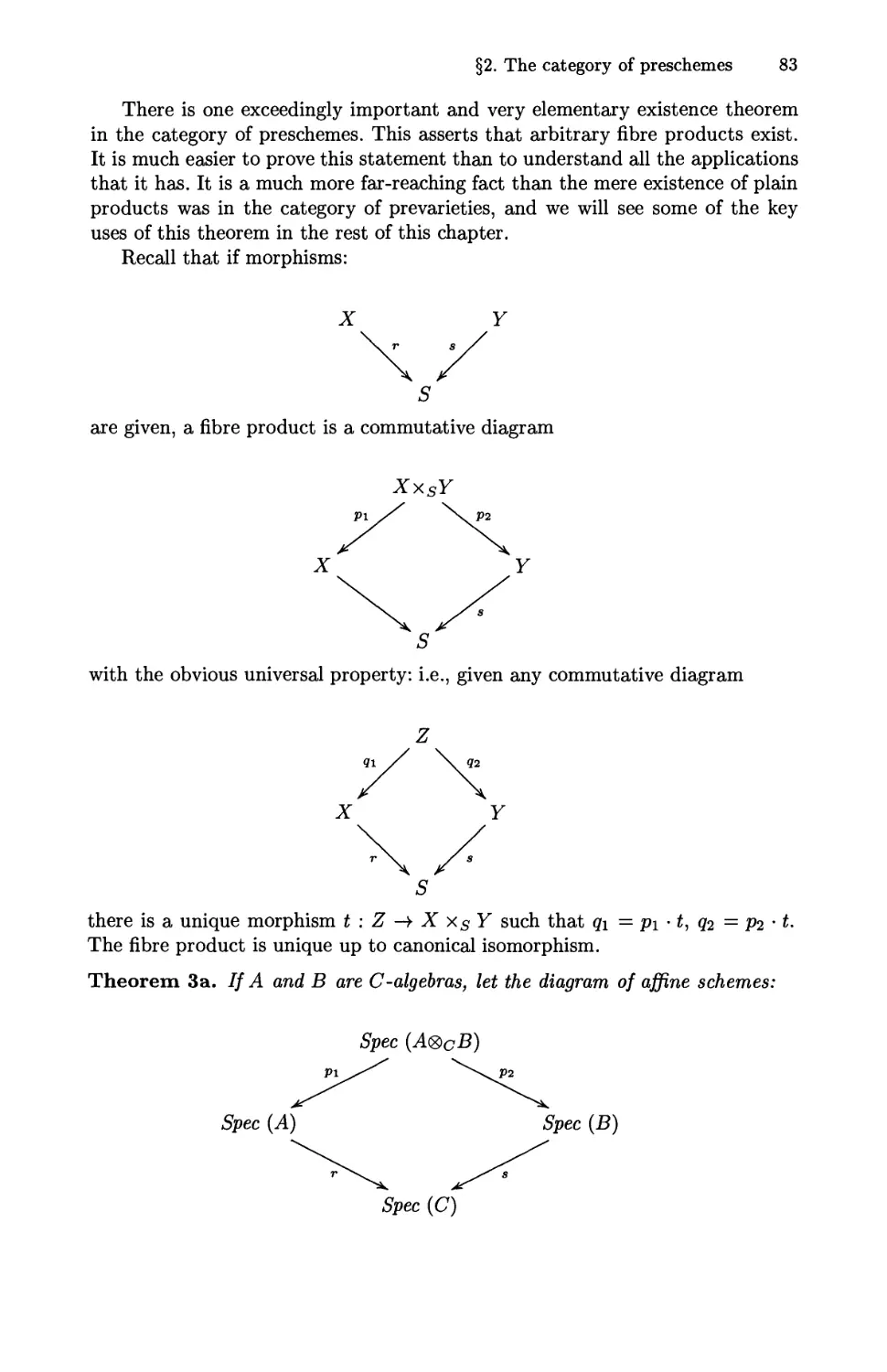
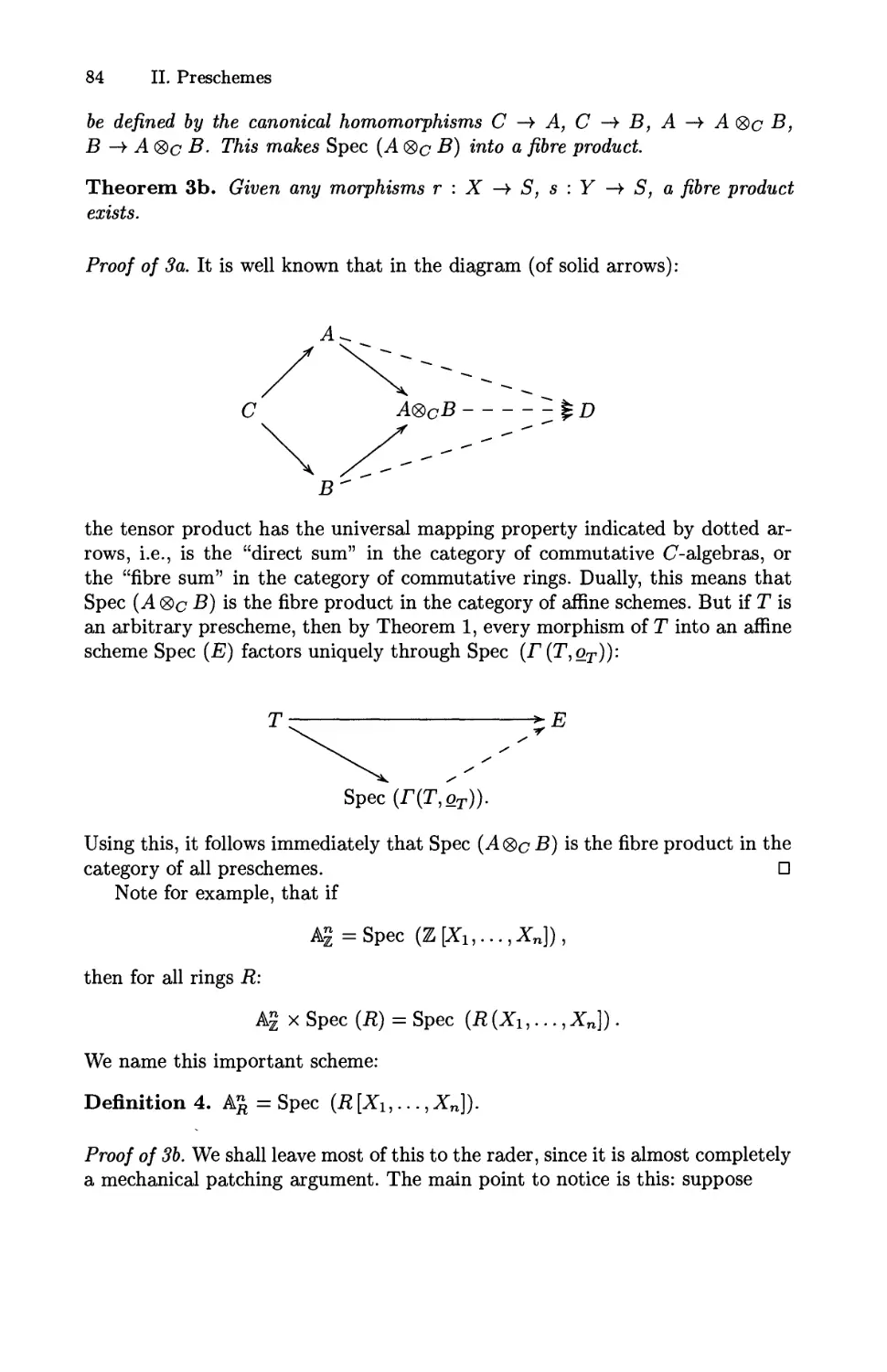
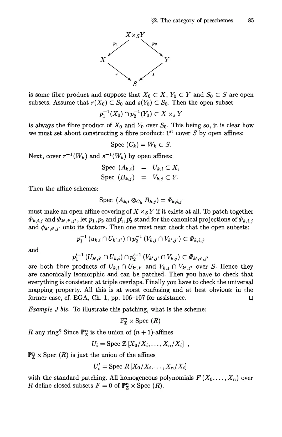
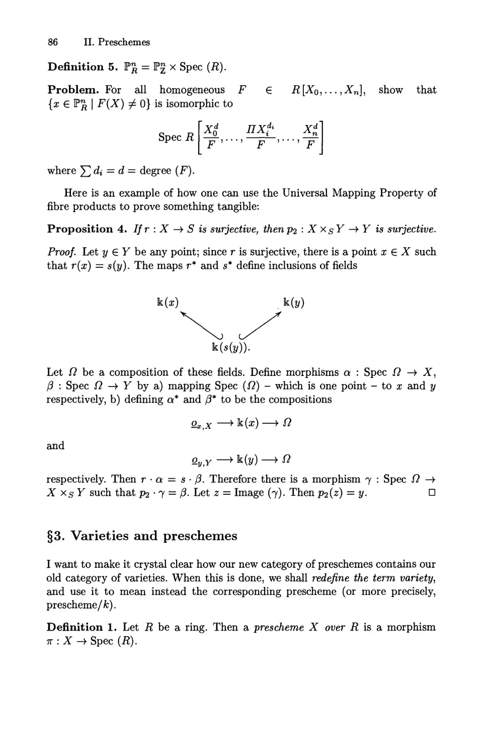
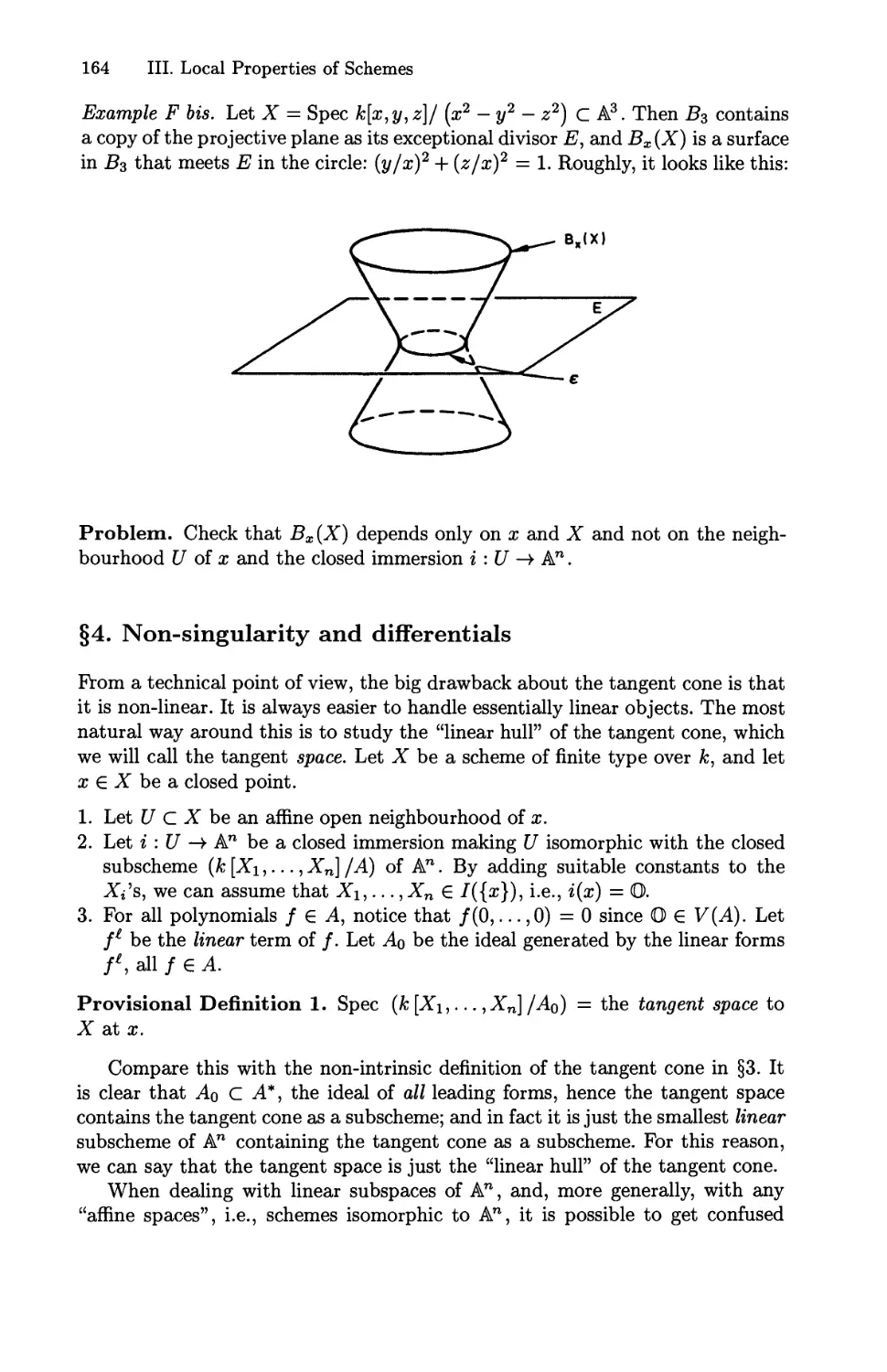
Текст
Lecture Notes in Mathematics 1358
Edilois:
A. Dokl. Heidelberg
F. Takcns, Groningcri
B. Tcissicr, Paris
Springer
Berlin
Heidelberg
New York
Barcelona
Hong Kong
London,
Milan
Paris
Singapore
Tokyo
David Mumford
The Red Book
of Varieties and Schemes
Second, Expanded Edition
Tnciudes the Michigan Lectures A974)
on Curves and their Jacobians
Springer
Authors
David В. Mumibrd
Division of Applied Mathematics, Box F
Brown University
Providence, RI 02912, USA
E-mail: David_Mumford(E?bro\vn edu
Enrico Arbarelio
Scuola Normale Superiore
7, Piazza dei Cavalieri
56126 Pisa, Italy
E-mail: ea@bibsns.sns.it
Cataloging-in-Pubiication Data applied for
Die Deutsche Bibliothck - CIP-Einheitsaufnahme
Mumford, David:
Tlie red book of varieties and schemes : includes the Michigan
lectures A974) on curves and their Jacobians / David Mumford. - 2.,
expanded ed. - Berlin ; Heidelberg ; New York ; Barcelona ; Hong
Kong ; London ; Milan ; Paris ; Singapore ; Tokyo : Springer, 1999
(Lecture notes in mathematics ; 1358)
ISBN 3-540-63293-X
Mathematics Subject Classification A991): 14-01, 14A15, !4НЮ. 14Н42, 141145
ISSN 0075-8434
ISBN 3-540-63293-X Springer-Vcrlag Berlin Heidelberg New York
This work is subject to copyright. All rights are reserved, whether the whole or part
of the material is concerned, specifically the rights of translation, reprinting, re-use
of illustrations, recitation, broadcasting, reproduction on microfilms or in any other
way, and storage in data banks. Duplication of this publication or pans thereof is
permitted only under the provisions of the Geiman Copyright Law of September 9,
1965. in its current version, and permission for use must always he obtained from
Springer-Vcrlag. Violations are liable for prosecution under the German Copyright
Law.
© Springer-Verlag Berlin Heidelberg 1999
Printed in Germany
The use of general descriptive' names, registered names, trademarks, etc. in this
publication does not imply, even in the absence of a specific statement, that such
names are exempt from the relevani protective laws and regulations and therefore
free for general use.
Typesetting: 1. Jcbram using a Springcr-TgX macro-package
SPIN: 10568814 41/3143-543210 - Printed on acid-free paper
Preface to the Second Edition
At the same time that the first edition of the Springer Lecture Notes version of
the "Red Book of Varieties and Schemes" was sold out, the supply of my lecture
notes "Curves and their Jacobians", published by the University of Michigan
Press, was also exhausted and the copyright returned to me. These two sets of
notes have similar purposes. At one time, I had had ambitious plans to write
a multi-volume introduction to algebraic geometry and specifically to moduli
problems, this being the part of the field which I knew best. Before writing
these, I gave lectures on various occasions to explain the ideas informally with
the idea that these might be a first draft for parts of a longer more polished
version. What I found, however, was that these first drafts, written informally,
with pictures and diagrams, printed in a typewriter font and, above all, being
short, were more appealing to many readers than a full-blown Grundlehrcn-style
book. Therefore, Springer-Verlag and I made the plan to keep both sets of notes
in print a bit longer, reprinting them together, with the original "Red Book" as
part one and "Curves and their Jacobians" as part two.
The "Red Book" originated in mimeographed lectures delivered at Harvard in
the 60's, whose primary goal was to show that the language of schemes was fun-
fundamentally geometric and expresses the intuitions of algebraic geometry clearly.
1 "Curves and their Jacobians", on the other hand, is a write-up of four lectures
given at the University of Michigan in 1974, whose goal was to give a bird's eye
view of curves, their moduli spaces, their jarobians and how these relate to each
othci. Although the styles differ because the "Red Book" was addressed to stu-
students and "Curves and their Jacobians" to faculty as well, both try to describe
ideas as informally and simply as possible.
Since my research now is in stochastic methods in signal processing and
image analysis (which I like to call "Pattern Theory" following Grenander), I
have not kept up with the literature on the1 moduli of curves. The last section of
the uriginal notes entitled "Guide to the Literature and References" is quite out
of date and it is impossible for me to bring it up to date, although I have added
reference.s to Harris' work with me and Eisenbud on the Kodaira dimension uf
the Moduli Space.
1 (Added in proof) Rereading Chapter 3, I reali' e that I particularly wished to show
that Zariski's work, on which I had grown up, could be recast, with no loss of its
force, in the language of schemes.
VI Preface to the Second Edition
For the Schottky problem, there has been a great deal of progress and Profes-
Professor Enrico Arbarello has generously contributed a new section "Supplementary
Bibliography on the Schottky Problem" to give pointers to this work. Another
useful reference for recent work is the book "The Moduli Space of Curves",
edited by Dijkgraaf, Faber and van dcr Geer, Birkhauscr-Boston.
Cambridge, Mass.
May, 1999. David Mumford
Preface to the First Edition
These notes originated in several classes that I taught in the mid 60's to intro-
introduce graduate students to algebraic geometry. I had intended to write a book,
entitled "Introduction to Algebraic Geometry", based on these courses and, as
a first step, began writing class notes. The class notes first grew into the present
three chapters. As there was a demand for them, the Harvard mathematics de-
department typed them up and distributed them for a while (this being in the dark
ages before Springer Lecture Kotos came to fill this need). They were called "In-
"Introduction to Algebraic Geometry: -preliminary version of the first 3 chapter^
and were bound in red. The intent was to write a much more inclusive book,
but as the years progressed, my ideas of what to include in this book changed.
The book became two volumes, and eventually, with almost no overlap with
these notes, the first volume appeared in 1976, entitled "Algebraic Geometry I:
complex protective varieties". The present plan is to publish shortly the second
volume, entitled "Algebraic Geometry II: schemes and cohomology", in collabo-
collaboration with David Eisenbud and Joe Harris.
David Gieseker and several others have, however, convinced me to let
Springer Lecture Notes reprint the original notes, long out of print, on the
grounds that they serve a quite distinct purpose. Whereas the longer book "Al-
"Algebraic Geometry" is a systematic and fairly comprehensive exposition of the
basic results in the field, these old notes had been intended only to explain in
a quick and informal way what varieties and schemes are, and give a few key
examples illustrating their simplest properties. The hope was to make the basic
objects of algebraic geometry as familiar to the reader as the basic objects of
differential geometry and topology: to make a variety as familiar as a manifold
or a simplicial complex. This volume is a reprint of the old notes without change,
except that the title has been changed to clarify their aim.
The weakness of these notes is what had originally driven me to undertake
the bigger project: there is no real theorem in them! I felt it was hard to convince
people that algebraic geometry was a great and glorious field unless you offered
them a theorem for their money, and that takes a much longer book. But for
a puzzled non-algebraic geometer who wishes to find the facts needed to make
sense of some algebro-gcomctric statement that they want to applv, these notes
may be a convenient way to learn quickly the basic definitions. In twenty years
of giving colloquium talks about algebraic geometry to audiences of mostly non-
VIII Preface to the First Edition
algebraic geometers, I have learned only too well that algebraic geometry is not
so easily accessible, nor are its basic definitions universally known.
It may be of some interest to recall how hard it was for algebraic geome-
geometers, even knowing the phenomena of the field very well, to find a satisfactory
language in which to communicate to each other. At the time these notes were
written, the field was just emerging from a twenty-year period in which every
researcher used his own definitions and terminology, in which the "foundations"
of the subject had been described in at least half a dozen different mathematical
"languages". Classical style researchers wrote in the informal geometric style of
the ftalian school, Weil had introduced the concept of specialization and made
this the cornerstone of his language and Zariski developed a hybrid of algebra
and geometry with valuations, universal domains and generic points relative
to various fields к playing important roles. But there was a. general realization
that not all the key phenomena could be clearly expressed and a frustration at
sacrificing the suggestive geometric terminology of the previous generation.
Then Grothendieck came along and turned a confused world of researchers
upside down, overwhelming them with the new terminology of schemes as well as
with a huge production of new and very exciting results. These notes attempted
to show something that was still very controversial at that time: that schemes
really were the most natural language for algebraic geometry and "that you did
not need to sacrifice geometric intuition when you spoke "scheme". I think this
thesis is now widely accepted within the community of algebraic geometry, and I
hope that eventually schemes will take their place alongside concepts like Banach
spaces and cohomology, i.e. as concepts which were once esoteric and abstruse,
but became later an accepted part of the kit of the working mathematician.
Grothendieck being sixty this year, it is a great pleasure to dedicate those notes
to him and to send him the message that his ideas remain the framework on
which subsequent generations will build.
Cambridge, Mass.
Feb. 21, 1988.
Table of Contents
Preface to the Second Edition V
Preface to the First Edition VII
Table of Contents IX
I. Varieties 1
§1. Some algebra, 1
§2. Irreducible algebraic sets 5
§3. Definition of a morphism 11
§4. Sheaves and affine varieties 16
§5. Definition of prevaricties and morphisins 25
§6. Products and tho Hausdorff Axiom 33
§7. Dimension 40
§8. The fibres of a morphism 48
§9. Complete varieties 54
§ 10. Complex varieties 57
II. Preschemes 65
§1. Spec (R) 6G
§2. The category of preschemes 77
§3. Varieties and preschemes 86
§4. Fields of definition 94
§5. Closed subprrachemes 103
§6. The functor of points of a prescheme 112
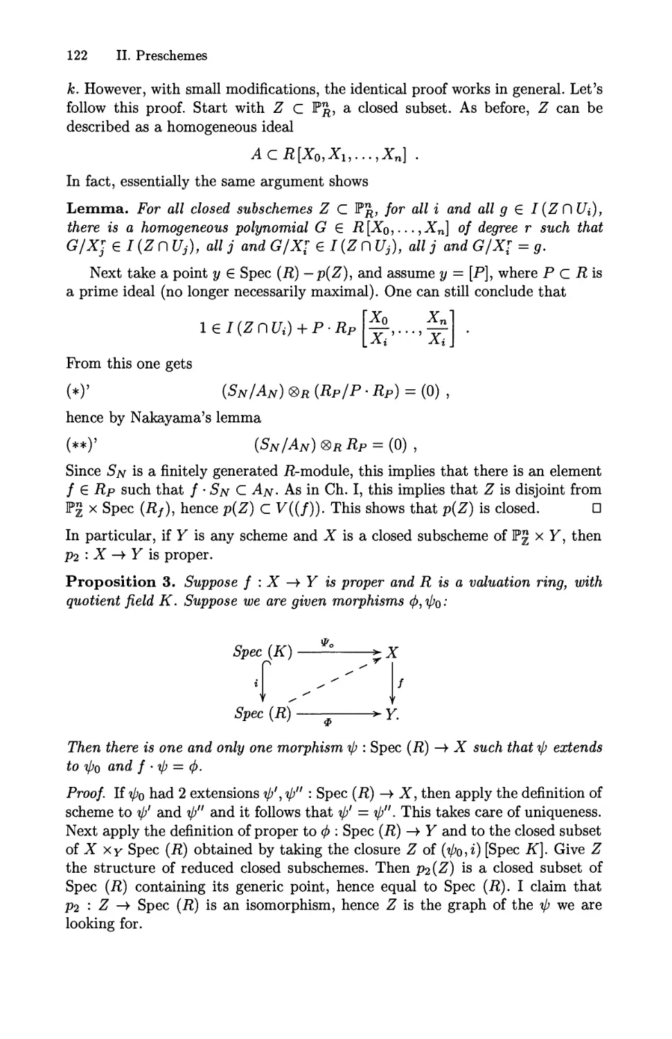
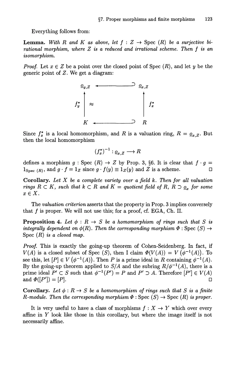
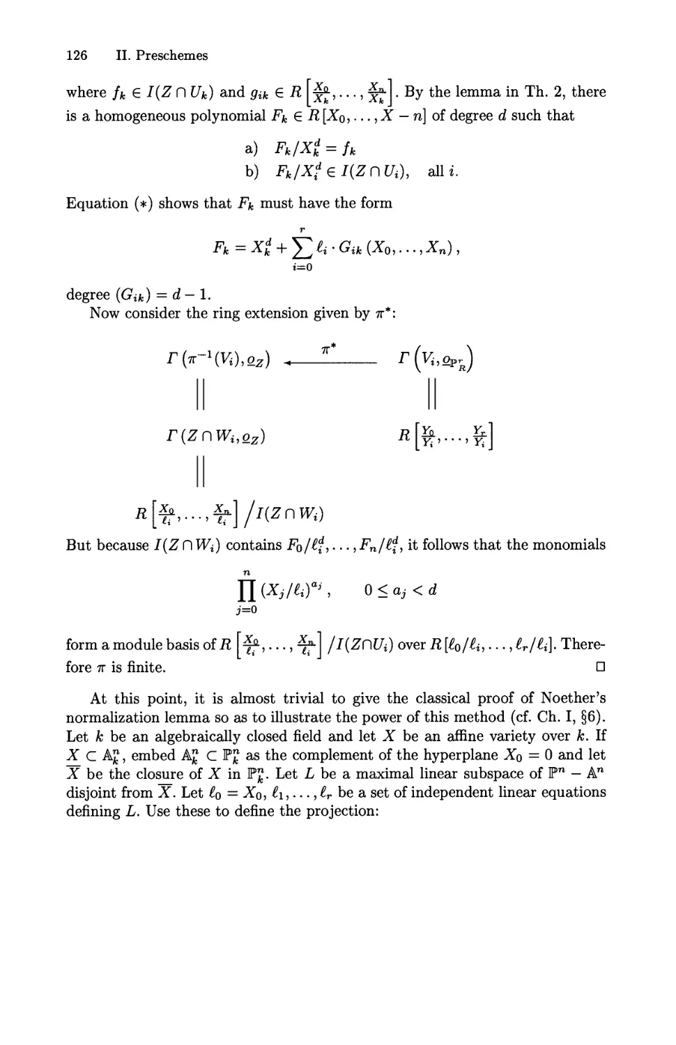
§7. Proper morphisms and finite morphisms 121
§8. Specialization 127
III. Local Properties of Schemes 137
§1. Quasi-coherent, modules 138
§2. Coherent modules 146
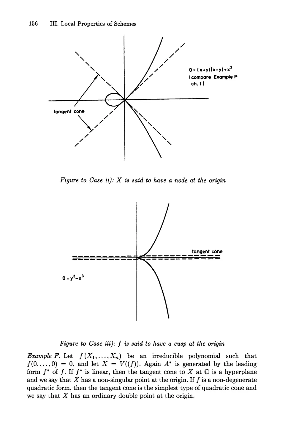
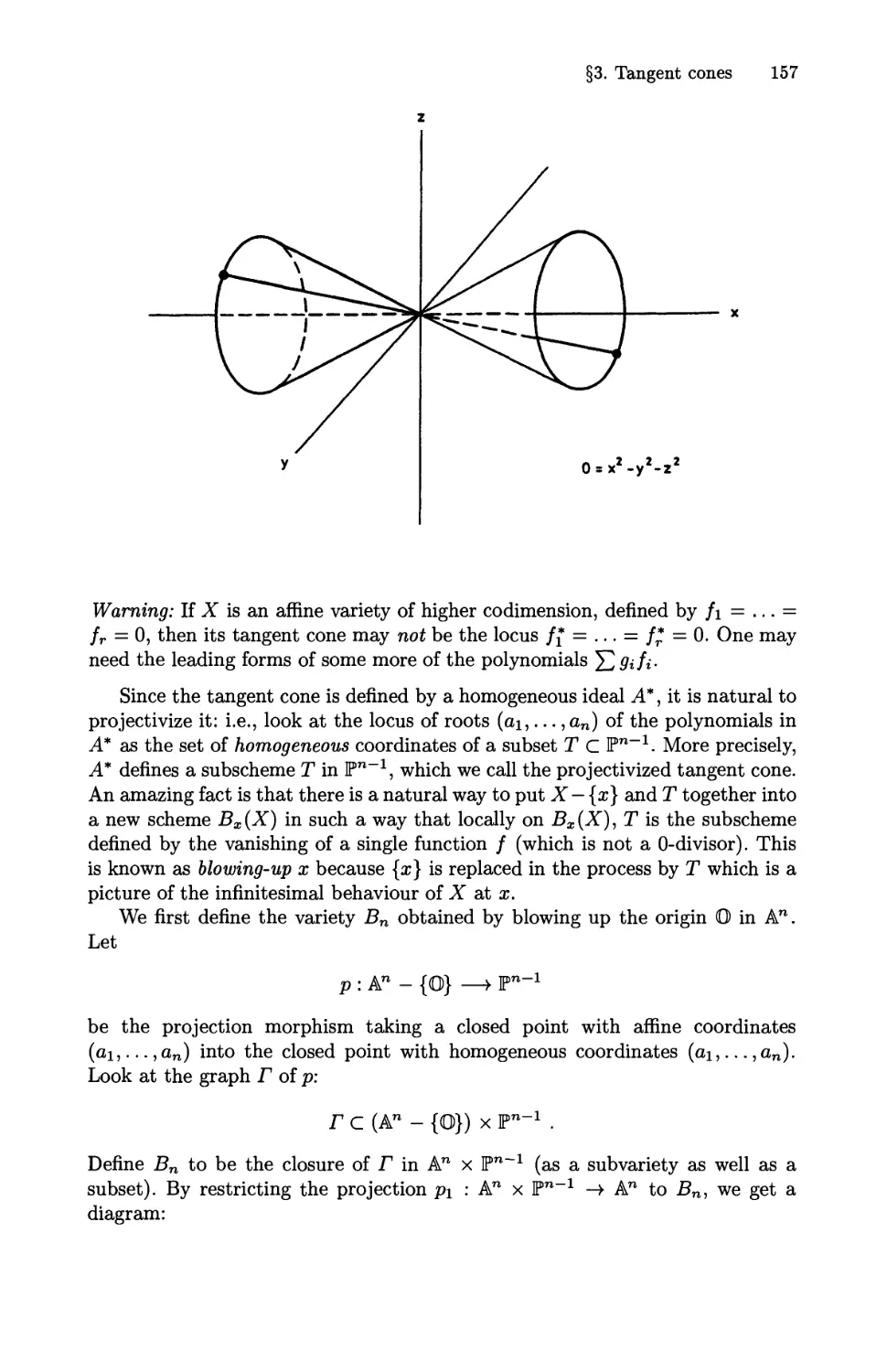
§3. Tangent cones 153
§4. Non-singularity and differentials 164
§5. Etale morphisms 174
§6. Unifonwing parameters 183
X Table of Contents
§7. Non-singularity and the UFD property 187
§8. Normal varieties and normalization 196
§9. Zariski's Main Theorem 207
§10. Flat and smooth morphisms 214
Appendix: Curves and Their Jacobians 225
Lecture I: What is a Curve and How Explicitly
Can We Describe Them? 229
Lecture II: The Moduli Space of Curves: Definition, Coordinatization,
and Some Properties 243
Lecture III: How Jacobians and Thota Functions Arise 257
Lecture IV: The Torelli Theorem and the Schottky Problem 271
Survey of Work on the Schottky Problem up to 199G
by Enrico Arbarello 287
References: The Red Book of Varieties and Schemes 293
Guide to the Literature and References:
Curves and Their Jacobians 294
Supplementary Bibliography on the Schottky Problem
by Enrico Arbarello 301
I. Varieties
The basic object of study in algebraic geometry is an arbitrary prescheme. How-
However, among all preschemes, the classical ones known as varieties are by far the
most accessible to intuition. Moreover, in dealing with varieties one can carry
over without any great difficulty the elementary methods and results of the
other geometric categories, i.e., of topological spaces, differentiable manifolds or
of analytic spaces. Finally, in any study of general preschemes, the varieties are
bound, for many reasons which I will not discuss here, to play a unique and cen-
central role. Therefore it is useful and helpful to have a basic idea of what a variety
is before plunging into the general theory of preschemes. We will fix through-
throughout an algebraically closed ground field к which will never vary. We shall restrict
ourselves to the purely geometric operations on varieties in keeping with the aim
of establishing an intuitive and geometric background: thus we will not discuss
specialization, nor will we use generic points. This set-up is the one pioneered by
Serre in his famous paper "Faisceaux algebriques coherents". There is no doubt
that it is completely adequate for the discussion of nearly all purely geometric
questions in algebraic geometry.
§1. Some algebra
We want to study the locus V of roots of a finite set of polynomials
fi (X\,..., Xn) in kn (k being an algebraically closed field). However, the basic
tool in this study is the ring of functions from V to к obtained by restricting
polynomials from kn to V. And we cannot get very far without knowing some-
something about the algebra of such a ring. The purpose of this section is to prove 2
basic theorems from commutative algebra that are key tools in analyzing these
rings, and hence also the loci such as V. We include these results because of
their geometric meaning, which will emerge gradually in this chapter (cf. §7).
On the other hand, we assume known the following topics in algebra:
1) The essentials of field theory (Galois theory, separability, transcendence de-
degree).
2) Localization of a ring, the behaviour of ideals in localization, the concept of
a local ring.
3) Noetherian rings, and the decomposition theorem of ideals in these rings.
4) The concept of integral dependence, (cf., for example, Zariski-Samuel, vol. 1).
D. Mumford: LNM 1358, pp. 1-63, 1999.
© Springer-Verlag Berlin Heidelberg 1999
2 I. Varieties
The first theorem is:
Noether's Normalization Lemma. Let R be an integral domain, finitely
generated over a field k. If R has transcendence degree n over k, then there
exist elements x\,..., xn € R, algebraically independent over k, such that R is
integrally dependent on the subring k[xi,... ,xn] generated by the x's.
Proof (Nagata). Since R is finitely generated over k, we can write R as a quo-
quotient:
R = k[Y1,...,Ym]/P ,
for some prime ideal P. If m = n, then the images yi,...,ym of the V's in
R must be algebraically independent themselves. Then P = @), and if we let
Xi = ?/i, the lemma follows. If m > n, we prove the theorem by induction on
m. It will suffice to find a subring S in R generated by m — 1 elements and
such that R is integrally dependent on S. For, by induction, we know that S
has a subring k[xi,...,xn] generated by n independent elements over which
it is integrally dependent; by the transitivity of integral dependence, R is also
integrally dependent on k[x\,...,xn] and the lemma is true for R.
Now the m generators y\,..., ym of R cannot be algebraically independent
over к since m > n. Let
/B/l,---,2/m) =0
by some non-zero algebraic relation among them (i.e., / (yi,..., ym) is a non-zero
polynomial in P). Let ri,... ,rm be positive integers, and let
Z2 = 2/2 - y{2 , Z3=y3-yl3,...,Zm=ym- J/[m •
Then
/B/i,32 +y[2,...,zm +y[m) = 0 ,
i.e., yi,Z2,...,zm are roots of the polynomial / (Yi, Z2 + Y{2 ,...,Zm + Y{m).
Each term a • YI y^ in / gives rise to various terms in this new polynomial,
i=l
including one monomial term
„ „,bi+r2b2 + ...+rmbm
a' V\
A moment's reflection will convince the reader that if we pick the n's to be large
enough, and increasing rapidly enough:
o«cr2 «;r3«: ...«;rm,
then these new terms a • Y^l+'"+Tmbm will all have distinct degrees, and one of
them will emerge as the term of highest order in this new polynomial. Therefore,
/ (YUZ2 +Y1r2,...,Zm + Y1r™)=b- Y? + [ terms of degree < N] ,
(b ф 0). This implies that the equation / {y\, z2 + y[2,. • •, zm + y[m) = 0 is an
equation of integral dependence for y\ over the ring k[z2,... ,2m]. Thus y\ is
integrally dependent on k[z2,.. .,zm], so y2,... ,ym are too since yi = Z{ + y7^
(i = 2,..., m). Therefore the whole ring R is integrally dependent on the subring
S = к [z2,..., zm]. By induction, this proves the lemma. □
§1. Some algebra 3
The second important theorem is:
Going-up theorem of Cohen-Seidenberg. Let R be a ring (commutative as
always) and S С R a subring such that R is integrally dependent on S. For all
prime ideals P С S, there exist prime ideals P' С R such that P' П S = P.
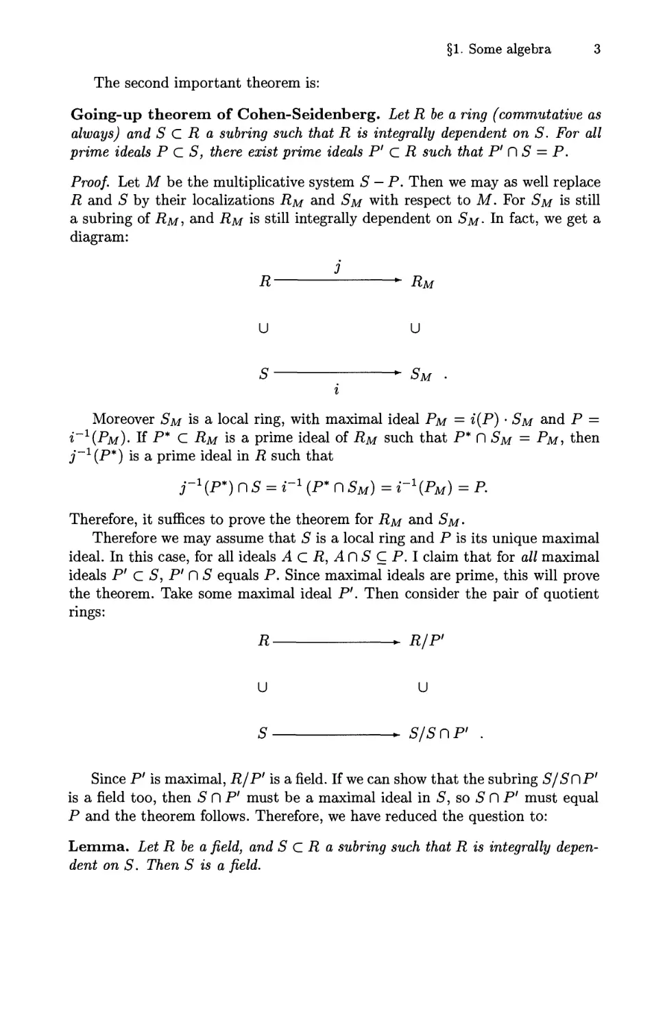
Proof. Let M be the multiplicative system S — P. Then we may as well replace
R and S by their localizations Rm and Sm with respect to M. For Sm is still
a subring of Rm, and Rm is still integrally dependent on Sm- In fact, we get a
diagram:
3
R RM
U U
S SM •
i
Moreover Sm is a local ring, with maximal ideal Рм = i(P) • Sm and P =
ъ~1{Рм)- If P* С Rm is a prime ideal of Rm such that P* П Sm = Рм, then
j~1{P*) is a prime ideal in R such that
Г1^*) ИЗ = Г1 (P*nSM) = г-г(Рм) = P
Therefore, it suffices to prove the theorem for Rm and Sm-
Therefore we may assume that S is a local ring and P is its unique maximal
ideal. In this case, for all ideals AcR, AnSCP.I claim that for all maximal
ideals P' С S, P' П S equals P. Since maximal ideals are prime, this will prove
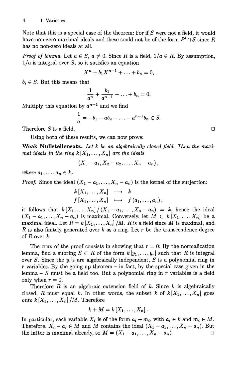
the theorem. Take some maximal ideal P'. Then consider the pair of quotient
rings:
R R/P'
U U
S S/SDP1 .
Since P' is maximal, R/P' is a field. If we can show that the subring S/SilP'
is a field too, then S П P' must be a maximal ideal in S, so S П P' must equal
P and the theorem follows. Therefore, we have reduced the question to:
Lemma. Let R be a field, and S С R a subring such that R is integrally depen-
dependent on S. Then S is a field.
4 I. Varieties
Note that this is a special case of the theorem: For if S were not a field, it would
have non-zero maximal ideals and these could not be of the form P' C\S since R
has no non-zero ideals at all.
Proof of lemma. Let a € S, а ф 0. Since R is a field, I/a € R. By assumption,
I/a is integral over S, so it satisfies an equation
I" + hXn-1 + ... + bn = 0,
bi € S. But this means that
Multiply this equation by an~1 and we find
- = -ъг - ab2 - ... - an~16n € S.
a
Therefore S is a field. □
Using both of these results, we can now prove:
Weak Nullstellensatz. Let к be an algebraically closed field. Then the maxi-
maximal ideals in the ring к [X\,..., Xn] are the ideals
(Xi - ai,X2 - a2,. ..,Xn- an),
where oi,... ,an € k.
Proof. Since the ideal {X\ — oi,... ,Xn — an) is the kernel of the surjection:
k[Xu...,Xn] —> к
it follows that к [X\,..., Xn] / {X\ — a\,..., Xn — an) = к, hence the ideal
(Xi — oi,... ,Xn — an) is maximal. Conversely, let M С к [Xi,... ,Xn] be a
maximal ideal. Let R = к [Xi,..., Xn] /M. R is a field since M is maximal, and
R is also finitely generated over A; as a ring. Let r be the transcendence degree
of R over к.
The crux of the proof consists in showing that r = 0: By the normalization
lemma, find a subring S С R of the form k[yi,...,yr] such that R is integral
over S. Since the y^s are algebraically independent, S is a polynomial ring in
r variables. By the going-up theorem - in fact, by the special case given in the
lemma - S must be a field too. But a polynomial ring in r variables is a field
only when r = 0.
Therefore R is an algebraic extension field of к. Since к is algebraically
closed, R must equal к. In other words, the subset к of k[Xi,...,Xn] goes
onto к [Xi,..., Xn] /M. Therefore
In particular, each variable Xi is of the form ai+rrii, with аг- € к and mi € M.
Therefore, Xi — o, € M and M contains the ideal (Xi — ai,..., Xn — an). But
the latter is maximal already, so M = (Xi — ai,..., Xn — an). О
§2. Irreducible algebraic sets 5
The great importance of this result is that it gives us a way to translate affine
space kn into pure algebra. We have a bijection between kn, on the one hand,
and the set of maximal ideals in k[Xi,...,Xn] on the other hand. This is the
origin of the connection between algebra and geometry that gives rise to our
whole subject.
§2. Irreducible algebraic sets
For the rest of this chapter к will denote a fixed algebraically closed field, known
as the ground field.
Definition 1. A closed algebraic subset of kn is a set consisting of all roots of
a finite collection of polynomial equations: i.e.,
{(xi,...,xn) | /i (xi,...,xn) = ■■• = fm(xi,...,xn) = 0} .
It is clear that the above set depends only on the ideal A = (Д,..., /m) generated
by the /j's in [X\,... ,Xn] and not on the actual polynomials /,. Therefore, if
A is any ideal in к [Xi,..., Xn], we define
V(A) = {xekn\ f(x) = 0 for all / € A} .
Since к [Xi,..., Xm] is a noetherian ring, the subsets of kn of the form V(A) are
exactly the closed algebraic sets. On the other hand, if E is a closed algebraic
set, we define
= {/€ k[Xu...,Xn] \f(x)=0 for all x € £} .
Clearly I(U) is an ideal such that S = V(I(U)). The key result is:
Theorem 1 (Hilbert's Nullstellensatz).
Proof. It is clear that у/А С I(V(A)). The problem is to show the other inclu-
inclusion. Put concretely this means the following:
Let A = (fi,..., /m). If g £ к [Х\,..., Xn] satisfies:
{/i (oi,...,on) = ... = /TO(oi,---,On) = 0} => p(ai,...,an) = 0
then there is an integer £ and polynomials hi,..., hm such that
To prove this, introduce the ideal
В = A- k[Xu.. .,Xn,Xn+1} + A - g - Xn+1)
6 I. Varieties
in к [X\,..., -Xn+i]. There are 2 possibilities: either В is a proper ideal, or В =
к [Xi,..., -Xn+i]. In the first case, let M be a maximal ideal in к [Xi,..., Xn+i]
containing B. By the weak Nullstellensatz of §1,
M = (Xi —ai,...,Xn — an,Xn+1 - on+i)
for some elements a; € k. Since M is the kernel of the homomorphism:
к [Xi,..., Xn, Xn+i\ > к
f '—> f{ai,---,an+i),
В С М means that:
i) Л (ab...,an) = ... = fm(ai,...,an) = 0
and
ii) 1= g(a1,...,an) -an+1.
But by our assumptionon g, (i) implies that g (oi,..., an) = 0, and this contra-
contradicts (ii). We can only conclude that the ideal В would not have been a proper
ideal.
But then 1 € B. This means that there are polynomials hi,..., hm, hm+i €
к [Xi,..., -Xn+i] such that:
fi (X\, . . ■ , Xn)
— 2 ^*
+ A "~ 9 (-^1> • • • j-^n) " -Xn+l) *
Substituting g~x for Xn+i in this formula, we get:
Clearing denominators, this gives:
for some new polynomials h* € к [Xi,..., Xn], i.e., g € \/~A. П
Corollary. V and I set up a bijection between the set of closed algebraic subsets
of kn and the set of ideals А С к [Xi,..., Xn] such that A = \[~A.
This correspondence between algebraic sets and ideals is compatible with the
lattice structures:
i) А с В => V(A) D V(B)
ii) 27i С E2 => I (Hi) D
iii) 1
§2. Irreducible algebraic sets 7
iv) V(A f\B) = V(A) U V(B)
where A,B,Aa are ideals, Hi, H2 closed algebraic sets.
Proof. All are obvious except possibly (iv). But by (i), V(AnB) D V(A)\JV(B).
Conversely, if с $ V(A) U V(B), then there exist polynomials / € A and g € В
such that /(ж) ф 0, g(x) ф 0. But then / • g € An В and (/ • g){x) ф 0, hence
x(£V(Ar\B). О
Definition 2. A closed algebraic set is irreducible if it is not the union of two
strictly smaller closed algebraic sets. (We shall omit "closed" in referring to these
sets).
Recall that by the noetherian decomposition theorem, if А С к [Xi,..., Xn]
is an ideal such that A = yA, then A can be written in exactly one way as an
intersection of a finite set of prime ideals, none of which contains any other. And
a prime ideal is not the intersection of any two strictly bigger ideals. Therefore:
Proposition 2. In the bisection of the Corollary to Theorem 1, the irreducible
algebraic sets correspond exactly to the prime ideals of к [Xi,..., Xn]. Moreover,
every closed algebraic set H can be written in exactly one way as:
H = Hi U ... U Нк
where the Hi are irreducible sets and Hi <£ Hj if i ф j.
Definition 3. The Hi of Proposition 2 will be called the components of H.
In the early 19th century it was realized that for many reasons it was inade-
inadequate and misleading to consider only the above "affine" algebraic sets. Among
others, Poncelet realized that an immense simplification could be introduced
in many questions by considering "projective" algebraic sets (cf. Felix Klein,
Die Entwicklung der Mathematik, part I, pp. 80-82). Even to this day, there is
no doubt that projective algebraic sets play a central role in algebro-geometric
questions; therefore we shall define them as soon as possible.
Recall that, by definition, Tn(k) is the set of (n+l)-tuples (x0,..., xn) € kn+1
such that some Xi ф 0, modulo the equivalence relation
(xo,...,xn) ~ (axo,...,axn), aek*,
(where k* is the multiplicative group of non-zero elements of k). Then an (n +1)-
tuple (жо,Ж1,...,жп) is called a set of homogeneous coordinates for the point
associated to it. Pn(fc) can be covered by n + 1 subsets Uq,Ui, ... ,Un, where
Tj _ ( points represented by homogeneous 1
^ coordinates (xo,xi,... ,xn) with жг- ф 0 J
Each Ui is naturally isomorphic to kn under the map
I. Varieties
kn
( \ f X0 Xi Xn\ Xi ... Л
(xo,x1,...,xn) i—> I—,—,...,— I, I— omitted] .
\ Xi Xi Xi J \Xi J
The original motivation for introducing Tn{k) was to add to the affine space
kn = Uo the extra "points at infinity" fn(k) - Uo so as to bring out into the
open the mysterious things that went on at infinity.
Recall that to all subvectorspaces W С kn+1 one associates the set of points
P € Fn(fc) with homogeneous coordinates in W: the sets so obtained are called
the linear subspaces L of Pn(&)- If W has codimension 1, then we get a hy-
perplane. In particular, the points "at infinity" with respect to the affine piece
Ui form the hyperplane associated to the subvectorspace Xi = 0. Moreover, by
introducing a basis into W, the linear subspace L associated to W is naturally
isomorphic to Pr(&), (r = diml'F — 1). The linear subspaces are the simplest
examples of projective algebraic sets:
Definition 4. A closed algebraic set in Fn(fc) is a set consisting of all roots of
a finite collection of homogeneous polynomials /; € к [Xo,..., Xn], 1 < i < m.
This makes sense because if / is homogeneous, and (xo,..., xn), (axo,..., axn)
are 2 sets of homogeneous coordinates of the same point, then
f(xo,...,xn)=Q «=^ / (az0, • • •, ocxn) = 0.
We can now give a projective analog of the V, I correspondence used in
the affine case. We shall, of course, now use only homogeneous ideals А С
к [Хо,..., Xn]: i.e., ideals which, when they contain a polynomial /, also contain
the homogeneous components of /. Equivalently, homogeneous ideals are the ide-
ideals generated by a finite set of homogeneous polynomials. If Л is a homogeneous
ideal, define
^ (ж°' • • •'Жп) are homogeneous coordinates
of
If U С Fn(A;) is a closed algebraic set, then define
T,y\ _ { ideal generated by all homogeneous polynomials 1
^ \ that vanish identically on U J
Theorem 3. V and I set up a bijection between the set of closed algebraic sub-
subsets of¥n(k), and the set of all homogeneous ideals А С к[Хо, ■.. ,Xn], such
that A = \f~A except for the one ideal A = (Xo,..., Xn).
Proof. It is clear that if U is a closed algebraic set, then V(I(U)) = U. Therefore,
in any case, V and / set up a bijection between closed algebraic subsets of Tn(k)
and those homogeneous ideals A such that:
§2. Irreducible algebraic sets 9
These ideals certainly equal their own radical. Moreover, the empty set is
V ((Xo,..., Xn)), hence 1 € / (V ((Xo,..., Xn))); so (Xo, ...,Xn) does not sat-
satisfy (*) and must be excluded. Finally, let A be any other homogeneous ideal
which equals its own radical. Let V*(A) be the closed algebraic set correspond-
corresponding to A in the affine space kn+1 with coordinates Xo,... ,Xn. Then V*(A) is
invariant under the substitutions
(Xo,..., Xn) —> (aX0,..., aXn) ,
all a € k. Therefore, either
1) V*(A) is empty,
2) V*(A) equals the origin only, or
3) V*(A) is a union of lines through the origin: i.e., it is the cone over the subset
V(A) in Pn(fc).
Moreover, by the affine Nullstellensatz, we know that
(**) A
In case 1), (**) implies that A = к [Xo,..., Xn], hence I(V(A)) - which always
contains A - must equal A since there is no bigger ideal. In case 2), (**) implies
that A = (Xo,... ,Xn) which we have excluded. In case 3), if / is a homoge-
homogeneous polynomial, then / vanishes on V(A) if and only if / vanishes on V*(A).
Therefore by (**), if / vanishes on V(A), then / € A, i.e.,
A D I(V(A)).
Since the other inclusion is obvious, Theorem 3 is proven. □
The same lattice-theoretic identities hold as in the affine case. Moreover, we
define irreducible algebraic sets exactly as in the affine case. And we obtain the
analog of Proposition 2:
Proposition 4. In the bijection of Theorem 3, the irreducible algebraic sets cor-
correspond exactly to the homogeneous prime ideals ( (Xo,..., Xn) being accepted).
Moreover, every closed algebraic set S in Tn(k) can be written in excatly one
way as:
S = Sx U ... U Sk ,
where the Si are irreducible algebraic sets and Si <]L Sj if 1ф j.
Problem. Let S С Tn(k) be a closed algebraic set, and let H be the hyperplane
Xo = 0. Identify Fn - H with kn in the usual way. Prove that S П (Pn - H)
is a closed algebraic subset of kn and show that the ideal of S П (Fn — H) is
derived from the ideal of S in a very natural way. For details on the relationship
between the affine and projective set-up and on everything discussed so far, read
Zariski-Samuel, vol. 2, Ch. 7, §§3,4,5 and 6.
10 I. Varieties
Example A. Hypersurfaces. Let / (Xo,... ,Xn) be an irreducible homogeneous
polynomial. Then the principal ideal (/) is prime, so / = 0 defines an irreducible
algebraic set in Fn(fc) called a hypersurface (e.g. plane curve, surface in 3-space,
etc.).
Example B. The twisted cubic in Рз(&). This example is given to show the exis-
existence of nontrivial examples: Start with the ideal:
Ao = (xz - y2,yw - z2) С k[x,y,z,w].
V(A0) is just the intersection in Тз(к) of the 2 quadrics xz = y2 and yw = z2.
Look in the affine space with coordinates
X = x/w, Y = y/w, Z = z/w
(the complement of w = 0). In here, V(A0) is the intersection of the ordinary
cone XZ = Y2, and of the cylinder over the parabola Y = Z2. This intersection
falls into 2 pieces: the line Y = Z = 0, and the twisted cubic itself. Correspond-
Correspondingly, the ideal Ao is an intersection of the ideal of the line and of the twisted
cubic:
Ao = (j/, z) П (xz - y2, yw - z2, xw - yz) .
The twisted cubic is, by definition, ^(^4). [To check that A is prime, the simplest
method is to verify that A is the kernel of the homomorphism ф:
k[x,y,z,w] -A k[s,t]
ф(х) = s3
ф(у) = s2t
ф{г) = st2
ф(т) = t3 ] .
In practice, it may be difficult to tell whether a given ideal is prime or whether
a given algebraic set is irreducible. It is relatively easy for principal ideals, i.e.,
for hypersurfaces, but harder for algebraic sets of higher codimension. A good
deal of effort used to be devoted to compiling lists of all types of irreducible
algebraic sets of given dimension and "degree" when these were small numbers.
In Semple and Roth, Algebraic Geometry, one can find the equivalent of such
lists. A study of these will give one a fair feeling for the menagerie of algebraic
sets that live in P3, F4 or F5 for example. As for the general theory, it is far from
definitive however.
§3. Definition of a morphism 11
§3. Definition of a morphism
We will certainly want to know when 2 algebraic sets are to be considered iso-
morphic. More generally, we will need to define not just the set of all algebraic
sets, but the category of algebraic sets (for simplicity, in Chapter 1, we will stick
to the irreducible ones).
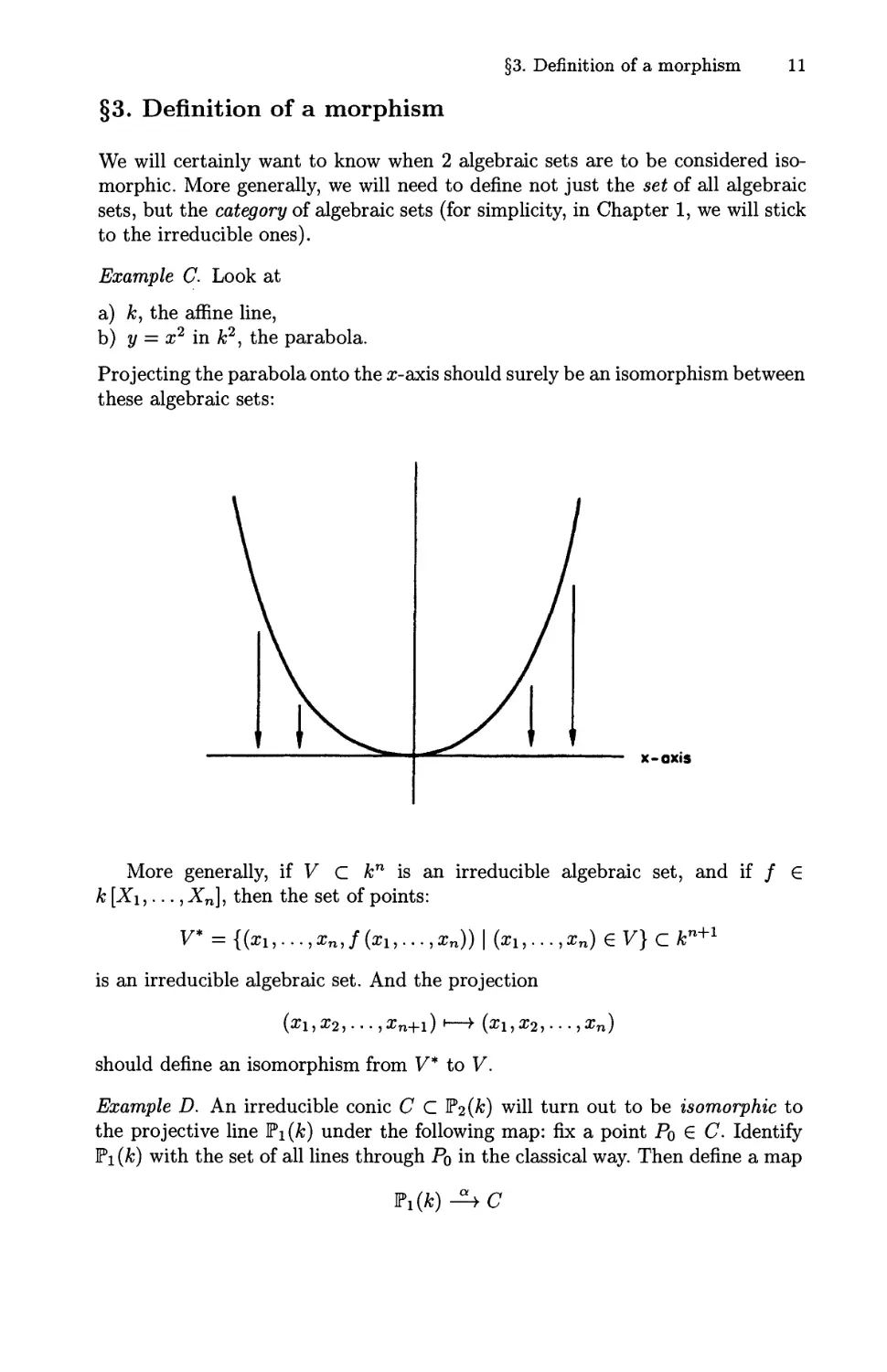
Example C. Look at
a) k, the affine line,
b) у = x1 in A;2, the parabola.
Projecting the parabola onto the x-axis should surely be an isomorphism between
these algebraic sets:
X-QXIS
More generally, if V С kn is an irreducible algebraic set, and if / G
к [Xi,..., Xn], then the set of points:
V* = {(x1,...,xn,f(x1,...,xn))\(xu...,xn)eV}ckn+l
is an irreducible algebraic set. And the projection
(xi,x2,... ,xn+i) i—> (xi,x2,.. -,xn)
should define an isomorphism from V* to V.
Example D. An irreducible conic С С Р2(&) will turn out to be isomorphic to
the projective line Pi(&) under the following map: fix a point Pq £ C. Identify
Pi (k) with the set of all lines through Po in the classical way. Then define a map
12 I. Varieties
by letting a(d) for all lines t through Po be the second point in which t meets
C, besides Po. Also, if t is the tangent line to С at Po, define a(t) to be Pq itself
(since Pq is a "double" intersection of С and this tangent line).
Example E. T\(k) and the twisted cubic Рз(&) will be isomorphic. For T\(k)
consists of the pairs (s,t) modulo (s,t) ~ (as,at), i.e., of the set of ratios
C = s/t including /3 = oo. Define a map
by a(C) = the point with homogeneous coordinates (l,/3,/32,/33) and a(oo) =
@,0,0,1).
The image points clearly satisfy xz = y2, yw = z2 and zw = yz, so they are
on the twisted cubic. The reader can readily check that a maps Pi (k) onto the
twisted cubic.
Example F. Let С be a cubic curve in Рг(А;) and let Po £ С For any point
P € C, let t be the line through P and Po and let a(P) be the third point
in which t meets C. Although this may not seem as obvious as the previous
examples, a will be an automorphism of С of order 2.
We shall use this example later to work out our definition in a nontrivial case.
Now turn to the problem of actually defining morphisms, and hence isomor-
isomorphisms, of irreducible algebraic sets. First consider the case of 2 irreducible affine
algebraic sets.
Definition 1. Let Sx С kni and E2 С кП2 be two irreducible algebraic sets. A
map
a : E\ —> £2
will be called a morphism if there exist n-2 polynomials /1,..., /П2 in the variables
Xi,..., Xni such that
(*) a(x) = (/i(xi,...,xni),...,/n2 (xi,...,xni))
for all points x = (xi,... ,xni) e E\.
§3. Definition of a morphism 13
Note one feature of this definition: it implies that every morphism a from E\ to
E2 is the restriction of a morphism a' from kni to km. This may look odd at
first, but it turns out to be reasonable - cf. §4. Note also that with this definition
the map in Example С above is an isomorphism, i.e., both it and its inverse are
morphisms.
To analyze the definition further, suppose
P1 С k[Xlt...,Xni]
P2 С *[Xi,...,Xna]
are the prime ideals I (Hi) and I{E2) respectively. Set
Then Ri (resp. R2) is just the ring of A;-valued functions on E\ (resp. E2)
obtained by restricting the ring of polynomial functions on the ambient affine
space. Suppose g £ R2. Regarding g as a function on E2, the definition of
morphism implies that the function g • a on E\ is in Ri - in fact
Therefore a induces a /г-homomorphism:
a* :R2 —> Ri.
Moreover, note that a is determined by a*. This is so because the polynomials
/1,..., fn2 can be recovered - up to an element of Pi - as a* (Xi),..., a* (Xn^)\
and the point a(x), for x e Ui, is determined via /i,.-.,/n2 modulo Pi
by equation (*). Even more is true. Suppose you start with an arbitrary k-
homomorphism
Л : R2 —У Ri •
Let /1 be a polynomial in к [X\,..., Xni] whose image modulo Pi equals X(Xi),
for all 1 < i < ni. Then define a map
by
a' (xi,..., xni) = (/1 (xi,..., xni),..., /n2 (xi,..., xni)).
If x = (xi,...,xni) e Hi, then actually a'(x) will be in E2'- for if g € P2, then
g(a\x))=g(f1(x),...,fna(x)).
But g (fu ..., /na) =g(X (Xi),..., Л (Xna)) modulo Pi
= X(g) modulo Pi
= 0 modulo Pi .
Therefore, g(a'(x)) = 0 and a'(x) e E2.
We can summarize this discussion in the following:
14 I. Varieties
Definition 2. Let E С kn be an irreducible algebraic set. Then the affine
ring Г(Е) is the ring of /г-valued functions on E given by polynomials in the
coordinates, i.e.,
k[Xu...,Xn}/I(E).
Proposition 1. If Ei, Ei are two irreducible algebraic sets, then the set ofmor-
phisms from E\ to Ei and the set of k-homomorphisms from Г(Е2) to Г(Е\)
are canonically isomorphic:
hom(E1,E2) *< honifc (Г(Е2),Г(Е1)).
Corollary. // E is an irreducible algebraic set, then Г{Е) is canonically iso-
isomorphic to the set of morphisms from E to k.
Proof. Note that Г (к) is just k[X].
Using Г(Е), we can define a subset V(A) of E for any ideal А С Г(Е) as
{x e E | f(x) = 0 for all f eA}.
Moreover, the Nullstellensatz for kn implies immediately the Nullstellensatz for
E:
{/ e Г(Е) I f(x) = 0 for all x e V(A)} = VI.
Even more than Proposition 1 is true:
Proposition 2. The assignment
E h—► Г(Е)
extends to a contravariant functor Г:
Category of irreducible
algebraic sets + morphisms
}j Category of finitely generated integral 1
| domains over к + k-homomorphisms j
which is an equivalence of categories.
Proof Prop. 1 asserts that Г is a fully faithful functor. The other fact to check
is that every finitely generated integral domain R over к occurs as Г(Е). But
every such domain can be represented as:
hence as Г(Е) where E is the locus of zeroes of /i,..., /TO in kn. D
Because of the usefulness of continuity in topology and other parts of geome-
geometry, another natural question is whether there is a natural topology on irreducible
algebraic sets in which all morphisms are continuous. We will certainly want
points of к to be closed, so their inverse images by morphisms must be closed.
If we take the weakest topology satisfying this condition, we get the following:
§3. Definition of a morphism 15
Definition 3. A closed set in kn is to be a closed algebraic set V(A). By the
results of §2, these define a topology in kn, called the Zariski topology. An ir-
irreducible algebraic set E С кп is given the induced topology, again called the
Zariski topology. It is clear that the closed sets of E are exactly the sets V(A),
where A is an ideal in Г(Е).
It is easy to check that all morphisms are continuous in the Zariski topology.
A basis for the open sets in the Zariski topology on E is given by the open sets:
Ef = {x e E | f{x) ф 0}
for elements / £ ГA7). In fact, Ef = E — F((/)), hence Ef is open. And if
U = E — ViA) is an arbitrary open set, then
U=
/ел
One should notice that the Zariski topology is very weak. On к itself, for
instance, it is just the topology of finite sets, the weakest T\ topology (since any
ideal A in k[X] is principal - A = if) - therefore ViA) is just the finite set
of roots of /). It follows that any bijection a : к —> к is continuous, so not all
continuous maps are morphisms. In any case this is a very unclassical type of
topological space.
Definition 4. A topological space X is noetherian if its closed sets satisfy the
descending chain condition (d.c.c). It is equivalent to require that all open sets be
quasi-compact (= having the Heine-Borel covering property, but not necessarily
T2).
Now since ideals in к [X\,..., X2] satisfy the a.c.c, it follows that closed sets
satisfy the d.c.c. - so the Zariski topology is noetherian.
Our simple definition of morphisms for affine algebraic sets does not work
for projective algebraic sets. The trouble is that it automatically implied that
the morphism will extend to a morphism of the ambient affine space. There is
no analogous fact in the projective case. Look at the case of Example D. Let E\
be the conic with homogeneous equation
(*) xz = y2
in P2(fc). Let E2 = Pi(fc). Let Po e Ex be the point @,0,1). To every point
Q £ Рг(^) — {Po}, we can associate the line PoQ, and by identifying the pencil
of lines through Po with Pi (A;) we get a point of Pi (A;). In terms of coordinates,
this can be expressed by the map:
(a, 6, c) 1—> (a, b)
as long as ia,b,c) are not homogeneous coordinates for Po, i.e., a or b is not
zero. Let (s,£) be homogeneous coordinates in Pi (A;). Then the map from E\ to
Ei should be defined by:
16 I. Varieties
s = x
Unfortunately, this is undefined at Po itself. But consider the second map defined
by:
s = У
t = z .
This is defined except at the point Pi £ E\ with coordinates A,0,0); moreover,
at points on E\ not equal to Pi or P2, the ratios (x : y) and (y : z) are equal in
view of the equation (*). Therefore A and В together define everywhere a map
from Ei to Ei. On the other hand, it will turn out that there are no surjective
morphisms at all from P2(fc) to Pi(fc) (cf. §7).
Thus defining morphisms between projective sets is more subtle. We find that
we must define morphisms locally and patch them together. But the problem
arises: on which local places. We could use the affine algebraic sets
Е-ЕПН
where H С Pn(&) is a hyperplane. But in general these will not be small enough.
We shall need arbitrarily small open sets in the Zariski-topology:
Definition 5. A closed setin Pn(&) is to be a closed algebraic set V(A). By the
results of §2, these define a topology in Pn(&), the Zariski-topology. Irreducible
algebraic sets themselves are again given the induced topology. As in the affine
case, a basis for the open sets is given by:
where / is a homogeneous polynomial. Moreover, it is clear that the Zariski
topology on fn(k) is noetherian.
Problem. Check that Tn(k)x0 is homeomorphic to kn under the usual map
i,.. .,xn/x0).
Finally, to define morphisms locally, we will need to attach affine coordinate
rings to a lot of the Zariski-open sets U and give a definition of affine morphism in
terms of local properties. Clearly, we should begin by constructing the apparatus
used for defining things locally.
§4. Sheaves and affine varieties
Definition 1. Let X be a topological space. A presheaf F on X consists of
i) for all open U С X, a set F(U)
ii) for all pairs of open sets Ui C^a map ("restriction")
vesU2Ul : F(U2) —
§4. Sheaves and affine varieties 17
such that the following axioms are satisfied:
b) IfUi CU2 CU3, then
F(U3)
F(U2)
commutes.
Definition 2. If Fi, F2 are presheaves on X, a map <p : F\ —> F2 is a collection
of maps (p(U) : Fi(l7) ->• F2(U) for each open C/" such that if 17 С V,
tp(V)
F2(V)
resv,u
resy,u
tp(U)
F2(U)
commutes.
Definition 3. A presheaf F is a sheaf if for every collection {£/,} of open sets
in X with U = UUi, the diagram
is exact, i.e., the map
JJ
is injective, and its image is the set on which
П
and
П resE/^nt/; : П F(uj) "^ П
П
agree.
18 I. Varieties
When we pull this high-flown terminology down to earth, it says this.
1) If xi,X2 £ F(U) and for all г, resu,Ui^i = Tesu,Ui^2, then xi = xi. (That is,
elements are uniquely determined by local data.)
2) If we have a collection of elements Xi £ F(Ui) such that res^^n [/,£;/ =
wsUj,Uir\UjXj for all г and j then there is an x £ F(U) such that res^^x = Xi
for all г. (That is, if we have local data which are compatible, they actually
"patch together" to form something in F(U).)
Example G. Let X and Y be topological spaces. For all open sets U С X,
let F(U) be the set of continuous maps U —> Y. This is a presheaf with the
restriction maps given by simply restricting maps to smaller sets; it is a sheaf
because a function is continuous on UUi if and only if its restrictions to each Ui
are continuous.
Example H. X and Y differentiable manifolds. F(U) = differentiable maps U —>•
Y. This again is a sheaf because differentiability is a local condition.
Example I. X, Y topological spaces, G(U) = continuous functions U —> Y which
have relatively compact image. This is a subpresheaf of the first example, but
clearly need not be a sheaf.
Example J. X a topological space, F(U) = the vector space of locally constant
real-valued functions on U, modulo the constant functions on U. This is clearly
a presheaf. But every s £ F(U) goes to zero in П F(Ui) for some covering {Ui},
while if U is not connected, F(U) ф @). Therefore it is not a sheaf.
Sheaves are almost standard nowadays, and we will not develop their prop-
properties in detail. Recall two important ideas:
A) Stalks. Let F be a sheaf on X, x £ X. The collection of F(U), U open
containing x, is an inverse system and we can form
Fx = Urn F(U) ,
xeu
called the stalk of F at x.
Example. Let F(U) = continuous functions U ->R. Then Fx is the set of germs
of continuous functions at x. It is Ux(zuF(U) modulo an equivalence relation:
/i ~ /2 if /1 and /2 agree in a neighbourhood of x.
B) Sheafification of a presheaf Let Fo be a presheaf on X. Then there is a sheaf
F and a map / : Fo —> F such that if g : Fo —> F' is any map with F' a sheaf,
there is a unique map h : F —>• F' such that
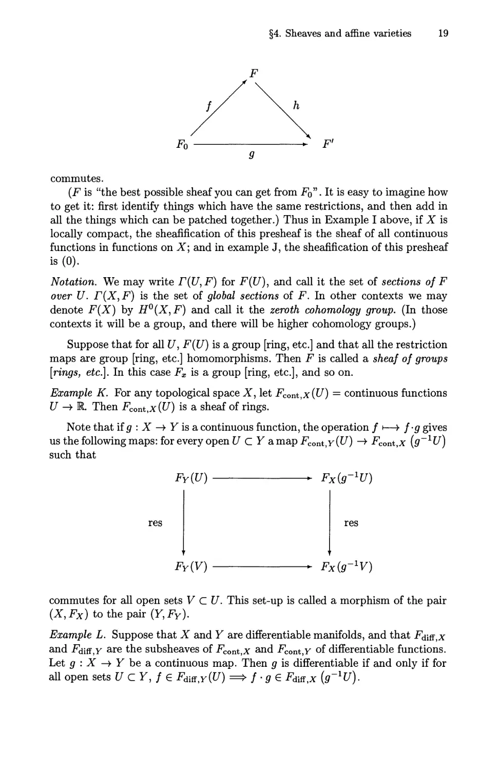
§4. Sheaves and affine varieties 19
F'
commutes.
(F is "the best possible sheaf you can get from Fo". It is easy to imagine how
to get it: first identify things which have the same restrictions, and then add in
all the things which can be patched together.) Thus in Example I above, if X is
locally compact, the sheafification of this presheaf is the sheaf of all continuous
functions in functions on X; and in example J, the sheafification of this presheaf
is @).
Notation. We may write F(U,F) for F(U), and call it the set of sections of F
over U. F(X, F) is the set of global sections of F. In other contexts we may
denote F(X) by H°(X,F) and call it the zeroth cohomology group. (In those
contexts it will be a group, and there will be higher cohomology groups.)
Suppose that for all U, F(U) is a group [ring, etc.] and that all the restriction
maps are group [ring, etc.] homomorphisms. Then F is called a sheaf of groups
[rings, etc]. In this case Fx is a group [ring, etc.], and so on.
Example K. For any topological space X, let Fcont,x(U) = continuous functions
£/"—>• E. Then Fcont,x(U) is a sheaf of rings.
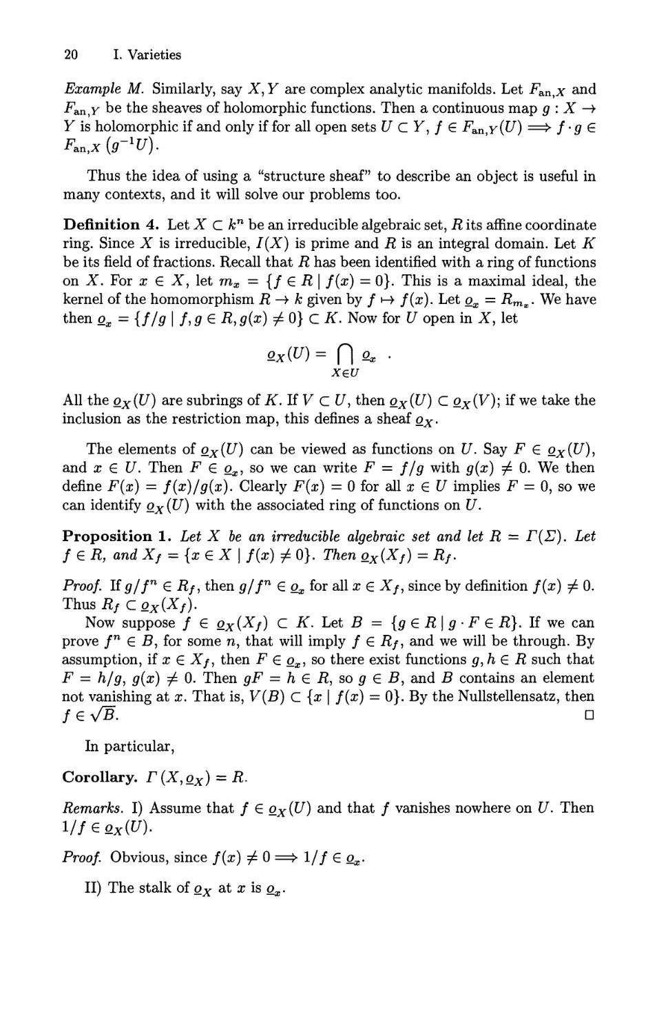
Note that if g : X —> Y is a continuous function, the operation / i—>■ f-g gives
us the following maps: for every open U С Y a map Fcont,y (U) ->• Fcont}x (g~XU)
such that
FY(U) ^ Fxig^U)
res
res
FY(V)
Fx(g-lv)
commutes for all open sets V С U. This set-up is called a morphism of the pair
(X,FX) to the pair (Y,FY).
Example L. Suppose that X and Y are differentiable manifolds, and that i*diff,x
and .Fdiff,y are the subsheaves of Fconttx and -Fcont,y of differentiable functions.
Let g : X —> Y be a continuous map. Then g is differentiable if and only if for
all open sets U CY, f e Fdiff}Y(U) => f .g e Fdiff)x (g^U).
20 I. Varieties
Example M. Similarly, say X, Y are complex analytic manifolds. Let F&ntx and
-Fan,у be the sheaves of holomorphic functions. Then a continuous map g : X —>
Y is holomorphic if and only if for all open sets U С Y, / £ Fan y(U) ==>■ f -g £
F^x^U).
Thus the idea of using a "structure sheaf" to describe an object is useful in
many contexts, and it will solve our problems too.
Definition 4. Let X С kn be an irreducible algebraic set, R its affine coordinate
ring. Since X is irreducible, I(X) is prime and R is an integral domain. Let К
be its field of fractions. Recall that R has been identified with a ring of functions
on X. For x £ X, let mx = {f £ R\ f(x) = 0}. This is a maximal ideal, the
kernel of the homomorphism R —> к given by / •->■ f(x). Let ox = Rmx. We have
then ox = {f/g \ f,g £ R,g(x) ф 0} С К. Now for U open in X, let
Ox(U) = П Д. •
xeu
All the QX(U) are subrings of K. If V С U, then ox(U) С ox(V); if we take the
inclusion as the restriction map, this defines a sheaf ox.
The elements of QX(U) can be viewed as functions on U. Say F £ ox(U),
and x £ U. Then F £ ox, so we can write F = f/g with g(x) ф 0. We then
define F(x) = f(x)/g(x). Clearly F(x) = 0 for all x £ U implies F = 0, so we
can identify ox(U) with the associated ring of functions on U.
Proposition 1. Let X be an irreducible algebraic set and let R = Г(£). Let
f £ R, and Xf = {x £ X | f(x) ф 0}. Then Qx(Xf) = Rf.
Proof. lig/fn £ Rf, then g/fn £ ox for all x £ Xf, since by definition f(x) ф 0.
Thus Rf Cox(Xf).
Now suppose / £ ox(Xf) С К. Let Б = {g £ R \ g ■ F £ R}. If we can
prove fn £ B, for some n, that will imply f £ Rf, and we will be through. By
assumption, if x £ Xf, then F £ ox, so there exist functions g,h £ R such that
F = h/g, g(x) ф 0. Then gF = h £ R, so g £ B, and В contains an element
not vanishing at x. That is, V(B) С {х \ f(x) = 0}. By the Nullstellensatz, then
feVB. a
In particular,
Corollary. Г(Х,ох) = R.
Remarks. I) Assume that / £ ox{U) and that / vanishes nowhere on U. Then
Proof. Obvious, since f(x) ф 0 ==> 1/f £ ox.
II) The stalk of ox at x is ox.
§4. Sheaves and affine varieties 21
Proof. Since the sets Xf are a basis of the Zariski topology of X, we have
lim ox{U) = lim ox{Xf) = lim Rf.
Since all restriction maps in our sheaf are injective, this is just \J Rf, which
/(*)#o
is clearly ox. D
III) The field К can also be recovered from the sheaf ox. Recall that X is
irreducible, i.e., not the union of two proper closed subsets. Equivalently, the
intersection of any two nonempty open sets is nonempty. But this means that
we actually have an inverse system of all open sets, just like our previous in-
inverse systems of open sets containing a given point x; in this way we can define
a generic stalk of any sheaf F on X. In particular, it is evident that К is the
generic stalk of the structure sheaf ox •
IV) If h £ 2X(U) for some open U С X, then it need not be true that
h = f/g with f,g (E R and g vanishing nowhere on U. For example, let X С к*
be V{xw — yz), and let U = Xy U Xw. The following function h € ox{U) is not
equal to f/g, g ф 0 in U: h = x/y on Xy, and h = z/w on X^2. The proposition
shows that this is true however if U has the form Xg.
Proposition 2. Let X С kn, Y С кт be irreducible algebraic sets, and let
f : X -> Y be a continuous map. The following conditions are equivalent:
i) f is a morphism
ii) forallger(Y,oY),g-fer(X,ox)
in) for all open U С Y, and g в Г (U,oY) =>• g • f e Г (f^U, ox)
iv) for all x e X, and g £ of^ => g ■f £ ox.
Proof. Trivially iii) => ii), and iv) ==> iii) by the definition of ox. i) 4=Ф ii) is
essentially proved in Proposition 1, §3. We assume ii), then, and prove iv). Let
g e o/(x). We write g = a/b, a,b e r(Y,oY), b(f(x)) ф 0. By ii), a- f,b- f e
Г (X,ox); hence g ■ f — a- f/b • f £ q^, since we have b ■ f(x) ф 0. D
This shows, among other things, that our sheaf gives us all the information we
need for defining morphisms. We are ready, then, to cut loose from the ambient
spaces and define:
2 The proof that this h is not of the form f/g, g ф 0 in U, requires a later result but
it goes like this: Assume h = f/g. Let Z = V(y,w): then Z is a plane in X and
U = X — Z. By assumption V(g) П X С Z. Since all components of V(g) П X have
dimension 2 (cf. §7), and since Z is irreducible, either V(g) П X = z or V(g) П X is
empty. If V(g) П X = 0, then h = f/g G QX(X) which is absurd (since x = у h and
at some points of X,x = 1 and у = 0). Now let Z' = V(x,z). Then
{@,0,0,0)} = Z П Z' = V(g) П Z' .
In other words, g would be a polynomial function on the plane Z' that vanishes only
at the origin. This is impossible too.
22 I. Varieties
Definition 5. An affine variety is a topological space X plus a sheaf of A;-valued
functions ox on X which is isomorphic to an irreducible algebraic subset of some
kn plus the sheaf just defined.
Definition 6. The affine variety (kn,okn) is An, affine n-space.
Definition 5 and Proposition 2 set up the category of affine varieties in pre-
precise analogy with the category of topological spaces, differentiable manifolds, and
analytic spaces. There are, however, some very categorical differences between
these examples. Consider the following statement:
Bijective morphisms are isomorphisms.
This is correct, for example, in the category of compact topological spaces, of
Banach spaces, and of complex analytic manifolds. On the other hand, it is false
for differentiable manifolds - consider the map:
where f(x) = x3.
The statement is also false in the category of affine varieties: a bijection
/ : Xi —> X-2 of varieties may well correspond to an isomorphism of the ring of
Xi with a proper subring of the ring of X\. Here are 3 key examples to bear in
mind.
Example N. Let char(A;) = p ф 0. Define the morphism
А1 Л A1
by f(i) = tp. This is bijective. On the ring level, this corresponds to the inclusion
map in the pair of rings:
k[X] ^ k[Xp].
f is not an isomorphism since these rings are not equal.
Example O. Let к be any algebraically closed field. Define the morphism
А1 Л A2
by f(t) = (t2,t3). The image of this morphism is the irreducible closed curve
C:X3 = Y2.
The morphism / from A1 to С is a bijection which corresponds to the inclusion
map in the pair of rings:
k[T]^k[T2,T3].
These rings are not equal, so / is not an isomorphism.
§4. Sheaves and affine varieties 23
Example P. Define A1 -A A2 by X = t2 - 1, Y = t (t2 - l). It is not hard to
check that the image of this morphism is the curve D:
A)
Y2 = X2(X + 1) .
(Simply note that one can solve for the coordinate t of the point in A1 by the
equation t = Y/X. Then substitute this into X = t2 — 1.) Also, / is bijective be-
between A1 and D except that both the points t = — 1 and t = 1 are mapped to the
origin. Let Xi = A1 — {1}, an affine variety with coordinate ring к [T, (T — I)"]
(cf. Proposition 4 below). Then / restricts to a bijection /' from Xi to D. This
morphism corresponds to the inclusion in the pair of rings:
к [T, (T - I)] «-* к [T2 - 1,T(T2 - 1)] .
Since these rings are unequal, /' is not an isomorphism.
The last topic we will take up in this section is the induced variety structure
on open and closed subsets of affine varieties.
Let Y be an irreducible closed subset of an affine variety (X, ox). [Irreducible,
now, in the sense given by the topology on X] Define an induced sheaf ox of
functions on Y as follows:
24 I. Varieties
If V is open in У,
Vx € V, 3 a neighbourhood U of x in X
A;-valued functions
and a function F € 2A-(t/) such that
fiy(v) = < ';¥""^
1 7 ОП /= restriction to U П F of F.
Proposition 3. (Y,oY) is an affine variety.
Proof. Say X is isomorphic to (E,os) in &n. Let R = k[Xi,... ,Xn], A =
/(X) С R. Let У correspond to X' С X. Then X' is an irreducible algebraic set
in kn, so we have an affine variety (E',0^,). We claim (Y,oY) is isomorphic to
It suffices to show that the sheaves are equal. Since the inclusion of X' in
X is a morphism, the restrictions of functions in os to X' are functions in
oE,. This shows that all the functions in oY correspond to functions in oE,.
Conversely, every function /' e os, (E'g), g € R, is a restriction of a function
/ £ Q.E {Eg) since both of these rings are quotients of Rg. Therefore all functions
in os correspond to functions in oY too. D
Proposition 4. Let (X,ox) be an affine variety, and let f £ Г(Х,ох). Then
[Xf,oX\X j is an affine variety. [The restriction of the sheaf ох to the open
set Xf is defined in the obvious way.]
Proof. Say we identify X with X С kn. Let A = I(E) С k[Xx,... ,Xn]. Let
/i € к [X\,..., Xn] be some element giving / as a function on X. Let В be the
ideal in к [Xi,..., Xn, Xn+i] generated by A and by 1 — Д • Xn+i. We claim В
is prime and, if X* = V(B) С kn+1, then (X*,^,) = (xf,oX\x\
From the definition of В we see that
which is an integral domain, so В is prime.
Define a morphism a : X* —> X by (xi,.. .,xn,xn+i) —>■ (xi,... ,xn).
It's an injection with image Хд, since (xi,... ,xn,xn+i) e X* if and only if
(xi,..., xn) € X and 1 = /i (xi,...,xn) xn+i. We leave to the reader the verifi-
verification that it is a homeomorphism onto Хд.
We saw above that .Г(Х*,О£.,) ~ Г(Х,ох)^. Therefore, by Proposition 2,
a~l is a morphism from Хд to X*, i.e. (X*,^,) and [Xf,ox\X J are isomor-
isomorphic. D
What we have done to get Xf is to push the zeroes of / out to infinity. For
example, suppose X = A1 and / is the coordinator X\. Then В = A - X1X2),
giving a hyperbola:
§5. Definition of prevarieties and morphisms 25
Projection of the hyperbola down to the axis is an isomorphism with Xf.
Not all open subsets of affine varieties are affine varieties. For instance, you
cannot push the origin in A2 out to infinity, and A2 - @,0) is not an affine variety.
In fact, no rational function is well-defined on A2 - @,0) but not at @,0); i.e.,
the intersection of the local rings o^, for all x £ A2, x ф @,0), is contained in
O@)o) • Hence if we had any embedding A2 — @,0) ->• kn, the coordinate functions
giving this embedding would have to extend to all of A2, and so the image of
A2 — @,0) would not be closed. There is an analogous statement about complex
functions: a holomorphic function on С х С — @,0) is necessarily holomorphic
at @,0).
§5. Definition of prevarieties and morphisms
Definition 1. A topological space X plus a sheaf ox of A;-valued functions on
X is a prevariety if
1) X is connected, and
2) there is a finite open covering {Ui} of X such that for all г, Wi, ох\и.) is an
affine variety.
Definition 2. An open subset U of X is called an open affine set if [U,oxiUj
is an affine variety.
Note that the open affine sets are a basis of the topology. In fact, we know
by Proposition 4, §4, that this is true within each of the open affines Ui, and
they cover X.
Definition 3. A topological space is irreducible if it is not the union of two
proper closed subsets (equivalently, the intersection of any two nonempty sets is
nonempty).
Proposition 1. Every prevariety X is an irreducible topological space.
26 I. Varieties
Proof. Let V be open and nonempty in X. Let U\ be the union of all open affine
sets meeting V, Ui the union of all those disjoint from V; then U\ U Ui — X.
Suppose у (Е U\ nU?; then there are affine open sets W\, Wi containing y, such
that W\ D V Ф 0, Wi П V = 0. But then W\ П V is a nonempty open set in the
affine VFi, so it is dense in it; Wi П W\ is also a nonempty open set in W, so it
meets W\ (IV. This shows that Wi C\V cannot be empty. This is a contradiction,
hence no such у exists. Since X is connected and U\ is nonempty, U\ = X.
Now let U be any other open set, and say x (E U. By the above, there is an
affine open set W containing x and meeting V. Then both V П W and U П W
are nonempty open sets in the affine W, so 7 П И^ П 17 Ф 0, and a fortiori
unv^di. a
In particular, every open set is dense. Thus prevarieties are not like differen-
tiable manifolds, which can have disjoint coordinate patches; to get a prevariety,
we just put things around the edges of one affine piece.
Proposition 2. // X is a prevariety, then the closed sets of X satisfy the de-
descending chain condition, i.e., X is a noetherian space.
Proof. Let {Zi} be a sequence of closed sets, such that Z\ D Zi D Z3 D ... .
Since X is covered by finitely many affines, it suffices to show that {U П Zi}
stationary for each affine open U in X. The result in the affine case follows
immediately from the fact that Г(и,ох) is noetherian as we noted in §3. D
In particular, every variety is quasi-compact.
Proposition 3. Let X be a noetherian topological space. Then every closed set
Z in X can be written uniquely as an irredundant union of finitely many irre-
irreducible closed sets (called the components of Z).
Proof. Suppose Z is a minimal closed set for which the Proposition is false; this
exists since X is noetherian. Then Z is not itself irreducible, so Z = Z\ U Z2,
where Z\, Zi are smaller and hence are unions of the required type. Then so is
Z. D
Let X be a prevariety. Since X is an irreducible topological space, any 2
nonempty open subsets have a nonempty intersection. Therefore, all sheaves
have "generic" stalks:
Definition 4. The function field k(X) is the generic stalk of ox, i.e.
k(X) = lim ox(U) .
all non-empty
open U
In fact, k(X) equals the function field of each open affine set U in X, since the
open subsets of U are cofinal. In particular, this shows that k(X) is really a
field. The elements of k(X) are called rational functions on X, although they
are, strictly speaking, only functions on open dense subsets of X.
§5. Definition of prevarieties and morphisms 27
Another type of lim over oA-(t/)'s is sometimes very useful. This is interme-
intermediate between the lim that leads to ox and that which leads to k(X). Let Y С X
be an irreducible closed subset of X. Then let:
Qy,x = li™ ox{U) .
open sets U
such that
UHY ф$
To express more simply the ring which you get in this way, fix one open affine
U С X which meets Y. Let R be the coordinate ring of U and P = I(Y C\U)
the ideal in R determined by Y. Then:
oYX = lim ox(Uf) = RP .
open sets Uf
feR,f$P
In particular, oYX is a local ring with quotient field k(X) and residue field k(Y).
Proposition 4. An open subset of a prevariety is a prevariety.
Proof. Let U С X be open. Since X is irreducible, U is connected. U is of course
a union of affine open subsets. But since X is noetherian, U is quasi-compact
and hence it is covered by finitely many affines. D
Now let У be a closed irreducible subset of a prevariety X. The sheaf ox
induces a sheaf o_Y on Y as follows:
If V is open in Y,
{, . ir ,. V a; € V, 3 a neighbourhood U of x in X Л
л-valued functions , c' . ° ,rn , , I
, Tr and a function F G Ovft/) such that >
f on I/ ~ I
7 K / = restriction toUHV of F J
Proposition 5. Г/ге pair (Y,oY) is a prevariety.
Proof. This follows immediately from the definition and Proposition 3, §4. D
Combining Propositions 4 and 5, we can even give a prevariety structure
to every locally closed subset of a prevariety X. The set of all prevarieties so
obtained are called the sub-prevarieties of X.
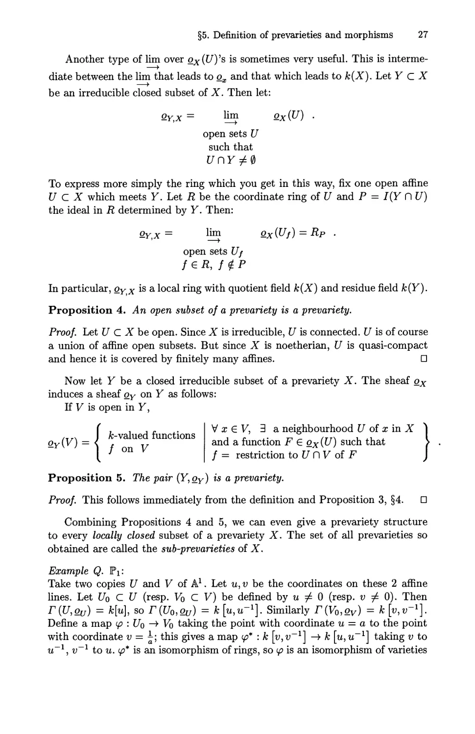
Example Q. Pi:
Take two copies U and V of A1. Let u, v be the coordinates on these 2 affine
lines. Let Uq С U (resp. Vb С V) be defined by и ф 0 (resp. и ^ 0). Then
r{U,ov) = k[u], so r(E/b,Otf) = к [щи-1]. Similarly r(V0,ov) = к [и,и].
Define a map ip : [To —> Vo taking the point with coordinate и = a to the point
with coordinate v = ^; this gives a map ip* : к [v,v~*] —> к [и,и~г] taking v to
u, v to u. ip* is an isomorphism of rings, so ip is an isomorphism of varieties
28 I. Varieties
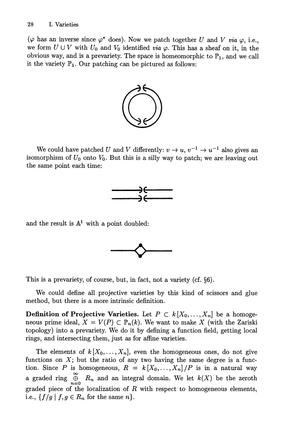
{if has an inverse since if* does). Now we patch together U and V via if, i.e.,
we form U U V with Uq and Vq identified via if. This has a sheaf on it, in the
obvious way, and is a prevariety. The space is homeomorphic to Y\, and we call
it the variety Pb Our patching can be pictured as follows:
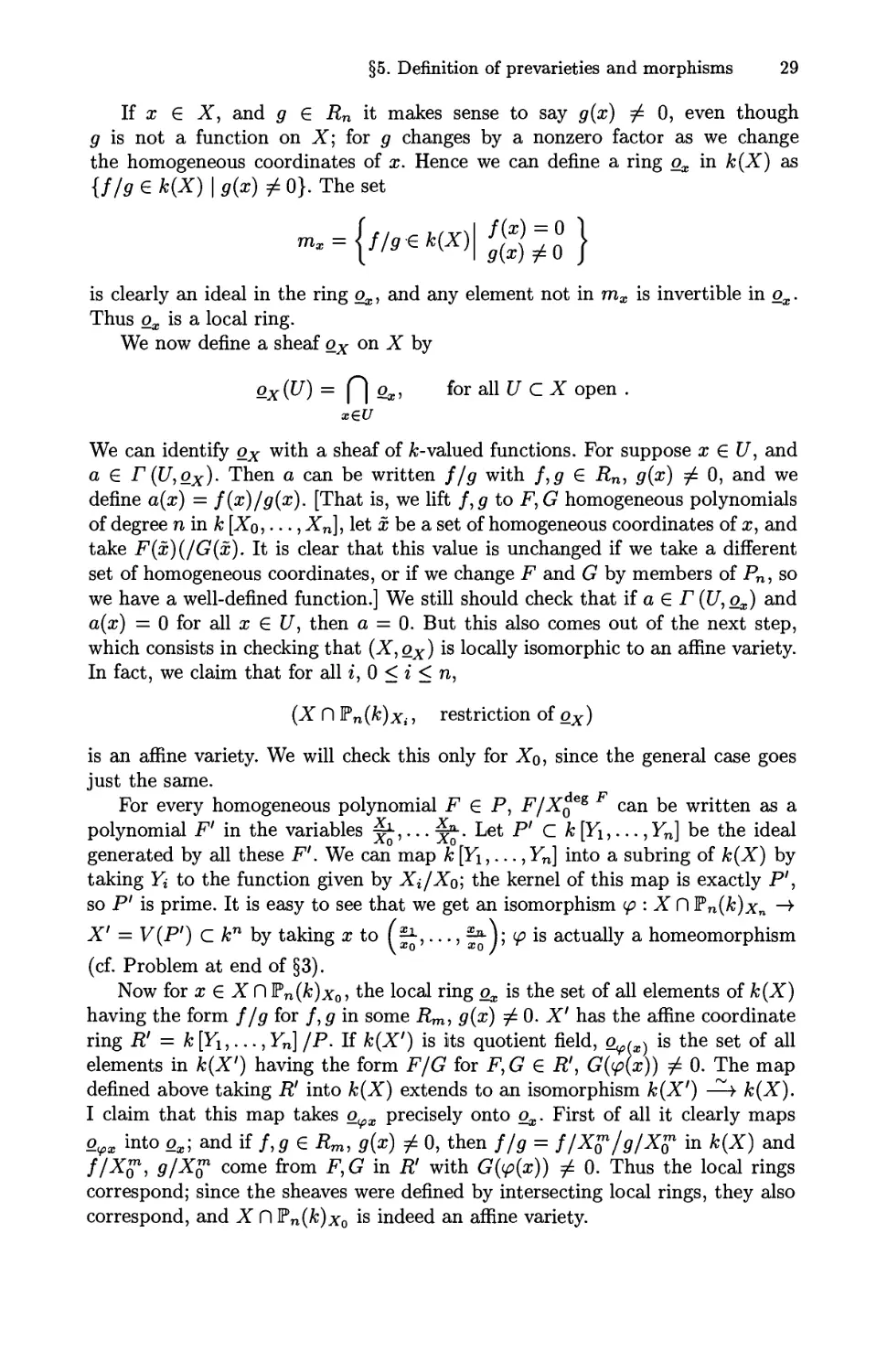
We could have patched U and V differently: v —> u, v * —> и 1 also gives an
isomorphism of Uq onto Vq. But this is a silly way to patch; we are leaving out
the same point each time:
and the result is A1 with a point doubled:
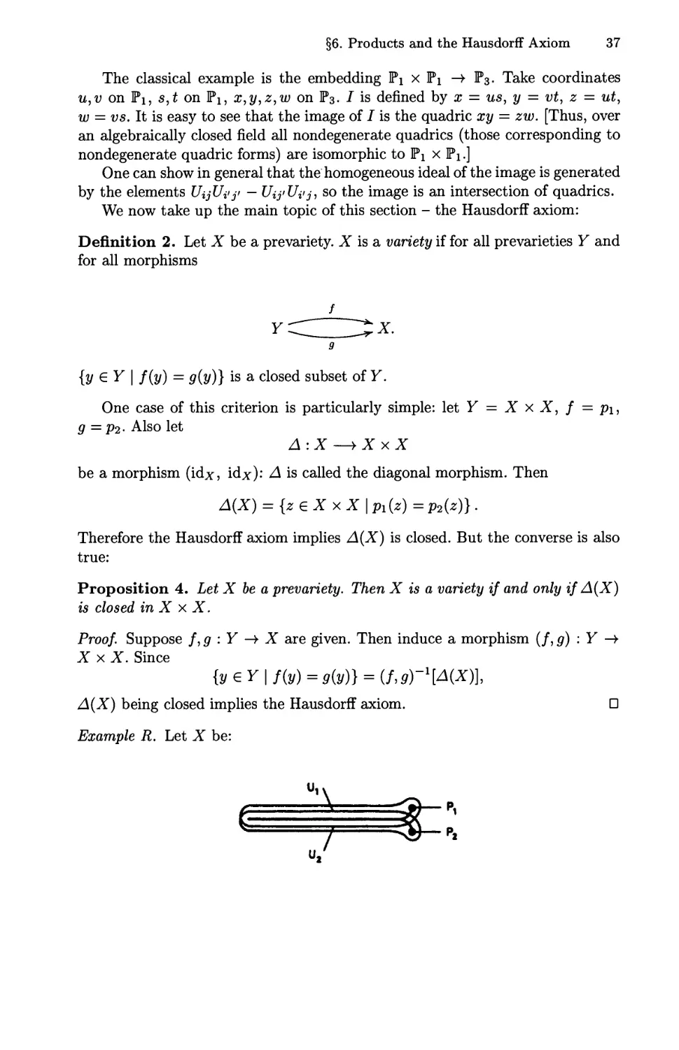
This is a prevariety, of course, but, in fact, not a variety (cf. §6).
We could define all projective varieties by this kind of scissors and glue
method, but there is a more intrinsic definition.
Definition of Projective Varieties. Let P С к [Хо,... ,Xn] be a homoge-
homogeneous prime ideal, X = V{P) С Yn{k). We want to make X (with the Zariski
topology) into a prevariety. We do it by defining a function field, getting local
rings, and intersecting them, just as for affine varieties.
The elements of k[Xo,... ,Xn], even the homogeneous ones, do not give
functions on X; but the ratio of any two having the same degree is a func-
function. Since P is homogeneous, R = k[X0,.. .,Xn] /P is in a natural way
oo
a graded ring 0 Rn and an integral domain. We let k{X) be the zeroth
n=0
graded piece of the localization of R with respect to homogeneous elements,
i-e-, {f/g | f,g £ Rn for the same n).
§5. Definition of prevarieties and morphisms 29
If x € X, and g £ Rn it makes sense to say g{x) ф 0, even though
g is not a function on X; for g changes by a nonzero factor as we change
the homogeneous coordinates of x. Hence we can define a ring ox in k{X) as
{f/g e k(X) | g(x) ф 0}. The set
is clearly an ideal in the ring o^, and any element not in mx is invertible in ox.
Thus ox is a local ring.
We now define a sheaf ox on X by
ox (U) = Pi Од., for all U С X open .
x€U
We can identify ox with a sheaf of A;-valued functions. For suppose x e U, and
a e r(U,ox). Then a can be written f/g with /, g £ Rn, g(x) ф 0, and we
define a(x) = f(x)/g(x). [That is, we lift /, g to F, G homogeneous polynomials
of degree n in к [Хо,..., Xn], let ж be a set of homogeneous coordinates of x, and
take F(x)(/G(x). It is clear that this value is unchanged if we take a different
set of homogeneous coordinates, or if we change F and G by members of Pn, so
we have a well-defined function.] We still should check that if a € Г A7,0,.) and
a(x) = 0 for all x € U, then a = 0. But this also comes out of the next step,
which consists in checking that (X,ox) is locally isomorphic to an affine variety.
In fact, we claim that for all г, 0 < г < n,
(X D fn(k)xi, restriction of ox)
is an affine variety. We will check this only for Xo, since the general case goes
just the same.
For every homogeneous polynomial FgP, F/Xq^ can be written as a
polynomial F' in the variables ^,... ^. Let P' С к [Y\,..., Yn] be the ideal
generated by all these F'. We can map k[Y\,...,Yn] into a subring of k(X) by
taking Yi to the function given by Xi/Xo; the kernel of this map is exactly P',
so P' is prime. It is easy to see that we get an isomorphism <p : X П fn(k)xn —>
X' = V(P') С kn by taking x to (I1,..., ^ J; if is actually a homeomorphism
(cf. Problem at end of §3).
Now for x e X D fn(k)x0, the local ring a,, is the set of all elements of k(X)
having the form f/g for /, g in some Rm, g(x) ф 0. X' has the affine coordinate
ring R' = к [Yi,..., Yn] /P. If k(X') is its quotient field, 2^(ж) is the set of all
elements in k(X') having the form F/G for F,G e R', G(ip(x)) Ф 0. The map
defined above taking R' into k(X) extends to an isomorphism k(X') —> k(X).
I claim that this map takes o(fiX precisely onto o^.. First of all it clearly maps
ovx into ox; and if f,g e Rm, g{x) ф 0, then f/g = f/X^jg/X^ in k{X) and
f/Xfi1, g/X^ come from F,G in R' with G(<p(x)) ф 0. Thus the local rings
correspond; since the sheaves were defined by intersecting local rings, they also
correspond, and X D fn(k)x0 is indeed an affine variety.
30 I. Varieties
Definition 5. Let X and Y be prevarieties. A map / : X —> Y is a morphism
if / is continuous and, for all open sets V in Y,
Proposition 6. Let f : X -> Y be any map. Let (Vi) be a collection of open
affine subsets covering Y. Suppose that {Ui} is an open covering of X such that
1) f(Ui) С Vi and 2) f* maps Г (Vi,oY) into Г (Ui,ox). Then f is a morphism.
Proof. We may assume the Ui are affine; for if U С Ui is affine, /* certainly
maps r(Vi,oY) into Г (U,ox), and we can replace Ui by a set of affines that
cover Ui. First of all, the restriction fi of / to a map from Ui to Ц, is a morphism.
In fact, the homomorphism
is also induced by some morphism gi : Ui —>• Vi (Proposition 1, §3). And since
the functions in r(Vi,oY) separate points, a map from Ui to Vi is determined
by the contravariant map from F(Ui,ox) to r(Vi,oY). Therefore fi = gi and
fi is a morphism. In particular, fi is continuous and this implies immediately
that / itself is continuous. It remains to check that /* always takes sections oY
to sections ox. But if У С У is open, and g € Г (V,oY), then g • / is at least a
section of ox on the sets f~l (V П Vi), hence on the sets f-1(V) П Ui. Since ox
is a sheaf, g • f is actually a section of ox in f~l (V). D
To illustrate the meaning of our definitions, it seems worthwhile to work out
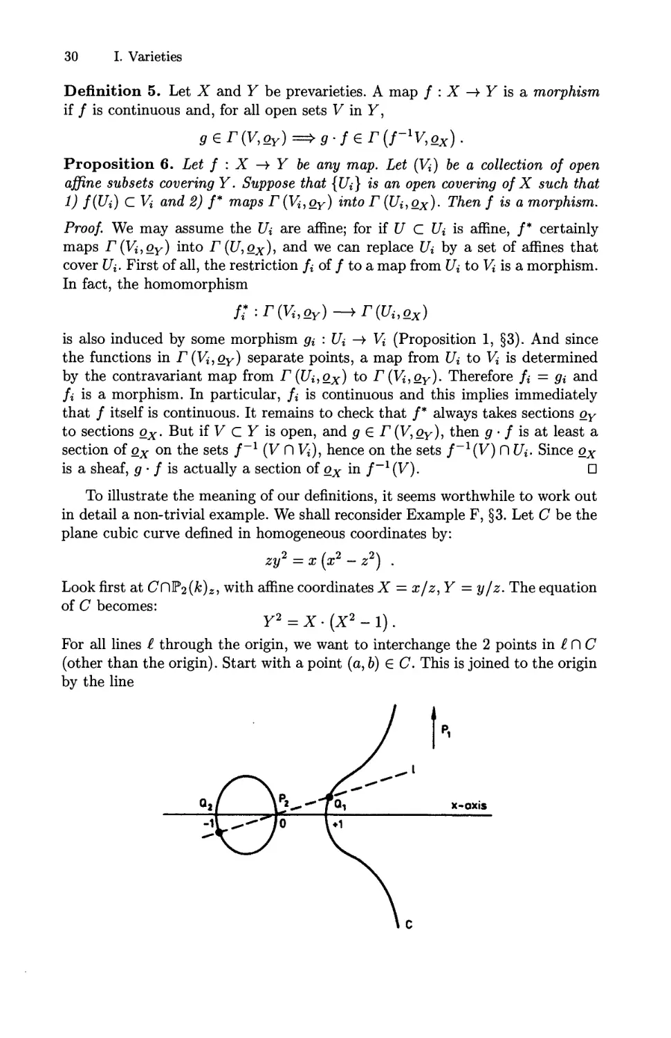
in detail a non-trivial example. We shall reconsider Example F, §3. Let С be the
plane cubic curve defined in homogeneous coordinates by:
zy2 = x (x2 - z2) .
Look first at СПР2(А;J, with affine coordinates X = x/z, Y = y/z. The equation
of С becomes:
Y2 = X ■ (X2 - 1).
For all lines I through the origin, we want to interchange the 2 points in l П С
(other than the origin). Start with a point (a, b) £ C. This is joined to the origin
by the line
§5. Definition of prevaxieties and morphisms 31
X = at
Y = Ы.
Intersecting this with the cubic, we get the equation
bH2 = at(a2t2-l)
or
0 = at(t - 1) (a2t + 1) .
Thus the 2nd point of intersection is given by t = —I/a2. In other words, the
morphism on С is to be given by:
These are not polynomials, so at any rate they do not define a map from this
affine piece of С into itself; this is as it should be, since as we can see from the
drawing, we want the origin itself to go to the one point at infinity on the cubic.
To describe the subsets on which we will get a morphism, we must throw out
the various "bad" points one at a time. We need names for them:
Pi = @,1,0) (the only point at oo with respect to the
affine piece X, Y)
P2 = @,0,1) (the origin)
/V ~ / \ 'n -i\ \ other points on the X-axis .
ЧГ2 = (-1>U, 1) J
The morphism - call it / - should interchange Pi and P2, Q\ and Q2. Define
V\ = C-{PUP2)
U2 = C-iP^QuQ^
U3 = C-{P2,QUQ2}
V2 = С-{P2,Q1,Q2} = С nf2(k)y.
Then 1) Ui,U2, Щ is an open covering of C, 2) V\, V2 is an affine open covering of
C, and 3) if / is defined set-theoretically as above, then f(Ui) С Vi, f{U2) С V2
and /A1з) С V\. Therefore, by Proposition 6, it suffices to check that
and
Г[Г(У210с)] С
and then it follows that / is a morphism. In more down to earth terms: note
that X, Y are affine coordinates in Vi and
32 I. Varieties
S = x/y
T = z/y
are affine coordinates in V2. Then what we have to check is that /, described via
one of these 2 sets of coordinates, is given by polynomials in U\, U2, and U3.
In U\\ X,Y and 1/X are functions in r(Ui,oc). Thus describing the image
point also by coordinates X, Y, f is given by:
and these are polynomials in a, 6, I/a.
In JJi'- X, Y and ^ty are functions in Г A/2,0^1). Describe the image of the
point (a, 6) by coordinates S, T now:
S[f(a,b)] = a/b
T[f(a,b)} = -a2/b.
This does not look very promising until we use the relation b2 = a- (a2 — 1)
to rewrite these as:
S = b/a?-l
T = -ab/a2 - 1
which are polynomials in a, 6, I/a2 — 1.
In £/3: S and T are functions in Г^Цз,^). Describe the image of the point
S = с, Т = d by coordinates X, Y:
X[f(c,d)] = -d/c
Y[f(c,d)} = -d/c2.
However с and d are related by d = с • (с2 — d2), so we get:
X = d2-c2
Y = d(c2-d?)-c.
D
Problem. Generalize the result by which we covered Pn by open affine sets as
follows: for all homogeneous polynomials H G к [Xo,... ,Xn] of positive degree,
show that Рп(&)я 1S an an<me variety.
§6. Products and the Hausdorff Axiom 33
§6. Products and the Hausdorff Axiom
We want to define the product X x Y of any two prevarieties X, Y. Now we
will certainly want to have An x Am = An+m. But the product of the Zariski
topologies in An and Am does not give the Zariski topology in An+m; in A1 x A1,
for instance, the only closed sets in the product topology are finite unions of
horizontal and vertical lines. The only reliable way to find the correct definition
is to use the general category-theoretic definition of product.
Definition 1. Let С be a category, X, Y objects in C. An object Z plus two
morphisms
X
Z
\
Y
is a product if it has the following universal mapping property: for all objects W
and morphisms
W
X
Y
there is a unique morphism t : W -> Z such that r = p-t, s = q-1, i.e., such
that
commutes. The induced morphism t in this situation will always be denoted
(r, s). We call p and q the projections of the product onto its factors. Clearly a
product, if it exists, is unique up to a unique isomorphism commuting with the
projections.
34 I. Varieties
The requirement of the definition can be rephrased to say hom(W, Z) -^>
Ьот(И^, X) x Ьот(И^, Y) (under the obvious map induced by p and q).
We shall prove that products exist in the category of prevarieties over k. Note
that we have no choice for the underlying set; for if X x Y is a product of the
prevarieties X and Y, X x Y as a point set must be the usual product of the
point sets X and Y. To see this, let W be a simple point; this is a prevariety (A0,
in fact). The maps of W to any prevariety S clearly correspond to the points of
S, and by definition hom(W,X x Y) ~ hom(W,X) x hom(W,Y).
Proposition 1. Let X and Y be affine varieties, with coordinate rings R and
S. Then
1) there is a product prevariety X x Y.
2) X xY is affine with coordinate ring R <g>j. S.
3) a basis of the topology is given by the open sets
4) 2(Ж)У) is the localization of ox ®k Qy at the maximal ideal mx • oy + ox • my.
Proof. We recall the following result from commutative algebra: let R and S be
integral domains over the algebraically closed field k. Then R <g>j. S is an integral
domain. [Cf. Zariski-Samuel, vol. 1, Ch. 3, §15.]
Represent
ХСГ as V(/i,...,/mi) .
FCP as V(gi,...,gm2) .
Then the set X x Y с кП1+П2 is the locus of zeroes of fj(Xi),gj(Yi) in
к [Xi,..., Xni, Yi,..., Yn2\. Moreover
But R <8>k S is an integral domain; hence (fj,gj) is prime, X x Y is irreducible,
and R <g>j. 5 is its coordinate ring.
This gives us an affine variety X xY. The next step is to prove that it is a
categorical product. We have natural projections
p,q:XxY —> X,Y [e.g., p(xu ... ,yn2) = (xu ... ,sni)]
which are clearly morphisms. Suppose we are given morphisms f : Z -> X,
s : Z -> Y. There is just one map of point sets t: Z ->• X xY such that r = p-t,
s = g • t (since X x Y as a point set is the product of -X" and Y), and to verify
the universal mapping property we need only check that t is always a morphism.
But this is simple. Since X x Y is affine, it suffices to check that g G
Г (X x Y,oXxY) =>■ p-t G T(Z,oz). NowT(X x У,оХхУ) is generated by the
images of Г (X, ox) = R and Г (У, oY) = S. Both of these by composition with t
§6. Products and the Hausdorff Axiom 35
go into Г (Z,o%) since r and s are morphisms; therefore all of Г (X x Y,QXxY)
goes into Г (Z,oz).
We have proved 1) and 2), and 3) follows from 2). Now 0(Ж)У) is the localization
of R <S>k S at the ideal of all functions vanishing at (x,y). Clearly R <S>k S С
0.x ®k Qy С О(ж у), and therefore we can get 0(Ж)У) by localizing ox <g>k oy at the
ideal of all functions in it vanishing at (x,y). We claim that ideal is precisely
mx -Qy + ox -niy. Evidently all these functions do vanish there. Conversely, if we
take any h = £ /i ® 9% € ox®koy, with, say, /,-(ж) = a<, gi(y) = A, then we
claim /i — X) aiA £ "Ъ • 2y + Qx • my. Indeed it equals
D
We can now "glue together" these affine products to obtain:
Theorem 2. Let X and Y be prevarieties over k. Then they have a product.
Proof. We start, of course, with the product set. For all open affine U С X,
V С Y and all finite sets of elements fa G Г(и,ох), gi G r(V,oY) we form
(U x V)sfi9i; these we take as a basis of the open sets. (They do form a basis,
since (U x V)sfigi П (?/' x V')r/(e;. contains (U" x V")^/^..^/^»., where ?7"
[resp. V"] is an affine contained in U П C/"' [resp. У П V'].) Note that ont/хУ
this induces the topology of their true product.
Let К be the quotient field of k(X) <8>д. fc(F) [which, as before, is an integral
domain]. For x G X, у G Y we let О(Х)У) С iiT be the localization of ox ®k Qy at
the ideal mx • oy + ox • my, and we set
= П 2(»,y)'
This gives us a sheaf of functions. Furthermore, it coincides on each U xV (U,V
affine) with the product of the affine varieties. Clearly X x Y is connected and
covered by finitely many affines, so it is a prevariety.
Now suppose Z -^> X, Z -^> У are morphisms. Set-theoretically there is
a unique map (r, s) : Z -> X x Y composing properly with the projections; we
want to check that it is a morphism. For each U in X, V in Y affine, look at
Zu,v = r~1(U) П s~1(V). These are open sets covering Z, and since being a
morphism is a local property it is enough to prove (r, s) \ Zu.v is a morphism.
That is, we may assume r{Z) С U, s(Z) С V. But in the last proposition we
saw that then the product map Z ->• U x V is a morphism; and G x У is an
open subprevariety of X x Y, so the composite map Z-^UxV^XxY is а
morphism.
Remarks. I. If U is any open subprevariety of X, then t/ x Y is an open subpre-
subprevariety of X x Y.
II. If Z is a closed subprevariety of X, then Z x Y is a closed subprevariety
of X x У. [It is enough to prove (Z C\U) xV & closed subprevariety of U x V
for U, V affine, and this is easily checked.]
36 I. Varieties
Theorem 3. The product of two projective varieties is a projective variety.
Proof. Since a closed subvariety of a projective variety is a projective variety, it
is enough to show Pn x Pm is a projective variety. In fact, we can embed it as a
closed subvariety of Pnm+n+m.
Take homogeneous coordinates Xo,.. ■, Xn in Pn, Yo,..., Ym in Pm, and Uij
(i = 0,..., n, j = 0,..., m) in P(n+1)(m+1)_1. Define a map:
/.ГО» \у Ш> i Ш)
. Jrn X Jrm У Jrnm+n+m
by
, ч / ч a point with homogeneous coordinates
(xo,...,xn)x(yo,...,ym)—> TT._rqi
[This makes sense; multiplying all X{ for all yj by A multiplies all Uij by A; and
some Uij is nonzero.] Clearly
We claim that first / is injective. Assume that for some А ф 0, Xiyj = Xx^y'j for
all г and j; then we want to prove that for some fi, v ф 0, Xi = fj,x't, yj = vy'y
We may by symmetry assume x0 ф 0, y0 ф 0. Then we have 0 Ф xoyo = x'oy'o, so
x'o Ф^чУоФ 0- We have Xi/x0 = Xiyo/xoyo = х[уЬ/х'оу'о = х[/х'о and similarly
for yj/yo- This proves what we want.
Now we claim / is an isomorphism of (Pn)x; x (^m)y. onto a closed subva-
subvariety of (Рп+т+пт)с/;.- We may assume i = 0,j = 0 for simplicity. On (Pn)x0
we take affine coordinates Si = Xi/Xo, i = 1,... ,n. On (Pm)y0 we take affine
coordinates Tj = Yj/Y0, j = 1,... ,m. On (Pn+m+nm)[/oo we take affine coordi-
coordinates Rij = Uij/Uoo, i > 1 or j > 1. In these coordinates, / takes (s,t) to the
point
Rij = Sitj if i, j > 1
^iO — Si, Roj = tj .
Hence the image is the locus of points satisfying Rij = RioRoj for all i,j > 1.
This is certainly closed. Its affine coordinate ring is k[Rij] / (Rij — R^Roj),
which is clearly isomorphic to the polynomial ring к [Rio, Roj]. Under /*, this is
mapped isomorphically to к [Si,Tj] which is the affine coordinate ring of (Pn)x0 x
(Pm)Fo. Hence we do have an isomorphism.
Let Z = J(Pn x Pm). Since Z П (Pn+m+nm)v.. is closed for all i,j, Z is
closed. / is a homeomorphism on each of these affines, so it is a homeomorphism
globally, and in particular Z is irreducible. Thus Z is a projective variety. Since
/ is an isomorphism on each affine piece, it is an isomorphism globally and hence
Z is isomorphic to Pn x Pm. D
§6. Products and the Hausdorff Axiom 37
The classical example is the embedding Pi x Pi -»• P3. Take coordinates
u,v on Pi, s,t on Pi, x,y,z,w on P3. / is defined by x = us, у = vt, z = ut,
w = vs. It is easy to see that the image of / is the quadric xy = zw. [Thus, over
an algebraically closed field all nondegenerate quadrics (those corresponding to
nondegenerate quadric forms) are isomorphic to Pi x Pi.]
One can show in general that the homogeneous ideal of the image is generated
by the elements UijUi'j' — Uij'Ui'j, so the image is an intersection of quadrics.
We now take up the main topic of this section - the Hausdorff axiom:
Definition 2. Let X be a prevariety. X is a variety if for all prevarieties Y and
for all morphisms
9
{y e Y I f(y) = g(y)} is a closed subset of Y.
One case of this criterion is particularly simple: let Y = X x X, f =
g = p2. Also let
A:X -^X xX
be a morphism (idx, idx)- ^ is called the diagonal morphism. Then
= {zeXxX\Pl(z)=p2(z)}.
Therefore the Hausdorff axiom implies A{X) is closed. But the converse is also
true:
Proposition 4. Let X be a prevariety. Then X is a variety if and only if A(X)
is closed in X x X.
Proof. Suppose f,g : Y ->• X are given. Then induce a morphism (/, g) : Y ->•
X x X. Since
A{X) being closed implies the Hausdorff axiom. D
Example R. Let X be:
7
38
I. Varieties
i.e., 2 copies U\,U2 of A1, say with coordinates X\ and ж2, patched by the map
Xi = X2 on the open sets x\ Ф 0 and x-i ф 0. Consider the isomorphisms of A1
with each of the 2 copies:
О
X
с
Call these гьг2 : A1 -)• X. Then
{у G A1 | ii(y) = «2B/)} = A1 — {0}
is not closed in A1, hence X is not a variety.
Remarks. I. A subprevariety of a variety is a variety. A product of 2 varieties is
a variety.
II. An affine variety is a variety: in fact, if X is affine, Y is an arbitrary
prevariety, and f,g :Y ->• X are 2 morphisms, then
locus of zeroes of the functions
s.f.-s.g., a\\ser(X,ox)
and this set is closed.
III. From II., we can check that if f,g : Y -> X are any morphisms of any
prevarieties, then {y G Y \ f(y) = g(y)} is always locally closed. In fact, call this
set Z. If z G Z, let У be an affine open neighbourhood of f{z) (= р(г)). Then
in the affine
variety
and this set is closed since У is a true variety.
IV. Another useful way to use the Hausdorff property is this: if / : X ->• Y is
a morphism of prevarieties and Y is a variety, then the image of the morphism
which is the ргарЛ of /, is closed. Moreover, if we let Гд be this image, then Г/
is even a closed subprevariety of X x Y isomorphic to X under the mutually
inverse morphisms:
(id,/)
X
§6. Products and the Hausdorff Axiom 39
(here pi : X x Y -> X is the projection).
Proposition 5. Let X be a prevariety. Assume that for all x,y G X there is an
open affine U containing both x and y. Then X is a variety.
Proof. Suppose f,g :Y -> X are 2 morphisms such that Z = {y G Y \ f(y) = g(y)}
is not closed. Let z G Z, x = f(z), у = g(z). By assumption, there is an open
affine V containing x and y. Let U = f~1(V) П g~1(V): U is an open neigh-
neighbourhood of Z. If f',g' are the restrictions of f,g to morphisms from U to V,
then
ZnU = {yeU\f'(y) =
is closed in U, since V, being affine, is a variety. Therefore z G Z C\U, and Z is
closed. D
Corollary. Every protective variety X is a variety.
Proof. For all x,y e №n(k), there is a hyperplane not containing x or y, i.e., an
element H = ЕоцХг G k[X0,...,Xn] such that x,y G Рп(&)я- But Рп(&)я is
affine, hence X П Рп(&)я is open and affine in X. D
Proposition 6. Let X be a variety, and let U, V be affine open subsets with
coordinate rings R, S. Then U C\V is an affine open subset with coordinate ring
R • S (the compositum being formed in k(X)).
Proof. U x V is an affine open subset of X x X with coordinate ring R®k S. Let
Z = A(X). Then Z П (U x V) is a closed subset of U x V isomorphic via A to
UC\ V. Since A is an isomorphism, Zn(U xV) is irreducible, hence it is a closed
subvariety of U x V. Therefore it is affine, and its coordinate ring T is a quotient
of the coordinate ring of U x V. But it is also open in Z, hence Z С k(Z), i.e.,
T is the image of R <8>k S in k(Z). Again since Л is an isomorphism, this proves
that
UnV = A~1{Zn(UxV)}
is an open affine subvariety of X, and that its coordinate ring is A*(R (8) S) in
k(X). But A*(f®g) = f-g, hence A*(R<g>S) = R■ S. D
Problem. Prove the following converse: let X be a prevariety, {Ui} an affine
open covering of X. Let Ri be the coordinate ring of Ui. Then if Ui П Uj is an
affine subset of X with coordinate ring Ri • Rj, X is a variety.
Zariski and Chevalley have used a quite different definition of a variety which
is useful for many questions, especially "birational" ones, i.e., questions dealing
with various different prevarieties with a common function field.
Definition 3. Let О С О' be local rings. We say O' dominates О or O' > O,
if m' D m (equivalently m' ПО = m) where m, m' are the maximal ideals of O,
O' respectively.
40 I. Varieties
Local Criterion: Let X be a prevariety. Then X is a variety if and only if for
all x, у G X such that x ф у, there is no local ring О С k{X) such that О > q_x
and (9 > oy.
The fact that this holds for varieties will be proven in Ch. II, §6. We omit the
converse which we will not use. If one starts with this criterion, however, one can
take the elegant Chevalley-Nagata definition of a variety: we identify a variety X
with the set of local rings ox. For this definition, a variety is a finitely generated
field extension К oik plus a collection of local subrings of К satisfying various
conditions. [Notice: the topology can be recovered as follows - for each / G K,
let Uf be the set of those local rings in X containing /.]
Problem. Let X С Pn be defined by a homogeneous ideal P С к [Хо,..., Xn].
Let P define the affine variety X* С An+1. Show that for all г,
f Subset of X* 1 ^ Ai / Subset of X 1
\ where 1^0 J" X \ where X{ ф 0 j "
§7. Dimension
Definition 1. Let X be a variety. dimX = tr.d.kk(X).
If U is an open and nonempty set in X, dimU = dimX, since k{U) = k(X).
Since к is algebraically closed, the following are equivalent:
)
ii) k(X) = к
iii) X is a point.
Proposition 1. LetY be a proper closed subvariety ofX. ThendimY < dimX.
Proof .
Lemma. Let R be an integral domain over к, Р С R a prime. Then
tr.d.kR > tr.d.kR/P, with equality only if P = {0} or both sides are oo. [By
convention, tr.d.R is the tr.d. of the quotient field of R.J
Proof. Say P ф 0, tr.d.kR = n < oo. If the statement is false, there are n
elements X\,..., xn in R such that their images xi in R/P are algebraically
independent. Let 0 ф p G P. Then p,Xi,...,xn cannot be algebraically inde-
independent over к, so there is a polynomial P(Y,Xi,...,Xn) over к such that
P (p, x\,..., xn) = 0. Since R is an integral domain, we may assume P is irre-
irreducible. The polynomial P cannot equal aY, a G /г, since p ф 0. Therefore P is
not even a multiple of Y. But then P @,xi,...,xn) = 0 in Л/Р is a nontrivial
relation on the X\,...,xn-
Now choose [/Clan open affine set with UOY ф 0. Let R be the coordinate
ring of U, P the prime ideal corresponding to the closed set UdY. Then P ф 0,
since U C\Y фи. к(Х) is the quotient field of Л, and /г(У) is the quotient field
of R/P. Therefore the Proposition follows immediately from the lemma. D
§7. Dimension 41
In the situation of this Proposition, dimX - dim У will be called the codi-
mension of X in Y. This is half of what we want so that our definition gives a
good dimension function. The other half is that it does not go down too much.
Theorem 2. Let X be a variety, U С X open, g G r(U,ox), Z an irreducible
component of {x G U \ g{x) = 0}. Then if g фО, dim Z = dimX — 1.
Proof. Take Uo С U an open affine set with Uo П Z ф 0. Let R = r(U0,ox),
f = resu,uo9 £ R- Then Z П Uo corresponds to a prime P С R. Z is by hypo-
hypothesis a maximal irreducible subset of the locus g = 0, so Z П t/o is a maximal
irreducible subset of the locus / = 0, i.e., P is a maximal prime containing /.
Thus we have translated Theorem 2 into:
Algebraic Version (Krull's Principal Ideal Theorem). Let R be a finitely
generated integral domain over k, f G R, P an isolated prime ideal of (/) (i.e.,
minimal among the prime ideals containing it). Then if f ф 0, tr.d.kR/P =
tv.d.kR- 1.
This is a standard result in commutative algebra (cf. for example, Zariski-
Samuel, vol. 2, Ch. 7, §7). However there is a fairly straightforward and geometric
proof, using only the Noether normalization lemma and based on the Norm, so
I think it is worthwhile proving the algebraic version too. This proof is due to
J. Tate.
At this point, it is convenient to translate the results of §1 into the geometric
framework that we have built up:
Definition 2. Let / : X ->• Y be a morphism of affine varieties. Let R and
S be the coordinate rings of X and Y, and let /* : S ->• R be the induced
homeomorphism. Then / is finite if R is integrally dependent on the subring
f*(S).
Note that the restriction of a finite morphism from X to Y to a closed
subvariety Z of X is also finite. Examples N and О in §3 are finite morphisms,
but example P is not. The main properties of finite morphisms are the following:
Proposition 2. Let f : X ->• Z be a finite morphism of affine varieties.
A.) Then f is a closed map, i.e., maps closed sets onto closed sets.
B.) For all у eY, f~l(y) is a finite set.
C.) f is surjective if and only if the corresponding map f* of coordinate rings
is injective.
Proof. Let / be dual to the map f*:S->Rof coordinate rings. As usual, the
maps V, / set up bijections between the points of X (resp. Y) and the maximal
ideals m of R (resp. S). If V(A) is a closed set in X, then f(V(A)) corresponds
to the set of maximal ideals /* (m), m с R a maximal ideal containing A.
But by the going-up theorem, whenever R D S and R is integral over S every
prime ideal P С S is of the form P' П S for some prime ideal P' С R (cf. §1).
If В = f*~\A), apply the going-up theorem to S/B С R/A; therefore f(V(A))
42 I. Varieties
corresponds to the set of maximal ideals m such that m D B, i.e., to V(B).
Therefore, / is closed. Moreover, f(X) = Y if and only if Ker(/*) = @). B.) is
equivalent to saying that for all maximal ideals m С S, there are only a finite
number of maximal ideals ml С R such that m = f* {ml). Since such ml all
contain f*(m) • R, it is enough to check that R/f*(m) • R contains only a finite
number of maximal ideals. But R/f*(m) • R is integral over S/m, i.e., it is a
finite-dimensional algebra over k, so this is clear. D
Via this concept, we can state:
Geometric form of Noether's normalization lemma. Let X be an affine
variety of dimension n. Then there exists a finite surjective morphism ж:
Proof of Theorem 2. We first reduce the proof to the case P = \/(/), i.e.,
geometrically, to the case Z = V((f)). To do this, look back at the way in which
we related the geometric and algebraic versions of the Theorem. Note that the
algebraic version is essentially identical to Theorem 2 in the case X = U is affine
with coordinate ring R. Suppose we have the decomposition
(/) = P П P[ П ... П Pi
in R. Geometrically, if Z[ = V (P/), this means that Z, Z{,..., Z[ are the com-
components of V((f)). Now we pick an affine open Uq С X such that:
Uo П Z ф 0
Uo П Z[ = 0, i = l,...,t.
For example, let Uo = Xg, where:
деР{П...ПР1, д^Р.
Then replace X by Uo, R by R(g), and in the new set-up,
Vuo((f)) = Vx((f))nU0
= ZHUo
is irreducible; hence in R^, y/{f) = P • R(g) is prime.
Now use the normalization lemma to find a morphism as follows:
X R
k[Xu...,Xn] = S.
Let К (resp. L) be the quotient field of R (resp. S). Then K/L is a finite algebraic
extension. Let
§7. Dimension 43
/o =
Then I claim /o G 5 and
If we prove (*), the theorem follows. For R/P is an integral extension of S/SDP,
so
tr.d.kR/P = tr.d.fcS/S П P .
But 5 is a UFD, so the primary decomposition of a principal ideal in S is just the
product of decomposition of the generator into irreducible elements. Therefore
(*) implies that /o is a unit times /q0 for some integer £ and some irreducible
/oo, and that P П S = (/oo)- Hence
tr.d.fcS/S П P = tv.d.kk [Xu... ,Xn] /(/oo) = n.
We check first that /0 G P П S. Let
be the irreducible equation satisfied by / over the field L. Then /o is a power
(an)m of an. Moreover, all the a^s are symmetric functions in the conjugates of
/ (in some normal extension of L): therefore the сц are elements of L integrally
dependent on S. Therefore ai G S. In particular, /o = a™ G S, and since
— an ' \J +aiJ +... + an)
- J • \an J +an alt +--- + an <hi-l) + JO ,
/o G P too.
Finally suppose g G P П 5. Then g e P = y/(fj, hence
n _ f h some integer n ,
5 ~ ; " ' some Л G Л .
Taking norms, we find that
9n[K:L] = NK/L(gn)
= NK/L(f)-NK/L(h)e(f0)
since NK/ih is an element of S, by the reasoning used before. Therefore g G
a/(/o), and (*) is proven. D
Definition 3. Let X be a variety, and let Z С X be a closed subset. Then Z
has риге dimension r if each of its components has dimension r (similarly for
pure codimension r).
44 I. Varieties
The conclusion of Theorem 2 may be stated as: V((g)) has pure codimen-
sion 1, for any non-zero g G Г(Х,ох). The Theorem has an obvious converse:
Suppose Z is an irreducible closed subset of a variety X of codimension 1. Then
for all open sets U such that Z C\U Ф 0 and for all non-zero functions f on U
vanishing on Z, Z П U is a component of / = 0. In fact, if W were a component
of / = 0 containing Z C\U, then we have
dimX > dimW > dim ZnU = dimX - 1
hence W = Z C\U by Proposition 1.
Corollary 1. Let X be a variety and Z a maximal closed irreducible subset,
smaller than X itself. Then dim Z = dimX — 1.
Corollary 2 (Topological characterization of dimension). Suppose
is any maximal chain of closed irreducible subsets of X. Then dimX = r.
Proof. Induction on dimX.
Corollary 3. Let X be a variety and let Z be a component of V ((/i, •. •, fr)),
where /i,..., fT G Г (X,ox). Then codim Z <r.
Proof. Induction on r. Z is an irreducible subset of V ((/i,..., Л—1)M so it is
contained in some component Z' of V ((/i,..., Л—i)). Then Z is a component of
Z'nV((fr)), since Z'r\V((fr)) СУ((/Ь..., fr)). By induction codim Z' < r-1.
If fr e 0 on Z', Z — Z'. If /r does not vanish identically on Z', then by the
theorem, dim Z = dim Z' — 1, so codim Z <r. D
Of course, equality need not hold in the above result: e.g., take fi = .. • = fi,
r> 1.
Corollary 4. Let U be an affine variety, Z a closed irreducible subset. Let r =
codim Z. Then there exist f\,..., fr inR = Г(U,Оц) such that Z is a component
ofV((fu...,fr)).
Proof. In fact, we prove the following. Let Z\ D Z2 D ... D ZT = Z be a chain of
irreducibles with codim Zi = i (by Cor. 2). Then there are f\,..., fr in R such
that Zs is a component of V ((/i,..., fs)) and all components of V ((/i,...,/«))
have codim s.
We prove this by induction on s. For s = 1, take f\ G I(Zi), f\ ф 0,
and we have just the converse of the theorem. Now say /i,..., /s-i have been
chosen. Let Zs-\ = Yi,...,Yt be the components of V ((/i,..., Л-i))- For all
г, Zs 75 Yi (because of their dimensions), so I(Yi) ~fi I(ZS). Since the I(Yi) are
prime, ULi ОД) 2 Hzs) [Zariski-Samuel, vol. 1, p. 215; Bourbaki, Ch. 2, p.
70]. Hence we can choose an element fs G I(ZS), 's ^ Ui=i
§7. Dimension 45
If Y is any component of V ((/i,..., fs)), then (as in the proof of Cor. 3) Y
is a component of Yi П V ((/s)) for some г. Since fs is not identically zero on Y{,
dim У = dimYi — 1, so codim Y = s.
By the choice of fs, Zs С V ((/i,..., /s)). Being irreducible, Zs is contained
in some component of V ((/i,..., fs)), and it must equal this component since
it has the same dimension. . D
In the theory of local rings, it is shown that one can attach to every noetherian
local ring О an integer called its Krull dimension. This number is defined as either
a) the length r of the longest chain of prime ideals:
PogP1g...gPn = M
(M the maximal ideal of O)
or b) the least integer n such that there exist elements /i,..., fn G M for
which
(Cf. Zariski-Samuel, vol. 1, pp. 240-242; vol. 2, p. 288. Also, cf. Serre, Algebre Lo-
Locale, Ch. 3B). Recall that in §5 we attached a local ring oz x to every irreducible
closed subset Z of every variety X. We now have:
Corollary 5. The Krull dimension ozx is dimX — dimZ.
Proof. By Corollary 2, for all maximal chains of irreducible closed subvarieties:
n = dim X — dim Z. But it is not hard to check that there is an order reversing
isomorphism between the set of irreducible closed subvarieties Y and X contain-
containing Z, and the set of prime ideals P С Qz x. Or else, use the second definition
of Krull dimension: first note that if /i,..., /n G Qz x, then
Mz,x =
if and only if there is an open set U С X such that
a) UnZ^iH,
b) /ь...,/пег(г7,ох),
с) UnZ = V((fu...Jn)).
Then using Corollaries 3 and 4, it follows that the smallest n for which such /j's
exist is dim X — dim Z. D
Suppose Z С X is irreducible and of codimension 1. A natural question to
ask is whether, for all у e Z, there is some neighbourhood U of у in X and
some function / e Г (U,ox) such that Z П U is not just a component of / = 0,
but actually equal to the locus / = 0. More generally, if Z С X is a closed
subset of pure codimension r, one may ask whether, for all у G Z, there is a
neighbourhood U of у and functions /b ..., fr e Г (U, ox) such that
46 I. Varieties
znu = v«fu...,fr)) .
This is unfortunately not always true even in the special case where Z is ir-
irreducible of codimension 1. A closed set Z with this property is often referred
to as a local set-theoretic complete intersection and it has many other special
properties. There is one case where we can say something however:
Proposition 4. Let X be an affine variety with coordinate ring R. Assume R
is a UFD. Then every closed subset Z С X of pure codimension 1 equals V((f))
for some f G R.
Proof. Since R is a UFD, every minimal prime ideal of R is principal [i.e., say
P С R is minimal and prime. Let /eP. Since P is prime, P contains one of
the prime factors /' of /. By the UFD property, (/') is also a prime ideal and
since (/') С P, we must have (/') = P]. Let Z\,..., Zt be the components of Z.
Then / ((Zi),..., I(Zt)) are minimal prime ideals. If I(Zi) = (fi), then
Z = V((fu...,ft)) .
D
Proposition 5. dimX x Y = dim-X" + dimF.
The proof is easy.
The results and methods of this section all have projective formulations which
give some global as well as some local information:
Let X С Pn(fc) be a projective variety, and let I(X) С к [Xo,... ,Xn] be its
ideal.
Theorem 2*. /// G к [Xo,..., Xn] is homogeneous and not a constant and
f $ I, then X П V((/)) is non-empty and of pure codimension 1 in X, unless
Proof. All this follows from Theorem 2, except for the fact that X П V((/)) is
not empty if dimX > 1. But let X* С An+1 be the cone over X, i.e., the affine
variety defined by the ideal I(X) in k[X0,.. .,Xn]. By the problem in §6, we
know that dimX* = dimX + 1, hence dimX > 2. Let V*((/)) be the locus
/ = 0 in An+1. Since
therefore X* n V*((/)) Ф 0 and by Theorem 2, X* П V*((/)) has a compo-
component of dimension at least 1. Therefore X* П V*((/)) contains points other than
@,0,... ,0); but the affine coordinates of such points are homogeneous coordi-
coordinates of points in X П V((/)). □
Corollary 3*. If fi,. ..,fr G к [Xo,... ,Xn] are homogeneous and not con-
constants, then all components of X П V ((/i,... ,/r)) have codimension at most
r in X. And if dim X > r, then X C\V ((/i,..., /r)) is non-empty.
§7. Dimension 47
Corollary 4*. If Y С X is a closed subvariety, (resp. Y is the empty subset),
then there exist homogeneous non-constant elements /i,...,/refe [Xo,... ,Xn]
where r = codimension of Y (resp. r = dim X + 1) such that Y is a component
ofXnV((f1,...,fr)) (resp.XnV((fu...Jr)))=<b.
Proof One can follow exactly the inductive proof of Corollary 4 above, using
к [Xo,..., Xn] instead of the affine coordinate ring. In case Y = 0, the last step
is slightly different. By induction, we have f\,..., fr such that
xnv((fu...,fr))
is a finite set of points. Then let /r+i be the equation of any hypersurface not
containing any of these points. D
This implies, for instance, that every space curve, i.e., one-dimensional sub-
variety of Рз(&), is a component of an intersection Hi П H2 of 2 surfaces.
Proposition 4*. Every closed subset о/Рп(/г) of pure codimension 1 is a hyper-
hypersurface, i.e., equals V((f)) for some homogeneous element f e к [Xo,... ,Xn].
Proof. Exactly the same as Proposition 4, using the fact that к [Xo,... ,Xn] is
a UFD. D
An interesting corollary of these results is the following global theorem:
Proposition 6. Suppose
is a morphism. Assume W = /(Pm) is closed (actually this is always true as we
will see in §9). Then either W is a single point, or
dim W = n.
Proof. Let r = dim W and assume 1 < r < n — 1. By Cor. 4* applied to the
empty subvariety Y of W, there are homogeneous non-constant elements
/i > /2, • • • > fr+i ^ к [Xo,..., Xm]
such that
Also, by Cor. 2*, W П V((fi)) ф 0 for all i. Let Zi = f-lV((fi)). Then
Zi П ... П Zr+i =0, and Z{ ф 0, 1 < % < r + 1.
Note that the hypersurface V((fi)) in Pm is defined locally by the vanishing of a
single function. Therefore the closed subset Zi in Pn is also defined locally by the
vanishing of a single function. Therefore Zi = Pn or else Zi is of pure codimension
1, hence by Cor. 4* a hypersurface. Since r + 1 < n, the intersection of r + 1
hypersurfaces in Pn cannot be empty because of Cor. 3*. This is a contradiction,
so in fact r = 0 or r = n. D
48 I. Varieties
§8. The fibres of a morphism
Let / : X ->• Y be a morphism of varieties. The purpose of this section is to
study the family of closed subsets of X consisting of the sets f~1(y), у GF.
Definition 1. A morphism / : X -> Y is dominating if its image is dense in Y,
i.e., Y = f(X).
Proposition 1. If f : X -> Y is any morphism, let Z = f(X). Then Z is
irreducible, the restricted morphism f : X —> Z is dominating and /'* induces
an injection
k(Z) С к(Х) .
Proof. Suppose Z = Wi U W2, where W\ and W2 are closed subsets. Then
X = f-\W{) U f~1(W2). Since X is irreducible, X = f~l{W{) or f~l{W2),
i.e., f(X) С Wi or W2. Therefore Z = f(X) is equal to Wx or W2: hence Z
is irreducible. /* is clearly dominating and since f'(X) is dense in Z, for all
nonempty open sets U С Z, f~1(U) is nonempty and open in X; therefore, we
obtain a map:
k(Z)= lim r(U,oz) A lim r(V,ox) = k(X) .
U CZ V CX
open open
nonempty nonempty
D
This reduces the study of the fibres of an arbitrary morphism to the case of
dominating morphisms. Note also that a finite morphism is dominating if and
only if it is surjective.
Theorem 2. Let f : X —» Y be a dominating morphism of varieties and let
r = dimX — dimF. Let W С Y be a closed irreducible subset and let Z be a
component of f~1(W) that dominates W. Then
dim Z > dim W + r
or
codim (Z in X) < codim (W in Y).
Proof. If U is an affine open subset of Y such that U C\W ф 0, then to prove
the theorem we may as well replace Y by U, X by f~1(U), W by W П U, and
Z by Z П f~l(U). Therefore we assume that Y is affine. By Cor. 4 to Th. 2, §7,
if s = codim (W in Y), there are functions /1,..., fs G Г (Y,oY) such that W is
a component of V ((/1,..., /s)). Let gi E Г (Х,ох) denote the function /*(/i).
Then Z С V ((gi,...,g8)) and I claim Z is a component of V ((#i,... ,gs))-
Suppose
ZcZ'cV((gi,...,g.)) ,
§8. The fibres of a morphism 49
where Z' is a component of V ((#1,..., gs)). Then
W = f(Z) С f(Z') С V((/i,...,/,)).
Since W is a component of V((/i,...,/s)) and /(Z') is irreducible, it follows
that W = f(Z'). Therefore, Z' С f~l(W). But Z is a component of /^(W)-
Therefore Z = Z', and Z is also a component of V ((gi,...,gs)). By Cor. 3 to
Th. 2, §7, this proves that codim (Z in X) < s. D
Corollary. // Z is a component of f~l{y), for some у е У', then dimZ > r.
Theorem 3. Let f : X ->• У бе a dominating morphism of varieties and let
r = dimX — dim Y. 77ien there exists a nonempty open setU С У such that:
i) Ucf(X)
ii) for all irreducible closed subsets W С Y such that W П U Ф 0, and for all
components Z of f~l{W) such that Z П f~l(U) Ф 0,
dim Z = dim W + r
or
codim (Z in X) = codim (W in Y) .
Proof. As in Theorem 2, we may as well replace У by a nonempty open affine
subset; therefore, assume that Y is affine. Moreover, we can also reduce the proof
easily to the case where X is affine. In fact, cover X by affine open sets {Xi}
and let fa : Xi -> Y by the restriction of /. Let Ui С Y satisfy i) and ii) of the
theorem for /j. Let U = C\Ui. Then with this U, i) and ii) are correct for / itself.
Now assume X and Y are affine, and let R and S be their coordinate rings.
/ defines a homomorphism
/• : S —> R
which is an injection by Proposition 1. Let К = k(Y), the quotient field of S.
Apply the normalization lemma to the К -algebra R <8>s К. Note that R <8>s К is
just the localization of R with respect to the multiplicative system S*, hence it
is an integral domain with the same quotient field as R, i.e., k(X). In particular,
tiA.K(R®sK) = tr.d.k{Y)k(X)
= tr.d.kk(X) - tr.d.kk(Y) = r .
Therefore, there exists a subring:
K[Yl,...,Yr]cR®sK
such that R®s К is integrally dependent on К [Yi,..., Yr]. We can assume that
the elements Yi are actually in the subring R: for any element of R <8>s К is the
product of an element of R and a suitable "constant" in К. Now consider the
2 rings:
S[Yu...,Yr]cR.
50 I. Varieties
R is not necessarily integral over S [Yi,..., Yr]; however, if a G R, then a satisfies
an equation:
where the Pi are polynomials with coefficients in К. If g is a common denom-
denominator of all the coefficients, a is integral over S(g) [Yb... ,Yr]. Applying this
reasoning to a finite set of generators of R as an 5-algebra, we can find some
g G S such that R^ is integral over S(g) [Yi,... ,Yr]. Define U С Y as Yg, i.e.,
{y G Y | g{y) ф 0}. The subring 5E) [Yi,..., Yr] in R^ defines a factorization
of / restricted to f~1(U):
X D ГНи)
Ux
Pi
X D U
where тг is finite and surjective. This shows first of all that U С f(X) which is
(i). To show (ii), let W С Y be an irreducible closed subset that meets U, and
let Z С X be a component of f~l{W) that meets f~l{U). It suffices to show
that
dim Z < dim W + r
since the other inequality has been shown in Theorem 2. Let Zq = Z П f~l{U)
and let Wo = W П U. Then
7r(Zo)c Wox
Therefore
dim тг (Zo) < dim (Wo x Ar) = dim W + r .
The restriction тг' of тг to a map from Zo to тг (Zo) is still dominating and
finite. Therefore it induces an inclusion of к (тг (Zo)) in к (Zo) such that к (Zo)
is algebraic over /г (тг (Zo)). Therefore
dim Z < dim тг (Zo) < dim W + r .
D
Corollary 1. f as above. Then there is a nonempty open set U С Y such
that, for all у EY, f~l{y) is a nonempty "pure" r-dimensional set, i.e., all its
components have dimension r.
Theorems 2 and 3 together give a good qualitative picture of the structure
of a morphism. We can work this out a bit by some simple inductions.
§8. The fibres of a morphism 51
Definition 2. Let X be a variety. A subset A of X is constructible if it is a
finite union of locally-closed subsets of X.
The constructible sets are easily seen to form a Boolean algebra of subsets
of X; in fact, they are the smallest Boolean algebra containing all open sets. A
typical constructible set which is not locally closed is
Corollary 2 (Chevalley). Let f : X ->■ Y be any morphism. Then the image
of f is a constructible set in Y. More generally, f maps constructible sets in X
to constructible sets in Y.
Proof. The second statement follows immediately from the first. To prove the
first, use induction on dim Y.
a. If / is not dominating, let Z = f(Y). Then f(Y) с Z and dimZ < dimF,
so the result follows by induction.
b. If / is dominating, let U С Y be a nonempty open set as in Theorem 3.
Let Zi,..., Zt be the components of Y - U and let Wit,..., Wisi be the
components of f~l{Zi). Let g{j : Wij -» Z{ be the restriction of /. Since
dim Zi < dimF, gij(Wij) is constructible. Since
f(X) is constructible too.
Corollary 3 (Upper semi-continuity of dimension). Let f : X
any morphism. For all x G X, define
< \ ( /,. ry\ Z a component of
e(x) = ^max(dimZ) ,_W//- ^ ...
[ / {f{x)) containing ж
U
Y be
52 I. Varieties
Then e is upper semi-continuous, i.e., for all integers n
Sn(f) = {xeX\ e(x) > n}
is closed.
Proof. Again do an induction on dim Y. Again, we may well assume that / is
dominating. Let U С Y be a set as in Theorem 3. Let r = dim X -dim Y. First of
all, if n < r, then Sn(f) = X by Theorem 2, so Sn(f) is closed. Secondly, if n > r,
then Sn(f) С X - /-1(k0 by Theorem 3. Let Z\,...,Zt be the components of
Y — U, Wit,. ,.,WiSi the components of f~x(Zi) and gij the restriction of /
to a morphism from Wij to Zi. If Sn(gij) is the subset of Wij defined for the
morphism g^, just as Sn(f) is for /, then Sn(gij) is closed by the induction
hypothesis. But if n > r, then it is easy to check that
so Sn(f) is closed too. □
Definition 3. A morphism / : X ->■ Y is birational if it is dominating and the
induced map
Г : HY) -> k(X)
is an isomorphism.
Theorem 4. If f : X -+Y is a birational morphism, then there is a nonempty
open setUcY such that f restricts to an isomorphism from f~1(U) to U.
Proof. We may as well assume that Y is affine with coordinate ring S. Let U С X
be any nonempty open affine set, with coordinate ring R. Let W = f(X — U).
Since all components of X—U are of lower dimension than X, also all components
of W are of lower dimension than Y. Therefore W is a proper closed subset of
Y. Pick g € S such that g = 0 on W, but g ф 0. Then it follows that
f-\Yg)cU .
If g' = f * g is the induced element in R, then in fact
so by replacing Y by У5 and X by £/«,/, we have reduced the proof of the theorem
to the case where Y and X are affine.
Now assume that R and S are the coordinate rings of X and Y. Then /
defines the homomorphism
k(X)
R
r
(
С
с
§8. The fibres of a morphism 53
Let rci,..., xn be a set of generators of i?, and write Xi = yi/g, j/i,..., yn,
g e S. Then /* localizes to an isomorphism from S(g) to Щд). Therefore Yg
satisfies the requirements of the theorem. □
The theory developed in this section cries out for examples. Theorem 3 and
its corollaries are illustrated in the following:
Example S. A2 -A A2 defined by:
f(x,y) = (xy,y) .
i) The image of / is the union of @,0) and
(A2) = A2 - {points where у = 0} .
This set is not locally closed.
ii) / is birational, and if U = A2,, then /-1 (U) = A2, and the restriction of / to
a map from f~1(U) to U is an isomorphism.
iii) On the other hand, /-1(@,0)) is the whole line of points (x,0).
iv) S0(f) = A2, Si(f) = {(x,0)}, S2(f) = 0 (notation as in Corollary 3, Theo-
Theorem 3).
To illustrate Theorem 4, look again at:
Examples 0, P bis. In example O, §4, we defined a finite birational morphism
/ : A1 -> С ,
where С is the affine plane curve X3 = Y2. If U = С - {@,0)}, then f'^U) =
A1 - {@)}, and f~l{U) -^> U. On the ring level:
k[T] 2&[T2,T3] ,
but
fcp^T-1] = к [Т2 ,T3 ,T~2] .
In example P, we defined a finite birational morphism
/ : A1 —> D
and then considered its restriction
/M1 -{1}—>D
to get a bijection. If U = D - {@,0)}, then f'-l{U) = A1 - {A), (-1)} and
54 I. Varieties
§9. Complete varieties
An affine variety can be embedded in a projective variety, by a birational in-
inclusion. Can a projective variety be embedded birationally in anything even
bigger? The answer is no; there is a type of variety, called complete, which in
our algebraic theory plays the same role as compact spaces do in the theory of
topological spaces. These are "maximal" and projective varieties turn out to be
complete.
Recall the main result of classical elimination theory (which we will reprove
later):
Given r polynomials, with coefficients in k:
fr(x0,...,xn; yi,...,ym) ,
all of which are homogeneous in the variables xo, • ■ •, xn, there is a second set of
polynomials (with coefficients in к):
9\ (уь-..,Ут)
such that for all m-tuples (ai,...,am) in k, gi(a,\,.. .,am) = 0, all i if and
only if there is a non-zero (n + l)-tuple (bo,...,bn) in к such that
fi (bo,... ,ftm; ai,...,am) = 0, all i. (Cf. van der Waerden, §80). In our lan-
language, the equations /i = ... = fr = 0 define a closed subset
IcPnxAm .
Let p2 be the projection of Fn x Am onto Am. The conclusion asserted is that
is a closed subset of Am; in fact that
In other words, the theorem is:
P2 : Fn x Am —> Am is a closed map,
i.e., it maps closed sets onto closed sets,
(modulo the fact that every closed subset of Fn x Am is described by a set
of equations /i,..., fr as above). This property easily implies the apparently
stronger property -p2 : Fn xX ->■ X is closed, for all varieties X. This motivates:
Definition 1. A variety X is complete if for all varieties Y, the projection mor-
phism
P2 : X x Y —> Y
is a closed map.
§9. Complete varieties 55
The analogous property in the category of topological spaces characterizes
compact spaces X, at least as long as X is a reasonable space - say completely
regular or with a countable basis of open sets. This definition is very nice from a
category-theoretic point of view. It gives the elementary properties of complete-
completeness very easily:
i) Let / : X ->■ Y be a morphism, with X complete, then f(X) is closed in Y
and is complete.
ii) If X and Y are complete, then X x Y is complete,
iii) If X is complete and Y С X is a closed subvariety, then Y is complete,
iv) An affine variety X is complete only if dimX = 0, i.e., X consists in a single
point.
[In fact, (iv) follows from (i) by embedding the affine variety X in its closure
X in a suitable projective space; and noting that X — Y = X(l (hyperplane at
oo) is non-empty by Theorem 2*, §7].
It is harder to prove the main theorem of elimination theory:
Theorem 1. Fn is complete.
Proof (Grothendieck). We must show that for all varieties Y, P2 '• Fn x Y ->■ Y
is closed. The problem is clearly local on У, so we can assume that Y is affine.
Let R = r(Y,oY).
Note that Fn x Y is covered by affine open sets U{ = (fn)x. x Y, whose
[x x 1
X?"»• • • > ir • N°w suppose Z is a closed subset of fnxY.
The first problem is to describe Z by a homogeneous ideal in the graded ring
S = R [Xo,..., Xn] over R. Let Sm be the graded piece of degree m. Let Am С
Sm be the vector space of homogeneous polynomials / (Xo,..., Xm), of degree
m, coefficients in i?, such that for all г,
Then A = EAm is a homogeneous ideal in S.
Lemma. For all i and all g G I(ZC\Ui), there is a polynomial f (E Am for
some m such that
/ Y Y \
9 = f[ ^,...,^7- •
Proof. If m is large enough, X™ • g is a homogeneous polynomial /' G Sm- To
check whether /' G Am, look at the functions
3 3 Л3
gj is clearly zero on Z П Ui П Uj. And even if it is not zero on Z П Uj, %Ц- • gj is
zero there. Therefore / = X{ • f G Am+i and this / does the trick. □
56 I. Varieties
Now suppose у &Y —p2(Z). Let M = I(y) be the corresponding maximal
ideal. Then ZDUi and (Рп)^ x {y} are disjoint closed subsets of Ui. Therefore
I{Z П Ui) + M • R\ —,...,
|A
In particular
where a* G /(Z П С/<), m^ G M, and Pij G i? fe,..., ^-1. If we multiply this
equation through by a high power of Xi and use the lemma, it follows that
xi = ai + 2_^ miJ' 9и '
j
where a\ G Лту, 9ij €. Sn- (N may as well be chosen large enough to work for
all i). In other words, X[* G An + M • Sn, for all i. Taking iV even larger, it
follows that all monomials in the Xi of degree iV are in An + M • Sn, i.e.,
(*) SN = AN + M • SN .
Now by the lemma of Nakayama applied to Sn/An there is an element / G R-M
such that f • Sn С An- In fact:
Nakayama's Lemma. Let M be a finitely generated R-module, and let А С R
be an ideal such that
M = A-M .
Then there is an element f G 1 + A which annihilates M.
Proof. Let mi,..., mn be generators of M as an i?-module. By assumption,
3=1
for suitable elements a,ij G A. But then:
rrij = 0.
Solving these linear equations directly, it follows that
det (Sij — a,ij) • nik = 0, all к..
But if / = det (S^ - aij), then 1-/6A □
Now if / • Sn С AN, then f • X? e AN, hence / G I(Z П Ui). This shows
that / = 0 at all points of p2(Z), i.e., p2(Z) П Yf = 0.
This proves that the complement ofp2(Z) contains a neighbourhood of every
point in it, hence it is open. □
§10. Complex varieties 57
Putting the theorem and remark iii) together, it follows that every projective
variety is complete. For some years people were not sure whether or not all
complete varieties might not actually be projective varieties. In the next section,
we will see that even if a complete variety is not projective, it can still be
dominated by a projective variety with the same function field. Thus the problem
is a "birational" one, i.e., concerned with the comparison of the collection of all
varieties with a common function field. An example of a non-projective complete
variety was first found by Nagata.
Theorem 1 can be proven also by valuation-theoretic methods, invented by
Chevalley. This method is based on the:
Valuative Criterion. A variety X is complete if and only if for all valuation
rings R С k(X) containing к and with quotient field f(X), R D ox for some
xeX.
§10. Complex varieties
Suppose that our algebraically closed ground field к is given a topology making
it into a topological field. The most interesting case of this is when к = С, the
complex numbers. However, we can make at least the first definition in complete
generality. Namely, I claim that when A; is a topological field, then there is a
unique way to endow all varieties X over к with a new topology, which we will
call the strong topology, such that the following properties hold:
i) the strong topology is stronger than the Zariski-topology, i.e., a closed (resp.
open) subset Z С X is always strongly closed, (resp. strongly open),
ii) all morphisms are strongly continuous,
iii) if Z С X is a locally closed subvariety, then the strong topology on Z is the
one induced by the strong topology on X,
iv) the strong topology on X x Y is the product of the strong topologies on X
and Y;
v) the strong topology on A1 is exactly the given topology on k.
(These are by no means independent requirements.)
We leave it to the reader to check that such a set of strong topologies exists;
it is obvious that there is at most one such set. Note that all varieties X are
Hausdorff spaces in their strong topology. In fact, if Л : X -> X x X is the
diagonal map, then A(X) is strongly closed by (i). Since X x X has the product
strong topology by (iv), this means exactly that X is a Hausdorff space.
From now on, suppose к = С with its usual topology. Then varieties not
only have the strong topologies: they even have "strong structure sheaves", or
in more conventional language, they are complex analytic spaces3. This means
3 The standard definition of a complex analytic space is completely analogous to
our definition of a variety: i.e., it is a Hausdorff topological space X, plus a sheaf
of C-valued continuous functions их on X, which is locally isomorphic to one of
58 I. Varieties
that there is a unique collection of sheaves (in the strong topology) of strongly-
continuous C-valued functions {Qx}, one for each variety X, such that:
i) for each Zariski-open set U С X,
ox(U)cQx(U),
ii) all morphisms / : X ->■ Y are "holomorphic", i.e., /* takes sections of Qy
to sections of Qx,
iii) if Z С X is a locally closed subvariety, then Qz is the sheaf of C-valued
functions on Z induced by the sheaf Qx on X,
iv) if X = An = Cn, then Qx is the usual sheaf of holomorphic functions
as a set
onCn.
(Again these properties are not independent.) We leave it to the reader to
check that this set of sheaves exists: the uniqueness is obvious. Moreover, it
follows immediately that (X, Qx) is a complex analytic space for all varieties X.
The first non-trivial comparison theorem relating the 2 topologies states that
the strong topology is not "too strong":
Theorem 1. Let X be a variety, and U a nonempty open subvariety. Then U
is strongly dense in X.
Proof (Based on suggestions of G. Stolzenberg). Since the theorem is a local
statement (in the Zariski topology), we can suppose that X is affine. By
Noether's normalization lemma (geometric form), there exists a finite surjec-
tive morphism
7Г : X —> An .
Let Z = X — U. Then tt(Z) is a Zariski closed subset of An. Since all compo-
components of Z have dimension < n, so do all components of tt(Z), hence ir(Z) is
even a proper closed subset of An. In particular, there is a non-zero polynomial
g (Xi,..., Xn) such that
tt(Z) С {(xi,...,xn) \g(xi,...,xn) = 0} .
Now choose a point x G X — U. Let's first represent ж(х) as a limit of points
y@ = (x^\..., х{пЛ e An such that g (yW) ф 0. To do this, choose any point
y(i) e An such that g (yA)) ф 0, and let
h(t) = g (A-t) -ф) +t -у
(i.e., ir(x) and y^ are regarded as vectors). Then h ф 0 since h(l) ф 0. Therefore
h(t) has only a finite number of zeroes, and we can choose a sequence of numbers
ti G С such that U ->■ 0, as i ->■ oo, and h(ti) ф 0. Then let
the standard objects: i.e., the locus of zeroes in a polycylinder of a finite set of
holomorphic functions, plus the sheaf of functions induced on it by the sheaf of
holomorphic functions on the polycylinder. For details, see Gunning-Rossi, Ch. 5.
§10. Complex varieties 59
Then yW ->■ 7г(ж) strongly, as i ->■ oo, and p B/^) 7^ 0.
The problem now is to lift each y^ to a point z^ G X such that z^ ->■ ж.
Since j/W ^ tt(Z), all the points z^ must be in £/, hence it will follow that
x is the strong closure of U. We will do this in 2 steps. First, let тг~1(тг(а;)) =
{x, X2,. ■ •, xn}. Choose a function g G Г (X,ox) such that g(x) = 0, but g(x{) ф
0, 2 < г < n. Let F (X\,... ,Xn,g) = 0 be the irreducible equation satisfied by
X\,...,Xn and g in Г(Х,ох). We shall work with the 3 rings and 3 affine
varieties:
Г(Х,ох) X
и
k[Xi,...,Xn,Y]/(F) - k[Xu...,Xn,g]
U ^2
..., Хп\ ' АП ' "" == " ' 7Tl •
Since g is integrally dependent on к [Xi,... ,Xn], F has the form:
Writing (X\,..., Xn) as a vector, we abbreviate F (X\,..., Xn, Y) to F(X, У).
Now since p(rc) = 0,
0 = F{ir(xIg(x))=Ad{ir(x)).
Therefore, Ad (y^) ->■ 0 as г ->■ oo. On the other hand,
Г of the roots of the equation in t
Therefore we can find roots № of F (y^, t) = 0 such that £(*) ->■ 0. Then
(у(г),^(г)) is a sequence of points of V(F) converging strongly to ni(x). This is
the 1st step.
Now choose generators hi,..., /i/v of the ring Г (Х,ох). Via the /i»'s, we can
embed X in A^, so that its strong topology is induced by the strong topology
in A^. Each hi satisfies an equation of integral dependence:
h™ + an - /i™~ + .. • + aim — 0
with aij G k[Xi,...,Xn,g]. Therefore, if £ G V(F) is a relatively compact
subset, all the polynomials a»j are bounded on E, so each of the functions hi is
bounded on ?rf 1(i7). Since \hi\ < C, all i, is a compact subset of A^, ?rf 1(XI) is a
relatively compact subset of X. On the other hand, tti is a surjective map since tti
60 I. Varieties
is a finite morphism. So choose points z^ G X such that tti (z^) = (y^\t^).
Since the points (y^\t^) converge in V(F), they are a relatively compact set.
Therefore {z^} is a relatively compact subset of X. Suppose they did not
converge to x: then some subsequence z^ would converge to some x' ф х.
Since
() (() тг(гг'),
тг(гс') = x, so x' = Xi, for some 2 <i <n. But then
—> g(x') Ф0 (as A; ->■ oo).
This is a contradiction, so 2^ -* re. П
Corollary 1. If Z С X is a constructible subset of a variety, then the Zariski
closure and the strong closure of Z are the same.
The main result of this section is:
Theorem 2. Let X be a variety over С Then X is complete if and only if X
is compact in its strong topology.
Proof. Suppose first that X is strongly compact. Let Y be another variety, let
P2 : X x Y -)■ Y be the projection, and let Z С X x Y be a closed subvariety.
Since X is compact, P2 is a proper map in the strong topology. Therefore P2 takes
strongly closed sets to strongly closed sets (cf. Bourbaki, Topologie Generate, Ch.
I, §10). Therefore p<i{Z) is strongly closed. Since it is also constructible (§8, Th.
3, Cor. 3), it is Zariski closed by the Cor. to Theorem 1.
Conversely, we must show that complete varieties are strongly compact. First
of all, it is clear that Fn(C) is strongly compact. For example, it is a continuous
image of the sphere in the space of homogeneous coordinates:
U={(zo,...,zn)
surjective
Therefore all closed subvarieties of Fn(C) are strongly compact. The general case
follows from:
Chow's Lemma. Let X be a complete variety (over any algebraically closed
field k). Then there exists a closed subvariety Y of Pn(&) for some n and a
surjective birational morphism:
7Г :Y —>X .
§10. Complex varieties 61
Proof. Cover X by open affine subsets Ui with coordinate rings Ai for 1 < i < m,
and let U* = U\ П ... П Um. Embed all the C/j's as closed subvarieties of An (for
some n). With respect to the composite inclusion:
тт. г кп г F AA
Ui is a locally closed subvariety of Pn(&); let Ui be its closure in Tn(k). Note
that Ui x ... x Um is isomorphic to a closed subvariety of Рлг(&) for some N by
Theorem 3, §6.
Consider the composite morphism:
U* —> U* x ... x U* С Ui x ... x Um •
The first morphism is an isomorphism of U* with a closed subvariety of (U*)m
- the "multidiagonal"; the second morphism is the product of all the inclusions
U* С Ui С Ui, i.e., it is an isomorphism of (U*)m with an open subvariety of
Ui x ... x Um. Therefore the image is a locally closed subvariety of U\ x ... x Um
isomorphic to U*. Let Y be the closure of the image. Y is certainly a projective
variety and we will construct a morphism тг: Y ->■ X.
To construct тг, consider the morphism
U* -^U* xU* CX xY
induced by a) the inclusion of U* in Y, b) the inclusion of U* in X. Let Y be
the closure of the image. Since X and Y are complete, therefore X x Y and Y
are complete. The projections of X x Y onto X and У give the diagram:
U* С у
4
.
и* с x и* с у
This shows that the projections p and g are both isomorphisms on [/*, hence
they are birational morphisms. Moreover, since Y is complete, p(Y) and q(Y)
are closed in X and У respectively; since p(Y) D U*, q(Y) D U*, this implies
that p and q are surjective. I claim
(*) q is an isomorphism.
When (*) is proven, we can set ж = p ■ g~l and everything is proven. У is a
closed subvariety of the product X x U\ x ... x Um. We want to analyze its
projection on the product X x Ui of only 2 factors. Look at the diagram:
ri projection onto 1st + (i+l)st factors
у _
XxUi
62
I. Varieties
Since the projection гДУ) is closed (since Y is complete) and contains the
image of U* as a dense subset, it follows that п(У) is just the closure of U* in
X x U{ via the bottom arrows.
Sublemma. Let S and T be varieties, with isomorphic open subsets Vs С S,
Vr С Т. For simplicity identify Vs with Vr and look at the morphism
V -Ay xV CS xT .
If V is the closure of the image, then
V С (S x V) = V(l (V x T) = A(V) .
V not in htrt
9 not in her»
Proof. It suffices to show that A(V) is already closed in V x T and in S x V.
But A(V) П (V x T), say, is just the graph of the inclusion morphism V -¥T.
Hence it is closed (cf. Remark II, following Def. 2, §6). □
Therefore
n(Y)n(XxUi) = ri(Y)n{UiXUi)
= {{x,x)\xeUi}.
Therefore
Y(l(X xU1x...xUix...xUrn)=Yn(UixUiX...xUrn) .
Call this set !*• From the second form of the intersection it follows that IyA is
an open covering of Y. Prom the first form of the intersection, it follows that
§10. Complex varieties 63
if
Yi = Y(l(UiX...xUiX...x UM) •
Since q is surjective, this implies that {Yi} must be an open covering of Y. But
now define:
0-i(ub...,um) = (ui,ub...,um) ,
(which makes sense exactly because the ith component щ is in Ui, hence is a
point of X too). Then Ui is an inverse of q restricted to Yi'.
a) q(<Ji (ub...,um)) = q(ui,Ui,...,Um) = (ub..^,um)
b) by the sublemma, all points (v, u\,..., um) of Yi satisfy v = щ, hence
Therefore q is an isomorphism and тг can be constructed.
QED for Chow's lemma and Th. 2.
II. Preschemes
The most satisfactory type of object yet derived in which to carry out all the
operations natural to algebraic geometry is the prescheme. I fully agree that it
is painful to go back again to the foundations and redefine our basic objects
after we have built them up so carefully in the last chapter. The motivation for
doing this comes from many directions. For one thing, we have so far neglected
a very essential possibility inherent in our subject, which is, after all, a marriage
of algebra and geometry: that is to examine and manipulate algebraically with
the coefficients of the polynomials which define our varieties. It does not make
much sense to say that a differentiable manifold is defined by integral equations;
it makes good sense to say that an affine variety is the locus of zeroes of a
set of integral polynomials. Another motivation for preschemes comes from the
possibility of constructing via schemes an explicit and meaningful theory of in-
infinitesimal objects. This is based on the idea of introducing nilpotent functions
into the structure sheaf, whose values are everywhere zero, but which are still
non-zero sections. Schemes with nilpotents are not only useful for many appli-
applications, but they come up inevitably when you examine the fibres of morphisms
between quite nice varieties. Thirdly, it is only when you use schemes that the
full analogy between arithmetic and geometric questions becomes explicit. For
example, there is the connection given by the general theory of Dedekind do-
domains which unites the theory of a) rings of integers in a number field and b)
rings of algebraic functions in one complex variable. A much deeper connection
is given by class field theory, between the tower of number fields and the tower
of coverings of an algebraic curve defined over a finite field. The analogies sug-
suggested by this approach can be carried so far that they even give a definition
of the higher homotopy groups of the integers, (i.e., of Spec(Z)): The vision of
combined arithmetic-geometric objects goes back to Kronecker. It is interesting
to read Felix Klein describing what to all intents is nothing but the theory of
schemes:
"Ich beschranke mich darauf, noch einmal das allgemeinste Problem,
welches hier vorliegt, im Anschlufi an Kroneckers Festschrift von 1881
zu charakterisieren. Es handelt sich nicht nur um die reinen Zahlkorper
oder Korper, die von einem Parameter Z abhangen, oder um die Ana-
logisierung dieser Korper, sondern es handelt sich schliefilich darum, fur
Gebilde, die gleichzeitig arithmetisch und funktionentheoretisch sind,
also von gegebenen algebraischen Zahlen und gegebenen algebraischen
D. Mumford: LNM 1358, pp. 65-136, 1999.
© Springer-Verlag Berlin Heidelberg 1999
66 II. Preschemes
Funktionen irgendwelcher Parameter algebraisch abhangen, dasselbe zu
leisten, was mehr oder weniger vollstandig in den einfachsten Fallen
gelungen ist. Es bietet sich da ein ungeheurer Ausblick auf ein rein the-
oretisches Gebiet, welches durch seine allgemeinen Gesetzmafiigkeiten
den grofiten asthetischen Reiz ausiibt, aber, wie wir nicht unterlassen
dtirfen hier zu bemerken, alien praktischen Anwendungen zunachst ganz
fern liegt.
§1. Spec (R)
It is possible to associate a "geometric" object to an arbitrary commutative ring
R. This object will be called Spec (R). If R is a finitely generated integral domain
over an algebraically closed field, Spec (R) will be very nearly the same as an
affine variety associated to R in Chapter I. However in this section we will be
completely indifferent to any special properties that R may or may not have -
e.g., whether R has nilpotents or other zero-divisors in it or not; whether or not
R has a large subfield over which it is finitely generated or even any subfield at
all. We insist only that R be commutative and have a unit element 1.
First define a point set:
(I) Spec (R) = the set of prime ideals P
\R itself is not counted a
[R itself is not counted as a prime ideal
but @), if prime, is counted ].
In order to have an unambiguous notation, we shall write [P] for the element of
Spec (R) given by the prime ideal P. This allows us to distinguish between the
times when we think of P as an ideal in R, and the times when we think of [P]
as a point in Spec (R).
Secondly, define a topology on Spec (R), its Zariski topology:
(II) Closed sets = Sets of the form {[P] \ P D A} for some ideal
ACR. This set will be denoted V(A).
It is easy to verify that
0
ii) V(A(lB)=V(A)UV(B) .
So the collection of closed subsets {У(Л)} does define a topology.
Thirdly, let
4 Die Entwicklung der Mathematik im I9*en Jahrhundert, reprint by Chelsea Publ.
Co., 1956, Ch. 7, p. 334.
§1. Spec (Я) 67
(III) Spec (R)f = {[P] \fiP).
Since Spec (R)f = Spec (R) - V((f)), Spec (R)f is an open subset of
Spec (R): we shall refer to these open subsets as the distinguished open sub-
subsets. They form a basis of the open sets of Spec (R) because any open subset
Spec(i?) — V(A) is simply the union of the distinguished open sets Spec (R)f,
for all elements / G A.
Spec (R) need not satisfy axiom Tl. In fact, the closure of [P] is exactly
V{P), i.e., {P1 \P' DP}. Therefore [P] is a closed point if and only if P is a
maximal ideal. At the other extreme, when R is an integral domain, (O) is a
prime ideal and [(O)] is called the generic point of Spec (R) since its closure is
the whole of Spec R. More generally, we define:
Definition 1. Suppose Z is an irreducible closed subset of Spec (R). Then a
point z G Z is a generic point of Z if Z is the closure of z, i.e., every open subset
Zq of Z contains z.
Proposition 1. Ifx G Spec (R), then the closure of{x} is irreducible andx is a
generic point of this set. Conversely, every irreducible closed subset Z С Spec (R)
equals V(P) for some prime ideal P С R, and [P] is its unique generic point.
Proof. Let Z be the closure of {x}. If Z = W\ U W2, where Wi is closed, then
x G W\ or x G W2. In each case, W\ or W2 is a closed set containing x and
contained in its closure, i.e., W\ or W2 equals Z.
Conversely, suppose V(A) is irreducible. Since V(A) = У(л/~А), we may as
well assume that A = \f~A. Then we claim A is prime. If not, there exist f,g G R
such that f-geA,f£A,g£ A. Let В = A+(f), С = A+(g). Then A = BnC:
in fact, if h = af + a,\ = Cg + ai is an element of В П С (a,\, a^ G A; a,/3 G R),
then
h2 = aP-f-g + ai(Pg + a2) + a2(af) G A ,
hence /1 G A also. Therefore
= V(B) U
On the other hand, since A = л/А, A is the intersection of the prime ideals
P that contain it. In particular, there is a prime ideal P such that PDA, but
P$f. Then [P] G V{A)-V{B), i.e., V(A) 2 V(B). Similarly V(A) 2 V(C). We
conclude that V(A) is not irreducible. This contradiction shows that A must have
been a prime ideal. But then V(A) is the closure of the point [A] as mentioned
above, so [A] is a generic point of V(A).
If [P1] were another generic point, then [P1] G V(A) implies А С Р'. On the
other hand, [A] would also be in the closure of [P1], so AD P'. This proves that
A = P', hence there is only one generic point. □
Proposition 2. Let {fa \ ot G S} be a set of elements of R. Then
Spec (R) = (J Spec (R)fa
if and only if 1 G (...,/«,...), the ideal generated by the fa 's.
68 II. Preschemes
Proof. Spec (R) is the union of the Spec (R)fjs if and only if every point [P]
does not contain some fa. This means that no prime ideal contains (...,/«,...),
and this happens if and only if
Notice that 1 G (...,/«,...) if and only if there is a finite set fai,..., /<*„ of
the /a's and elements gi,... ,gn of R such that:
This equation is the algebraic analog of the partitions of unity which are so
useful in differential geometry. The fact that one always has such an equation
whenever one is given a covering of Spec (R) by distinguished open subsets is the
reason for the cohomological triviality of affine schemes, (the so-called Theorems
A and В - cf. Chapter 6).
Corollary. Spec (R) is quasi-compact.
Proof. It suffices to check that every covering by distinguished open sets has
a finite subcover. Because of the Proposition, this follows from the fact that
1 G (...,/«,...) =Ф- 1 G (/«!, • ■ ■, fan) for some finite set a.\,..., an G S. О
An easy generalization of this argument shows that Spec (R)f is also quasi-
compact. But unless R is noetherian, for example, there may be some open sets
U С Spec (R) which are not quasi-compact.
We shall now endow the topological space Spec (R) with a sheaf of rings,
Qspec (я)> called its structure sheaf. For simplicity of notation, let X = Spec(-R).
At first, we will work with the distinguished open sets of X. We need a few
properties of these sets:
a) XfnXg = Xfg, all f,geR.
(This is easy to check.)
b) Xf D Xg if and only if g G /(/) •
(In fact, since л/ijj = f]{P \ f G P}, it follows that
3P, feP, giP
3P, [F\ixh [P]exg. )
Now we want to associate the localization Rf of the ring R with respect to the
multiplicative system (/, /2, /3,...) to the open set Xf. Note that if Xg С Xf,
then by (b) there is a canonical map Rf ->■ Rg. (Explicitly, we know gn = h • f
for some h and n, and we map
§1. Spec (Я) 69
a a- hr
In particular, if Xg = Xf, we have canonical maps Rf ->■ Rg and Rg ->■ Rf which
are inverse to each other, so we can identify Rf and Rg. Therefore we really can
associate a ring Rf to each open set Xf. Furthermore, whenever Xk С Хд С Xf,
we get a commutative diagram of canonical maps:
Rg
Furthermore, if [P] G Xf, then f £ P and there is a natural map Rf -* Rp, since
the multiplicative system R — P contains the multiplicative system {/, /2,...}.
It is easy to check in fact that
Rp = lim Rf = lim Rf .
feR-p f such that
[P] e xf
Lemma 1. Suppose Xf = \J Xfa. If an element g G Rf has image 0 in all
aes
the rings Rfa, then g = 0.
Proof. Let g = b/fn. Let A = {c G R \ cb = 0}. The following are clearly
equivalent:
i) g = 0 in Rf
ii) 3m such that /m • b = 0 in R
iii) f eVA
iv) PDA^feP.
Therefore if g ф 0, we can choose a prime ideal P D A with f £ P, i.e., [P] G Xf.
Then [P] G Xfa for some a. Using the commutative diagram
Rf
RP
it folllows that g goes to 0 in Rp. Since b = g • fn, so does b. Therefore there is
some ce R- P with с • b = 0, i.e., сбА This contradicts the fact that P D A
and the lemma is proven. □
70 II. Preschemes
Lemma 2. Suppose again that Xf = (J Xfa. Suppose that we have elements
a£S
9a £ Rfa such that ga and gp have the same image in Rfaf0- Then there is an
element g G Rf which has the image ga in Rfa for all a.
Proof. We prove this only for / = 1; the general case is left to the reader. It
suffices to assume the covering is finite, say X = X^ U ... U Xfk. For we may
choose a finite subcovering of the Xfa; and if g G R goes to gi G R^, 1 < i < k,
then for all a both ga and image (g) in Rfa have the same images down in the
rings Rfafi, 1 < i < k, and hence are equal by Lemma 1.
Write out gi = biff™ G Rf{ (since there are only finite many i's, we can
choose a single n). The images of gi and gj in Rfifi are
b*f? A bifi
and J
These are equal by hypothesis, which means that there is an тц such that:
(/г/;ГЧМ?-&,7Г]=0 in Д.
Let M be bigger than all rriij, set N = m + M, and b'{ = fo ■ /fM. Then we have
9i = b'i/f^ in Rfi and b'Jf -Vrflf = Q in R. On the other hand, we have
г=1 г=1
Therefore 1 G (ff,..., /^), so 1 = E^i/^ f°r some h{ G R. Let g =
Then
г=1 г=1
i.e., g goes to gj in Rfr □
The lemmas show that assigning Rf to Xf gives us something as close to a
sheaf as we can come when we are only considering a basis of open sets. Moreover
there is one and only one way to extend this assignment to all open sets so as to
get a sheaf. Explicitly, for each open U С X, let Г (U,ox) be the set of elements
{sp} G Д RP
[P]eu
for which there exists a covering of U by distinguished open sets Xfa together
with elements sa G Rfa such that sp equals the image of sa in Rp whenever
[P] G Xfa. This is easily seen to be a ring. Moreover, if V С U, it is easy to see
that the coordinate projection
П Rp -» П R"
[p]eu [p]ev
§1. Spec (Я) 71
takes Г(и,ох) into r(V,ox). Taking this as the restriction map, we get a
presheaf ox.
1.) ox is a sheaf.
Proof. Suppose U = (J Up. If we have an element of Г (£/, ox) going to 0 in all
r(Up,ox), then its component at each Rp is 0, so it's 0. If we have elements
sp G r(Up,ox) agreeing on overlaps, they clearly determine a unique element
of flfpiec/ Rp'> this element is locally given by elements from Rf's since each of
the S/j's was. □
2.)r(Xf,ox)=Rf.
Proof. We have a map Rf ->■ flrpiex ^p w^ich is injective by Lemma 1 and
which lands us in F(Xf,ox) by definition. The map is surjective by Lemma
2. □
3.) The stalk of ox at [P] is RP.
Proof. We can get the stalk by talking a direct limit over a basis of open sets
containing [P], so we get:
(Qx)[p] = Hm r(Xf,ox) = Urn Rf = RP .
Note that once we have Lemmas 1 and 2, the rest is purely sheaf-theoretic.
One further point which is useful: since our topological space has non-closed
points, we have some maps between the stalks ox of ox. Suppose Pi С Pi are
2 prime ideals. Let X{ = [Pi]. Then ar2 G {%i}, so every neighbourhood U of x^
contains xi; this gives us a map:
oX2 = lim r(U,ox) —> lim Г(У,ох)=оХ1 .
x2eu
Recalling that a,.. = RPi, we see that this is just the natural map Rp2 ->■ Rpt.
Example A. Let A; be a field. Then Spec (k) has just one point [(o)], and the
structure sheaf is just к sitting on that point.
More generally, let R be any commutative ring with descending chain condi-
condition. Then R is the direct sum of its primary subrings:
R= © Щ
i=l
(cf. Zariski-Samuel, vol. 1, p. 205). Now, quite generally, the spectrum of a direct
sum of rings is just the disjoint union of the spectra of its components (each being
open in the whole):
72 II. Preschemes
Spec (Я 0 S) = Spec (R) II Spec E) .
In our case, Spec (R) is the union of the Spec (Ri); since Ri is primary, it has
one prime ideal
Mi = {x G Ri | x nilpotent } ,
and Spec (Ri) is one point. Therefore, Spec (R) itself consists in n points with the
discrete topology. Moreover, the structure sheaf just consists in Ri sitting as the
stalk on the ith point. Geometrically, the presence of nilpotents in Mi should be
taken as meaning that the ith point is surrounded by some infinitesimal normal
neighbourhood.
Example B. Spec (fc[X]): the affine line over k. This is denoted A^. k[X] has 2
types of prime ideals: (o) and (f(X)), f an an irreducible polynomial. Therefore
Spec (fc[X]) has one closed point for each monic irreducible polynomial, and one
generic point [(o)] whose closure is all of Spec (fc[X]). Assume к is algebraically
closed. Then the closed points are all of the form [(X — a)]: we call this "the
point X = a", and we find that A\ is just the ordinary X-line together with a
generic point. The most general proper closed set is just a finite union of closed
points.
The stalk of oAi at [(X — a)] is:
k[X]{X-a) = | -щ f,9 polynomials, g{a) ф 0 \ .
The stalk at [(o)] is k(X), which we called before the function field. Note that
whereas previously (Ch. I, §3) the generic stalk was only analogous to the stalks
at closed points, it is now just another case of the same construction.
Example C. Spec (Z). Ъ is a P.I.D. like k[X], and Spec (Z) is usually visualized
as a line:
generic point
There is one closed point for each prime number, plus a generic point [(o)]. The
stalk at [(p)] is Z(p) and at [(o)] it is Q, so Q is the "function field" of Spec (Z).
The non-empty open sets of Spec (Z) are gotten by throwing away finitely many
primes p\,..., pn. If m = Цpi, then this is the distinguished open set Spec (Z)TO,
and
r(Spec(Z)TO,OspecZ) = {— aGZ, к > 0\ .
The residue fields of the stalks ox are Z/2Z, Z/3Z,..., Q: we get each prime field
exactly once.
§1. Spec (R) 73
Example D. Almost identical comments apply to Spec (R) for any Dedekind
domain R. In fact, all prime ideals are maximal or @); hence again we have a
"line" of closed points plus a generic point. (However, if R is not a P.I.D., we
cannot conclude as before that all non-empty open sets are distinguished; we
know only that they are gotten by throwing out a finite set of closed points.)
A very important case is when Л is a principal valuation ring5. Such a ring
has a unique maximal ideal M, hence Spec (R) has 2 points [(o)] and [M]. Then
[(o)] is an open point and [M] is closed:
UO)]
Imagine it as the affine line after all but one of its closed points has been
thrown away. Valuation rings should always be considered as generalized one-
dimensional objects.
Example E. A^ = Spec {k[X, Y]), к algebraically closed. We get the maximal
ideals (X — a, Y — b), the principal prime ideals (/(X, Y)), for / irreducible, and
@). By dimension theory there are no other prime ideals. The set of maximal
ideals gives us a set of closed points isomorphic to the usual X, F-plane. Then we
must add one big generic point; and for every irreducible curve, a point generic
in that curve but not sticking out of it:
5 i.e., a valuation ring with value group Z. I call this principal because in the literature
an ambiguity has arisen between those who call these rings "discrete valuation rings"
and those who call them "discrete, rank 1 valuation rings".
74
II. Preschemes
То get a proper closed set, we take a finite number of irreducible curves, generic
points and all, plus a finite number of closed points. Clearly, adding the non-
closed points has not affected the topology much here: given a closed subset of
the set of closed points in the old topology, there is a unique set of non-closed
points to add to get a closed set in our new plane.
Example F. There is a somewhat more startling way to make a scheme out of
the non-closed points in the plane. Let
'}■
Then О is the stalk of ox at @,0) if X = Spec (k[X,Y]). О has the maximal
ideal (X, Y), the principal prime ideals (f(X,Y)) where / is irreducible and
/@,0) = 0, and @). Therefore Spec (O) has only one closed point:
KOH
UX.YI1
If you throw away the closed point and the F-axis, you get the distinguished
open set X ф 0, which now contains none of the original closed points. On
the other hand, if К = k(X), then this scheme is Spec (К[F]s) for a certain
multiplicative system 5 С if [^], i.e., it is part of the affine line over K.
Example G. Spec ( П & ) > & a field. Those familiar with ultrafilters and similar
y=i
far-out mysteries will have no trouble proving that this topological space is the
Stone-Cech compactification of Z+. Logicians assure us that we can prove more
theorems if we use these outrageous spaces.
Example H. Spec (Z[X]). This is a so-called "arithmetic surface" and is the first
example which has a real mixing of arithmetic and geometric properties. The
prime ideals in ЩХ] are:
i) @).
ii) principal prime ideals (/), where / is either a prime p, or a Q-irreducible
polynomial written so that its coefficients have g.c.d. 1,
§1. Spec (R) 75
iii) maximal ideals (p.f), p a prime and / a monic integral polynomial irreducible
modulo p.
The whole should be pictured as follows:
[C.X I!
[E.X*2H
K3.X-DJ |lE.X*1)J '
К5.ХЯ
Их)]
V(B»
V«3» V(E» V«7»
Exercise. What is V((p)) П V((/)), / a Q-irreducible polynomial? What is
^((/)) n ^((flO)> / and 9 distinct Q-irreducible polynomials?
Each closed subset V((p)) is a copy of A^ , z, but they have all been pasted
together here. The whole set-up is called a surface for 2 reasons: 1) all maximal
chains of irreducible proper closed subsets have length 2, just as in A|. 2) If О
is the local ring at a closed point x, then О has Krull dimension 2. In fact, if
x = [(p,/)], then its maximal ideal is generated by p and /, and there is no
single element g G О such that m = \Дд).
The elements of R can always, in a certain sense, be interpreted as functions
on Spec (R). For all x = [P] e Spec (Я), let
k(x) = Rp/P-Rp
= quotient field {R/P)
= residue field (ox) .
Then if a G R, a induces an element of Rp, and then in k(x): we call this the
value a(x) of a at x. These values lie in different fields at different points. This
76 II. Preschemes
generalizes what we did before for varieties. In that case, ox was a sheaf of k-
algebras when we associate to each a £ к the constant function on X with value
a. And for all points x of the variety X, к is mapped isomorphically onto the
residue field k(x) of ox. We could therefore pull all values back to a single field
k, and the к (ж)-valued function associated to a G R above becomes the k-valued
function associated to a G R in Chapter I. The other extreme is illustrated by
Spec (Z). If m G Z, then its "value" at [(p)] is "ra (mod p)" in Z/pZ.
More generally, if a G Г1 (f/, o^) and ж G U, we can let а(ж) be the image of
a in k(x). In the case of varieties, we actually embedded ox in this way in the
sheaf of k-valued functions on X. This does not generalize. In fact, if a G R:
a(x) = 0, all x G Spec (R) <=> a G P, all prime ideals P С R
a is nilpotent .
The significance of nilpotent elements in R is best understood by considering
rings R that arise as к [X\,..., Xm] /A, where A is an ideal which is not neces-
necessarily equal to y/A. We will see in §5 that whenever one ring Л is a quotient of
another ring 5, then Spec (R) is a "subscheme" of Spec E) in a suitable sense.
This is exactly what happened with varieties so let's assume it will work this
way for schemes for this discussion. In our case, this means that we can find
Spec (.R)'s with plenty of nilpotents embedded inside the very innocent looking
A£ =Speck[Xu...,Xn].
Example I. Let Z = Spec (к[Х]/(Х2)), к algebraically closed. Then Z is a
single point, but in addition to the constant functions a € k, Z supports the
non-zero function X whose value at the unique point of Z is 0. On the other hand
k[X]/(X2) is just a quotient of k[X] obtained by "very nearly" setting X = 0.
Geometrically this means that Z can be embedded in A1 so that its unique point
goes to the origin 0 G A1 and so that its sheaf - which is just fc[X]/[X2] - can
be obtained by taking all functions / G OojAi modulo functions vanishing to 2nd
order at 0. Then the function X which just vanishes to 1st order is still non-zero
as a function on Z. And if / is any polynomial in Z, then one can compute from
the restriction of / to the subscheme Z not only its value at 0, but even its 1st
derivative at 0. This example will be taken up more fully in §5.
In the most general case, Spec (к [Х\,..., Xn] /A) can be interpreted as
the subset V(A) in A£, but with a sheaf of rings on it suitably "fattened" so
as to include the first few terms of the Taylor expansion of polynomials / in
directions normal to V(A). Another case would be Spec (k[X, Y]/(g2)), g being
an irreducible polynomial. This Spec is the curve g = 0 with "multiplicity 2"
and from the restriction of a polynomial / to it or, what is the same, from the
image of / in k[X, Y]/(g2), one can reconstruct all 1st partials of / including the
one normal to g = 0. Now by analogy if R is any ring with nilpotents, one can
visualize Spec (R) as containing some extra normal material, in the direction
of which one can for example take partial derivatives, but which is not actually
tangent to a dimension present in the space Spec (R) itself. All this will, I hope,
be much clearer in §5, where we will return to this discussion.
§2. The category of preschemes 77
The following useful fact generalizes Prop. 4, Ch. I, §3:
Proposition 3. Let R be a ring and let f G R. Then the topological space
Spec (R)f together with the restriction of the sheaf of rings Ospec (д) to Spec (R)f
is isomorphic to Spec (Rf) together with the sheaf of rings Ospec (Д/).
Proof. Let i : R -> Rf be the canonical map. Then if P is a prime ideal of R,
such that f £ P, i(P) • Rf is a prime ideal of Rf; and if P is a prime ideal of
Rf, г~г(Р) is a prime ideal of R not containing /. These maps set up a bijection
between Spec (R)f and Spec (Rf) (cf. Zariski-Samuel, vol. 1, p. 223). The reader
can check easily that this is a homeomorphism, and that in fact the open sets
Spec (R)fg с Spec (R)f
and
Spec (Rf)g с Spec (Rf)
correspond to each other. But the sections of the structure sheaves Ospec (д) and
oSpec ,R \ on these two open sets are both isomorphic to Rfg. Therefore, these
rings of sections can be naturally identified with each other and this sets up
an isomorphism of i) the restriction of Ospec (д) to Spec (Я)/, and ii) Ospec (д )
compatible with the homeomorphism of underlying spaces. □
§2. The category of preschemes
There is only one possible definition to make:
Definition 1. A prescheme is a topological space X, plus a sheaf of rings ox on
X, provided that there exists an open covering {Ua} of X such that each pair
\Ua,oX\Ua J is isomorphic to (Spec (Ra), 0spec (Ra)) ^or some commutative
ring R.
Definition 2. An affine scheme is a prescheme (X, ox) isomorphic to
(Spec (Д), ospec (д)) for some ring R.
Notice that an open subset U of a prescheme X is also a prescheme if we take
as its structure sheaf the restriction of ox to U. To see this, first note that an
affine scheme (F, oy) has a basis of open sets U such that Ш, Оу^и) is again an
affine scheme: i.e., take U = Yf = {y e Y \ f{y) Ф 0}, where / € Г(у,оу) and
use the Prop, of the last section. Therefore if X is covered by open affines Ua,
UC\Ua can be further covered by open affines for any open set U. The definition
of a morphism of preschemes is slightly less obvious.
Definition 3. If (X,ox) and [Y,oY) are 2 preschemes, a morphism from X to
Y is a continuous map / : X -> Y, plus a collection of homomorphisms:
one for each open set V С Y, such that
78 II. Preschemes
a) whenever V\ C Vi are 2 open sets in Y, then the diagram:
ft
r(V2,oY)
res
res
r(VuoY)
and a G F(V,oY), then а(/(ж)) = О
commutes, and
b) if V С Y is open and x € /
implies fy(a)(x) = 0.
The difficulty here is that, unlike the situation with varieties, it is now neces-
necessary to give explicitly the pull-back /* on "functions" in the structure sheaf o_Y
in addition to the map / itself. Of course for any set 5 there is always a natural
pull-back from the sheaf of 5-valued functions on Y to the sheaf of 5-valued
functions on X. But in the first place the function associated to a section of oY
does not determine that section back again, and in the second place the values
of these functions, and the corresponding functions on X lie in completely un-
unrelated fields. Condition (b) expresses the only possible compatibility of / and
/*. This condition may be expressed in other ways, too. Suppose x € X and
у = f{x). For all open neighbourhoods U and V of ж and у respectively such
that f(U) С V, we have a homomorphism:
Passing to the limit over such U and V, we get a homomorphism between stalks:
Um Г (V,oy)
y€V
x£U
r,
Notice that these stalks are local rings (since the stalks on affine schemes are
always local rings). Then condition (b) asserts that /* is a local homomorphism,
i.e., equivalently
/* (my) С тх
or
§2. The category of preschemes 79
Whenever this is the case, /* also induces a homomorphism:
= Qy/my -Л ojmx = k(x) .
Call this kx. By definition, kx has the property:
(b') For all a G Г (V,oY), for some neighbourhood V of Y,
ft(a)(x) = kx[a(y)] .
In other words, if kx is used to relate k(y) and к (ж), then the pull-back /* agrees
with the pull-back of the functions associated to the sections of o_Y.
Given 2 morphisms X —> Y and Y -^-> Z, we can define their composition
g • / : X -> Z in an obvious way. This gives us the category of preschemes. The
first result that assures us that we are on the right track is:
Theorem 1. Let X be a prescheme and let R be a ring. To every morphism
f : X —>■ Spec (R), associate the homomorphism:
Д - Г (Spec (R), ogpec (я)) А Г (X, ox) .
Then this induces a bijection between hom(X, Spec (R)) and hom (R, Г (X, ox)).
Proof. For all /'s, let Af : R -> Г(Х,ох) denote the induced homomorphism.
We first show that / is determined by Af. We must begin by showing how the
map of point sets X -> Spec (R) is determined by Af. Suppose x G X. The
crucial fact we need is that a point of Spec (R) is determined by the ideal of
elements of R vanishing at it (since P = {a G R \ a([P]) = 0}). Thus f(x)
is determined if we know {a G R \ a(f(x)) = 0}. But this equals {a G R \
f*(a)(x) = 0}, and /*(a) is obtained by restricting Af (a) to ox. Therefore
f{x) = [{a G R | (Afa) (x) = 0}] .
Next we must show that the maps /£} are determined by Af for all open
sets U С Spec (R). Since /* is a map of sheaves, it is enough to show this
for a basis of open sets (in fact, if U = UUa and s G Г Ш, Ospec (д))) then
fi;{s) is determined by its restrictions to these sets /-1 (Ua), and these equal
fija (resu,uas).) Now let Y = Spec (R) and consider /* for the distinguished
open set Yj,. It makes the diagram
f*
iHx)* r(Yb,oY) = Rb
res res
Г(Х1вх) f- r(Y,oY) =
80
II. Preschemes
commutative. Since these are ring homomorphisms, the map on the ring of frac-
fractions Rb is determined by that on R: thus Af determined everything.
Finally any homomorphism A : R -> Г(Х,ох) comes from some morphism
/. To prove this, we first reduce to the case when X is affine. Cover X by open
affine sets Xa. Then A induces homomorphisms
Aa:R—>Г(Х,ох)^>Г{Ха,оХа) .
Assuming the result in the affine case, there is a morphism fa : Xa -> Spec (R)
such that Aa = Afa. On Xa DXp, fa and fp agree because the homomorphisms
Г{ХаПХр,ох)
agree and we know that the morphism is determined by the homomorphism.
Hence the fa patch together to a morphism / : X -> Spec (R), and one checks
that Af is exactly A.
Now let A : R -> 5 be a homomorphism. We want a morphism / : Spec E) ->
Spec (R). Following our earlier comments, we have no choice in defining / : for
all points [P] € Spec E),
This is continuous since for all ideals / С R, /~1(F(/)) = V(A(I) • 5). Moreover
if U = Spec (Я)о, then f~1(U) = Spec E)д(а), so for /£} we need a map
Ra -> ^(o)- We take the localization of A. These maps are then compatible
with restriction, i.e.,
A(a).A(b)
commutes. Hence they determine a sheaf map (in fact, if U = UUa, Ua dis-
distinguished, and s G Г [ U, Ospec (д)) then the elements /^ {resu,ua s) patch to-
together to give an element /^(s) in Г (/~1(^))^sPec E)))- Fr°m our definition
§2. The category of preschemes 81
of /, it follows easily that /* on <2u-ip] takes the maximal ideal ra^-ipj into
□
Corollary 1. The category of affine schemes is isomorphic to the category of
commutative rings with unit, with arrows reversed.
Corollary 2. Spec (Z) is the final object in the category of preschemes, i.e., for
every prescheme X, there is a unique morphism f : X —> Spec (Z).
This is very important because it shows us that every prescheme X is a kind
of fibred object, with one fibre for each prime p, and one over the generic point
of Spec (Z). More concretely, this fibering is given by the function
x i—> char, (к(ж))
associating to each x the characteristic of its residue field. If X = Spec (Л), it
is given by
[P] i—>■ the prime defined by the ideal P П Z .
Each particular fibre of X over Spec (Z) will turn out to be a prescheme in its
own right whose structure sheaf is a sheaf of fc-algebras, where к = Q or Z/pZ:
in other words, a more geometric object.
Prop. 1 of the last section generalizes to arbitrary preschemes:
Proposition 2. Let X be a prescheme, and Z С X an irreducible closed subset.
Then there is one and only one point z G Z such that Z = {z}.
Proof. Let U С X be an open affine set such that Z П U ф 0. Then any point
z G Z dense in Z must be in Z C\U; and a point z G Z П U whose closure
contains Z П U is also dense in Z. Therefore it suffices to prove the theorem for
the closed subset ZnU. But by Prop. 1 of §4, there is a unique z G ZПU dense
in Z П U. D
This point z will be called the generic point of Z. As a result of this Proposi-
Proposition, there is a 1 — 1 correspondence between the points of X and the irreducible
closed subsets of X.
A local version of this is often useful. If x G X, then there is a 1 — 1 corre-
correspondence between the following sets:
i) irreducible closed subsets Z С U, such that x G Z,
ii) points z G X such that x G {z},
iii) prime ideals P С ox x.
The proof is left to the reader. We want to give next 2 examples of preschemes
which involve non-trivial patching:
82 II. Preschemes
Example F bis. Let О be an arbitrary noetherian local ring. Since О has a unique
maximal ideal M, Spec (O) has a unique closed point x = [M]. Let X be the open
subscheme Spec (O) — {x}. The closed points of X correspond to prime ideals
P <JLM such that there are no prime ideals between P and M. X is only very
rarely affine itself: In fact, to cover X by affines, choose elements Д,..., /„ G M
such that
Then
X=|JSpec
i=l
where Spec (Of{) and Spec @/,-) are patched along Spec (О/{^). If О =
C[[Xi,..., Xn]] for example, the resulting X turns out to have topological prop-
properties identical to the ordinary Bn — l)-sphere.
Example J. Pg. This prescheme is to be the union of (n+l)-copies Uq, U\,..., Un
of integral affine space:
To simplify notation, introduce variables Xjj, 0 < i,j < n and i ф j and set
Ui = Spec Z [Xoi, Хц, . . . , Xj-i^, ^г+1,г, • • • , ^m] •
Then Ui П Uj, as a subset of Ui, is to be the open set (Ui)x..; and as a subset of
Uj it is to be the open set (Uj)x... Since
(Uj)Xi. = SpecZ[Xoj,...,Xnj,Xr.i]
these 2 preschemes can be identified by the map of rings:
Xkj = Xki/Xji, 0<к<п, кфг,к
Xij = 1/Xji
with inverse
Хы = Xkj/Xij, 0<к<п, кфг,2
This identification of variables is usually abbreviated by introducing n + 1 vari-
variables X{, 0 < i < n, and replacing X^ by Xi/Xj. Then as usual
Ui = Spec Z [X0/Xi,..., Xn/Xi]
and the identification of Ui and Uj is given by the identity map between
rings Z [X0/Xi,..., XJXi, Xi/Xj] and Z [X0/Xh ..., Хп/Х3,Х3/Х{]. Then if
F (Xo,... ,Xn) is a homogeneous integral polynomial, one can talk of the set
F = 0, where, by definition,
if d = degree (F).
§2. The category of preschemes 83
There is one exceedingly important and very elementary existence theorem
in the category of preschemes. This asserts that arbitrary fibre products exist.
It is much easier to prove this statement than to understand all the applications
that it has. It is a much more far-reaching fact than the mere existence of plain
products was in the category of prevarieties, and we will see some of the key
uses of this theorem in the rest of this chapter.
Recall that if morphisms:
X Y
/
r s
are given, a fibre product is a commutative diagram
with the obvious universal property: i.e., given any commutative diagram
X
Y
there is a unique morphism t : Z -> X XsY such that qi = pi • t, q2 = P2 •
The fibre product is unique up to canonical isomorphism.
Theorem 3a. // A and В are С-algebras, let the diagram of affine schemes:
Spec {A®CB)
Spec (A)
Spec (Б)
Spec (C)
84 II. Preschemes
be defined by the canonical homomorphisms С -> А, С -> В, А -> A ®c B,
В -> A ®c B. This makes Spec (А ®с В) into a fibre product.
Theorem 3b. Given any morphisms r : X -> S, s : Y ^ S, a fibre product
exists.
Proof of 3a. It is well known that in the diagram (of solid arrows):
A®CB ^ D
the tensor product has the universal mapping property indicated by dotted ar-
arrows, i.e., is the "direct sum" in the category of commutative C-algebras, or
the "fibre sum" in the category of commutative rings. Dually, this means that
Spec (A (g>c B) is the fibre product in the category of affine schemes. But if T is
an arbitrary prescheme, then by Theorem 1, every morphism of T into an affine
scheme Spec (E) factors uniquely through Spec (Г(Т,от)):
Spec(r(T,oT)).
Using this, it follows immediately that Spec (A<g>c B) is the fibre product in the
category of all preschemes. □
Note for example, that if
A£=Spec (Z\Xu...,Xn]),
then for all rings jR:
Ag x Spec (R) = Spec {R(XU...,Xn]).
We name this important scheme:
Definition 4. A£ = Spec (R[Xi,...,Xn]).
Proof of 3b. We shall leave most of this to the rader, since it is almost completely
a mechanical patching argument. The main point to notice is this: suppose
§2. The category of preschemes 85
XxsY
is some fibre product and suppose that Xq С X, Yo С Y and So С S are open
subsets. Assume that r(X0) С So and s(Y0) С So- Then the open subset
is always the fibre product of Xo and Yo over So- This being so, it is clear how
we must set about constructing a fibre product: 1st cover 5 by open affines:
Spec (Ck) = WkcS.
Next, cover r~1{Wk) and s~1(Wk) by open affines:
Spec (AM) = Uhti С X,
Spec (BkJ) = VkJ С Y.
Then the affine schemes:
Spec (Акл ®Ck Bk,j) = Фк,г,з
must make an open affine covering of X x s Y if it exists at all. To patch together
Фк,%,з and Фк1 ,v j', let p\, pi and p[, p'2 stand for the canonical projections of Фк,1,з
and фк',1',з' onto its factors. Then one must next check that the open subsets:
Pi1 (uk,i П Uk',i>) Прз1 (Vk,j П Vk',j') С Фк,г,з
and
р'Г1 {Uk',i' П Uk,i) np'f1 {Vk>,j> П Vfc)j) С Фк>,г>,з>
are both fibre products of Uk,i П f/fc',i' and Vkj П Vfc'^/ over 5. Hence they
are canonically isomorphic and can be patched. Then you have to check that
everything is consistent at triple overlaps. Finally you have to check the universal
mapping property. All this is at worst confusing and at best obvious: in the
former case, cf. EGA, Ch. 1, pp. 106-107 for assistance. □
Example J bis. To illustrate this patching, what is the scheme:
Pg x Spec (R)
R any ring? Since Pg is the union of (n + l)-affines
Ui = Spec %[Хо/Хг,...,Хп/Хг) ,
Pg x Spec (R) is just the union of the affines
Ul = SvecR[Xo/Xii...,Xn/Xi]
with the standard patching. All homogeneous polynomials F (Xo,..., Xn) over
R define closed subsets F = 0 of Pg x Spec (R).
86 II. Preschemes
Definition 5. P£ = Pg x Spec (R).
Problem. For all homogeneous F G R [Xo,..., Xn], show that
{x el
where
E
di = d =
0} is isomorphic to
Spec R
degree (F).
" Yd
F '"
nxf{
F
Here is an example of how one can use the Universal Mapping Property of
fibre products to prove something tangible:
Proposition 4. Ifr-.X^-Sis surjective, thenpi : XxgY -¥Y is surjective.
Proof. Let у G Y be any point; since r is surjective, there is a point x € X such
that r(x) = s(y). The maps r* and s* define inclusions of fields
k(s(y)).
Let ft be a composition of these fields. Define morphisms a : Spec ft -> X,
/5 : Spec i? -> F by a) mapping Spec (ft) - which is one point - to x and у
respectively, b) defining a* and /5* to be the compositions
o_ у —> k(x) —> ft
and
respectively. Then r • a = s • /5. Therefore there is a morphism 7 : Spec ft ->
X Xs F such that pi ■ 7 = /5. Let z = Image G). Then P2(z) = У- □
§3. Varieties and preschemes
I want to make it crystal clear how our new category of preschemes contains our
old category of varieties. When this is done, we shall redefine the term variety,
and use it to mean instead the corresponding prescheme (or more precisely,
prescheme/ k).
Definition 1. Let R be a ring. Then a prescheme X over R is a morphism
7Г : X -4 Spec (R).
§3. Varieties and preschemes 87
Note that by Theorem 1, §2, this is the same as giving Г (X, ox) an jR-algebra
structure. This then gives all the rings F(U,ox) jR-algebra structures in such
a way that the restriction maps are jR-algebra homomorphisms. For instance,
if R = к is a field, we will have an injection of к into each Г (U,ox). Another
example: take R = Z. Then every prescheme is a prescheme over Ъ in exactly
one way.
Definition 2. Let X and Y be preschemes over R. An jR-morphism from X to
Y is a morphism / : X -¥Y such that
X
Spec(R)
commutes.
Alternatively, this just means that the maps fv (V С Y open) are all R-
algebra homomorphisms. Definitions 1 and 2 give us the category of preschemes
over R.
Definition 3. A prescheme X over R is of finite type over R, if X is quasi-
compact and for all open affine subsets U С Х, F(U,ox) is a finitely generated
jR-algebra.
Proposition 1. LetX be a prescheme over R. If there exists a finite affine open
covering {Ui}, 1 < и < n, of X such that R{ = Г (Ui,ox) is a finitely generated
R-algebra, then X is of finite type over R.
This proposition is the archetype of a large number of similar propositions
all of which assert: to check a property that refers to some behavior for all open
affines somewhere, it suffices to check it for an open affine covering there.
Proof. Since Ui = Spec (Ri), Ui is quasi-compact, hence X is quasi-compact
(since there are only a finite number of Ui's). Now suppose U = Spec E) С X
is any affine open subset. If fi e Ri, then {Ui)f. = Spec Ri [1//*], and Ri [1//*]
is also a finitely generated jR-algebra. But the (£/*)*. are a basis of the topology
on X and U is quasi-compact (since it is affine), so U is a union of finitely many
sets UI = Spec Щ, with R'{ a finitely generated jR-algebra.
Since Щ С U, we have a map res : 5 -> Щ. If / € 5, then Uf П U[ = (£/-)res f
(deleting the prime ideals of 5 containing / clearly gives the same result on U[ as
throwing out the primes of R!{ containing res /). We can cover U[ with (finitely
many) smaller open sets of the form Uf, since the latter are a basis of the topology
on U. Moreover if Uf С Щ, Г (Uf,ox) = Г ((^)res / »0x) = R'i [1/res /] which
is again finitely generated.
Thus we may assume we have U covered by finitely many sets Uft, fi G 5,
such that Г (Uf{, ox) = S[l/fi] is finitely generated. We now construct a subring
88 II. Preschemes
5 of 5. Put in 5 all the fc, and enough other elements so that the image of 5,
together with 1/fi, generates 5[1//»]; only finitely many elements are needed.
Finally, since the Uf{ cover U, we can write 1 = Efigi with gi € 5; put the gi
in 5 also. Now we claim that S = S (hence 5 is finitely generated). For take
a e S. Then in 5[1//*], a = elff?P, i.e., f?a = ft in S[l/fi] for some ft € 5.
That means f^ (ft*a - ft) = 0 in 5, so f?i+kia € 5. Taking N large enough,
we have f^a € 5, for all i. But a = 1 • a = (£figi)k a. Taking к large enough,
we can make every term in (Efigi)k contain some //^, so a times it will be in
5. □
Corollary. If X is an affine scheme and U С X is an open affine subscheme,
then Г (U,ox) is finitely generated over Г (X,ox).
Warning. X may be of finite type over R, even for R = C, and yet Г (Х,ох)
may not be a finitely generated jR-algebra. This is the fact that Hilbert's 14th
Problem was completely false; Zariski gave a systematic way of constructing
counterexamples.
Definition 4. A prescheme X is reduced if ox contains no nilpotent sections,
i.e., Г (U,ox) has no nilpotent elements for all open sets U С X.
One can check that this holds if and only if all the stalks ox x have no
nilpotents, and that it also holds if there is a covering of X by open affine sets
Ui such that Г (Ui,ox) has no nilpotents.
Theorem 2. Let к be an algebraically closed field. Then there is an equivalence
of categories between:
1) the category of reduced, irreducible preschemes of finite type over k, and k-
morphisms.
2) the category of prevarieties over к and morphisms of these (as in Ch. I).
Proof. We shall construct functors in both directions which are, up to canonical
identifications, inverse to each other.
A) Suppose X is a prevariety. For all irreducible closed sets W С X with
dimW > 0, let [W] be a symbol. Let X be the union of X and this collection
of symbols [W]. For all open sets U С X, let U* be the union of U and the set
of symbols [W] for which W П U ф 0. (The idea is that if U meets W at all, it
meets it in an open dense subset, so U should contain the generic point [W] of
W). It is easy to see that
(U< = IK
{ихг\и2у = и; пи;
u*nx = и.
Therefore we have a topology on X which induces on the subset X its Zariski
topology. Moreover, U -> U* and U* -> U* П X set up a bisection between the
§3. Varieties and preschemes 89
set of all open subsets of X and the set of all open subsets of X. Therefore finally
we can just push the sheaf ox across via
def
Then (X,Qx) is a ringed space with fc-algebra structure. We leave it to the
reader to check that (X,ox) is a prescheme of finite type over k: in fact it has
the same affine coordinate rings as X had. It is reduced since ox has no nilpotent
elements; it is irreducible since [X] is in every non-empty open set U* and is
therefore a generic point.
To get a functor, suppose F : X\ -> X2 is a morphism in the category of
prevarieties. Extend F to map:
T :
X2
the prescheme associated to Xi) as follows:
2) For all irreducible closed subsets W С Х\ (dimW > 0), let
U JJ - | [dosure of F(W)] if dim¥(W) > 0
If f/2* is any open subset of X2, then one checks that
Therefore T is continuous. Finally, to define the required homomorphism of
fc-algebras:
T*' *
*
we just use the "pull-back" of functions, i.e., an element s € r(U2,oX2) is a
k-valued function on U2, and we define
B) To go backwards, we need the following:
Lemma 1. Let X be a prescheme of finite type over k, and let x E X. Then x
is closed if and only if the composition
k{x)
is surjective.
90 II. Preschemes
Proof. If we prove this for affine X's, it follows easily in the general case. On
the other hand, if X = Spec (R), the lemma asserts that a prime ideal P С R
is maximal if and only if к maps onto R/P. The non-obvious implication is: P
maximal =*► к = R/P, and this is just the Nullstellensatz. □
This lemma implies the following for preschemes X of finite type over к: а
point s6lis closed if it is closed in some open neighbourhood of itself. This
is definitely false for general preschemes: cf. Example D.
Lemma 2. Let X be a prescheme of finite type over k. Then the closed points
of X are dense in every closed subset of X.
Proof. It suffices to prove that every locally closed subset Y of X contains a
closed point. Let U be an open subset of X such that Y П U is non-empty and
closed in U. Let у G Y П U be a closed point ofYDU. Then (y) is still closed
in U, and by Lemma 1, {y} is still closed in X. □
Now let A' be a reduced irreducible prescheme of finite type over k. Let X
be the set of closed points of X, with the induced topology. Then the map
u—>unv
sets up a bijection between the set of open sets of X, and the set of open sets of
X, in view of Lemma 2. Via this bijection, we can carry the sheaf ox over to a
sheaf ox on ^> i-e-> yia
Г(ипХ,ох) =
for all U С X open .
By Lemma 1, we can give sections of ox values in к at each point of X, i.e., if
U С X is open, / G Г (U,ox) and x G U, then let
,, ч Г the element a £ к such that
fix) = s
vy [/ — ckG mx, the maximal ideal of oa
Note that if f(x) = 0, all ж G U, then / = 0. (In fact, it suffices to check this
for affine f/'s; and then if U* С X is the open affine such that U* П X = U, f is
also identically zero on U* since U is dense in U*; therefore as we saw in §1, /
is nilpotent, hence 0 since X is reduced.) Now it's easy to verify that (X,ox) is
a variety.
To get a functor, suppose T : X\ -> X2 is a fc-morphism of preschemes of
the type being considered. If X G X\, recall that T* defines an injection of
fc-extension fields:
§3. Varieties and preschemes 91
Therefore / = k(x) implies к = к(f(x)), hence by Lemma 1 T takes closed points
to closed points. Therefore T restricts to a continuous map F : X\ -> X2 of the
corresponding prevarieties. One checks easily that F is actually a morphism.
It remains to put (A) and (B) together by showing that our 2 functors are
mutually inverse. We leave this to the reader. □
Note carefully;
Re-definition 5. If A; is an algebraically closed field, a prevariety over A; is a
reduced and irreducible prescheme of finite type over k. In the few occasions
when we have to refer back to our old notation of prevariety, we will call them
old prevarieties.
A detail that must be checked is:
Proposition 3. The product of 2 prevarieties X and Y over k, in the category
of prevarieties over k, is the same as their fibre product X x Y, in the
Spec (fc)
category of all preschemes.
Proof. This follows easily from Statement B), Prop. 1, Ch. 1, §5, and we will
omit the details. □
Here is an application which illustrates the use of the generic point of a
variety. What we do here should be compared with the proof of Chow's lemma,
§9, Ch. I, where we were using these techniques but in disguise. Suppose X and
Y are 2 prevarieties over k, and suppose we are given fc-isomorphisms
of their function fields with a third field K. Then a and /5 define morphisms:
Spec К А X
Spec К A Y
by requiring that the images of A and В be the generic points x, у of X and Y
(Spec (K) consists in one point) and that A* : ox = k(X) -> К be a, and that
B* : oy = k(Y) -¥ К be /5. By the proposition, then, we get a morphism:
Let t be the image point and let T = {t}, a closed subset of X x Y. T is
irreducible, as it is the closure of a point, hence T is a closed subprevariety of
X xY. Moreover, the function field k(T) of T is isomorphic via (A,B)* to К
also. We have constructed a diagram:
92
II. Preschemes
Spec(К)
in which pi and pi are birational morphisms of prevarieties.
We describe this situation by saying that f3~l -a is a birational correspondence
between X and Y and that T is its graph. If we use Th. 4 of §7, Ch. I, we can
see what is happening more clearly:
a) There is a non-empty open set U С X such that p^l{U) is isomorphic to U
via pi.
b) There is a non-empty open set У С У such that р^1{У) is isomorphic to V
Set
Wo =
Uo =
Vo =
Then pi and pi define isomorphisms of the 3 open sets Uq,Vo,Wq in X, Y and
T. In other words, the isomorphism fi~l • a of the function fields of X and У
extends to an isomorphism between the open dense subsets Uo, Vo of X and У;
and T is obtained by taking the graph of its isomorphism in X x Y and closing
it up. T itself is, in general, a many-many correspondence between X and У.
To see what's happening explicitly, we must as usual look at affine pieces.
Cover X by Щ = Spec Ai, Y by Vj = Spec Bj. Then X x Y is covered by
Ui x Vj = Spec (Ai <g)j Bj). For all i,j, t G Ui x Vj, as its image in X [resp.
У] is the generic point and so lies in all Ui [resp. Vj]. Then T П (Ui x Vj) is the
closure of {t} in Ui xYj-, these are an open affine covering of T, and we want to
see what they are.
Spec (K) —У Ui x Vj corresponds to К -f-^- Ai <g> Bj, and ipij is just the
( R\
composition Ai <g> Bj —> k(X) <g> &(У) —Ц if. Then t is [V"-1 @)], so its closure
is V (^PijX@)), and T П (Ui x Vj) is the affine variety Spec (Ai <g> Bj/ip~^(Q)).
But this is just Spec of the composite ring a(Ai) • fl(Bj) С if that we get by
pushing the two rings together.
Example K. Here is one of the oldest and prettiest examples of this definition.
Take X = P2, and let xo,xi,X2 and Уо,У\,У2 be homogeneous coordinates in X
and У. Let Uo С X and Vo С У be defined as the open sets xo • x\ • X2 фО and
Уо • У\ ' У2 ф 0. Define an isomorphism between Uq and Vo by the map:
l/i =
§3. Varieties and preschemes
In fact, this is just an extension of the isomorphism of function fields:
' X\ 2
93
xo
Уо Уо
»—>• 2/i/2/i
1—> 2/0/2/2 •
But the closure T С Р2 x P2 of this isomorphism is a very remarkable affair. We
leave it to the reader to work out the full set-theoretic many-many correspon-
correspondence that we get: let's just check one piece of T to get an idea.
Let
U = Spec к
V = Spec к
—, — — Л.
J/0
xo
2/1
Lx0
What is T П (U x V)? In any case, it is
ABC
У1
D
Spec
where P is the ideal of relations we get by putting all functions in the same
function field. In particular, А — С G P and BD — С & P. But dividing out by
A — С and BD — C, the quotient ring is k[B, D], already an integral domain of
the right dimension. So P = (A - C, BD - C) and ГП (U x V) = Spec (k[B, £>]).
Finally, the projection gives:
Tn(UxV)
k[B,D]
U
V
k[A,B]
k[C,D]
where pi (A) =B-D,p\(C) = BD. Thus the line В = 0 in Tn(UxV) collapses
to the point A = В = 0 in U; and the line D = 0 in T П (U x V) collapses to
the point С = D = 0 in V:
94
II. Preschemes
Tn(Ux V)
§4. Fields of definition
Let к be an algebraically closed field and let X be a closed subvariety of An,
defined by equations:
fi(X1,...,Xn)=0, l<i<m.
Suppose that we are particularly interested in some subfield ко of к (usually
because ко is important for arithmetic reasons, or because ко has an interesting
topology). Then if the coefficients of the fi all lie in ко, it will be very important
to make use of this fact: it may, for example, pose Diophantine or rationality
questions. When this happens one says that X is "defined over &o". Let
A=(f1,...Jm)=I(X).
Then if the coefficients of the fc lie in ко, it follows firstly that A = к • Aq where
Aq = А П ко [Xi,..., Xn]', and secondly, if Ro = ко [Х\,..., Xn] /Aq, then the
affine ring R = к [X\,..., Xn] /A of X is of the form Rq <8>k0 &• This shows us the
scheme-theoretic significance of X being defined over ко: there exists an affine
scheme Xq = Spec (Ro) of finite type over ко such that
§4. Fields of definition 95
(*) X = X0 xSpec (fco) Spec (k) .
In fact, conversely, suppose X is an affine variety over k, and that Xq is a
prescheme of finite type over ко such that (*) holds. Then let Ro = Г (Х0,оХо)
and write Ro as a quotient of a polynomial ring: ко [Xi,..., Xn] (/i,..., /m). It
follows that if R = Г (X, ox), then R £ к [Xi,..., Xn] / (/i,..., /m), hence X
is isomorphic to the closed subvariety of An defined by /» = 0, 1 < г < m. And
since the coefficients of the fa are in ко, X is "defined over &o" in our original
sense.
On the other hand, notice that the relationship given by (*) between X and
Xo does not involve any specific affine embedding and, in fact, can be consid-
considered for any X and Xo, not necessarily affine. It suggests that by considering
preschemes of finite type over ко we can set up a whole /го-geometry even when
ко is not algebraically closed. In this fco-geometry we can make definitions of a
Diophantine type that have no analog over k. But whenever we want to visualize
what is going on, we can form fibre products with Spec (k) and obtain a "classi-
"classical" geometric set-up. In fact,'the easiest way to think of a prescheme Xo over ко
is as a prescheme X over k, plus an extra "fco-structure" given by expressing X
as a fibre product Xo xSpec (fco) Spec (k). Conversely, we will be able to express
a given prevariety X as such a fibre product whenever it is defined for us by
equations all of whose coefficients lie in ко.
Assume that we are given any prescheme Xo over ко and that we define X
as Xo xSpec (fco) Spec (к): we shall often write X = Xo х*.о к for simplicity.
Explicitly, if Xo is the union of open affine sets (£/o); = Spec (Ri), then X is
just the union of the affine schemes
Ui = Spec (Ri <8>fco k) .
Definition 1. Let a be an automorphism of к over ко. The conjugation map
ax '■ X -> X is the underlying map of the morphism:
Ixo x0
X0 XSpec (fc0) SPeC (*) X0 XSpec (fc0) SPeC (*0
X X
where ф : Spec (k) -> Spec (k) is defined by taking a~l as the homomorphism
ф* : к -» к.
One checks immediately that (cr-r)x = ах'Тх, i-e., the Galois group of к/ко
is acting on the topological space X. In particular, each ax is a homeomorphism
of X. In simple cases, this conjugation is exactly what you expect it to be:
Assume
Xo = Spec fc0 [Xi,. ..,*„]/ (/i,... ,/m)
X = Speck[X1,...,Xn]/(f1,...,frn)
ж G X is the closed point X\ = a.\,..., Xn = an
where ai,..., an G k; /»(«i,..., an) = 0, all г .
96 II. Preschemes
Then
ax{x) = {the closed point X\ = a (a>i),...,Xn = a (an)} .
Proof. By definition ax (x) = (lx0 x Ф) 0*0, and (lx0 x Ф)* maps g (X\,..., Xn)
to ga (Xi,... ,Xn), where ga is the polynomial g with a~l applied to its
coefficients. But x = [(Xi — a\,...,Xn - an)], so if ax{x) = [P],
Р=Aхо*Ф)* (Xi -au...,Xn-an) .
Since (lx0 x Ф) (Xi — cra>i) = Xi—a>i, it follows that P = (Xi — aa±,..., Xn — aan)
D
Theorem 1. Let Xq be a prescheme over ко, let X = Xo х*.о k, and letp : X ->
Xo be the projection. Assume that к is an algebraic closure of ко. Then
1) p is surjective and both open and closed (i.e., maps open/closed sets to
open/closed sets).
2) For all x,y E X, p(x) =p(y) if and only if x = сгх{у), some a G Gal(fc/A;o).
In other words, for all x G Xo, p~l{x) is an orbit of GaX{k/ko). Moreover,
p~l{x) is a finite set.
Proof. Since all these results are local on Xo, we may as well replace Xo by
an open affine subset Uo and replace X by p~1(Uo). Therefore assume Xo =
Spec (R), X = Spec (R <S>k0 &)• First of all p is surjective by Prop. 4, §2. Secondly,
I claim p is closed: let V{A) be any closed subset of X, where A is an ideal in
R <S>k0 k. Let Ao = А П R, and consider the pair of rings:
R <8>fc0 k/A
и
R/Ao.
Since к is algebraically dependent on ко, R<S>k0 k/A is integrally dependent on
R/Ao. By the going-up theorem, every prime ideal Po С R/Ao is of the form
P П (R/Ao) for some prime ideal P С R ®fc0 k/A. Therefore every prime ideal
Po С Л such that Po D Aq is of the form РП R for some prime ideal P С R ®fc0 к
such that P D A: this means that p(V(A)) = V(A0), hence p is closed.
Thirdly, let's prove B). We must show that if РьРг С R<S>k0 к are 2 prime
ideals, then
Pi П R = P2 П R <=> P2 = AД <8> a) (Pi), some a G
■$= is obvious. Now assume Po = Pi П R = P2 П Л. Let if be the quotient
field of R/Pq- Consider the diagram:
и и
Л К .
§4. Fields of definition 97
Since К ®fc0 к is the localization of (R ®k0 k) /Po • (R ®k0 k) with respect to
the multiplicative system R — Pq, and since a) Pi D Po • (R ®k0 k) and (b) Pi is
disjoint from R — Po, it follows that P[ = j(Pi)-K®k0 к is a, prime ideal and that
Pi = j-1 (P!). Therefore it suffices to prove that P'2 = AK ® v) (P{) and it will
follow that Pi = Ar ® a) (Pi). Now consider the integral domains К ®k0 k/P{
over K: let Q be a big extension field of К containing both of them. We obtain
a picture like this:
K®kok/P{
(Consider the solid arrows as inclusion maps to simplify notation.) Then a>i (k)
and а^(к) must both be equal to the algebraic closure of ко in Q. Therefore there
is an automorphism a G Ga\(k/ko) such that a? = a\ • a. But then if Xi G K,
Vi € k,
[yi) = 0 in П
(a(yt)) = 0 in П
Pi
so AK® a)
Moreover, if P С R ®k0 ^ is a prime ideal, then P has only a finite number
of distinct conjugates: in fact, let P be generated by /i,...,/m and let fi =
^2j fij ® o/-ij- Then P is left fixed by all cr's which leave the a^'s fixed, and this
is a subgroup in Gal(fc/A;o) of finite index.
Finally, p is also an open map. In fact, let U С X be any open set. Then
U'= U ax(U)
<reGal(fc/fc0)
is also open. But by B), p(U) = p(U') and U' = p~l (p(U')). Therefore Xo -
p(U) = p(X — U') which is closed since p is a closed map. Therefore p(U) is
open. □
98
II. Preschemes
Corollary. Xq, as a topological space, is the quotient of X by the action of
G&\(k/k0).
Definition 2. The ко-topology on X is the set of Gal(fc/A;o)-invariant open sets,
i.e., the set of open sets {p~1(U) | U open in Xo}.
Theorem 2. Let Xo be a prescheme over ко, let X = Xo ®ko к and letp : X ->
Xo be the projection. Assume that Xo is of finite type over ко (hence X is of
finite type over k).
1) For all U С Xo open, the canonical map
is bijective. Moreover, the functions f G Г (U, oXo)
(*) f(ax(x))=a(f(x))
for all closed points x G p~1(U), all a G Gal(fc/A;o).
2) If ко is perfect and X is reduced, then Г (U, oXq ) is exactly the subring of
elements f G Г (p~1(U),ox) satisfying (*).
Proof. Again it suffices to prove the theorem when U is affine. In fact, if it is
proven in that case, take your arbitrary U and cover it by a finite set of open
affine sets U{. Since oXq is a sheaf, we get an exact sequence:
0 —> Г (U,oXo) ^
(Ui,Qxo) ~
hnUjM -тевщмпиЛ^)}- Tensoring
0 — Г (U,Qx0) ®ko k-lKraUbOx) ®ко к) -+ П (Г (Щ П Uj,oXo) ®ko k)
where the 2nd arrow maps {sj} to
with к over ко, we get a diagram:
о
Now we know ft is bijective by the affine case. This implies that ск is injective.
Since this is now proven for every open U, it follows also that 7 is injective.
Therefore ск is even bijective. The remaining results follow immediately for an
arbitrary U once they are proven in the affine case.
Now assume U = Spec (R), hence p~l(U) = Spec (R®ko k). Then
§4. Fields of definition 99
Г {U,oXo) ®k0 к * Г {P-\U),ox)
R®kok R <8>fco к
is bijective by the very definition of fibre product. Moreover, suppose M С R<S>k0
к is a maximal ideal. We know k([M]) = R <S>k0 к/М = к since R is of finite type
over ко. If а G Gal(fc/fco), then ax([M]) = [AД <g> a) Af] = [1Д <8> <т(М)].
Therefore (*) asserts:
f eR=> f mod AД B) <т(М)) = <j{/ mod M} .
But say f = а + g, а & k, g & M so that / mod M = cc. Then
hence / mod Aд (8) сг(М)) = сг(а;).
Now assume that R®k0 к has no nilpotent elements and that ко is perfect.
Since R <8>k0 к has no nilpotent elements and is finitely generated over к,
@) = p| {M I M maximal ideal in R <8>fco к} .
Suppose f £ R ®k0 & satisfies (*). Following backwards the argument we just
gave shows that this means exactly that / — Aд ® а) f is in every maximal ideal
M. But therefore / = Aд (8) a) /, all cr 6 Gal(fc/A;o). Since ко is perfect, ко is
the set of си G A: invariant under Gal (к/ко). Therefore R is the set of си G R®k0 к
invariant under Gal {к/ко). Therefore / G R. □
It follows that Xo, as a prescheme over ко, can be reconstructed from 3 things:
i) the prescheme X over к
ii) the action of Gal (к/ко) on X via conjugation
iii) the subsheaf of ox, defined only on the fco-open sets, which is oXq.
We call oXo, regarded as a sheaf in the fco-topology on X, the sheaf of ko-
rational functions. It is the analog of the ring of polynomials with coefficients
in ко. Moreover in good cases (X reduced, ко perfect), (i) and (ii) alone suffice
to give us back Xo. Therefore, presenting X as a fibre product Xo х*.о к is the
same thing as endowing X with a ko-structure consisting of A) the conjugation
action {ox}, and (if necessary) B) the subsheaf oXo of fco-rational functions.
Note that if x G X is closed, then p(x) is closed in Xo; and if у G Xo is closed,
then p~l (y) is a finite set of conjugate closed points of X. It is worthwhile making
this situation more precise:
Proposition 3. Let у G Xo be a closed point. Then k(y) is a finite algebraic
extension of ко, and there is a natural bijection between the set of points x G
p~l{y), and the set of ко-isomorphisms ofk(y) into k.
100 II. Preschemes
Proof. For all x G p~1(u), we get maps:
к (ж)
U
ко к (у)
hence we get a fco-isomorphism of k(y) into k. Since p 1{у) ф 0, one such exists
and k(y) is algebraic over ко. Also for any у G Xo, k(y) is a finitely generated
field extension of ко, since Xo/ko is of finite type. Conversely, if we are given
Чу)
о
ко
define ф : Spec (к) -> Xo by Image(V>) = y, and ф* : oyY -> A; given by 0. By
the functorial meaning of fibre product, we get a morphism
{Ф, Ispec (*)) • Spec (к) —> Xo xSpec (fco) Spec (к) = X .
If x is the image point, this gives an inverse to the first procedure. Hence the set
of X's, 0's are isomorphic. □
Definition 3. A closed point у G Xo is rational over ко if k(y) = ко.
Corollary. // ко is perfect and x G X, then p(x) is rational over ко if and only
if x is left fixed by all conjugations.
Example L. The circle. Take к = С, ко = M,
Xo = Spec (ЩХ,У]/ {X2 + Y2 - l)) .
Then X is a complex affine conic, with 2 points at infinity. Aside from its generic
point, it looks like this:
§4. Fields of definition 101
at oo
real points
strictly complex
points
atoo
Xq, aside from its generic point, is the quotient space by conjugation:
point at oo
points x with
IK(x)«C
points x with
IK(x) S|R
Here the boundary of the disc is the circle of points rational over R corresponding
to the maximal ideals
(X-a,Y-0)
where a,{3 e R and a2 + ft2 = 1, i.e., the real locus defined by X2 + Y2 = 1.
The interior points (a,/3), where a, ft 6 R and a2 + fl2 < 1, correspond to the
maximal ideals:
(X2+Y2 -l,aX + 0Y-l)
and are not rational over R
(To prove this, note that over C, every pair of conjugate complex roots of
X2 + Y2 = 1 is the intersection of X2 + Y2 = 1 with a unique real line whose
real points lie outside the circle.)
Example M. One further example of this type the details of which we leave to
the reader: ко = R, к = С, Xq the real plane curve Y2 = X(X2 — 1).
102 II. Preschemes
X:
J
real points -**""^
J
Here
-1 ^ X(x)<0
L^~~\J I /—^Cj
\. —■**" "~ "~~ "T "** *^ y'
points x with
points x with
IKIxIxIR
I point at oo
Г
^ real points
point at oo
"Here
x( lsi
i
What is the connection between Xq being reduced and irreducible and X
being so?
Example N. Take k = C, k0 = Ш, Xo = Spec (ЩХ,У]/ (X2 + Y2)). Since
M[X, Y]/ {X2 — Y2) is an integral domain, Xq is reduced and irreducible. How-
However,
X = Spec(C[X, Y]/(X + iY) ■ {X - iY))
is the union of 2 lines. Therefore X is reduced, but not irreducible. Note inci-
incidentally that Xq has exactly one point rational/R- namely the intersection of
two lines.
Example 0. Take ко imperfect of characteristic p, a G &o — Ajq • Let £(X, Y) be a
linear polynomial and let
Xo = Spec(ko[X,Y]/(l(X,Y)*-a))
X =
Xo is reduced and irreducible, but X is just a "p-fold line". Set-theoretically, X
is the line t = a1//p, but t — al/p is a non-zero nilpotent function on X.
Proposition 4. Let Xo be a reduced and irreducible prescheme over ко. Let к
be an algebraically closed extension of k0. Let x G Xo be its generic point and
let ko(Xo) be the stalk of oXo a^ x- Then
i) Xq Xfc0 к is reduced <=Ф- ko(Xo) is separable over k0
§5. Closed subpreschemes 103
ii) Xo Xfc0 к is irreducible <=3> ко is separably algebraically closed in ko(Xo)-
Proof. We may as well assume Xo = Spec (R), R an integral domain over ко
with quotient field ko(Xo)- For any extension к D k0, notice:
ko(Xo) ®к0 к satisfies @) = у/Щ 1 ^^ ( R®kok satisfies @) =
[ resp. у/Щ prime] / \ [ resp. у/Щ prime]
Xo Xfc0 к reduced
resp. irreducible] .
In fact, R®fc0 к С ko(Xo) <S>k0 k, and the latter is the localization of R®к0 к with
respect to the multiplicative system of non 0-divisors а<8>1, a £ R, а ф 0. This
gives the 1st =^" easily.
Then (i) follows from the assertion:
Given L D ко, к D ко, к algebraically closed, then
L <g>fc0 к has no nilpotents <=3> L separable/A^.
(Cf. Zariski-Samuel, vol. I, Ch. 3, Th. 39; Bourbaki, Modules et Anneaux Semi-
simples, §7.3.) Moreover (ii) follows from:
Given L D ко, к D ко • к algebraically closed, then
L <8>k0 к/у/Щ is a domain 4=Ф> ко separably algebraically closed in L
(Cf. Zariski-Samuel, vol. I, Ch. 3, Th. 38 + 40; Bourbaki, Modules et Anneaux
Semi-simples, §7.3.) □
Definition 4. Let Xo be a prescheme of finite type over &o- Then Xo is a
prevariety over k0 if it is reduced and irreducible and if a) its function field
ko(Xo) is separable over ко, and b) ко is algebraically closed in ko(Xo). (Compare
Lang, Ch. 3, §§1-2.)
§5. Closed subpreschemes
We begin with a digression on some general facts about sheaves. Let T, Q be
sheaves of abelian groups on the topological space X, ip : T -> Q a morphism.
For U open, we let K(U) = ker(^(C/) -> G(U))\ it is easy to check that К is
a sheaf, which we call the kernel of (p. We say (p is injective of /C = 0, i.e., if
F(U) -> Q(U) is injective for all U. It is easily seen that this holds if and only
if all the maps ipx : J-x —> Qx on stalks are injective.
The cokernel is a little tricky to define. The presheaf C* given by C*(U) =
0{и)/ф(Т{и)) need not be a sheaf; we let С be the associated sheaf, and call it
the cokernel of ip. Recall that by definition of C, there is a presheaf map С* -> С
inducing isomorphisms on all stalks. Hence we have Cx = QXI^*{TX) for all x.
We say then that <p is surjective if С = 0, or equivalently if (px : Tx —> Qx is
surjective for all x. This does not imply that <pu is surjective for all U.
104 II. Preschemes
One can check that these agree with the usual categorical definitions, and
that the category of sheaves of abelian groups on X is an abelian category. In
particular, this includes the assertion:
Proposition 1. // <p : T -> Q is injective and surjective, then it is an isomor-
isomorphism.
Proof. As <p is injective, we have T(U) -> Q{U) injective for all U, and we simply
must show these maps are onto. Let 5 G Q(U). For all x G U, let 5Ж be the image
of 5 in Qx. (px is by hypothesis an isomorphism, so there is a unique tx G Tx such
that (px(tx) = sx. There is an open neighbourhood Ux С U of x such that tx is
the image in Tx of an element tx G T{UX). Then 5 and (p(tx) induce the same
element in Qx, so they agree locally; replacing Ux by a smaller neighbourhood,
we may assume resu,uxs = v(tx) in Q(UX). Now the Ux are a covering of U.
On UXI r\UX2, ip (txi - tX2) = s - s = 0 in Q (UXI П UX2); since <p is injective,
txi = tX2 on UX1 П UX2. Hence the tx patch together toatG T(U). Then (p(t)
and 5 agree on each Ux, so <p(t) = s. □
Suppose Y С X is a closed subset. Then the sheaves of abelian groups on Y
correspond bijectively to the sheaves of abelian groups on X such that Tx = {0}
if x $. Y. We actually have canonical functors in both directions: If To is a sheaf
on У, we extend it by zero by defining, for U С X open,
@), UnY = ®
The inverse to this is given by restricting a sheaf on X to one on F6. Since we
are dealing with sheaves T such that Tx = @), x £ У, it is easy to check that
the restriction Я of T to Y satisfies Г(С/, T) = ГA1 П Y, Я), all open U in X,
hence it is an inverse to the process of extending by 0.
Now let X be a prescheme; we want to define the concept of a closed sub-
prescheme. Let У be a closed subset of the underlying space of X. Since we may
have nilpotent sections in ox that are not determined by their values on points,
we cannot "restrict" sections of ox to Y; we must specify the sheaf Oy explicitly.
If oY is a sheaf on F, we can extend it by zero; then we want there to be given
a map ox -> oy; also this map should be surjective since an allowable function
on the subobject should extend locally to the ambient space. [Again beware -
ox(U) -> qy(U) need not be surjective for all U; cf. Ch. I, §4]. Thus we want:
Definition 1. A closed prescheme of X is
Recall that if У is any subspace of X and T is a sheaf on X, then the restriction
of T to У is defined by:
For all U open in У,
For all x € U, 3 a neighbourhood Vx of x in X Л
and t € Г{ух,Т) such that t and s give the >
same element of Ty, all у €VX(~)U. J
§5. Closed subpreschemes 105
1) a closed set Y С X,
2) a sheaf of rings oY on Y such that (Y, oY) is a prescheme,
3) a surjective homomorphism 7Г from ox to oY (extended by zero).
Let Q = ker7r, so Q is a sheaf of ideals in ox, i.e., Q is a subsheaf of ox
such that for all U, Q(U) is an ideal in ox(U): we shall call such an object an
ox-ideal, for short. We claim that Q determines the closed subpreschemes up to
canonical isomorphism. For first of all, Y = {x G X \ Qx ф ож}, as the sequence
0 -> Qx -> oxX -> ox Y -> 0 is exact; and secondly oY extended by zero is
canonically isomorphic to the cokernel of Q —> ox. Thus a closed subprescheme
is really just an ox -ideal. [But not all ox-ideals can occur; we will return to that
later.]
Definition 2. A morphism of preschemes / : Y -> X is a closed immersion if
A) /is injective,
B) / is closed, i.e., Z С Y closed =Ф f(Z) closed,
C) fy '• o/(y) -> oy is surjective for all у G Y.
Note that this is equivalent to saying that / factors via A) an isomorphism of
Y with a closed subprescheme of X, followed by B) the canonical injection of the
closed subprescheme into X. The canonical example of a closed subprescheme is
this:
Proposition 2. Let R be a ring, А С R an ideal. The canonical map ж : R ->
R/A defines a morphism f : Spec (R/A) -> Spec (R). Then f is a closed
immersion and the corresponding sheaf of ideals Q satisfies:
i) r(Spec(R)f,Q) = A-Rf
ii) Qx=A-oXjSpec(R).
Proof By definition, if [P] G Spec {R/A), f([P]) = [n^P]. But P -» тг^)
is a bijection between the primes of R/A and the primes of R containing A, so
/ is an injection with image V(A). More generally, if В D A is any ideal and
В = В/A, then / (V(B)) = V(B). Therefore / is closed.
Suppose x = [P], f(x) = [P]. We get the diagram:
O/(x),Spec (Д) = RP
Qx,sPec (r/a) = WA)p = Rp/A ■ RP .
Thus f* is the localization of 7Г : R —> R/A, hence it is surjective. Therefore
/ is a closed immersion. Also, it follows that the stalks of the kernel Q are A-Rp.
Finally we have
106 II. Preschemes
Г ((Spec R)f,Q)
= кег {Г ((Spec R)f,Qspec (д)) —■» ((Spec R)f,oSpec {R/A))}
= A-Rf .
□
We will now prove that the converse of this is true too! Thus, while the
Nullstellensatz gave us a correspondence between those ideals A such that A =
y/A and the closed subsets of affine varieties, we now get a correspondence
between all ideals A and closed subpreschemes.
Theorem 3. Let X = Spec (R), and let Y С X be a closed subprescheme,
f : Y -> X the inclusion. Let Q be the ox -ideal defining Y, A = F(X,Q).
Then Y is canonically isomorphic to Spec (R/A), i.e., there is a commutative
diagram:
Yc >■ Spec R
Spec (R/A)
Proof. First of all, note that / factors through Spec (R/A). For, /* : R ->
F(Y,oY) factors through R/A by definition of A; hence / factors through
Spec (R/A), by Th. 1, §2. So we may assume A = @), i.e., f*:R-+ F(Y,oY)
is injective.
Y is quasi-compact, since it is a closed subspace of Spec (R). Hence it is
covered by a finite number of open affines, say Spec (Si).
We now claim / is surjective. Since f(Y) is closed in Spec (R), f(Y) = V(B)
for some ideal В in R. If 5 G B, s(x) = 0 for all x G V(B), so f*s = 0 at
all points of Y. In particular, resy^pec (Si)(f*s) is given by an element <x; £ Si
which is 0 at every point of Spec (Si), and hence is nilpotent: suppose а™{ = О.
There are only finitely many Si, so a™ = 0 for all i if n is big enough. Then
(f*s)n is an element which restricts to 0 on each open piece Spec (Si), so it is 0.
As /* is injective, sn = 0. Thus В С л/Щ, hence V(B) = B(@)) = Spec (R),
and / is indeed surjective.
It follows that / is a homeomorphism, since by definition it is closed and
injective. That is, we can suppose that we have a single topological space and
two sheaves of rings ox, oY on it, together with a surjective homomorphism
ox -* Qy', we must show that it is injective.
Say у G Y, and f(y) = [P]; we have a map Qf^x = Rp -> oyY which we
must show injective. Suppose not: then there is an element a £ R in the kernel.
We want to show a = 0 in Rp, i.e., ab = 0 for some b £ R — P.
We know f*a goes to 0 in oyY. Set U = {y' G Y \ f*a goes to 0 in oy,Y};
U is open, since an element goes to 0 in a stalk if and only if it is 0 in a
§5. Closed subpreschemes 107
neighbourhood. As / is a homeomorphism, f(U) is an open neighbourhood of
f(y} = [P]. Hence f(U) contains a set (Spec R)t for some t £ R — P, i.e., f*a is
0 in the open set F/.(f) = {у' \ f*t(y') ф 0}.
Let en = TeaY,spee(Si)U*t)- We have then Yf*t П Spec(Si) = (Spec(Si))a..
Now Г ((Spec Si),. ,oy) = (&)„., and f*a is 0 in (Si),.. If ац G Si gives f*a on
Spec Si, this tells us ац-сг™' = 0 in Si for some щ. Hence, as there are only finitely
many Si's, оца™ = 0 for all i and big enough n. Thus (f*a) • (f*t)n restricted
to each Spec (Si) is 0, so f*{atn) = 0 in r(Y,oY). Since /* : R -» Г(У,оу) is
objective, ain = 0 in R. As i ^ P, a does go to 0 in Rp. □
Corollary 1. Let f :Y -> X be a morphism of preschemes. Then the following
are equivalent:
(i) f is a closed immersion,
(ii) for all affine open sets U С X, f~l{U) is affine and the map
is surjective,
(Hi) there exists an affine open covering Ui of X such that f~l (Ui) is affine and
the map
r(Uhox)-*r(f-l(Ui),oY)
is surjective for all i.
Proof, (i) ==>■ (ii) by the theorem; (ii) ==>■ (iii) obviously; (iii) ==>■ (i) by Prop. 2.
□
Corollary 2. Let X be a prescheme and let Q be an ox-ideal. Let Y =
{y G X | 1 ^ Qy} -a closed subset of X. The cokernel of О -> Q -> ox is
О outside of X, so consider it as a sheaf of rings oY on Y. Then (F, oy) is a
subprescheme of (X,ox) if and only if
For all у £ X, there is a neighbourhood U of у and sections
{sa} in r(U,Q) such that
(*)
for all x G U.
Proof. If (F,oy) is a subprescheme, and у G X, then by the theorem (*) holds
if you take U to be any affine open neighbourhood of y, and sa to be generators
of F(U, Q) over Г (U,ox). Conversely, if (*) holds, and U is taken to be affine,
say U = Spec (Л), then
(U П F,oy \u) = Spec (R/Ssa • R) .
D
(*) is the condition for Q to be quasi-coherent. We shall investigate this fully
in Ch. Ill, §1.
108 II. Preschemes
Example I bis. Closed subschemes of Spec (k[t\), к algebraically closed. Since
k[t] is a PID, all non-zero ideals are of the form
The corresponding subscheme Y of A1 = Spec (k[t\) is supported by the n points
ai,..., an, and at щ its structure sheaf is
where rrii = mai^i = (t — щ). Y is the union of the a^'s "with multiplicity г»".
The real significance of the multiplicity is that if you restrict a function / on A1
to this subscheme, the restriction can tell you not only the value / (a^) but the
first Ti — 1-derivatives:
-^ (ai), i<r«-l .
In other words, Y contains the (r» — l)st order normal neighbourhood of {аг-} in
A1.
Consider all possible subschemes supported by {0}. These are the schemes
Yn = Spec (k[t}/ (tn)) .
Y\ is just the point as a reduced scheme, but the rest are not reduced. Corre-
Corresponding to the fact that the defining ideals are included in each other:
(*)э(*2)э(*3)э...э(Пэ...э@) ,
the various schemes are subschemes of each other:
Fi С F2 С Y3 С ... С Yn С ... С А1 .
Example P. Closed subschemes of Spec (k[x,y]), к algebraically closed. Every
ideal А С &[ж,у] ^s °f the form:
(/)ng
for some / G k[x, y] and Q of finite codimension (to check this use noetherian
decomposition and the fact that prime ideals are either maximal or principal).
Let Y = Spec ([x,y]/A) be the corresponding subscheme of A2. First, suppose
n
A = (/). If / = {"I fp, with fi irreducible, then the subscheme Y is the union of
the irreducible curves fi = 0, "with multiplicity r»". As before, if g is a function
in A2, then one can compute solely from the restriction of g to Y the first Ti — 1
normal derivatives of g to the curve fi = 0. Second, look at the case A of finite
codimension. Then
A = Q1n...nQt
§5. Closed subpreschemes 109
where \/Qi is the maximal ideal (x — сц,у - bi). Therefore, the support of Y
is the finite set of points (п{,Ь{), and the stalk of Y at (a{,bi) is the finite
dimensional algebra k[x,y]/Qi. For simplicity, look at the case A = Q\, y/Qi =
(x,y). The lattice of such ideals A is much more complicated than the one-
dimensional case. Consider, for example, the ideals:
(x,y) D (ax + Cy,x2,xy,y2) D (x2,xy,y2) D (x2,y2) D @) .
These define subschemes:
/ @,0) with
reduced structure
С Ya,p С Y2 С F3 С
Since (ax + /3y, x2,xy, y2) D (ax + fly), Уа,/з is a subscheme of the reduced line
£a>p defined by ax + /3y = 0 : Ya)p is the point and one normal direction. But
F2 is not a subscheme of any reduced line: it is the full double point and is
invariant under rotations. Y3 is even bigger, is not invariant under rotations, but
still does not contain the 2nd order neighbourhood of @,0) along any line. If g
is a function on A2, g \ya 0 determines one directional derivative of g at @,0),
g \y2 determines both partial derivatives of g at @,0) and g |y3 even determines
the mixed partial f^ @,0).
As an example of the general case, look at A = (x2,xy). Then A = (x) П
(x2,xy,y2). Since y/~A = (x), the support of Y is the y-axis. The stalk ozy that
has no nilpotents in it except when z = @,0). This is an "embedded point", and
if a function g on A2 is cut down to F, the restriction determined both partials
of g at @,0), but only щ at other points :
110 II. Preschemes
Proposition 4. Let X be a prescheme and Z С X a closed subset. Consider the
various closed subschemes Z\ = (Z,ox/Ii) that can be defined with support Z.
Among all these, there is a unique reduced subscheme - call it Zq = (Z,ox/Io).
Furthermore, if Z\ = {Z,ox/I\) is any other, then I\ С /о (so Zq is a subscheme
of Zx) and I0 = Vh (Le., Г (U,/0) = y/r{U,h) for U affine).
Proof. Define Iq by
Now suppose U = Spec (Я), and Z C\U = V(A) where А С Л is an ideal such
that A = y/A. Then I claim Iq)X = A • ox, all x G C/, hence Iq is quasi-coherent
and defines a closed subscheme Zq. First of all, A • ox С /о,ж since all elements
of A vanish on Z П U. Conversely, suppose 5 G (/о)ж; then 5 is the restriction
of some t £ Г (£//, /о), where x G U/, since the U/ are a basis in U. But inside
Uf = Spec (Rf),
ZnUf = V(A-Rf)
and moreover A • Rf = yjA ■ Rf. And t(x) = 0, all x G ZП Uf means that t is in
all prime ideals P of Rf containing A-Rf, hence t G A-Rf. Therefore 5 G A• ox.
Zq is reduced since for all x G Z,
°x,z0 =
(/о)ж
and (/о)ж = а/(/о)ж by what we just proved. The uniqueness assertion will follow
if we prove Iq = y/T[ for all ox-ideals I\ such that Z\ = (Z,ox/I\) is a closed
subscheme. Again, suppose U = Spec (R). Z\ П U is a closed subscheme of U,
hence Zx П U = Spec (R/B). But V (B) is the support of Spec (Д/JB), hence
= V(A), hence V^ = A, i.e., y/r{U,h) =r(U,I0). □
A very important example of a closed subprescheme are the fibres of a mor-
phism. Let X —> Y be a morphism and let у G Y be a closed point. We shall
put a subscheme structure on the fibre f~1(y) over y. Let к = к(у). Consider
the fibre product Xy in the diagram:
i
Spec (h)
X
Y
where i is the morphism with image у and i* : oyY -> к the canonical map of oy Y
to its residue field. Let V = Spec E) be an affine open neighbourhood of у and let
Ui = Spec (Ri) cover /~1(У). Let у = [M], M С S maximal. Then by Theorems
§5. Closed subpreschemes 111
3a, b, §2, Xy is covered by open affine pieces Xy = Spec (Ri <S>s k). But к =
S/M, hence Xjp = Spec (Ri/M • Ri). Therefore j is a closed immersion. In
other words, j is an isomorphism of Xy with a closed subscheme of X with
support f~1(y) defined by the sheaf of ideals /, where
(for all affine open U С f
I mentioned at the beginning of this chapter that one of the reasons why it
is necessary to include schemes with nilpotents in our set-up is that they occur
as fibres of morphisms between very nice varieties. To see this, let
X = Speck[X1,...Xn]/(f1,...,fm)
be an arbitrary affine scheme of finite type over k. Define
ф : A£ _> AT
by the homomorphism:
fi
Then X is exactly the fibre of ф over the origin!
When the residue field к (у) of a point у £ Y is not algebraically closed, it
is sometimes more important to embed k(y) in an algebraically closed field k,
and to take the fibre product as above, but via the morphism i : Spec (k) -> Y,
defined by Image (г) = у, and г* : oyY -> k(y) -> k. The prescheme Xy obtained
in this way is called a geometric fibre of /.
Problem. Show that the closed subpreschemes of P£ correspond bijectively
with the homogeneous ideals
Ack[X0,...,Xn]
such that
A:(X0,...,Xn)=A
(i.e., if / G к [Xo,... ,Xn], Xi • / G A for all г, then / G A. This condition says
that A is biggest among those ideals that induce the same ideals in each affine
piece of Pn.)
112 II. Preschemes
§6. The functor of points of a prescheme
We have had several indications that the underlying point set of a scheme is
peculiar from a geometric point of view. Non-closed points are odd for one thing.
A serious difficulty is that the point set of a fibre product X x 5 Y does not map
injectively into the set-theoretic product of X and Y. For example:
Spec (C) xSpec (r) Spec (C) =* Spec (C xR C)
^ Spec (C) U Spec (C)
(U denotes open disjoint union). As we will see, this prevents the point set of
a group variety from being an abstract group! The explanation of these con-
confusing facts is that there are really two concepts of "point" in the language of
preschemes. To see this in its proper setting, look at some examples in other
categories:
Example Q. Let С = category of differentiable manifolds. Let z be the manifold
with one point. Then for any manifold Z,
home (z, X) = X as a point set .
Example R. Let С = category of groups. Let z = Z. Then for any group G,
homc(Z,G) = H as a point set .
Example S. Let С = category of rings with 1 (and homomorphisms / such that
/A) = 1). Let z = Z[X]. Then for any ring Л,
home B, R) = R as a point set .
This indicates that if С is any category, whose objects may not be point sets
to begin with, and z is an object, one can try to conceive of homc(z,X) as the
underlying set of points of the object X. In fact,
X 1—у homc(z,X)
extends to a functor from the category С to the category (Sets), of sets. But it
is not satisfactory to call homc(z,X) the set of points of X unless this functor
is faithful, i.e., unless a morphism / from Xx to X2 is determined by the map of
sets:
Example T. Let (Hot) be the category of CW-complexes, where hom(X, Y) is
the set of homotopy-classes of continuous maps from X to Y. If z = the 1 point
complex, then
(ot)B5 X) = тго(.Х'), (the set of components of X)
and this does not give a faithful functor.
§6. The functor of points of a prescheme 113
Example U. Let С = category of pre-schemes. Taking the lead from Examples
1 and 4, take for z the final object of the category С : z = Spec (Z). Now
home (Spec (Z),X)
is absurdly small, and does not give a faithful functor.
Grothendieck's ingenious idea is to remedy this defect by considering (for
arbitrary categories C) not one z, but all z: attach to X the whole set:
In a natural way, this always gives a faithful functor from the category С to
the category (Sets). Even more than that, the "extra structure" on the set
\Jzhomc(z,X) which characterizes the object X, can be determined. It con-
consists in:
i) the decomposition of (Jz homc(z,X) into subsets Sz = home (z, X), one for
each z,
ii) the natural maps from one set Sz to another Sz>, given for each morphism
g : z' —)■ z in the category.
Putting this formally, it comes out like this:
Attach to each X in C, the functor hx (contravariant, from С itself to (Sets))
via
(*) hx(z) = home (z, X), z an object in С .
( \ и ( \ — / mduced map from homc(z,X) 1
{**) nx{g)- | tQ homx(ziiX) ] '
g : z' -¥ z
a morphism in С
Now the functor hx is an object in a category too: viz.,
Fund (C°, (Sets)),
(where Fund stands for functors, C° for С with arrows reversed). It is also clear
that if g : X\ —)■ X2 is a morphism in C, then one obtains a morphism of functors
hg : hxx —>■ hx2 • All this amounts to one big functor:
h : С —>• Fund (C°, (Sets)) .
Proposition 1. h is fully faithful, i.e., if XX,X2 are objects of С, then, under
h,
home (X\, X2) —> hompunct (hxi, hx2) •
Proof. Easy.
The conclusion, heuristically, is that an object X of С can be identified with
the functor hx, which is basically just a structured set.
Return to algebraic geometry! What we have said motivates I hope:
114 II. Preschemes
Definition 1. If X and К are preschemes, a K-valued point of X is & morphism
/ : К —t X; if К = Spec (R), we call this an R-valued point of X. If X
and К are preschemes over a third prescheme 5, i.e., we are given morphisms
px : X —t S, рк '■ К —» 5, then / is a K-valued point of X/S if px • f = Рк', if
К = Spec (R), we call this an R-valued point of X/S. The set of all R-valued
points of a prescheme X, or of X/S, is denoted X(R).
"Points" in this sense are compatible with products. That is to say, if K, X,
and Y are preschemes over 5, then the set of K-valued points of X x$ Y/S is
just the (set-theoretic) product of the set of .ftT-valued points of X/S and the
set of .ftT-valued points of Y/S. This is just the definition of the fibre product.
In particular .ftT-valued points of a group prescheme X/K - to be defined in Ch.
IV - will actually form a group!
The concept of an .R-valued point generalizes the notion of a solution of a
set of diophantine equations in the ring R. In fact, let:
/lv)/m^2 [Xi, . . . , Xn]
X = Spec {2>[Xu...,
I claim an R-valued point of X is the "same thing" as an n-tuple a\,..., an 6 R
such that
/i (oi,..., on) = ... = fm (ai,..., an) = 0.
But in fact a morphism
Spec (Д) -^ Spec (Z [Xu ... ,Xn] / (/1}..., /m))
is determined by the n-tuple ai = g* (X{), 1 < i < n, and those n-tuples that
occur are exactly those such that h !->■ h (oi,...,an) defines a homomorphism
i.e., solutions of /i,..., /m.
An interesting point is that a prescheme is actually determined by the functor
of its R-valued points as well as by the larger functor of its K-valued points. To
state this precisely, let X be a prescheme, and let hx' be the covariant functor
from the category (Rings) of commutative rings with 1 to the category (Sets)
defined by:
h{x\R) = hx (Spec (Д)) = hom[Spec (R),X] .
Regarding hx as a functor in X in a natural way, one has:
Proposition 2. For any two preschemes X\,X2,
hom(Xi,X2) -^ horn
Hence /i(°) is a fully faithful functor from the category of preschemes to
Funct{ (Rings), (Sets)) .
§6. The functor of points of a prescheme 115
This result is more readily checked privately than proven formally, but it may
be instructive to sketch how a morphism F : h^] —> hjQ will induce a morphism
/ : X\ —у Xi- One chooses an affine open covering Ui = Spec (A{) of X\\ let
Ii : Spec (Ai) = U{^XX
be the inclusion. Then Ii is an Aj-valued point of X\. Therefore F(I{) = fi is
an Aj-valued point of X2, i.e., fi defines
Щ ¥ Spec (А{) —+ X2 .
Modulo a verification that these fi patch together on U{ П Uj, these fi give the
morphism / via
Grothendieck's existence problem comes up when one asks why not identify a
prescheme X with its corresponding functor K^, and try to define preschemes
as suitable functors:
F : (Rings) —>• (Sets) .
The problem is to find "natural" conditions on the functor F to ensure that it is
isomorphic to a functor of the type h^'. For example, let me mention one prop-
property of all the functors hrx' which was discovered by Grothendieck (Compatibility
with faithfully flat descent):
Let q : A —^ В be a homomorphism of rings making В into a faithfully flat
A-algebra, i.e.,
f V ideals I C A,
W ' r- -Ч-^I-B, and q-1(I-B) = I "
Then if pi, P2 : В —t В ®а В are the homomorphisms 0 ^ 0 <g> 1 and 0 !->■ 1 <g> 0,
the induced diagram of sets:
F(A) ^$ F(B) Z4 F(B®AB)
F(P2)
is exact, (i.e., F(g) injective, and Im F(g) = {x \ F(p\)x = F(p2)x}).
In terms of preschemes, this means the following: Let А, В be as above and
let X be a prescheme. Let / : Spec (B) 4lbea morphism and consider the
diagram:
116 II. Preschemes
Spec(S)xSpec(A)Spec(S)
Pi VI
\
Spec(B) —^ X
q
' ^ - "
Spec(A) "
(where q denotes the morphism of schemes induced by the homomorphism q).
Then there is a morphism q : Spec (A) —t X such that / = g • q if and only if
f ■ Pi = f • P2, and if g exists at all, it is unique.
To tie these R-valued points in with our usual idea of points, consider the case
where R = /г, a field. What is a /г-valued point of a prescheme X? Spec (/г) has
just one point, so a map / : Spec (/г) —» X has one point ж G X as its image. The
ring map /* : oxX —* к must be a local homomorphism, so it factors through
к (ж). Conversely, if we are given a point ж G X and an inclusion к (ж) С /г, we
get a /г-valued point with image X, if we define /* by:
all U С X open, x eU. Thus:
(set of /г-valued \ ^ j set of points x € X, plus 1
points of ж / ~ I injections к (ж) <-»■ к J
For example, for each point ж G X, there is a canonical morphism
ix : Spec (к(ж)) —> X
with image ж. If X is a prescheme over /го to start with and к D /го, then the
/г-valued points of X over ко correspond to those ж G X and injections к (ж) м- к
which reduce to the identity on the subfield /го:
О С
/Cq.
For example, suppose к = k0 is algebraically closed and X is of finite type
over k. Then
{set of /г-valued points 1 ^ Г set of points x e X 1
ofX/k J ~ I such that к ^> к(ж) J
II
{set of closed points 1
xeX j '
§6. The functor of points of a prescheme 117
Here is another example: let ко be any field, but assume к algebraically closed.
Let Xq be a prescheme of finite type over ко, and let X = Xq xSpec (fco) Spec (k).
Then:
{set of k- valued points 1 ^ (set of /г-valued I
o{X0/ko j ~ \ points of X/ к j
set of closed points
ofX
Thus if Xq is a prevariety/fco, we recover the underlying set of the old variety
over к associated to X. For this reason, when к is an algebraically closed overfield
of ко, к-valued points of Xo/ko are often called geometric points of Xq. Among
prevarieties Xo/ko, Xq —* /ixo/fco(Spec (^)) ^s a faithful functor into (Sets); but
this is false if X is allowed to have nilpotent functions on it.
We can describe very simply the set of R-valued points of a scheme X when
R is any local ring. In fact, if M is the maximal ideal of R, then Spec (R) has
just one closed point, [M]. If / : Spec (R) —t X is a morphism, then (by simple
topology) any open set in X containing /([.M]) contains the whole image of /.
In particular the image always lies in one affine piece of X. (Cf. "Illustration"
of Spec (R) in §1.)
Proposition 3. Let x G X. Then there is a bijection between the set of R-
valued points of X such that f([M]) = x and the set of local homomorphisms
q : О.Д -> R.
Proof. Notice that 0\щ Spec R = R, so from / we get a local homomorphism
g. To show we have a bijection we may replace X by an affine neighbourhood
Spec (A) of x; suppose x = [P]. We have a commutative diagram:
{set of / = Spec (R) ->X 1 J set of local homomorphisms 1
such that f([M]) =x j ~* { g : AP = o^ -> R J
\ s
{set of homomorphisms <p : A —у R 1
such that tp~l{M) = P j '
So all arrows are bijections. □
The final topic that we want to consider is the Hausdorff condition in the
category of preschemes. Let X be a prescheme. The basic idea is to study X by
taking a test prescheme К and considering two K-valued points of X:
If x G K, when should we say that / and g are "equal" at ж? Among varieties
we just asked that f{x) = g{x). For preschemes, the approximate definition is:
118 II. Preschemes
Definition 2. f(x) = g(x) if / • ix = g • ix, where ix : Spec (к(ж)) -^ К is the
canonical morphism. Equivalently, this means that f(x) = g(x), and that the 2
maps fx,gl : к(/(ж)) —» к(ж) are equal.
It is easy to check that if К is reduced, then / = g if and only if f(x) = fif(x),
all ж G if.
Proposition 4. For all f,g : К -t X,
{xeK\ f{x) = g(x)}
is locally closed.
Proof. Call this set Z; assume x G Z. Let у = /(ж) = g(x), and let £/i =
Spec (R\) be an affine open neighbourhood of у in X. Let £/2 = Spec (#2) be
an affine open neighbourhood of x in К such that
Then / and g induce homomorphisms:
f*,g*:Ri
Let A be the i^-ideal generated by the elements f*(a) — g*(a), at, G R\. Then I
claim Z П E/2 = V"(A). In fact, if [P2] G t/2, ^2 С Д2 being prime, then
/*"' (P2) = 5* (P2) = Л say, and the
homomorphisms / ,g~* : R\/P\ —>■ R2/P2 are equal
/*(«) " 5*(a) € P2, all a G Д1
P2 D A.
Definition 3. A prescheme X is a scheme if for all preschemes .ftT and all K-
valued points f,g of X, {x € К \ f(x) = fif(x)} is closed.
Proposition 5. If X is a prescheme over a ring R, then the criterion for X to
be a scheme is satisfied for all К, /, д if it is satisfied in the case:
К = X xSpec (д) X
f = Pi
9 = P2 ■
Proof. Let /, g : К —у X be given, К arbitrary. Let тг : X —>■ Spec (R) be the
given morphism. Let
Zi = {xeK\f(x)=g(x)}
Z2 = {xeK\ir(f(x))=ir((x))},
§6. The functor of points of a prescheme 119
and let Q be the o^-ideal generated by the functions f*ir*a - д*тт*а, all a G R.
Then Q is quasi-coherent and 1 ^ Qx Ф> x G Z2. Therefore (Z2,oK/Q) is a
closed subscheme Z of K. Moreover, Z\ С Z, so Z\ is closed in К if and only if
it is closed in Z. But the restrictions of тг • / and it • g to Z are equal, since the
homomorphisms
are equal. Therefore / and g induce a morphism
h=(f,g):Z^XxSpec{R)X .
But for all x G Z, let у = /i(x), and then:
/0*0 = 00*0 «=> Pi(l/) = Ыу)-
Therefore
£i = Л ({l/ 6 X xSpec (д) X | pi(y) = p2(y)}) ,
hence if the set in braces is closed, so is T\. D
Corollary 1. If к is an algebraically closed field, then a prevariety over к is a
variety in the sense of Ch. I if and only if it is a scheme.
Proof. Let Z С X xk X he the set of points z such that pi(z) = P2(z). If z is a
closed point then z G Z if and only if p\{z) = P2(z). But the locally closed set
Z is closed if and only if its intersection with the set of closed points of X x k X
is closed in the induced topology, i.e., if and only if X is a variety in the old
sense. □
In Ch. I, §5, we asserted that varieties X also satisfied the "local criterion":
If x, у G X, x ф у, there is no local ring О С к(Х)
such that О > Qx and О > oy .
We can now prove this. If such an О existed, then by Proposition 3 we can
define 2 O-valued points of X:
Spec
such that if жо is the closed point of Spec (O), /(xo) = x, g(x0) = y. But if x\
is the generic point of Spec (Q), then f(x\) = g(x\) = the generic point of X,
and /ajjfl'xi both give the identity map from k(X) to the quotient field of O.
This shows that
Xle{z\ f(z) = g(z)}
xo<t{z\ f(z) = g(z)} .
Therefore {z \ f(z) = g(z)} is not closed.
120 II. Preschemes
Proposition 6. If X is a scheme and U, V С X are open affine sets, then UC\V
is affine and the canonical homomorphism:
r(U,ox)®r(V,ox)-*r(UnV,ox)
is surjective.
Proof. Let A : X -> X x X be the diagonal (X x X being the absolute product,
i.e., over Spec (Z)). First, A(X) is closed since X is a scheme. And if you cover
X by open affines Щ = Spec (Ri), then A(X) is covered by the affines Щ х Щ.
But Щ = A~l (Ui x U{) and A* is the canonical surjection:
This shows that Л is a closed immersion (cf. Cor. 1 of Th. 3, §5). But U x V
is an open affine in X x X with ring Г (U,ox)<g> Г (V, ox). Therefore U П V =
A~l (U x V) is also affine and its ring is a quotient of Г (U,ox) <g> i (V, ox). D
Problem
1) Check that a fibre product of schemes is a scheme.
2) Prove that P^ ^s a scheme (cf. Example J).
3) Given a diagram of schemes:
X
Y
where X\ and Y\ are closed subschemes of X and Y, show that X\
a closed subscheme of X xsY.
(Hint: You must use the fact that Si is a scheme.)
From now on, all our preschemes will be assumed to be schemes.
Y\ is
§7. Proper morphisms and finite morphisms 121
§7. Proper morphisms and finite morphisms
In this section, we will generalize the results of Ch. I, §8.
Definition 1. Let / : X —t Y be a morphism. / is of finite type if for all open
affines U С Y, f~l{U) is °f finite type over Г(£/,оу), i.e., f-1(U) is quasi-
compact and Г(У,ох) is finitely generated over r(U,oY) for all open affine
vcr\u).
Proposition 1. Let f : X —» Y be a morphism. To prove that f is of finite
type, it suffices to check the defining property for the open affine sets Ui CY of
one covering {Ui} ofY.
Proof. Let Ui = Spec (Щ) and assume /-1 (Ui) of finite Ьуре/Щ. Note that
for all / G Щ, /-1 (Uij) is of finite type over (Ri)f. Let U = Spec (R) be any
open affine in Y. Then U admits a finite covering by open sets of the type (Ui)p
f G Ri, since it is quasi-compact. Therefore we can assume U = U\ U ... U Un,
Ui affine and /-1 (Ui) of finite type over Г (Ui,oY), and hence of finite type over
R. Therefore by Prop. 1, §3, U is of finite type over R. О
Definition 2. Let / : X —t Y be a morphism. Then / is proper if / is of finite
type and for all morphisms g : К ->Y, К any prescheme, the projection
p2 :XxYK—*K
is a closed map of topological spaces.
Since p2 being closed is a local property on K, it certainly suffices, in this
definition, to look at affine -ftT's. The following functorial properties of proper ness
follow immediately from the definition:
i) closed immersions are proper,
ii) the composition of proper morphisms is proper,
iii) if / : X —t Y is proper and g : К —t Y is any morphism, then p2 : X x у К —»
К is proper.
iv) Suppose X —> Y -^ Z are morphisms and that g is of finite type. / is
surjective and g • f is proper. Then g is proper.
We certainly should check that a variety X over к is complete if and only
if 7Г : X —t Spec (k) is proper. This follows easily from Chow's lemma and the
next theorem:
Theorem 2. The morphism f : P^ —^ Spec (Z) is proper.
Proof. We must show that the projection
p : P£ —> Spec (R)
is closed, for every R (cf. Ex. J bis, §2). We proved in Ch. I, §8, that p is closed
when R is a finitely generated integral domain over an algebraically closed field
122 II. Preschemes
к. However, with small modifications, the identical proof works in general. Let's
follow this proof. Start with Z с PJ, a closed subset. As before, Z can be
described as a homogeneous ideal
AcR[X0,Xu...,Xn] .
In fact, essentially the same argument shows
Lemma. For all closed subschemes Z С Рд, for all i and all g G I (Z П Ui),
there is a homogeneous polynomial G G R[Xo,... ,Xn] of degree r such that
G/X' G / (Z П Uj), all j and G/ХГ e I (Z П U,), all j and G/XT = g.
Next take a point у G Spec (R) — p(Z), and assume у = [P], where P С R is
a prime ideal (no longer necessarily maximal). One can still conclude that
q Xn
Prom this one gets
(*)' (SN/AN) ®д (Rp/P • RP) = @) ,
hence by Nakayama's lemma
(**)' (Sn/An) ®д RP = @) ,
Since Sn is a finitely generated i2-module, this implies that there is an element
/ G Rp such that / • Sn С An- As in Ch. I, this implies that Z is disjoint from
Pg x Spec (Д/), hence p(Z) С V((/)). This shows that p(Z) is closed. □
In particular, if Y is any scheme and X is a closed subscheme of Pg x Y, then
P2 : X -¥ Y is proper.
Proposition 3. Suppose f \ X —¥ Y is proper and R is a valuation ring, with
quotient field K. Suppose we are given morphisms ф,фо:
Spec (К) tX
Spec(R)
Then there is one and only one morphism ф : Spec (R) —t X such that ф eoctends
to фо and f • ф = ф.
Proof. If фо had 2 extensions ф', ф" : Spec (R) ->■ X, then apply the definition of
scheme to ф' and ф" and it follows that ф' = ф". This takes care of uniqueness.
Next apply the definition of proper to ф : Spec (R) ->■ Y and to the closed subset
of X xy Spec (R) obtained by taking the closure Z of (фо,г) [Spec K]. Give Z
the structure of reduced closed subschemes. Then pi{Zi) is a closed subset of
Spec (R) containing its generic point, hence equal to Spec (R). I claim that
Pi : Z —У Spec (R) is an isomorphism, hence Z is the graph of the ф we are
looking for.
§7. Proper morphisms and finite morphisms 123
Everything follows from:
Lemma. With R and К as above, let f : Z -¥ Spec (R) be a surjective bi-
rational morphism, where Z is a reduced and irrational scheme. Then f is an
isomorphism.
Proof. Let x G Z be a point over the closed point of Spec (R), and let у be the
generic point of Z. We get a diagram:
oyZ -« D o^z
К ч Э R
Since /* is a local homomorphism, and R is a valuation ring, R = oxZ. But
then the local homomorphism
defines a morphism g : Spec (R) —t Z by Prop. 3, §6. It is clear that f • g =
Ispec (R), and g • f = lz since g • f(y) = lz(y) and Z is a scheme. □
Corollary. Let X be a complete variety over a field k. Then for all valuation
rings R С К, such that к С R and К = quotient field of R, R D ox for some
xeX.
The valuation criterion asserts that the property in Prop. 3 implies conversely
that / is proper. We will not use this; for a proof, cf. EGA, Ch. II.
Proposition 4. Let ф : R -t S be a homomorphism of rings such that S is
integrally dependent on (f>(R). Then the corresponding morphism Ф : Spec E) —>
Spec (R) is a closed map.
Proof. This is exactly the going-up theorem of Cohen-Seidenberg. In fact, if
V(A) is a closed subset of Spec E), then I claim Ф(У(А)) = V (ф-1(А)). То
see this, let [P] 6 V (ф~1(А)). Then P is a prime ideal in R containing ф~1{А).
By the going-up theorem applied to S/A and the subring Р/ф~1(А), there is a
prime ideal P' С 5 such that ф~1(Р1) = P and P' D A. Therefore [P1] 6 V(A)
and Ф([Р']) = [Р]. П
Corollary. Let ф : R -t S be a homomorphism of rings such that S is a finite
R-module. Then the corresponding morphism Ф : Spec E) —» Spec (R) is proper.
It is very useful to have a class of morphisms / : X —t Y which over every
affine in Y look like those in this corollary, but where the image itself is not
necessarily affine.
124 II. Preschemes
Definition 3. A morphism / : X —t Y is affine if for all open affine sets U С Y,
f~1(U) is affine. / is finite if it is affine and if for all open affine sets U С Y,
Г (f~1(U),ox) is a finite module over Г (U,oY).
We will prove the following key point in Ch. Ill, §1, when we have the ap-
appropriate machinery.
Proposition 5. To prove that a morphism f \ X -¥ Y is affine or finite, it
suffices to check the defining property for the open affine sets Ui С Y of one
covering {Ui} ofY.
According to the corollary to Prop. 4, every finite morphism / : X —t Y
is proper. It is easy to check that finite morphisms also have finite fibres, i.e.,
f~l (y) is a finite set for every у eY. A deep result, due to Chevalley, asserts that
when У is a noetherian scheme (see Ch. Ill, §2) then conversely every proper
morphism / : X —У Y with finite fibres is a finite morphism.
As an example of how the definition of "proper" works, consider the projec-
projection
taking (ж, у) to ж. If ж С A| is the closed subset x • у = 1, then p{X) = Aj. — @)
which is not closed. Therefore p is not proper. Looking back to Chapter I, Ex-
Examples N and О are examples of finite bijective morphisms which are not iso-
isomorphisms. But Example P is clearly not a finite morphism and it is worthwhile
seeing that it is not even proper. We started with a finite morphism
/ : A1 —► С ,
С an affine plane curve. Letting Do = A1 — A), and /' = restriction of / to Do,
we obtained a bijection between Do and C. Now /' itself is certainly a closed
map since the topology of a one-dimensional variety is so trivial. Therefore to
show that /' is not proper, we have to take a fibre product. Let D\ = A1 — (—1).
Consider the fibre product:
> Do
4 n open
open
Al Ai P1 .1
A1 x<?AJ >■ A1
\P2
open ^ *" ^'
Then p2 : Do Y.c D\ -t D\ is not closed. To see this, look at the structure of
A1 ®c A1. It is a closed subscheme of A1 xk A1 whose closed points are the pairs
(xi,x2) such that f(xi) = f(xi). Therefore it is the union of A) the diagonal
{(x,x)}, and B) the 2 isolated points A, —1) and (—1,1). Do xq D\ consists in
§7. Proper morphisms and finite morphisms 125
the open subset U of diagonal points {(x,x) | x ф 1,-1} and the open subset
V containing the single point (—1,1). Therefore U and V are closed too. But
p2(U) = Z?i — {1} is not closed in D\.
A natural way in which finite morphisms occur is via projections. To fix
notation, let FR be the union of (n + l)-affines
with the usual patching. Let
li = Y^ o>ijXj, 0 < i < r
j=o
be any linear forms, with o^- G R. Recall that the open set W{ given by t{ ф 0
is the affine scheme
Spec л |_,..., _
(cf. Ex. J bis). Let L be the "linear" subset £0 = ... = ir = 0. Now let FrR be
the union of the (r + l)-affines:
p^,,^ , 0<г<г.
Define the projection:
__ . 7П)Т1 Т » Jn>f*
R
by requiring that -Ki{Wi) С V{ and that vrj (Yk/Yi) = £к/£{, for all 0 < г, к < г.
Then clearly ?rf 1(T^) = Wi, so tti is an affine morphism of finite type.
Proposition 6. Let Z be a closed subscheme of FR disjoint from L. Let it be
the restriction of tti to Z. Then
it : Z —> Гд
is a finite morphism.
Proof, it is certainly affine since it is the restriction of tti to a closed subscheme.
For all к such that 0 < к < n, Z П Uk and V ( ( j^,..., j^ J J are disjoint closed
sets in Uk- Therefore
Suppose in fact that
г=0
126 II. Preschemes
where fk G I(Z П Uk) and gik G R [f^,..., ^-1. By the lemma in Th. 2, there
is a homogeneous polynomial Fk G R [Xo,..., X — n) of degree d such that
a) Fk/X£ = fk
b) Fk/X?eI(ZnUi), all г.
Equation (*) shows that Fk must have the form
i=0
degree (Gik) = d- 1.
Now consider the ring extension given by тт*
But because /(Z П Wi) contains Fo/£f,..., Fn/£f, it follows that the monomials
, о < aj < d
3=0
form a module basis of R fe,..., ^H /i(ZnUi) over Д [4/^,..., 4/^]- There-
Therefore 7Г is finite. П
At this point, it is almost trivial to give the classical proof of Noether's
normalization lemma so as to illustrate the power of this method (cf. Ch. I, §6).
Let к be an algebraically closed field and let X be an affine variety over k. If
IcAJ, embed A£ С P£ as the complement of the hyperplane Xo = 0 and let
X be the closure of J in F]J. Let L be a maximal linear subspace of ¥n — An
disjoint from X. Let Iq = Xo, l\,..., £r be a set of independent linear equations
defining L. Use these to define the projection:
§8. Specialization 127
тг is finite by the Proposition. Since тг 1 (Vo) = Xfl{4 ф 0} = X, the restriction
тг' of тг to a morphism from X to Vo is finite. Since Vo = Ar, this gives the
normalization lemma, provided that тг (and hence тг') is surjective. But if ir(X)
were a proper subset of Pr, it would be irreducible and it could not contain
completely the hyperplane Pr — Ar either. Then choose a closed point x e¥r —
it(X) - Ar: it follows that L U Trf г(х) is a linear subspace of Pn — An disjoint
from X and bigger than L. This contradiction proves that тг' is surjective, so
Noether's lemma comes out.
§8. Specialization
Let к be an algebraically closed field and let R С к be a valuation ring. Then
the residue field L of R is also algebraically closed. Let тг : R —У L denote the
canonical map, and let M = кег(тг). Let ¥n(k) and Pn(L) denote the set of closed
points of P£ and P£ respectively (= the set of /г-valued and L-valued points).
Then there is a remarkable map:
¥n(k) -A ¥n(L)
defined as follows: let (ao, a\,..., an) be homogeneous coordinates of x G ¥n(k).
Then for some Л G k, all the elements Xao,..., Xan will be in R, and not all of
them M. Set
p ((«o, • • •, an)) = (тг (Aa0),..., тг (Aan)) •
Since Л is unique up to a unit in R, (it (Xao),... ,ir (Xan)) is unique up to
multiplication by a non-zero element of L, so p makes sense. Note that p is
surjective.
Definition 1. For all closed points x €¥%, p(x) is the specialization of x with
respect to R.
For example, look at the case n = 1, and consider к = A1 (k) =¥1(k)-{oo}.
Then p : к ->■ P:(L) = L U {oo} is just the place associated to R.
Although p does not extend to a continuous map of the whole scheme P£ to
P£, (Reader: why not?) it has the following remarkable property:
128
II. Preschemes
Theorem 1. For all closed subsets Z С P£, there is a unique closed subset
W С P£ such that
p(Z(k)) = W(L).
In fact, W can be constructed as follows. Consider the diagram of fibre prod-
products:
Spec к
case of real valuation
P
Spec R
Spec L ,
where a and b are the generic and closed points of Spec (R). Then j is a closed
immersion, so we will identify P£ with the closed subscheme p F) in Рд. More-
Moreover i is an isomorphism of P£ with the subset p~l{a) of Рд, plus the restriction
of Opn to p~l{a). In other words, г is a homeomorphism, and for all x G P£,
i* • Ои„\ mn —> o_ pn is an isomorphism.
Theorem 1 bis. W = PnK П i(Z).
To see why this is reasonable, let's check that for all closed points x
{p(x)}=FnLn{i(x)}.
§8. Specialization 129
In fact, if ж = (a0,... , an) where we assume щ G R and a0 g M to simplify
notations, then p(x) = (тгско,... ,iran). Cover Рд by open affines:
Ui = Spec R —,...JlF
[Aj Aj
Consider the subset
Clearly i(x) G 17, and ГПР£ = {p(x)}. Viap, 27 -—> Spec (Д), so 27 is the graph
of a morphism / : Spec (R) —У Рд which is a section of p. Therefore £ is closed
in Рд and the point г (ж), which corresponds to the generic point a G Spec (R),
is dense in U. Therefore E = {i(x)}. (Compare Prop. 3, §7).
It follows that p(Z(k)) cPJfl i(Z). The main point is the lifting problem:
to show that every L-valued point of P£ П i(Z) is the intersection of P£ with
an R-valued point of i(Z). We shall do this via the Going-Down Theorem of
Cohen-Seidenberg:
Going-Down Theorem. Let f : X —» Y be a finite morphism. Assume that
Y is an irreducible normal scheme, i.e., all of its local rings oy are domains,
integrally closed in its quotient field. Assume that for all x G X, no non-zero
element of 0/(ж))У is a 0-divisor in ox7. Then for every pair of points x\ G X,
yo G Y such that f{x\) G {yo}, there is a point xq G f~1(yo) such thatxi G {xo}.
This is very nearly the same as saying that / is an open map. In fact, if /
is open, the conclusion of the Theorem has to hold; and conversely, whenever
you know that under / constructable sets go to constructable sets, then the
conclusion of the theorem implies / is open.
We also need a new form of Noether's Normalization lemma:
Normalization lemma over R. Let Z С Р£ be an (irreducible closed subset of
dimension r and let Z = i(Z). There exist (r + 1) linear forms £o(X),... ,£r(X)
with coefficients in R such that the subset L С Рд defined by (,q = ... = lr = 0
is disjoint from Z. Let т be the projection
Then giving Z any structure of closed subscheme, т : Z —> Рд is a finite surjec-
tion morphism.
Proof. Once we find £o,... ,£r such that L П Z = 0, the last part is easy: r
is finite by Prop. 6, §7. Therefore, it is surjective if the image contains the
generic point of Рд. But restricted to P£, r defines a finite morphism from the
7 In the language to be introduced in Ch. 3: all associated points of ox lie over the
generic point of Y.
130 II. Preschemes
r-dimensional variety Z to P£. If this were not dominating, its fibres would be
positive dimensional by the results of Ch. I, §7. Therefore r is surjective.
To construct the ^'s, let s be the smallest integer such that Z is disjoint
from to = ... = ts = 0 for some set of s + 1 linear forms. Since Z is disjoint
from the empty set defined by Xq = ... = Xn = 0, therefore s < n. Let L' be
4 = ... = 4 = 0 and let r' : P£ - V ->■ P^ be the projection. We want to
show s < r (in fact, s < r is easily seen to be impossible by the first argument).
Assume s > R, and let Z' = t'(Z). Z' is closed by Prop. 6, §7, and if Z' = t'(Z)
in P|, then Z' must be just the closure of i(Z'). Since s > r, i(Z') is still a
proper closed subset of P|. But then i(Z') is contained in some hypersurface
F = 0 of P|. Normalize the coefficients of F so that they all lie in R, but not all
in M. Then F = 0 defines a subset H С P^: i.e., let
Я П Ui = V {{F/Xf)), d = degree F.
Since H D i(Z'), it follows that H D Z' too. Furthermore H ^ TSL since the
equation ir(F), reduced mod M, is not identically 0. Choose a closed point
(ao,... ,as) in P^ — H: assume for simplicity that a0 ф 0. Let a; G R be
elements such that тг(о;г) = ai and let 17 С Рд be the section of p defined by
v al v" v as v
Ai — Ao, • • • ,Л8 — Ao •
a0 a0
Then U П Z' = 0, since {«o? • • • > Q«) is the only closed point of 17 and it is not
in Z'. On the other hand, back in Рд,
г i /-i/тл f locus of zeroes of 1
Call this L". Then L" is disjoint from .£ and is defined by only s — 1 equations.
This shows that s was noi as small as possible, and the lemma is proven. □
The theorem now follows easily: suppose Z С Р£ is given. First of all, we
may assume that Z is irreducible, since the general case reduces to this one right
away. Let Z = i(R) and choose a finite surjective morphism:
Spec (R)
(r = dim.k Z). Let W = -EflPJ, let у be any closed point of W, and let yo = т(у).
If y0 = (ao,... ,ar), then choose ai € R such that тг(а;) = Щ. The a's define
a closed point (ao, ■ ■ ■, ar) 6 P£. Let xo = i ((a0,..., ar)). Then y0 б {жо}- By
the Going-Down Theorem, choose a point x G t~1(xq) such that у G {ж}. Since
жо lies over the generic point of Spec (R), so does x. Therefore x = i(x) for some
point x G Z. т restricts to a finite morphism:
§8. Specialization 131
Spec (к).
Then since Тк{х) is closed, x is a closed point too. In other words, x G Z(k)
and у is the point {i(x)} П P£, i.e., p(x). This proves that у 6 p(Z(k)), hence
П
Definition 2. The subset VF of P£ is called the specialization of Z with respect
to R.
Corollary (of proof). If Z is irreducible and dimZ = r, then all components
of its specialization W are r-dimensional.
Proof. Assuming that Z is irreducible and r-dimensional, we constructed a finite
surjective morphism r : i(Z) —t Рд. Intersecting with P£ this gives a finite
surjective morphism
rL : W —¥ P£ .
We would like to know that every component of W dominates P£, which would
show that it is r-dimensional. Suppose this did not happen: let wq G W be the
generic point of a component of W such that tl{wq) ф у, у the generic point
of Рд. The going-down theorem applies to r : i(Z) ->■ Рд. Since tl(w0) G {y},
there is a point w G т~1(у) such that wq G {w}. But then w must be a point of
W over the generic point of P£ and wq G {w} implies that wq is not generic. □
To actually determine W, here is what you have to do: describe Z by its
homogeneous ideal
Аск[Х0,...,Хп] .
Then take the intersection An R [Xo,..., Xn] and take the reductions mod M
of all the polynomials in this intersection:
B = ir{AnR[X0,...,Xn]} .
Then W is the closed subset V(B).
Proof. In fact, for all F G AnR[X0,..., Xn], F = 0 defines a closed subset H of
Рд. Since FeA,HD i(Z). Therefore Я D 1{Z) and Я П P^ D W. But Я П P^
is the locus ttF = 0. Therefore W С
Conversely, suppose x G P£ - W. Then ж G Рд - г"(^), and by the lemma
in Th. 2, §7, there is a homogeneous polynomial F G R[X0,... ,Xn] such that
F = 0 on i(Z), F ф 0 at x. Therefore F G An R[X0,... ,Xn] and ttF G Б.
Since ttF(x) фО,х<£ V{B). U
132 II. Preschemes
Example V. Let Z be a hypersurface F (Xo,... ,Xn) = 0. Normalize the coeffi-
coefficients so they all lie in R, not all in M. Then W is the hypersurface nF = 0.
(In fact, A = F-k[X]. Thus AnR[X] D F-R[X]. Conversely, if G G AnR[X],
then G = F • H for some H G A;[X]. By Gauss' lemma, H G R[X], hence
G G F • R[X]. Therefore тг{А П R[X]} = nF ■ L[X].)
More specifically, take Z to be the hyperbola X1X2 = olXq in P^, where
a G M. Then W is given by X1X2 = 0, i.e., it is the union of 2 lines. Thus
W can be reducible even when Z is irreducible. As a matter of fact, the only
other elementary property that W does have when Z is irreducible is that it
is connected. More generally, the connectedness theorem of Zariski states that
if Z С Р£ is any closed connected set, then its specialization over R is still
connected.
Example W. One of the reasons why specialization is so important is that
char (L) may be finite when char (k) = 0. For example, take к to be the field of
algebraic numbers, and let R be a valuation ring such that R П Q = Z(p). Then
L is an algebraic closure of Ъ/рЪ. Take n = 2 and let Z be the Fermat curve:
yk 1 yk yk
Its reduction mod R is again the plane curve X± + X$ = Kq. This equation is
irreducible, however, only when p / k. If pv \ k, pv+1 / k, then let к = pv • ко.
We find:
xf + xl - xl = (x}° + x%° - x£°y ,
and W is a plane curve of lower order &o, "taken with multiplicity pv".
This example makes it clear that the process of specialization should be
further refined to take this multiplicity into account:
Definition 3. Let Z be a closed subscheme of P£ defined by a homogeneous
ideal A. Let В = ж {А П R [Xo,..., Xn]}, and let В define the closed subscheme
W of P£- Then W is the specialization of Z with respect to R.
Proposition 2. Let Z be a closed subscheme o/P^. Then there is one and only
one closed subscheme Z С Рд such that:
1) For all x G Z, the ring ox z is a torsion-free R-module,
2) Z = Z xPn P£ = Z xSpec '(л) Spec (k).
Moreover, the specialization of Z is the closed fibre of Z over b.
Proof. Suppose that a subscheme Z in Рд is defined by a collection of ideals
Then condition B) on Z means that the ideal Ai • К с К fe,..., ^ч should
be the ideal I (Z П Ui). And condition A) is equivalent to requiring that
§8. Specialization 133
be torsion-free for all i; or that for all a € R, а ф 0, and / G R [Xo/Xi,..., Xn/Xi],
a • f G Ai implies f e Ai. But once the ideal A* = I (Z П Ui) is given, I claim
the only ideal Ai with both these properties is precisely the ideal
Ai = A*nR[X0/Xi,...,Xn/Xi] .
In fact, say Bi has both properties. Then A* = Bi • К implies В; С А* П
R[Xo/Xi,...,Xn/Xi] and that for all / G A*, a ■ f G Bi for some non-zero
a e R; and if / G А* П R [Xo/Xi,..., Xn/X;] so that a- f e Bt, some a, then
the torsion-freeness implies that / itself is in Bi. This shows that Z is unique.
Now define Z by these ideals Af. we leave it to the reader to check that on
Ui П Uj, these define the same subscheme. The fibre of Z over b is defined by the
affine ideals
А{ = ж {А* П R [Хп/Х{,..., Хп/Х{]} С L [Хо/Х{,..., Хп/Х{] .
But W is given by the ideals
j f-fjr f\TT.\ J f I vd J ^ ^-^ ' ' -^ 1/^-0) • • • j -Л-nJ I
|J/ г / homogeneous, degree d J
Г /f/xdx /€АПД[*о,...,Х„] )
\ W {> f homogeneous, degree d j
= ж{I(ZпUi)пR[Xo/Xi,...,Xп/Xi}}
D
Example X. In P^, let Z be the union of the 3 points z = у = 0; x = 0, у = а;
x = а, у = 0, where x = X\/Xq, у = X2/Xq are affine coordinates and a G M.
Then the homogeneous ideal of Z is generated by:
Xi (Xi - aX0)
Reducing this ideal mod M, we get (X?,XiX2,X2): therefore W is the single
point x = у = 0 in P£ with structure sheaf k[x, y]/ (x2,xy, y2) (cf. Ex. P, §5). It
is interesting to work out other examples, where n points Xi are given in P^, such
that p(x\) = ... = p(xn) = @,0), and see which ideal А С к[х, у] of codimension
n comes out.
Example Y (Hironaka). In P|, let Z be the twisted cubic which is the image of
Xo = 1
Xi = t3
X2 = t2
X3 = at ,
134 II. Preschemes
a G M. The ideal A of Z is generated by: -
i — X2X3, a2X2Xo —
aX2 — X\X3 .
It also contains the element X2X0 - X|. Therefore ir {Ar)R[X0,Xi,X2,X3]}
contains:
X3, X2X3,X\X3, and XxXq — X2 .
These elements define, as a set, the plane cubic curve C: X3 = 0, X^Xq =
X2. Also, giving t a value in R, one sees that p(Z(k)) contains all the points
(l, P3, /52,0), P G L. Since these are dense in C, it follows that C, as a set, is the
specialization of Z over R. But the ideal В = (X3, X2X3, X\X3, X?Xo — X$)
is itself the intersection:
В = (X3,X*X0 - Xl) П (Хг,Х2,Х3J .
It can be checked that В = тг{АП R [Xo,... ,X3]} so that the scheme spe-
specialization of Z has nilpotent elements in its structure sheaf at the one point
P = A,0,0,0). The reason for this can be seen in the affine coordinates
x = Xi/XOi у = X2/X0, z = X3/XQ. Then Z, like C, contains A,0,0,0).
After specialization, the whole curve Z is squashed into the horizontal plane
z = 0. But at P, and only at P, Z has a vertical tangent. For this reason, it
resists being squashed there and gets an embedded component in the end:
More concretely, suppose / is a polynomial in x,y,z, over R, that vanishes
on Z. Then not only is /@,0,0) = 0, but |f @,0,0) = 0. Therefore the same
must hold for polynomials over L that vanish on the scheme-specialization of Z.
In particular, z itself cannot vanish on the specialized scheme.
§8. Specialization 135
In practice, specializations usually arise like this: one is given a Dedekind
domain D and a subscheme Z С Р^. For example, a set of homogeneous Dio-
phantine equations define a subscheme Л С Р^- Or, in a geometric situation over
an algebraically closed field L, one might have a subvariety Z С P£ х AL. Then
suppose you want to compare the generic fibre of Z over D with some closed
fibre of Z over D. Let ко be the quotient field of D and тг : D ->• Lq a map of D
onto D/M, some maximal ideal M. Then by fibre product, we get
П
z
П
n
Spec (A;o)
D
Spec (D)
Spec (Lo)
Then Z sets up a link between Zk0 and Zl0 which is very interesting. The point
is that just as in Prop. 2, if oz is a sheaf of torsion-free D-modules, then Zk
determines Z, and therefore determines Zl0. This is just the non-algebraically
closed generalization of the concept of specialization. It can be reduced to the
previous case by taking fibre products. In fact, let к be an algebraic closure of
&o; using the place extension theorem, let R С к be a valuation ring, quotient
field к, dominating Dm- The residue field L over R is an algebraic closure of Lo.
We obtain
Spec (A;o)
Spec (D)
Spec (Lo).
Assuming for a minute that Z* is torsion-free over R, it follows from Prop.
2 that the subscheme Zl С Р£ is the specialization over R of the subscheme
Zk С P£. Zl0 is just an Lo-structure on Zl and Zk0 is a A;o-subscheme on Z*.; so
the added touch here is that having D around lets us specialize a &o-structure to
an Lo-structure as well. That Z* is torsion-free over R follows from the following
(by taking R2 = DM, Ri = R, M = oX:Z):
Lemma. Let R2 be a valuation ring, and R\ an R2 -algebra. Let M be a torsion-
free R2-module. Then M ®д2 Ri is a torsion-free R\-algebra.
136 II. Preschemes
Proof. Recall that a finitely generated torsion-free module over a valuation ring
is free. Therefore M, as a torsion-free module, is the direct limit of free R2-
modules. Therefore M ®r2 R\ is a direct limit of free R\-modules. Therefore
M ®r2 Ri is torsion-free. □
III. Local Properties of Schemes
So far, besides mere definitions, the only properties of varieties that we have
studied are i) their dimensions, and ii) whether or not they are complete. In this
chapter, we will analyze 2 local concepts: i) when is a variety "manifold-like" at
a given point, and ii) if it is not manifold-like, how many "branches" does it have
at a given point. The main problem here is to carry over our intuitive differential-
geometric and topological ideas into a purely algebraic setting. In some cases,
as with the module of differentials, this involves setting up an algebraic theory
in close analogy to the geometric one. In other cases, as with the concepts of
normality and flatness, an idea is introduced into the geometry primarily because
of the simplicity and naturality of the algebra. In these cases, the geometric
meaning is hidden and often subtle, but the first aim of the theory is to elucidate
this meaning: one should expect a true synthesis of algebraic and geometric ideas
in cases like these.
Many different techniques have been used to develop the local theory of
schemes. For example, there are:
i) projective methods. These involve reducing the question to graded rings -
either by adding a new variable to make your polynomials homogeneous, or
by passing from a filtered object to its graded object. This enables you to
use global projective methods in a local situation.
ii) power series methods. These involve taking completions of our rings in 7-adic
topologies and a close comparison of the original ring with its completion.
The Weierstrass preparation theorem is a key tool here.
iii) homological methods. These involve the study of syzygies, i.e., projective res-
resolutions of modules, the dual notion of injective resolutions, and are adapted
to concepts like that of 0-divisor which have good exact-sequence transla-
translations.
These methods often overlap (e.g., (i) and (iii) in concept of Hilbert poly-
polynomial). I will try to give a sampling of all of them, although we prefer (i) as
being closer to the spirit of this book. To do this, however, I have had to assume
many more standard results in Commutative Algebra than in previous chapters.
My advice to the reader, if he has not seen these results before, is to skip back
and forth between this book and books on Commutative Algebra, using the ge-
geometric examples to enrich the algebra, and the clean-cut algebraic techniques
to clarify the geometry.
D. Mumford: LNM 1358, pp. 137-223, 1999.
© Springer-Verlag Berlin Heidelberg 1999
138 III. Local Properties of Schemes
§1. Quasi-coherent modules
Almost all local theory involves modules as well as rings and ideals. The purpose
of this section is to put modules in their convenient geometric setting. This
is really just a technical digression before we get on to the more interesting
geometry.
Definition 1. Let (X,ox) be a scheme. An ox-module is a sheaf F of abelian
groups on X plus, for all U С X open, а Г (U, ox)-module structure on F(U, F),
such that if V С U, the diagram:
F(U,ox) x r{U,F) - r(U,F)
F(V,ox) x F(V,F) * F(V,F)
commutes. A homomorphism of ox-modules is a sheaf homomorphism that pre-
preserves the module structure on every open set.
Basic Example. Let X =_ Spec R, and let M be an .R-module. We define an
associated ox -module M in the same way in which we defined ox itself. To
the distinguished open set Xj, we assign the module M/, checking that when
Xf С Xg we get a natural map Mh ->• M/. We check that lim M/ = Mp,
[P]£Xf
and that our assignment gives a "sheaf on the distinguished open sets", i.e.,
satisfies Lemmas 1 and 2 of §1, Ch. 2. (The proofs are almost word-for-word
the same as in the construction of ox.) We then can extend to a sheaf on X
in the canonical way, letting F(U, M) be the set of all s G П Mp which are
[P]€U
given locally by sections over distinguished open sets. We put an ox-module
structure on this set by restricting to F(U,ox) x F(U,M) the natural map
П Rp x Y\ Mp ->■ П Mp and observing that it lands us in F(U, M)\ clearly, this
commutes with restriction, so we do have an o^-module.
Proposition 1. Let M,N be R-modules. The natural map hom£x (M,iV) ->•
потд(М, N) gotten by taking global sections is a bisection.
Proof. Given a homomorphism </? : M ->• N we get induced homomorphisms
<Pf : Mf ->• Nf for every /. This gives us homomorphisms F(U, M) ->• F(U,N)
on every distinguished open set U, compatible with restriction; that necessarily
induces homomorphisms jor all open sets U. It is easily seen that this process
gives an inverse to hom(M, N) -> hom(M, JV). □
Corollary. The category of R-modules is equivalent to the category of ox-
modules of the form M.
§1. Quasi-coherent modules 139
Proposition 2. The sequence M -¥ N ->• P is exact if and only if the sequence
M -t N ->■ P is exact.
Proof The sequence of sheaves is exact if and only if it is exact at all stalks, i.e.,
for all primes P, Mp ->• Np ->• Pp is exact. This is equivalent to exactness of
M -t N ->■ P by a standard theorem of commutative algebra (cf. Bourbaki). □
Corollary. If M —>• N is a homomorphism, then its kernel, cokernel, and image
are of the form К for some R-module K.
Theorem-Definition 3. Let X be a scheme, T an o_x-module. The following
are equivalent:
A) For all U С X affine open, T\v = M for some Г(U,оx)-module M.
B) There is an open affine cover {Ui} of X such that for all i, T ц = Mi for
some Г (Ui, оx)-module Mi.
C) For all x £ X, 3 a neighbourhood U of x and an exact sequence of ox \u-
modules
Qx\u -^Q.x\u -^
(here the exponent in parentheses denotes direct sum).
For allVcU open affines, the canonical map
is an isomorphism.
An Oj^-module with these properties is called quasi-coherent.
Proof. Let's check
D) =► C) =► B) =► A) =► D) .
D) =$■ C): Before we prove this, we really ought to define a direct sum of
ox-modules. In fact, if {Fa} is a collection of ox-modules, then @Fa is the sheaf
associated to the presheaf:
For all affine U, check that:
Now assume D) and let x G X. Take any open affine neighbourhood U of x and
let R = F(U,ox). The .R-module r(U,T) has a presentation:
» r(J) _>. г(С/, T) —»• 0 .
This induces the top sequence of homomorphisms:
140 III. Local Properties of Schemes
a
Дх It;
о .
There is a canonical homomorphism a : r(U,T) ->• .T7 ^ that then gives the
bottom sequence. To prove C), it suffices to check that a is an isomorphism.
But a is given, on distinguished open subsets Uf of U by:
which is an isomorphism by D).
C) ==>■ B): Cover X by open affines Ui = Spec (R{) on which there are exact
sequences:
0.
Since ох у = R\l\ ox v = R(Ji\ the cokernel of ф{ is a module of type K,
by the Cor. of Prop. 2 and this is B).
B) ==>■ A): Notice first that if U is an open affine set such that J7\JJ = M
for some Г (С/, ox)-module M, then for all / G Г (U,ox), T\v = Mf.
Therefore, starting with condition B), we deduce that there is a basis {Ui}
for the topology of X consisting of open affines such that T\v_ = M{. Now if
U is any open affine set and R = F(U,ox), we can cover each of these C/j's by
smaller open affines of the type Ug, g G R. Since Ug = (Ui)g, T v is still of the
form (Mi)g. In other words, we get a finite covering of U by affines U9i such that
= Ni, Ni an R9i -module.
For every open set V С U, the sequence
0
(V HUgi
is exact. Define new sheaves Ti* and T*i by:
§1. Quasi-coherent modules 141
,r{) = r{vnugt,?)
Then the sequence of sheaves
is exact, so to prove that T is of the form M, it suffices to prove this for T* and
F?j. But if Mf is Mi viewed as an Я-module, then T* = Mf. In fact, for all
distinguished open sets Ug,
,r*) = r(uanuat,p)
The same argument works for the -T^/s.
A) =$> D): Let U = Spec (R), V = Spec (S) be open affines such that
resent th
R(D ЛЦ, R(J) -^ м —». 0 .
UDV. Let F\u = M. Present the Л-module M via:
This gives us:
{J)
Qx\b -+Zx\i,
и
0.
By restriction, we get an exact sequence on V:
But F\ v is an o^-module of type N, so we get an exact sequence of 5-modules:
On the other hand, the first exact sequence gives, by tensor product, the
exact sequence:
M
0
142 III. Local Properties of Schemes
But P and a' are the same homomorphisms. Hence N and M®r S are cokernels
of the same map, hence they are isomorphic. □
Example A. Let X = Spec (R), where R is a principal valuation ring (= discrete,
and rank 1). Spec (R) has one open and one closed point: Ж1,жо- Let U be the
open set {x\}. Then a sheaf T on X just consists in 2 sets
Mo = Г{Х,Т)
Mi = r(U,F)
and a restriction map res : Mo ->• M\. If К is the quotient field of R, and the
ox -module T consists in an .R-module Mo, a if-module Mi, and an .R-linear
restriction map res : Mo ->• M\. By condition D) of the theorem, it is quasi-
coherent if and only if the induced map
Mo ®r К —у Mi
is an isomorphism. In this case, T = Mo.
T could fail to be quasi-coherent in two different ways. There might not be
enough global sections, e.g., Mi = К, Mo = @); on the other hand, all the
sections might be supported only on the closed point, e.g., Mi = @), Mo = R.
In a quasi-coherent sheaf, the closed point can support only the "torsion" part,
i.e., the kernel of Mo ->• Mo ®r K.
Note that an ox -ideal Q is quasi-coherent in this definition if and only if it is
quasi-coherent in our former sense (Ch. 2, §5). Moreover, kernels, cokernels, and
images of maps between quasi-coherent modules are quasi-coherent. For by the
theorem quasi-coherence is a local condition, and we know the result for affine
schemes. Yet another way of combining quasi-coherent ox-modules is this: Let
Q be a quasi-coherent o^-ideal, T a quasi-coherent o^-module. Let Q • T be the
least submodule of T containing all elements a • s (a G r(U, Q), s G Г(и,^)).
Then Q • T is also quasi-coherent, and if U is any open affine, Q • T\v = I • M
where / = r(U, Q), M = Г(и, Т). [The first statement follows from the second,
whoose proof is left as an exercise.]
As a less trivial example, we will define for every morphism X —У Y a very
important quasi-coherent ox-module i?x/y» called the sheaf of relative differen-
differentials. First, we recall the commutative algebra involved.
Let A ->• В be a homomorphism of rings. We define a .B-module Bb/a by
taking a free .B-module on the symbols {dC | /5 G B} and dividing out by the
relations
a) d(P1+p2)=dp1+dp2
b) For a,CeB, adfi + fida = d{aC)
c) dp = 0 if P comes from A.
Notice that for all .B-modules C,
i / ^ ^i\ ~ Г module of Л-derivations
homB (ПВ/А,С) = |
§1. Quasi-coherent modules 143
In fact, if т : Qb/a -^ С is a .B-homomorphism, then /3 ->• r(d/3) is an A-
derivation from В to C. And if D : В ->• С is an Л-derivation, define r by
Let В ®a В —V В be the map /3i ® /32 ->■ /З1/З2, and let / = kerS. / is a
В ®aB module, and I/I2 is а В ®a ^//-module, that is, a Б-module (since
multiplication by /3 ® 1 and by 1 ® /3 give the same result in ///2).
Theorem 4. 7//2 is canonically isomorphic to Qb/a-
Proof. To map Qb/a to i"//2, we let d/3 go to 1 ® /5 - /5 <£> 1 in /. Clearly a) and
c) are satisfied. And d(afi) goes to:
\ ® af3 - af3 ® \ = 1®аР-
This is to be the image of @da + ad@, so the relations b) are satisfied too. So we
get a map Qb/a -* I/I2-
To get a map backwards, we define a ring R = В © Qb/a, where В acts on
Qb/a through the module action and elements of Qb/a have square zero. Define
a map В х В ->• E by (/Зь/Зг) '—> (/3i /?2, /3i rf/Зг) • This is clearly biadditive; it is
Л-bilinear, for if a comes from A,
and d (а/Зг) = ай/Зг- Hence this induces a map В ®а В -t E.It is easily checked
that this is a ring homomorphism. Moreover, / goes into Qb/a (by definition, /
is the set of those elements whose images have first coordinate 0; and all squares
are 0 in Qb/a, so the map must factor via I/I2 ->• Qb/a)-
It is easy to see that our two maps are inverses. □
In some books, the module of differentials is defined as the dual of the module
of derivations, i.e., the double dual of Qb/a- Double dualizing will in general lose
information, so the definition here, due to Kahler, is preferable.
Example B. Let A = к, В = к [Х\,..., Xn]. Then Qb/a is a free .B-module with
generators dX\,..., dXn, and
More generally, if
B = k[X1,...,
then Qb/a is generated, as .B-module, by dX\,... ,dXn, but with relations:
144 III. Local Properties of Schemes
Example C. Let A = k, and let В = К D к be an extension field. Then the dual
of Ок/к (over K) is the vector space of ^-derivations from К to K. In particular,
if К is finitely generated and separable over k, the dimension of both of these
vector spaces is the transcendence degree of К over к (cf. Zariski-Samuel, vol. 1).
If n = tr.d.(K/k) and /i, ...,/„€ A", then
dfi,..., dfn are a basis
of
{all ^-derivations of К that 1
annihilate /i,..., /„ are 0 J
{/1»• • •»/n are a separating 1
transcendence basis of К /к J
On the other hand, if char к = p and К = k(b) where bp = a G к, then f2s/A is
the free if-module generated by db.
Example D. Let A = к, В = k[X,Y]/(X • Y). Then by Ex. B, dX and dY
generate Bb/a with the one relation XdY + YdX = 0.
Consider the element и = XdY = -YdX. Then Xu = Yu = 0, so the
submodule M generated by u> is ku>, a one-dimensional fc-space. On the other
hand, in ft/M, we have XdY - YdX = 0, so J2/M ^ В • dX © Б • dF. Note that
B-dX * B/(Y) * QBx/k, where Bx = B/(Y) ^ ВД; likewise, Я-dF ^ /2By/fc.
That is, the module of differentials on В (which looks like ~r) is the module of
differentials on the horizontal and vertical lines separately extended by a torsion
module. (One can even check that the extension is non-trivial, i.e., does not
split.)
Problem. Let R be a finitely generated A;-algebra. Show that flRjk = @) if and
only if R is a direct sum of finite separable extension fields over k.
Hint: Let P be a prime ideal in R and let L = quotient field of R/P. Show
^L(k) = @)? and hence L is finite separable over к. Thus show that R satisfies
the d.c.c. Finally show that nilpotents can't occur either.
All this is easy to globalize. Let a morphism / : X ->• Y be given. The closed
immersion
globalizes the homomorphism S : В ®а В ->• В. In fact, if U = Spec (В) С X
and V = Spec (А) С Y are open affines such that f(U) С V, then U xv U is an
open affine in X Xy X, A~l (U Xy U) = U, and we get a commutative diagram:
F(U,ox) +-^Lr{UxvU
В -* B®AB .
§1. Quasi-coherent modules 145
Let Q be the quasi-coherent oXxyX-ideal defining the closed subscheme
Z = A(X). Then Q2 is also a quasi-coherent oXxyj^-ideal, and Q/Q2 is a
quasi-coherent o^x^x-module. It is also a module over qXxyx/Qi which is oz
extended by zero. As its stalks are all 0 off Z, Q/Q2 is actually a (Z, oz)-module.
It is quasi-coherent by virtue of the nearly tautologous:
Lemma. If S С T are a schema and a closed subscheme, and if T is an os-
module, then T is a quasi-coherent os-module on S if and only if T, extended
by О onT — S, is a quasi-coherent oT-module on T.
Definition 2. f2x/Y is the quasi-coherent ox-module obtained by carrying
Q/Q2 back to X by the isomorphism A : X -—t Z.
Clearly, for all U = Spec (В) С X and V = Spec (А) С Y such that f(U) С
V, the restriction of f2x/Y to U is just ^b/a- Therefore, we have globalized our
affine construction.
There are many unsolved problems concerning flx/y- For example, if Y =
Spec (k) and X is a variety over the field k, when is Qx/y torsion-free?
We can now fill in the gap in Chapter 2, §7:
Proposition 5. To prove that a morphism f : X —t Y is affine or finite, it
suffices to check the defining property for the open sets Ui С Y of one affine
covering.
Proof. Let Y = UUi, Ui = Spec (R{) and assume f~1(U{) is affine for all i. First
of all, note that the sheaf f*(ox) is a quasi-coherent sheaf of oy-algebras such
that, if f~l(Ui) = Spec (Si), then regarding Si as an i^-module,
To see this, notice that we have natural maps:
Г ((Ui)g,Si) = (Si)g —► Г (Г1 (Щд ,ox) = Г ((Ui)gJ*(ox))
for all g e R{. And since Z (Щд <* f-\Ui) xVi (Щд,
Г (Г1 (Ui)g ,ох)=Г (ГЧЩ,ох) ®Ri (Ri)g - (Si)g
therefore all these maps are isomorphisms.
Now let U = Spec (R) с У be any open affine subset. Let S = Г (U, f*(ox))-
I claim f~l{U) = Spec E), which will prove that / is affine. To begin with, the
homomorphism
defines a morphism of schemes over R:
146 III. Local Properties of Schemes
* Spec (S)
U = Spec(.R).
Look at the restriction V>i of гр to the parts of f~l(JJ) and Spec E) over the
open subset U П Ut of U. First of all, j~x{U) П f'^Ui), as a subset of Z^),
is isomorphic to
and since all of these are affine schemes, it is affine. If R\ = Г (U П Ui,oY), its
coordinate ring is just <%®я. i^, which (by D), Theorem 3) is Г (U П [/;, f*(ox)).
On the other hand, again by D), Theorem 3,
which is the ring of Spec (S) Хц (U П Ui), i.e., the inverse image of U П Ui in
Spec (S). Putting all this together means that tpi is a morphism on affine schemes
such that -ф? is an isomorphism. Therefore if>i and hence ф are isomorphisms.
Finally, assume Si is a finite i^-module. Then using the above notation,
<% ®Ri Щ is a finite i^-module, hence so is S ®д R'{. Now U is covered by a
finite number of these subsets UDUi: say by U DUi,... ,U r\Un- Then build up a
finitely generated submodule S* of S by throwing in enough elements to generate
S<S>rR'{ over R\ for 1 < i < n. Then the submodule S* of S is big enough so that
for all prime ideals P С R, the induced map Sp ->• Sp is surjective (i.e., localize
in 2 stages, from R to Щ and then Rp, for a suitable i). Therefore S* = S (cf.
Bourbaki), so S was a finite .R-module anyway. □
Problem. Suppose / : X ->• Y is a morphism of schemes such that for all
U С Y open and affine, f~1(U) admits a finite open affine covering (i.e., f~1(U)
is quasi-coherent). Let T be any quasi-coherent o^-module. Prove that f*(T) is
a quasi-coherent oy-module.
§2. Coherent modules
For one more section, we must continue to study modules for their own sakes,
this time with finiteness assumptions.
Definition 1. A scheme X is noetherian if for all open sets U С X, the partially
ordered set of closed subschemes of U satisfies the descending chain condition.
This implies first of all that for all open sets U in X the closed subsets of U
satisfy the d.c.c, hence U is quasi-compact. In other words, X is a noetherian
topological space. As in Ch. I, this implies that every closed subset Z С X
can be written in exactly one way as a finite union of irreducible closed subsets
§2. Coherent modules 147
Zi,...,Zn such that Z{ ~fi Zj. These Zi are called, as before, the components
of Z. Secondly, if U = Spec (R) is an affine open set, then in view of the
order-reversing bijection of R, X being noetherian implies that the ring R is
noetherian. Moreover, conversely,
Proposition 1. Let X be a scheme. If X can be covered by a finite number of
open affine sets Ui = Spec (Ri) such that each Ri is a noetherian ring, then X
is a noetherian scheme.
Proof. Let U be any open subset of X, and let Z\ D Z2 D Z3 D ... be a
chain of closed subschemes. The open subset U П Ui of Ui can be covered by a
finite number of distinguished open sets (Ui) , gij G Ri, since Ri is noetherian.
Therefore U itself is covered by a finite number of open affines (Ui)g.. which are
the Spec's of the noetherian rings (R%)9i.- By the noetherianness of (Ri)gi. the
chain of subschemes of (Ui)g..:
\zkn(Ui)g..}
I 9t} ) k=l,2,3,...
is stationary for each i, j. By the finiteness of the covering, this implies that the
chain {Zk} itself is stationary. □
Definition 2. Let X be a noetherian scheme, T a quasi-coherent ox-module.
Then T is coherent if for all open affines U С X, F(U,T) is a finite Г (U,ox)-
module.
As usual, to check that a quasi-coherent T is coherent, it suffices to check
that r(Ui,T) is a finite Г (Ui,ox)-modu\e for the open sets Ui of one affine
covering {Ui} of X.
[In fact, if this is so, then by D), Theorem 3, §1, F(V, T) is a finite Г (V, ox)-
module for all affine subsets V of any Ui. Then if U is any affine, M = F(U, T),
and Mi = F(Ur\Ui,T). Mi is a finite Г (U П Ui, oA-)-module. Cover U by a finite
set of U П C/i's: say U П U\ ,...,U П Un. Then to generate M over Г (U, ox), it
suffices to take enough elements of M so that their images in each Mi A < i < n)
generate Mi over Г (U DUi,ox).]
Note that all quasi-coherent ox-ideals are coherent. More generally quasi-
coherent sub and quotient modules of coherent ox-modules are coherent. If / :
X ->• Y is a morphism of finite type, then flXjy is a coherent ox-module. If /
is affine, then f*(ox) is coherent if and only if / is a finite morphism.
Definition 3. Let T be a coherent ox-module on the noetherian scheme X,
x G X is an associated point of T if 3 an open neighbourhood U of x and an
element a G F(U,T) whose support is the closure of x, i.e.,
sy ф 0 «=» у G {x}, all у G U .
In other words, for all open U С X and all s e F(U,T), look at the support of
s : {y G U | sy ф 0}. Call this W. It is a closed subset of U since, by definition of
148 III. Local Properties of Schemes
the stalk Ty, sy = 0 only if s is 0 already in an open neighbourhood of y. Then
the generic points of the components of these W's are the associated points of
Notice that if X = Spec (R), T = M, then for all prime ideals P С R, [P] is
an associated point of T if and only if P is an associated prime ideal of M. (For
the definition and theory of these, see Bourbaki, Ch. 4, §1; or Zariski-Samuel,
vol. 1, pp. 252-3, where these are called the prime ideals "associated to the 0
submodule of M".) The only problem in proving this is to check that, when X
is affine, to find the associated points of T it suffices to look at the supports of
global sections s G Г(Х, Т); we leave this point to the reader to check. One of the
main facts in the theory of noetherian decompositions is that a finite .R-module
has only a finite number of associated prime ideals. Since any noetherian scheme
can be covered by a finite set of open affines, this implies
Proposition 2. Let T be a coherent ox-module on a noetherian scheme X.
Then T has only a finite number of associated points.
The associated points of ox itself are obviously very important:
Proposition 3. Let X be noetherian. The generic points of the components of
X - for short, the generic points of X - are associated points of ox • On the
other hand, if U С X is open, s G Г(и,ох) and Z = {y G U \ sy ф 0} is the
support of s, and if Z does contain any generic points of X, then s is nilpotent.
In particular, if X is reduced, the generic points of X are the only associated
points ofox.
Proof. Since X itself is the support of 1 G Г (X, ox), the generic points of X are
associated points of ox. Now suppose s G Г (U,ox). If s(x) ф 0 for some x EU,
then Us is non-empty. But U8 is open, so it will contain some generic point of
X. On the other hand, Us С Z since s(y) ф 0 =>■ sy ф 0. Therefore Z contains a
generic point of X. Therefore conversely if we assume that Z does not contain
any generic point of X, it follows that s(x) = 0, all x G U, and therefore s is
nilpotent. □
When ox does have non-generic associated points, their closures are called
the embedded components of X. The simplest case is in Example P, Ch. II:
X = Spec (k[x,y]f (x2,xy)) ,
with the origin as an embedded component, since it is the support of the nilpotent
x.
Among coherent modules, the most important are the locally free ones:
Definition 4. Let X be a scheme. An ox-module T is locally free of rank r if
there is an open covering {[/;} of X such that
§2. Coherent modules 149
If T is locally free of rank 1, it is called invertible8.
Locally free modules are the most convenient algebraic form of the concept
of vector bundles familiar in topology and differential geometry. And invertible
sheaves are the algebraic analogs of line bundles. To see this clearly, suppose we
mimic literally the usual definition of vector bundle in scheme language9. We can
then check the sort of object we get is the equivalent of a locally free module.
Definition 5. Let X be a scheme. A vector bundle of rank r on X with atlas is
1) a scheme E and a morphism
2) a covering {Ui} of X, and
3) isomorphisms of schemes/U{:
7Г :E
Ar x
such that for all i,j, if we restrict 4>i and (f>j to Ui П Uy.
so as to get a morphism (after composing p\):
Ar x (Ui П Uj) ^4 Ar
then the dual homomorphism ip*j takes the coordinates X\,..., Xr on Ar into
linear forms in the X's:
e=i
where a^f e Г(UinUj,ox).
This terminology stems from the fact that if Я is a ring, M an Я-module, then M is
locally free of rank 1 if and only if there is an Я-module iV such that M <8>я N = R
(cf. Bourbaki).
The reader who is not familiar with vector bundles can skip the discussion that
follows if he wants.
150 III. Local Properties of Schemes
(Cf. Atiyah, К-theory, p. 1; Auslander and Mackenzie, Introduction to Dif-
ferentiable Manifolds, Ch. 9).
Thus a vector bundle is just a scheme over X locally isomorphic to Ar x X.
The simplest way to define a vector bundle, without distinguishing one " atlas",
is to simply add the extra condition that the atlas is maximal, i.e., every possible
open V С X and isomorphism ф : тг (V) -^> ArxV compatible with the given
{Ui, ф{] is already there. This makes the indexing set of i's unaesthetically large,
but this is unimportant.
The classical way of obtaining an o^-module from a vector bundle E/X is
by taking the sheaf £ of sections of E:
For all U С Х,
. c\ _ \ set of morphisms s : U -¥ E 1
^ ' ' ~ 1 such that 7Г • s = lr/ f
To make £ into an ox-module, first look at sections of E over subsets У of a set
Ui in the atlas:
Then via фi sections of тг 1 (Ui) over V and sections of Ar x Ui over V correspond
to one another. But sections s of Ar x Ui over V are given by r-tuples of functions
/i = si (X\), ...,fr = sl(Xr) in Г (V,ox). In other words, we get isomorphisms:
sections of the scheme 1 ^ Г sections of the
r~l(Ui) over V } = \ sheaf orx of V
hence
This induces an ox-module structure in £\v . The reader can check that the
compatibility demanded between фi and ф^ over UiHUj is exactly what is needed
to insure that the 2 o^-module structures that we get on £\v.nU. are the same.
The main theorem in this direction is that every locally free ox -module arises
as the sheaf of sections of a unique vector bundle (up to isomorphism).
§2. Coherent modules 151
The point here is this: both E and £ are structures which are locally "trivial",
i.e., isomorphic to Ar x U or ox\v. Therefore, to get either E or £ globally is
only a matter of taking a collection of pieces тг~1(С/г) or £ v , each "trivial" as
before, and patching them together.
To prove that the two sets of global objects that we get in this way are
isomorphic, it suffices to show that the patching data required to put together
pieces of the type Ar x Ui or of the type orx „ are exactly the same. In the first
case, what is needed is an isomorphism of the two open subsets:
ArxUi
с
suitable isomorphism E
с
In the second case, since £ тт.пи. is isomorphic in two different ways with
orx jj.nu. (i.e., by restricting the isomorphism over Ui and over C/j), we need to
know the automorphism of Qrx\u nJJ by which these 2 isomorphisms differ.
Now the first isomorphism is required to be linear and therefore it is given
by an r x r matrix a^j! G Г (Ui П Uj,ox), 1 < k,£ < r. To be an isomorphism
means exactly that the determinant of a,k,e is invertible in Г (Ui П Uj,ox). On
the other hand, an ox-module homomorphism
is also determined by the matrix of components of the sections
x(@,.. .,0,1,0,.. .,0)). Again \ ls an isomorphism if and only if the deter-
determinant of this matrix is invertible. The situation is even nicer: if E is the sheaf
of sections of E/X, then the same rxr matrices give the induced automorphisms
of Ar x (Ui П Uj) and of orx и.пи., whenever you have corresponding "trivial-
izations" of E and S over Ui and over Uj. From these considerations, it follows
easily that a vector bundle E is determined by its sheaf of sections 8, and that
every locally free ox -module £ arises in this way.
For most purposes, the sheaf £ turns out to be more convenient than the bun-
bundle E. A word of warning though: Grothendieck has introduced a dual method of
going back and forth between E and £. In his approach, the module £ associated
to the bundle E is defined by:
152 III. Local Properties of Schemes
s is a linear function
r{u,€) =
onE
where a linear function is one such that, over UC\Ui, the induced element ф* (s) G
Г (Ar x (U П Ui) ,oAr xU.) is of the form:
ak-Xk, aker(UnUi,ox) .
k=i
His method has a good generalization to arbitrary coherent ox -modules (cf.
EGA, Ch. II).
A basic tool in dealing with coherent modules is Nakayama's lemma which
we want to recall in several forms here:
Nakayama's Lemma. Let X be a noetherian scheme, T a coherent ox -module
and x e X. If
then 3 a neighbourhood U of x such that Jr\u = @).
Proof. Apply the Nakayama lemma of Ch. I, §8, to the ox-module Tx, and the
maximal ideal mx. It follows that Tx — @). If U\ is an affine open neighbourhood
of x, then Jr\u = M. Let a±,...,an be generators of M as Г (Ui,ox)-modn\e.
Since ai i—> 0 in Tx, it follows that a; i—> 0 in F(U, F) for some neighbourhood
U of x. Since the a^'s generate F, this implies that T „ = @). D
Souped-up version I. Let X,F,x be as above. If U is a neighbourhood of x
and ai,..., an G Г(и, Т) have the property:
(*) the images Щ,... ,a^ generate Tx ®o к (ж)
then 3 a neighbourhood Uq С U of x such that a\,... ,an generate Jr\u .
Proof. Define a module homomorphism:
by Ф {{bi,..., bn)) = Y^aibi- Let К be the cokernel of ф, a coherent module on
U. Then Kx ®ox к (ж) = @), so by Nakayama's lemma K, v = @), some Uo С U
containing x. Therefore ф is surjective on Uo. □
Souped-up version II. Let X, T be as above. Define
e(x) = dim]k(a.) [Tx ®2ж к (ж)]
all x £ X. Then e is upper semi-continuous, i.e., {x \ e(x) < r} is open, for all
r. Assume further that X is reduced. Then for all x € X, T is a free ox-module
in some neighbourhood of x if and only if e is constant near x.
§3. Tangent cones 153
Proof. Let xi £ X and r\ = e{x\). Then there are r\ elements a\,..., ari G FXl
whose images generate FXl (g> k(xi). Lift the щ to sections of T in some open
U\ containing x\. By version I, the щ generate T in some open f/2 С U\ still
containing x\. But then of,..., a^7 generate J"y B)k(y), all у G C/2, i-e., e(y) < ri
if у G £/2- To prove the second statement, note that if T is a free ox-module of
rank r in a neighbourhood U\ of x, then e(y) = r, all у G U\. Conversely, assume
e(y) = r, all у G f/i. As in the first part, construct a surjective homomorphism
С/2 'С/г
in some (possibly smaller) affine neighbourhood U2 of ж. Let К be the kernel
of ■?/>. If К Ф @), К has a non-0 section s. Since, К С orx\V , s is an r-tuple
of elements of r(U2,ox). Now since X is reduced, s will be non-zero at some
generic point у of [/2. Moreover, since у is generic, the stalk oy of ox at у is a
field. Looking at stalks at y, we get an exact sequence of vector spaces over oy:
But e(y) = dim£ Ty = r, by assumption, so this is a contradiction. This proves
that ф is an isomorphism, hence Т\„ is free. D
Problem. Let X be an irreducible noetherian scheme all of whose stalks ox at
closed points are principal valuation rings. If T is a coherent ox-module, show
that
T £ Tx Ф Ti ,
where T\ is a locally free Ojf-module, and Ti has support at a finite number of
closed points xi,..., xn, hence
Ъ= Ф ох./тгх\
i=l
(here ox/mx should be considered an a,.-module by being extended by 0 outside
§3. Tangent cones
We are ready to go back to geometry. Let к be an algebraically closed field, let
X be a scheme of finite type over k, and let ж be a closed point of X. The scheme
X has a tangent cone at x defined as follows:
1. Let U С X be an affine open neighbourhood of x.
154 III. Local Properties of Schemes
2. Let i : U —> An be a closed immersion, making U isomorphic with the sub-
scheme Spec (k [Xi,..., Xn] /A) of An. By adding suitable constants to the
Xj's, we can assume that X\,...,Xn G I({x}), or equivalently that i(x) = ©,
the origin in An.
3. For all polynomials f £ к [Xi,..., Xn], let /* be their "leading form", i.e., if
N
f = ^Л? /г homogeneous of degree г
/г ф О
then /* = /r. Let A* be the ideal of all polynomials /*, for all / G A.
Provisional Definition 1. Spec (k [X\,..., Xn] /A*) = the tangent cone to X
at x.
A priori, it might look as though this definition depended on the particular
embedding of a neighbourhood of x in affine space. We can easily make it intrinsic
through:
Definition 2. Let О be a local ring, with maximal ideal m. Then
n=0
If к = О/т, then gr((9) is seen to be a graded fc-algebra, generated by m/m2,
the elements of degree 1. In fact, if xi,... ,xn generate m/m2 over k, then
some homogenenous
Final Definition. If x G X is a closed point, Spec [gKoJ] is the tangent cone
to X at ж.
Why are these the same? With notation as above, let
R = k[X1,...,Xn]/A =
M = (X1,...,
so Rm — ox •
Then
§3. Tangent cones 155
if A*k = homogeneous piece of A* of degree k. But
(Xi,..., Xn)k I (Xi,..., Xn)k+1 +A*k = fcth-graded piece of
k[X1,...,
Therefore
Example E. Let f(x, y) be an irreducible polynomial such that /@,0) = 0. Then
X = V((f)) is an affine plane curve through the origin. In this case, A* is
generated by the leading form /* of /, and since /* is a homogeneous form in 2
variables, /* will factor into a product of linear forms U\
Therefore, the tangent cone is a union of lines through the origin taken with
multiplicities.
Case i). f has a non-zero linear term:
/ = ax + Cy + /2 + /3 + ...
where a or /5 ф О, Д is homogeneous of degree k. Then the tangent cone is the
one line
ax + Cy = 0 ,
and the origin is called a non-singular point of X.
Case ii). f begins with a quadratic term
/ = /2 + /3 + • • •
where /2 Ф 0 and /2 is the product of distinct linear factors £(x,y), m(x,y).
Then the tangent cone consists of 2 distinct lines with multiplicity 1, and X is
said to have a node at the origin.
Case in), f begins with a square quadratic term:
where a or C Ф 0. The tangent cone is a double line. There are several subcases
depending on the power of t dividing f(fit, —at). If /з(/3, —а) Ф 0, this is divisible
only by t3, and t is said to have a cusp at the origin.
156 III. Local Properties of Schemes
0= lx*y)(x-y)*x3
(compare Example P
ch.I)
Figure to Case ii): X is said to have a node at the origin
tangent cone
Figure to Case in): f is said to have a cusp at the origin
Example F. Let f(Xi,...,Xn) be an irreducible polynomial such that
/@, ...,0) = 0, and let X = V((f)). Again A* is generated by the leading
form /* of /. If /* is linear, then the tangent cone to X at О is a hyperplane
and we say that X has a non-singular point at the origin. If / is a non-degenerate
quadratic form, then the tangent cone is the simplest type of quadratic cone and
we say that X has an ordinary double point at the origin.
§3. Tangent cones 157
Х2-У2-22
Warning: If X is an affine variety of higher codimension, defined by /i = ... =
fr = 0, then its tangent cone may not be the locus Д* = ... = /* = 0. One may
need the leading forms of some more of the polynomials ^ 9%f%-
Since the tangent cone is defined by a homogeneous ideal A*, it is natural to
projectivize it: i.e., look at the locus of roots (a\,..., an) of the polynomials in
A* as the set of homogeneous coordinates of a subset T С ¥n~1. More precisely,
A* defines a subscheme T in P71, which we call the projectivized tangent cone.
An amazing fact is that there is a natural way to put X — {x} and T together into
a new scheme Bx (X) in such a way that locally on Bx (X), T is the subscheme
defined by the vanishing of a single function / (which is not a 0-divisor). This
is known as blowing-up x because {x} is replaced in the process by T which is a
picture of the infinitesimal behaviour of X at x.
We first define the variety Bn obtained by blowing up the origin О in An.
Let
p : An - {©}
in—1
be the projection morphism taking a closed point with affine coordinates
(ai,..., an) into the closed point with homogeneous coordinates (a\,..., an).
Look at the graph Г of p:
Г С (An - {О}) х
Define Bn to be the closure of Г in An x P'
subset). By restricting the projection p\ : AT
diagram:
DTI —1
1 (as a subvariety as well as a
x P71-1 -)■ An to Bn, we get a
158 III. Local Properties of Schemes
С
open
Bn
An - {©} С An
Since Г is closed in (An - {©}) x P71, all the points of Bn not in Г lie over
the origin in An. Note that Bn is an n-dimensional variety and q is a birational
morphism. q is a proper morphism, too, since pi : An x P71 -» An is proper.
To visualize Bn effectively, consider the totality of lines £ in An through O. £ is
the union of О and p-1(t) for some closed point t G P71. Therefore Г contains
the curve
and Bn contains its closure, which is just £ x {t}. In particular, this shows that
Bn contains all the points of An x p™-1 over the origin in An: so, set-theoretically,
Вп=Ги({О} xP"-1) .
More than that, this shows that whereas An is the union of all these lines £,
with their common origins identified, Bn is just the disjoint union of the lines £.
In Bn, we have replaced the one origin by a whole variety of origins, a different
one for each line £ containing the original origin. This explains why Bn is called
the result of blowing up О in An. The locus of origins, {©} x Pn-1, is called the
exceptional divisor of Bn, and will be denoted by E.
Identify
Identify
the case n = 2
§3. Tangent cones 159
To give a purely algebraic description of Bn, we must cover it by affine open
pieces. Now Bn is embedded in An x Pn-1, and P71 is covered by the usual
n pieces Ui,...,Un- Take X\,..., Xn as affine coordinates in An and Y\,..., Yn
as homogeneous coordinates in P71. Then An x P71-1 is the union of the open
affines:
An x Ui = Spec к \Xi,...,Xn,
Yi
Yn
у' • * *' у
1 г i«
The projection p is defined by setting the ratios X\ : ... : Xn and Y\ : ... :Yn
equal, i.e., we let X{ (Yi/Yi) =Xi,...,Xi (Yn/Yi) = Xn. Therefore
Bn П (An x Ui) =
and
Ii
This means that Yj/Yi, as an element of the function field к (Bn) = к (An) =
k(Xi,... ,Xn), equals Xj/Xi, and that if we identify the affine ring
Г (Вп П (An xUi) ,oBn) with its isomorphic image to к (Xi,...,Xn), we ob-
obtain:
Call this piece of Bn, Bn . We see from this description that each Bn , as a
scheme in its own right, is isomorphic to An. On the other hand, inside Bn, Впг'
and Bn are patched together along the common open subset:
Xi Xi
r X\ Xn
Aj Aj
= Spec A:
= Spec к
The birational morphism q corresponds, on the ring level, to the inclusions:
Iy v- "I
■y -^-1 -Л-П
Aj,—,...,— .
A; Ai J
Moreover, E П Б^} is the subset V ((Хг,..., Xn)) in Bnl). But all the X's are
multiples of Xi in Г (£„ ,oBn J, therefore
160 III. Local Properties of Schemes
In this way, E itself is just P71.
The process of blowing up can be generalized to an arbitrary scheme X of
finite type over k, and an arbitrary closed point x G X. The quickest way to
define this new scheme BX(X) is to choose an affine open neighbourhood U of
x, and a closed immersion
i : U —► An
such that i(x) = ©. Let i(U) = Spec (k [Xi,.. .,Xn] /A). Set-theoretically, we
want to define Bx (X) as the union of X - {x}, and the closure of q~x [i{U) - {©}]
in Bn, suitably identified. More precisely, for all г = 1,... , n, define an ideal A*
mk[Xi,Xi/Xi,...,Xn/Xi]by
At = {f ek[xiix1/xit...fxn/xi] \f-x?eA, ifiv»o} .
It is clear that A* and A*- induce the same ideal in к [X{, Xi/Xi,..., Хп/Х{,
which is the affine ring of Bn Г\Вп. Therefore, the ideals {A*} define a coherent
oBn -ideal Q* С oBn. Let U* С Вп be the corresponding closed subscheme. Note
that via q, we get a morphism q'
С
Bn
и
corresponding to the ring homomorphisms
k[X!,...,Xn)/A
i,...Xn/Xi]
k[Xu...,Xn] .
Note finally that just as q restricts to an isomorphism from Bn — E to An — {0},
so q' restricts to an isomorphism of U* — U* П E to U — {x}.
Definition 3. BX(X) is the union of U* and X — {x}, patched along their
isomorphic open subsets U* — U* ПЕ and U — {x}.
Then q' extends to a morphism Q : BX(X) —>• X. Let
£ = Q-\{x}) = U*C\E:
as a set
this is called the exceptional subscheme of BX(X). This set-up has the following
properties:
§3. Tangent cones 161
(I.) Q induces an isomorphism of BX(X) — 8 with X — {x}.
(II.) BX(X) is a scheme (not just a prescheme) and Q is proper.
Proof. Let f,g : К \ BX(X) be a pair of test morphisms. Let Z\ = {s G
К | f(s) == g(s)} and let Z2 = {s G К \ Q(f(s)) = Q($(s))}. Z2 is closed
since X is a scheme, and Z2 is covered by its intersection with the 2 open pieces
f/i = {s G К | /(s) and #(s) £ £}, and U2 = {s G К | /(s) and #(s) € [/*}. It
suffices to show that Z\ is closed in Z2 Df/i and in Z2 П[/2. But Z\V\U\ — Zif\U\
since Q is an isomorphism over X — {ж}. And on f/2, instead of / and g, we can
consider the compositions
/
f',g' : К Z^ £/* -4BncAnx P71 .
</ П
Then Z1r\U2 = {s e К \ f'(s) = g'(s)}, and this is closed since An x P71
is a scheme. This shows that BX(X) is a scheme. To show that Q is proper, it
suffices to show that the restrictions of Q to Q~X{X - {x}) and to Q~X{U) are
proper. But the first is an isomorphism and the second is the restriction of the
proper morphism q to a closed subscheme. D
(III.) For all у G £, there is an affine open neighbourhood V С ВХ(Х) of у such
that the ideal of 8 П V in Г f V, oBx(X)) is equal to (/), for some non-zero
divisor /.
Proof. Suppose that the image of у in Bn is in E П Bn • Then let V equal
U* П Бп . Let X{ G r(U,ox) be the restriction of the function X* to U. Since
the ideal of {x} in r(U,ox) is (xi,...,xn), the ideal of £ in F(V,ox) is also
(xi,..., xn). But all the X's are multiples of Xj in i f Bn ^, oBn J, so this ideal is
just (xi). Referring to the definition of A*, it is obvious that Xi is not a 0-divisor
mr{y,oBx{x)y a
(IV.) If X is a variety of dimension r, and r > 1, then Дв(Х) is a variety
of dimension r, Q is birational, and 8 is non-empty and pure (r — 1)-
dimensional. In general, if
r = sup{dimZ | Z a component of X through x} > 1, then
a) r = sup{dimZ | Z a component of BX(X) meeting 8}
b) r — 1 = sup{dim Z \ Z & component of 8}.
Proof. First of all, by (III.), no component of Bx (X) is contained in 8. Therefore,
Q induces an isomorphism between non-empty open subsets of all components of
BX(X) and of X. To prove assertion a), we must check that if Z is a component
of X containing x (with dimension > 1), then the component
162 III. Local Properties of Schemes
of BX(X) meets 8. But Q{Z') is closed since Q is proper, and it contains Z—{x},
therefore Q(Z') = Z, so Z1 meets Q~1(x). This proves (a) and then (b) follows
from (III.) and the results of Ch. I, §7. Now assume X is a variety. Then BX(X) is
irreducible. Also A is a prime ideal, and it follows immediately from the definition
of A* that it is a prime ideal too. Therefore BX(X) is reduced too. The fact that
8 is pure (r — l)-dimensional follows again using Ch. I, §7. □
(V.) (the whole point): 8 = the projectivized tangent cone to X at x.
Proof. By construction, 8 is a closed subscheme of the projective space E. Its
ideal in Bn is A* + (X{), and its ideal in the ith affine piece E П Bn of E is:
~Ai = A*-
But A* is just the ideal of quotients f/X%, where / G A and the leading term
/* of / has degree > r. Therefore
,* /* = leading term of ^
j- some / G A, \ + (X{) ,
* degree f*=r J
so if В is the ideal in к [Xi,..., Xn] generated by the leading terms of elements
Ai = < —: g G B, homogeneous of degree r > .
The ideal on the right is nothing but the ideal defining the ith affine piece of the
projectivized tangent cone. D
Corollary. // X is an r-dimensional variety, then the tangent cone to X at x
is pure r-dimensional. In general
sup < dim Z
_ , n ( Z a component of the
Z a component II
г ^ ., . > = sup < <
of X at x
= sup < dim Z
[
tangent cone to
X at x
Example E bis. If we blow up A2 = Spec k[x,y], we get a Bi covered by:
U = Spec k[x,y/x]
V = Spec k[y,x/y] .
E is a projective line, and E C\U and E П V are defined by setting x = 0 and
у = 0 respectively. Now if / = x2 - у2 + ж3, and X = V((/)), then BX(X) will
be a curve in Bi entirely contained in U and defined by the equation
§3. Tangent cones 163
= 1 - (x/yf + x in U
The picture is, roughly:
B,(X)
y/x-axis
Now if / = Y3 - x3, then BX(X) is entirely contained in U and is the curve:
(II--
B,(X)
y/x-axis
Note that the subscheme of BX(X) defined by x = 0 is the point P doubled since
BX(X) is tangent to the exceptional curve E at P. And, indeed, the tangent
cone in this case is a double line, as (V) requires.
164 III. Local Properties of Schemes
Example F bis. Let X = Spec k[x,y,z]/ (x2 - y2 - z2) С A3. Then B3 contains
a copy of the projective plane as its exceptional divisor E, and Bx (X) is a surface
in B3 that meets E in the circle: {y/xJ + {z/xJ = 1. Roughly, it looks like this:
B,(X)
Problem. Check that Bx (X) depends only on x and X and not on the neigh-
neighbourhood U of x and the closed immersion i : U —>■ An.
§4. Non-singularity and differentials
From a technical point of view, the big drawback about the tangent cone is that
it is non-linear. It is always easier to handle essentially linear objects. The most
natural way around this is to study the "linear hull" of the tangent cone, which
we will call the tangent space. Let X be a scheme of finite type over k, and let
x G X be a closed point.
1. Let U С X be an affine open neighbourhood of x.
2. Let г : U —>■ An be a closed immersion making U isomorphic with the closed
subscheme (k [X\,..., Xn] /A) of An. By adding suitable constants to the
Xj's, we can assume that X\,...,Xn G I({x}), i.e., i(x) = O.
3. For all polynomials f e A, notice that /@,... ,0) =0 since О G V(A). Let
fe be the linear term of /. Let Aq be the ideal generated by the linear forms
f, all / G A.
Provisional Definition 1. Spec (k[X\,... ,Хп]/А0) = the tangent space to
X at x.
Compare this with the non-intrinsic definition of the tangent cone in §3. It
is clear that Aq С A*, the ideal of all leading forms, hence the tangent space
contains the tangent cone as a subscheme; and in fact it is just the smallest linear
subscheme of An containing the tangent cone as a subscheme. For this reason,
we can say that the tangent space is just the "linear hull" of the tangent cone.
When dealing with linear subspaces of An, and, more generally, with any
"affine spaces", i.e., schemes isomorphic to An, it is possible to get confused
§4. Non-singularity and differentials 165
between the underlying vector space, and the whole scheme. It is important to
realize that one can canonically attach to every &-vector space V a scheme whose
set of closed points is just V, and which is isomorphic to An; and that under this
canonical correspondence, the set of sub-vector spaces of kn is "equal" to the set
of linear subschemes of An. This is simply a matter of making the inclusion of
the vector space kn in the scheme An coordinate-invariant It is also the special
case when the base scheme is Spec (k) of the functorial bundle, locally free sheaf
correspondence outlined in §2. In particular, in dealing with the tangent space
to a scheme X one sometimes wants to deal with it as a scheme, and sometimes
as a vector space. This correspondence goes as follows: suppose У is a fc-vector
space. Let Ry be the ring of polynomial functions from V tok (equivalently, the
symmetric algebra on the dual space homfc(V, k)). Then let
V8ch = Spec (Rv) .
Notice that V "equals" the set of closed points of Vsch. In fact, by the Nullstel-
lensatz, every maximal ideal of Ry is the kernel of a homomorphism
/ i—> /(ai,...,an) G к
for some (ai,..., an) G kn. If we call this ideal Ma, the correspondence a —у [Ма]
maps kn isomorphically onto the set of closed points of ysch.
Bearing in mind, then, that linear subspaces of An are essentially the same
as subvector spaces of kn, I want to show how easy it is to compute the tangent
space to an affine scheme Spec (k [X\,..., Xn] /A) in An at any closed point.
First look at the origin. Note the lemma:
(*)// A = (Л,...,/»), then A, = (/f,...,/£).
Proof. In fact, if / is any element of A, then / = $Z 9ifi, some gi G к [X\,..., Xn].
Then the linear term fl of / is just £ #@,..., 0)//, so f G (j[,..., /£). D
г=1
(Whereas it is not always true that the ideal A* of all leading forms is generated
by the leading forms of generators of A.)
Proposition 1. Let X = Spec (k [Xi,..., Xn] / (Д,..., /m)) be a closed sub-
scheme of An. Let x G X be a closed point with coordinates (ai,... ,an)> Then
the tangent space to X at x is naturally isomorphic to the linear subspace of An
defined by:
г=1
(Note that the linear equations here define both a linear subscheme of An, and
the corresponding subvector space of kn.)
166 III. Local Properties of Schemes
Proof. If we translate X so that (a\,... ,a^) is shifted to the origin, it is then
defined by the equations
/i (Xi + ai,..., Xn + an) = ... = fm (Xi + ai,..., Xn + an) = 0 .
The tangent space of the original X at (a) is isomorphic to the tangent space of
the shifted X at O, and this, by (*), is the locus of zeroes of the linear terms of
fi (Xi + a\,..., Xn + an). But the linear term of this polynomial is:
3=1 j
so the Prop, follows. D
The intrinsic definition of the tangent space is this:
Final Definition 1 (due to Zariski). Let ж be a closed point of the scheme
X of finite type over k. Let
(mx/ml,k) .
Then the vector space TXix and the corresponding scheme T*cx will both be
called the tangent space to X at x. The dual vector space mx/mx, and its
scheme (nix/ml) ° are both the cotangent space to X at x.
Here is the canonical isomorphism of this tangent space with the previous
one:
As before, let U С X be isomorphic to Spec (k [X\,..., Xn] /A). Let
R = k[X1,...,Xn]/A =
Assume that
so
Rm = ox .
Then
mx/ml ^ M/M2
=i (X1,...,Xn)/(Xu...,XnJ
Therefore, since Ao is generated by linear forms:
/ Symmetric algebra \ ^ , r „ v л i л
< , о > =K Л1,....ЛП /Ло
\ on mx/mx J L nJ/
§4. Non-singulaxity and differentials 167
Taking Spec of both sides,
Tsch = g f Symmetric algebra 1
x*x def. \ on mx/ml J
Г Non-intrinsic tangent
We can even embed the tangent cone inside the tangent space in a completely
intrinsic way. There is a canonical surjection:
{
Symmetric algebra
onm,/m|
This defines a closed immersion:
Tangent cone to } = Spec (grfe)) c т.с* .
Once again, we see that Fx^x is exactly a "linear hull" of the tangent cone.
Definition 2. The (closed) point ж is a non-singular point of X, or X is non-
singular at ж, if the tangent space to X at x equals the tangent cone to X at x
(i.e., the tangent cone is itself linear).
Look at this condition algebraically: it means that gr(ox) is isomorphic to the
symmetric algebra on mx/mx. In other words:
A.
or
в.
к I fc+i ~ / ^th symmetric power 1
х/ х \ ofmx/m2x j
if / (Xi,..., Xn) G ox [Xi,..., Xn] is homogeneous of degree к
and if Ж1,..., xn G mx are independent mod mx, then
/ (ж1,..., xn) G mx+1 only if all coefficients of / are in mx.
Note that this implies that ox is an integral domain: for if a, b G ox, а ф О,
6^0, then for some integers к and £ we would get a a G mx — M — xk+1,
b G mx — mx+1. Then a and b would have non-zero images a, b in mx/mx+1
and mx/mx+1. Therefore a b G mx+i/mx+i+1 would be non-zero, i.e., a b $.
mx+e+1, hence a fortiori a ■ b ф О.10 On the scheme X, this means that some
neighbourhood U of x is a variety [to be precise: x is in the closure of only one
associated point z of ox, namely the one corresponding to the ideal @) Co,.;
and if W is the union of the closures of the other associated points of ox, then
X — W is an open neighbourhood of ж which is a variety.] Therefore, in discussing
non-singularity, we may usually restrict our attention to varieties.
But conversely, ox may be a domain even if gr (o_x) is not: see Ex. E, §3.
168 III. Local Properties of Schemes
Proposition 2. Let X be an n-dimensional variety. Then for all closed points
xe X,
dimTXtx > n ,
equality holding if and only if X is non-singular at x.
Proof. In fact, we saw in §3 that the tangent cone to X at x is pure n-
dimensional. Therefore the dimension of the tangent space is at least n, and
if it equals n, the tangent space must equal the tangent cone.
Corollary 1. Let X = Spec (k [Xi,..., Xn] / (/i, ■ ■ •, fmj)- Assume that X is
an n-dimensional variety. Then for all closed points x = (ai,..., ам) С X,
Г Я f 1
rank \-^-(ai,...,aN)\< N-n ,
equality holding if and only if X is non-singular at x.
Proof. This is just Prop. 1 + Prop. 2.
Note that this criterion was exactly what we used to define non-singular points
on hypersurfaces in Ex. E,F of §3.
Corollary 2. If к = С, X is a variety over C, and x G X is a closed point,
then X is non-singular at x if and only if the analytic space X corresponding to
X (as in Ch. I, §0j is an analytic manifold at x.
Proof. Use Cor. 1 and the fact that an n-dimensional analytic subspace of Cn
defined by Д = ... = /m = 0 is a manifold at (a) if and only if
rank [dfi/дХк (ai,..., un)] = N -n .
(Cf. Gunning-Rossi, Ch. V, A 13 and A 14 for example.) D
Theorem 3. Let x G X be a closed point of a scheme X of finite type over k.
The following k-vector spaces are canonically isomorphic:
1) the tangent space T = homfc {тх/т2х,к) to X at x,
2) the space of point derivations D : ox —t к over k, i.e., k-linear maps such
that D{fg) = f(x) ■ Dg + g{x) ■ Df.
3) hom^ ((Пх/к)х,к{х))-
As a set, these are also isomorphic to:
4) the set of morphisms f : I —t X with image x, where I = Spec (k[e]/(e2)).
Proof. A) and B) are isomorphic, since every point derivation D kills mx, and
therefore induces a linear functional £ : mx/mx —t k. Conversely, given any such
£, define D by
D(f) = £[f-f(x)}
§4. Non-singulaxity and differentials 169
and we get a point derivation. To compute C), let U = Spec (R) be an affine
open neighbourhood of x, and assume x = [M]. Then
(flR/k,R/M) .
On the other hand, we know from §1 that for all -R-modules A
module of ^-derivations
Applying this with A = R/M, we find that B) and C) are isomorphic. Finally,
according to Prop. 3. §6, Ch. II, morphisms f : I -¥ X with image X correspond
to local homomorphisms
Such /* always kill mx, hence define and are defined by linear functionals £ :
mx/m2x -¥ (б) = к. Therefore, the sets A) and D) are isomorphic. D
Corollary. For all closed points x G X, mx/mx is canonically isomorphic to
(f2x/k)x®ox^-{x)- In this map, df (modulo mx-(Qx/k)x) corresponds to f — f(x)
(modulo mx).
Proof. Dualize the isomorphism of vector spaces B) and C) in the theorem. D
This corollary shows a very significant and far-reaching thing: that the vector
spaces mx/mx, which a priori are a collection of unrelated vector spaces, one
for each closed point ж, can all be derived from one coherent sheaf Ох/к on X.
This enables us a) to use the machinery of Nakayama's lemma (§2), and b) to
handle non-closed points.
Definition 3. Let X be a scheme of finite type over к. Then for all (not neces-
necessarily closed) points x G X, the cotangent space to X at x is:
We abbreviate this to OX/k{x), от Q{x). Moreover, let
d(x) = dimk(a.)[i?(x)] ,
sometimes called the "embedding dimension" of X at x.
Note that d is upper-semi-continuous by version II of Nakayama's lemma.
Now assume that X is a variety and n = dimX. Then
/ generic point \ r -,
\ of X ) = dmifcW I/2*W/*J
vector space of ^-derivations
= n .
170 III. Local Properties of Schemes
(Cf. Ex. С, §1). It follows that {x £ X \ d(x) = n} is an open dense subset U of
X. Again by version II, U is the maximal open subset of X on which Ox/k is a
locally free o^-module. Since for closed points x e X,
d(x) = n
(mx/ml) = n
X is non-singular at x,
it is natural to extend the definition of non-singularity to all points x of X to
mean that d(x) = n, or that Ox/k is a free ox-modu\e near x. The conclusion
is:
Proposition 3. Let X be a variety over к of dimension n. Then the set of non-
singular points x G X is an open dense subset of X on which Ox/k г5 а locally
free оx-module of rank n.
In particular, if X is a non-singular variety (i.e., non-singular everywhere),
then Ox/k is a locally free o^-module. In the correspondence between locally
free modules and vector bundles discussed in §2, the bundle version of Ox/k is
then exactly the usual cotangent bundle of X over k, and conversely the sheaf of
differentials Ox/k is then the sheaf of sections of the cotangent bundle.
The operation of taking the tangent space is a covariant functor, while the
cotangent space is a contravariant functor:
Given / : X —У Y, X and Y schemes of finite type/fc.
For all closed points x G X, let у = f(x).
We get this
(A)
./*
and this:
and this:
dfx ' TX)x —> Ty<Y ■
(B)
Given / : X —у Y, X and Y schemes of finite type over k.
For allxe X, let у = f(x).
We get this
hence this
(OX/k)x $- (OY/k)y
and this
§4. Non-singularity and differentials 171
Of course, at closed points, Ox{x) and Оу{у) are the dual spaces of Tx>x
and TVtY respectively; and df* is the transpose of dfx. For example, suppose Y
is a closed subscheme of a scheme X. Then for all x G Y, we get a surjection
f* '• Q.x,x ~^ Q.x,Yi hence Qx{x) is a quotient of Qy{x). More precisely, one
checks that:
fei
where
/ = ker (oxX —y o^y) .
On the other hand, if ж is a closed point, we get a dual injection:
TX,Y ^ Tx,x
such that the image of TXiy is the subspace of Tx>x perpendicular to the differ-
differentials df, (f e I).
Example G. Let's compute the function d for a hypersurface H с Fn. Since
Fn itself is non-singular, for all x G Fn, dimpn(x) = n. Since Он{х) is always a
quotient of i?pn(x), its dimension is at most n. But a point x G H is non-singular
if this dimension is n — 1, so we get:
,, > f n-1, if ж is a non-singular point
^ ~~ \ n, if ж is a singular point .
Now let / = Spec k[e]/(e2). I itself has a one-dimensional tangent space with
a canonical generator C, given by the linear functional
a • б i—У а
from (e) to к. We can give a suggestive interpretation to definition 4 of the
tangent space, in Theorem 3: it means that for all closed points x G X and all
tangent vectors t G Tx>x, there is one and only one morphism f : I -¥ X with
image x such that df(C) = t.
[Proof: Such /'s correspond to possible local homomorphisms /* : ox —»
&[б]/(б2), hence to possible fc-linear maps mx/mx -¥ (e). But df(C) is the com-
composite linear functional
mx/mx —у (б) —у к ,
and since C is an isomorphism, the set of /*'s correspond 1 — 1 with the set of
linear functional mx/mx —У к]
In other words, / is a sort of disembodied tangent vector which can be em-
embedded in any scheme X so as to lie along any given tangent vector to X. The
set of all morphisms from / to X is a sort of set-theoretic tangent bundle to X,
172 III. Local Properties of Schemes
being isomorphic to U TXtx- Using this approach to the tangent space, we
closed
points
can give a more geometric explanation of the realization of TXtx as an actual
linear subspace of Am, when X С Am.
Suppose X = Spec (k [Xi,..., Xm] / (gi,..., </*)) and x = © is a zero of the
<7i's. Then Tq,a"» is isomorphic to the set of morphisms
and these are determined by the n-tuple («i,..., am) such that /* (Xi) = щ • e.
Tq,x will be the subvector space of Tq,a™ corresponding to the morphisms / that
factor through X. But for / to factor through X, it is necessary and sufficient
that f*(gx) = ... = f*(gk) = 0. In general, though,
f*(h) = /i(/*(Xi),...,/* (Xm))
= h(aie,...,ame)
i
\
since e2 = 0. Therefore
and the vector space of («i,... ,am)'s making f*(gi) = 0, 1 < г < к, is exactly
the space of solutions of the linear equations:
If we identify the m-tuples («i,..., am) with the closed points of Am itself, we
have again the tangent space to X at x as described in Proposition 1.
The property defining non-singularity requires that the given scheme X be
locally the set of zeroes of functions in A^ with enough independent differentials.
It is even true that if X is non-singular of dimension n and /i,..., Jn-п are
functions of A^ which vanish on X with independent differentials, then the
locus of zeroes of the /'s is exactly X, plus perhaps some other components
disjoint from X. The general result is this:
Theorem 4. Let X be a non-singular variety, Y С X a closed subscheme, and
x G Y any point. Then Y is non-singular at x if and only if there exists an affine
open neighbourhood U С X of x and elements /i,..., Д G R = Г {U,ox) such
that
i,...,/*)]
2) df\,..., dfk define independent elements of fix/k ix) ■
§4. Non-singularity and differentials 173
In this case, dimF = dimX — k.
Proof. We begin with a special case:
Lemma. Let X = Spec (R) be a non-singular n-dimensional affine
variety. Let f G R be an element such that the image of df in fix (#)
is not zero, for all x G X. Then the subscheme Y = Spec (R/(f)) is a
disjoint union of non-singular subvarieties of dimension n — 1.
Proof. Let x G Y be a closed point. We saw above that TXjy is isomor-
phic to the subspace of TXtx perpendicular to df. Since df ф 0 in fixix),
dimTXtX = dimT^jj- = n - 1. But since Y = V((/)), Y is pure n - 1
dimensional, hence its tangent cone at x has a component of dimension
n — 1. But the only subscheme of an (n — l)-dimensional affine space
with an (n — l)-dimensional component is the whole space. Therefore
the tangent space and tangent cones are equal and Y is non-singular at
x. D
Now assume Y П U = Spec [R/ (Д,..., Д)] and that df\,..., dfk are inde-
independent in fix/к {у) for all у G U (replace U by a smaller neighbourhood of x if
necessary). Let Z{ = Spec [R/ (Д,..., /,-)]. We can use induction to show that
each Zi is a disjoint union of non-singular varieties. In fact, suppose Zi is such a
union. Note that for all z G Zi,
г
fiZi/k{z) =
Therefore the image of d/i+i in fizi/k(z) 1S not zero. Therefore by the lemma,
Zi+i is also a disjoint union of non-singular varieties. Also, since the dimension
goes down by 1 each time, Y П U = Zk is pure (dimX — к)-dimensional.
Conversely, assume Y is non-singular at x. Let the ideal of Y as a subscheme
of X be generated at x by /i,... /w. As before
N
fiY/k(x) S
If /г = codimx(y)> then these dfi must span a subspace of fix/kix) °f dimension
exactly k. Choose /i,...,/& such that df1,...,dfk in i?x/fc(ж) are independent.
Extend these /j's to functions in some neighbourhood U = Spec (R) of ж in
X. Let Y* = Spec (Д/ (/i,..., /*)). If f7 is small enough, these /i's will still
vanish on Y DU, so Y Г) U will be a closed subvariety of Y*. But by the first
half of the proof, if U is small enough, Y* will be a non-singular subvariety
of U of codimension k. In particular, it is irreducible and reduced. Then since
dimY* =dimYnU,YnU = Y*. D
174 III. Local Properties of Schemes
Problems
1. If X is non-singular at x and Y is non-singular at y, then show that X xY
is non-singular at x x y.
2. Describe f2x/k(x) fc>r a non-closed point x € X as follows: let i?o be the
subspace generated by the elements df,f£ mx. Show
a) i?o — rnx/ml, with d/ corresponding to / (mod ml), all / G m^.
b) O\/Oq = &ъ.(х)/к, w^h d/ (mod i?o) corresponding to d/, all f € Qx,
(/ being the image of / in к (ж)).
Hence show X is non-singular at x if and only if dim (mx/m1) = codim {x}.
3. Let x be any point of a variety X (not necessarily closed), show that X is
non-singular at x if and only if a,, is a regular local ring.
[This result, although pretty, has historically been rather a red herring. The
concepts of non-singularity and regularity diverge over imperfect ground
fields.!
§5. Etale morphisms
In the last section, we have seen that many familiar concepts involving differ-
differentials can be transferred from differentials and analytic geometry to algebraic
geometry. But one very important theorem in the differential and analytic situ-
situations is false in the algebraic case - the implicit function theorem. This asserts
that if we are given к differentiable (resp. analytic) functions /i, ...,/& near a
point x in Rn+k (resp. Cn+fc) such that
del; (dfi/dXj)(x)^01
l<i,j<k
then the restriction of the coordinate projection
{Locus A = ... = fk = 0) —> W1 (resp. Cn)
is locally an isomorphism near x. However, to take a typical algebraic situation,
look at the projection:
V(x\-x2) —► A1
(xi,x2) i—У х2 .
At x = A,1), g|- (x\ — x2) is not zero, but the projection is not even 1 — 1
in any Zariski-open subset U of V (x\ — x2) since for all but a finite set of
values X2 = a, U will contain both points (+</a, a) and (—^/a, a)- This indicates
that there exists in algebraic geometry a non-trivial class of morphisms that are
nonetheless "local isomorphisms" in both a differential-geometric and analytic
§5. Etale morphisms 175
sense. These are known as etale11 morphisms and are defined by mimicking the
implicit function theorem as follows (we are now dealing with arbitrary schemes):
Definition 1. 1st the particular morphisms:
X = Specfl[Xi,...,Xn]/(/i,...,/n)
Y = Spec (R)
are etale at a point x € X if
(*) det (dfi/dXj) (x) ф 0 .
2nd an arbitrary morphism / : X —> Y of finite type is etale, if for all x € X,
there are open neighbourhoods U С X of x and У С F of /(ж) such that
F{U) С V and such that /, restricted to U, looks like a morphism of the above
type:
U С
res (/)
open immersion
V C.
Spec Д[ХЬ...,ХП]/(A,...,/n)
Spec(R)
where det (dfi/dXj) (x) ф 0.
This intuitively reasonable definition, like the provisional ones we made for
the tangent cone and tangent space, is not really intrinsic.
One has a right to ask for an equivalent form involving only the local rings
of X and Y and not dragging in affine space. There is such a reformulation, but
it involves the concept of flatness so we have to put it off until §10. This clumsy
form is adequate for the present.
The condition on the partials of the /;'s means exactly that Qx/y — @)- In
fact, if 5 = R [Xu ..., Xn] I (A,..., /n), then
Q
X/Y
= Q
a
S/R =
S/R
S-module generated by dX\,..., dXn
modulo the relations
ELi (dfi/dXj) ■ dXj =0, 1 < i < n
and this module is @) exactly when det (dfi/dXj) is a unit in 5.
Notice that if / : X —> Y is etale, and we take any fibre product:
11 The word apparently refers to the appearance of the sea at high tide under a full
moon in certain types of weather.
176 III. Local Properties of Schemes
X' = XxYY'
Г
Y'
X
Y
then /' is still etale. This follows immediately from the definition. Thus, for
example, the fibre of an etale morphism / : X —)■ Y over a point у £ Y must
be a scheme etale over Spec k(y). We can easily work out the definition in this
case:
Proposition 1. Let X be a scheme of finite type over a field k. Then X is etale
over к if and only if X is the union of a finite set of points Xi = Spec (ki), where
each k{ is a separable finite algebraic extension of k.
Proof. First of all, assume X is etale over k. Then if U = Spec (R) is an affine
piece of X, flRjk = @). By the Problem in §1, this shows that R = ®ki, ki
being finite separable//?. Conversely, if K/k is a finite separable extension, then
by the theorem of the primitive element,
K~k[X\/{f{X))
where df/дХ ф 0. But then df/дХ (£ (f{X)) either, so if Spec К = {ж},
df/dX(x) ф 0. This shows that Spec (K) is etale over Spec (/г), (taking n = 1
in the definition). D
Corollary. If f :X ->Y is etale, then
1) for all у € Y, the fibre f~1{y), (as a scheme over Spec (k(y))) is the union
of a finite set of points Spec (ki), ki finite separable over k(y).
2) for all x G X, the maximal ideal mx С о,, is generated by f* (rrif(x)) and the
residue field k(x) is finite separable over k(f(x)).
Proof The Prop, implies A) since f~l(y) is etale over Spec (k(y)). If x G X,
and у = f{x), then B) is seen to be a restatement of A) since the point x defines
a point x' in the fibre f~l{y) with local ring:
= Q
Qx,x
/f*
* °x,x
D
This condition on / looks nicer if stated in terms of geometric fibres instead
of ordinary fibres - i.e., fibre products
F >■ X
Spec (J?)
Y
§5. Etale morphisms 177
where Q is an algebraically closed field. In fact, if у = Image of i, then
F = f-\y)xk{y)fl,
so A) is the same as
1') all geometric fibres of / are finite sets of reduced points.
Corollary 2. Let X and Y be varieties over an algebraically closed field k. Let
f : X —»■ Y be an etale morphism. Then f is dominating, and k(X) is a finite
separable extension ofk(Y).
Proof. Locally, X is the locus of roots of n-equations in Y x An, for some n.
Therefore dimX > dimF. Now if f(X) were a proper subvariety of F, then
the fibres of / would have positive dimension and would be infinite. Therefore
/ must be dominating. But then Spec (k(X)) is the fibre of / over the generic
point of Y, so Cor. 1 says that k(X) is finite separable over k(Y). D
One of the key facts about etale morphisms is Hensel's lemma, of which here
is a variant:
Theorem 2. Let О be a complete (noetherian) local ring, with maximal ideal
m, residue field k. Let f be a morphism of finite type:
X -A Y = Spec (O)
x i—у у = [т] .
Assume к = k(y) —I k(x). Then f etale near x =$>■ f a local isomorphism near
x.
Proof. We may assume that
X = Spec @[Xi,...,Xn]/(/i,...,/„))
x = [m + {Xi - oi,..., Xn - an)]
det(dfi/dXj)(x)^O,
where oi,... ,an G O. In fact, if x = [P], then modulo P, each Xi is equal to
an element of k, hence for some a; G O, Xi = щ (mod P). Therefore if Pq =
m + (Xi - oi,..., Xn - an), P D Po. But since O[Xu...,Xn] /Po = О/т = к,
Pq is maximal so P = Po. The main part of the proof consists in constructing
a section s : Y —> X of the morphism / such that s(y) = x. This is equivalent
to constructing a subscheme Z С X isomorphic to Y under the restriction of /.
We do this by a classical form of Hensel's lemma:
Hensel's Lemma. Let О be a complete local ring, and let Д,..., fn G
О [Xi,..., Xn]. Assume a\,..., an satisfy
/i (oi,...,on) = ... = /n(oi,-.-,On) =0 (mod m)
(det dfi/dXj) (oi,..., an) $ m .
178 III. Local Properties of Schemes
Then there exist a\,..., an € О such that
щ = щ (mod m)
/i (ab...,an) = ... = /n(ai,...,an) =0 .
Proof. We "refine" the approximation root (oi,...,on) by induction. Suppose
at the rth stage that we have got an n-tuple (a^ ,..., о„ J such that
of' = a; (mod m)
/i (aSr),..., oW) =... = /„ (aSr),..., of)) = 0 (mod mT) .
Vary the a\r' a little to a^ + e,, where 6^ G mr. Then
3 = 1 J
But since det (dfi/dXj) @1,..., an) is a unit in O, we can find a matrix В
{Bij}, with B{j G О such that
B-[dfi/dXj(au...1an)]=In
{In = the identity n x n matrix). If we set
e, = -
it follows that fa (a^ + ei,... ,о„ + enj = 0 (mod mr+1) for all г. Then
ai = ai + 6г is closer approximate to a solution, and if we set ai = lim of',
r—>oo
the lemma follows. D
Applying this to the theorem, we find elements ai,...,anG0, such that
Z = Spec O[Xu...,Xn]/(X1-au...,Xn-an)
is a subscheme of X through the point x. Since
O[X1,...,Xn]/(Xl-au...,Xn-an)^O ,
Z is isomorphic to Y under the restriction of /. What remains is to prove that
near x, X = Z.
Let Q be the ox -ideal defining Z, and notice that the stalks at x fit into a
diagram:
§5. Etale morphisms 179
Thus oxX = f*(Q) Ф Qx- In particular, its maximal ideal mXtx is /*(my) 0 Qx.
On the other hand, since / is etale, mXtx С /*(wy) • ож x (Cor. 1 just above).
Therefore
Qx Cf*(my)-Qx Cmx-Qx .
Therefore, by Nakayama's lemma, Qa; = @), hence Q = @) near ж, hence Z = X
near ж. D
Using this, we prove the following connecting the concept of etale with power
series:
Theorem 3. Let f : X —> Y be a morphism of fnite type of noetherian schemes.
Let x G X, у = f(x), and assume that the induced map
fl : k(y) —> k(x)
is an isomorphism. Then f is etale in some neighbourhood of x if and only if
the induced map:
Jx : Qy —► ox
of complete local rings is an isomorphism.
Proof First we assume that / is etale near ж, and prove that /* is an isomor-
isomorphism. This part can be reduced to Theorem 2 by making a fibre product:
X
Y
where, by definition, i takes the closed point y' = [my] of y' to y, and г* is the
canonical inclusion oy <-> oy. Let x' € X' lie over x £ X and y' G У. Then /' is
etale near x', so by Theorem 2, we get a diagram:
180 III. Local Properties of Schemes
local
homo.
°x,X
f* (local homo.)
—y
% •
Also, from Cor. 1 of Prop. 1, we know that mXtx = fx (my) 'Q.x,x- Therefore
the theorem follows from the elementary fact:
Given 2 local rings Oi, Oi and local homomorphisms
if m2 = /(mi) • Oi-, then
is an isomorphism .
Now conversely, assume oy -^» ox. Since for any ideal А С ox, (A • g^) Г)ох =
A (Zariski-Samuel, vol. 2, p. ), we find that
r(jny)-ox = [/"(my)-kins*
= mxC\ox
= m
In other words, the fibre of / over y, near ж, is just a copy of Spec {k(y)).
Therefore /?/-i(y)/sPec k(y) 1S @) at x, and since
(j7/-1(y)/SPec k(y))x -
it follows from Nakayama's lemma that (OX/y)x — @)- Now describe
X = Spec R[XU. ..,Xn]/Ac A%
Y = Spec (R) .
Then
relations
all'
§5. Etale morphisms 181
Therefore, there must be elements Д,..., /„ G A such that [dfi/dXj] forms an
invertible matrix over o^, i.e., det (dfi/dXj) (x) ф 0. Define a subscheme X:
by Spec R [Xi,..., Xn] I (/i,..., /„). By definition, X is etale over Y near x.
Now compare all the local rings at x. Applying the 1st half of the theorem to
X/Y, we get the diagram:
П П
.v у .
by assumption \ / since / etale
°y
Therefore, ox ~ is a subring of ox x.
But since X is a closed subscheme of X, oxX is isomorphic to a quotient
°^ -x x' Thus Qx x' *n °^^er words, A and (Д,..., /„) must generate the same
ideal in the local ring of x on Y x An. Therefore X and X are locally, near x,
the same subscheme of Y x An, and / must also be etale near x. О
For the rest of this paragraph, we return to the geometric case: we fix an
algebraically closed ground field k.
Corollary 1. Let X and Y be schemes of finite type over k. Let f : X -> Y
be a morphism. Then f is etale if and only if for all closed points x G X, the
induced map:
fx '• °f(x) —> Qx
is an isomorphism. Moreover, if f is etale, then for all closed points x G X, there
is a natural isomorphism of the tangent spaces to X and Y at x, f(x) taking the
tangent cone into each other:
Tangent cone r Tangent space
to X at x to X at x
Tangent cone Tangent space
to Y at f(x) u toY at x.
In particular, X is non-singular at x if and only ifY is поп-singular at f(x).
182 III. Local Properties of Schemes
Proof. The first statement follows from the theorem since k(x) = k(f(x)) =
k. The second statement follows from the first since gr(oa.) = gr 1о^хЛ —
gr [Qf(x)) as graded rings, and the tangent space and cone set-up is deduced
formally from the graded rings gr(o). D
Corollary 2. Let X and Y be varieties ofC, and let f : X —» F be a morphism.
Let X and У be the corresponding analytic spaces and let
T :X
У
be the corresponding holomorphic map (cf. Ch. I, §10). Then f is etale if and
only if T is locally (in the complex topology) an isomorphism.
Proof. First assume / is etale. We may as well assume then that Y is affine -
say (Spec С [Yi,..., У*] / (#1,..., g£)) - and that / is one of the standard maps:
SpecC[Y1,...,Yk,Xu...,Xn]/(g1,...,g£,fl,...,fn)
SpecC[Yu...,Yk]/(gu...,g£) ,
where det (dfi/dXj) is nowhere 0 on X. Then T has the form:
= V(fu...Jn)nV(9l,...,g£)cV(fu...,fn)cCr+k
T
У= V(gu...,9i)
Ck .
For all x G X, since det (dfi/dXj) (x) ф 0, T' is a local isomorphism near x
by the implicit function theorem. Since T is the restriction of T' to the inverse
image of V (gi,..., g£), it is a local isomorphism too.
Conversely, assume T is a local isomorphism. Let fix and fly denote the
sheaves of holomorphic functions on X and Y. f induces, for all closed points
x G X, all the following maps:
Q
V,Y
= a
V,Y
= Q
x,X
§6. Uniformizing parameters 183
where у = f{x). But F* is an isomorphism. Therefore /* is an isomorphism,
and / is etale by Cor. 1. D
In case X and Y are non-singular varieties, the concept of etale simplifies
remarkably:
Theorem 4. Let f : X -> Y be a morphism of non-singular n-dimensional
varieties over k. If for all closed points у &Y, the fibre f~l(y) is a finite set of
reduced points (or, equivalently, if for all closed points x G X, mx = f* (m^^)) •
ox), then f is etale.
Proof. Everything being local, we may assume that X and Y are affine. Choose
a closed immersion г : X <-> AN. This defines a closed immersion
(i,f):X<-+ANxY.
Then here we have an n-dimensional non-singular variety embedded in an N+n-
dimensional non-singular variety. By Theorem 4, §4, x is locally the subscheme
of zeroes of exactly N functions on A^ x Y. Therefore, if R = Г (F, oY) for all
closed points x € X, there is an open neighbourhood U С X of x and elements
.,..., Xn] such that
U С »SvecR[Xli...1XN]/(fli...,fN)
open
restriction
restriction
of/
у ====== Spec R .
Let у = /(ж), and let Д,..., /n e к [Xi,..., Xn] denote the images of the
/i's when their coefficients are evaluated at y. Then the fibre f~l(y) looks locally
near x like Spec к [Xi,..., Xn] / (Д,..., fN). By assumption, this fibre has no
tangent space at all at x. Therefore the differentials df{ must be independent at
X 16
det (dfi/dXj) (x) = det (dJJdXj) (x) ф 0 .
Therefore / is etale. D
§6. Uniformizing parameters
In the differential and analytic geometry, n-dimensional manifolds M are distin-
distinguished from singular spaces by the existence of coverings {Ui] such that each
Ui is isomorphic, in the appropriate sense, to an open ball in En or in Cn. In our
case, we cannot hope in general to find any Zariski open sets U in a variety V
184 III. Local Properties of Schemes
which are isomorphic to Zariski open sets in An because this would imply that
the function fields are isomorphic:
What we can do, if V is non-singular, is to find sets of n functions /1,..., /n
defined in Zariski open sets U С V, such that the morphism
F = /i x ... x fn : U —> An
induced by the /i's is etale. Because the implicit function theorem is false, this
is the closest we can come to local coordinates, and such /i's are known as
"uniformizing parameters".
Theorem 1. Let X be an n-dimensional non-singular variety over к (alge-
(algebraically closed). Let /i,...,/n £ ГA1,ох) for some open set U С X. The
following are equivalent:
A) Let F = /i x ... x fn : U —)■ An be the induced map. Then f is etale.
B) For all closed points x € U, let t\ = f\ — fi(x),..., tn = /„ — fn{x). Then
t\,- • • ,tn generate mx/m^..
C) For all closed points x € U, the natural map
taking T{ -Л t{ is an isomorphism.
D) Mx/k\u - © QX -dfi.
Proof. A) <$=> C) by Theorem 2, §5. Since for all closed points о = (oi,..., an) G
An, {Xi — oi,... ,Xn — an} generate the maximal ideal ma^n , the elements
U = F* (X{ - at) generate F* (ma)A«). So A) <^=> C) by Cor.' 1 of Prop. 1 and
Theorem 3, §5. Finally, for all closed points x € U,
{ti,..., tn} generate mx/ml <^=> {dfi,..., dfn} generate OX/k (x)
<^=> {dfi,...,dfn} generate QX/k in
some neighbourhood of x .
n
Therefore B) is equivalent to QX/k being a quotient of Ф ox • dfi. But since
г=1
г=1
it is locally free of rank n, it can only be a quotient of Ф ox • dfi if it actually
1
г=1
n
equals 0 ox • dfi. □
г=1
Definition 1. Elements /i,..., /n G Г (U,ox) with these properties are called
uniformizing parameters in U.
§6. Uniformizing parameters 185
Since Qx/k is locally free of rank n and is spanned by the d/i's, any non-
singular variety of X can be covered by open sets for which a set of uniformizing
parameters exists. Also, n elements /1,..., /n £ k(X) are uniformizing parame-
parameters in some non-empty open set U if and only if d/i,..., dfn generate Qk(X)/ki
i.e., k(X) is separable and algebraic over к (Д,..., /n).
Example H. Let X С A2 be the curve y2{l — x2) = 1 and assume char(fc) ф 2.
Then Qx/k is generated by drc and dy with the relation:
2y A - a;2) dy - 2y2xdx = 0 .
Multiplying by у/2, this becomes dy = xy3dx, so drc alone generates Qx/k-
Therefore ж is a uniformizing parameter everywhere on X and the projection p\
onto the ж-axis is etale:
y-axts
On the other hand, dy only generates Q when x ф 0 (у is nowhere 0). So if
{7 = X — {@,1), @, — 1)}, the projection p^ : X —> {y-axis} is etale and у is a
uniformizing parameter only on U.
All the standard machinery of Calculus can be carried over to our algebraic
setting. For example, one can generalize the Jacobian criterion for a map to be a
local isomorphism as follows: First of all, if X is a non-singular variety, /i,..., /„
186 III. Local Properties of Schemes
are uniformizing parameters in U С X, and gi,...,gn are any functions in
Г (U,ox), define the Jacobian as follows:
» if # =
oy er{u,ox) .
Proposition 2. Let F : X -> Y be a morphism of non-singular n-dimensional
varieties. Let x € X and у — F(x). Choose uniformizing parameters /1,..., /n
and gi,... ,gn in some neighbourhoods of x and у respectively. Then f is etale
in some neighbourhood of x if and only if
d(F-gi,...,F-9n)
*№,-,/») l)*
Proof Suppose the /j's and ^'s are parameters in U and V respectively, and
that F(U) С V. Then
. . tl_ , тт Г for all closed points z € U , ]
/ is etale on U <(=> < „„, / ч , >
{ F* yrn^z)) generates mz J
{for all cl
F* (ffi-
closed points z € U, if w = F{z) ,
),..., ^* (fl'n - 9n(w)) generate m2
for all closed points z G U ,
n) generate
Replacing U by smaller open neighbourhoods of ж, the Prop., as stated, follows.
D
This complex of ideas has a very important application to intersection theory
on a non-singular variety. This is based on the observation:
Proposition 3. Let X be a non-singular n-dimensional variety, and let
/].>••• »/n be uniformizing parameters in an open set U С X. Then there is
an open set U* С U x U containing the open piece A(U) of the diagonal such
that the elements fc <g> 1 - 1 <g> fi G Г (U x U,oXxX), for 1 < i < n, generate the
ideal Q С oXxx °f ^e diagonal in U*.
Proof. By definition, the o^-module fix/k is Just the oXxX-module Q/Q2, re-
regarded as a module over QXxX/Q and carried over to X. In the process, the
differential df comes from / (g> 1 — 1 <8> /. Since we assumed that d/i,... ,dfn
generate Ox/к in U, it follows that Д ® 1 - 1 ® Д,..., /n ® 1 - 1 ® /n gen-
generate Q/Q2 in Л(С/"), i.e., for all x e Л(С/"), they generate the stalk {Q/Q2)x
over QxXxX. But (Q/Q2)^ = Qx/Q2, so a fortiori they generate Qx/mx • Qx.
§7. Non-singularity and the UFD property 187
Therefore, by Nakayama's lemma, the elements fi <g> 1 — 1 <g> fi generate Q itself
in some neighbourhood of each of these z's. D
The weaker fact that A(X) is locally on X x X the scheme of zeroes of some
n functions follows also from Th. 4, §4.
Proposition 4. Let X be a non-singular variety of dimension n. Let Y and Z
be irreducible closed subsets of X and let W be a component ofYDZ. Then
dim W > dim Y + dim Z - n
(or, codim W < codim Y + codim Z).
Proof Y П Z is isomorphic to the intersection Y x Z П A(X) taken in X x X.
Therefore A(W) is a component of Y x ZnA(X). But for all x G A(W), A(X) is
defined in some neighbourhood U* of x by the vanishing of n functions g\,..., gn
(Prop. 3). Therefore
dimW = dim A(W)
> dim(Y x Z)-n
= dim Y + dim Z — n
by Cor. 3ofTh. 2, Ch. I, §6. D
dimW can, of course, be bigger than dimF + dimZ — n: e.g., i£Y = Z.
When equality holds, Y and Z are said to intersect properly on X.
Example I. The Proposition really requires the non-singularity of X. To see this,
let X С A4 be the cone by xy = zw. X is a 3-dimensional variety. Let Y be the
plane x = z = 0 and let Z be the plane у = w = 0. Then Y П Z consists of the
origin alone, so
§7. Non-singularity and the UFD property
We want to prove in this section the important:
Theorem 1. Let X be a non-singular variety over k. Then for all x 6 X, o^ x
is a UFD.
Varieties X such that all o^^'s are UFD's are sometimes called factorial.
The geometric meaning of this property is this:
Theorem 1'. Let X be a non-singular variety over k. For all irreducible closed
subsets Z с X of codimension 1, there is an open affine covering {U{} of X and
elements f{ G r(Ui,ox) such that (fi) = I(ZП Щ).
188 III. Local Properties of Schemes
In fact, ox is a UFD if and only if all minimal prime ideals P С ох are
principal; and these minimal prime ideals are the ideals I{Z), for irreducible
closed Z С X of codimension 1, containing x. Notice that to prove the geometric
property, it suffices to prove that ox is a UFD for all closed points x. Therefore
Theorem 1 for all x follows if it is proven for closed points.
One case of the Theorem is very elementary: when Z is non-singular too, it
follows from Th. 4, §4.
To prove Theorem 1 all 3 of the methods mentioned in the introduction can
be used. There is a projective method, based on Seven's idea of projecting cones.
Or using complete local rings, we can reduce the UFD property for ox (x closed)
to the UFD property for ox which is isomorphic by Th. 10, §6, to к [[ti,..., tn]].
The most far-reaching method is the cohomological one, due to Auslander and
Buchsbaum, by which it can be proven that all regular local rings are UFD's. We
shall present the first two methods. For the last, cf. Zariski-Samuel, appendix,
vol. 2.
Proof No. 1, via completions.
As we saw at the beginning of this section, it suffices to prove that ox is a
UFD, for closed points x. We shall assume then that к [[t\,..., tn]] and hence a,,
is known to be a UFD (cf. Zariski-Samuel, vol. 2, p. ).
Lemma 1. Let R be a noetherian integral domain. Then R is a UFD if and
only if, for all f,g G R, f фО, д ф 0, the ideal
U)--(9)={heR\hge(f)}
def.
is principal.
Proof. Assume R is a UFD. Let
where e, rj are units, /i,..., /n are prime, and r,, Si > 0. Then hg G (/) if and
only if h is divisible by
г=1
so (/) : (g) = (e). Conversely, assaume this property of principal ideals. We need
to show:
/ I gh ==► / = g'h' where g' \g,ti \h
all f,g,h G R, non-zero .
Assume that bf = gh. We know that (/) : (g) = (h1) for some h' G R. But /
and h are in the ideal (/) : (g). Therefore / = g'h' and h = aih', for some g',
ai G R. Also h' G (/) : (g) means h'g = a-if-, some a-i G R. Therefore
§7. Non-singularity and the UFD property 189
tig = a2f = a2g'ti
9 = a2g' ■
Thus Ы | h and g' \ g. D
Lemma 2. If О is a noetherian local ring such that О is a UFD, then О is a
UFD.
Proof. We use the basic fact that б is flat over O, i.e., if
M —>N —>P
is an exact sequence of 0-modules, then
is an exact sequence of (^-modules (cf. §9 below, for a summary of the basic facts
about flatness). Let /, g € О be non-zero elements. Let A = f • О : g • O. (We
write / • О instead of (/) to distinguish between the ideal generated by / in О
and in 6). First, I claim
A-6 = f-6:g-6 .
But by definition A is the kernel of multiplication by g as a map from О to
Off ■ O, i.e.,
0 —► A —► О -^ O/f • О
is exact. Therefore,
0 —► A ®o б —► б -^ б/f • б
is exact. Therefore, A (g>о б is isomorphic to its image A • б in 6, and this is the
kernel of multiplication by g as a map from б to Off • 6, i.e., it equals f6 : дб.
Now since б is a UFD, / • б : g ■ б is generalized by some element Неб.
We must deduce that A is generated by an element of O. But A ■ б principal
implies that A • 6/A • m ■ б is one-dimensional over the residue field к of О (т =
maximal ideal of O). Also,
A/mA ^ A ■ 6/A -m-6 .
If h G A generates A/m • A over k, then by Nakayama's lemma, h generates A.
Therefore Л is a principal ideal. By Lemma 1, this shows that О is a UFD. D
Proof No. 2, via projections.
We base this proof on the useful fact:
Theorem 2. LetX be a variety of dimension n and letx € X be a non-singular
point. Then there exists an open neighbourhood U С X of x, an irreducible
hypersurface H С Pn+1, and an isomorphism ofU with an open subset U' С Н:
open ,open
X D U ~ U' С Н .
190 III. Local Properties of Schemes
Proof. First we can replace X by an affine neighbourhood of ж. Then embedding
X in A^ we can replace this affine X by its closure in P^. Therefore assume
that X is a closed subvariety of P^. Also we can assume that ж is a closed point.
Now suppose L С P^ is a linear space of dimension N — n — 2 disjoint from X.
Projecting from L gives a morphism p0 : fN - L ->■ Pn+1. We saw in §7, Ch. 2,
that po restricts to a finite morphism from X to Pn+1. Let H = po(X): Я is a
closed n-dimensional subvariety of Pn+1, i.e., an irreducible hypersurface. Let p
denote the restriction of pq:
The real point of the proof is to show that if L is chosen suitably, there will
be an open neighbourhood U С Н of p(x) such that p is an isomorphism from
p~l{U) to U. We use the following criterion for this:
Lemma 1. Let f : X —)■ Y be a finite morphism of noetherian schemes. For
some у € Y', assume that the fibre f~l{y) consists of one reduced point, with
sheaf k(y) on it. Then there is an open neighbourhood U С Y of у such that
ves(p) :p-l(U) —>U
is a closed immersion.
Proof of lemma. Let U = Spec (R) be an affine open neighbourhood of y. Then
f~l(U) is affine and if 5 = Г (f~l{U),ox), S is an Д-algebra which is a finite
.R-module. Let у = [P]. Let L = k(y), the quotient field of R(P). Then, since
f~l(y) = Spec E ®д L), our assumption is that the natural homomorphism
ф : R^ S induces an isomorphism
L = R®RL —> S®RL .
Let M = 5/0(Д). Then M is a finite Д-module such that M ®RL = @). By
Nakayama's lemma, this means that f • M = @) for some / G R — P. Then
M <8>r Rf = @), so the natural homomorphism
Rf —► 5 ®я Rf = Sf
is surjective. This means that if p is a closed immersion over £7/,
QED for lemma.
Therefore, the theorem will follow if we can construct L such that p has the
2 properties:
1) {x} = р-'Ш),
2) mx>x = P* (mp(x),H) ox .
The next step is to translate these into synthetic-geometric conditions on L.
1st of all, for any closed point у efN - L, p^1 {po(y)) is the join of L and {y},
i.e., the smallest linear space containing L and y. Write this J(L, {y}). Therefore,
A) is equivalent to
§7. Non-singularity and the UFD property 191
1*) J(L,{x})f]X = {x} .
As for B), it is equivalent to:
mx,x/m2x>x ■£- mp{x)tH/m2p{x)yH
being surjective. Dualizing, this is the same as
J-x,x —> 2р(х),н
being injective (T"s being the tangent spaces). Since Тр(х),н С Tp(x^pn+i, this is
the same as
restriction of dpo
lx,x —> ^(i),p«+i
being injective. But the set of linear subspaces of PN has the following property:
for all closed points у € P^, and all subvector spaces
V С Ty>FN, there is a unique linear subspace M CfN
containing у whose tangent space at у is V .
For this reason, if Z С P^ is any variety and у G Z is any non-singular closed
point of Z, one can talk of the linear subspace M С P^ tangent to Z at y: i.e.,
that linear space through у with the same tangent space at у as Z. This gives us
a global formulation of the last statement. Let M be the subspace of P^ tangent
to X at x. Then either
a) M П L = 0, in which case po restricts to a linear isomorphism of M with a
subspace of Pn+1, hence dpo : Тх>м —> Гр(ж),рп+1 is injective.
or
b) M П L ф 0, in which case po restricts to a projection of M onto a lower
dimensional subspace of Pn+1, hence it maps the whole join J = J(MC\L, {x})
to one point. Then dpo is 0 on TXyj, and is not injective on ТХум-
Therefore B) is equivalent to:
2*) if M С Р-^ is the linear subspace tangent to X at ж, then
It remains to show that there is a linear space L satisfying 1*), 2*), and
disjoint from X too. Let
q : WN - {x} —► P^
be the projection with center x. Then q{X — {x}) is a constructable set of
p-^-1 whose closure is an n-dimensional variety W. And q~1(W) is an (n + 1)-
dimensional subvariety of Pn — {x}. (In fact, if Wo is W minus any hyperplane,
q-l(Wo) = Wo x A1). Let
S = XUMUq~1(W) .
This is a closed subset of ¥N, all of whose components have dimension < n + 1.
Now use:
192 III. Local Properties of Schemes
Lemma 2. Let S С Р^ be a closed subset; whose components have dimension
< k. Then there exists a linear subspace L С P^ of dimension N — к — 1 disjoint
from S.
(Proof left to the reader.)
Now choose L С P^ disjoint from 5, of dimension TV — n — 2. B*) is obvious.
If A*) were false, then there would be a closed point у in X П J(L, {x}). Then
line £ joining x and у would be in 5. But the line I is in J(L, {ж}), so it also meets
L which has codimension 1 in J(L, {x}). Therefore L meets 5, a contradiction.
So A*) is true and we are finished. □
Now to prove the UFD property for the rings ox, we can assume that x is
a non-singular closed point of a hypersurface Я С Pn+1. Let Z С Я be an
irreducible closed subset of dimension n — 1, containing x. The first part of our
proof is an extension of the argument just given, involving choosing a projection:
To be precise, choose у subject to 3 conditions:
a) yiH
b) if t = line joining ж, у, l П Z = {x}
c) if Но С Pn+1 is the hyperplane tangent to H at x, then у £ Щ.
[It is obvious that we can realize conditions a) and c). As for b), if q : Pn+1 —
{x} -> Pn is the projection, it amounts to у £ q~l[q(Z - {x})], and since
dim {closure of q~1[q(Z — {x})]} < n ,
this is possible too.]
Then by (a) po restricts to a finite morphism
p : Я —> Pn .
By (c), interpreted exactly as above, p* (mp^) generates mx, so by Th. 3, §5,
p is etale at x. And by (b), p~l (p(x)) f)Z = {x}. Now p(Z) is an irreducible hy-
hypersurface in Pn: let F = 0 be the irreducible homogeneous polynomial defining
it. Upstairs in Pn+1, F = 0 defines the hypersurface {y} \JpQl{p(Z)), which is
the cone over p(Z). Restricted to Я, F = 0 defines a subschema Z* С Я, whose
underlying set is the locus F = 0, i.e., p~1(p(Z)), and whose ideal is generated
everywhere by one of the functions F/Xf, d = degree (F). Then Z is a closed
subscheme of Z*. Our claim is that:
(*) Z = Z* near x .
Since I{Z*)X is principal, then I(Z)x will have to be principal too, and the
Theorem follows.
Intuitively, Z* should equal Z because of the fact that p is etale at x and Z
stays away from all points of p~l{p{x)) except x:
§7. Non-singulaxity and the UFD property 193
H
H
p not etale
Z meets yep" (p(x))
We can give a rigorous proof using norms. Introduce coordinates:
У = @,0,...,1)
p : (Xo,..., Xn+i) —> (Xo,..., Xn), Xi = Xi/X
x = A,0,...,0)
. r л к w \ °Pen affine of
U = Spec (Alan,..., xn+1] /{a)) = | where Xq ф Q
. „ . , , f open affine of Pn
Ao = Spec*[*i,..•>*«] = | whereXo^0
p is dual to the inclusion of rings:
R = k[xi,...,xn+i]/(g)
U
S = k[xi,...,xn] .
Since у £ H, the equation g of H has the form
= a£+i + ai (xi,..., Жп)<+\ + • • • + ае (жь ... ,xn)
In particular, R is a free ^-module, with basis l,zn+i,... ,#n+i- ^ow ^ / =
F/X$ e She the affine equation of p(Z). Then in U, I(Z*) = /• R by definition.
Our contention is that I {Z)x = f • o^.
Point 1. Let р^СрСж)) = (ж,жг,... ,Хк)- Let P = I(Z) be the ideal of Z in Л.
Then P is generated by elements а е R such that а(жг)^0,2<г</г.
Proof. Let Mj = / (ж»). Since Xi £ Z,P <f. Mi. Let Po С Р be the ideal generated
by elements а 6 P — |J Mj. Then every element of P — Po must be in some Mi,
i=2
so
P С Po U M2 U ... U Мк .
But then P с Po (cf. Zariski-Samuel, vol. 1, p. ), hence P = Pq. □
194 III. Local Properties of Schemes
Point 2. Let a € R satisfy a (x{) Ф 0, 2 < i < k, and a(x) = 0, and let Nm(a)
be its norm in S. Then
Nm(a) = a • a' ,
where a' 6 R and a'{x) ф 0.
Proof. Let Ta : R -+ R denote the 5-linear map given by multiplication by a. Let
Хк° +Ь\Хк~1 + .. .+bk be its characteristic polynomial. Then Nm(a) = (—l)fc6fc.
By the Hamilton-Cay ley Theorem ak - b\ak~l + ... bk = 0, so
(-1)*-1 • Nm(a) = a ■ (o* + M* + ... + 6fc_i) .
Therefore a' = (—1) • [ah~1 + ... + bk-i], and since a{x) = 0, a'(x) = (—1) •
bk-i(p(x)). Let M be the ideal of p(x) in 5 and take tensor products:
R
и
5
++■ R/M-R
U
++■ SIM .
To compute fe^-i mod M, we may as well use the characteristic polynomial Ta
of multiplication by a in R/M • R. But Spec (R/M • R) = p^ipix)), and this is
{x} with reduced structure and some other stuff. Thus
R/M-R = k(x)®A
where Spec (A) = {x2, ■ ■ ■, Xk}- Thus the component of a in к (a) is 0, and in A
is a unit. Thus Ta breaks up into a 0 map and an invertible map Ta\A. Thus
Char.polyn.
where ck-i ф 0. Thus bk-i(p(x)) Ф 0. □
Let's put these together. We know that Z С Z*, hence / • o^ С I{Z)X. To
show the converse, it suffices to take an element a 6 / (Z)x such that a (xi) ф 0,
2 < i < к, and show that a e f • a,, (by Pt. 1). But Nm(a) is zero on p(Z), so
Nm(a) ef-S. Thus by Pt. 2, in ож, a = ^^ e / • ox.
QED and end of proof no. 2
What happens to the UFD property at singular points? In one case, there is
a converse to our Theorem:
§7. Non-singularity and the UFD property 195
Proposition 2. Let X be a variety, and let x £ X. Then if there is one closed
subvariety Z of codimension 1 through x which is non-singular at x and whose
ideal I(Z)X in oxX is principal, X is non-singular at x.
Proof. Let I(Z)X = (/). Then
ftz/k(?) = f2x/k(x)/k(x) ■ df .
If Z is non-singular at x, then dim ftz/k 0*0 = dim Z, so
dim ftx/k(z) < dimf2z/k(x) + 1 = dimX
so X is non-singular at ж. □
Example J. Assume that char (к) ф 2 and let X be the subscheme of An defined
by:
Since char ф 2, ^ Xf is a non-degenerate quadratic form, and therefore, if n > 3,
it is irreducible and X is a variety. Since
the origin О is the only singular point. Let О be the local ring of the origin
on X. Then О is not a UFD if and only if there are subvarieties W С X of
codimension 1 through the origin, whose ideal in О is not principal. Note first
of all, that every linear form ^ aiXi is an irreducible element in О (in fact, if
m = maximal ideal of O, then ^ aiXi ^ m2, so if ^ aiXi = f • g, then either /
or g is ^ m and is a unit).
Case 1: n = 3. Then X is an ordinary cone in A3, with apex at the origin. Let
W be one of the lines on X, e.g., X\ = г'Хг, Х3 = 0. Then X is singular, but
W is non-singular at O. Thus О is not a UFD by Prop. 2. Put another way, we
get 2 factorizations into irreducible elements
Xl + X\ = (Xx + iX2) (Xx - iX2) = -X3 ■ X3
I(W) not
principal here
196 III. Local Properties of Schemes
Case 2: n = 4. Again we have problems because if a = X\ + X|, then
a = (X\ + iX2) (X\ — iX2) = — (X3 + 1X4) (X3 — 1X4) .
Similarly, if W is the plane X\ = iX2, X3 = iX±, then this plane has a non-
principal ideal at О on our 3-dimensional X, since it is non-singular at O, while
X itself is singular at O.
Case 3: n> 5. Now we're OK. We can use:
Lemma (Nagata). Let R be a noetherian domain, and let x € R be
an element such that x • R is prime. If R[l/x] is a UFD, then R is a
UFD also.
Proof. Let P С R be a minimal prime ideal. If P = x • R, it is principal.
If P ф x-R, then P = P-R [i] f)R. Moreover PR [^] is principal, since
R [i] is a UFD, so for some у e P,P-R[±] = y-R [±]. Write у = yQ-xr
where yo ^ x • R. Then one checks easily that (y • R [^]) П R = yo • R,
hence P = yo • R. Thus all minimal prime ideals are principal and R is
a UFD. □
Apply this to
R = k[X1,...,Xn]/J2Xi
x = Xi + iX2 .
^2
Let x' = iX2 - Xi, and note that £i=1 X? = £Г=з Xf - x • x'. Thus R/(x) =
к [x1, X3,..., X±] I Х]Цз Xf, and this is an integral domain when n > 5, so (x)
is a prime ideal. But
since the equation asserts that x' = ^IXf/x. Therefore by Nagata's lemma,
R is a UFD and a fortiori О is a UFD.
§8. Normal varieties and normalization
In this entire section, we assume that к is an algebraically closed field.
Definition 1. Let X be a variety over к. Then a point x € X is called a normal
point of X, or X is said to be normal at z if the ring ox is integrally closed in
its quotient field k(X). X is normal if it is normal at every point.
§8. Normal varieties and normalization 197
Note, for example, that a factorial variety X (i.e., ox always a UFD) is normal,
since all UFD's are integrally closed in their quotient fields. In particular, non-
singular varieties are normal. If a variety X is normal, its affine coordinate rings
are integrally closed in k(X) too. In fact, an intersection of integrally closed
rings is integrally closed and for any domain R,
R =
П
R 12
lip
all prime
ideals p
Recall the important:
Structure theorem of integrally closed noetherian rings. If R is a noethe-
noetherian integral domain, then
R
is integrally
closed
r=
minimal prime
ideals P
(ii) for all minimal prime ideals p,
Rp is a principal valuation ring
This shows that every integrally closed noetherian ring is an intersection of
valuation rings, and reduces the study of such rings to the theory of fields with a
distinguished family of valuation rings in them. This result is the essential step
in the classical ideal theory of Dedekind rings. (For a proof cf. Zariski-Samuel,
vol. I, Ch. V, §6; or Bourbaki, Ch. 7). In our context, it shows us that if X is
a normal variety, and Z is a subvariety of codimension 1, with generic point ж,
then ox is a principal valuation ring. If ordz is the associated valuation, then
this means that for all functions / € k(X), we can define
ordz(/) ,
known as the order of vanishing of the function f along Z. It is negative if / ^ ox,
in which case we say that / has a pole along Z; it is 0 if / € ox — mx so that /
is defined on an open set U meeting Z but does not vanish on U Г) Z; and it is
positive if / € mx, i.e., if / vanishes on Z. We also find:
Proposition 1. Let X be a normal variety and let S С X be its singular locus
(i.e., the set of singular points). Then
codimx(S) > 2 .
12 In fact, assume that x,y € R, у £ 0, and x/y G Rp for all prime ideals P. Let
A = (y) '■ (x) = {z € R \ x/y = w/z, some w G R}. Since x/y G Rp, x/y can be
written w/z, with w G R, Z G R — P. Therefore A <jL P. Therefore A is not contained
in any prime ideal, so A = R. This means that 1 G A, i.e., x/y G R.
198 III. Local Properties of Schemes
Proof. If x is the generic point of a subvariety ZcXof codimension 1, then we
must show that X is non-singular at x. But the ideal of Z at x is the maximal
ideal of a,., which is principal since a,, is a principal valuation ring. And Z itself
is non-singular at its generic point. So by Prop. 2, §7, X is non-singular at x. □
Corollary. Let X be a 1-dimensional variety. Then
X is non-singular <=$■ X is factorial
<=$■ X is normal.
In this proposition, we have used only the property that ox is a principal
valuation ring, if {x} has codimension 1. Conversely, if codimxE) > 2, then X
is non-singular at such points x, hence normal at such ж, hence ox is a principal
valuation ring. Let's give this property a name:
Definition 2. A variety X is non-singular in codimension 1 if it is non-singular
at all points x such that {x} has codimension 1.
In some cases, such a variety is normal:
Proposition 2. Let IcAn be an irreducible affine hypersurface. If X is non-
singular in codimension 1, then X is normal.
Proof. Let R = Г(Х,ох). We must show that R is integrally closed. By the
structure theorem, we need only show that
R= f( RP .
minimal prime
ideals P
Let f,g e R and assume f/geRp for all minimal prime ideals P. Let
Ы = Qi П ... П Qi
be a decomposition of (g) into primary ideals. Let Pi = \Щ1. What we must show
is that all these Pi are minimal. Because if Pi is minimal, then f /g 6 Rp{, hence
/ € g-Rpi, hence / e (Qi • Rp^DR. But since Qi is primary, Qi = (Qi
i
Therefore, if all Pi are minimal, /6 f] Qi, hence / 6 (g), hence f/g 6 R.
i=l
Now suppose R = к [Xi,..., Xn] /(h) and let тг : к [Xi,..., Xn] -> R be
the canonical map. Let g' be a polynomial such that тг(д') = д- Then in
к [X\,..., Xn], the ideal (h,g') decomposes as follows:
~l(Qi) primary, with л/т^ЧО?) = k~1 (Pi) .
But now since h and g' are relatively prime (in fact, h is prime and g' £ (h)
since g ф 0), Macauley's Unmixedness Theorem asserts that all the associated
prime ideals of (h,g') have codimension 2. (Cf. Zariski-Samuel, vol. 2, p. 203.)
Therefore Pi has codimension 1 in R, i.e., is minimal. □
§8. Normal varieties and normalization 199
On the other hand, it is easy to construct varieties of any dimension which
are normal at all but a finite set of points as follows:
Example K. Start with any normal affine variety Y = Spec E) - for example
An. Let R С 5 be a finitely generated subring such that S/R, as a vector space
over k, is finite dimensional. Then 5 will be integrally dependent on R and with
the same quotient field. Therefore X = Spec (R) is definitely not normal. Let
the inclusion of R in 5 define the finite morphism
f:Y—>X .
Then since 5 and R are so nearly equal, it turns out that there is a finite set of
closed points x\,..., xn 6 X such that
res f :Y - f~l ({жь ... ,xn}) —у X - {xi,...,xn}
is an isomorphism. In particular, X is normal at all points except x\,...,xn.
Proof. Consider S/R as .R-module. Since it is finite-dimensional over k, it is
annihilated by an ideal А С R of finite codimension. Then V(A) is a finite set
of closed points. And if / e A, then Rf = Sf, so the restriction of / means Y/
isomorphically onto Xf. □
To be more specific, take
(A) 5 = k[x], Y = AX
R = k[x2,x3} = k + x2-S .
Then if we let у = x2, z = x3,
so X = Spec (R) is the affine cubic curve with a cusp at the origin - cf. Ex. E
in this Chapter and Ex. 0, Ch. I. X has one singular point, which is also its one
non-normal point.
(B) 5 = k[x,y], Y = A2
R = k[x,xy,y2,y3] .
Then X = Spec (R) is an affine surface in A4, with one non-normal point - the
origin.
We can summarize the discussion by drawing a picture illustrating the hier-
hierarchy of good and bad varieties:
200
III. Local Properties of Schemes
Non-singular
in codim 1
varieties
Let's list examples showing how each successive class does include more va-
varieties than the one before:
1. A factorial variety which is singular
- take £ X? = 0 in A5 (Ex. J).
i-\
2. A normal variety which is not factorial
- take the cone xy = z2 in A3. It is not factorial (cf. Ex. J), but it is normal
by Prop. 2.
3. A variety non-singular in codimension 1, but not normal.
- Cf. Ex. K.
4. A variety not non-singular in codimension 1
- take y2 = x3 in A2.
Just as one can associate to every integral domain its integral closure in its
quotient field, so to every variety, there is another variety called its "normaliza-
"normalization" . This normalization is at the same time normal, yet birationally equivalent
to the original variety. The existence of such a simple way of "making" every
variety normal is one of the reasons why normal varieties are an important class.
Life would be much simpler if there were an analogous way of canonically con-
constructing a non-singular variety birationally equivalent to any given variety.
Definition 3. Let X be a variety and let L be a finite algebraic extension of
k(X). A normalization of X in L is a normal variety Y with function field
k(Y) = L, plus a finite surjective morphism:
§8. Normal varieties and normalization 201
Y
X
such that the induced map тг* : k(X) -> k(Y) = L is the given inclusion of
k(X) in L. If L = k(X), so that тг is birational, Y and тг are simply called a
normalization of X.
Theorem 3. For every variety X and every finite algebraic extension L D
k(X), there is one and (essentially) only one normalization of X in L: i.e.,
if ttj : Yi -> X were 2 normalizations, there is a unique isomorphism t:
TTi \ / ТГ2
such that tti = ттг • t and such that t* is the identity map from L to L.
Proof. To show uniqueness of (У, тг), cover X by affines Щ = Spec (Ri). If 5i,i =
Г (Trf: (Ui) ,QYl), 5i,2 = Г (тг^1 (С/г) ,Qy2), then both Si,i and Si,2 are integrally
dependent on R, are subrings of L = к (Yi) = к (Уг)? and are integrally closed.
Therefore 5г>1 = 5j,2 = integral closure of R in L. Let ti : ttj (Ui) -^ тт^ (С/г)
be defined by the identity map from 5i,i to 5i,2- Since ti is the only isomorphism
inducing the identity map L -> L of function fields, the £г'в patch together into
the required t.
To show existence, first assume X is affine. If X = Spec (R), let 5 be the
integral closure of R in the field L. By a classical (but not easy) theorem, 5 is
a finite .R-module (cf. Zariski-Samuel, vol. 1, p. 267). Let Y = Spec E) and let
тг : Y -> X be dual to the inclusion of R in 5. Then тг is finite, Y is normal, and
k(Y) = quotient field of 5 = L. To show existence in general, cover X by affines
Ui. Let TTi : Vi -> [/г- be a normalization of Ui in L. By the uniqueness part of
the result, we can patch the Vi's together into a Y and the тгг'в to а тг so that
(У, тг) is a normalization of X in L. □
Corollary. Lei X be a variety. Then {x £ X \ X is normal at x} is open.
Proof. Let тг : Y -> X be a normalization of X. Then тг* (оу) is a coherent
ox-module. The map /* from sections of ox to sections of oY defines a homo-
morphism
f* :ox —► тг*
г* (o
Let /C = cokernel (/*), and let 5 = Support (/C) = {x e X \ Kx ф @)}. Then 5
is a closed subset of X and
202 III. Local Properties of Schemes
Г /* ]
x £ S <=> < oxX —^» 7г* {оу)х is surjective > .
But 7г* (оу)х is just the integral closure of ox x in k(X) so /* is surjective if and
only if ox is integral closed. □
Example L. Let's look back at various non-normal varieties we have seen and
work out their normalizations.
In Ex. K, just above, we started with a normal Y = Spec E) and constructed
a morphism
/ : Y —> X = Spec (R)
via a ring R of finite codimension. (Y, f) is just the normalization of X. In
particular, we have repeatedly looked at the special case
A1 JL>v(X3-Y2)=C
where f(t) = (t2,t3) (cf. Ex. 0, Ch. I). Also in Ch. I, Ex. P, we looked at
A1 -A- V (Y2 - X2(X + 1)) = D .
Again (A1, /) is the normalization of D. This is a case of Ex. K, corresponding
to the ring k[t] and the subring к [t2 — l,t {t2 — l)] of finite codimension. We
looked at these same 2 plane curves in Ex. E in §3 of this chapter, and if you
look back at Ex. E bis you will see that we actually constructed the morphism
/ by blowing them up, i.e.,
canonical
map
canonical
map
B0(C)
Bo(D)
Another example. Take X to be the normal surface xy = z2, but let L =
к (yfx,z). Take coordinates u,v in A2 and define
/ : A2 —> X
by f(u,v) = (u2,v2,uv). Via /*, Г(Х,ох) is identified with the subring
к [u2,v2,uv] in A;[u, v]; since и and v depend integrally on this subring / is
finite. A2 is non-singular, hence normal. And, via /*, и = y/x, and v = z/y/x
so к (A2) = к (\/ж, z). Thus (A2, /) is the normalization of X in L. Incidentally,
this gives a direct proof that X is normal, since
§8. Normal varieties and normalization 203
k[x,y,z\/ (xy - z2) = k[u,v}Dk(u2,u/v)
subring of elements / € k[u, v]
invariant under
f(u,v) —у f(-u,-v)
and the intersection of an integrally closed ring with a subfield of its quotient
field is always integrally closed.
Theorem 4. If X is a projective variety, then its normalization in any finite
algebraic extension L D k(X) is a projective variety.
Before proving this theorem, we must introduce the Segre transformations
of a projective embedding. Start with Pn and let d be a positive integer. Let
Xq, ... ,Xn be homogeneous coordinates in Pn. Then take all the monomials in
Xo,...,Xn of degree d and order them:
ith
monomial = TT ХТУ , \\ тц = d
j-0 j-0
for 0 < i < N. Here
n\d\
is fact. Let Yq, ..., Yn be homogeneous coordinates in ¥N. Define a morphism:
фа ■ pn —у p^v
so that if ж is a closed point with homogeneous coordinates (oo,..., on), then
Ф{х) is a closed point with homogeneous coordinates
In fact, suppose we assume that the 1st n + 1 monomials are the powers
Xg,Xf,...,X*. Let Щ С Pn and V- С Р^ be the open sets Xt ф 0 and Yt ф 0
respectively. Then we define Ф by requiring that Ф (Ui) С Vi, for 0 < i < n, and
that Ф*г :r(Vi,OpN) -> Г (Ui,Qpn) be:
o
j=o - -
In fact, Ф~1 (Vi) then turns out to be exactly Ui, and Ф* is surjective since that
Yk/Yi for which the &th monomial is XjXf~l goes over to Xj/Xi. Therefore Ф
is even a closed immersion.
Now if X С Pn is any projective variety and d is a positive integer, the image
Фа{Х) С Р^ is called its $h Segre transformation. This operation is very useful
for simplifying a projective embedding. If the original X has a homogeneous
coordinate ring:
204 III. Local Properties of Schemes
R = k[X0,...,Xn]/P
and if Rk denotes the kth graded piece of R, then the new embedded variety
<&d{X) has the homogeneous coordinate ring
R(d) = ф Rdk
k=0
= к
We are now ready to begin:
n
IP-.
Proof of Th. 4-' Let R = к [Xo,..., Xn] /P be the homogeneous coordinate ring
of a projective variety X с Pn. Let a be a non-zero element of R\, and let
£ С R be the multiplicative system of non-zero homogeneous elements. Then
the localization Re is still graded and k(X) is isomorphic to the subring (ReH
of elements of degree 0. Moreover, Re itself is just a simple polynomial ring
/j(X)[q;]. Let 5 be the integral closure of R in the ring L[a}:
S С L[a]
U U
R С к(Х)[а] .
Then 5 is a graded subring of L[a]. Moreover, since R is finitely generated over
k, so is 5. We would like to construct a projective variety with the ring 5, but
there is one obstacle: 5 may not be generated by the vector space Si of elements
of degree 1!
Here is where the Segre transformation comes in. I claim that if we replace
X by a suitable Segre transformation Фа{Х), the resulting 5 will be generated
by S\. First we need:
Lemma. Let S be any finitely generated graded k-algebra, where к = So. Then
there exists a positive integer d such that
oo
S(d) = ф Skd
is generated by the elements S(d)i = Sd-
Proof of lemma. Let x\,...,Xk be homogeneous generators of 5 and let di =
degree (xi). Let d' be the least common multiple of the d/'s, let d' = c^e*, and
к
let d = к • d'. Now Sn is just the linear span of the monomials П х\г such that
= n. Note that if fc < e* for all i, then n < d. Therefore, if n > d, the
monomial decomposes:
§8. Normal varieties and normalization 205
(where j[ = fi if г ф г'о, Д, = Д, - бг0). Pursuing this inductively, it follows
that if we start with a monomial of degree n = t • d!, we can write it as the
product of terms x^ each of degree d', and a "remainder" monomial of degree
d. In particular, if the monomial had degree n = £ • d, we could, by grouping
these х\{ 's, write it as a product of monomials each of degree d. Therefore Su
is spanned by the Ith symmetric power of 5^. □
Now suppose that S{d) is generated by S{d)\. We replace X by the Segre
transforms Фа{Х). This means that its new homogeneous coordinate ring is
just R{d). Notice that Rz(d) is the subring k(X)[ad] of k(X)[a]. Therefore
R(d) = R П k(X)[ad]. I claim that S(d) is the integral closure of R(d) in L[ad).
Study the diagram:
L[<x]
S(d) С
R
L[od]
k(X)[o]
R(d) С
k(X)[od]
If ж € L[ad] is integral over R(d), then as an element of L[a], it is integral over
R. Therefore x € Sf) L[ad], therefore x € S(d). Moreover, if ж € S(d), then x is
integral over R and writing out its equation of dependence, it follows that the
coefficients have to lie in R(d), so it is integral over R(d).
The result of all of this is that we can assume 5 is generated by Si. Therefore,
choosing a basis of S\, we can write
S = k[Y0,...,Ym]/P*
for some homogeneous prime ideal P*, with the Yi's all of degree 1. Let Y с Pm
be the variety V(P*). We now have the following rings:
k[Y0,...,Ym}
U
k[X0,... ,Xn]
S
U
R
Y is normal: In fact, 5 is integrally closed in L[a], hence in its quotient field.
Therefore 5^ is also integrally closed. But if Ui С Y is the open set Yi ф 0, then
r(Ui,QY) equals
206 III. Local Properties of Schemes
\fesm}
i.e., the subring of Sy{ of elements of degree 0. Therefore it is the intersection
Sy{ П L taken inside L[a], and this intersection is integrally closed in L.
Construction of 7Г :Y -> X: Each Xi equals a linear form in the l^'s. Let M С
Pm be defined byXo = ... = Xn = 0. Then (a0,..., am) ►—> (X0(a),..., Xn(a))
defines a projection
p : Pm - M —> Pn .
Note that Y П M = 0: in fact, suppose (ao,..., am) 6 Pm is a closed point on
Y Г) M. Then Xo(a) = ... = Xn(a) = 0 and f(a) = 0 for all homogeneous
/ € P*. Since the image of Yi in 5 is integrally dependent on R, it follows that
for some polynomials aij € к [Xo,..., Xn],
Y/'+ail(Xo,...,Xn)Y^+... + aiN(Xo,...,XN) = 0(mod Р*).
Substituting oo,..., om, it follows that Yi(a) = сц = 0 too, so (ao,..., am) is not
a real point.
Now restrict p to Y and it must define a finite morphism from Y to Pn. The
image will be the projective variety with homogeneous ideal
Р = Р*Пк[Х0,...,Хп]
i.e., X. It is clear that the function field of Y is exactly L, so Y is the normal-
normalization of X in L. □
Theorem 5. Let К be a finitely generated field extension of к such that
tr.d.K/k = 1. Then there is a unique complete, non-singular "model" С of
K, i.e., a variety С such that k(C) is isomorphic/k to K. Moreover, С is a
projective variety.
Proof. Existence: Let x € К be a separating transcendence base. Then К is a
finite separable extension of k(x), so К = k{x,y), for some у G K. Therefore, К
contains a subring k[X, Y]/(f) where / is an irreducible polynomial. Homogeniz-
Homogenizing /, we obtain a plane curve Co С P2 defined by / = 0, such that k(Co) — K.
Let С be the normalization of Co. Then С is normal and 1-dimensional, hence
non-singular by the Cor. to Prop. 1.
Uniqueness: I claim that any complete non-singular model, regarded as a topo-
logical space plus a sheaf of rings, is nothing but the following:
i) take all principal valuation rings R С К such that к С R: call this set 71.
ii) let С be the union of 7Z and a generic point.
iii) topologize С by taking as open sets aHhe empty set, and h^C minus a finite
subset of R.
§9. Zariski's Main Theorem 207
iv) put a sheaf Qq on С via
r(C-{Ru...,Rn},oc)= f| R
R€R-{Ri Rn}
for all finite subsets {R\,..., Rn} С 71.
If С is any complete non-singular model, then for all closed points x € C", ox
is a principal valuation ring in K, so we can map С into С (taking the generic
point of С to the generic point of С to the generic point of C). It is 1 — 1 since
the local rings of a variety are all distinct. It is onto since each ring R 6 7Z must
certainly dominate some ox by the valuative criterion for completeness (Cor. of
Prop. 3, §7, Ch. II.) And if one valuation ring dominates another, and they have
the same quotient field, they are equal. It is clear that this is a homeomorphism
and that Qjq^Ojq, can be identified. Therefore (C,oc) = (C'^Qq,). □
This is completely false if tr.d.K/k > 1, essentially because a local ring ox
at a closed point of a variety X can be a valuation ring only when dim X = 1.
Example M. Let x e Pn be a closed point, and let В = Bx (Pn). Let p : В -> Pn
be the canonical map. Then (a)both В and Pn are non-singular (in fact, В and
Pn are both covered by open pieces isomorphic to An), ^p is proper and Pn is
complete, so В is complete too, and ^p is birational. In other words, we have 2
non-singular and complete varieties, and a birational map between them, which
is not an isomorphism if n > 2.
Among higher dimensional varieties, however, we can put together the ideas
of Th. 2, §7, and of this section in:
Proposition 6. Let X be a normal protective n-dimensional variety. Then X
is the normalization of a hypersurface H С Pn+1.
Proof. Assume X is a closed subvariety of P^. In the proof of Theorem 2 we
constructed a projection
Po
such that X П L = 0, and such that under po an open set in X and an open set
in H = po(X) are isomorphic. Let p : X -> H denote the restriction of po- Then
p is finite since it is a projection, and p is birational since it is an isomorphism
in an open set. Since X is normal, (X,p) is the normalization of H. □
§9. Zariski's Main Theorem
In §8 our discussion of normality has been largely a matter of carrying over
into geometry the algebraic ideals and algebraic constructions involving integral
closure. However, normality turns out to have a hidden geometric content as well,
which is not so easy to discover. This involves the concept of the "branches" of
a variety at a point. To understand this idea, let's first look at the case к = С
and try to describe our naive topological notion of a branch:
i>N _ г . pn+1
208 III. Local Properties of Schemes
Let X be a variety over С
Let x € X be a closed point.
Let 5cXbe the singular locus.
Let U С X be some sufficiently regular and sufficiently small neigh-
neighbourhood of x in the complex (or strong) topology (consisting of closed
points only).
Look at U — U П 5, and decompose it into components in the complex
topology:
u-uns = v1u...uvn .
Then the closures Vi,...,Vn are the branches of X at x.
Example N. Let X be the plane curve
0 = x2 - y2 + x3
in C2, and let U be the neighbourhood of the origin (= the one singular point)
{(x,y) | N <e, \y\ <e}
for some small e. Then
unx-{(o,o)}
always breaks up into 2 pieces. In fact, in U П X:
\x-y\-\x + y\ = \x\3 < e-\x\2 .
Therefore, either |x — y| < л/ё • И or 1Ж~У| < лА'М- Obviously both cannot
occur (if 6 < 1). Each piece separately turns out to be connected so we get 2
branches at @,0), described by \x — y\ <C |ж| and \x + y\ <C |z|.
On the other hand, take X to be the cone xy = z2. Let
U = {(x,t,z) \x\ < 6, |y| < 6, \z\ < б}. Then define a continuous surjective
map:
—> XHU- {@,0,0)}
(s,t) i—> (s2,t2,st) .
Therefore X f)U — {@,0,0)} is the continuous image of a connected set, hence
connected. Thus X has only one branch.
Is there any purely algebraic way to get ahold of these branches? One way to
detect the existence of several branches at a point x € X is to look for covering
spaces of the following general type:
/ : X' —> X
such that
1) f~1(y) is a finite set, for all у € X
2) / birational.
§9. Zariski's Main Theorem 209
Then if / x(x) = {x\,.. .,xn}, and U С X is a small complex neighbourhood
of x, we know that f~l{U) will have to break up:
f-1(U) = U1U...UUn,
where Ui is a small neighbourhood of Xi. Then in fact / (Ui) will be a union of
some subset of the branches through x. In other words, in the set of branches of
J at z, we will get n disjoint subsets, each one coming from the branches of X'
at one of the X{.
There is one canonical way to do this: let (X',f) be a normalization of X.
In that case, if 5 С X is the singular locus and 5' = /-1E), then / defines an
isomorphism of X' — S' and X — S. Therefore U — U П 5 is homeomorphic to
the disjoint union of the sets Ui — Uif] S' and we get a canonical decomposition
of the set of branches at x depending on the various points X{ € X' over x. The
essential content of Zariski's Main Theorem, in all its forms, is once a variety is
normal, there is only one branch at each of its points. Therefore, for any variety
X and closed point x € X, the set of points x\ in its normalization X' over x is
in 1 — 1 correspondence with the set of branches of X at x. Now let к denote an
algebraically closed field.
I. Original form: Let X be a normal variety over к and let / : X' -> X be a
birational morphism with finite fibres from a variety X' to X. Then / is an
isomorphism of X' with an open subset U С X.
II. Topological form: Let X be a normal variety over C, and let x € X be a
closed point. Let 5 be the singular locus of X. Then there is a basis
of complex neighbourhoods of x such that
is connected, for all i.
III. Power series form: Let X be a normal variety over к and let x € X be a
normal point (not necessarily closed). Then the completion ox is an integral
domain, integrally closed in its quotient field.
IV. Grothendieck's form: Let / : X' -> X be a morphism of varieties over к
with finite fibres. Then there exists a diagram:
where У is a variety, X' is an open set in Y and g is a finite morphism.
V. Connectedness Theorem: Let X be a variety over к normal at a closed point
x. Let / : X' -> X be a birational proper morphism. Then /-1(ж) is a
connected set (in the Zariski topology).
210 III. Local Properties of Schemes
Let's consider first the original form (I). As a simple special case, it contains
the important assertion that a bijective birational morphism between normal
varieties is an isomorphism (compare Ch. I, §4, Ex. N,O, and P). Form (I) can
be proven by a very direct attack involving factoring / through morphisms
Spec R[X]/A —> Spec R
with only one new variable at a time. This is Zariski's original proof: cf. Lang,
Introduction to Algebraic Geometry, p. 124. But these direct methods have never
been generalized to other problems, so we will not present this proof. In the case
where X is a factorial variety, however, a direct proof is so elementary that we
do want to give this:
Proposition 1. LetX be an n-dimensional factorial variety and let f : X' -> X
be a birational morphism. Then there is a non-empty open set U С X such that
1) res(/) : f~l{U) -> U is an isomorphism,
2) if Ei,...,Ek are the components of X' — f~1(U), then dim Ei = n — 1, for
all i, while dim / (Ei) <n — 2.
In particular, if x is a closed point in X — U, all components of f~1(x) have
dimension at least 1.
Proof. Let U be the set of points x € X such that x has a neighbourhood V С X
for which
res(/) : r1
is an isomorphism. U is clearly open and A) holds. Now let x' € X' be any
closed point and let x = f(x').
(A) If Ox x = o^, x,, then x eU. Let V С X' and V С X be affine neigh-
neighbourhoods of ж' and x such that /(V) С V. Let R = Г (V, ox), R' = Г (V, ox,),
x = [P], and x' = [P1]. Then, via /*, R is a subring of R', while the localizations
Rp and R'P, are equal. Therefore, we can find a common denominator g € R
for the generators of R' as .R-algebra such that g £ P. In particular, Rg = R'g.
Replacing V and V by Vg and Vg respectively, / becomes an isomorphism from
V to V. Suppose V were not /-100- Then let z e f~l{V) - V\ let x = f{z),
and let у € X' be the point in V such that f(y) = x. Then, as subrings of the
common function field of X and X', we have:
°z,X' > °x,X = °y,X' •
If z фу, this contradicts the "Local Criterion" of Hausdorffness (cf. Ch. II, §6).
Thus f~l{V) = V and xeU.
(B) Suppose ox x <£. Q_x,x,. Let s € o^',*' ~~ Q-x,x- Write s = t\/t2, where
Zi,t2 € Qxx are relatively prime (using the assumption: oxX a UFD). Let ti
extend to sections of ox in a neighbourhood V of x, and let s extend to a section
§9. Zariski's Main Theorem 211
of ox, in a neighbourhood V of x', where v' С f~1(V). Then the subsets V\
and V2 of V defined by t\ = 0 and £2 = 0 are pure n — 1-dimensional; and
since £1 and £2 are relatively prime, they have no common component through
x. Replacing V by a smaller neighbourhood of ж, we can assume that V\ and V2
have no common components at all. Therefore V\ f\V2 is pure (n—2)-dimensional.
Upstairs in V, let V2 be the locus £2 = 0. Since in V, t\ = s • £2, £1 also vanishes
on V2. Therefore / (V2') С V\ П V2. But V2' is pure (n - l)-dimensional, so every
component of V2 dominates under / a lower dimensional variety of X. Therefore
all components f~1(f(x')) through x' have dimension > 1, and
This shows that every point of X' — f~l (U) is on an (n — l)-dimensional compo-
component of X' — f~1(U)', hence X' — /~г(и) is pure (n — l)-dimensional. And that
all its components are mapped onto subsets of X of codimension > 2. □
The set-up of this Proposition should be familiar from the blowing-up mor-
phisms of §3:
f:Be(X)—>X.
In this case, let U = X — {x}. Then res(/) : f~1(U) -> U is an isomorphism,
and we proved in §3 that all components E of BX(X) — f~l{U) had dimension
n - 1. Since {x) = f(E), dim f(X) < n - 2 also, (if n > 2). The Proposition
shows that these features are fairly typical of birational morphisms. Of course, if
/ has finite fibres, then no components Ei can occur, so X' = f~1(U) and Form
(I) of Zariski's Main Theorem follows. If X is not factorial, the Proposition is
false to the extent that it is stronger than the Main Theorem:
Example 0. Let X = V ((X1X2 - X3X4)) С A4. As we saw in §8, the origin is
a normal, but not factorial point on X. Define
/:A3 —> X
by
(УьУ2,Уз) '—> (УъУ2Уз,У2,У1 Уз) •
(What we are doing here is taking the closure of the graph of the rational function
y3 = XA/Xi = X2/X3.) If U is the locus (XUX3) ф @,0), then Z^) is the
open set B/1,2/2) Ф @,0) and is isomorphic to U. But if P is a closed point of
A3 such that 2/1=2/2 = 0, then f(P) = @,0,0,0). Thus / shrinks a line to a
point, and is 1 — 1 elsewhere. But a line has codimension 2 on X, so this is a
case where the conclusion of Prop. 1 is false.
The most powerful approach to the proof of (I.) is through the apparently
innocuous form (III.). This method is also due to Zariski, who proved both (III.)
and (III.) =» (I.).
(III.) itself is actually quite a job to prove; however, it is a matter of pure
local algebra, so we refer the reader to Zariski-Samuel, vol. 2, pp. 313-320. Here
is how we get back to geometry:
212 III. Local Properties of Schemes
Proof of (III.) =>■ (I.): Let / : X' -»• X be a birational morphism with finite
fibres, and assume X is normal. First, by argument A in the proof of Prop. 1, it
will be enough to show that for all x' £ X', if x = f(x), then
fx> '• Q-x,x —* йх',х>
is an isomorphism. If this is proven, we can proceed exactly as in Prop. 1 to
construct a neighbourhood U of x such that f~1(U) and U are isomorphic, and
(I.) follows. For simplicity we can even assume x and x' are closed, although this
is not essential. The proof uses 2 lemmas:
Lemma 1. Let О be a complete local ring, with maximal ideal m. Let M be an
O-module such that
1) f]mn-M = @)
n
2) M/m • M is finite-dimensional over O/m.
Then M is a finitely generated O-module. (Cf. Zariski-Samuel, vol. 2, p. 259.)
Lemma 2. Let О be a noetherian local ring with completion O. Then dim((9) =
dim(d).
(For the definition of dim((9), cf. Ch. I, §7; for the lemma, cf. Zariski-Samuel,
vol. 2, p. 288.)
Now look at the local homomorphism /*,. It induces a homomorphism ф of
the completed rings as follows:
x,X **" °x>,
П П
У-х,Х ■— У-х',Х> ■
Ф
The basic fact we need is that o^. x is an integrally closed domain, by (III.).
First of all, ox, x, is a finite module over bxtx- This follows from Lemma 1 with
О = ox x, M = ox, x,. In fact,
С f)(mx>)n-Qx,tX,
n
= @)
by Krull's Theorem (Zariski-Samuel, vol. 1, p. 216). And
§9. Zariski's Main Theorem 213
M/mx -M = ox,x, /ф (mx) • ox, x,
But Qx,x,/f* (mx) -ох,Х1 is the local ring of x' in the fibre f~1(x). Since x' is an
isolated point of f-1(x), this local ring is finite dimensional. Thus all hypotheses
of Lemma 1 are satisfied.
Secondly, ф is injective. In fact, let A = о,. х/кет(ф). If ф is not injective, then
dim A < dim ox x: in fact, for any chain of prime ideals Pq <£. P\ <£. ... <£. Pt С А,
we get a longer chain
(using the fact that o^ x is a domain). Moreover, since ox,x, is integrally de-
dependent on A, dim (o^x') < dim A. Then, by Lemma 2:
= dimoxX = dim a,. x > dim A > dhnox,x,
and this is a contradiction.
We can now consider all our local rings as subrings of ox,x,. Taking inter-
intersections in the total quotient ring of this big ring, we can deduce:
ox,x, С (quotient field of ЬхХ) П^д/ .
Since a,. x is integrally closed in its quotient field, and a^x' is integrally de-
dependent on Од. >x, this means ox,x, С oxX. But then
°x>,x> С (quotient field of ox>x) ПохХ = oxX .
U
As for form (II.), using results in Gunning and Rossi, that comes out of (III.)
too:
Proof of (III) => (II.): The basic fact is С 16, Ch. Ill, p. 115 in Gunning-Rossi:
they show that if X is the analytic space corresponding to the variety X, and Q
is the sheaf of holomorphic functions on X, then (II.) is correct at a point x £ X
if Qx is an integral domain. But all the rings:
ox С Qx С ox = Qx
are included in each other. If X is normal, (III.) tells us that ox is a domain; so
Qx must be a domain too. □
Finally, forms (IV.) and (V.) of the Main Theorem are even deeper. (V.) is
a much more global statement since the properness of / is involved. There is a
cohomological proof, due to Grothendieck (cf. EGA, Ch. Ill, §4.3) and a proof
using a combination of projective techniques and completions, due to Zariski. As
214 III. Local Properties of Schemes
for (IV.), the interesting point here is that it asserts the existence of plenty of
finite morphisms, rather than asserting that normal varieties have some strong
property. (The connection loosely speaking is that the more finite morphisms
there are, the stronger restriction it is to be normal.) In fact, to see that (IV.)
=^ (I.) just apply (IV.) as it stands to a morphism / : X' -> X in (I.). We may
as well assume that the Y in (IV.) is a variety and that X' is dense in Y. Then
g is birational and finite, hence its rings are integrally dependent on those of X.
If X is normal, g must be an isomorphism, so X' is just an open subset of X as
required. For a good proof of (IV.), cf. EGA, Ch. 4, (a proof relying very heavily
on (III.)).
§10. Flat and smooth morphisms
The concept of flatness is a riddle that comes out of algebra, but which techni-
technically is the answer to many prayers. Let's recall the basic algebra first:
Let R be a ring, M an Я-module. Then M is flat over R if, for all
elements mi,..., mn G M and ai,..., an G R such that
n
52 a>i • ^г — 05 there are equations
г=1
for some m'j G M, bij G R such that
n
52 bijui = 0, all j .
г=1
It is clear that a free Я-module has this property (i.e., take the m^'s to be
part of a basis of M); and that any direct limit of flat Я-modules again has this
property, hence is flat. Conversely, it was recently proven that any flat Я-module
is a direct limit of free Я-modules. Intuitively, one should consider flatness to be
an abstraction embodying exactly that part of the concept of freeness which can
be expressed in terms of linear equations. Or, one may say that flatness means
that the linear structure of M preserves accurately that of R itself. On the other
hand, to see an example of flat but not free modules, suppose R is a domain and
let M be its quotient field. Since
M= M -R ,
w a
aeR
M is a direct limit of free Я-modules, hence is flat. But M is certainly not a free
Я-module itself.
The defining property can be souped up without much difficulty to give the
following:
§10. Flat and smooth morphisms 215
Given an Я-module M and an exact sequence of -R-modules
0 —► Ni —► N2 —► N3 —► 0
the sequence
0 —> Ni®RM —)■ N2®rM —> N3®RM —> 0
is exact, if either M or N3 is flat over R.
This is the form in which one usually uses the definition. In the special case
where M is flat over R, N2 = R and N\ is an ideal I C R, this implies that the
natural map / <8>я M -> I • M is injective. Conversely, this special case implies
that M is flat over R. Here are some of the basic facts:
A. If M is a flat Я-module and S is an Я-algebra, then M ®rS is a flat S-
module.
B. If M is an .R-module, then M is flat over R if and only if for all prime ideals
P С R, the localization Mp is flat over RP.
B'. (Stronger) If M is an 5-module and 5 is an Я-algebra, via the homomor-
phism i : R -»• 5, then M is flat over R if and only if for all prime ideals
P С 5, Mp is flat over Ri-цру
C. If .R is a local ring and M is an Я-module, and either R is artinian or
M is a finitely presented Я-module (i.e., of the type Rn/finitely generated
submodule), then M flat over R implies M is a free Я-module.
D. If R is a domain, and M is a flat Я-module, then M is torsion-free. (More
generally, every non-0-divisor / £ R annihilates no non-O-elements in a flat
.R-module.) Conversely, if R is a valuation ring, then torsion-free Я-modules
are flat.
E. Let M be a Б-module, and В an algebra over A. Let / G В have the
property that for all maximal ideals m с A, multiplication by / is injective
in M/m • M. Then M flat over A implies M/f • M flat over A.
F. If О is a noetherian local ring, then its completion О is a flat (9-module.
For a full discussion, cf. Bourbaki, Alg. Comm., Ch. I. Putting A. and D. to-
together reveals another important point about flatness: if M is flat over a domain
R, then not only is M torsion-free, but for all homomorphisms R -> S, where
5 is a domain, M <8># S is still torsion-free as 5-module, i.e., M is "universally
torsion-free".
Definition 1. Let / : X -»• Y be a morphism of schemes and let T be a
quasi-coherent o^-module. Then T is flat over o_Y for all x G X, Tx is a flat
Oy^-module. The morphism / itself is flat if ox is flat over oy.
Notice that whether or not a morphism / : X —)• Y is flat or not involves
only the Oy-module structure of ox and not the ring structure of ox. Properties
A. - D. above can be translated into geometric terms:
216 III. Local Properties of Schemes
A*. Let
X'
Г
Y'
P
X
Y
be a fibre product, and let T be a quasi-coherent ox-modu\e. If T is flat
over Oy, the quasi-coherent ox, -module p* {T) is flat over oY,.
[Here, p*{F) is an ox, -module defined locally on an affine
Spec (R1) С X'
\
Spec (R) С X
by M ®R R', if M = T(Spec (R
In particular, if / is flat, then /' is flat.
B*. Let / : Spec (R) -> Spec E) be a morphism, and let T = M be a quasi-
coherent module on Spec (R). Then T is flat over Ogpec E) if and only if M
is flat over S.
C*. Let X be a noetherian scheme, and let T be a coherent ox-modu\e. Then
T is flat over ox if and only if T is a locally free ox-module.
D*. Let / : X -> Y be a morphism. Assume Y is irreducible and reduced with
generic point y. Let T be a quasi-coherent o^-module flat over oY- Then
for all x G X, Tx is a torsion-free 0/^) y-module. If X is noetherian and T
is a coherent o^-module, this means that all associated points of T He over
y. Conversely, this property implies that T is flat over oy if all stalks oyY
are valuation rings (e.g., Y a non-singular curve, or Spec (Z)).
The best intuitive description of when a morphism / : X —)• Y of finite type
is flat is that this is the case when the fibres of /, looked at locally near any point
x G X, form a continuously varying family of schemes. Suppose, for example, X
and Y are varieties. Then, by D, if / is flat, X dominates Y. We saw in Ch. I, §8,
that there is an open set U С Y such that all components of all fibres over points
of U are n-dimensional, where n = dimX — dimF. On the other hand, fibres
over other points of Y may have dimension > n. This increase in dimension is
clearly a big discontinuity of fibre type, and it can be shown that if / is flat, all
components of all fibres of / have dimension n. In the other direction, for any
morphism / : X -> Y of varieties one would expect that almost all the fibres do
form a continuous family, and indeed it can be shown that there always is some
non-empty open U С Y such that res(/) : f~1(U) -> U is flat.
§10. Flat and smooth morphisms 217
Another way of testing this intuitive description of flatness is via the fact
that a continuous function has at most one extension from an open dense set to
the whole space. The analogous fact about flatness is:
Proposition 1. Suppose g : Z -»• Spec (R) is a morphism and X\,X2 are 2
closed subschemes of Z. Assume A) that for some поп-0-divisor f G R, X\ and
X2 are equal over Spec (R)*, and B) that the restrictions of g to X\ and X2
are fiat morphisms from X\ and X2 to Spec (R). Then X\ = X2 •
Proof. Let U = Spec E) be an open affine in Z, and let Xi = Spec (A/Ai). By
assumption A), A\ ■ Sf = A2 ■ Sf, and by assumption B), S/Ai and S/A2 are
flat over R. I claim Ai = S П (Ai ■ Sf), hence
A1 = Sn(A-l-Sf)=Sn(A2-Sf) = A2 .
But since / is not a 0-divisor in R, the sequences:
mult, by
0—>■ R -Д R
is exact. Therefore
mult.by
0 —► S/Ai -^ S/Ai
is exact, i.e., if /n • a € Ai, then a G Ai. This means exactly that
Ai = Sn(Ai-Sf). D
Look back at Prop. 2 of Ch. II, §8. Here we had exactly the situation of
the Prop, above with R a valuation ring, and we asserted that given a closed
subscheme ICf1 (Spec (Rf)), there was one and only one closed subscheme
X С Z extending X and flat over R. In other words, when R is a valuation ring,
we get existence as well as uniqueness.
Example P. Any "family" of affine hypersurfaces should be considered a "con-
"continuous" family, since it defines a flat morphism. To be precise, let
be a hypersurface, with coefficients щг,...,*„ in an arbitrary ring R. Let
П = Spec R[XU . ..,Xn]/
Then H is a scheme over Spec (R) whose fibres over Spec (R) are the hyper-
hypersurfaces obtained by mapping the coefficients from R into a field by the various
homomorphisms
R —> Rp/P ■ RP
218 III. Local Properties of Schemes
(P С R a prime ideal). Let's assume that none of these fibres is all of An,
i.e., that the equation doesn't vanish identically after applying any of these
homomorphisms to its coefficients. Then H is flat over Spec (R) by Property
E. above: in fact, R[Xi,... ,Xn] is a free Я-module, so it is flat over R, and
for all maximal ideals m С R, f = £)ан,•••,*„-Xl1 '"' '-^nn is a non-O-divisor in
R/m [Xi,...,Xn]. Therefore, in E., take В = M = R [Xx,..., Xn] and A = R.
Now let's look at the case of a finite morphism / : X -»• Y.
Proposition 2. Let f : X -> Y be finite, and assume Y noetherian. Then f is
flat if and only if /* (ox) is a locally free oY-module.
Proof. To prove this, we may as well assume Y = Spec (R). Then X = Spec E),
where S is an Я-algebra, finitely generated as Я-module. Then S = /* (ox) so
/ is flat 4=> S is flat over R (by B*)
<==> 5 is a flat oY-module (by B*)
/* (их) is a locally free oy-module (by C*) .
□
Corollary. Assume also that Y is reduced and irreducible. Then f is flat if and
only if the integer
dinik(y) [/* (йх) <g>2y k(y)J
is independent of y.
Proof. Add version II of Nakayama's lemma to the Proposition.
Note that if Ay = /* (ох)у ®о &(y), then Spec (Ay) is the fibre of / over y.
So the Corollary asserts that flatness is equivalent to the fibres of / being Spec's
of Artin rings of constant length - again a natural continuity restriction.
Example Q. Let к be an algebraically closed field and define / : A1 -»• A1 by
f (x) = x2. f is & finite morphism since it is dual to the inclusion of rings
k[X] D k[X]
X2^-X .
f*
Let a G k, and look at the fibre of / over the point X = a. It is Spec (k[X]/ {X2 — a))
So if а ф 0, it is the disjoint union of 2 points; if а = 0, it is the disembodied
tangent vector / = Spec (k[e]/e2) of §4. In all cases,
dimkk[X]/(X2-a) =2
so / is flat.
§10. Flat and smooth morphisms 219
Example R. Look at the morphism / : A2 -»• V ((XiX3 — X^)) c -^3 defined by
f(x, y) = (x2,xy, y2) as in Ex. L. This is finite, and if a, b, с G к satisfy ас = Ъ2,
the fibre of / over (a, b, c) is
Spec(k[X,Y]/(X2-a,XY-b,Y2-c)) .
If a or с is not 0, this is the disjoint union of 2 points; but if a = с = 0, hence
b = 0, it is
Speck[X,Y]/ (x2,XY,Y2)
and this ring is 3-dimensional. Therefore / is not flat.
Given a finite morphism / : X -»• Y, where У is an irreducible and reduced
noetherian scheme, the preceding discussion and examples suggest introducing
several subsets of Y:
a) Let Yq С Y be the open set over which /* (ox) is locally free, hence res(/) :
/-1 (Уо) -> Yo is flat.
220 III. Local Properties of Schemes
b) For any point у £ Yq, let U С Yq be an affine neighbourhood of у such that
f-1^) = Spec (R),U = Spec E) and R is a free 5-module.
Taking a basis ai,..., an of R over 5, we can form the discriminant in the
usual way:
d = det (Tr (at ■ а3)) .
Then for all points y\ £ Yo, the value d{y\) is a discriminant of the finite
dimensional к (yi)-algebra
whose Spec is the fibre f~1(yi). Therefore, d{y\) ф 0 if and only if the fibre
/-1 (yi) is a union of the Spec's of separable extensions of к (yi). Therefore,
we have found an open subset
of points уi £ Yo whose fibres are like this; equivalently whose geometric
fibres are reduced.
Definition 2. Y — Y\ is the branch locus of /, and points у £ Y — Y\ are
ramification points for /.
Moreover, I claim that Y\ is the maximal open set such that res(/) :
/-1(yi) -»• Y\ is etale. To prove this, we need the main result of this section,
which is the intrinsic characterization of etale morphisms referred to in §5:
Theorem 3. Let f : X -> Y be a morphism of finite type. Then f is etale if
and only if f is flat and its geometric fibres are finite sets of reduced points.
Actually it is no harder to prove a stronger theorem stating an equivalent
fact for morphisms with fibres of positive dimension. This result involves the
natural generalization of etale:
Definition 3. 1st, the particular morphisms:
X = Spec i2[X1>...,Xn+fc]/(/i>...,/„)
Y = Spec (R)
are said to be smooth at a point x £ X (of relative dimension k) if
(*) vmk(dfi/dXk(x)) = n.
2nd, an arbitrary morphism / : X -> Y of finite type is smooth (of relative
dimension k), if for all x £ X, there are open neighbourhoods U С X of x and
V С Y of f(x) such that f(U) С V and such that / restricted to U, looks like
a morphism of the above type which is smooth at x:
§10. Flat and smooth morphisms 221
SpecR[X1,...,Xn+k]/(f1,...,fn)
open immersion
res (/)
V С ^ Spec (R) .
open immersion
Theorem 3'. Let f : X —*Y be a morphism of finite type. Then f is smooth of
relative dimension к if and only if f is flat and its geometric fibres are disjoint
unions of k-dimensional non-singular varieties.
(N.b. This makes sense because the geometric fibres of / are schemes of finite
type over algebraically closed fields, and it is for such schemes that we have de-
defined non-singularity.)
Proof. First assume / is smooth. It is clear that the definition of smoothness is
such that whenever / : X -> Y is smooth, all morphisms /' obtained by a fibre
product:
X'
are still smooth. In particular, if F is a geometric fibre of / over an algebraically
closed field i?, F is smooth over Q. But by Theorem 4, §4, when Y = Spec i?,
Q algebraically closed, a morphism of finite type / : X -»• Y is smooth if and
only if X is a disjoint union of non-singular varieties.
To see that / is flat, it suffices to check that
is a flat Я-module when rank (dfi/dXj(x)) = n, all x e Spec E). Set
Ri = R [X\,..., Xn+k] / (/i,..., fi) .
Then Ri+i = Ri/fi+i • Ri, and Ro = R [X\,.. .,Xn+k] is flat over R, so we are
in a situation to use Property E. of flatness inductively. We need only check that
for all maximal ideals m С R, fi+\ is a non-0-divisor in
Let Q D R/m be an algebraically closed field. Then we just saw that
Spec i? [X\,... ,Xn+k] I (/i,..., fi) is a union of n + к — г-dimensional vari-
varieties Vij. In particular, i? [Xi,...,Xn+k] / (/i, ••-,/») is a direct sum of integral
222 III. Local Properties of Schemes
domains. Therefore, /;+i is a non-O-divisor here if its component in each factor
is non-zero. Since all components of Spec Q [Xi,..., Xn+k] I {h■>••••,fi+i) have
lower dimension, /;+i does not vanish on any of the Vij. Thus Property E. is
applicable and S is flat over R.
Conversely, assume / is flat with non-singular geometric fibres. Let x € X,
and express / locally near x by rings:
X D U = SpecR[Xu...,Xn+k]/A
res(/)
Y D V = Spec (R) .
Let f(x) = [P], and embed R/P in an algebraically closed field Q. Look at the
geometric fibre over Q:
R[X1,...,Xn+k]/A
R
* Q[Xu...,Xn+k]/A
R/P с Q
Choose a point x of the fibre F = Spec Q [X\,..., Xn] /A over the point x. Then
using the fact that F is non-singular at x, of dimension k, we know by Th. 4,
§4, that there are elements Д,..., fk G A such that df1,..., dfk are indepen-
independent in i?An/fi{x). In fact, we can even take the f{ to be images of elements
fi G A. Then since Spec Q [X\,...,Xn+k] / (Д,..., fk) is itself a non-singular
A;-dimensional variety near x, and since it contains F as a closed subscheme,
F = Spec Q [Xi,..., Xn+k] / (/j,..., fk) near x. Now the fact that the df{ are
independent in &ап/п(%) means that
rank
=k .
Hence
rank (dfi/dXjix)) = к ,
since x lies over x. Note that U is a closed subscheme of
Spec (R [X\,...,Xn+k] / (/i,..., fk)). It will suffice to show that these schemes
are equal near x and then / will have been expressed in the standard form and
hence is smooth. This last step follows from:
Lemma. Given a diagram:
Xi
§10. Flat and smooth morphisms 223
where X\ is a closed subscheme of a noetherian scheme X2 and /1 is flat, then
for all x G X\, if the geometric fibres of /1 and /2 over f(x) are equal near some
point x over x, then X\ = X2 near x.
(Note the analogy with Prop. 1).
Proof of lemma: Algebraically, we have the dual picture
R/I -« R
Let x = [P], where P С R is a prime ideal containing /. We want to prove that
/ • Rp = @). By assumption, we can embed S/I~1(P) in an algebraically closed
field i?, and find a prime ideal P С R (8M f2 such that
1) I-(R (8M O)p = @)
2) if j : R -»• R (8M f2 is the canonical map,
Г1(Р)=Р.
Now tensor the exact sequence
0—>■/—>■#—>Д//—>-0
over S with i?. Since Я/7 is flat over i?, it follows that /(8M i? -^> / • (R (8M /2).
Now let R\ denote the local ring Rp and let R2 denote the local ring (R (8M i?)p.
Let Pi and P2 denote their maximal ideals, j induces a local homomorphism
j' : R\ -»• R2, hence an injection j : R\/P\ С Дг/Рг- Since I ■ R2 = @),
therefore
Using the fact that the 1st module is just / (8M /2, this means that:
/<8>дД2/Р2 = @) .
But R2/P2 is just an extension field of R1/P1, so
also. But since / <8>д (Ri/Pi) is the same as / • Rp/P • (/ • Rp), Nakayama's
lemma shows that / • Rp = @) too.
QED for lemma and Th. 3'.
Problem. Here is a Main Theorem-type result for flat morphisms: Let / : X -»•
У be a birational flat morphism between varieties. Show that / is an open
immersion.
Appendix
Curves and Their Jacobians
D. Mumford: LNM 1358, pp. 225-291, 1999.
© Springer-Verlag Berlin Heidelberg 1999
Preface13
This appendix is a slightly expanded version of the series of four Ziwet Lectures
which I gave in November 1974 at The University of Michigan, Ann Arbor. The
aim of the lectures and of this volume is to introduce people in the mathematical
community at large - professors in other fields and graduate students beyond
the basic courses - to what I find one of the most beautiful and what objec-
objectively speaking is at least one of the oldest topics in algebraic geometry: curves
and their Jacobians. Because of time constraints, I had to avoid digressions on
any foundational topics and to rely on the standard definitions and intuitions
of mathematicians in general. This is not always simple in algebraic geometry
since its foundational systems have tended to be more abstract and apparently
more idiosyncratic than in other fields such as differential or analytic geome-
geometry, and have therefore not become widely known to non-specialists. My idea
was to get around this problem by imitating history: i.e., by introducing all the
characters simultaneously in their complex analytic and algebraic forms. This
did mean that I had to omit discussion of the characteristic p and arithmetic
sides. However it also meant that I could immediately compare the strictly ana-
analytic constructions (such as Teichmuller Space) with the varieties which we were
principally discussing.
When I first started doing research in algebraic geometry, I thought the sub-
subject attractive for two reasons: firstly, because it dealt with such down-to-earth
and really concrete objects as projective curves and surfaces; secondly, because
it was a small, quiet field where a dozen people did not leap on each new idea
the minute it became current. As it turned out, the field seems to have acquired
the reputation of being esoteric, exclusive and very abstract with adherents who
are secretly plotting to take over all the rest of mathematics! In one respect this
last point is accurate: algebraic geometry is a subject which relates frequently
with a very large number of other fields - analytic and differential geometry,
topology, if-theory, commutative algebra, algebraic groups and number theory,
for instance - and both gives and receives theorems, techniques and examples
with all of them. And certainly Grothendieck's work contributed to the field
some very abstract and very powerful ideas which are quite hard to digest. But
this subject, like all subjects, has a dual aspect in that all these abstract ideas
would collapse of their own weight were it not for the underpinning supplied
by concrete classical geometry. For me it has been a real adventure to perceive
13 Written in 1975.
228 III. Local Properties of Schemes
the interactions of all these aspects, and to learn as much as I could about the
theorems both old and new of algebraic geometry.
Dafydd ap Gwilym's The Lark seems to me like the muse of mathematics:
High you soar, Wind's own power,
And on high you sing each song,
Bright spell near the wall of stars,
A far high-turning journey.
If this book entices a few to go on to learn these "spells", I'll be very pleased.
I'd like to thank Fred Gehring, Peter Duren and the many people I met at Ann
Arbor for their warm hospitality and their willingness to listen. A final point:
in order not to interrupt the text, we have omitted almost all references and
attributions in the lectures themselves, and instead written a separate section at
the end giving references as well as suggestions for good places to learn various
topics.
Lecture I: What is a Curve and How Explicitly
Can We Describe Them?
In these lectures we shall deal entirely with algebraic geometry over the complex
numbers C, leaving aside the fascinating arithmetic and characteristic p side
of the subject. In this first lecture, I would like to recapitulate some classical
algebraic geometry, giving a leisurely tour of the zoo of curves of low genus,
pointing out various features and their generalizations, and leading up to my
first main point: the "general" curve of genus g, for g large, is very hard to
describe explicitly.
The beginning of the subject is the AMAZING SYNTHESIS, which surely
overwhelmed each of us as graduate students and should really not be taken for
granted. Starting in 3 distinct fields of mathematics, we can consider 3 types of
objects:
a) Algebra: consider field extensions К D C, where К is finitely generated and
of transcendence degree 1 over С
b) Geometry: First fix some notations: we denote by Pn the projective space of
complex (n + l)-tuples (Xo,..., Xn), not all zero, mod scalars. XQ,...,Xn
are called homogeneous coordinates. Pn is covered by (n + l)-affine pieces.
Ui = (pts where Xi ф 0) and xq = Xo/Xi,..., xn = Xn/Xi (xi omitted) are
the affine coordinates on Ui. Consider algebraic curves CcPn: loci defined
by a finite set of homogeneous equations fa(Xo,... ,Xn) = 0, and such that
for every x £ X, С is "locally defined by n — 1 equations with independent
differentials", i.e., 3 /ai,... /an_x plus g, with g(x) ф 0, such that for all a,
n-l
gfa = ^2 ha,ifai, some polynomials ha^
i=l
and
rk(dfaJdXj(x)) =n-l.
c) Analysis: consider compact Riemann surfaces14.
The result is that there are canonical bijections between the set of isomorphism
classes of objects of either type. [A word about isomorphism in case (b): the
simplest and oldest way to describe isomorphism in the algebraic category is
that C\ С Pni and Ci С РП2 are isomorphic if there is a bijective algebraic
14 Perversely, algebraic geometers persist in talking about curves and analysts about
surfaces when they mean essentially the same object!
230 A. Curves and Their Jacobians
correspondence between C\ and C2, i.e., there is a curve D С С\ х С2 defined
by bihomogeneous equations ga (Xo,... Xni; lo, • • • УП2) — 0 which projects bi-
jectively onto C\ and onto C2] To go back and forth between objects of type a),
b), c), for instance, we
1) associate to a curve С the field К of functions / : С -»• С U @0) given by
restricting to С rational functions p ((Xo,...,Xn) /q (Xo,...,Xn))), degp =
deg q; and the Riemann surface just given by С with the induced complex
structure from Pn.
2) associate to a Riemann surface X its field of meromorphic functions; and any
curve С which is the image of holomorphic embedding of X in Pn.
3) from the field K, we recover С or X as point set just as the set of valuation
rings R,CCRCK.
To X or С or К we can associate a genus g as usual:
g = no. of handles of X
or
[space of holomorphic differentials uj on X]
^ [space of rational differentials w = adx,
(a,x G K, x ^ C) on С with no poles]
or
2# — 2 = (no. of zeroes) — (no. of poles), of any differential u.
For each g, we shall let 9Rg denote the set of isomorphism classes of X or С or
К of genus g: we shall discuss the structure of 9Rg in the second lecture.
So much for generalities. Most of what I shall say later is best understood by
considering the computable explicit cases of low genus. Let's take these up and
see what we have:
g = 0: there is only one object here:
X = Riemann sphere С U @0)
С = P1 itself
K = C(X).
g = 1: Here we have the famous theory of elliptic curves:
X = C/L, L a lattice which may be taken to be Z + Z • w, Im и > 0.
С = any non-singular plane cubic curve, i.e., С С Р2 defined by
f(x,y,z) = 0, / homogeneous of degree 3, with some partial non-zero
at each root; in affine coordinates, x, у, С is given as the zeroes of a
cubic polynomial f(x,y) = 0.
К = С ( X, y/f(X)j, where / is a polynomial of degree 3 with distinct
roots.
A. Lecture I 231
The connections between these are given as follows: given X, form the Weier-
strass p-function:
and map C/L into P2 by
A, р(г), p'(*))» * £ L
@, o, l), zeL,
(i.e., (C — L)/L is mapped to the affine piece Xo ф 0 by p and p\ and the one
point L/L is mapped to the "line at infinity" for this affine piece.) Then p and
p' generate the field К of X and since p'2 is a cubic polynomial in p, К is as
above. Or starting with any plane cubic C, take affine coordinates x, у so that
the line at infinity is a line of inflexion. Then С is readily normalized to the
form:
y2 = /(*), deg/ = 3.
Therefore the field of rational functions on С is С f x, y/f(x)j. To go back to X,
look at the abelian line integral
fK 'y) dx
w = —
J(xo,yo) У
taken on C; then
(x,y) i—»■ w
is well-defined up to a period which lies in a lattice L, hence defines:
С A C/L.
A few comments on this set-up: C/L is clearly a group, and hence so is С - here
the group law is characterized geometrically by the beautiful:
x + у + z = 0 <=$■ x, y, z collinear.
For instance, Sx = 0 <£► x a point of inflexion. Since Зх = О Ф> х £ \L/L, there
will be 9 of these. Now via X « C/L, we get flat metrics on X with curvature
= 0. But if we instead look at a metric on X induced from the standard metric on
P2 via X = С С Р2, we get a metric whose curvature at the 9 points of inflexion
equals that of P2, which is positive; and by the Gauss-Bonnet theorem, it must
be negative at other points. The wobbly curvature points up the fact that X does
not fit symmetrically in P2 - we will discuss this further in Lecture III. Another
indication of the antagonism between C/Z +Z -u and С is the Gelfand-Schneider
result: with a few exceptions for very special w's, (i.e., w G Q(\/—n)), w and the
coefficients of any isomorphic cubic С are never simultaneously algebraic.
232 A. Curves and Their Jacobians
Start with the fields K: these are all of the form
9 = 2:
К = С (X, \/f(X)\ , where degree / = 5.
What this means is that the corresponding curve С admits a 2 — 1 mapping onto
P1 ramified at 6 points: the 5 roots of / and the point at infinity. This does not
quite give us С embedded in Pn though. We can do 2 things: let
7г : С —>• P1
be the above map. Fix xi,X2 with ttxi = тгжг- Then one can prove that С can
be mapped to a plane quartic curve Co bijectively except that x\ and xi are
identified to a double point of Co- This means that at the double point Co is
given by an equation
0 = xy + f3(x,y) + f4(x,y)
where the double point equals the origin. In this form, тг(х,у) = x/y; or geo-
geometrically, 7г : С -»• P1 is defined by "projecting from @,0)." This still doesn't
represent С embedded in Pn! In fact, to do this, you need n = 3, and at least 3
equations too. You start with a line fcP3, then take quadric and cubic surfaces
F,GcP3 containing £. Then FПG will fall into 2 components - £ plus a quintic
curve C, and it can be proven that every curve of genus 2 occurs as such a C.
Given such a C, there is only one 2 — 1 map тг : С —> P1 and the most
important points on С are the 6 points Xi where it ramifies. They have 2 signif-
significances
a) they are the Weierstrass points of C, i.e., the points x G С such that there is
a rational function f on С with a double pole at x and no other poles, (if t
is the coordinate on P1, let / = (t — t(x)))
b) they represent the "odd theta-characteristics," i.e., look for differentials uj
with no poles and zeroes only with even multiplicities: one writes this
И = 221
if {uj) = divisor of zeroes and poles of u. In this case, there are w» with one
double zero at Xi, i.e.,
(ui) = 2xi
and no others (in fact if ai = t(xi), oj{ = /ттр—£i— dt).
У ll*-ai
Analytically, С can be represented by a Fuchsian group:
С^Н/Г
where:
Я = {z | Im z > 0}
Г = discrete subgroup of 5LB, R)/(±l)
A. Lecture I 233
or by various Kleinian groups:
where
D = open subset of С U (oo)
Г = discrete subgroup of SLB, Cj/(±I)
which acts discontinuously on D.
I want to make only one remark on these representations in connection with my
main question of how explicitly one can describe C. Start with a Fuchsian Г.
Choosing a standard basis of tti(C), Г is generated by hyperbolic transforma-
transformations A\, B\, Ai, £?2 satisfying
AlBlA{lB^lA2B2A^lB^1 = e.
It is quite clear from the work of Fricke-Klein and of Purzitsky and Keen that
there is a small number of inequalities on the traces of small words in A\,..., B<i
which are always satisfied for Fuchsian .T's, such that conversely if Ai,..., B^ £
SLB, Ж) satisfy these inequalities, they generate a Fuchsian Г. (It would be nice
to know these inequalities precisely.) This means that one can actually find all
Fuchsian /"s quite explicitly. For Kleinian .T's no such simple inequalities are
known and presumably do not exist. In the simplest case, the problem arises
- describe explicitly the set of pairs (А, В) б 5LB, Q2 which generate a free
group of only hyperbolic elements acting discontinuously at some zq G C, i.e.,
the Schottky groups. This looks very hard.15 g = 3: Here we encounter first
the phenomenon of not having one easy description of all C's at once: "almost
all" C's can be described one way, but some are a special case and must be
described a different way. The general type are the C's which are non-singular
plane quartic curves. The embedding of С in P2 is canonical and is given in the
following simple way: let tp\ ,(^2,^зЬеа basis of the differentials of first kind (=
with no poles) on C. For all x G C, let dt be a differential near x with no zero
at x so that ipi(x) = a,i(x)dt, п{ a function. Define:
C—^P2
by
x i—>• (ai(x),a2(x),a3(x)).
This is independent of the choice of dt because changing dt multiplies the triple
by a scalar. This procedure works in any genus and defines the so-called canonical
map
Ф:С—►P5,
given, loosely speaking, by:
15 Cf. forthcoming book, "Indra's Pearls" by D. Wright, C. Series and myself, Camb.
Univ. Press.
234 A. Curves and Their Jacobians
where {ipi} is a basis of differentials of 1st kind.
[Note that there is a natural correspondence between linear functions in the
homogeneous coordinates on P5 and arbitrary differentials ]T Xnpi of 1st kind
on C] As is well known, there are 2 types of C's: those for which Ф is an
embedding (i.e., Ф injective and Ф(С) non-singular), and those for which Ф is
2—1, and the image is isomorphic to P1. All C's which admit 2 — 1 maps to
P1 fall into the 2nd category and are called hyperelliptic. Thus for g = 3, either
С = Ф(С) - then because each tpi has 2g — 2 = 4 zeroes, each line in P2 meets
Ф{С) in 4 points and Ф{С) is a quartic - or Ф{С) is a non-singular conic "with
multiplicity 2," i.e., Ф is 2 — 1. As all non-singular conies are isomorphic to P1,
С is then hyperelliptic. In general, in the non-hyperelliptic case, Ф(С) will have
degree 2g — 2, because the hyperplanes H С Р5 correspond to differentials <p
of 1st kind in such a way that:
Ф (zeroes of ip) = H П Ф{С).
Plane quartic curves С are intricate objects. They have lots of special points
on them:
a) their 24 points of inflexion are the Weierstrass points of C: the points x such
that there is a function f on С with a triple pole at x and no other16,
b) their 28 bitangents - lines tangent to С at 2 points - correspond to the
odd theta-characteristics. Because if £ is tangent to С at ж and y, then the
differential ip corresponding to t has a double zero at x and y:
(<p) =2x + 2y.
In fact, projective geometry yields a vast constellation of "higher Weierstrass
points" too, such as the 108 points x for which there is a conic D touching at
x with contact of order 6. More generally, for any degree d, look at the points
x for which there is a curve D of degree d touching С at X with contact "one
more than is expected," i.e., one more than is possible at most points of D.
One can think of this as some kind of analog on С of the finite set of points
of order d, \LjL С C/L in the genus 1 case. This analogy goes quite far. For
16 You can find the function as follows: let x be a point of inflexion, let I be the tangent
line to С at x. Then I meets С at one further point y.
Let u, v be affine coordinates such that у is the origin и = v = 0, and I is the
coordinate axis и = 0. Consider the function / = v/u. Since и and v are zero at y,
f is regular at y\ but at x, / has a triple pole.
A. Lecture I 235
instance, as d —>■ oo, one can show that these points are dense in С and even
fairly evenly distributed in the "Bergman metric," i.e., for any curve C, choose
a basis <pi,...,<pg of differentials of 1st kind for which
/
Jc
/
c
Then using such a basis, we can normalize our canonical embedding
ф . с —у F^-1
up to unitary transformations, in which case the standard metric ds2 on P5
has a restriction dsB to С independent of the choice of the ipi's: this is the
Bergman metric.
An interesting question that arises in this connection is the relationship be-
between the Bergman metric dsB and the Poincare metric ds2p of constant negative
curvature induced from the standard metric on H:
ds2 = dx2 + dy2/y2, z = x + iy
via the Fuchsian uniformization С = Н/Г. Kazdan suggested that if Гп С Г
are subgroups of finite index and cofinal among such subgroups, if Cn = Н/Гп,
and if ds2B is the Bergman metric on Cn pulled back to H, then with suitable
scalars An,
lim An ds2B = ds2
n—too n
P'
We won't say much about the hyperelliptic case: in genus g, if С —>• P1 is 2 — 1,
then there are exactly 2g + 2 branch points, and the corresponding fields are just
С (x, \/f(X)\, where deg/ = 2g+1 or 2g+2. [If / has degree 2g + 2, by a linear
fractional transformation in X, taking some root to oo, С [X, y/J) = С [X1, y/J7)
where deg /' = 2g +1.] These curves are special however in the following precise
sense: one can build a big algebraic family of curves of genus g:
such that all curves of genus g occur as fibres Xs = f~1(s). Then the set of s
such that Xs is not hyperelliptic will form a dense Zariski-open subset of 5.
g = 4: Let Ф : С —У P3 be the canonical map. If С is not hyperelliptic, we saw
that Ф(С) was a space curve of degree 6. In fact, Ф(С) is the complete intersection
F П G of a quadric and cubic surface meeting transversely. One could also ask,
however, is С a plane curve or is there a map тг : С —> P1 of low degree? The
answer to the first question is that С must be given singularities before it can be
put in P2: the simplest way is to identify 2 pairs of points making С into a plane
quintic Co with 2 double points; as for тг, one can always find а тг of degree 3.
As the genus g grows, it gets harder and harder to represent the general curve
С of genus g either as a plane curve with relatively few singular points, or as a
236 A. Curves and Their Jacobians
covering of fairly low degree of P1. For instance, it can be shown that the lowest
degree curve representing such а С has degree
In general, its singularities will only be double points but the number of these
will be
(d •
6=— 2
which is asymptotic to 2/9(g2). If g < 10, one can work backwards and write
down all equations /(Xo, -Xi, X2) defining curves of this degree d and this number
S of double points, hence having genus g. This is because the vector space of such
/'s has dimension (d + l)(d + 2)/2 (count the coefficients), and for any point
(uo, 01,02), if we require the coefficients of / to satisfy the 3 linear equations:
■—-@0,01,02) = 0,
then / = 0 has a singularity at @0,01,02). Now if g < 10, then 35 <
' 2 ' (see table below), hence we can pick an arbitrary set of 6 points
P{ = (ag , Oi , O2 ) in P2 and always find at least one curve С of degree d with
singular points Pi,..., P$; in general these will be double points and С will have
genus g. However if g > 11, if we choose the 5 singular points generically, there
will be no such /, i.e., the coordinates of the 5 double points will always satisfy
some obscure identities. The upshot is that there is no reasonably explicit way to
write down the equations of these plane curves: one is in a realm of unexplicitness
almost as bad as with Kleinian groups.
Next, it can be shown that the lowest degree map тг : С —У Р1 has degree
(This is equivalently the smallest number of poles of any non-constant function
on the general curve C.) This also, to my knowledge, does not lead to any explicit
polynomial presentation of C, but it does lead to a very explicit topological
presentation of C. Namely, assuming the branch points of тг are all simple, then
one can reconstruct С in 5 steps:
a) Choose the branch points {xi} arbitrarily: there are 2(g + d — 1) of them.
b) Choose a set of "cuts" joining xi to a base point z:
A. Lecture I 237
c) Choose 2(g + d — 1) transpositions ai acting on {l,...,d} such that
(<Ti ЧТ2 ••••) = e.
d) Make a topological covering space Co of P1 by glueing together d copies of
P1 via the transposition Ui on the iih cut.
e) By Riemann's existence theorem, Co has a unique algebraic structure, i.e.,
there is a unique curve С and map тг : С —> P1 such that С is homeomorphic
to Co as covering of P1.
Unfortunately, step b) is essentially topological and seems very deep from an
algebraic point of view. For instance, if you want to algebraize this construction,
you are led to ask: given prescribed branch points, cuts and transpositions,
find an explicit multi-valued algebraic function with these branch points and
transpositions. Thus if d = 2, \/П(ж ~~ xi) is a function; if d = 3 or 4, the
solvability of 5з,54 (the permutation groups) allows one to find such explicit
functions too. But I don't know of any general method for larger d. We summarize
these discussions in the table on the next page.
For general g, the simplest explicit polynomial presentation of С seems to
be one due to K. Petri in a paper that was until recently almost forgotten. He
was M. Noether's last student and collaborated with E. Noether and appears
to have written only 2 papers. I want to conclude this lecture by describing his
results in one of these published in 1922. This is unavoidably a bit messy, but
just to be able to brag, I think it is a good idea to be able to say "I have seen
every curve once."
Let С be a non-hyperelliptic curve of genus g. Petri starts by choosing g
points xi,...,xg on С in a reasonably general position (we won't worry about
this). Let (pi,. ,.,(pg be a dual basis of differential forms, i.e.,
(Pi(xj) = 0 if i^j
ф 0 if i=j.
Let X\,..., Xg be the corresponding homogeneous coordinates in fg~1 for the
canonical map Ф : С —> P5. Also, if 3 < i < g, write <pi = dti, U a local
coordinate at X{ and then expand
4>\ = XiUdU + ...
(We may assume X{ ф 0 if 3 < i < g.) Then Petri's first step is to write down
a basis for the vector space of k-fold holomorphic differential forms on С for
every k: these are differential forms a{x){dx)k with no poles. For к > 2, they
form a vector space of dimension Bk—l)(g — 1). The table below summarizes his
results. Look at it carefully - each column displays a basis for fc-fold differentials,
1 < к < 5. Within each column however, we group the differentials in rows
according to the multiplicity of their zeroes on 31 = ж3 + ... xg. Thus the first
def
row is always <р%,..., tpkg as each of these has no zero at one of the xi, whereas
all other monomials in the ip^s will be zero at least to 1st order at each point of
31. The second column arises like this:
238 A. Curves and Their Jacobians
a) one checks that every quadratic differential which is 0 on 31 is on the form
b) hence if 3 < i < j < g, ipi<fj can be rewritten as ip\ • ( ) + ip% • ( ).
c) Omitting these <fi<fj, the remaining 3g — 3 monomials form a basis as indi-
indicated.
Table of representations of the general curve С of genus g
degree of map
7Г : С -> P1
no. of branch
points
degree d
of plane
curve
C0CP2
no. double
points
8 of Co
canonical
curve
vs.
0
1
2
3
4
5
6
10
11
0
4
6
10
12
16
18
30
34
1
3
4
4
5
6
6
9
10
0
0
1
0
2
5
4
18
25
c4
c6
c8
Сю
Ci8
C20
-
-
-
CP2
CP3
CP4
С P5
CP9
CP10
0
0
3
0
6
15
12
54
75
vs
vs
vs
vs
vs
vs
vs
vs
vs
3
10
15
15
21
28
28
55
66
100
51
300
69
2178
C198 С
240 A. Curves and Their Jacobians
The third column arises like this:
a) one checks the triple differentials <p\( ) + у\уъ{. ) + V'K ) are °f codimension
1 in the vector space of triple differentials ш, with double zeroes on 31! This
is a reflection of the "fundamental class on C": the condition for such an ш
to be formed out of ipf, ipnf>2,4>\ alone is that
y(/viv2) = 0.
all zeroes
У of ipi
except хз,..., xg
b) Writing rji as indicated, this has a double zero on 31 and every difference
rji — rjj satisfies (♦).
c) Hence rji — rjj can be rewritten as indicated and this leaves exactly bg — 5
remaining triple differentials as a basis.
The remaining columns are quite mechanical: the 2 ways of rewriting differentials
reduce us to the attached list, and, by counting, leave us with exactly the right
number to be a basis!
Let us write out the 2 sets of identities by which these reductions are made.
They will be:
k=3
uijk VP
jfc=3
(here the a is linear, the a' is quadratic, the г/s are scalars, and 3 < г, j < g,
i Ф j). But what this means in terms of equations in P5 is precisely that 2
sets of homogeneous equations:
9
k=3
jfc=3
of degrees 2 and 3 generate the ideal of C!
Petri now goes on to prove 3 beautiful results
I) These equations are related by syzygies:
a) fij = fji* 9ij + 9jk = 9ik
A. Lecture I 241
9 9
b) Xkfij - Xjfik + J2 <*ijifk£ - J2 <*ikefje = Pijk9jk
1 = 2, £ = 3
Чфк 1фз
where 3 < i,j,к < д, i,j,к distinct, and the /fife's are scalars symmetric
in г, j, and к.
II) There are 2 possibilities: either pijk = скул = 0 whenever г, j, к are distinct,
and then С is very special - it is a triple covering of P1 or if g = 6 it may
also be a non-singular plane quintic; or else most of the p's and en's are
non-zero (precisely, one can write {3,..., g} = I\ U h so that for all j 6 Д,
к 6 Iii there exists an i with p^k ф 0, ацк Ф 0), and then the /if's alone
generate the ideal of C.
III) Given any set of /if's, g^s as above related by the syzygies in (I), where all
Ai Ф 0, and at least one p^k ф 0, there exists a curve С of genus g whose
canonical image in P5 is defined by these equations.
In my mind, (III) is the most remarkable: this means that we have a complete
set of identities on the coefficients a, a', v, v', v", A, //, p characterizing those
that give canonical curves. It would be marvellous to use this formidable and
precise machine for applications.
Petri's basis for the canonical ring
¥>3,.--,¥>я
-
-
-
д simple
differentiali
Here, use
¥>§,••■,¥>*
2 2
-
-
3# — 3 quadruple
differentials
Here, use
W - *7i = (-)Vi
з < » < i < #
¥>з, ■■■,¥>?
2 2
-
5^ — 5 triple
differentials
, = (,
4 4
<Рз,---,<Рд
3 2 2
(p2<pi, 3 <C i <C g
lg — 1 A-tuple
differentials
tpitpi,..., Vi^g simple zero on 21
ViV3> - • ■ > ViVg double zero on 21
ViV3) ■ ■ •; ViVg triple zero on 21
2 2
iPiiPi,iPiiP2<Pi,<PiiP2(Pi 4~f°ld zero on 21
3 4 q ^ ■ ^
Vi; V1V2, Vivi; Vivlj ViV2)V2 5-fold zero on 21
9# - 9 Ъ-tuple
differentials
c-i
8
о
cr
Lecture II: The Moduli Space of Curves:
Definition, Coordinatization, and Some
Properties
In the previous lecture, we studied each curve separately. We now want to discuss
in its own right the space of all curves of genus g, which we denote by 9Rg. Also
very important is the allied space:
{isomorphism classes of objects (C, x\,..., xn) Л
where С is a curve of genus g, and x\,..., xn are >
distinct ordered points of C. J
Let us begin as before by looking first at the simplest cases:
I) mo,n = [F1 - @,l,oo)]n~3 - (all diagonals).
In fact, if we have n distinct points xi,..., xn € P1, a unique automorphism
of P1 takes x\ to О, Х2 to 1, and X3 to oo. The remaining n — 3 are arbitrary
except for being distinct and not equal to 0 or 1 or oo.
II) S0ti)O = ЯЯ1Д = A]- (the affine line17 with coordinate j).
Because curves of genus 1 are groups, their automorphisms act transitively
on them, hence 3Jt5)o = 3Jt5)i- To determine this space, recall that all such curves
are isomorphic to one of the plane cubics C\, defined by
y2=x(x-l)(x-X).
Equivalently, C\ is the double cover of P1 ramified at 0, l,oo,A. One proves
easily that C\x и С\2 if and only if there is an automorphism of P1 carrying
{0,1, oo, Ai} (unordered sets) to {0,1, oo, A2}. This happens if and only if
A2 = Ai, 1 - Ab 1/Ai, (Ai - 1)/Ab Ai/(Ai - 1), or 1/A - Ax)
[e.g., note that the map
(x,y)
carries C\ to Ci_a; and the map
(x,y)
17 Out of habit, I find it more comfortable to call affine n-space A" instead of C71:
because A" also denotes affine n-space over other ground fields.
244 A. Curves and Their Jacobians
carries C\ to Ci/a]-
One must cook up an expression in Л invariant under these substitutions and
no more. It is customary to use:
(It is readily checked that this j is invariant under these 6 substitutions and
since 6 = max(deg of numerator and denominator), no other A's give the same
J.)
We then get a bijection between the isomorphism classes of genus 1 curves
С and the complex numbers С by taking С to j(X) if С « С\.
Analytically, if С = C/L, the ./-invariant of С can be calculated from L in
the following way: define18
92 = 60-^1/A4
93 = 140 -
Then it can be shown that:
= 1728-g32/{g32-27gl).
In particular, if L = Z + Z • a;, then j(u) = j(C/Z + Z • u) is the famous elliptic
modular function. Its most important property is its invariance under 5LB,Z),
which can be explained from a moduli point of view as follows:
( ЗаеС such that \ f 3 (c d) e SLB,Z) such that
\ a(Z + Z-LJ1) = Z + Z-u2 j ^^ \ u2= auJl+b
(This is trivial to check.) But
{3 isomorphism 1 Г 3 a G С such that
I I J \ \ /
j(C/Z + Z • o>i) = j(C/Z + Z • cu2).
Hence:
3 (c!) €SLB,Z) such that
Ш2 =
CLO\ + d
18 The stream of funny constants can best be explained as making a certain Fourier
expansion have integral, not just rational, coefficients. This makes the theory work
well under "reduction modulo p".
A. Lecture II 245
III) 9Jt2,o: this space was studied classically by Bolza among others and in recent
years was analyzed completely by Igusa, and was attacked as follows: describe a
curve С of genus 2 as a double cover of P1 ramified in 6 points Ai,..., Ae. This
sets up a bijection:
{T . r >. ( unordered distinct 6-tuples
Isom. classes of I ^ I > > m1 , , x , .
„ . _ > = < Ai,..., A6 € P modulo automorphisms
С of genus 2 / ^fV/u., pGLB,C)
Describe an unordered 6-tuple {Aj} by its homogeneous equation f(Xo,X\) of
degree 6, a so-called binary sextic, and we arrive at the problem: find polynomial
functions of the coefficients of a binary sextic f(Xo,Xi) invariant under linear
substitutions in Xo, X\ of determinant one. This is a problem worked out by the
classical invariant theorists. These invariant functions are then coordinates on
90*2,0 • Without going into any more detail, suffice it to say that the simplest way
to describe the answer you get is:
/modulo Z/5Z acting by
(z,*/,z)h->(C4CVC3z)
where £5 = 1
this, in turn, may be embedded in A8
by the 8 functions
x5, x3y, xy2, y5,x2z, xz3, z5,yz
For all g > 3, 90t5)o has never been explicitly described}. This rather discour-
discouraging fact does not mean that the other 90t5)Tl's have not been studied however.
The lack of an explicit description is rather a challenge i) to find one and ii) to
find the properties of ЯЯ5)П even without such a description!
The first point to be made about ЯЯ5)П in general is why you call it a
"space" and expect it to be a variety in the first place. Recall that a protective
variety X С Pn is defined to be the complete set of zeroes of a set of homoge-
homogeneous polynomials fi which generate a prime ideal p С С [Xo,..., Xn], and that a
quasi-protective variety X С Pn is defined to be the difference X — (Yi U ... U Yn)
where X, Yi are projective varieties. We then say that a normal19 quasi-projective
variety M5)Tl is the moduli space if
i) we are given a bijection between ЗЯ5)П and the set of points of M5)Tl,
ii) for every algebraic family of curves of genus g with n distinct points, i.e., every
"proper smooth morphism 7Г : X -> S of varieties whose fibres are curves of
genus <720, plus n disjoint sections <jj : S -> X," the induced set-theoretic
map ф : S -> M5)Tl defined by
19 This means that the affine coordinate rings of M9,n axe integrally closed in their
quotient field. This is a mild condition needed only for technical reasons.
20 Again it is not essential to know in detail what these terms mean: the idea is to
generalize, for instance, the family of curves y2 = x(x — l)(x — \i)(x — Аг)(ж — Аз),
which would represent an algebraic family of curves of genus 2 parametrized by A .
246 A. Curves and Their Jacobians
jli \ _
:. of M5)Tl corresponding via (i) to the curve
7Г 1(s), and points ai(
is a morphism of varieties.
It is not hard to show that any 2 such М5)П, М'д п are canonically isomorphic
as varieties: hence we may speak of the variety Шд>п. It is a non-trivial theorem
however that such a variety M5)Tl exists at all.
The second point is to explain the relationship between 3Jt5)Tl and the
Teichmuller space 35)Tl- Define
free group on 2g + n generators A\,..., Ag, B\,..., Bg,
П = { C\,..., Cn mod one relation
kj\ ... un — e
Define set-theoretically:
set of objects (C, a, x\,..., xn), where С is а
curve of genus g, xi,...,xn are distinct points
of С and
is an isomorphism such that a(Ci) is freely
homotopic to a small loop around xi in positive
sense [and if n = 0, a is "orientation preserving,"
e.g., via the intersection pairing (.),
(a(Ai) -a(Bi)) = +1], modulo (C,a,x) ~ (C",a',a/)
if there is an isomorphism ф : С -^ С such that
ф(х{) = x\ and such that @*) о a differs from a'
by an inner automorphism
Via the deformation theory of compact complex manifolds, it is easy to put a
complex structure on 35)Tl: this is the Teichmuller space. It is a deep theorem
that 35>n is, in fact, a bounded, holomorphically convex domain in С3з-3+П. Let
automorphisms a of П such
_ I that (т(С{) = conjugate of Ci
9'n ~ ' (and if n = 0, a is orientation
Inner
automorphisms
preserving in a suitable sense)
Then it follows easily that Гд^п acts discontinuously on 35)Tl via
(C, a,Xi)\—>• (С, а о a, xt)
and that
JJVg,n — ^g,n/ *- g,n-
In the case g — n = 1, we just have again the situation mentioned above: viz.
A. Lecture II 247
3i,i = {u € С | Im и > 0}
Г1Д - SLB,Z)/(±J)
9*1,1 = {j€C}=A}.
In fact, given weC, define (C,a,xi) as follows -
С = C/Z + Z • и
x\ = image of 0
and if we let the image у of 1/2 6 С be the base point C, define a : П -^
щ(С -xi,y) by
o;(Ai) = loop in С obtained by projecting:
0 V2
= loop in С obtained by projecting:
@ (O+V2 @+1
7.
1/2 1
The third point we want to discuss is how one proves that ЗЯ5)П is, in fact, a
quasi-projective variety, i.e., how one finds global homogeneous coordinates for
£Ш5)П. То tie this in, for instance, with Petri's approach in Lecture I, one can
view his ideas as leading to coordinates on some Zariski-open subset U С ЗЯ5M:
(i.e., not on all of ЗЯ5M because the curve С had to be non-hyperelliptic and
the g auxiliary points xi,...,xg had to be carefully chosen not in too special a
position). In general, the hard part of this problem is to make the coordinates
work everywhere on 3Jt5)Tl and not just on a Zariski-open U however. These
coordinates can be viewed as automorphic forms on the Teichmtiller space 35)Tl
with respect to the Teichmtiller modular group Гд^п; however this approach
to their construction has not been pursued. I know of 3 methods to obtain
coordinates:
I. via "theta-null werte,"
II. via the cross-ratios of the higher Weierstrass points,
III. via invariants of the Chow form.
248 A. Curves and Their Jacobians
The first method will be discussed in Lecture IV, and we will pass over it for now.
Method II is like this: let С by any curve of genus g. For any n > 3, let
Rn(C) be the vector space of n-fold differential forms with no poles - it has
dimension dn = Bn — l)(g — 1) - and let lj\ , 1 < г < dn, be a basis. Define
Фп : С —> P^
by
\U>\ J{x),...,LJKdnJ{x
just like the usual canonical embedding. Regardless of whether С is hyperelliptic
or not, these are all projective embeddings of C. On ФП(С), there is a finite
set of points x of hyperosculation, i.e., points where for some hyperplane H,
H touches Фп{С) at x with order > dn. Allowing these x to be counted with
suitable multiplicity, there are en = gd^ of them: call them x\n\ 1 < i < en.
These are the n-fold Weierstrass points (our definition here is slightly different
from that of Lecture I, but is equivalent). Consider the en x dn-matrix giving
the coordinates of the Weierstrass points:
(n) ( (n)\\
For every /c{l,...,en}, #/ = dn, consider the minor:
Mi = det Un) (Уп)I .
l<i<d L V 3 П
Note that the M/'s are not numbers, but rather products of differential forms
at the various points Xj, j G /. Now for large N look at monomials in these
minors:
where r/ > 0 and ^2ieI ri = N for all i. Then these monomials are products over
all Xj of nN-fold differentials at Xj. It follows that although the Mr's are not
complex numbers, their ratios are! Or if there are fi possible choices of exponents
r/ satisfying 77 > 0 and ^2i€lri = N, the set of values Mr, as r varies, is a
well-defined point in P^. Finally we must symmetrize under permutations of
the Xj which are not naturally ordered:
perm. <r /
Of {1 en}
Then the ratios М'Г1/М'Г2 depend only on C, and not on the bases lj^ or on the
ordering of the Xj 's. Thus we get
A. Lecture II 249
depending only on C. One proves a) that not all M'r(C) are zero, and b) that if
C\ ф С2, M'r{C\) is not proportional to M£(C2), all r. Thus we have coordinates
on SDt5jo- %ftg,n is very similar.
Method ///is not so explicit. In general, for any curve С С Pm, we can de-
describe С by its "Chow form": let Xq, ..., Xm be coordinates on Pm and consider
2 hyperplanes: Hu defined by ^ U{Xi = 0 and Hv defined by ^ ViXi = 0. Then
it turns out that there is one equation Fc(u; v) such that
Fc(u;v)=0^=^CnHunHv^ 0.
Fc is called the Chow form of С and it determines C. (For curves in P3, this
idea goes back to Cayley.) Consider the Chow form F<£n(c)- This depends on С
and on the choice of basis и± of Rn(C). However, changing the basis \<^\ \
changes the Chow form F$n(^)(u; v) by the contragrediant linear substitution in
и and v. Writing out
this means that there is a natural representation of SL(dn,<C) in the space of
forms F or of the space of coefficients Fap. One proves that there are "enough"
invariant polynomials Ci(Fap) so that
a) for each curve C, at least one Ci (/^„(c),»/?) is not zero, and
b) if C\ tfi C2, then the set of numbers Ci (/^„(c),»/?) is not proportional to
сг {Рфп(С2),а/з)- Thus again the map
С \ >• (...,Ci fan(C),ap) ,-••)
embeds 9Rg into projective space.
The fourth point I want to make about ЗЯ5)П is that although it is not
compact, because a sequence of curves may "degenerate", 3Jt5)Tl has a natural
compactification 3Jt5)Tl obtained by casting out your net further and attempting
to make into a moduli space not only the non-singular curves, but also some
singular ones too. In fact one looks at curves С С Pn which may have "ordinary
double points" and may even have several components. To be precise, we mean
either
a) that as an analytic set, С is connected and everywhere is isomorphic locally
either to the unit disc Л, or to 2 copies of the unit disc A\ U Ai crossing
transversely
or equivalently
250 A. Curves and Their Jacobians
b) that in the Zariski topology, С is connected and everywhere is defined locally
either by n — 1 equations /1,..., /n-i with independent differentials dfc or by
n — 1 equations g, /2,..., /n-i where g vanishes to second order with leading
term (x,y) and the /j's vanish only to 1st order, with dx,dy,df2,... ,dfn-\
all independent.
For instance, we could take 2 non-singular curves and let them cross transversely
at one or more points; or we could take 1 non-singular curve and map it to
Pn so that it crosses itself transversely at one or more points. Or we combine
both operations! Then 3Jt5)Tl is to be the space of objects (C,x\,... ,xn), up to
isomorphism, where С is a projective curve with only ordinary double points as
defined above and the X{ are distinct non-singular points of С and g is the sum of
genuses of the components of С treated as non-singular curves, plus the number
of double points, minus the number of components, plus one: g = ^2(gi — l)+S+l;
and finally if any component Co of С is isomorphic to P1, then there are at least
3 points of Co which are x^s or where Co meets other components of C. It is a
theorem that 3Jt5)Tl is, in a natural way, a projective variety, esp. it is compact.
The last topic I would like to discuss at some length is the curious ambivalence
in the variety 3Jt5)Tl to be in various senses somehow hyperbolic on the one hand,
yet in other senses it wants to be elliptic. To explain this, it's best to go back
first to ЗЯ1Д. We can factor the map:
H A) £ H/SLB, Z)
by considering subgroups Г С SLB,Z) of finite index:
H —-> Н/Г —-> H/SLB, Z).
The curves Н/Г are finite coverings of ЯЛхд and are called "higher level" moduli
spaces: I'll denote Н/Г by SDlfд. It too can be naturally compactified by adding
a finite set of points; so we get finally the diagram
4
с
ЯЯхд С
Now of course all curves lie in 3 classes:
A. Lecture II 251
Elliptic Class: <? = 0; admits positively curved no holo. &-forms
metric;
Parabolic Class: 9=1', admits flat metric; one holo. &-form
for each к
Hyperbolic Class: g > 2; admits negatively curved lots of holo.
metric; &-forms giving
proj. embedding
The point is that ЗЯхд is P1, hence is elliptic, while if Г is moderately small,
SQtj j is hyperbolic. The reason this flip is possible is that /3 is ramified: in fact
there are 2 finite points j = 0 and j = 123 at which Эхд —> ЯЯхд is respectively
triply and doubly ramified, and 1 infinite point j = oo over which the /3's are
arbitrarily highly ramified. Prom another point of view, Эхд admits a canonical
metric with negative curvature, i.e., ds2 = dx2 +dy2/y2, (if z = x+iy 6 H ~ Эхд
is the coordinate). This induces a negatively curved metric on each SQtf 1. In this
metric, SQtf г has finite volume, but the metric has singularities, a) at points
where a is ramified and b) at points of SQtjд — ЯЯ{д. (If Г is small enough, a
will be unramified and only (b) occurs.)
It is this constellation of facts that to some extent generalizes to 3Jt5)Tl. In
our present state of knowledge, the generalization is very partial. To begin with,
we get the same diagram:
9in
a
I V
for each Г С -Г5)П of finite index. Let me begin with the known elliptic-type
properties which are unfortunately weak: we assume n = 0 for simplicity.
a) Assume also g > 4 for simplicity21. Then the singular set S С fflg is the set of
points of 9Rg where 3g -> 9Rg ramifies and is the set of points corresponding
to curves С with automorphisms. Then В\{Шд — 5), the first betti number,
is zero, hence so is B\ of Шд, Шд and any non-singular blow-up ЗЯ* of %Rg.
This means, e.g., that the so-called Albanese variety of ЗЯ* is trivial.
b) 3Jt5 has lots of rational curves in it. In fact for any algebraic surface X and
rational function / on X, let Ct С X be the curve f(x) = t, and let [Ct] € 9Rg
denote the corresponding point. Then
21 If g = 2 or 3, Sing(9E)T9) Ф (Ram.Pts. of 3g -> Шд) С {С with automorphisms}.
Always Bi(mg - Sing Жд) = 0, hence Bi(pKg) = В\Щд) = В^{Щ) = 0.
252 A. Curves and Their Jacobians
is a morphism
mg.
c) If 9 < 10, fflg has the much stronger property of being unirational. This
means equivalently that the field CCJt5) of rational functions is a subfield of
C(ti,t2, ■. • ,tn) for some n or that there is a Zariski-open set U С An and
a morphism /:[/—»■ 9Rg with dense image22. In terms of moduli, fflg being
unirational means that one can write down a family of curves of genus g
depending on parameters t\,..., tn which can be arbitrary complex numbers
satisfying some inequalities fi(t) ф 0, such that "almost all" curves of genus
g appear in the family: e.g., if g = 2, take the family
y2 = x5 + txx4 + t2x3 + t3x2 + Ux + h
and if g = 3, take the family
y4 + y3 (tix + t2) + y2 (t3x2 + Ux + t5) +y {kx3 + t7x2 + t4x + ts)
+ (t9x4 + t10x3 + tnx2 + tux + t13) = 0.
In fact, if g < 10 we may use the remarks in Lecture I about realizing curves
as plane curves with double points to write down a family of plane curves of
degree d = [^p^] with free parameters almost all of which represent curves
of genus g and which include almost all curves of genus g.
Whether more SDt5's, g > 11, are unirational or not is a very interesting problem,
but one which looks very hard too, especially if g is quite large. Now consider the
hyperbolic tendencies of 3Jt5)Tl. First of all, we can put 2 types of metric on 3gy.
one of these is the famous Teichmuller metric рт- This is a Finsler metric, so it's
a bit messy. However, it equals the Kobayashi metric of 35,n, so all holomorphic
maps / : Л -> Э5)П are distance decreasing for рт and the Poincare metric on Л :
a hyperbolic property. Its unit balls have been determined and are quite amaz-
amazingly wrinkled and creased: this led Roy den to prove the rigidity theorem that if
dim35)Tl > 1, Гд^п = Aut C5)Tl); esp. 35)Tl is not at all a homogeneous domain in
C3s~3+n. On the other hand, in this funny metric, 35)Tl is a straight space in the
sense of Busemann, i.e., has unique indefinitely prolongable geodesies, but con-
contrary to a conjecture does not have negative curvature in Busemann's sense (this
fly in the ointment shows that my general picture is not entirely accurate!). 35)Tl
carries another metric pp-w, the Peterson-Weil metric23, which is a Kahler
metric, hence locally much nicer. Moreover, it has strictly negative Ricci cur-
curvature and holomorphic sectional curvatures. In particular, holomorphic maps
/ : Л -> 35)Tl will also be distance decreasing for pp-w (suitably normalized)
by the Ahlfors-Pick lemma. All the spaces ЗЯ5)П inherit both metrics (with pos-
possible singularities where a : 35)Tl -> 90t£n is ramified), and, esp. with pp-w, this
makes them rather hyperbolic. A closely related hyperbolic property of 3Jt5)Tl is:
22 If this holds, one can assume n = Zg — 3 by restricting /„ to U П L, L a sufficiently
general Ъд — 3-dimensional subspace of A"; hence С(Шд) С C(*i,... ,£зэ-з) with
finite index too.
23 If n > 0, more precisely, there is a family of P — W metrics depending on assigning
branch numbers 04, 2 < 04 < 00, to the base points Xi.
A. Lecture II 253
The Rigidity Theorem of Arakelov-Parsin-Manin-Grauert. (also called
the "Safarevitch-Mordell conjecture in the function field case"). Fix g > 2 and
let С be any curve, S a finite set of points of C. Then there are only finitely
many families of curves of genus g over С — S, i.e.,
7Г-.Х —>C-S
which are "non-constant" (i.e., the fibres tt~1(s) not all isomorphic), and if
2(genus C) - 2 + #5 < 0
there are none at all; moreover, for each such family there are only finitely many
sections, and even for "constant" families, there are only finitely many non-
constant sections.
Corollary. Fix g,n,C,S as above. Then there are only finitely many non-
constant morphisms
Ф: с - s —> mg,n
which are locally liftable to ЭД)П: i.e., if x G С — S, and ф{х) is a ramification
point for 3g>n —>• Шд,п, one asks that in a small neighborhood of x, ф factor
through 3g,n-
A sketch of the proof is given in an appendix below. Finally I want to conclude
by giving a conjecture which I am hopeful will very soon be a theorem!
Conjecture. For each g,n, there is а ГЬ С Л,,п of finite index such that for all
Г С Го, ЯТ^П is a variety of general type in Kodaira's sense.
Here "general type" for a variety X of dimension n means that you compact-
ify X to X, then blow-up X to X* which is non-singular, and then you look for
differential forms of type
uj = a(x) {dx\ Л ... Л dxn)
on X*, with no poles. It means that if к is large enough, you can find n + 2 such
forms whose ratios generate the field of rational functions C(X) on X. Since on
unirational varieties, there are no non-zero differential forms of any type, the
conjecture means that for Г small, 9Jt£n is more or less the opposite of being
unirational.
[Added in 1997 edition] After these notes were written, a remarkable fact
was discovered: 9Яд itself, for g > 24, is of general type. In other words, one
finds in the sequence of spaces 9Яд this transition from elliptic to hyperbolic.
For g < 13, Шд is unirational, *DT15 has Kodaira dimension — oo (no such w's,
any к), ШТ23 has positive Kodaira dimension B such a/s for some k) and general
type thereafter.
254 A. Curves and Their Jacobians
Appendix: The idea of the proof of rigidity
The proof has 2 steps. The first consists in showing that the set of all families
тг : X —>• С — 5, and the set of all sections s : С — S —>• X of families тг, itself
consists in a finite number of families. The second consists in showing that given
one тг : X —>• С — S or one section s : С — S —> X of such а тг, then one cannot
deform тг or s, i.e., that the only families тг or s lie in are O-dimensional. Since a
finite number of O-dimensional families is just a finite set, we are done.
To carry out the first step, one can use an explicit projective embedding
of 9ЭТД)П, and for all ф : С - S ->• Шд>п with ф(С — S) ф point, extend ф to
ф : С —>• Шд>п and seek a bound on degree ф{С). Then by general results, the
set of morphisms ф : С — S —>• Шд>п with degree ф{С) bounded can be grouped
into a finite number of nice families, the parameter space of each of which is some
auxiliary variety. Equivalently, this means take a particular ample line bundle L
on 9Яд>п and seek a bound on с\{ф L). (In fact, the nicest line bundle to pick is
not quite ample, but near enough to make the proof go through: we will ignore
details like this here.) Choosing a nice L, the next step is to identify ф L from
the geometry of the family тг : X —>• С — S and the section s. One extends the
family тг of non-singular curves over С — S to a larger family
W:~X—>C
over С of curves, some of which have double points (as in the definition of Шд>п).
Then it turns out that for the most natural L on 9ЭТ„.п,
ф*Ь^
where fi-xjC denotes the line bundle whose sectinons are differential forms on
the curves tt-1(s), i.e., the cotangent bundle to the fibres of тг, except that
where tt-1(s) has a double point, the forms may have simple poles with opposite
residues at the 2 branches of tt-1(s) at this double point. If one is dealing with
n sections si too, hence a morphism ф : С — S —>• Шд>п with n > 0, then ф L is
a tensor product of powers of this bundle and the line bundles
where ^ : С —>• X is the extension of s^. Now, in fact, by using the theory of
algebraic surfaces, one gets a very good bound:
1-9o)
where
q = genus С
s = #5
go = dimension of biggest abelian variety
which appears in the Jacobian of every
curve tt-1(s) of the family.
A. Lecture II 255
C\ [s*^jc/c) seems harder to bound: I don't know a nice small explicit bound.
However, following Grauert one can show that one exists by showing first that
the cotangent bundle i?-^ (of rank 2) is ample on almost all fibres tt~1(s) of
X over С and then applying general results on ample vector bundles. A good
explicit bound here would be very interesting.
To carry out the second step, one applies Kodaira-Spencer-Grothendieck de-
deformation theory to calculate the vector space of infinitesimal deformations of
7Г : X —>• С — S and of s : С — S —»• X. More precisely, one looks at deformations
of X such that the map тг : X —>• С extends to this deformation and all singular
fibres remain concentrated in n~1(S). It turns out that:
Space of 1
infinitesimal I ~ rxi (~y q-\
deformations of [ ~~ \ ' x/s
v 7Г-.Х—vC-S )
and
Space of
infinitesimal
deformations of
s-.C-S—>X
To show these vector spaces are @), one shows - and this is Arakelov's deepest
contribution - that M-x/C is an ample line bundle on X. Then the first space
is @) by Kodaira's Vanishing Theorem, and the second space is @) because
the line bundle has negative degree. Amazingly, Arakelov's proof here involves
studying the curve D С X such that
D П тг (s) = the Weierstrass points of тг (s)
and identifying via differentials the line bundle on X of which D is a section.
Lecture III: How Jacobians and
Theta Functions Arise
I would like to begin by introducing Jacobians in the way that they actually were
discovered historically. Unfortunately, my knowledge of 19th-century literature
is very scant so this should not be taken too literally. You know the story began
with Abel and Jacobi investigating general algebraic integrals
I = f f(x)dx
where / was a multi-valued algebraic function of X, i.e., the solution to
g(x,f(x)) =0, g polynomial in 2 variables.
So we can write / as
/ = у dx
where 7 is a path in plane curve g(x, y) = 0; or we may reformulate this as the
study of integrals
Ha) - Г ^(Ж'
У) jx p> Q polynomials
У) X ' a,aoe plane curve С : д(х, у) = 0
of rational differentials ш on plane curves C. The main result is that such integrals
always admit an addition theorem: i.e., there is an integer g such that if uq is a
base point, and a\,..., ag+\ are any points of C, then one can determine up to
permutation b\,...,bg G С rationally in terms of the a's24 such that
I и + ...+ I 00= и + ...+ I u, mod periods of / u.
J ao J a,o «во «/во «/
For instance, if С = F1, uj = dx/x, then g = 1 and:
fai dx Г2 dx _ faia2 dx
J1 x Jx x Jx x '
Iterating, this implies that for all a,\,..., ag, 6i,..., bg EC, there are a,..., cg €
С depending up to permutation rationally on the a's and b's such that
24 E.g., one can find polynomials gi(x,y;a) in x,y and the coordinates of the a's such
that the bi's are the set of all b G с such that gi(b; a) = 0.
258 A. Curves and Their Jacobians
9 pa
/ (mod periods).
9 ра{ 9 i-bi 9 pa
il / ш ~*~ Z_/ / ш ^ Z_/ /
=l 1'ao i=i •'oo j=i Jao
Now this looks like a group law! Only a very slight strengthening will lead us to
a reformulation in which this most classical of all theorems will suddenly sound
very modern. We introduce the concept of an algebraic group G: succinctly, this
is a "group object in the category of varieties," i.e., it is simultaneously a variety
and a group where the group law m : G x G ->• G and the inverse i : G ->• G
are morphisms of varieties. Such a G is, of course, automatically a complex
analytic Lie group too, hence it has a Lie algebra Lie(G), and an exponential
map exp : Lie(G) —>• G. Now I wish to rephrase Abel's theorem as asserting that
if С is a curve, and uj is any rational differential on C, then the multi-valued
function
J an
UJ
'a0
can be factored into a composition of 3 functions:
С - (poles of uj) -A J 4^ Lie J А С
where:
i) J is a commutative algebraic group,
ii) t is a linear map from Lie J to С
iii) ф is a morphism of varieties; and, in fact, if g = dim J, then if we use addition
on J to extend ф to
ф^ : [(C-poles uj) x ... x (C-poles uj)/ permutations] —> J
sg
then ф(д) is birational, i.e., is bijective on a Zariski-open set.
In our example
then J = F1 — @, oo) which is an algebraic group where the group law is multi-
multiplication, and ф is the identity. The point is that J is the object that realizes the
rule by which 2 p-tuples (a\,... ,ag), Fi,... ,bg) are "added" to form a third
(ci,..., cg), and so that the integral $^i=i Hx*) becomes a homomorphism from
J to С A slightly less fancy way to put it is that there is а ф : С-(poles и) —> J
and a translation-invariant differential 7] on J such that
hence
гф(а) ran
j г)= I uj (mod periods).
Jф(ап) Jao
Among the a/s, the most important are those of 1st kind, i.e., without poles,
and if we integrate all of them at once, we are led to the most important J of
A. Lecture III 259
all: the Jacobian, which we call Jac. From property (iii), we find that Jac must
be a compact commutative algebraic group, i.e., a complex torus, and we want
that
ф : С —> Jac ,
should set up a bijection:
translation—
iv) ф* :
Thus
. , , . , rational differentials
invariant 1-forms
, | wonC w/o poles
г] on Jac L '
*■{
dim Jac = dimRi(C)
= genus g of C.
To construct Jac explicitly, there are 2 simple ways:
v) Analytically: write Jac = V/L, V complex vector space, L a lattice. Define:
V = dualoffli(C)
set of £ G V obtained as periods, i.e.,
£{uj) = J a; for some 1-cycle 7 on С
Fixing a base point uq G C, define for all a G С
{image in V/L of any £eV defined by
£(uj) = С w,
where we fix a path from ao to a
Note that since Jac is a group,
т,„^ , translation — invariant \ _ / cotangent sp. to Jac at a
1-forms on Jac J \ any a G Jac
vi) Algebraically: following Weil's original idea, introduce S9C = С x ... x C/Sg
and construct by the Riemann-Roch theorem, a "group-chunk" structure on
S9C, i.e., a partial group law:
m : U\ x C/2 —> U3
UiC S9C Zariski-open.
He then showed that any such algebraic group-chunk prolonged automat-
automatically into an algebraic group J with S9C D U4 С J (some Zariski-open
£/4).
An important point is that ф is an integrated form of the canonical map Ф :
С —>• F9~1 discussed at length above -
260 A. Curves and Their Jacobians
vii) Ф is the Gauss map of ф, i.e., for all x G С, <1ф(Тх,с) is a 1-dimensional
subspace of Тф(х)^&с, and by translation this is isomorphic to Lie(Jac). If
Рд-1 z= [space of 1-dimensional subsp. of Lie(Jac)], then в,ф : С ->• Ffl-1 is
just Ф.
(Proof: this is really just a rephrasing of (iv).)
The Jacobian has always been the corner-stone in the analysis of algebraic
curves and compact Riemann surfaces. Its power lies in the fact that it abelianizes
the curve and is a reification of Яь e.g.,
viii) Via ф : С —>• Jac, every abelian covering тг : C\ —> С is the "pull-back" of
a unique covering p : G\ —> Jac (i.e., C\ = С х G\).
Jac
Weil's construction in vi) above was the basis of his epoch-making proof of the
Riemann Hypothesis for curves over finite fields, which really put characteristic
p algebraic geometry on its feet.
There are very close connections between the geometry of the curve С (e.g.,
whether or not С is hyperelliptic) and Jac. We want to describe these next in
order to tie in Jac with the special cases studied in Lecture I, and in order to
"see" Jac very concretely in low genus. The main tool we want to use is:
Abel's Theorem. Given x\,..., Xk, y\,..., у к € С, then
3 rational function / "j
on С with I JU \h /
(/) = (zeroes of /) - (poles of /) ( «=* 2^ ^Xit = 2^ ™)'
def I i=\ i=\
When this holds, we say Exi = Uyi, or Uxi,Uyi are linearly equivalent. For
instance, when С = F1, any 2 points a, b are linearly equivalent via the function
x~a
For every /г, we consider the map:
к times
С x ... x С —> Jac
к
г=1
If SkC denotes Ck divided by permutations, i.e., the fcth symmetric power of C,
then this map factors via
ф(к) . skC _^ Jac
Define
A. Lecture III 261
surjective if к > д). The fibres of this map25 are called the linear systems
on С of degree k, and by Abel's theorem they are the equivalence classes under
linear equivalence and can be constructed as follows:
a) Pick one point 21 = £?=1 x{ e SkC.
b) Let
{v. sp. of fens, f on С with (/) + 21 > 0, i.e.,
poles only at £i, order bounded by mult, of Xi
in 21
c) Let |2l| = {set of divisors EVi = (/) + SXi, f € LBl), / ф 0} С SkC.
d) Then |2l| = ф^~1 {ф(кЦЩ. Note that it follows
|2l| = projective space of 1-dimensional subspaces of LBl).
e) We also want to use the Riemann-Roch theorem that tells us that
dim |2l| = к — g + i
where
{dim of v.sp. Ri(—21) of differentials 1
w 6 i?i(C), with zeroes on 21 J "
Now let's look at low genus cases:
g = 0 : Jac = @)
g = 1 : (а) ф : С —>• Jac is an isomorphism, i.e., С = Jac. In fact, for any genus
: С -> Jac
is an embedding, hence an isomorphism of С with W\. {Proof, the
fibres of ф(к) being Fn's, ф^ would be either an embedding or С
itself would be P1.)
(b) If A; > 2,
ф(к) . Skc _^ Jac
makes SkC into a Pfc-1-bundle over Jac, whose fibres are the linear
systems of degree k. In general, if к > 1g — 2,
ф(к) .SkC —> Jac
makes SkC into a Pfc~fl-bundle over Jac. {Proof. This is a conse-
consequence of the Riemann-Roch theorem since no differential can have
more than 2g — 2 zeroes.)
25 A technical aside: the complete ideal of functions on SkC vanishing on ф^ 1(а) is
generated by the functions on Jac vanishing at a - this is needed to make rigorous
some of the points made below.
262 A. Curves and Their Jacobians
g = 2 : The interesting case is 1 < к < 2g — 2, i.e., к = 2: the map
Recall that there is a degree 2 map тг: С —>• F1. Since the points of F1
are all linearly equivalent to each other, the degree 2 cycles 7г-1(ж) are
also linearly equivalent. This gives us a copy E of F1 inside S2C. The
result is that Jac is isomorphic to the quotient of S2C after identifying
all points of E; i.e., that Jac is obtained by "blowing down" E С S2C.
Here is a picture:
S2C
0B)
where, as is customary in the theory of algebraic surfaces, we draw real
2-dimensional manifolds in place of manifolds of 2 complex dimensions,
which are 4 real-dimensional, hence undrawable! Going backwards, we
may say that S2C is obtained from Jac by "blowing up" e = ф^(Е):
this is a process applicable to any variety X that replaces one of its
points x by the set of tangent lines to X at x, giving you a new variety
BX(X) birational to the first. We see here clearly that if we take the
group law m : Jac x Jac —>• Jac and try to transfer it to S2C, we get
merely a group chunk as in Weil's treatment because of E.
Consider first к = 3:
Jac>
For any x G C, consider the differentials oo on С zero at x: they form a
2-dimensional vector space and have 3 zeroes besides x. These zeroes
form a degree 3 cycle, and as uj varies all these are linearly equivalent
(use the functions uj\/uj2)'. this gives us a copy Ex of F1 in S3C. It
turns out:
Jac = (S3C modulo collapsing each Ex to a point ),
or putting it backwards if 7 = locus of points ф№\Ех), then
S3C = ( Jac, with a curve 7 С Jac, isom. to C, blown up).
Most interesting is the case к = 2:
. S2C —H W2 С Jac.
A. Lecture III 263
Then if С is not hyperelliptic, there are no non-trivial degree 2 linear
systems, so
S2C ^ W2.
But if С is hyperelliptic, you get one degree 2 linear system as in the
g = 2 case, so
W2 = (S2C with a copy E of F1 blown down).
The image e G W2 of E is a now double point and it looks like this:
0B)
g = 4 : In this case, I want to consider because of its importance in Lecture
IV only the case к = 3:
) Ssc __» щ c jac.
We mentioned briefly in Lecture I that either а) С is hyperelliptic, or
b) С was an intersection in F3 of a quadric F and a cubic G. Now
we also distinguish bi) F singular, hence a quadric cone, and Ъ2) F
non-singular. Ъ2) is the most common case. Using the 2 rulings on
a non-singular quadric, it is a standard fact that such a quadric is
isomorphic to F1 x F1. Thus С = (F1 x F1) П G, and since G is a
cubic, С meets the curves (F1 x pt.) or (pt. x F1) in 3 points. Thus
the 2 projections of F1 x F1 to F1 induce 2 maps 7ri,7r2 from С to F1
of degree 3. The 2 families of degree 3 cycles
and {тг2~1(ж)}
1
{^} {2
form 2 linear systems E1,E2C S3C, with E1 £ E2 = F1. Then:
case b2:
S3C with Ei,E2 blown down to
2 points ei, e2
and
ei,e2 = ordinary double points of W3.
In case Ъ\, the 2 rulings "come together"; in fact, S3C contains only
one non-trivial linear system E, and
264 A. Curves and Their Jacobians
case 6i: W3 = (S3C with E blown down to e)
and
e = higher double point of W%.
In the hyperelliptic case a, it turns out that there is a whole curve of
linear systems Ex С S3C depending on a point x G C: in fact, take the
degree 2 linear system, and just add x to each of its members. Thus
тхг ~ ( S3C with the surface UEX blown
case a: W3 = , . ,. , „
\ down to a curve 7 isomorphic to С
and
7 = double curve of W3.
Enough examples: the moral is that HVs and their singularities display like
an illustrated book the vagaries of the curve С from which they arise. The general
result is the following:
Theorem (Riemann-Kempf). Let a eWk С Jac, let L = ф^~1(а) С SkC
and suppose L = Ff. Then Wk has a singularity at a of multiplicity (д~£+ ),
and the tangent cone to Wk inside Ta> jac (— tangent sp. to Jac at a) is equal
to:
Here £)</>(fc) is the differential of ф^ and it gives rise to an exact sequence:
(*) 0 > T^L > Т^3кС У Ta, Jac-
In fact, this sequence actually "displays" the Riemann-Roch formula in a beau-
beautiful way: using the fact that
Rx (C) = translation-invariant differentials on Jac
— T*t Jac (= cotangent sp. to Jac at a), for all a,
it is not hard to check that if и G R\{C) corresponds to [и] е T*t Jac, then:
[uj]=0 in Т^>3кС<=^ш is zero on 21.
Therefore
Coker Бф{к) ^ dualof-Ri(-Sl), the space of
differentials zero on 21.
Therefore counting the dimensions of the vector spaces in (*):
dim L = dim SkC - dim Jac + dim Coker
A. Lecture III 265
which is the Riemann-Roch theorem! What comes next is going to be harder to
follow, but we can go much further: let {uji} be a basis of R\(—21) and let {fj}
be a basis of LBl). Then a general member of L is given by
and a basis of Ri(—2lt) is given by (Z^=o *?/j ) ' u*- Therefore
span the dual of the cokernel of
Ja,Jac,
or ^2j=otj[fjUJi] = 0 are linear equations on Ta,jac which define the subspace
D<}>{k) {Twit,skc)-lt follows that if we put together a big (£+1) x (g - к+£) -matrix
of linear functions on Ta,jac out of [fj-ил], then all its (£ + 1) x (£ + 1) minors
vanish on each Бф^ {T^uskc)i hence vanish on the whole tangent cone to Wk-
Kempf proved that these equations suffice, and that Wk itself has equations of
this type:
Theorem (Kempf). There is a (£ + 1) x (g — к + £)-matrix of holomorphic
functions (fij) on Jac near a such that Wk is the set of zeroes of all its (£+1) x
(^4- 1) minors: i.e., Wk is a determinantal variety. Moreover, [fjOJi] = linear
term of fij and the tangent cone to Wk is the set of zeroes of the (£+1) x (£+1)-
minors of the matrix \fjOJi] of linear functions.
The feature of the Jacobian, however, which really gives it its punch is the
theta function. There are 3 very good reasons to look next at the function theory
of Jac -
a) to define projective embeddings of Jac, hence understand better the algebraic
structure, moduli, etc.
b) because Jac is a group, one hopes that its function theory will reflect this in
interesting ways,
c) by pull-back, functions on Jac will define functions on S9C, hence on C, and
may give a good way to expand functions on C, prove the Riemann-Roch
theorem, etc.
So write
Jac =£9/L.
Instead of constructing L-periodic meromorphic functions / on О, one seeks
L-automorphic entire functions /, i.e.,
266 A. Curves and Their Jacobians
f(x + a) = ea(x) • /(ж), a e L, x €
{ea} = "automorphy factor6
Equivalently, such / are holomorphic sections of a line bundle L{Cay on Jac
and clearly the quotient of 2 such / is always L-periodic. The simplest choice of
{ea} is something in the general form:
(ea = (constant) is too simple, because no /'s will exist.)
Now if g > 2, most complex tori C9 /L have no non-constant meromorphic
functions on them at all, and are not algebraic varieties, and do not carry any
but "trivial" {ea}'s27. In the case of a curve C, however, special things happen;
let's look for bilinear forms as candidates for B. We saw above that on R\(C)
one has a positive definite Hermitian form:
, , f _
Jc
hence its dual, which is the universal covering space О of Jac, gets a Hermitian
form that we will write H. But also Hi (C, Z) carries an integral skew-symmetric
form
given by intersection pairing. As we saw in (v) above, there is an isomorphism
Hi(C,Z) = L, hence L carries such an E. It is not hard to show that H and E
are connected by:
2) = Im Я(ж1,ж2), all si,Ж2 G L,
and that when (*) holds there is a (nearly canonical28) choice of {ea}, viz.
ea(z) = ±e^(*.«)+^K«)].
Moreover, one has the beautiful theorem:
26 i.e., entire functions on C9, nowhere zero, such that
ea+p(x) = ea(x + P) ■ ep(x).
27 {ea} is trivial if ea(x) = e(x + a)/e(x) for some e.
28 The sign ± is not canonical; it satisfies some funny identities that I don't want to
discuss; any 2 choices, however, are related by a transformation
e'a(x) = £(a)ea(x), £ e Horn (L/2L, ±1).
A. Lecture III 267
Theorem. The existence of a positive definite Hermitian H on <C9 and an inte-
integral skew-symmetric E on L satisfying E = Im H is necessary and sufficient for
a complex torus <C9 /L to carry g algebraically independent meromorphic func-
functions and if it has such functions, it admits an embedding into Fn, some n, hence
is a projective variety29.
Here we see the principle emerging that a complex torus does not fit easily
in Fn: non-trivial identities (*) are required before it will fit at all. Now define a
theta-function30 of order n to be an entire function / on О such that
f(X+a) =
and let Sn be the space of such /. Then 5 = ^ Sn is a graded ring. Elementary
Fourier analysis combined with the fact that E is a unimodular pairing leads to
(**) dim Sn=n9, (n>l).
In particular, there is exactly one first order theta-function, up to scalars. This
important function, written $(ж), is called Riemann's theta function31. If, in-
instead, we take any n > 3, and let ф\,..., фпд be a basis of 5n, we get:
Lefschetz's embedding theorem. C9 /L is embedded in P71" by
(ф1(х),...,фп9(х))=Фп(х).
This makes sense because ф%1ф^ are single-valued functions on C9 /L. This
solves problem (a) raised above, (b) however is even more remarkable. In fact,
to introduce the group structure into the picture, for all f3 G C9, define
(!>/)(*) = /(* + /?).
For all nowhere zero holomorphic functions eonC9, define
29 By Chow's theorem, if you embed it in projective space at all, the image is projective
a variety; and if you embed it in 2 ways, the 2 projective varieties are isomorphic
algebraically as well as analytically.
30 Since this is not exactly the classical definition, let me indicate the connection.
Classically, one splits L = L\ + L2, when Li = Z9 and E(x\,X2) = 0 if x\,X2 are
both in Li or both in L2. For all a E L2, define a complex linear £a : C9 —> С by
£a(x) = E(x,a) if x G L\. Require instead
f(x + a) = f(x), qGLi
f(x + a) = е2«»<М»)+$Ма))у(я^ Vq € L2.
Then these /'s differ from the other /'s by an elementary factor.
31 In the classical normalization, it is
268 A. Curves and Their Jacobians
(Uef)(x)=e(x)f(x).
Then refining the analysis leading to (**), one finds
Lemma, i) V/? G C9, there exists e such that UeTpSn = Sn if and only if
ii) Choosing such an e(/3) for each 0 G \L, /3 »-> t/e(/3) -Tp defines a projective
representation32 of ^L/L on Sn: this representation is irreducible.
It seems to me remarkable that although C9/L is an abelian group, its
function-theory is full of irreducible representations of dimensions bigger than
one: in fact, these are ordinary representations of a finite 2-step nilpotent group
1 —> Z/nZ —> <5n —> -L/L —>- 1
n
analogous to the nilpotent Lie group:
1 —>R —>•£> —>V ®V —>-l (V = real vector space)
whose Lie algebra is the Heisenberg commutation relations33. This rather easy
lemma has lots of consequences.
Corollary, i) In the embedding \Pn, translation by f3 on C9 /L extends to a linear
transformation P71" -)■ F71" if and only if C G ^L/L.
ii) Modulo the choice of distinguished generators for the associated finite
group <6n, we get, up to scalars, a distinguished basis of Sn, hence a normaliza-
normalization of
91
under projective transformations. In this normalization, translations by 0 G
^ acts on \Pn(C9 /L) by a simple set of explicit n9 x n9-matrices.
To be more explicit, start with •& G S\. Choose ф : Ъ9 х Ъ9 —ь L such that
Е(ф(п,т),ф(п',т')) = (n,m'} — (m,n'),
and extend ф to Q9 xQ9 -^ L <g> Q. Then if n = m2, a typical distinguished
basis of Sm2 is of the form
32 I.e., g •-> Ug is a projective representation of G if
Ugig2 = COnSt. Ugi ■ Ug2,
all gi,g2 eG.
33 5) = set of triples (a, x,£), a € R, x e V, £ € V, with group law:
(a,x, 0 .(a1, *', £') = (а + а'
A. Lecture III 269
a
(x) =
exponential
of suitable
' linear fen.
д(тх + ф(а,
where a,P range over coset representatives of ~Ъ9 modulo Ъ9. Thus
is the normalized projective embedding of C9 /L. The most important point here
is that while translations by P G ^L/L are normalized, Фп@) is not normalized.
Hence #n@) = (...,$ о @),...J is an invariant of the torus C9/L and the
distinguished generators of <5n. These # я @) are classically called the theta-
null werte. We will discuss their role as moduli at more length in Lecture IV.
Summarizing this discussion, you can say that you can take а) C9 /L, and
b) Fn: both innocent homogeneous complex manifolds. You marry them via
\Pn and the children they produce are these highly unsymmetric and intricate
functions $ о :
С9 /L Fn
We pass on now to problem (c): when C9 /L is the Jacobian of C, pull back
functions on C9 /L to С and see what you get. We follow Riemann and consider
the basic functions:
where e G C9, and a; = (uj\,... ,uj9), uJi the basis of R\{C) (recall that $ is
naturally a function on the dual space to Ri(C), and we have identified this
space with £9; so {ш{\ is the dual basis of R\{C)). For fixed у and e, this is a
multi-valued function on С that changes by a multiplicative factor
( I u>+ const. I
\\Jy )
when analytically continued around a cycle. Riemann showed that when not
identically zero it had exactly g zeroes z\,..., zg and that there was a point
Л G Jac (depending on the choice of sign ± in the definition of the automorphy
factor {ea} for ■#) such that in Jac:
270 A. Curves and Their Jacobians
In fact, we saw that
ф{я) , s9C —> Jac
was birational, and this shows that if e0 = ф(у) + Л we get an inverse to
almost everywhere by
e i—> (/-tuple of zeroes of ft I / a; — e -I- e0
\Jy
Moreover, we find:
some Zi 3zi,..., zg-\ G С
equals у such that YX=l Ф&) = ^ + e
This means that if we define the codimension 1 subset & С Jac by
в = {x G Jac | ti(x) = 0},
then, up to a translation, & is just Wg-\\ This is the basic link between theta-
functions and the geometry discussed earlier. Moreover, if we fix e such that
$(e) = 0, and fix z\,..., zg-\ G С such that ^ Ф^г) = Л + е, then consider the
function Ee(x, y) for variables x and y. It follows that so long as x »-> Ee(x, y) is
not identically 0, its zeroes are x = у and x = z\,..., zg-i, i.e., ignoring certain
bad points Z{ independent of у, Ее(х, у) is a Prime Form as a function of x: has
a unique variable zero at y. Using this, we can show that every rational function
f on С has a unique factorization:
If
ai = zeroes of /
bi = poles of /
then г-, „ ,
(for some a; G i?i(C)).
This beautiful decomposition is the higher genus analog of the factorization:
of rational functions on F1. Nor do these factorizations depend much on e, be-
because if $(ei) = i?(e2) = 0, then
Eei (ж, у) = (fen of x alone)(fen of у alone)Ee2 (ж, у).
Using the £?e's, we also get beautiful expressions for differentials on С with
various poles too, e.g.,
■d £?.(i,a) \
is a rational 1-form on C, with simple poles at a, 6 only, residues ±1 respectively;
log Ee(x,y)
dx
y=a
is a rational 1-form on C, with a double pole at x = a and no others.
Lecture IV: The Torelli Theorem and the
Schottky Problem
The purpose of this lecture is to consider the map carrying С to its Jacobian
Jac from a moduli point of view. Jac is a particular kind of complex torus and
the Schottky problem is simply the problem of characterizing the complex tori
that arise as Jacobians. The Torelli theorem says that Jac, plus the form H on
its universal covering space, determine the curve С up to isomorphism.
First of all, we saw that if g > 2, not all complex tori X = C9 /L are even
projective varieties: in fact, necessary and sufficient for X to be a projective
variety is that there exists a positive definite Hermitian form H on O, such
that E = Im H is integral on L x L. The varieties that arise this way are called
def
abelian varieties. The forms H are called polarizations of X. Since rk L = 2g, and
E is skew-symmetric and integral on L, det E = (—l)9d?, for some d G Z, d > 1:
d is called the degree of the polarization. A polarization of degree 1 is called a
principal polarization. Jacobians come with a natural polarization in which E is
just the intersection form on L = H\(C,Zj): this form is unimodular, so this is
in fact a principal polarization. In general, if (O /L, H) is any polarized abelian
variety, one can find L\ С L of finite index and n > 1 such that (O /L\, £ H)
is a principally polarized abelian variety - so in studying all abelian varieties,
the principally polarized ones play a central role.
Secondly, we saw in Lecture III that starting with any principal polarized
abelian variety (C9 /L, Я), we get Riemann's theta function ■# : C9 -> C, hence
& = (zeroes of $) С С9 /L. A more succinct way to describe how C9 /L and H
canonically determine the codimension 1 subvariety & up to translation34 is the
following:
& = any codim. 1 subvariety D of C5 /L whose fundamental
class [D] e H2(C9 /L, Z) is represented by E, under the
canonical identification:
H2(C9 /L,Z) = (skew-symmetric, integral forms on L).
Up to a translation, the only such & is the set of zeroes of Id. This shows that
H, or & (up to translation) are equivalent data. Moreover it is also possible to
describe which codimension 1 subvarieties D С С9 /L arise from H and a ■#: for
34 From Lecture III, © looks like it is unique even without a possible translation:
however, remember the annoying ambiguity of sign in {ea } - this means we actually
only found © up to translation by a point x G \ L/L.
272 A. Curves and Their Jacobians
any a G C9 /L, let Da = translate of D by a. For any D, choose ai,...,ag so
that Dai,..., Da meet transversely and consider the number of intersections:
This is denoted (D9) and is always divisible by g\ Then
D = some 0
iff
(D9)/g\ = 1.
We say such D's are of degree one. Therefore, instead of describing principal
polarizations on C9 /L as forms H with Im E integral and unimodular on L, we
can describe them as codimension 1 subvarieties & С С9 /L with @9) = g\ given
up to translation.
This gives a completely algebraic way to describe such polarizations. There
are also quite simple ways to describe algebraically polarizations of higher degree,
but we do not need to know these35. We can now introduce the moduli space of
principally polarized abelian varieties:
set of pairs (X, (9), where X
is an abelian variety and
& С X is a codimension 1
subvariety such that
(в9)=д\
isomorphisms
such that
but / need not
take the identity
0 € Хг to 0 € X2
As in Lecture II, it turns out that Ag has a natural structure of normal quasi-
projective variety. Moreover, we obtain a morphism:
by defining t(C) = (Jac, Wg-\). The Torelli theorem simply says that t is injec-
tive and the Schottky problem can be rephrased as asking for a characterization
of the image t(9Rg). Before studying these in more detail, I would like, in parallel
with the treatment in Lecture II, to i) indicate the analytic description of Ag
via an infinite covering, ii) indicate how to explicitly coordinatize Лд, and iii)
describe the closure of t(9Rg) in Ag.
In regards to (i), we consider set-theoretically:
set of 4-tuples (V, L, Я, a), where
V = a complex vector space
L = a lattice in V
H = a positive definite Hermitian form on V
a = an isomorphism Z9 xZ9 -> L
with
Im H(a(n,m),a(n',m')) = (n,m') — (n',m)
isomorphism
35 The 2 methods are i) by a suitable line bundle £ on C9 /L given up to translation, or
ii) by a suitable homomorphism ф:С9/Ь-+ (€F/L)A where (C9/L)A is the "dual"
abelian variety.
A. Lecture IV
273
set of 3-tuples (X, 0,a), where
X = an abelian variety
0 = codim 1 subvariety with @fl) = g\
a = an isomorphism Z9 x Z9 -> ЯХ(Х, Z)
where if
then
[0](o;(u,m),Q;(u, m')) =
= fundamental class of 0,
isomorphism
(The connection being given by X = V/L, O~^_H as above). Clearly, forgetting
a defines a map
У)д У А-д
and for all a € SpBg,Z) = [group of 2g x 2g integral symplectic matrices],
defines an action of SpBg, Z) on ¥)g such that
On the other hand, given (V, L, H, a), there is a unique isomorphism Я/ : V = C9
such that Ф(а(п,0)) = n, i.e., such that the first g generators of L are just the
unit vectors in C9. Define the g x g complex matrix п by Ф(а, (О, m)) = п • m,
i.e., the second g generators of L are just the g columns of Q. Write H via a
g x g Hermitian matrix h via
Then the condition on Im H written out is:
Im *n • h • m = 0
Im tntf2 • h-m = ьп-п
which works out as simply:
Vn, meZ9
О = 1О, h=(ImO)-1.
On the other hand, if Q is any symmetric g x g complex matrix with Im i?
positive definite, then
V = C9
17? Q | f\ 17? Q
'=■ OJ + 11 * OJ
H(x,y)=tx-(lmf))-1-y
a(n,m) = n + Q -m
is an element of $)g. This proves that
л ~ / °Pen subset of Cfl(fl+1^/2 of g x g complex symmetric 1
fl ~~ 1 matrices i?, with Im ft positive definite /
274 A. Curves and Their Jacobians
which is called the "Siegel upper half-space". Bringing in Teichmuller space
again, it is not hard to see that we get the big diagram:
£3g~3 £g(g+l)/2
U U
Зд _ ¥)g Bounded Domains on this line
Ag Quasi-Projective Varieties on this line
where i is even an equivariant holomorphic map for a homomorphism
r : Гд —> SpBg,Z)
Гд = Teichmuller modular group.
In regards to (ii), we want to mention how to use theta-null werte to explicitly
embed Ag in a big projective space P^. To be precise, the ideas of Lecture III
lead to the following: there is a subgroup Гт С SpBg, Z) of finite index such
that for all m > 2, the functions $ * @), a,/? G ^Z9 running over cosets
mod Z9, which are called the theta-nulls of the abelian variety X, are global
homogeneous coordinates not on Ag but on the covering space
i.e., define an embedding
Ад"" «->• F
Suitable polynomials in the theta-nulls $ я @), invariant under the finite group
SpBg,Z)/rm, will then be coordinates on Ag itself. Assuming the injectivity
of t, this gives by composition coordinates once more on fflg: this is method
I alluded to in Lecture II. Other ways to get coordinates on Ag are to use
other modular functions on Ag, i.e., holomorphic functions automorphic with
respect to SpBg, Z), such as Poincare series or Eisenstein series. The coordinates
gotten in this way seem harder to interpret algebraically: in particular, finding
an algebraic interpretation of the Eisenstein series in terms of the definition of
Ag via moduli seems to be a very interesting problem.
In regards to (iii), although unfortunately t(fflg) is not closed in Ag, it is
very nearly so. We can look at the compactification fflg of fflg mentioned in
Lecture II and study the "limit" of the Jacobian of a non-singular curve С as
С approaches a singular curve Co representing a point of Шд — Шд. It turns
out these Jacobians have limits which are still abelian varieties if and only if Co
is made up of a set of non-singular components {Di} connected together like a
A. Lecture IV 275
tree, and that in this case the limit of the Jacobian of С is the product of the
Jacobians of the Di. From this one proves:
set of pairs (X, 0) of the following type:
X = Jac(.Di) x ... x Jac(-Dfc),
t(mg) =
Di non-singular curves of genus
= Ui=i Jac (Di) x ... x 0^ x ... x
Note that inside t(9Rg), t(9Rg) is readily characterized as the set of (X, 0) with
irreducible 0.
We now come to the final and most fascinating point (for me): exploration of
the special properties that Jacobians have and that general principally polarized
abelian varieties do not have. I would like to thank Harry Rauch, as well as Alan
Mayer and John Fay, who introduced me to these questions and helped me see
what a subtle thing was going on. The first step is to reconstruct С from Jac,
i.e., prove t is injective (Torelli's theorem). Once this is proven, it follows that
dim t(mg) =
hence:
The second point is to try to characterize £(9ЯД) by some special properties
(Schottky's problem). I know of 4 essentially different approaches to these closely
related questions. At the outset, however, let me say that none of them seems to
me to be a definitive solution to the second question and that I strongly suspect
that although many special things about Jac are known, there is much more to
be discovered in this direction.
Approach I: Reducibility of 0 П 0a
Recall that 0a denotes the translate of 0 by a. Almost all classical work on
Torelli's theorem is closely related in some way to the lemma:
Lemma. Let Jac be a Jacobian, 0 its theta-divisor. Then given a G Jac, a^O
{0 П вa С 06 U 0c "I (t г П \
с * \ т I j-^ l for some rr, у G C, 1
for some о, с G Jac > <=$> < i/\j./\t-
,. ,. , - ' л I \ a = ф(х) - ф(у) J
distinct from 0, a J k ^v ' ^vy/ }
In fact, what this means is that if a = ф(х) — ф(у), then 0П0а breaks up into
2 components W\,W2 of dimension g — 2, and W\ С 0&, W? С 0С- This lemma
is fairly elementary: let's check the easiest implication "<*=". Using lecture 3,
we recall that 0 = Wg-\, esp. 0 is the image of:
276 A. Curves and Their Jacobians
ф(я-1) . з9~гС —у Jac .
Then 0 П 0a is the image under ф^9'1^ of:
^C 3*eS9~lc with
с
hence if a = ф(х) — ф(у), by Abel's theorem:
1 = 21 — rr + у
Clearly one way for 21' to exist is if x is one of the points in the divisor 21: i.e.,
21 = 2l0 + ж, 21' = 2l0 + y: thus
W D Wy = { set of divisors 2l0 + rr, 2l0 G 55C} .
The only other way is if 21 + y, 21' + x are distinct linearly equivalent divisors of
degree g; but by Riemann-Roch, dim |2l + y\ > 1 if and only if there is a 1-form
ш, zero on 21 + y. Such an и must have # — 2 more zeroes: call these 2lo- Then
w -> w' _ / se^ °^ divisors 21, where 21 + 2lo + у = zeroes 1
D ^ ~ \ of some w G i2i(C7), 2l0 G 55C J
and
W = Wx\JW'y.
Therefore
0 П 0a = @E^ж) U
and it is not hard to see that:
(where —Wg-2 is the set of points — x, x G Wg-2i and к = £]г=7 Ф{хг), {%i}
the zeroes of some и e Ri (C)). Finally, if b = ф(х) — ф{г), с = ф(и)) — ф(у), then
the same argument shows:
0П0С = (\Уд-2)ф{у})и(-\Уд-2)к_ф{у)
hence
0D0aC0bU0c.
Weil investigated the deeper problem of classifying all cases where 0П(9а was
reducible: it appears that for most curves, this only happens if а = ф(х) — ф{у)
again. But for some curves of genus 3 or 4 or for curves С which are double
coverings of elliptic curves, there are other a's for which 0 f) 0a is reducible.
A. Lecture IV 277
However, for general principally polarized abelian varieties X, it seems very likely
that 0 П &a is irreducible for all a £ X.
There are various ways to use variants of the lemma to prove Torelli's the-
theorem: one can stick to the implication "<*=", and generalize it substantially,
playing an elaborate Boolean algebra game with all the translates of all the
Wr С Jac. This leads eventually to the conclusion that there are only two possi-
possible ways to set up this whole Boolean configuration inside Jac, given the divisor
0: one being obtained from the other by reflection in the origin. Or using the
full strength of the lemma, one sees that 0 determines the surface
У = {ф(х)-ф(у)\х,уеС}с Jac.
If С is not hyperelliptic, it turns out that the tangent cone Ty,o to V at 0 G Jac
is just a cone over the curve С itself: more precisely, if P is the projective space
of 1-dimensional subspaces of Tjac,o5 then the canonical curve Ф(Х) sits in P,
and
union of lines £, I corresponding to
Tv'° ~ * points of Ф(С)
If С is hyperelliptic, other arguments are needed. Or one may use variants of the
lemma where a is infinitesimal. The geometric meaning of 0П0а, a infinitesimal,
is the following: let P be the projective space of (g — l)-dimensional subspaces
of TjaCH. Then we get the so-called Gauss map:
7Г : 0-(singular pts. of 0) —У Р
defined by
( , ( tangent space T@ x, translated \
7Г ( CIC ) — I J I
J \ to a subspace of TjaC)o J '
The divisors ж~1(Н), Н С Р a hyperplane, are the limits of the intersections
0 П &a as а -> 0. Thus the lemma says that at least a 1-dimensional family of
divisors тг (H) is reducible: in fact, note that hyperplanes in P are points in P,
and if we let Hx С P denote the hyperplane corresponding to x G P, the lemma
says that тг^Ях) is reducible for x G Ф{С). Andreotti showed that one could
say more: let В С Р be the branch locus of тг, then
В = "envelope" of the family of hyperplanes {Ях},
i.e.,
В = M (Нх П Hx+sx) (Sx = infinitesimal change of x)
хеФ(С)
U( linear (g — 2)-space of P dual to the line
in P tangent to Ф(С) at Ф(х)).
Again for non-hyperelliptic C's, this enables one to reconstruct Ф{С) immedi-
immediately from (Jac, 0).
Fay has given an analytic form of the lemma: if Jac = €? /L and д : С9 —У С
is the theta function whose zeroes are 0, then he shows:
278 A. Curves and Their Jacobians
/ fx \ / fy
E(x,v)-E(u,y)"dlz+ w)-i9(z+/
V Ju / \ J v
( fx \ f fy
+ E(x,u)-E(v,y)-'dlz+ u> )•# z+/
\ Jv / \ Ju
/ /-sb+V \
= E(x,y)-E(u,v)-0[z+ w)-i?(z)
where E(x,y) is a certain "Prime form" on С х С In particular, it follows that
if rr 7^ u:
i?(z) = i? (z + / w)=0=>^lz+/ wUOor tfz+/ w =0
\ Ju / \ J v / \ J и /
which is the "<^=" of the lemma. Another pretty way to interpret this half of the
lemma is via the Kummer variety: one uses the set of theta-functions of order 2
to map Jac to a projective space. All these functions are even, so the map factors
through К = Jac/(±1) (here — 1 = inverse of group law on Jac), and defines:
Ф : К м- P*\ A; = 2* — 1.
Then we find that *P(K) has trisecants; more precisely, for any x,y,u,v G C, fix
a point a £ Jac such that:
2a = ф{х) + ф{у) - ф{и) - ф(ь).
Write а = \{х + у- u — v) for clarity. Define \(x — y + u — v) and \{x — у — u + v)
as а — ф(у) + ф(и) and as а — ф(у) + ф(у). Then:
-(х -у + u-v) 1 , «^ ( -(x-y-u + v)
are collinear. Contrast this with the situation for generic principally polarized
abelian varieties: because dim К <?С dimF* for g large, it seems very likely that
&{K) has no trisecants.
In connection with the Schottky problem, I would like to raise the following
questions: given a principally polarized abelian variety (X, 0), suppose there
is a 2-dimensional set of points a & X such that 0 П 0a is contained in ©ь U
0c{{b,с} П {0,а} = ф). Then is X a Jacobian? Or if not, are there some small
extra conditions that suffice to characterize Jacobians?
Approach II: 0 of translation type
Since 0 = Wg-i, О is just the sum, using the group law of Jac, of the curve
ф(С) = W\ with itself (g - l)-times. One can localize this property and come
up with the following:
- Let Я be a germ of a hypersurface at 0 G Cn.
A. Lecture IV 279
- Then H is of translation type if there are (n — 1) germs of analytic curves
ji at 0 G Cn such that H = ji + ... + jn-i- ( + represents vector addition
pointwise of these subsets of Cn.)
In fact, since up to translation 0 is symmetric, i.e., — 0+k = 0 for some к G Jac,
whereas ф(С) is symmetric only when С is hyperelliptic, we find that for non-
hyperelliptic C, 0 is doubly of translation type: i.e., for all x G 0, represent 0
near x as a sum:
(germ of 0 at x) = j[x' + ... + 7^_1 + x
7г- = a 1-dimensional germ at 0.
Then if -0 + A; = 0, so that к-хеё
(germ of 0 at x) = -j[k~x) - ... - 7^~x) + x
gives a 2nd representation of 0 as a hypersurface of translation type. The beau-
beautiful fact, which was conjectured by Sophus Lie and proven by W. Wirtinger,
is that the only hypersurfaces doubly of translation type are the theta divisors
in Jacobians and certain degenerate limits. Moreover, the theta divisor is never
of translation type in a third way, which then proves Torelli's theorem! The fol-
following sort of answer to the Schottky problem is presumably a consequence -
although the details have not been written down: given a principally polarized
abelian variety (X, 0),
0 is doubly of translation \ / (X, 0) is the Jacobian of a
type at some point x G 0 J \ non-hyperelliptic curve
The only thing lacking here is a nice differential-geometric criterion for a hyper-
hypersurface to be singly or doubly of translation type. Also, since 0 is symmetric,
one would hope that "usually" being simply of translation type by analytic pro-
prolongation would force it to be doubly so: but this is not clear.
Recently, Saint-Donat discovered a very beautiful proof of the Lie-Wirtinger
results that I want to sketch. It is based on the following beautiful criterion:
Theorem. Let Я С Tie a hyperplane, let xi,... ,Xd G H and let 71,..., 7^
be germs of analytic curves at xi,...,Xd which cross H transversely. Suppose
t\,...,td are coordinate functions on 71,..., jd such that for all hyperplanes H'
near H:
Then by analytic continuation, the 71,..., jd are part of an algebraic curve Г С
Pn of degree d (possibly reducible), so that in some neighbourhood U of H, Г П
U= б
г=1
280 A. Curves and Their Jacobians
This can be proven, e.g., by reducing to n = 2 and in this case showing that
in some neighbourhood U of Я, there is a meromorphic 2-form w on U, with
simple poles on \Jji Г) U, such that
ti(z) = I Res7iu>,
J Xi
and finally using the pseudoconcavity of U to extend w to a rational 2-form on
P2, whose poles will be Г. To apply the theorem, let
ЯСС1
be a germ of a hypersurface such that
n—1 n—1
Я = 2^ 7г = 2^ ^*> T*> ^* Serms of analytic curves.
г=1 г=1
Let P denote the projective space of lines in Cn through 0. Associating to each
point x of 7i or Si the tangent line to ji or Si at rr and translating to the origin,
we get germs of analytic curves 7», <Ji С P. For each z e H, write
n-l n-l
Then Tff,z defines a hyperplane H(z) С Р, and since T#,z D TluXi UTsijVi, it
follows that 7г(жг),^г(гЕг) € Я(^). Now parametrize the branches 7» and ^ by
any linear function L on Cn, i.e.,
)) = х, L(Si(y))=y.
Then it follows from (*) that:
) ()
г=1
Assuming that all hyperplanes H' near Я@) are of the form Я (г), this proves
that the 2n — 2 branches ji,Si with coordinate functions Xi,—yi satisfy the
condition of the theorem! Analytically prolonging, the ji,Si therefore are part
of a curve С С P and one goes on to prove that С is a canonically embedded
curve of genus n (or a singular limit of such) and Я is its theta divisor.
A. Lecture IV 281
Approach III: Singularities of 0
We use the fact that 0 = Wg-\ and apply the results of Lecture III: it follows
that every a G 0 is equal to ф^9~^(Щ for some divisor 21 = Yli=i xi m C- If
■c ^— dim 21 i g
(ф^^Л (ск)^Р^,
then Kempf's results show in this case:
1) 0 is defined near a by an equation det (Д,) = 0, where fa is an
matrix of holomorphic functions at a,
2) the multiplicity of 0 at a is I +1 and in fact the tangent cone to 0 is defined
by the polynomial equation det (dfij) = 0 on Tajjac.
Let Sing 0 denote the set of singular points on 0. Then it is not hard to see
that Sing2<9, the set of double points, is dense in Sing 0; also, by the results
quoted in Lecture I,
g > 4 =Ф- 3 at least one map тг: С —У P1 of degree d < g — 1
3 at least one 21 G S9~1C with dim |2l| > 1
Sing 0 ф 0.
But if a is a double point of 0, 0 is defined near a by an equation
/11/22 — /12/21 = 0.
Therefore 0 is also singular at any point x where fn{x) = /12B;) = hi{x) =
/22B;) = 0. But 4 equations define a set of points of codimension at most 4,
hence
3) Sing 0 ф 0 and all components have dim > g - 436.
In fact, a closer analysis shows that:
3') (C hyperelliptic ) ==> (Sing 0 irreducible of dim. exactly g — 3)
all сотр. of Sing 0 have dim.
(C not hyperelliptic ) —T , ,, A
v ' l exactly g - 4
Notice, for instance, that this was exactly what we found in Lecture III if g = 3
or g = 4. This immediately distinguishes Jacobians from generic abelian varieties
when g > 4, because for almost all (X, 0) e ag, 0 will be non-singular! In fact,
Andreotti and Mayer prove:
36 A heuristic argument for "proving" this is to count the dimension of the space
S of coverings С of P1, of degree g — 1, simple branching, and genus g. Simple
topology shows that there must be 4g — 4 branch points, so we get dim S = 4g — 4.
Looking at the curve C, we get a morphism p : S —> fflg, hence almost all fibres
of p have dim «7 — 1, i.e., almost all curves С admit of g — 1-dimensional family of
maps тг : С —> P1 . Allowing for the 3-dimensional automorphism group of P1, this
gives a g — 4-dimensional family of 1-dimensional linear systems L С S9~1C, hence
dim Sing © > g — 4.
282 A. Curves and Their Jacobians
Theorem. Let
Agn) = {{X, в) G Ад | dim Sing 0>n}.
Then t(fflg) is a component of Ag9~ .
The proof of the former fact and one ingredient of the proof of the theorem
is the heat equation that i9 satisfies: if we describe a principally polarized abelian
variety X as above
X =
then in the classical normalization:
and it is immediate that considering д as a function of z and Q:
1 d2id _ dti
2i7ri oZiOZj dfiij
If a G 0 is a double point, and Ha is the hyperplane ]Ci j=i э"Г§1~(а) '^*i — 0
in the tangent space to Лд at (X, 0), then this shows that the singularity a
"disappears" if you move {X,0) in a direction transversal to Ha. The idea of
Andreotti and Mayer's proof is to show that for almost all curves C, correspond-
corresponding to points 7 G 3g, t{3g) is non-singular at £G) and its tangent space is the
intersection of these Ha's, hence upstairs in Sjg, tCg) and the inverse image of
Ag9~ are both non-singular with the same tangent space at £G). This will prove
their theorem.
Now if
X = C9/Z9 + ft ■ Ъ9 ** Jac (C),
let Ui be the differential on С gotten by restricting dz{ to C; then one shows
that if С is not hyperelliptic, t{3g) is non-singular at £G) and its tangent space
is defined by equations ]T XijdOij = 0 for all {Xij} such that the quadratic
differential ]T XijWiWj vanishes identically on С More canonically, the point
here is that the cotangent spaces to 3g and ¥)g can be identified as follows:
Ту O = Rz(C), quadratic differentials on С
m* ~ о 2 ( space of transl.-inv. \
T* n = Symm \ л c v
"я'М J у 1-forms on Л J
and when X = Jac, t* is multiplication taking quadratic expressions in the
и G R\(C) to the corresponding quadratic differentials; the kernel is thus the
quadratic forms in R\(C) which vanish identically on C: call this
Ker(Symm2i?iC -> R2C) or /2- So what Adreotti and Mayer need is that for
almost all curves C, /2 is spanned by the forms:
A. Lecture IV 283
(a) - [u>i] - [ljj], a = double pt. of 0.
Looking back at Lecture III, we can see what these special quadratic forms are:
we take 21 of degree g — 1 such that dim |2l| = 1, i.e., £B1) has a basis {1, /}. By
Riemann-Roch, i?i(-2l) is 2-dimensional: let u>i,u>2 be a basis. It follows that
щ = fui, i = 1,2, have no poles, hence are in R\(C). Then the 2 quadratic
differentials 771 u>2 and 772^1 are equal, i.e.,
Я% — [Vi] * [^2] - [щ] • [wi]
is a quadratic form in R\{C) which vanishes on С (equivalently represents
a quadric in P^-1 vanishing on Ф{С)). According to the results of Lecture
III, if a = 0E—!)B1), then qa = constant • q^. It appears to be an
open question whether or not for every non-hyperelliptic C, these q^s span
/2 = Ker (Symm2i?iC -> R^C). However, Andreotti and Mayer were able to
check this for С which were triple covers of P1, hence it does hold for almost all
С and their theorem is proven.
This approach does not establish Torelli's theorem for all curves C, but it
does show that for almost all C's, t~l (t(C)) = {C}. In fact, for almost all C,
2 good things happen - i) in the canonical embedding Ф : С -> Pfl-1, ф(С) is
the intersection of the quadrics containing it, and ii) the space /2 of quadrics
through Ф(С) is generated by the tangent cones qa to & at its double points.
Thus we have a simple prescription for recovering С from (Jac, 0) when С is
"good": i) take the tangent cone to 0 at all its double points, ii) translate to
the origin of Jac and projectivize to get a quadric in P5, iii) intersect all these
quadrics: this is generally the С you started with!
These ideas, though very elegant, do not seem to work without exception -
e.g., Ag9 has other components besides t(9Rg).
Approach IV: Prym varieties
The final approach to the Schottky problem is due to Schottky himself, in collab-
collaboration with Jung. One may start like this: since the curve С has a non-abelian
7Ti, can one use the non-abelian coverings of С to derive additional invariants
of С which will be related by certain identities to the natural invariants of the
"abelian part of C", i.e., to the theta-nulls of the Jacobian? And then, per-
perhaps, use this whole set of identities to show that the theta-nulls of the Jacobian
alone satisfy non-trivial identities? Now the simplest non-abelian groups are the
dihedral groups, and this leads us to consider unramified covering spaces:
284 A. Curves and Their Jacobians
C2
I degree n, abelian covering, group A
Ci
| degree 2
С
where the involution i : C\ -> C\ of Ci over С lifts to an involution on Ci and
tcu = — a, all o; G A These, in turn, may be constructed by starting with
the degree 2 covering C\, taking its Jacobian Jaci, and taking the "odd" part of
Jac, when it is decomposed into a product of even and odd pieces under i. More
precisely, we define:
т., (^ i^\ ( subabelian variety of Jaci of all \
Prym (Ci/C) = . , /ггч t
J v ' ' \ points x - i(X), xe Jaci J
(connected component of the set of
x G Jaci such that t(x) = —x.
There is a natural map
ф- : C\ —У Prym
given by
ф- (х) = ф\ (х) — i @i (x)), with
0i : C\ —Y Jaci the canonical map.
Then the coverings Ci in question are pull-backs of abelian coverings of Prym
via ф-.
Now Jaci is very nearly the product of Jac and Prym: in fact there are
homomorphisms
a
Jac x Prym i^ Jaci
such that ao /3, /3 oa are multiplication by 2, and kero;,ker /3 are finite abelian
groups isomorphic to (Z/2ZJfl-1 (g = genus of C). The genus of C\ will be
2# — 1, hence
dim Jaci = 2g - 1
dim Jac = g
dim Prym = g — 1.
The beautiful and surprising fact is that the new abelian variety Prym carries
a canonical principal polarization too. In fact, if 0 С Jac, &\ С Jaci and
E С Prym are the 3 theta-divisors, S is characterized by either of the properties:
A. Lecture IV 285
'1 (в) ~20 + 2S
а
(where ~ means the fundamental classes of the divisors are cohomologous; or
equivalently that suitable translates of the divisors are linearly equivalent). So
far, these facts tie Jac, Jaci and Prym into a tight but quite elementary config-
configuration of abelian varieties, but one that does not impose any restriction on Jac
itself. Thus if i9, d\ and £ are the theta functions of these three abelian varieties,
one can calculate $1 from д and £ and vice-versa, but i9 and £ can be arbitrary
theta-functions of g and g — 1 variables respectively. But now the underlying
configuration of curves comes in and tells us:
(*) (Jac x @)) Па~1в1=в + 0V
where 77 € Jac is the one non-trivial point of order 2 such that 01G7) = 0 (i.e.,
the original double cover C\/C "corresponds" to 77). This follows in fact directly
from the interpretations О = Wg-\ С Jac and &\ = W^g С Jaci. Now д and £
cannot be arbitrary any longer: (*) turns out to be equivalent to asserting that
the squares of the theta-nulls of Prym:
0), «,/Jez
are proportional to certain monomials in the theta-nulls of Jac:
(after one makes the correct simultaneous coordinatization of Prym and Jac).
A third way to interpret (*) is via the Kummer variety: embed Jac/ ± 1 and
Prym/ ± 1 in projective spaces.
Ф : Jac / ± 1 <->• P29 = Pj
Tp.
Via suitable normalized coordinate systems as in Lecture III, there is a canonical
way to identify Pp with a linear subspace of Pj. Then (*) says:
Since Im Ф, Im Ф have such large codimension, one certainly expects that for
most g and (g — l)-dimensional principally polarized abelian varieties X, Y,
and Ф(Х) would be disjoint.
с
The case when g = 4 is the first one where t(Wlg) Ф Ag and in this case:
dim A\ = 10
dim£(9K4) = 9.
286 A. Curves and Their Jacobians
Schottky was able to show that the above identities on д and £ implied one iden-
tity on $ alone, of degree 8, and Igusa has asserted that this identity holds only
on £(9DT4)! Moreover, when g > 4, no efficient method of eliminating £ from the
above identities is known and the ultimate problem of characterizing t(9Rg) by
simple identities in the theta-nulls remains open. I am confident that Schottky's
approach has not been exhausted, however, and a full theta-function theoretic
analysis of the dihedral (or even higher non-abelian) coverings of С remains to
be carried out.
I hope these lectures have perhaps convinced the patient reader that nature's
secrets in this corner of existence are fascinating and subtle and worthy of his
time!
Survey of Work on the Schottky Problem
up to 1996
Enrico Arbarello
Approach I.
The reducibility condition for the theta divisor on a p.p.a.v. X can be written
as
0a П 06 С 0C U 0_c
(here ±c ф a, b). If а ф —b, this condition expresses the fact that ip(a), ip(b),ip(c)
belong to a trisecant of the Kummer variety К = K(X). Gunning [Gu] defines
the locus
Va,b,c = {2ГЕ | 0ж+а П 0Ж+Ь С 0X+C U 0-ж-с} С Х
{Уа,ь,с has a natural scheme structure) and shows that if Va,b,c is positive dimen-
dimensional, and if some mild condition is satisfied, then Va^,c is a smooth curve and
X is its Jacobian. So, in this sense,
"infinitely many trisecants" =$■ "X is a Jacobian".
In [W3], Welters defines a subscheme Vy С X, for any length 3 artinian sub-
scheme Y с X (except for the case Y = Spec С [61,62] / (бьбгJ) by letting
Vy = {2x I 3 a line 1 С P2*, such that ^(l) Э Y + 2x} ,
and proves, without extra conditions, that
" Vy is positive dimensional" =£► " Vy is a smooth curve and X is its Jacobian".
It is easy to see that Vy always contains Y — s, where SuppY = {a, b,c}, and
s = a + b + с (with a,b,c possibly coincident). Welters asks the question: is the
condition Vy ~£.Y — s sufficient to insure that Vy is a smooth curve and X is its
Jacobian? This is the so-called trisecant conjecture.
Particular cases of this question are: is the existence of a trisecant or of an
inflectionary tangent to the Kummer variety sufficient to conclude that X is a
Jacobian? These questions are analyzed and partially answered in [D2] and [M2],
but they remain open.
Another particular case of this question is the one in which Y = {a + tD\ +
62£>2}, 2x eY -s ,2x + eD1 + e2D2 + e3D3 G Vy. This translates into the K.P.
equation
288 A. Curves and Their Jacobians
D\9-e- AD\9 ■ Dxe J
where с? is a suitable constant. This case is Novikov's conjecture solved by T. Sh-
iota [S].
The relationship between the K.P. hierarchy of differential equations and the
scheme Vy is established in [A-D2]. Following the point of view of [A], [A-D2], a
geometrical proof of Shiota's Theorem is given in [Ml]. There, to overcome the
difficulties coming from the singularities of the theta divisor, an important role
is played by the following fundamental result of Ein and Lazarsfeld [E-L]:
If X is a g-dimensional, indecomposable p.p.a.v. and & its theta divisor, then
dim@sing) < g - 2.
Approach II.
One can read a complete survey of the classical point of view in the papers by
J. Little [Lil], [Li2]. There, one can find the developments of the ideas in Saint-
Donat's paper [S-D]. A discussion of Darboux's criterion [ D] for the algebraicity
of local analytic arcs can be found in [Gr].
In [Li3] it is proved that the existence of a curve of flexes of the Kummer
variety is equivalent to the double translation property for the ©-divisor, thus
relating Approaches I and II.
Approach III.
The loci Ag ' (often denoted by Afk) have been studied especially in the case
k<g-A.
In [B 1], Beauville proves that A\ is the union of t(M.4) and the locus 0nuii
of 4-dimensional p.p.a.v. with a vanishing theta-null.
A5 has five components that are described in [Del] and [Do4]. In [Del] a
list of components for Ag9 is described.
In [B-Dl], a bridge between Approaches I and III is established by showing
that the locus of ^-dimensional p.p.a.v. whose associated Kummer has a trise-
cant line is contained in Ag .
As it was mentioned above, the case к = g — 2 has been settled by Ein and
Lazarsfeld:
дО?-2) _ decomposable p.p.a.v.
The study of tangent cones at singular points of the theta-divisor has been
carried out by M. Green in [G] where he proves the following theorem: For
Survey of Work on the Schottky Problem up to 1996 289
any non-hyperelliptic curve С of genusg > A, the space of quadrics through the
canonical curve is spanned by tangent cones at double points of its theta-divisor.
When the curve in question is non-trigonal, and not a smooth plane quintic,
this gives a new proof of Torelli's theorem. Green's proof relies on a subtle
theorem by Kempf [K] which asserts that, when С is not hyperrelliptic, the
Kodaira-Spencer map:
is an isomorphism.
A detailed analysis of the local Torelli theorem including the case of hyper-
elliptic curves is contained in [O-S].
The heat equation satisfied by the theta function of an abelian variety, which
plays a central role in the paper of Andreotti and Mayer, has been studied by
Welters in [Wl]. This paper was instrumental in Hitchin's laying the foundation
of a parallel theory in the case of higher rank vector bundles on curves [H].
Approach IV.
Using Kummer varieties and suitable normalized coordinate systems one can
define the Schottky loci Sg and Sg' to be
= {x G A9 | 3 n G X\{0}of order2,andP G Ag-U s.t.
S = {X eAg\VrieX\{0}of order 2,3 P е Ag-i, аЛ. ф
Zi
By virtue of Prym varieties one has
t(Mg) CSgC Sg*1** .
In [vGl], van Geemen proves that t(Mg) is an irreducible component of Sg and
Donagi [Dol] proves that t{Mg) is an irreducible component of Sg .
An important tool in the proofs is Welter's characterization (for g > 5) of
the difference С - С С J{C) as the support of the base locus of the linear system
Too = \{s G OxB0) | multo(s) > 4}|. This result was conjectured in [vG-vG].
There it is also conjectured that this equality is yet another way to characterize
Jacobians, to the point that what should happen is: if X is not a Jacobian, the
support of /oo is {0} G X. In the same paper an infinitesimal version of this
conjecture is also discussed.
In [B-D3] it is proved that for a generic p.p.a.v. of genus g > 4 the base
locus of /oo is finite, and that the infinitesimal version of the conjecture holds.
Moreover, the conjecture itself is related with the trisecant conjecture. In [Iz]
the conjecture is proved for g — 4.
Analogous to the Torelli map t is the Prym map
P : ftp+i -> A
290 A. Curves and Their Jacobians
where Hg+i is the moduli space of unramified 2-sheeted coverings of genus g +
1 curves, or equivalently, of pairs (C, 77) where С is a smooth curve and 77 G
Я1 (C, Z2) a non-zero half period.
The Prym map is generically injective for g > 6 [F-S] but, unlike the Torelli
map, it is never injective because of Donagi's tetragonal construction [Do 4].
Turning the attention to low genera, Igusa [I] and Freitag [Fr] prove that
t{Mt) = S, = <S|big).
Also, the Prym map is generically surjective for g < 5 and its structure has
been extensively analyzed in [D-S] and [Do5].
Donagi, in an unpublished work, establishes the equality t(Ms) = «S5. On the
other hand, «S5 Ф S\ , as the latter contains intermediate Jacobians of cubic
threefolds [Do2].
The conjecture t{Mg) = Sg is still open.
The Schottky problem for Prym varieties is studied in [B-D2] where it is
proved that the moduli space of Prym varieties of dimension > 7 is an irre-
irreducible components of the locus of p.p.a.v. whose associated Kummer varieties
admit a quadrisecant plane.
Finally, two words about new ideas. Let (X = С9/Л, 0) be p.p.a.v.; Buser
and Sarnak defined a metric invariant m(X) = m(X,0) by setting it equal to
the minimum square length, with respect to the Hermitian form, of a non-zero
lattice vector. Then, on the one hand, they show that for a general p.p.a.v. X ,
m(X) > -(WI/9 « —,
7Г 7Гб
while on the other hand, they show that for a Jacobian J(C),
m(J(C))<-\ogDg + 3).
7Г
As a consequence, for g > 0, the Jacobian locus t(Mg) lies in a small neigh-
neighbourhood of the boundary of Ag.
Lazarsfeld [L] takes a different point of view. He considers the Seshadri con-
constant
e{X) = e{X, 0) = sup {e > 0 I /*ci@) - e[E] is nef} ,
where / is the blow-up of X at one of its points x, and E is the exceptional
divisor of / (by homogeneity the definition does not depend on x). He proves
that
e(X) > -
In particular, for a general p.p.a.v. X ,
(Je!) я .
He then gets upper bounds for Jacobians of curves
e(J(C)) < g1^,
Survey of Work on the Schottky Problem up to 1996 291
and, even more precisely, for Jacobians of d-gonal curves
e(J(Q) < ^.
In conclusion, the minimal length of lattice vectors and the Seshadri constant
behave in a similar way and both tend to distinguish Jacobians of curves among
all principally polarized abelian varieties.
References
The Red Book of Varieties and Schemes
1. Auslander, L., Mackenzie, R.E.: Introduction to Differentiable Manifolds.
McGraw-Hill: New York 1963
2. Atiyah, M.: K-Theory. W.A. Benjamin: New York 1967
3. Bourbaki, N.: Commutative Algebra 1-7. Springer: Heidelberg 1988. Orig.
publ. by Addison-Wesley, Reading, MA, 1972
4. Bourbaki, N.: Algebre Ch. 8: Modules et Anneaux Semi-Simples. Hermann:
Paris 1958
5. Bourbaki, N.: Algebre Commutative 1-4. Reprint Masson: Paris 1985
6. Grothendieck, A., Dieudonne, J.A.: Elements de Geometrie Algebrique I.
Springer: Berlin-Heidelberg 1971
7. Grothendieck, A., Dieudonne, J.A.: Elements de Geometrie Algebrique III/l.
Publ. Math. IHES 11: Paris 1961
8. Gunning, R.C., Rossi, H.: Analytic Functions of Several Complex Variables.
Prentice Hall 1965
9. Klein, F.: Vorlesungen uber die Entwicklung der Mathematik im 19. Jahrhun-
dert. Springer: Berlin 1926
10. Lang, S.: Introduction to Algebraic Geometry. Wiley-Interscience: New York
1958
11. Semple, J.G., Roth, L.: Introduction to Algebraic Geometry. Clarendon
Press: Oxford 1985
12. Serre, J.-P.: Algebre Locale. Multiplicites. Lect. Notes in Math. vol. 11.
Springer: Berlin-Heidelberg 1975
13. Zariski, 0., Samuel, P.: Commutative Algebra 1. Springer New York 1975
14. Zariski, 0., Samuel, P.: Commutative Algebra 2. Springer New York 1976
D. Mumford: LNM 1358, p. 293, 1999.
© Springer-Verlag Berlin Heidelberg 1999
Guide to the Literature and References
Curves and Their Jacobians
Lecture I:
The best beginning book on the theory of curves is:
R. Walker, Algebraic Curves, (Dover reprint 1962).
With a little more background, the best modern book is:
J.-P. Serre, Groupes algebriques et corps de classes, (Hermann, 1959).
A more analytical treatment can be found in:
R.C. Gunning, Lectures on Riemann Surfaces, (Math. Notes, Numbers
2, 6, 12, Princeton Univ. Press).
C.L. Siegel, Topics in Complex Function Theory C volumes, Wiley-
Interscience, 1969-1973).
There is a huge classical literature, of which the following are best known to me:
K. Hensel and G. Landsberg, Theorie der Algebraischen Funktionen
einer Variablen, (Chelsea reprint, 1965).
F. Severi, Vorlesungen u'ber Algebraische Geometrie (Johnson reprint,
1968).
J.L. Coolidge, A treatise on algebraic plane curves (Oxford, 1931).
The most famous book which drew together clearly the topological, analytical
and algebraic strands is:
H. Weyl, Die Idee der Riemannschen Flache (Teubner, 3rd ed., 1955).
For elliptic curves specifically, one can look for instance in:
Ch. 7 of L. Ahlfors, Complex Analysis Bnd ed., McGraw-Hill, 1966): a
good quick introduction to the analysis.
A. Hurwitz, R. Courant, Allgemeine Funktionentheorie und Elliptische
Funktionen (Springer, 1964).
S. Lang, Elliptic Functions, (Addison-Wesley 1973).
J. Tate, Notes from Phillips Lectures at Haverford, to be published
J.W.S. Cassels, Diophantine equations with special reference to elliptic
curves (Survey article: J. London, Math. Soc, 41 A966), pp. 193-291).
The Gelfand-Schneider theorem quoted in Lecture I can be found in:
S. Lang, Introduction to transcendental numbers (Addison-Wesley, 1966),
p. 22.
D. Mumford: LNM 1358, pp. 294-300, 1999.
© Springer-Verlag Berlin Heidelberg 1999
Curves and Their Jacobians 295
For higher Weierstrass points, see:
B. Olsen, On higher Weierstrass points (Annals of Math., 95 A972), pp.
357-364).
J. Hubbard, Sur les sections analytique de la courbe universelle de
Teichmuller, (to appear in Memoirs of AMS).
For the theory of theta-characteristics, some references are:
D. Mumford, Theta characteristics of an algebraic curve (Annales Ecole
Norm. Sup., 4 A971), p. 181).
Ch. 13, Vol. 2 of H. Weber, Lehrbuch der Algebra, (Chelsea reprint) -
for the case of g = 3.
The details of the hyper elliptic vs. non-hyperelliptic story can be found in most
of the books cited above, e.g., Walker, Hensel-Landsberg or Severi. Concerning
the explicit description of the inequalities on generation of Fuchsian groups, see:
R. Fricke, F. Klein, Vorlesungen iiber die Theorie der Automorphen
Funktionen (Johnson reprint 1965), esp. Vol. 1, Part 2, Ch. 2.
N. Purzitsky, 2 generator discrete free products, (Math. Zeits., 126, p.
209 and other papers in Math. Zeit., 111. J.)
L. Keen, On Fricke Moduli, in Annals of Math. Studies 66, 1971.
Kazhdan's ideas on the metrics of varieties D/Г are contained in:
D. Kazhdan, Arithmetic varieties and their fields of quasi-definition,
(Actes du Cong. Int., Nice, Vol. 2).
Proofs of the facts concerning representation of a general curve С of genus g as
a plane curve of lowest possible degree or as a covering of P1 of lowest possible
degree can be found in:
S. Kleiman, D. Laksov, Another proof of the existence of special divisors,
(Acta Math., 132 A974)).
Petri's work can be found in:
K. Petri, Uber die invariante Darstellung algebraischer Funktionen einer
Verdnderlichen, (Math. Ann. 88 A922)).
B. Saint-Donat, On Petri's Analysis of the Linear System of Quadrics
through a Canonical Curve, (Math. Ann., 206 A973)).
K. Petri, Uber Specialkurven I, (Math. Ann., 93 A924)).
Lecture II:
I gave some introductory talks on moduli problems in general and on ЗЯ^о, i.e.,
the elliptic curve case, in particular, in:
296 References
D. Mumford, K. Suominen, Introduction to the Theory of Moduli, in
"Algebraic Geometry, Oslo, 1970", (Wolters-Noordhoff, 1971).
For g = 1, cf. also references given above for elliptic curves. The genus 2 case is
in:
J.-I. Igusa, Arithmetic variety of moduli for genus two, (Annals of Math.
72 (I960)).
The precise definition of fflg and proof that it is a quasi-projective variety are
in:
W. Baily, On the theory of 0-functions, the moduli of abelian varieties
and the moduli of curves, (Annals of Math., 75 A962)).
D. Mumford, Geometric Invariant Theory, (Springer 1965).
In particular, the first reference coordinatizes 9Rg essentially by theta-nulls; the
second coordinatizes fflg both by a variant of theta-nulls, using cross-ratios of
points of finite order on the Jacobian, and also by invariants of the Chow form
as in the text of the Lecture. The final method of using cross-ratios of higher
Weierstrass points has been suggested by Lipman Bers. The method as described
in the text has never been published, but details can be filled in as follows: A)
one must first assign multiplicities to the higher Weierstrass points so that the
divisor 2Ц of all of them varies algebraically with С - cf. Hubbard (op. cit.), B)
one proves that noieC occurs with multiplicity > g2 in Щ; C) using this one
deduces that $k(^k) is stable in this sense of "Geometric Invariant Theory", Ch.
3; D) check that if a quadric contains Фк(Щ), then it contains Фк{С), and since
Фк(С) is an intersection of quadrics, Фк(^к) determines С up to isomorphism;
E) apply the results of "Geometric Invariant Theory", Ch. 3.
Concerning Teichmuller space, the best reference is the survey article of Bers:
L. Bers, Uniformization, Moduli and Kleinian groups, (Bull. Lond.
Math. Soc. 4 A972)).
For the compactification 9Rg of 9Rg, see:
P. Deligne, D. Mumford, The irreducibility of the space of curves of given
genus, (Publ. IHES, 36 A969)).
L. Bers, Spaces of degenerating Riemann Surfaces (in Annals of Math.
Studies 79 A974)),
as well as forthcoming articles by F. Knudsen and myself. The references for the
"positive curvature" assertions on 9Rg are as follows:
E. Arbarello, Weierstrass points and moduli of curves, (thesis; to appear
in Cpmp. Math.).
D. Mumford, Abelian quotients of the Teichmuller modular group, (J.
d'Anal. Math., 18 A967)).
Curves and Their Jacobians 297
H. Rauch, The singularities of the modulus space, (Bull. AMS, 68
A962)).
B. Segre, Sui moduli delle curve algebriche, (Annali di Mat. 7 A930)).
Concerning the Teichmuller metric and Petersson-Weil metrics on 3p,n, see:
L. Ahlfors, Curvature properties of Teichmuller's space, (J. d'Analyze,
9 A961)).
L. Ahlfors, Some remarks on Teichmuller's space of Riemann surfaces
(Annals of Math., 74 A961)).
H. Masur, On a class of geodesies in Teichmuller space (to appear)
H. Royden, Automorphisms and isometries in Teichmuller space (in An-
Annals of Math. Studies 66 A971)).
H. Royden, Metrics on Teichmuller space (in Springer Lecture Notes,
400).
For the Ahlfors-Pick lemma, cf.
M. Cornalba, P. Griffiths, Some transcendental aspects of algebraic ge-
geometry, §6 (in Proc. Summer Institute on Alg. Geom. 1974, AMS).
The rigidity theorem of A—P—M—G has usually been considered separately in 2
parts: one on the finiteness of the set of sections of a fixed family тг : X -> С — S;
the other on the finiteness of the set of families тт. Both have much deeper,
still unsolved number-theoretic analogs - viz. given a number field K, then one
conjectures that 1) given a curve D defined over К of genus g > 2, D has only
a finite set of X-rational points and 2) given a finite set S of primes of К and
g > 2, there are only finitely many curves D defined over К with "good reduction
outside 5"' and of genus g. The first is called Mordell's conjecture and the second
is called Safarevitch's conjecture (cf. his talk at the Stockholm International
Congress of 1962). If one replaces К by the field of rational functions on a curve
С over C, these conjectures are equivalent to the Rigidity Theorem of the lecture.
The Мог dell part was proven first, independently by Manin and Grauert:
H. Grauert, Mordells Vermutung uber Punkte auf algebraischen Kurven
und Funktionenkorper (Publ. IHES 25 A965)).
Y. Manin, Rational points on algebraic curves over function fields,
(Izvestija Akad. Nauk, 27 A963)).
P. Samuel, La conjecture de Mordell pour les corps de fonctions, (Sem.
Bourbaki, exp. 287, 1964-65).
The Safarevitch part was proven by Arakelov using earlier partial results of
Parsin:
S. Ju. Arakelov, Families of algebraic curves with fixed degeneracies,
(Izvest, Akad. Nauk 35 A971)).
298 References
A.N. Parsin, Algebraic curves over function fields, (Izvest. Akad. Nauk,
32 A968)).
References for recent results on Шд added in proof are:
E. Arbarello, E. Sernesi, The equation of a plane curve, Duke Math. J.
46 A979).
E. Sernesi, Unirationality of moduli of curves of genus 12, Ann. Sc.
Norm. Pisa 8 A981).
M. Chang, Z. Ran, Unirationality of moduli of curves of genus 11,13,
Inv. Math. 76 A984).
M. Chang, Z. Ran, The Kodaira dimension of moduli of curves of genus
15, J. Diff. Geom. 24 A986).
J. Harris, D. Mumford, On the Kodaira dimension of moduli of curves,
A982).
D. Eisenbud, J. Harris, The Kodaira dimension of moduli of curves,
g > 23, Inv. Math. 90 A987)
Lecture III:
The Jacobian is introduced in the standard books referred to in our notes to
Lecture I: esp. Serre (op. cit.) shows that all rational differentials ui on curves С
are pull-backs of translation-invariant differentials rj on algebraic groups J via
some rational map ф : С -> J. Moreover Gunning (op. cit., esp. Math. Notes 12,
subtitled "Jacobi Varieties") treats in detail many of the topics of this and the
next Lecture. For Weil's original algebraic construction of the Jacobian and its
application to the Riemann hypothesis, see:
A. Weil, Varietes abeliennes et courbes algebriques, (Hermann, 1948).
The result that I called the theorem of Riemann and Kempf on the singu-
singularities of Wk was proved for к = g — 1 by Riemann. Kempf's results appear
in:
G. Kempf, On the geometry of a theorem of Riemann (Annals of Math.,
98 A973)).
G. Kempf, Schubert methods with an application to algebraic curves
(Stichting Math. Centrom, Amsterdam, 1971).
The elegant proof of Riemann-Roch using the differential of ф^ is worked out
in detail in:
A. Mattuck, A. Mayer, The Riemann-Roch theorem of algebraic curves,
(Annali Sc. Norm. Pisa, 17 A963)).
Curves and Their Jacobians 299
Here are references for the theory of theta functions; and more generally, function
theory on abelian varieties:
W. Baily, Classical theory of theta functions (In AMS Proc. of Symp. in
pure Math., vol. 9).
F. Conforto, Abelsche Funktionen und algebraische Geometrie (Springer-
Verlag, 1956).
J. Fay, Theta functions on Riemann Surfaces (Springer Lecture Notes
352).
J.-I. Igusa, Theta functions (Springer-Verlag, 1972).
A. Krazer, Lehrbuch der Thetafunktionen (Teubner, 1903).
D. Mumford, On the equations defining abelian varieties (Inv. Math., 1
and 3 A966-67)).
D. Mumford, Abelian varieties (Tata studies in Math. 5, Oxford, 2nd
ed. 1974).
H. Rauch, H. Farkas, Theta functions with applications to Riemann Sur-
Surfaces, (Wiliams and Wilkins, 1974).
My treatment in the lecture follows more or less my book Abelian Varieties;
e.g., the 2 embedding theorems above are proven in Ch. 1 of this book. The
group-theoretic aspects discussed in the lecture are in my book, §23, as well as
in my paper and Igusa's book. The prime form Ee and its applications are due
to Riemann and are discussed at length with many more applications in Fay.
Lecture IV:
Besides the references given above on abelian varieties and moduli problems, one
can find further material in:
J.-I. Igusa, On the graded ring of theta-constants (Am. J. Math., 86
A964) and 88 A966)).
D. Mumford, The structure of the moduli spaces of curves and abelian
varieties (in Actes du Cong. Int., Nice, 1971).
G. Shimura, Moduli of abelian varieties and number theory, (in AMS
Proc. of Symp. in Pure Math., vol. 9).
Because of their arithmetic and representation-theoretic importance, there is a
huge literature on various types of modular forms on S)g and on other bounded
symmetric domains. I am not competent even to begin to list references on these
topics, but I would like to emphasize here as in the Lecture one big gap: the lack
of a moduli-theoretic interpretation of the Eisenstein series.
300 References
Concerning Torelli and Schottky, good general references are the books of
Gunning (op. cit., notes to Lecture I, part III), Fay (op. cit.) and Rauch-Farkas
(op. cit.). In more detail, for Approach I, see:
A. Andreotti, On a theorem of Torelli (Am. J. Math., 80 A958)).
H. Martens, A new proof of Torelli's theorem (Annals of Math., 78
A963)).
T. Matsusaka, On a theorem of Torelli, (Am. J. Math., 80 A958)).
A. Weil, Zum Beweis des Torellischen Satzes, (Nachr. Akad. Wiss.
Gottingen A957)).
Fay's formula is in his Springer Lecture Notes (op. cit.), p. 34 (formula D5); the
interpretation via trisecants follows from the Proposition on p. 335 of my paper:
D. Mumford, Prym Varieties /(in: Contributions to Analysis, Academic
Press, 1974).
Approach II can be found in:
W. Wirtinger, Lie's Translationsmannigfaltigkeiten und Abelsche Inte-
Integrate, (Monatshefte fur Math, und Physik, 46 A938)).
S. Lie, Werke, Band 2, Abt. 2, Teil 2, p. 481.
Aproach III is in:
A. Andreotti, A. Mayer, On period relations for Abelian integrals on
algebraic curves (Ann. Scu. Norm. Sup. Pisa A967)).
My discussion of Approach IV follows my paper "Prym Varieties I" mentioned
above. A more analytic approach is in Fay (op. cit.) or Rauch-Farkas (op. cit.) as
well as in the many papers of Rauch and Farkas cited in their book. The original
works of Schottky and Jung are:
F. Schottky, Uber die Moduln der Thetafunktionen (Acta Math. 27
A903)).
F. Schottky, H. Jung, Neue Sdtze uber Symmetralfunktionen und die
Abel'schen Funktionen B parts, Sitzungsber. Berlin Akad. Wiss., 1
A909)).
Supplementary Bibliography on the
Schottky Problem
Enrico Arbarello
Note:
- The papers [A-D 2], [B3] and [Do3] are survey papers and contain more
bibliographical references.
- The paper [B3] is in the Proceedings of the Summer Research Institute on
Theta Functions held at Bowdoin College in 1987 which is altogether another
source of references.
- Also the Proceedings of an AMS-IMS-SIAM Joint Summer Research Con-
Conference on the Schottky Problem 1992, is a good source of references. This is
where [Do5] is.
- [B2] is a Seminaire Bourbaki and [De3] provides a continuation of it.
[A] E. Arbarello, Fay's trisecant Formula and a Characterisation of Jaco-
bian Varieties, Proceedings of Symposia in Pure Mathematics Vol. 46,
A987) 49-61.
[A-D 1] E. Arbarello and C. De Concini, On a set of equations characterizing
Riemann matrices, Annals of Math. 120, A984), 119-140.
[A-D 2] E. Arbarello and C. De Concini, Geometrical aspects of the Kadomtsev-
Petviashvili equation, L.N.M. 1451, 95-137, Springer 1990.
[Bl] A. Beauville, Prym varieties and the Schottky problem, Inv. Math. 41,
A977) 149-196.
[B2] A. Beauville, Le probleme de Schottky et la conjecture de Novikov,
Seminaire Bourbaki no. 675, Asterisque 1988.
[B3] A. Beauville, Prym varieties: a survey, Proceedings of Symposia in
Pure Mathematics Vol. 49 A989), 607-620.
[B-D 1] A. Beauville and 0. Debarre, Une relation entre deux approches du
probleme de Schottky, Inv. Math. 86, 195-207, A986).
[B-D 2] A. Beauville and 0. Debarre, Sur le probleme de Schottky pour les
varietes de Prym, Annali Scuola Norm. Sup. Pisa, Cl. Sci. D) 14 ,
A987), 613-623.
[B-D 3] A. Beauville and 0. Debarre, Sur les function theta du second ordre,
Arithmetic of Complex manifolds, Proceedings, Erlangen 1988, Lecture
Notes in Mathematics 1399 Springer 1989.
[B-S] P. Buser and P. Sarnak, On the period matrix of a Riemann surface of
large genus, Invent. Math. 117, A994), 27-56.
D. Mumford: LNM 1358, pp. 301-304, 1999.
© Springer-Verlag Berlin Heidelberg 1999
302 References
[C] A. Collino, A new proof of the Ran-Matsusaka criterion for Jacobians,
Proc. Amer. Math. Soc. 92, A984), 329-331.
[D] G. Darboux, Legons sur la Theorie Generate des Surfaces, 2nd Ed.,
Paris Gauthier-Villars, 1914.
[Del] 0. Debarre, Sur les varietes abeliennes dont le diviseur theta est sin-
gulier en codimension 3, Duke Math. Journ. 56 A988), 221-273.
[De2] 0. Debarre, Trisecant lines and Jacobians, J. Alg. Geom. 1, A992),
5-14.
[De3] 0. Debarre, The Schottky Problem: an Update, Complex Algebraic Ge-
Geometry, MSRI Publications, Volume 28, 1995.
[De4] 0. Debarre, The trisecant conjecture for Pryms, Proceedings of Sym-
Symposia in Pure Mathematics Vol. 49, A989).
[Dol] R. Donagi, Big Schottky, Inv. Math. 89 A987), 569-599.
[Do2] R. Donagi, Non-Jacobians in the Schottky locus, Annals of Math. 126
A987), 193-217.
[Do3] R. Donagi, The Schottky Problem, in "Theory of Moduli" (E. Sernesi
ed.), L.N.M. 1337, 82-137, Springer 1988.
[Do4] R. Donagi, The tetragonal connstruction, Bull. Amer. Math. Soc. 4
A981), 181-185.
[Do5] R. Donagi, The fibers of the Prym map, Proceedings of an AMS-IMS-
SIAM Joint Summer Research Conference on the Schottky Problem
1992.
[D-S] R. Donagi and R. Smith, The structure of the Prym map, Acta Math
146, A981), 25-102.
[Du] B.A. Dubrovin, Theta functions and non-linear equations, Russian
Math. Surveys 36, 2, A981), 11-92.
[E-L] L. Ein and R. Lazarsfeld, Singularities of Theta Divisors and the Bira-
tional Geometry of Irregular Varieties, Journal of the AMS 10, A997)
pp. 243-258.
[F] H.M. Farkas, On Fay's trisecant formula, Journal d'Analyse Mathema-
tique D4), A984-85), 205-217.
[Fr] E. Freitag, Die Irreduzibilitdt der Schottkyrelation, Arch. Math 40,
A983), 255-259.
[F-S] R. Friedman and R. Smith, The generic Torelli Theorem for the Prym
map, Inv. Math. A982), 473-490.
[vGl] B. van Geemen, Siegel modular forms vanishing on the moduli space of
curves, Inv. Math. 78 1984, 329-349.
[vG2] B. van Geemen, Schotty-Jung relations and vector bundles on hyperel-
liptic curves, Math Ann. 281, A988), 431-449.
[vG-vG] B. van Geemen and G. van der Geer, Kummer Varieties and the Moduli
Spaces of Abelian Varieties, American Journal of Mathematics 108
A986), 615-642.
[vG-P] B. van Geemen and E. Previato, Prym varieties and the Verlinde for-
formula, Math. Annalen 294, 1992, 741-754.
Supplementary Bibliography on the by Schottky Problem 303
[G] M. Green, Quadrics of rank four in the ideal of the canonical curve,
Invent. Math. 75, A984), 85-104.
[Gr] P.A. Griffiths, Variations on a Theorem of Abel, Inventiones Math. 35,
A976), 321-390.
[Gu] R.C. Gunning, Some Curves in Abelian Varieties, Invent. Math. 66
A982) 285-296.
[H] N. Hitchin, Flat connections and geometric quantization, Comm. Math.
Physics 131, A990), 347-380.
[I] J. Igusa, On the irreducibility of Schottky's divisor, Journal of the Fac-
Faculty of Science Tokyo 28, A981), 531-545.
[Iz] E. Izadi, The geometric structure of A±, the structure of the Prym map,
double solids and Гоо-divisors, Journal fur die Reine und Angewandte
Mathematik, A995).
[K] V. Kanev, The global Torelli theorem for Prym varieties at a generic
point, Math. U.S.S.R. Izvestija 20 A983), 235-258.
[Ke] G. Kempf, Deformations of symmetric products, Riemann Surfaces and
related topics: Proceedings of the 1978 Stony Brook Conference. Prince-
Princeton A981), 319-341.
[L] R. Lazarsfeld, Length of periods and Seshadri constants of abelian va-
varieties, Math Research Letters 3, A996), 439-447.
[Lil] J. Little, Translation manifolds and the converse of Abel's theorem,
Compositio Math. 49 A983), 147-171.
[Li2] J. Little, Translation manifolds and the Schottky problem, Proceedings
of Symposia in Pure Mathematics Vol. 49 A989), 517-529.
[Li3] J. Little, Another Relation between approaches to the Schottky Problem.
[Ml] G. Marini, A geometrical proof of Shiota's theorem on a conjecture of
S.P. Novikov, Compositio Mathematica 111: A998), 305-322.
[M2] G. Marini, An inflectionary tangent to the Kummer variety and the
Jacobian condition, Math. Ann. 309, A997), 483-490.
[Mu] M. Mulase, Cohomological structure in soliton equations and Jacobian
varieties, J. Diff. Geo. 19, A984), 403-430.
[O-S] F. Oort and J. Steenbrink, The local Torelli problem for algebraic
curves, Journees de Geometrie Algebrique d'Angers (A. Beauville ed.)
Stithoff к Noordhoff, 1980, 157-204.
[R] Z. Ran, On subvarieties of abelian varieties, Invent. Math. 62, A981),
459-479.
[Re] S. Recillas, Jacobians of curves with g\ 's are Pryms of trigonal curves,
Bol. Soc. Mat. Mexicana 19 A974), 9-13.
[S] T. Shiota, Characterization of Jacobian varieties in terms of soliton
equations, Inv. Math. 83, A986), 333-382.
[S-V] R. Smith and R. Varley, Components of the locus of singular theta
divisors in genus 5, LNM 1124, Springer-Verlag, A983) 338-416.
[Wl] G.E. Welters, Polarized Abelian Varieties and the Heat Equations,
Compositio Mathematica 49 A983) 173-194.
304 References
[W2] G.E. Welters, On flexes of the Kummer variety, Indagationes Math.
45, A983), 501-520.
[W3] G.E. Welters, A Criterion for Jacobian varieties, Annals of Math. 120,
A984), 497-504.
[W4] G.E. Welters, Recovering the curve data from a general Prym variety,
Amer. J. of Math. 109 A987), 165-182.
[W5] G.E. Welters, The surface С — С on Jacobi varieties and 2nd order
theta functions, Acta math. 109 A987), 165-182.