American Economic Review 2019, 109(7): 2531–2567
https://doi.org/10.1257/aer.20180336

The Sources of Capital Misallocation†
By Joel M. David and Venky Venkateswaran*
We develop a methodology to disentangle sources of capital “misallocation,” i.e., dispersion in value-added/capital. It measures the
contributions of technological/informational frictions and a rich
class of firm-specific factors. An application to Chinese manufacturing firms reveals that adjustment costs and uncertainty, while
significant, explain only a modest fraction of the dispersion, which
stems largely from other factors: a component correlated with productivity and a fixed effect. Adjustment costs are more salient for
large US firms, though other factors still account for the bulk of the
dispersion. Technological/markup heterogeneity explains a limited
fraction in China, but a potentially large share in the United States.
(JEL D22, D24, D25, E22, G31, L60, O11, O14, O47, P31)
A large and growing body of work analyzes the “misallocation” of productive
resources across firms, usually measured by dispersion in the static average products of inputs (e.g., value-added/input ratios), and the resulting adverse effects on
aggregate productivity and output. A number of recent studies examine the role
of specific factors hindering period-by-period equalization of input productivity
ratios. Examples of such factors include adjustment costs, imperfect information,
financial frictions, as well as firm-specific “distortions” stemming from economic
policies or other institutional features. The importance of disentangling the role of
these forces is self-evident. For one, a central question, particularly from a policy
standpoint, is whether observed variation in input products stems largely from efficient sources, e.g., technological factors like adjustment costs or heterogeneity in
production technologies, or inefficient ones, such as policy-induced distortions or
markups. Similarly, understanding the exact nature of distortions, e.g., the extent
to which they are correlated with firm characteristics, is essential to analyze their

* David: Department of Economics, University of Southern California, Los Angeles, CA 90089 (email:
joeldavi@usc.edu); Venkateswaran: Federal Reserve Bank of Minneapolis and NYU Stern School of Business,
Department of Economics, New York, NY 10012 (email: vvenkate@stern.nyu.edu). Mikhail Golosov was the
coeditor for this article. A previous version of this paper was circulated under the title “Capital Misallocation:
Frictions or Distortions?” We thank the editor and anonymous referees, Pete Klenow, Diego Restuccia, Francisco
Buera, Daniel Xu, Richard Rogerson, Matthias Kehrig, Loukas Karabarbounis, Virgiliu Midrigan, Andy Atkeson,
Hugo Hopenhayn, and Russ Cooper for their helpful suggestions, Nicolas Petrosky-Nadeau and Oleg Itshkoki for
insightful discussions, Junjie Xia for assistance with the Chinese data, and many seminar and conference participants for useful comments. The authors declare that they have no relevant or material financial interests that relate
to the research described in this paper.
†
Go to https://doi.org/10.1257/aer.20180336 to visit the article page for additional materials and author
disclosure statements.
2531

2532

THE AMERICAN ECONOMIC REVIEW

JULY 2019

i­mplications beyond static misallocation, for example, on firm entry and exit decisions and investments that influence future productivity.1
In this paper, we develop and implement a tractable methodology to distinguish
various sources of dispersion in average revenue products of capital (​arpk​) using
observable data on value-added and inputs. Our analysis proceeds in two steps.
First, we augment a standard general equilibrium model of firm dynamics with a
number of forces that contribute to ex post dispersion in the static ​arpk​, specifically
(i) capital adjustment costs; (ii) informational frictions, in the form of imperfect
knowledge about firm-level fundamentals (e.g., productivity or demand); and (iii)
other firm-specific factors, meant to capture all other forces influencing investment
decisions, including unobserved heterogeneity in markups and/or production technologies, financial frictions, or institutional/policy-related distortions. In this first
part of our analysis, rather than take a stand on the exact nature of these factors,
we adopt a flexible specification that allows for time-variation and correlation with
firm characteristics. The environment is an extension of the canonical Hsieh and
Klenow (2009) framework to include dynamic considerations in firms’ investment
decisions. The main contribution of this part is an empirical strategy that precisely
measures the contribution of each force to observed ​arpk​dispersion using widely
available firm-level data.
In the second part of our analysis, we explore various candidates for the
­firm-specific factors in (iii). First, we extend our methodology to investigate the
extent to which the observed dispersion in ​arpk​could stem from unobserved heterogeneity in markups and production technologies. Next, we analyze policies that
restrict the size of firms and study a model of financial/liquidity considerations. We
show how these two forces can manifest themselves as firm-specific factors similar
to those considered in the first part.
Our key innovation is to explore the sources of a​ rpk​dispersion within a unified
framework and thus provide a more robust decomposition. In contrast, focusing on
particular sources while abstracting from others, a common approach in the literature, is potentially problematic. When the data reflect the combined influence of a
number of factors, examining them one-by-one can lead to biased assessments of
their severity and contributions to the observed dispersion.
To understand the measurement difficulty, consider, as an example, convex adjustment costs. When they are the only force present, there is an intuitive, ­one-to-one
mapping to a single moment, e.g., investment variability: the more severe the adjustment friction, the less volatile is investment. Now, suppose that there are other factors
that also dampen investment volatility (e.g., a distortion correlated with productivity
or size). In this case, using the variance of investment alone to draw inferences about
adjustment costs leads to an upward bias. As a second example, consider the effects
of firm-level uncertainty, which reduces the contemporaneous correlation between
investment and productivity. However, a low correlation could also be the result of
other firm-specific factors (e.g., markups) that are uncorrelated with productivity,
making this single moment an inadequate measure of the quality of information.

1

See Restuccia and Rogerson (2017) for an in-depth discussion of these margins.

VOL. 109 NO. 7

DAVID AND VENKATESWARAN: THE SOURCES OF CAPITAL MISALLOCATION

2533

Our strategy for disentangling these forces is based on a simple insight: although
each moment is a complicated function of multiple factors, making any single one
insufficient for identification, combining the information in a wider set of moments
can be extremely helpful in disentangling these factors. Indeed, we show that allowing these forces to act in tandem is essential to reconcile a broad set of moments
from the covariance matrix of firm-level investment and value-added. We formalize
this intuition using a tractable special case, when firm-level productivity follows a
random walk. In this case, we derive analytic expressions for the moments and prove
that a set of four carefully chosen moments, namely, (i) the variance of investment,
(ii) the autocorrelation of investment, (iii) the correlation of investment with past
productivity, and (iv) the covariance of a​ rpk​with productivity together uniquely
identify adjustment costs, uncertainty and the magnitude and correlation structure
of other firm-specific factors.
The intuition behind this result is easiest to see in a simple pairwise analysis. As
an example, consider the challenge described earlier of disentangling adjustment
costs from other idiosyncratic factors that dampen the response of investment to
productivity. Both forces depress the variability of investment. However, they have
opposing effects on its autocorrelation: convex adjustment costs create incentives
to smooth investment over time and so increase its serial correlation. A distortion
that reduces the responsiveness to productivity, on the other hand, raises the relative
weight of other, more transitory considerations in the investment decision, lowering
the serial correlation. Thus, holding all else fixed, these two moments allow us to
separate the two forces. Similar arguments can be developed for the remaining factors as well. In our quantitative work, where we depart from the polar random walk
case, we demonstrate numerically that the same intuition carries through.
This logic also underlies the second part of our analysis, where we dig deeper into
factors other than adjustment/information frictions. For example, we use moments
of labor and materials usage to investigate the role of unobserved heterogeneity in
markups and technologies (specifically, capital elasticities). Under the assumption
that the choice of materials is distorted only by market power, markup dispersion is
pinned down by the dispersion in materials’ share of revenues. Technology dispersion can be bounded from above using the observed covariance between the average
products of capital and labor. Intuitively, holding returns to scale fixed, a high production elasticity of capital implies a low labor elasticity, so this type of heterogeneity is a source of negative covariance between capital and labor products. The more
positively correlated these are in the data, the lower the scope for ​arpk​ dispersion
from this channel.
We apply our methodology to data on manufacturing firms in China over the
period 1998–2009. We find that adjustment and informational frictions play economically significant roles in influencing observed investment dynamics. However,
they account for only a relatively modest fraction of a​ rpk​dispersion among Chinese
firms, about 1 and 10 percent, respectively, leading to losses in aggregate total factor productivity (TFP) of 1 and 8 percent (relative to the undistorted first-best).
This implies that a substantial portion of a​ rpk​dispersion in China is due to other
firm-specific factors. In particular, we find a large role for factors correlated with
productivity and ones that are essentially permanent. These account for about 47
and 44 percent of overall ​arpk​dispersion, respectively, leading to TFP losses of 38

2534

THE AMERICAN ECONOMIC REVIEW

JULY 2019

and 36 percent.2 These findings are driven in large part by two observations: first,
firm-level investment is neither extremely volatile nor highly serially correlated.
The latter bounds the potential for convex adjustment costs, which create incentives to smooth investment over time. In combination with the former, this leads us
to ascribe a large role to correlated distortions, which reduce investment volatility
without increasing the serial correlation. Importantly, as we discuss below, these
insights continue to hold even when we introduce nonconvexities in the adjustment
cost function. Second, uncertainty over future productivity, while significant, is simply not large enough to account for the majority of ​arpk​dispersion observed in the
data.
We also apply the methodology to data on publicly traded firms in the United
States. Although the two sets of firms are not directly comparable, the US numbers
serve as a useful benchmark to put our results for China in context.3 As one would
expect, the overall degree of a​ rpk​dispersion is considerably smaller for publicly
traded US firms. More interestingly, a larger share (about 11 percent) of the observed
dispersion is accounted for by adjustment costs, which depress aggregate TFP by
about 2 percent. Uncertainty plays a smaller role than among Chinese firms, as do
other correlated factors: these account for about 7 and 14 percent of overall a​ rpk​
dispersion, respectively, reducing aggregate TFP by 1 and 3 percent. However, even
for these firms, firm-specific fixed factors, although considerably smaller in absolute
magnitude than in China, generate a large share of the observed dispersion in ​arpk​,
accounting for about 65 percent of the total, with associated TFP losses of 13 percent. In other words, even in the United States, factors other than technological and
informational frictions play a significant role in determining capital allocations.
What are these firm-specific factors? First, we find modest scope for unobserved
variation in markups or production technologies in China: together, they account for
at most 27 percent of ​arpk​ dispersion (4 and 23 percent, respectively). Intuitively,
we do not see much variation in materials’ share of revenues in China, suggesting only small markup dispersion, and the average products of labor and capital
are highly correlated, limiting the potential for heterogeneity in capital intensities.
In contrast, for US publicly traded firms, variation in markups/technologies can
explain as much as 58 percent of a​ rpk​ dispersion (14 and 44 percent, respectively).
These results suggest that unobserved heterogeneity is a promising explanation for
much of the observed “misallocation” in the United States, but that the predominant drivers among Chinese firms lie elsewhere, e.g., additional market frictions or
­institutional/policy-related distortions. For example, we show that our estimates of
size/productivity-dependent factors could be picking up the effects of ­size-dependent
government policies and certain forms of financial market imperfections. However,
disentangling these two forces from other sources of correlated factors requires data
beyond value-added and inputs (e.g., firm-level financial data).
We show that these patterns, in particular, the contributions of the various forces to
observed ​arpk​dispersion, are robust to a number of variations of our baseline setup.
2
Our method also allows for distortions that are transitory and uncorrelated with firm characteristics. However,
our estimation finds them to be negligible.
3
We also report results for Chinese publicly traded firms as well as Colombian and Mexican manufacturing
firms. The results regarding the role of various factors in driving observed dispersion are quite similar to our baseline findings for Chinese manufacturers.

VOL. 109 NO. 7

DAVID AND VENKATESWARAN: THE SOURCES OF CAPITAL MISALLOCATION

2535

First, they are largely unchanged when we allow for nonconvex adjustment costs.
The main insight that underlies our baseline estimates emerges here as well: examining moments in isolation can paint a distorted picture of the forces driving investment
dynamics. For example, the low serial correlation of investment in the data by itself
might seem to indicate large nonconvexities, but high fixed costs of adjustment also
tend to make firm-level investment more volatile and induce substantial “inaction”
(i.e., periods with little or no investment), patterns which are inconsistent with the
data. Models with only adjustment costs, even those with sophisticated specifications, struggle to simultaneously match these patterns and can produce very different
estimates depending on the choice of target moments. For example, targeting investment variability and inaction (and ignoring the serial correlation, as in, e.g., Asker,
Collard-Wexler, and De Loecker 2014) results in much larger estimates for convex
costs relative to a strategy of targeting the serial correlation (and ignoring variability/
inaction, as in, e.g., Cooper and Haltiwanger 2006), which instead produces substantial fixed costs. This underscores the value of a strategy like ours, which targets
a broad set of moments with a more flexible model. Our estimation reconciles these
seemingly inconsistent data patterns by ascribing an important role to other firm-specific factors, particularly when it comes to generating ​arpk​ dispersion.
Next, we show that distortions in the labor choice do not alter our main conclusions. A version of our model in which labor is subject to the same frictions
and distortions as capital leads to a very similar decomposition of ​arpk​ dispersion.
However, since both inputs are affected by each of the forces, the associated implications for aggregate TFP are much larger. Lastly, we show that our main results
remain valid across a number of robustness exercises aimed at addressing measurement-related issues, sectoral heterogeneity, and parameter choices.
The paper is organized as follows. Section I describes our model of frictional
investment. Section II spells out our identification strategy using the analytically
tractable random walk case, while Section III details our numerical analysis and
presents our quantitative results. Section IV further investigates the potential sources
of firm-specific idiosyncratic factors. Section V explores a number of variants on
our baseline approach. We summarize our findings and discuss directions for future
research in Section VI.
Related Literature.—Our paper relates to several branches of literature. We bear a
direct connection to the large body of work measuring and quantifying the effects of
resource misallocation.4 Following the seminal work of Hsieh and Klenow (2009)
and Restuccia and Rogerson (2008), recent attention has shifted toward analyzing
the roles of specific factors. Important contributions include Asker, Collard-Wexler,
and De Loecker (2014) on adjustment costs; Buera, Kaboski, and Shin (2011),
Midrigan and Xu (2014), Moll (2014), and Gopinath et al. (2017) on financial frictions; David, Hopenhayn, and Venkateswaran (2016) on uncertainty; and Peters
(2016) on markup dispersion. Several recent papers analyze subsets of these factors
in combination. For example, Gopinath et al. (2017) study the interaction of capital
adjustment costs and size-dependent financial frictions in determining the recent

4

Restuccia and Rogerson (2017) and Hopenhayn (2014) provide recent overviews of this line of work.

2536

THE AMERICAN ECONOMIC REVIEW

JULY 2019

dynamics of capital allocation in Spain. Kehrig and Vincent (2017) combine financial and adjustment frictions to investigate misallocation within firms, while Song
and Wu (2015) estimate a model with adjustment costs, permanent distortions, and
heterogeneity in markups/technologies.
Our primary contribution is to develop a unified framework that encompasses
many of these factors and devise an empirical strategy based on observable firmlevel data to disentangle them. Our results, both analytical and quantitative, highlight the importance of studying a broad set of forces in tandem. This breadth is
partly what distinguishes us from the work of Song and Wu (2015), who abstract
from ­time-variation in firm-level distortions (as well as in firm-specific markups/technologies), ruling out, by assumption, any role for so-called “correlated”
or ­size-dependent distortions.5 Many papers in the literature (e.g., Restuccia and
Rogerson 2008; Bartelsman, Haltiwanger, and Scarpetta 2013; Hsieh and Klenow
2014; and Bento and Restuccia 2017) emphasize the need to distinguish such factors
from those that are orthogonal to productivity. This message is reinforced by our
quantitative findings, which reveal a significant role for correlated factors (in addition to uncorrelated, permanent ones), particularly in developing countries such as
China. Our modeling of these factors as implicit taxes correlated with productivity
follows the approach taken by, e.g., Guner, Ventura, and Xu (2008); Restuccia and
Rogerson (2008); Bartelsman, Haltiwanger, and Scarpetta (2013); Buera, Moll, and
Shin (2013); Hsieh and Klenow (2014); and Buera and Fattal-Jaef (2018).
Our methodology and findings also have relevance beyond the misallocation context, notably, for studies of adjustment and informational frictions. A large literature has examined the implications of adjustment costs, examples of which include
Cooper and Haltiwanger (2006), Khan and Thomas (2008), and Bloom (2009). Our
analysis shows that accounting for other firm-specific factors acting on firms’ investment decisions is potentially crucial in order to accurately estimate the severity of
these frictions and reconcile a broader set of micro-level moments. A similar point
applies to recent work on quantifying firm-level uncertainty, for example, Bloom
(2009); Bachmann and Elstner (2015); and Jurado, Ludvigson, and Ng (2015).
I. The Model

We consider a discrete time, infinite-horizon economy, populated by a representative household. The household inelastically supplies a fixed quantity of labor N
​ ​ and
has preferences over consumption of a final good. The household discounts time at
rate ​β​. The household side of the economy is deliberately kept simple as it plays a
limited role in our study. Throughout the analysis, we focus on a stationary equilibrium in which all aggregate variables remain constant.
Production.—A continuum of firms of fixed measure 1, indexed by i​​, produce
intermediate goods using capital and labor according to
αˆ ​​1​​   + ​​​ ​​αˆ ​​2​​  ≤ 1.​
(1)	​
​Yi​t​​  = ​K​  ​​αit​  1​​​ ​N​  ​​αit​  2​​​, ​
ˆ ​​

ˆ ​​

5
We also differ from Song and Wu (2015) in our explicit modeling (and measurement) of information frictions
and in our approach to quantifying heterogeneity in markups/technologies.

VOL. 109 NO. 7

DAVID AND VENKATESWARAN: THE SOURCES OF CAPITAL MISALLOCATION

2537

These intermediate goods are bundled to produce the single final good using a standard constant elasticity of substitution (CES) aggregator
θ
​ _
​

​ ​  ​​​​Aˆ ​it​ ​​ ​Y​  itθ​  ​  di)​​​  ​,​
	​
​Yt​​​  = ​​(∫
_
​  θ−1 ​

θ−1

where θ​ ∈ ​
(1, ∞)​​is the elasticity of substitution between intermediate goods
ˆ
and ​​​A ​​it​​​represents a firm-specific idiosyncratic component in production/demand.
This is the only source of fundamental uncertainty in the economy (i.e., we abstract
from aggregate risk).
Market Structure and Revenue.—The final good is produced frictionlessly by a
representative competitive firm. This yields a standard demand function for intermediate good ​i​,
ˆθ
	​
​Yi​t​​  = ​P​  −θ
it​  ​ ​​A ​​  it ​​  ​Yt​​​ ⇒

​Y​ ​​
​Pi​t​​  = ​​(_
​  ​Yi​t ​​​ )​​​ 
t

−​ _1θ ​

​ ​​Aˆ ​i​t​​,​

where ​​Pi​t​​​denotes the relative price of good i​ ​in terms of the final good, which serves
as numéraire. Revenues (here, equal to value-added) for firm ​i​at time ​t​ are
1
_

​  ​
	​
​Pi​t​​ ​Yi​t​​  = ​Y​  tθ​  ​ ​​Aˆ i​​t​​ ​K​  ​αit​  1​​​​ ​N​  ​αit​  2​​​​,​

where
1 ​ ​ ​​αˆ ​​ ​​, j = 1, 2.​
	​
​α​j​​  = ​(1 − ​ _
θ) j
This framework accommodates two alternative interpretations of the idiosyncratic
component, ​​​Aˆ i​​t​​​: as a firm-specific shifter of either quality/demand or productive
efficiency.
Input Choices.—In our baseline analysis, we assume that firms hire labor
­period-by-period under full information and in an undistorted fashion at a competitive wage, ​W
​ t​​​​.6 At the end of each period, firms choose capital for the following
period. Investment is subject to quadratic adjustment costs, given by
2
​ξˆ ​ ​Ki​t+1​​
​ ​​, ​Kit​ )​​ ​  = ​ _​ ​​(_
​  ​K​  ​ − ​
1
−
δ
​
​​​ 
(2)	​
Φ(​ ​Kit+1
(
)
) ​ ​Kit​ ​​,​
2
it​​

where ​​ξˆ ​​parameterizes the severity of the adjustment cost and δ​​is the rate of
depreciation.7
Investment decisions are likely to be affected by a number of additional factors
(other than productivity/demand and the level of installed capital). These could

6
We relax this assumption later in the paper in two separate exercises. First, in online Appendix E.1, we introduce labor market distortions in the form of firm-specific “taxes” and show that this formulation changes the interpretation of our measure of productivity, but does not affect our identification strategy or conclusions about the
sources of a​ rpk​dispersion. Second, in Section VB, we subject the labor choice to all the frictions that distort
investment: adjustment costs, informational frictions and other distortionary factors. This setup also leads to a very
similar problem with suitably redefined productivity and curvature parameters.
7
We generalize this specification to include nonconvex costs in Section VA and show that our main quantitative
results continue to hold.

2538

THE AMERICAN ECONOMIC REVIEW

JULY 2019

o­ riginate from distortionary government policies (e.g., taxes, size restrictions or regulations, or other features of the institutional environment), from other market frictions
that are not explicitly modeled (e.g., financial frictions) or from u­ nmodeled heterogeneity in markups/production technologies. For now, we do not take a stand on the
precise nature of these factors and, following, e.g., Hsieh and Klenow (2009), model
them as firm-specific proportional “taxes” on the flow cost of capital. We denote
these by ​​T​  Kit+1​​and, in a slight abuse of terminology, refer to them as “distortions” or
wedges throughout the paper, even though they may partly reflect efficient factors
(for example, heterogeneity in production functions).8 In Section IV, we demonstrate
how progress can be made in further disentangling some of these sources.
The firm’s problem in a stationary equilibrium can be represented in recursive
form as (we suppress the time subscript on all aggregate variables)
​ (​ ​Ki​t​​, ​i​t​​)​ 

1
_
  = ​ 
max​​​ ​Ei​t​​​[​Y​​  ​  θ ​​ ​​Aˆ ​i​t​​ ​K​  ​αit​  1​​​​​N​  ​αit​  2​​​​  − W​N​it​​  − ​T​  Kit+1​​ ​Ki​t+1​​​(1 − β​(1 − δ)​)​  − Φ​(​Ki​t+1​​, ​Ki​t​​)​]​​ 

​Nit​ ​​,​Kit+1
​ ​​

	​
+   β​Ei​t​​​[ ​(​Ki​t+1​​, ​i​ t+1​​)​]​,​

where ​​E​it​​​[ · ]​​denotes expectations conditional on ​​i​ t​​​, the firm’s information set at
the time it chooses ​K
​ i​t+1​​​ (described in more detail below). Note that the wedge
​​T​  Kit+1​​ (which applies to ​1 − β​(1 − δ)​​, the per-unit user cost of capital) distorts both
the capital decision and the capital-labor ratio. In other words, it is both a “scale”
and “mix” distortion.9
After maximizing over ​​Ni​t​​​, this becomes
​ ​ ​E​it​​​[G​Ai​t​​ ​K​  αit​  ​ − ​T​  Kit+1​​ ​Ki​t+1​​​(1 − β​(1 − δ)​)​  − Φ​(​Ki​t+1​​, ​Ki​t​​)​]​​
(3)	​
 ​(​Ki​t​​, ​i​ t​​)​ = ​max​
​K​it+1​​

	​
+ ​E​it​​  β​[ ​(​Ki​t+1​​, ​i​ t+1)​​ ​]​,​
​α​ ​​

1
 ​​is the curvature of operating profits (value-added less labor
where ​α ≡ ​ _
1 − ​α​2​​
_
​  1α​  ​​​
expenses) and ​A
​ it​ ​​  ≡ ​​Aˆ ​i​  1−​
​​is the firm-specific profitability of capital. In a slight
t​ 
abuse of terminology, we refer to ​A
​ i​t​​​simply as firm-specific productivity. The term
2

​α​ ​​

2
_
1
​α​ ​​ ​  1−​α2​  ​​​ ​ _1 ​ ​ _
​​Y ​​  θ 1−​α​  ​​​ ​​is

​ ≡ ​(1 − ​α​2​​)​​​(_
G
​  W2 ​)​​​ 
variables.

2

a constant that captures the effects of aggregate

Equilibrium.—We can now define a stationary equilibrium in this economy
as (i) a set of value and policy functions for the firm, 
​ (​ ​Kit​ ​​, ​it​ ​​)​,​ ​​Nit​ ​​​(​Kit​ ​​, ​it​ ​​)​​, and
​​K​it+1(​​​ ​Kit​ ​​, ​it​ )​​ ​,​ (ii) a wage ​W​, and (iii) a joint distribution over (​​ ​Kit​ ​​, ​it​ ​​)​​such that (a)
taking as given wages and the law of motion for ​​​it​​​, the value and policy functions
solve the firm’s optimization problem, (b) the labor market clears, and (c) the joint
distribution remains constant through time.
The timing convention implies that the wedge ​​T​Kit+1​​affects the firm’s choice of ​​Ki​t+1​​.
In Section VB, when the firm’s labor choice is assumed to be subject to the same frictions/distortions as its
investment decision, the wedge is a pure scale distortion, i.e., it does not distort the capital-labor ratio.
8
9

VOL. 109 NO. 7

DAVID AND VENKATESWARAN: THE SOURCES OF CAPITAL MISALLOCATION

2539

Characterization.—We use perturbation methods to solve the model.10 In particular, we log-linearize the firm’s optimality conditions and laws of motion around​​
–
​ ​  Kit​  ​  = 1​ (i.e., no
A​it​​  =​​ ​A ​​ (the unconditional average level of productivity) and ​T
distortions). Online Appendix A.1 derives the following log-linearized Euler
equation:11
(4)	​
​k​it+1​​​(​(1 + β)​ξ + 1 − α)​ = ​Eit​ ​​​[​a​it+1​​  + ​τ​it+1​​]​  + βξ​E​it​​​[​kit+2
​ ​​]​  + ξ​k​it​​,​

where ​ξ​ and ​τ​ ​it+1​​​are rescaled versions of the adjustment cost parameter, ​​ξˆ ​​, and the
distortion, ​log ​T​  Kit+1​​, respectively.
Stochastic Processes.—We assume that the productivity, ​​A​it​​​, follows an AR(1)
process in logs with normally distributed i.i.d. innovations, i.e.,
μi​t​​  ∼  ​(0, ​σ​  2μ​)​  ​,​
(5)	​
​a​it​​  = ρ​ai​t−1​​  + ​μ​it​​, ​
where ​ρ​is the persistence and ​σ
​ ​  μ2​ ​​the variance of the innovations.12
For the distortion, ​​τ​it​​​, we adopt a specification that allows for a rich correlation structure, both over time as well as with firm-level productivity. Specifically,
​​τi​t​​​takes the form
εi​t​​  ∼   ​(0, ​σ​  2ε​ ​)​, ​
χ​i​​  ∼   ​(0, ​σ​  2χ​​ )​,​
(6)	​
​τ​it​​  = γ ​ai​t​​  + ​ε​it​​  + ​χ​i​​, ​

where the parameter ​γ​controls the extent to which ​​τi​ t​​​co-moves with productivity.
If ​γ < 0​, the distortion discourages (encourages) investment by firms with higher
(lower) productivity, arguably, the empirically relevant case. The opposite is true if​
γ > 0​. The uncorrelated component of ​​τi​ t​​​has both permanent and i.i.d. (over time)
components, denoted ​​χi​ ​​​and ​​εi​ t​​​, respectively. Thus, the severity of these factors is
summarized by three parameters: (​​ γ, ​σ​  2ε​ ​, ​σ​  2χ​​ )​​.13
Information.—Next, we spell out ​​​it​​​, the information set of the firm at the time of
choosing ​​Ki​t+1​​​. This includes the entire history of productivity realizations through
period ​t,​ i.e., {​​​ ​a​it−s}​​ ​​  ∞
s=0​​. Given the AR(1) assumption, this can be summarized by the
most recent observation, namely, ​​a​it​​​. The firm also observes a noisy signal of the
following period’s innovation:
eit+1
​ ​​  ∼   ​(0, ​σ​  2e​  ​)​,​
	​
​si​t+1​​  = ​μ​it+1​​  + ​e​it+1​​, ​
10
The results in Section VA, where we solve a version of the model with nonconvexities without linearization,
suggest that the perturbation yields reasonably accurate estimates.
11
We use lowercase to denote natural logs, a convention we follow throughout, so that, e.g., ​​xit​ ​ = log​X​it​​.
12
Online Appendix I.2 extends the analysis to allow for firm fixed effects in the process for ​​ai​t​​. This has no effect
on our analytical results in Section II (where we work exclusively with growth rates) and Section IV. Our quantitative results regarding the sources of ​arpk​dispersion are very similar with these effects.
13
Online Appendix I.2 considers a more flexible process for ​τ​ it​ ​​. Our results there confirm the highly persistent
nature of the uncorrelated component, suggesting that the simpler specification here with fixed and i.i.d. elements
largely captures the time-series properties of the distortion.

2540

JULY 2019

THE AMERICAN ECONOMIC REVIEW

where ​​e​it+1​​​is an i.i.d., mean-zero, and normally distributed noise term. This is in
essence an idiosyncratic “news shock,” since it contains information about future
productivity. Finally, firms also perfectly observe the uncorrelated transitory component of distortions, ​ε​ i​ t+1​​​, at the time of choosing period t​​ investment (as noted
above, the distortion is indexed by the date it influences the firm’s capital choice, so
that, e.g., ​​ε​it+1​​​is in the firm’s information set at date ​t​and affects its choice of ​​k​it+1​​​).
Firms also observe the fixed component of the distortion, ​χ
​ ​i​​​. They do not see the
correlated component, but are aware of its structure, i.e., they know ​γ​.
​ ​​, ​εit+1
​ ​​, ​χ​i)​​ ​​. Direct
Thus, the firm’s information set is given by ​​i​ t​​  = ​(​a​it​​, ​sit+1
application of Bayes’ rule yields the conditional expectation of productivity, ​​a​it+1​​​:

	​
​a​it+1​​  | ​i​ t​​  ∼ N​(​Ei​t[​​​ ​ai​t+1]​​ ​, V)​
where​
V  ​ ​s​ ​​,
	​
​E​it[​​​ ​ai​t+1]​​ ​  = ρ​a​it​​  + ​ _
it+1
​σ​  2e​  ​

−1

1  ​ ​​​  ​.​
V = ​​ _
​  1  ​  + ​ _
( ​σ​  2μ​​  ​σ​  2e​  ​)

There is a one-to-one mapping between the posterior variance V
​ ​and the noisiness of
2
2
the signal, ​σ
​ ​  e​  ​​ (given the volatility of productivity, ​σ
​ ​  μ​​)​  . In the absence of “news,” i.e.,​​
​ = ​σ​  2μ​​,​  that is, posterior uncertainty is simply the variance of
σ​  2e​  ​ = ∞​, we have V
the innovation. This corresponds to a standard one period time-to-build assumption
​ ​  2e​  ​  = 0​implies ​V = 0​, so the firm is
with ​E
​ ​it[​​​ ​ai​t+1]​​ ​ = ρ​ai​t​​​. At the other extreme, ​σ
perfectly informed about ​​a​it+1​​​. It turns out to be more convenient to work directly
with the posterior variance, ​V​, as the measure of uncertainty.
Law of Motion.—In online Appendix A.1, we solve the Euler equation in (4) to
obtain
(7)	​
​ki​t+1​​  = ​ψ​1​​ ​ki​t​​  + ​ψ​2​​​(1 + γ)​ ​Ei​t​​​[​a​it+1​​]​ + ​ψ​3​​ ​εi​t+1​​  + ​ψ​4​​ ​χ​i​​,​
where
(8)	​
ξ​(β​ψ​  21​ ​  + 1)​ = ​ψ1​(​​​ (​ 1 + β)​ξ + 1 − α)​​,

​ψ​​​
1 − ​ψ​​​
​ψ1​​​
​​ψ2​​​  = ​ _
  
ψ4​​​  = ​ _1 ​.​
 ​, ​
ψ3​​​  = ​ _1 ​, ​
1−α
ξ
ξ​(1 − βρ​ψ​1​​)​

The coefficients ​​ψ1​ ​​​–​​ψ4​ ​​​depend only on production (and preference) parameters,
including the adjustment cost, and are independent of assumptions about infor​ 2​ ​​​–​​ψ4​ ​​​decreasing in
mation and distortions. The coefficient ​ψ
​ 1​ ​​​is increasing and ​ψ
the severity of adjustment costs, ξ​ ​. If there are no adjustment costs (i.e., ξ​ = 0​),​​
1
​​. At the other extreme, as ​ξ​tends to infinity,​​
ψ​1​​  = 0​and ​​ψ2​ ​​  = ​ψ​3​​  = ​ψ​4​​  = ​ _
1−α
​ ​2​​​–​​ψ4​ ​​​vanish. Intuitively, as adjustment costs become large, the firm’s
ψ​1​​  → 1​and ​ψ
choice of capital becomes more autocorrelated and less responsive to productivity
and distortions. Our empirical strategy essentially identifies the coefficients in the
policy function, ​​ψ1​ ​​​and ​​ψ2​ (​​​ 1 + γ)​​, from observable moments. Given values of ​α​and​

VOL. 109 NO. 7

DAVID AND VENKATESWARAN: THE SOURCES OF CAPITAL MISALLOCATION

2541

β​, the estimate of ​​ψ1​ ​​​pins down ​ξ​ from (8). Given ​ξ, β​, and ​ρ​, we can use the estimate
​ ​.
of ​​ψ​2​​​(1 + γ)​​to recover γ
Aggregation.—In online Appendix A.2, we show that aggregate output can be
expressed as
	​log Y ≡ y = a + ​​αˆ ​​1​​  k + ​​αˆ ​​2​​  n,​
where k​ ​and ​n​denote the (logs of the) aggregate capital stock and labor inputs,
respectively. Aggregate TFP, denoted by ​a​, is given by

(​θ​​αˆ ​​1​​  + ​​αˆ ​​2)​​ ​ ​​αˆ ​​1​​
(​θ​​αˆ ​​1​​  + ​​αˆ ​​2​​)​ ​​αˆ ​​1​​
da  ​  = − ​ _
   ​ ​σ​  2arpk​, ​ _
   ​,​
(9)	​
a = ​a​​  ∗​  − ​ _
2
2
2
d​σ​  arpk​

where ​​a​​  ∗​​is aggregate TFP if static capital products (​arp​ki​t​​​) are equalized across firms
and ​σ
​ ​  2arpk​​is the cross-sectional dispersion in (the log of) the static average product of
capital (​arp​ki​t​​  = ​p​it​​ ​yi​t​​  − ​k​it​​​). Thus, aggregate TFP monotonically decreases in the
extent of dispersion in capital productivities, summarized in this log-normal world
​ ​  2arpk​​on aggregate TFP depends on the elasticity of substiby ​σ
​ ​  2arpk​​. The effect of ​σ
tution, ​θ​, and the relative shares of capital and labor in production. The higher is ​θ​,
that is, the closer we are to perfect substitutability, the more severe the losses from
dispersion in capital products. Similarly, fixing the degree of overall returns to scale
in production, for a larger capital share, ​​​αˆ ​​1​​​, a given degree of dispersion has larger
effects on aggregate outcomes.14
In our framework, a number of forces (adjustment costs, information frictions,
and distortions) will lead to ​arpk​dispersion. Once we quantify their contributions to​​
σ​  2arpk​​, equation (9) allows us to directly map those contributions to their aggregate
implications.
Measuring the contribution of each factor is a challenging task, since all the data
moments confound all the factors (i.e., each moment reflects the influence of more
than one factor). As a result, there is no one-to-one mapping between individual
moments and parameters: to accurately identify the contribution of any factor, we
need to explicitly control for the others. In the following section, we overcome this
challenge by exploiting the fact that these forces have different implications for
different moments.
II. Identification

In this section, we lay out our identification strategy. Specifically, we provide
a methodology to tease out the role of adjustment costs, informational frictions,
and other factors using observable moments of firm-level value-added and investment. We use a tractable special case, when productivity follows a random walk,
i.e., ​ρ = 1,​to derive analytic expressions for key moments, allowing us to prove
our identification result formally and make clear the underlying intuition. When we
14
Aggregate output effects are larger than TFP losses by a factor _
​​1 −1 ​αˆ ​​​​. This is because dispersion in capital
1
products also reduces the incentives for capital accumulation and therefore, the steady-state capital stock.

2542

THE AMERICAN ECONOMIC REVIEW

JULY 2019

return to the more general model (with ​ρ < 1​) in the following section, we will
demonstrate numerically that this intuition applies there as well.
We assume that the preference and technology parameters (the discount factor,​
β​, the curvature of the profit function, ​α​, and the depreciation rate, ​δ​) are known
to the econometrician (e.g., calibrated using aggregate or industry-level data). The
remaining parameters of interest are the costs of capital adjustment, ​ξ​, the quality of
firm-level information (summarized by ​V​  ), and the severity of distortions, parameterized by γ
​ ,​ ​​σ​  2ε​ ​​, and ​​σ​  2χ​​.​ 
Our methodology uses a set of carefully chosen elements from the covariance
matrix of firm-level capital and productivity (the latter can be measured using data
on value-added and capital, along with an assumed curvature, ​α)​ . Note that ​ρ = 1​
implies non-stationarity in levels, so we work with moments of (log) changes. This
means that we cannot identify ​σ
​ ​  2χ​​,​  the variance of the fixed component.15 Here, we
focus on the four remaining parameters, namely ξ​ ​, ​γ​, ​V​, and ​σ
​ ​  2ε​ ​​. Our main result
is to show that these are exactly identified by the following four moments: (i) the
​ ​  2k​  ​​; (iii)
autocorrelation of investment, denoted ​ρ
​ ​k,​k−1
​ ​​​​​; (ii) the variance of investment, ​σ
the correlation of period ​t​investment with the innovation in productivity in period​
t − 1​, denoted ​​ρ​k,​a−1
​ ​​​;​​ and (iv) the coefficient from a regression of ​Δarp​ki​t​​​on ​Δ​a​it​​​,
denoted ​​λ​arpk,a​​​.
Several of these moments have been used in the literature to quantify the var2
ious factors in isolation. For example, ​ρ
​ ​k,​k−1
​ ​​​​​ and ​​σ​  k​  ​​are standard targets in the literature on adjustment costs: see, e.g., Cooper and Haltiwanger (2006) and Asker,
­Collard-Wexler, and De Loecker (2014). The responsiveness to lagged fundamentals, ​​ρ​k,​a−1
​ ​​​​​, is used by Klenow and Willis (2007) to quantify information frictions in
a price-setting context. The covariance of a​ rpk​with productivity, which we proxy
with ​λ
​ ​arpk,a​​​, is highlighted in the misallocation literature as suggestive of correlated
distortions, e.g., Bartelsman, Haltiwanger, and Scarpetta (2013) and Buera and
Fattal-Jaef (2018). The tractable random walk special case will shed light on the
value of analyzing these moments/factors in tandem (and the potential biases from
doing so in isolation).
Our main result is stated formally in the following proposition.
PROPOSITION 1: The parameters ξ​ ​, ​γ​, ​V​, and ​σ
​ ​  2ε​ ​​are uniquely identified by the
2
moments ​​ρ​k,​k−1
​ ​​​,​​ ​​σ​  k​  ​​, ​​ρk​,​a−1
​ ​​​,​​ and ​​λa​rpk,a​​​.
A. Intuition
The proof of Proposition 1 (in online Appendix A.3) involves tedious, if straightforward, algebra. Here, we provide a more heuristic argument for the intuition
behind the result. We do this by analyzing parameters in pairs and showing that
they can be uniquely identified by a pair of moments, holding the other parameters
fixed. To be clear, this is a local argument; our goal here is simply to provide intuition about how the different moments can be combined to disentangle the different

15
For our numerical analysis in Section III, we use a stationary model (i.e., with ρ
​ < 1​) and use σ
​​ ​2arpk​​, a
moment computed using levels of capital and productivity, to pin down ​​σ​2χ​​.

VOL. 109 NO. 7

DAVID AND VENKATESWARAN: THE SOURCES OF CAPITAL MISALLOCATION

2543

forces. The identification result in Proposition 1 is a global one and shows that there
is a unique mapping from the four moments to the four parameters.
Adjustment Costs and Correlated Distortions.—We begin with adjustment costs,
parameterized by ​ξ​, and correlated distortions, ​γ​. The relevant moment pair is the
variance and autocorrelation of investment, ​​σ​  2k​  ​​and ​​ρ​k,​k−​ 1​​​.​​ Both of these moments are
commonly used to estimate quadratic adjustment costs, for example, Asker, CollardWexler, and De Loecker (2014) target the former and Cooper and Haltiwanger
(2006) (among other moments) the latter. In our setting, these moments are given by
2​ψ​  23​​  2
​ψ​  22​​ 
 ​ ​σ​  ​  ​​,
​ 
 ​2 ​ ​​(1 + γ)​​​  2​ ​σ​  2μ​ ​  + ​ _
(10)	​
​σ​  2k​  ​ = ​ _
1 + ​ψ​1​​ ε
( 1 − ​ψ​  1​​  )

​σ​  2ε​ ​
2_
(11)	​
​ρk,​
​ k−1
​​ 
= ​ψ​
​​ 
− ​ψ​ 
​ 
​ ​ 
​ ​​
1
3 2 ​,​
​σ​  k​  ​

where ​​ψ1​ ​​−​ψ3​ ​​​are as defined in equation (8). Our argument exploits the fact that the
two forces have similar effects on the variability of investment, but opposing effects
​ ​2​​​and ​​ψ3​ ​​​ decreason the autocorrelation. To see this, recall that ​ψ
​ ​1​​​is increasing and ​ψ
ing in adjustment costs, but all three are independent of γ
​ ​. Thus, holding all other
parameters fixed, ​​σ​  2k​  ​​is decreasing in both the severity of adjustment costs (higher ​ξ​)
​ ​k,​k−1
and correlated factors (more negative γ
​ ​).16 The autocorrelation, ​ρ
​ ​​​,​​ on the other
hand, increases with ξ​ ​but decreases as γ
​ ​becomes more negative (through its effect
on ​​σ​  2k​  ​​). Intuitively, while both forces dampen the volatility of investment, they do
so for different reasons: adjustment costs make it optimal to smooth investment
over time (increasing its autocorrelation) while correlated factors reduce sensitivity to the serially correlated productivity process (reducing the autocorrelation of
investment).
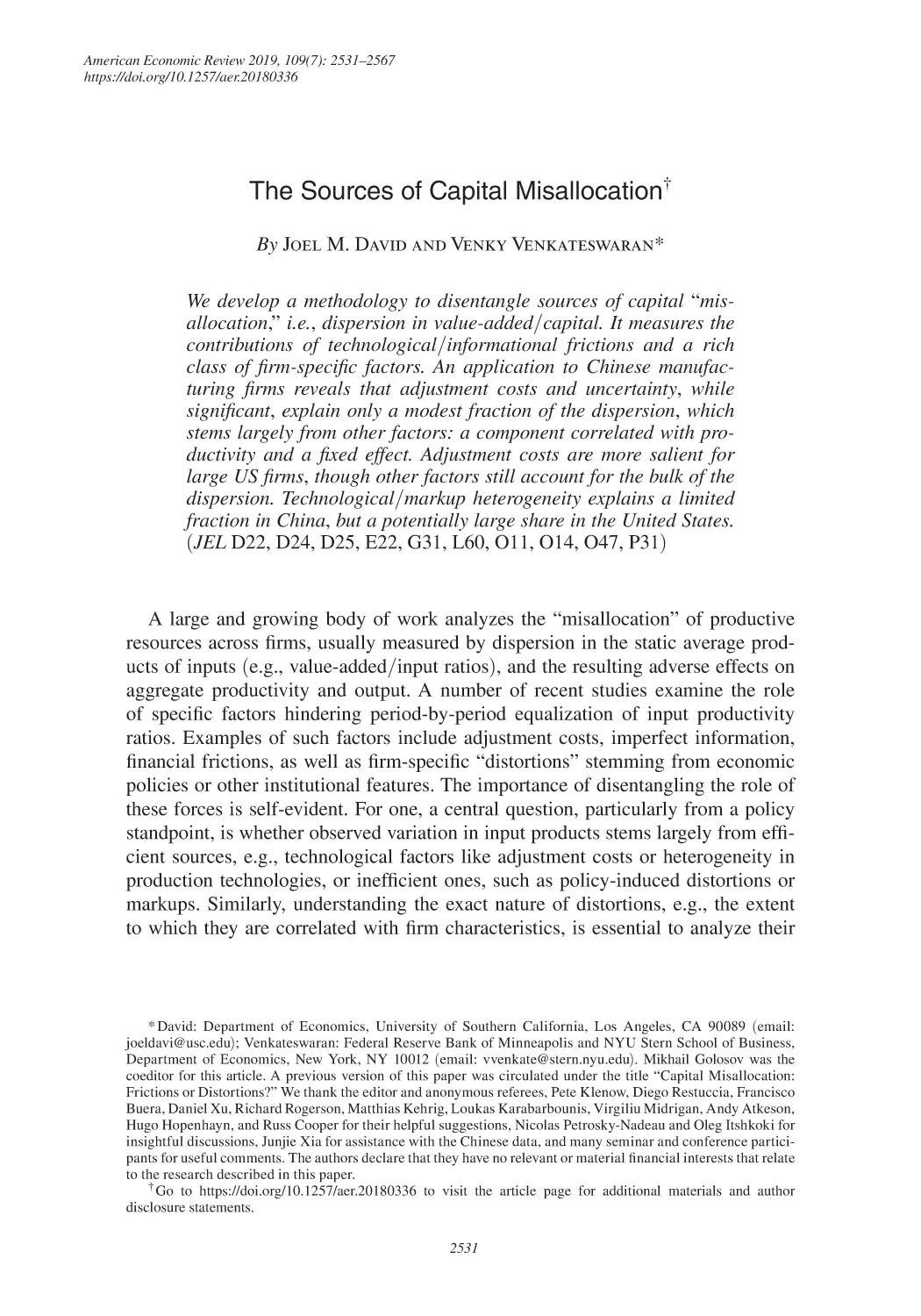
Panel A of Figure 1 shows how these properties help identify the two parameters.
The panel plots a pair of “isomoment” curves: each curve traces out combinations
of the two parameters that give rise to a given value of the relevant moment, holding the other parameters fixed. Take the ​​σ​  2k​  ​​curve: it slopes upward because higher​
ξ​and lower ​γ​ have similar effects on ​σ
​ ​  2k​  ​​; if ​γ​ is relatively small (in absolute value),
adjustment costs must be high in order to maintain a given level of ​​σ​ 2k​  ​​. Conversely, a
low ​ξ​ is consistent with a given value of ​σ
​ ​  2k​  ​​only if ​γ​ is very negative. An analogous
argument applies to the ​​ρk​,​k−​ 1​​​​​isomoment curve: since higher ​ξ​ and more negative​
γ​have opposite effects on ​​ρ​k,​k−​ 1​​​,​​ the curve slopes downward. As a result, the two
curves cross only once, yielding the unique combination of the parameters that is
consistent with both moments. By plotting curves corresponding to the empirical
values of these moments, we can uniquely pin down the pair ​(​ ξ, γ)​​ (holding all other
parameters fixed).
The graph also illustrates the potential bias introduced when examining these
forces in isolation. For example, estimating adjustment costs while ignoring
­correlated distortions (i.e., imposing ​γ = 0​) puts the estimate on the very ­right-hand
16

The latter is true only for ​γ > −1​, which is the empirically relevant region.

2544

JULY 2019

THE AMERICAN ECONOMIC REVIEW

Panel A. Adjustment costs
versus correlated distortions
2.2
2
1.8

Panel B. Uncertainty versus correlated distortions
0.08

σ k2
ρk,k−1

λarpk,a

0.06

V

1.6

ξ

ρk,a−1

1.4
1.2

0.04
0.02

1
0.8
−0.4

−0.35

γ

−0.3

Panel C. Transitory versus correlated distortions
0.15

0
−0.6

−0.25

0.08

λarpk,a
ρk,k−1

−0.3

γ

−0.2

−0.1

0

ρk,a−1
ρk,k−1

0.06

2

V

σε
0.05

−0.6

−0.4

Panel D. Uncertainty versus adjustment costs

0.1

0

−0.5

0.04
0.02

−0.5

−0.4

−0.3

γ

−0.2

−0.1

0
0

0.5

1

ξ

1.5

2

Figure 1. Pairwise Identification: Isomoment Curves

side of the horizontal axis. The estimate for ​ξ​ can be read off the vertical height of
the isomoment curve corresponding to the targeted moment. Because the ​​σ​  2k​  ​​ curve
is upward sloping, targeting this moment alone leads to an overestimate of adjustment costs (at the very right of the horizontal axis, the curve is above the point of
­intersection, which corresponds to the true value of the parameters).17 Targeting​​
​ k​,​k−1
ρ​k,​k−1
​ ​​​​​alone leads to a bias in the opposite direction: since the ​ρ
​ ​​​​​curve is downward sloping, imposing ​γ = 0​yields an underestimate of adjustment costs.
The remaining panels in Figure 1 repeat this analysis for other combinations of
parameters. Each relies on the same logic as shown in panel A.
Uncertainty and Correlated Distortions.—To disentangle information frictions
from correlated factors (panel B), we use the correlation of investment with past
,​​ and the regression coefficient ​
​λarpk,a
​ ​​​. These
innovations in productivity, ​
​ρk​,​a−​ 1​​​
moments can be written as
​σμ​ ​​ ​ψ2​​​​(1 + γ)​
​  V2  ​​(1 − ​ψ​1​​)​ + ​ψ​1​​ _
​​   
​,
(12)	​
​ρk​,​a−​ 1​​ ​​ = ​ _
​σk​ ​
​​
[ ​σ​  μ​​ 
]
(13)

17

V  ​ ​.​
​​λarpk,a
​ ​​  = 1 − ​(1 − α)​​(1 + γ)​​ψ2​​​​ 1 − ​ _
​σ​  2μ​​  )
(

This approach would also predict a counterfactually high level of the autocorrelation of investment.

VOL. 109 NO. 7

DAVID AND VENKATESWARAN: THE SOURCES OF CAPITAL MISALLOCATION

2545

A higher V
​ ​implies a higher correlation of investment with lagged productivity innovations. Intuitively, the more uncertain is the firm, the greater the tendency for its
actions to reflect productivity with a one-period lag. In contrast, a higher (more
­negative) ​γ​ increases the relative importance of transitory factors in the firm’s investment decision, reducing its correlation with productivity. Therefore, to maintain a
​ ​must be accompanied by a less negative γ
​ ​, i.e.,
given level of ​​ρk​ ,​a−​ 1​​​,​​ a decrease in V
the isomoment curve slopes downward. On the other hand, higher uncertainty and
a more negative gamma both cause a​ rpk​to covary more positively with contemporaneous productivity, ​a​, leading to an upward sloping ​​λa​ rpk,a​​​curve. Together, these
two curves pin down ​V​and ​γ​, holding other parameters fixed.
As before, the graph also reveals the direction of bias when estimating these factors in isolation. Assuming full information (​V = 0​) and using ​λ
​ a​rpk,a​​​to discipline
the strength of correlated distortions, for example, as in Bartelsman, Haltiwanger,
and Scarpetta (2013) and Buera and Fattal-Jaef (2018), overstates their importance.
Using the lagged responsiveness to productivity to discipline information frictions
while abstracting from correlated factors understates uncertainty.
Transitory and Correlated Distortions.—To disentangle correlated and uncorrelated factors, consider ​λ
​ a​rpk,a​​​and ​​ρk​,​k−1
​ ​​​​​. The former is increasing in the severity of
correlated distortions, but independent of transitory ones, implying a vertical isomoment curve. The latter is decreasing in both types of distortions: a more negative ​γ​
and higher ​​σ​  2ε​ ​​both increase the importance of the transitory determinants of investment, yielding an upward sloping isomoment curve.
Uncertainty and Adjustment Costs.—Finally, panel D shows the intuition for disentangling uncertainty from adjustment costs. An increase in the severity of either
of these factors contributes to sluggishness in the response of actions to productivity, i.e., raises the correlation of investment with past productivity shocks ​​ρ​k,​a−1
​ ​​​​​.
​
​​
is
independent
of
uncertainty
and
However, the autocorrelation of investment ​ρ
​ ​k,​k−1
​ ​​
determined only by adjustment costs (and other factors). Thus, holding those other
factors fixed, the two moments, ​​ρk​,​a−1
​ ​​​​​and ​​ρ​k,​k−1
​ ​​​​​, jointly pin down the magnitude of
adjustment frictions and the extent of uncertainty.
III. Quantitative Analysis

The analytical results in the previous section showed a tight relationship between
​ a−​ 1​​,​​  ​ρ​k,​k−​ 1​​,​​  ​σ​  2k​  ​, ​λarpk,a
​ ​​)​​and the parameters ​​(V, ξ, ​σ​  2ε​ ​, γ)​​for the special
the moments ​​(​ρk,​
case of ​ρ = 1​. In this section, we use this insight to develop an empirical strategy
for the more general case where productivity follows a stationary AR(1) process
and apply it to data on Chinese manufacturing firms. This allows us to quantify the
severity of the various forces and their impact on ​arpk​dispersion and economic
aggregates. For purposes of comparison, we also provide results for publicly traded
firms in the United States.18 In Section IV, we extend our methodology to explore
18
The two sets of firms are not directly comparable due to their differing coverage. For example, the Chinese
data include many more small firms. Similarly, there may be selection biases when using data on publicly traded
firms. To partly address this concern, in online Appendix J, we repeat the analysis on Chinese publicly traded

2546

THE AMERICAN ECONOMIC REVIEW

JULY 2019

some specific candidates for firm-specific factors other than adjustment/informational frictions.
A. Parameterization
We begin by assigning values to the more standard preference and production
parameters of our model. We assume a period length of one year and accordingly
set the discount factor β
​ = 0.95​. We use an annual depreciation rate of δ​ = 0.10​.
We keep the elasticity of substitution ​θ​common across countries and set its value
to 6, roughly in the middle of the range of values in the literature.19 We assume
constant returns to scale in production, but allow the parameters ​​​αˆ ​​1​​​and ​​​αˆ ​​2​​​to vary
across countries. In the United States, we set these to standard values of 0.33 and
0.67, respectively, which implies ​α = 0.62​.20 For China, we set a higher capital
share, namely, ​​​αˆ ​​1​​  = ​​αˆ ​2​​​  = 0.5​, in line with evidence from a number of recent
papers, for example, Bai, Hsieh, and Qian (2006). These values imply an ​α​ equal to
0.71 in China.21
Next, we turn to the parameters of the productivity process, ​​ai​t​​​: the persistence,​
ρ​, and the variance of the innovations, ​σ
​ ​  2μ​​.​  Under our assumptions, firm-level productivity is directly given by (up to an additive constant) ​​ai​t​​  = v​ai​t​​  − α​k​it​​​ where
​v​ai​t​​​denotes the log of value-added.22 Controlling for industry-year fixed effects to
isolate the firm-specific component, we use a standard autoregression to estimate the
parameters ​ρ​ and ​​σ​  2μ​​.​ 
To pin down the remaining parameters (the adjustment cost, ​ξ​, the quality
of information, ​V​, and the size of other factors, ​γ​and ​​σ​  2ε​ ​​) we follow a strategy
informed by the results in the previous section. Specifically, we target the correlation of investment growth with lagged innovations in productivity (​​ρ​ι,​a−1
​ ​​​)
​​ , the auto2
correlation of investment growth (​​ρι​,​ι−1
​ ​​​​​), the variance of investment growth (​​σ​  ι​  ​​)
and the correlation of the average product of capital with productivity (​​ρ​arpk,a​​)​.23
Finally, to infer ​σ
​ ​  2χ​​,​  the variance of the fixed component in (6), we match the overall
​ ​  2χ​​.​ 
dispersion in the average product of capital, ​σ
​ ​  2arpk​​, which is clearly increasing in ​σ
firms. We find patterns that are quite similar to those for Chinese manufacturing firms, suggesting that cross-country differences in frictions and distortionary factors are quite significant. This conclusion is further supported by
results for two additional countries, Colombia and Mexico, also presented in online Appendix J.
19
In online Appendix I.3, we report results for ​θ = 3​, the value used in Hsieh and Klenow (2009).
20
This is very close to the estimate of 0.59 in Cooper and Haltiwanger (2006). We also estimated ​α​following
the indirect inference approach in, e.g., Cooper, Gong, and Yan (2015). Specifically, we find the value of α
​ ​so that
the coefficient from an ordinary least squares (OLS) regression of value-added on capital using model-simulated
data matches its counterpart from an identical regression in the data. This procedure also yields ​α = 0.62​.
21
Using the same capital share for both countries yields a very similar decomposition of observed ​​σ​2arpk​​. More
generally, the curvature of the profit function, ​α​, plays a key role in determining the TFP/output implications of a
given degree of ​σ
​ ​2arpk​​, but does not materially change the estimated contributions of various factors, the main focus
of this paper. See also Section VB (where labor distortions leads to a higher α
​ )​ , online Appendix I.3 (where a lower
elasticity of substitution leads to a lower ​α​), as well as Section VD (sectoral heterogeneity in ​α​).
22
An alternative strategy is to measure the true productivity directly, i.e., ​a​ˆ i​t​ = v​ai​t​− ​α​1​​ki​t​− ​α​2​​n​it​​, and construct the implied ​a​ i​t​ = _
​1 −1 ​α​​​​aˆ i​t​​. The two approaches are equivalent under an undistorted labor choice, but online
2
Appendix E.1 shows that more generally, firm-specific capital profitability, ​a​ i​t​​, is a combination of productivity and
a labor distortion. As a result, inferring ​​ai​t​​from ​​aˆ ​it​​without adjusting for a potentially distorted labor choice can lead
to biased estimates, while the strategy of directly measuring ​​ai​t​​, as we do here, remains valid.
23
We use investment growth to partly cleanse the data of firm-level fixed effects, which have been shown to play
a significant role in firm-level investment data (in the analytical cases studied earlier, we used the level of investment). See Morck, Shleifer, and Vishny (1990) for more on this issue. Online Appendix I.4 shows that our results
are largely unchanged if we use the autocorrelation and variance of investment in levels, rather than growth rates.

VOL. 109 NO. 7

DAVID AND VENKATESWARAN: THE SOURCES OF CAPITAL MISALLOCATION

2547

Table 1—Parameterization: Summary
Parameter
Preferences/production
​θ​
​β​
​δ​
​​​αˆ ​​1​​​
​​​αˆ ​​2​​​
Productivity/frictions
​ρ​
​​σ​  2μ​​​ 
​​
V
​ξ​
​γ​
​​σ​  2ε​ ​​
​​σ​  2χ​​​ 

Description

Target/value

Elasticity of substitution
Discount rate
Depreciation
Capital share
Labor share

6
0.95
0.10
0.33 US/0.50 China
0.67 US/0.50 China

Persistence of productivity
Shocks to productivity
Signal precision
Adjustment costs
Correlated factors
Transitory factors
Permanent factors

}

}

​​ρ​a,​a​−1​​​​​
​​σ​  2a​​​ 

​ ​ι,​a​−1​​​​​
​ρ
​​ρ​ι,​ι−1
​ ​​​​​
​​ρarpk,a
​ ​​​
​​σ​  2ι​  ​​
​​σ​  2arpk​​

Thus, by construction, our parameterized model will match the observed ​arpk​ dispersion in the data, allowing us to decompose the contribution of each factor. Online
Appendix C describes our numerical estimation procedure in detail. We summarize
our empirical approach in Table 1.
B. Data
The data on Chinese manufacturing firms are from the Annual Surveys of
Industrial Production conducted by the National Bureau of Statistics. The surveys
include all industrial firms (both state-owned and non-state-owned) with sales above
5 million RMB (about $600,000). We use data spanning the period 1998–2009.24
The original data come as a repeated cross section. A panel is constructed following
almost directly the method outlined in Brandt, Van Biesebroeck, and Zhang (2014),
which also contains an excellent overview of the data for the interested reader. The
Chinese data have been used multiple times and are by now familiar in the misallocation literature (for example, Hsieh and Klenow 2009) although our use of the
panel dimension is rather new. The data on United States publicly traded firms come
from Compustat North America. We use data covering the same period as for the
Chinese firms.
We measure the firm’s capital stock, ​k​ ​it​​​, in each period as the value of fixed
assets in China and of property, plant and equipment (PP&E) in the United States.25
Value-added is estimated as a constant fraction of revenues using a share of intermediates of 0.5. We measure the average product of capital as a​ rp​ki​t​​  = v​ait​ ​​  − ​k​it​​​.
24
Industrial firms correspond to Chinese Industrial Classification codes 0610-1220, 1311-4392, and 4411-4620,
which includes mining, manufacturing, and utilities. Early vintages of the NBS data did not report all variables for
the full set of firms in the years after 2007. Although this does not seem to be an issue in our sample (all the variables we use are well populated in all years), we have also redone our analysis using data only through 2007. The
estimates are very similar (as noted below, the moments are fairly stable over time).
25
Our baseline measure of the capital stock uses reported book values. In Section VD (details in online
Appendix I.5), we construct the capital stock using the perpetual inventory method for the US firms and reestimate
the model. This yields slightly different point estimates, but very similar patterns for the role of various factors.

2548

JULY 2019

THE AMERICAN ECONOMIC REVIEW

Table 2—Target Moments

China
United States

​ρ​

​​σ​  2μ​​​ 

​​ρ​ι,​a​−1​​​​​

​0.91​
​0.93​

​0.15​
​0.08​

​0.29​
​0.13​

​​ρ​ι,​ι−​ 1​​​​​

​ 0.36​
−
​− 0.30​

​​ρarpk,a
​ ​​​

​​σ​  2ι​  ​​

​​σ​ 2arpk​​

​0.76​
​0.55​

​0.14​
​0.06​

​0.92​
​0.45​

Net investment and productivity growth are obtained by first differencing ​​k​it​​​ and​​
a​it​​​, respectively. To isolate the firm-specific variation in our data series, we extract
a time-by-industry fixed effect from each and use the residual. In both countries,
industries are classified at the four-digit level. This is equivalent to deviating each
firm from the unweighted average within its industry in each period and also eliminates aggregate components. After eliminating duplicates and problematic observations (for example, firms reporting in foreign currencies), outliers, observations with
missing data, etc., our final sample consists of 797,047 firm-year observations in
China and 34,260 in the United States. Online Appendix B provides further details
on how we build our sample and construct the moments, as well as summary statistics from 2009.26
Table 2 reports the target moments for both countries.27 The first two columns
show the productivity moments, which have similar persistence but higher volatility
in China. The remaining columns show that, in China, investment growth is more
correlated with past shocks, more volatile and less autocorrelated. The Chinese
data also show a higher correlation between productivity and a​ rpk​and substantially
larger dispersion in a​ rpk​. These patterns will lead us to significantly different estimates of the severity of various factors across the two sets of firms.
C. Identification
Before turning to the estimation results, we revisit the issue of identification.
Although we no longer have analytical expressions for the mapping between
moments and parameters, we use a numerical experiment to show that the intuition
developed in Section II for the random walk case applies here as well. In that section, we used a pairwise analysis to demonstrate how various moments combine
to help disentangle the sources of observed ​arpk​dispersion. Here, we repeat that
analysis by plotting numeric isomoment curves in Figure 2, using the moments and
parameter values for US firms (from Tables 2 and 3, respectively). They reveal the
same patterns as Figure 1, indicating that the logic of that special case goes through
here as well.28

26

We have also examined the moments year-by-year. They are reasonably stable over time.
We report bootstrapped standard errors for the moments in online Appendix Table C.1. Given the large sample sizes (almost 800,000 in China and 35,000 in the United States), the estimates of the moments are extremely
precise.
28
The differences in the precise shape of some of the curves in the two figures come partly from the departure
from the random walk case and also from the fact that they use slightly different moments (Figure 2 works with
changes in investment and ​​ρarpk,a
​ ​​while Figure 1 used changes in ​k​and ​λ
​ arpk,a
​ ​​).
27

VOL. 109 NO. 7

DAVID AND VENKATESWARAN: THE SOURCES OF CAPITAL MISALLOCATION

Panel A. Adjustment costs
versus correlated distortions
1.8

Panel B. Uncertainty versus correlated distortions
0.08

σ 2i
ρi,i −1

1.7
1.6

2549

ρi,a −1
ρarpk,a

0.06

ξ

V

1.5
1.4
1.3

0.04
0.02

1.2
1.1

−0.4

−0.35

−0.3

−0.25

γ

Panel C. Transitory versus correlated distortions
0.15

0

−0.2

−0.38

−0.36

−0.34

−0.32

γ

−0.3

−0.28

Panel D. Uncertainty versus adjustment costs
0.06

ρarpk,a
ρi,i −1

ρi,a −1
ρi,i −1

0.05
0.04

σe

2

V

0.1

0.05

0.03
0.02
0.01

0

−0.345

−0.34

−0.335

γ

−0.33

−0.325

0
1.3

1.35

ξ

1.4

1.45

Figure 2. Isomoment Curves: Quantitative Model

D. The Sources of Misallocation
Table 3 contains our baseline results. In the top panel we display the parameter
estimates.29 In the second panel of Table 3, we report the contribution of each factor to ​arpk​dispersion, which we denote Δ
​ ​σ​2arpk​​.30 These are calculated under the
assumption that only the factor of interest is operational, i.e., in the absence of the
others, so that the contribution of each one is measured relative to the undistorted
first-best.31 The third panel expresses this contribution as a percentage of the total​
arpk​dispersion measured in the data, denoted ​Δ​σ​  2arpk​/​ ​σ​  2arpk​​. Because of interactions
between the factors, there is no a priori reason to expect these relative contributions
to sum to 1. In practice, however, we find that the total is reasonably close to 1,
allowing us to interpret this exercise as a decomposition of total observed dispersion. In the bottom panel of the table, we compute the implied losses in aggregate
29
Online Appendix Table C.1 reports standard errors and compares the model-simulated moments (at the estimated parameters) to their empirical counterparts. The parameters are quite precisely estimated (again, both of our
firm-level datasets have a relatively large number of observations) and the model matches the five moments almost
exactly in both countries.
30
For adjustment costs, we do not have an analytic mapping between the severity of these costs and ​σ
​ ​2arpk​​, but
this is a straightforward calculation to make numerically; for each of the other factors, we can compute their contributions to a​ rpk​dispersion analytically.
31
An alternative would be to calculate the contribution of each factor holding the others constant at their estimated values. It turns out that the interactions between the factors are small at the estimated parameter values, so
the two approaches yield similar results. Online Appendix Table D.1 shows that the effects of each factor on a​ rpk​
dispersion in the United States are close under either approach. Interaction effects are even smaller in China.

2550

JULY 2019

THE AMERICAN ECONOMIC REVIEW

Table 3—Contributions to “Misallocation”
Adjustment costs
Parameters
China
United States

ξ​ ​
​0.13​
​1.38​

​Δσ
​ ​  2arpk​​
China
United States

Uncertainty

Correlated

​​
V
​0.10​
​0.03​

​​
γ
​− 0.70​
​− 0.33​

​0.01​
​0.05​

​0.10​
​0.03​

China
United States

​1.3%​
​10.8%​

​ a​
Δ
China
United States

​0.01​
​0.02​

​Δ​σ​  2arpk​/​ ​σ​  2arpk​​

Other factors
Transitory Permanent
​ ​  2ε​ ​​
​σ
​0.00​
​0.03​

​ ​  2χ​​​ 
​σ
​0.41​
​0.29​

​0.44​
​0.06​

​0.00​
​0.03​

​0.41​
​0.29​

​10.3%​
​7.3%​

​47.4%​
​14.4%​

​0.0%​
​6.3%​

​44.4%​
​64.7%​

​0.08​
​0.01​

​0.38​
​0.03​

​0.00​
​0.01​

​0.36​
​0.13​

TFP, again relative to the undistorted first-best level, i.e., Δ
​ a = ​a​​  ∗​  − a​. Once we
have the contribution of each factor to a​ rpk​dispersion, computing these values is
simply an application of expression (9).
Adjustment Costs.—Our results show evidence of economically significant
adjustment frictions. For example, the estimate of 1.38 for ​ξ​in the United States
implies a value of 0​ .2​for ​ξ​ˆ ​​in the adjustment cost function.32 This puts us in the
middle of previous estimates of convex costs in the literature, though differences
in data and empirical strategies complicate direct comparisons. For example, using
US manufacturing data, Asker, Collard-Wexler, and De Loecker (2014) estimate a
convex adjustment cost of 8.8 in a monthly model, which translates to an annual​​
ξˆ ​ = 0.73​, roughly a factor of four above our estimate.33 Our estimate is closer to,
and slightly higher than, Cooper and Haltiwanger (2006), who find ​ξ​ˆ ​ = 0.05​ for
US manufacturing plants.
What leads us to find different estimates? The answer lies primarily in the fact
that our model explicitly includes additional factors that may act on the investment
decision (e.g., distortions) and consequently, our empirical strategy is designed
to match a broader set of moments.34 The papers mentioned above abstract from
these factors and focus on matching different moments. For example, Asker,
­Collard-Wexler, and De Loecker (2014) target the variability of investment (among
The mapping between ​ξ​and ​​ξˆ ​​is in equation (A.1) in online Appendix A.1.
To interpret this difference, a firm that doubles its capital stock in a year would incur an adjustment cost
equal to 11 percent of the value of the investment according to our estimate, but equal to 60 percent at the Asker,
­Collard-Wexler, and De Loecker (2014) estimate.
34
There are a few other differences between our approach and these papers: (i) they have convex and n­ onconvex
(fixed) adjustment costs. In Section VA, we show that our estimates of ​ξ​ˆ ​​change little when we introduce a fixed
cost; (ii) they use moments of investment in levels while we work with growth rates. In online Appendix I.4,
we show that targeting the variance and autocorrelation of investment in levels changes the estimate of ​ξ​ˆ ​​ only
slightly; (iii) Asker, Collard-Wexler, and De Loecker (2014) follow a different strategy to estimate the process for
profitability, ​a​ it​ ​​: they directly measure productivity ​a​ˆ it​ ​​and use the implied ​a​ ​it​​. See footnote 22. As we show in online
Appendix E.1, this strategy can overstate the volatility of ​​ait​ ​​, i.e., ​​σ​μ2​​, and bias adjustment cost estimates upward.
32
33

VOL. 109 NO. 7

DAVID AND VENKATESWARAN: THE SOURCES OF CAPITAL MISALLOCATION

2551

other moments), but do not try to match the autocorrelation, while Cooper and
Haltiwanger (2006) do the reverse. As we saw in Section II, in the presence of
correlated factors, the first strategy overstates the true extent of adjustment costs,
while the second understates it. It turns out that this bias can be quite large: an
adjustment cost-only model (i.e., ignoring other factors) estimated to match the
volatility of investment growth yields an estimate of ​ξ​ˆ ​​about 60 percent higher
than our baseline estimate, but predicts a counterfactually high autocorrelation of
investment growth: ​− 0.17​versus ​− 0.30​in the data. A strategy targeting only the
serial correlation leads to the opposite conclusion: a lower estimate of ​​ξˆ ​​, but at the
cost of excessively high variability compared to the data. These patterns are exactly
in line with the arguments developed in Section II. More broadly, these exercises
can partly explain the wide range of adjustment cost estimates in the literature: when
adjustment costs are estimated without explicitly controlling for other factors, the
results can be quite sensitive to the particular moments chosen.35 Indeed, our results
suggest that explicitly accounting for these additional factors is essential in order to
reconcile a broad set of moments in firm-level investment dynamics.
The estimated value of ξ​ ​is lower in China. Investment growth in China is both
more volatile and less serially correlated than for US firms, which (together with the
other moments) leads the estimation to find a lower degree of adjustment frictions.
Importantly, as in the United States, one would reach a very different conclusion
from examining a model with only adjustment costs: for example, estimating such
a model by targeting ​​σ​  2ι​  ​​in China yields an estimate for ​ξ​ of about 1.5, roughly 10
times larger than the one in Table 3.
Perhaps most importantly for purposes of our analysis, in both countries, the estimated adjustment costs do not contribute significantly to a​ rpk​dispersion. If adjustment costs were the only friction in China, ​​σ​ 2arpk​​ would be ​0.01​ (the observed level is​
0.92​). The higher estimate of ​ξ​ in the United States implies a slightly higher, though
still modest, contribution (by themselves, adjustment costs lead to ​​σ​ 2arpk​ ​ = 0.05​ or
11 percent of the observed dispersion). The corresponding aggregate TFP losses are
1 and 2 percent in the two countries, respectively.
This does not mean that adjustment costs are irrelevant for understanding firmlevel investment dynamics. Setting adjustment costs to zero in the United States
while holding the other parameters at their estimated values causes the variance of
investment growth to spike to ​1.68​(compared to ​0.06​in the data) and the autocorrelation to plummet to −
​ 0.62​ (data: ​− 0.30​). However, ​σ
​ ​  2arpk​​falls only modestly,
from 0​ .45​to ​0.41​. Reestimating the model without adjustment costs (and dropping
the autocorrelation as a target) also leads to a counterfactually low autocorrelation
(​− 0.50​).36 In other words, while adjustment frictions are an important determinant
of investment dynamics, they do not generate significant dispersion in average products of capital.37

Bloom (2009) points out the wide variation in these estimates, ranging from 0 to 20 (Table IV).
The estimates for other parameters also change: notably, a more negative ​γ​is needed to match ​σ
​ ​2ι​​​.
37
Asker, Collard-Wexler, and De Loecker (2014) make a similar observation: across various specifications of
adjustment costs (including one with zero adjustment costs and a one-period time-to-build), their model’s performance in capturing dispersion in a​ rpk​is not dramatically altered, even though the implications for other moments
(e.g., the variability of investment) are quite different. See Table 9 and the accompanying discussion in that paper.
35
36

2552

THE AMERICAN ECONOMIC REVIEW

JULY 2019

Uncertainty.—Table 3 shows that firms in both countries make investment decisions under considerable uncertainty, with the information friction more severe for
Chinese firms. As a share of the prior uncertainty, ​​σ​  2μ​​,​  residual uncertainty, ​V/​σ​  2μ​​,​  is​
0.42​in the United States and ​0.63​in China.38 In an environment where imperfect
information is the only friction, we have ​σ
​ ​  2arpk​ ​ = V​, so the contribution of uncertainty alone to observed ​arpk​dispersion can be directly read off the second column
in Table 3, namely ​0.10​in China and ​0.03​in the United States. These represent
about 10 and 7 percent of total ​arpk​dispersion in the two countries, respectively.
The implications for aggregate TFP are substantial in China (losses are about 8 percent) and are lower in the United States, about 1 percent. Note, however, that imposing a one-period time-to-build assumption where firms install capital in advance
without any additional information about innovations in productivity, i.e., setting ​V
= ​σ​  2μ​​,​  would overstate uncertainty (and bias the estimates of adjustment costs and
other parameters). Indeed, doing so yields estimates of V
​ ​that are about 55 percent
higher in China and a factor of 2.5 times higher in the United States.
Distortions.—The last three columns of Table 3 show that other, potentially distortionary, factors play a significant role in generating the observed a​ rpk​dispersion in
both countries. Turning first to the correlated component, the negative values of ​γ​ suggest that they act to disincentivize investment by more productive firms and especially
so in China. The contribution of these distortions to ​arpk​dispersion is given by ​​γ​​  2​ ​σ​  2a​​,​ 
which amounts to 0​ .44​in China, or 47 percent of total dispersion. The associated
aggregate consequences are also quite sizable: TFP losses from these sources are
38 percent. In contrast, the estimate of ​γ​in the United States is significantly less negative than in China, suggesting that these types of correlated factors are less of an issue
for firms in the United States, both in an absolute sense (the ​arpk​dispersion from these
factors in the United States is 0​ .06​, less than o­ ne-seventh that in China) and in relative
terms (they account for only 14 percent of total observed ​arpk​dispersion in the United
States). The corresponding TFP effects are also considerably smaller for the United
States: losses from correlated sources are only about 3 percent.
Next, we consider the role of distortions that are uncorrelated with firm productivity. Table 3 shows that purely transitory factors (measured by ​σ
​ ​  ε2​  ​​) are negligible in
both countries, but permanent firm-specific factors (measured by ​σ
​ ​  2χ​​)​  play a prominent role. Their contribution to a​ rpk​dispersion, which is also given by ​σ
​ ​  2χ​​,​  amounts
to ​0.41​in China and ​0.29​in the United States. Thus, their absolute magnitude in
the United States is considerably below that in China, but in relative terms, these
factors seem to account for a substantial portion of measured ​arpk​dispersion in
both ­countries. The aggregate consequences of these types of distortions are also

38
Our values for ​V/​σ​2μ​​are similar to those in David, Hopenhayn, and Venkateswaran (2016), who find 0.41
and 0.63 for publicly traded firms in the United States and China, respectively. The estimates of V are different but
are not directly comparable: David, Hopenhayn, and Venkateswaran (2016) focus on longer time horizons (they
analyze 3-year time intervals). This might lead one to conclude that ignoring other factors, as David, Hopenhayn,
and Venkateswaran (2016) do, leads to negligible bias in the estimate of uncertainty. But, this is not a general result
and rests on the fact that adjustment costs and uncorrelated distortions are estimated to be modest. Then, as Figure 2
shows, the sensitivity of actions to signals turns out to be a very good indicator of uncertainty. If, on the other hand,
adjustment costs and/or uncorrelated factors were much larger, the bias from estimating uncertainty alone can be
quite significant.

VOL. 109 NO. 7

DAVID AND VENKATESWARAN: THE SOURCES OF CAPITAL MISALLOCATION

2553

s­ignificant, with TFP losses of 36 percent in China and about 13 percent in the
United States.
In sum, the estimation results point to the presence of substantial distortions to
investment, especially in China, where they disproportionately disincentivize investment by more productive firms. Section V and online Appendix I show that these
results are robust to a number of modifications to our baseline setup, e.g., allowing
for nonconvex adjustment costs, a frictional labor choice, richer stochastic processes
on productivity and distortions, curvature assumptions and additive measurement
error. Further, we have applied the methodology to data on Colombian and Mexican
firms (in addition to the set of publicly traded firms in China): the results resemble
those for Chinese manufacturing firms, in that they point to a substantial role for
correlated factors, as well as fixed ones (details are in online Appendix J).
What patterns in the data lead us to this conclusion? In both countries, we see
considerable dispersion in ​arpk​, which tends to be correlated with firm productivity.
The fact that investment growth is not very correlated through time and responds
only modestly to past shocks limits the role of adjustment and informational frictions and assigns a substantial role to other factors. The high correlation of ​arpk​ with
productivity, particularly in China, suggests that these factors vary systematically
with productivity. In both countries, large fixed distortions, uncorrelated with productivity, are necessary to rationalize the total observed dispersion in a​ rpk​. In the
next section, we explore some candidates for these firm-specific factors.
IV. Firm-Specific Factors: Some Candidates

Our results suggest a large role for firm-specific “distortions” in explaining
the observed a​ rpk​dispersion. In this section, we extend our baseline framework
and empirical methodology to investigate three potential sources: heterogeneity
in markups and production technologies, size-dependent policies and financial
considerations.
A. Heterogeneity in Markups and Technologies
In our baseline setup, all firms within an industry (i) operated identical production
technologies and (ii) were monopolistically competitive facing CES demand curves
and therefore, had identical markups. As a result, any firm-level heterogeneity in
technologies and/or markups would show up in our estimates of other factors (note
also that this type of variation would drive a wedge between ​arpk​and the true marginal product of capital, implying that dispersion in the former is not necessarily a
sign of misallocation). Here, we explore this possibility using a modified version of
our baseline model. This requires more assumptions and additional data, but allows
us to provide an upper bound on the contribution of these elements.
We begin by generalizing the production function from Section I to include intermediate inputs and to allow for (potentially time-varying) heterogeneity in input
intensities. Specifically, the output of firm ​i​is now given by
​ˆ ​​ ​​
​α

​ζ​ˆ ​​ ​​−​​αˆ ​​ ​​

1−​​ζˆ ​​ ​​

	​
​Y​it​​  = ​K​  it​  it​​N​  iti​  t it​​M​  it​  it​,​

2554

THE AMERICAN ECONOMIC REVIEW

JULY 2019

where ​M
​ ​it​​​denotes intermediate or materials input. The price of these inputs, potentially firm-specific, is denoted ​​P​  M
it​  ​​. Throughout this section, we abstract from adjustment/information frictions in firms’ input decisions. This is largely for simplicity,
but is also supported by the relatively modest role played by these dynamic considerations in our baseline estimates.39
Capital and labor choices are assumed to be subject to a factor-specific “distor​ ​  Nit​  ​​, respectively, but the choice of
tion” (in addition to the markup), denoted ​​T​  Kit​  ​​and ​T
intermediates is undistorted except for the markup. Since the method remains valid
even with unobserved firm-specific variation in the price of intermediate goods,
it does allow for distortions in the market for intermediate inputs, so long as they
are reflected in prices. Formally, these assumptions imply that the firm’s optimal
choices solve the following cost minimization problem:
	​​  min​ ​​ ​Rt​​​ ​T​  Kit​  ​ ​Ki​t​​  + ​W​t​​ ​T​  Nit​  ​ ​Ni​t​​  + ​P​  M
it​  ​ ​Mi​t​​,
​Kit​ ​​,​Nit​ ​​,​Mit​ ​​

subject to
​​αˆ ​​ ​​

​​ζˆ ​​ ​​−​​αˆ ​​ ​​

1−​​ζˆ ​​ ​​

	​
Yi​t​​  ≤ ​K​  it​  it​ ​N​  iti​  t it​ ​M​  it​  it​.​
The Contribution of Markup Dispersion.—To quantify the contribution of markup
dispersion, we use the powerful methodology of De Loecker and Warzynski (2012),
which allows us to measure firm-level markups without taking a stand on the nature
of competition/demand. To do so, we assume a common materials elasticity across
firms within an industry, i.e., ​​​ζˆ ​​it​​  = ​​ζˆ ​​t​​ ∀i​.40 Cost minimization then implies the following optimality condition (we suppress the time subscript on ​ζ​, though the method
remains valid with arbitrary time-variation):
​Y​it​​
M​Cit​ ​​
​P​  M​  ​​M​ ​​
ˆ _
​​   ​
 ​ ⇒ _
​  it it ​ = ​
,​
(14)	​
​P​  M
(1 − ​ζˆ ​)_
it​  ​  = M​Ci​t​​​(1 − ​ζ ​)​ ​ 
​Mi​t​​
​Pi​t​​​Yi​t​​
​Pi​t​​
where M
​ ​C​it​​​is the marginal cost of the firm. This condition states that, at the optimum, the firm sets the materials share of revenue equal to the inverse of the markup,​
M​Ci​t​​/​Pi​t​​​, multiplied by the materials elasticity ​1 − ​ζˆ ​​.
Expression (14) suggests a simple way to estimate the cross-sectional dispersion
in markups. The left-hand side is materials’ share of revenue: the within-industry
dispersion in this object (in logs) maps one-for-one into (log) markup dispersion.
Data on materials expenditures are directly reported in the Chinese data. In the
United States, we follow, e.g., De Loecker and Eeckhout (2017) and İmrohoroǧlu
and Tüzel (2014) and calculate intermediate expenditures as total expenses less
39
It is possible to extend the identification methodology from Section II to explicitly incorporate these forms
of heterogeneity. Although this would require more assumptions (e.g., on the correlation structure of m
­ arkups/
technologies with productivity and over time) and make the intuition more complicated, the basic insights should
still go through.
40
In online Appendix F, we allow the materials elasticity to vary across firms within an industry (our baseline
calculation already allows for variation across industries). Under certain orthogonality assumptions, we show that
the covariance of the materials share with ​arpk​and ​arpn​ (average product of labor) pins down the dispersion in
markups. This approach yields very similar (if slightly lower) estimates of markup dispersion in both countries.

VOL. 109 NO. 7

DAVID AND VENKATESWARAN: THE SOURCES OF CAPITAL MISALLOCATION

2555

labor expenses. The former are defined as sales less operating income and the latter
are imputed using number of employees and the average industry wage, from the
NBER-CES Manufacturing Industry Database.41
The results of applying this procedure are reported in Table 4. The variance of
the share of materials in revenue (the first row in the top panel) is about 0.06 in
the US Compustat data and 0.05 in China. This accounts for about 14 percent of
​​σ​  2arpk​​among the United States firms, but only about 4 percent among Chinese manufacturing firms. Thus, markup heterogeneity composes a nonnegligible fraction of
observed ​arpk​dispersion among United States publicly traded firms but seems to be
an almost negligible force in China.
Can markup variation help explain the large role for correlated distortions in
Section III? In theory, yes: markups that increase with size would be consistent with
the patterns uncovered in that section. Quantitatively, however, this does not seem to
hold much promise. In China, this is clear simply from the rather modest dispersion
in markups: the contribution of markups to ​arpk​dispersion is much smaller (0.05)
than the estimated total contribution of correlated factors (0.44). In the United
States, where dispersion in markups is more substantial, the data suggest they are
largely independent of firm size. For example, projecting the measured markup on
revenues yields a statistically significant, yet economically small, coefficient of 0.01
(the raw correlation between markups and revenues is 0.07).
The Contribution of Technology Dispersion.—Cost minimization also implies
that the average revenue products of capital and labor are given by42
​P​ ​​ ​Y​it​​
​Pit​ ​​
(15)	​
arp​ki​t​​  ≡ log​(_
​  it  ​
​  = log ​ _
 ​  − log ​​αˆ ​​it​​  + ​τ​  Kit​  ​  + Constant​,
​Ki​t​​ )
M​Ci​t​​

​P​ ​​ ​Yit​ ​​
​Pit​ ​​
​  it  ​
​  = log ​ _
 ​  − log​(​ζˆ ​  − ​​αˆ ​​it​​)​ + ​τ​  Nit​  ​  + Constant​
(16)	​
arp​n​it​​  ≡ log​(_
)
​Ni​t​​
M​Ci​t​​

–
​P​it​​
 ​ + ​ _____
​  ​α ​–  ​ ​log ​​αˆ ​​it​​  + ​τ​  Nit​  ​  + Constant,​
(17)	​
≈ log ​ _
M​Cit​ ​​ ( ​ζˆ ​ − ​α ​)

where ​​τ​  Kit​  ​​and ​​τ​  Nit​  ​​ denote (the logs of) the capital and labor wedges ​​T​  Kit​  ​​and ​​T​  Nit​  ​​, respectively, and α
​​– ​​is the average capital elasticity. Average revenue products are combinations of firm-specific production elasticities, markups and wedges. Note that the
capital elasticity, ​​α
​ˆ ​​it​​​, has opposing effects on the average products of capital and
labor: firms with a high ​​​αˆ ​​it​​​will, ceteris paribus, have a low ​arpk​and a high ​arpn​.
In other words, this form of heterogeneity acts like a “mix” distortion (as opposed
to “scale” factors, which distort all input decisions in the same direction). We will

41
Details of these calculations are provided in online Appendix B. In an earlier version of this paper, we also
used the reported wage bill, available for a smaller subset of firms. The results were broadly similar, though the
share of both markup and technology dispersion was somewhat higher (28 and 62 percent of ​​σ​2arpk​​for those firms).
–
42
See online Appendix F for details. The third equation is derived by log-linearizing (16) around ​​αˆ it​ ​ = ​α
​​.

2556

JULY 2019

THE AMERICAN ECONOMIC REVIEW

Table 4—Heterogeneous Markups and Technologies
China
Moments
​P​it​​ ​Yi​t​​
​​σ​​  2​​ log ​ _
 ​ ​​
M

(

​P​  t​  ​ ​Mi​t​​ )

​cov​(˜
​​arpk​it​ ​​, ​​˜
arpn​it​ ​​)​​
​ ​​  2​​(​​˜
​σ
arpk​it​ ​​)​​
​​σ​​  2​​(​​˜
arpn​it​ ​​)​​

Estimated ​Δ​σ​  2arpk​​
Dispersion in markups
Dispersion in ​log ​​αˆ ​​it​​​
Total

United States

0.05

0.06

0.41
1.37
0.76

0.23
0.52
0.35

0.05
0.30
0.35

(​3.8%​)
(​23.1%​)
(​26.9%​)

0.06
0.18
0.24

(​13.6%​)
(​44.4%​)
(​58.1%​)

Note: The values in parentheses in the bottom panel are the contributions to ​arpk​ dispersion
expressed as a fraction of total ​​σ​2arpk​​.

make use of this property to derive an upper bound for variation in ​​​αˆ ​​it​​​ using the
observed covariance of ​arpk​and ​arpn​. Let
​Pit​ ​​ ​Yit​ ​​
​P​it​​
_
˜
arpk​​
 ​ ​  − log​ _
	​
​​
it​​  ≡ log​(​ 
(​  M​Ci​t ​​​ )​​,
​Ki​t​​ )

​Pit​ ​​ ​Yit​ ​​
​P​it​​
_
	​
​​
arpn​​
 ​ ​  − log​ _
˜
it​​  ≡ log​(​ 
(​  M​Ci​t ​​​ )​​,
​Ni​t​​ )

denote the markup-adjusted average revenue products of capital and labor. Online
Appendix F proves the following result.
PROPOSITION 2: Suppose ​log​​αˆ ​i​t​​​is uncorrelated with the distortions τ​​ ​  Kit​  ​​and τ​​ ​  Nit​  ​​.
Then, the cross-sectional dispersion in ​log​​αˆ ​​it​​​ satisfies
​ ​  2​˜
σ
​ ​​σ​  2arpn​​ ​− cov​​(˜
​
arpk​
, ​˜
arpn​)​​​  ​
arpk​ ​˜
2
_________________________________
 ​.​
     
(18)	​
​σ​​  ​​(log ​​αˆ ​​it)​​ ​  ≤ ​     
2
–
–
​α
 ​
​α
 ​
2
2
____
˜
2 ​ ____
 ​
cov​
​
arpk​
,
 ​
arpn​
​ 
+ ​​
​ 
 ​
​​ 
​
 ​
​
σ
​ 
​ + ​
​
σ
​ 
˜
(
)
​
arpn​
˜​
–
arpk​
( ​ζˆ ​ − ​α– ​) ​˜
​ζˆ ​ − ​α
 ​
2

The bound in (18) is obtained by setting the correlation between ​τ​ ​  Kit​  ​​and ​τ​ ​  Nit​  ​​to 1.
​​
arpk​​
arpn​​it​​)​​, this maximizes the potenGiven the observed second moments of (​​ ˜
it​​, ​​˜
tial for variation in ​​α
​ˆ ​i​t​​​, which, as noted earlier, is a source of negative correlation
arpk​​
arpn​​it​​​. The expression for the bound reveals the main insight: the
between ˜
​​​
it​​​and ​​​˜
​​
arpk​​
arpn​​it)​​ ​​, the lower is the scope for hetmore positive the covariance between ​​(˜
it​​, ​​˜
erogeneity in ​​​αˆ ​​it​​​.
To compute this bound for the two countries, we set ​ζ​ˆ ​​, the share of materials in
gross output, to 0.5. The results, along with the moments used, are reported in Table
4. They show that heterogeneity in technologies can potentially account for a substantial portion of ​σ
​ ​  2arpk​​in the United States, as much as 44 percent, and a more modest, though still significant, fraction in China, about 23 percent.43 In other words, a
43

There is some evidence that the share of intermediates may be higher in China than the United States, see,
e.g., Table 1 in Brandt, Van Biesebroeck, and Zhang (2014). We recomputed the bound with ​ζ​ˆ​ = 0.25​and obtained

VOL. 109 NO. 7

DAVID AND VENKATESWARAN: THE SOURCES OF CAPITAL MISALLOCATION

2557

substantial portion of measured a​ rpk​dispersion in both countries may not be a sign
of misallocated resources at all. This is most striking in the United States, where the
average products of capital and labor covary less positively than in China.44
An alternative approach to assessing the potential for technology dispersion
is discussed in Hsieh and Klenow (2009), in which all the variation in firm-level
­capital-labor ratios is attributed to heterogeneity in ​​​αˆ ​​it​​​. This amounts to assuming
that ​τ​ ​  Kit​  ​ = ​τ​ Nit​  ​​, which implies
​ζˆ ​
 ​ log ​​αˆ ​​it​​  ⇒
	​
​ki​t​​  − ​n​it​​  = arp​nit​ ​​  − arp​k​it​​  ≈ ​ _____
–
​ζˆ ​ − ​α
 ​
( ​ζ ​ − ​α ​)

2

​ζ ​
	​
σ​​  2(​​ ​ki​t​​  − ​n​it)​​ ​  = ​​ ____
​  ˆ –  ​ ​​ ​ ​​σ​​  2​​(log ​​αˆ ​i​t​​)​.​
ˆ

This procedure yields estimates for ​​σ​​  2​​(log ​​αˆ ​​it​​)​​that are quite close to those in Table 4:
0.27 (compared to 0.30) for China and 0.16 (compared to 0.18) in the United States.
In sum, unobserved heterogeneity in markups and technologies seem to be promising candidates for firm-specific factors, which drive most of the ​arpk​ dispersion
in the data. This is particularly true for the United States, where they can explain as
much as 58 percent of the observed dispersion. In China, their role is more modest,
but still meaningful, at 27 percent.
B. Size-Dependent Policies
Our results show a significant role for factors correlated with firm-level productivity, especially in China, in explaining the observed variation in ​arpk​across firms.
Here, we show how policies that affect or restrict the size of firms can lead to a
correlated factor of this form. A number of papers have pointed out the prevalence
of distortionary size-dependent policies across a range of countries, for example,
Guner, Ventura, and Xu (2008). These policies often take the form of restrictions (or
additional costs) associated with acquiring capital and/or other inputs. To be clear,
our goal is not to explore the role of a particular policy in China or the United States.
Rather, we show how policies that are common in a number of countries can generate patterns that are, in a sense, isomorphic to factors correlated with productivity.
Toward this end, we generalize our baseline specification of firm-specific factors
in equation (6) to allow for a component that varies with the chosen level of capital.
Formally,
	​
​τ​it​​  = ​γ​k​​ ​kit​ ​​  + γ​a​it​​  + ​ε​it​​  + ​χ​i​​,​
where the parameter ​​γ​k​​​indexes the severity of this additional component. The
empirically relevant case is ​γ
​ ​k​​  < 0​, which implicitly penalizes larger firms. This
very similar results. We also verified the accuracy of the approximation by working directly with (16) instead of the
log-linearized version in (17). This yielded slightly lower bounds: 38 and 17 percent of ​σ​2arpk​​in the United States
and China, respectively.
44
In online Appendix F, we derive an analogous bound in the case with within-industry variation in the materials elasticity. The results are very similar.

2558

JULY 2019

THE AMERICAN ECONOMIC REVIEW

Table 5—Size versus Productivity-Dependent Factors
Correlated factors

​ + ​γ​k​​  = 0.71​ (baseline)
α
Parameters
​Δ​σ​  2arpk​/​ ​σ​  2arpk
 ​
​​

Size-dependent
​​γk​​​​

Prod.-dependent
​γ​

Total

Adj. costs
​ξ​

​0.00​
​0.0%​

​− 0.70​
​47.4%​

​47.4%​

​0.13​
​1.3%​

​ + ​γ​k​​  = 0.54​
α
Parameters
​Δ​σ​  2arpk​/​ ​σ​  2arpk​​

​− 0.18​
​14.2%​

​− 0.51​
​25.4%​

​39.6%​

​0.21​
​2.3%​

​ + ​γ​k​​  = 0.36​
α
Parameters
​Δ​σ​  2arpk​/​ ​σ​  2arpk​​

​− 0.36​
​29.6%​

​− 0.33​
​10.2%​

​39.8%​

​0.29​
​3.2%​

specification captures the essence of the policies discussed above in a tractable way
(e.g., it allows us to continue to use perturbation methods). With this formulation,
the log-linearized Euler equation takes the form
(19)  ​
​ki​t+1​​​(​(1 + β)​ξ + 1 − α − ​γ​k​​)​ 

= ​(1 + γ)​ ​E​it​​​[​a​it+1​​]​ + ​ε​it+1​​  + ​χ​i​​  + βξ​E​it​​​[​ki​t+2​​]​  + ξ​k​it​​.​

Expression (19) is identical to expression (4), but with ​α + ​γ​k​​​taking the place of ​α​.
It is straightforward to derive the firm’s investment policy function and verify that
the same adjustment goes through, i.e., expressions (7) and (8) hold, with α
​ ​ every​ k​ ​​​, changes
where replaced by ​α + ​γ​k​​​. Intuitively, the size-dependent component, ​γ
the effective degree of curvature in the firm’s investment problem; although the
curvature of the profit function remains ​α​, the firm acts as if it is ​α + ​γ​k​​​. If ​​γk​ ​​  < 0​,
the distortion dampens the responsiveness of investment to shocks. If ​γ
​ ​k​​  > 0​, the
responsiveness of investment is amplified.
Importantly, these effects are broadly similar to those coming from γ
​ ​: indeed,
if ​​γk​​​​were the only factor distorting investment choices, the implied law of motion
for ​​ki​t​​​is identical (up to a first-order) to one with only productivity-dependent fac​γ​k​​
_
 ​​. The implication of this isomorphism is that we cannot
tors, where ​γ = ​ 
1 − α − ​γk​​​
distinguish the two factors using observed series of capital and value-added alone.
This challenge also applies to the case when other factors are present, though the
mapping between the two is more complicated (and affects the other parameters as
well). We detail this mapping in online Appendix G.
What about the contribution to a​rpk​dispersion? Table 5 reports the results
for Chinese firms for two values of ​γ
​ k​​​​, namely −0.18 and −0.36 (these values
imply effective curvatures α
​ + ​γ​k​​​equal to one-quarter and one-half of the true ​α​,
respectively). The table shows two key results: first, a more negative ​​γk​​​​ reduces
the estimated ​γ​ (i.e., makes it less negative), suggesting that our baseline estimates
of correlated factors could be picking up such size-dependent policies. The total
contribution of both types of distortions is quite stable, ranging between 40 and

VOL. 109 NO. 7

DAVID AND VENKATESWARAN: THE SOURCES OF CAPITAL MISALLOCATION

2559

47 percent. Second, the estimates of adjustment costs remain modest over this wide
range of curvature.
C. Financial Frictions
In this section, we show that liquidity considerations can lead to size-dependent
distortions of the form analyzed in the previous subsection. We assume that firms
​ ​​, ​Bit+1
​ ​​)​​, where ​​Bit+1
​ ​​​denotes holdings of liquid assets, which
face a cost ​ϒ​(​Kit+1
earn an exogenous rate of return R
​ < 1/β​. The cost is increasing (decreasing)
in ​K
​ ​it+1​​​ (​​B​it+1​​​). This specification captures the idea that firms need costly liquidity
in order to operate (e.g., to meet working capital needs). Using a continuous penalty
function rather than an occasionally binding constraint allows us to continue using
perturbation methods. Note also that this differs from the standard borrowing constraint used widely in the literature on financial frictions. Our firms are not constrained
in terms of their ability to raise funds. This implies that self-financing, which often
significantly weakens the long-run bite of borrowing constraints, plays no role here.45
We use the following flexible functional form for the liquidity cost:
​ω​​​

​
​K​  1 ​
 ​,​
​  ​ωit+1
	​
ϒ​(​Ki​t+1​​, ​Bi​t+1)​​ ​  = ​νˆ ​  _
2​​​
​B​  it+1
 ​
​

where ​​νˆ ​​, ​​ω​1​​​, and ​​ω2​ ​​​are all positive parameters. The marginal liquidity cost of
capital, after optimizing over the choice of ​B
​ i​t+1​​​is given by (derivations in online
Appendix H)
​ω​​​
​ ​​, ​Bit+1
​ )​​ ​
dϒ​(​Kit+1
_
  
 ​  = ν (​​ 1 − βR)​​​  ​  ​ω​​​+1 ​ ​​K​  ωit+1​,​
(20)	​
​ϒ​1,t+1​​  ≡ ​ ___________
d​Kit+1
​ ​​
2

2

where ​ν​ and ​ω​ are composite parameters. The former is always positive, while the
latter is of indeterminate sign. If ​ω​ is positive (negative), the marginal cost of liquidity is increasing (decreasing) in ​​K​it+1​​​.
The log-linearized Euler equation takes the same form as (19), with

( ​​ϒ ​1​​​  + κ )
–

​​ϒ ​​​​
​  – 1  ​ ​,​
(21)	​
​γ​​​  = − ω​ _____
k

where ​​​ϒ ​1​​​​is the marginal cost of liquidity in the deterministic steady state and​
–
​​ϒ ​​​​
κ = 1 − β​(1 − δ)​  + ​ξˆ ​δ​(1 − β​(1 − ​ _2δ )
​ ​)​​
. Intuitively, the fraction _____
​​ – 1  ​​is the
​​ϒ ​1​​​  + κ
steady state share of liquidity in the total marginal cost of capital. Thus, liquidity
considerations manifest themselves as a size-dependent factor of the form described
in Section IVB. The sign depends on the sign of ​ω​: if ​ω > 0​, then ​​γk​ ​​  < 0​, so costly
liquidity dampens incentives to adjust capital in response to productivity (since the
liquidity cost is convex). The opposite happens if ​ω < 0​.
Thus, liquidity considerations are a promising candidate for correlated and/
or size-dependent factors. Cross-country differences in liquidity requirements
–

45
See, for example, Midrigan and Xu (2014) and Moll (2014). Gopinath et al. (2017) show that a richer variant
of the standard collateral constraint can have important implications during a period of transition, even if it generates only modest amounts of ​arpk​dispersion in the long-run.

2560

THE AMERICAN ECONOMIC REVIEW

JULY 2019

(­summarized by the parameters ν​ ​and ​ω​) and/or costs (i.e., ​1 − βR​) will translate
into variation in the severity of our measures of correlated firm-specific factors.
However, our results here also highlight the difficulty in separating them from other
factors using production-side data alone. One would need additional data, e.g., on
firm-level liquidity holdings, to disentangle the role of liquidity from other forces.
In sum, our findings in Sections IVA–IVC provide some guidance on the factors
beyond adjustment and information frictions that influence investment decisions.
For US publicly traded firms, observed dispersion in value-added/capital ratios
could be driven to a significant extent by unobserved heterogeneity in production
technologies and therefore, as we emphasized above, may not be a sign of misallocated capital. On the other hand, the scope for this type of heterogeneity appears
limited among Chinese manufacturing firms, suggesting a greater role for inefficient
factors like size-dependent policies or financial imperfections.
V. Robustness and Extensions

In this section, we explore a number of variants on our baseline approach. We
generalize our specification of adjustment costs to include a nonconvex component.
We also use this exercise to assess the accuracy of the log-linearized solution, since
this case requires nonlinear solution techniques. We consider the implications of a
frictional labor choice. We also explore a number of measurement concerns, including the potential for measurement error. Online Appendix I contains additional
extensions and robustness exercises: alternative stochastic processes on productivity
and distortions, different assumptions on the elasticity of substitution and variants
on the set of target moments. Our main conclusions about the relative contribution
of various factors to observed ​arpk​dispersion are robust across these exercises.
A. Nonconvex Adjustment Costs
Our baseline specification with only convex adjustment costs allowed us to use
perturbation techniques to solve and estimate the model, which yielded both analytical tractability for our identification arguments and computational efficiency.
However, it raises two questions. One, how well does the log-linearized version
approximate the true solution? And two, are the results robust to allowing for nonconvex adjustment costs? In this section, we address both of these concerns. We
modify the adjustment cost function to include a nonconvex component:
2
​ξˆ ​ ​K​it+1​​
​ ​​, ​Kit​ )​​ ​  = ​ _​ ​​(​ _
 ​ − ​
1 − δ)​)​​​  ​ ​Kit​ ​​  + ​​ξˆ ​​f​​  1​{​Iit​ ​​  ≠ 0}​  π (​ ​Ait​ ​​, ​Kit​ )​​ ​,​​​
	​
Φ​(​Kit+1
(
K
​
​
​​
2
it

where ​​Ii​t​​  = ​K​it+1​​  − ​(1 − δ)​ ​K​it​​​denotes period ​t​investment and 1​ {​ · }​​the indicator
function. The adjustment cost is now composed of two components: the first is a
quadratic term, the same as before. The second is a fixed cost, which is parameterized by ​​​ξˆ ​​f​​​, the fraction of profits that must be incurred if the firm undertakes any
nonzero investment.46
46
The scaling with profits is a common formulation in the literature, see, e.g., Asker, Collard-Wexler,
and De Loecker (2014), and ensures that the fixed cost does not become negligible for large firms.

VOL. 109 NO. 7

DAVID AND VENKATESWARAN: THE SOURCES OF CAPITAL MISALLOCATION

2561

Table 6—Nonconvex Adjustment Costs
Parameters
China
United States
​Δσ
​ ​  2arpk​/​ ​σ​  2arpk​​

China (%)
United States (%)

​ξ​ˆ ​​
​0.075​
​0.250​

​6.5​
​13.0​

(​ξ​)
(​0.51​)
(​1.70​)

​​ξ​ˆ ​​f​​​
​0.002​
​0.002​

​0.8​
​1.1​

​​
V
​0.09​
​0.03​

​10.1​
​7.1​

​​
γ
​− 0.64​
​− 0.30​

​ ​  2ε​ ​​
​σ
​0.00​
​0.02​

​35.6​
​11.5​

​0.0​
​4.4​

​ ​  2χ​​​ 
​σ
​0.44​
​0.29​

​47.7​
​64.4​

Notes: The second column (in parentheses) reports the value of the normalized adjustment cost
parameter, ​ξ​, for purposes of comparison to Table 3. The mapping between ξ​ ​and ​ξ​ˆ ​​is given in
expression (A.1) in the online Appendix.

Due to the fixed cost, we can no longer use perturbation methods. We therefore
solve the model by value function iteration and reestimate the parameters using
simulated method of moments. Note that there is an additional parameter in this
version relative to the baseline, ​​​ξˆ ​f​​​​. To pin this down, we add a new target moment:
inaction, defined as the fraction of firms with (gross) investment rates of less than 5
percent in absolute value. This value is equal to 20 percent of firms in the Chinese
data and 18 percent of firms in the United States.47 Formally, we estimate the model
by searching over the six parameters, ​​ξˆ ​, ​​ξˆ ​​f​​, V, γ, ​σ​  2ε​ ​​, and ​​σ​  2χ​​,​  to find the combination
that minimizes the equally-weighted sum of squared deviations of the model-implied values for the six target moments (the five moments from Table 2 and inaction)
from their empirical counterparts.48
The results are reported in Table 6. The estimated value for the fixed cost, ​​​ξˆ ​f​​​​, is
modest in both countries, about 0.2 percent of annual profits. The other parameters and their contributions to ​​σ​  2arpk​​are quite close to the baseline estimates. These
results demonstrate that (i) allowing for nonconvex adjustment costs does not alter
our main conclusions regarding the sources of a​ rpk​dispersion and (ii) the perturbation approach produces reasonably accurate estimates.49
Our estimates for the fixed adjustment cost are lower than many previous estimates in the literature.50 The primary reason for this difference is the fact that we
explicitly control for other factors and target a broader set of moments; indeed, our
results here further underscore the importance of doing so. In online Appendix I.1, we
explore this finding in greater depth by estimating a number of variants of our model
with only adjustment costs, i.e., abstracting from other factors. This typically yields
larger estimates of these costs, but at the expense of counterfactual ­implications

47
Online Appendix I.1 shows the results are robust to using alternative moments to pin down the nonconvex
component, for example, investment “spikes.”
48
We provide further details of the estimation technique and results in online Appendix I.1; Table I.1 reports the
fit of the model with respect to both targeted moments and nontargeted moments.
49
Note that if ​​ξˆ ​ = ​ξˆ ​f​ = 0​, there is no approximation involved under the perturbation approach, i.e., the model
is exactly log-linear. This property, along with the modest estimates for adjustment costs, is the main reason why
the approximation works reasonably well in this region of the parameter space.
50
For example, Bloom (2009) estimates a fixed adjustment cost of 1 percent of annual sales for US Compustat
firms. Asker, Collard-Wexler, and De Loecker (2014) and Cooper and Haltiwanger (2006) work with data on US
manufacturing firms and estimate this parameter at 12.5 percent of annual output and 4 percent of the capital stock,
respectively.

2562

THE AMERICAN ECONOMIC REVIEW

JULY 2019

for other, nontargeted moments. For example, a strategy which fits the low serial
correlation of investment (e.g., Cooper and Haltiwanger 2006) yields much larger
fixed costs (and smaller convex ones), but implies counterfactually high levels of
investment variability and, even more strikingly, inaction. Importantly, however,
even under this approach, adjustment costs generate only modest dispersion in a​ rpk​.
Conversely, a strategy which matches the low variability of investment growth
(along the lines of Asker, Collard-Wexler, and De Loecker 2014) implies larger
convex costs but significantly over-predicts the autocorrelation of investment (and
similarly leaves much of the a​ rpk​dispersion unexplained). Finally, a strategy that
jointly fits both the serial correlation and variability yields larger costs of both types,
but misses widely on other moments: for example, the predicted degree of inaction
is extremely high relative to the data.
These patterns lead our estimation to ascribe an important role to other distortionary factors, even after allowing for nonconvexities: these factors reduce investment volatility without increasing its serial correlation and so reconcile these two
moments. Further, in conjunction with the estimated level of adjustment costs, the
model still performs well on additional moments such as inaction and investment
spikes (see online Appendix I.1 for details).
B. Frictional Labor
Our baseline analysis makes the rather stark assumption of no adjustment or
information frictions in labor choice, making it a static decision with full information. Although not uncommon in the literature, this may not be a good description
of labor markets. Here, we depart from this assumption and assume that labor is
subject to the same forces as capital: adjustment and informational frictions and
other factors. In online Appendix E.2, we show that, under these conditions, the
firm’s investment problem takes the same form as in expression (3), but with a modified curvature parameter of ​α = ​α1​​​  + ​α​2​​​ (and appropriately redefined ​G​and ​​A​it​​​).
With this redefinition, our identification strategy goes through unchanged. Table 7
reports results for Chinese firms under this specification. The top panel shows the
target moments recomputed under this assumption. A comparison to Table 2 reveals
that assuming frictional labor raises the correlation of investment with lagged shocks
as well as the correlation of the ​arpk​with productivity. The second panel reports the
associated parameter estimates. They imply higher adjustment costs, greater uncertainty and more severe correlated distortions. As a result, a lower level of the perma​ ​  2arpk​​.
nent factor, ​σ
​ ​  2χ​​,​  is needed to match ​σ
The bottom panel of Table 7 reports the contribution of each factor to total a​ rpk​
dispersion and computes the implications for aggregate TFP. There is a noticeable
increase in the impact of adjustment costs from the baseline case: now, they account
for almost 13 percent of ​arpk​dispersion in China (compared to 1 percent above). There
is also a slight increase in the impact of uncertainty (from 10 to 11 percent). Further,
the effects on aggregate productivity are much larger than in the baseline scenario:
here, these forces distort both inputs into production. Adjustment costs and imperfect
information now lead to TFP losses of about 36 and 32 percent, respectively. Thus,
this version of our model illustrates the potential for large aggregate consequences
of adjustment/information frictions. However, despite the increased impact of these

VOL. 109 NO. 7

DAVID AND VENKATESWARAN: THE SOURCES OF CAPITAL MISALLOCATION

2563

Table 7—Frictional Labor: China
Moments
Parameters
Aggregate effects
​Δσ
​ ​  2arpk​​

​Δ​σ​  2arpk​/​ ​σ​  2arpk​​
​Δa​

​ρ​
​0.92​

​​σ​  μ2​ ​​
​0.16​

​ ι,​
​ρ
​ a−​ 1​​​​​
​0.33​
​ξ​
​0.78​

​ ​ι,​ι−​ 1​​​​​
​ρ
​− 0.36​
​V​
​0.11​

​​ρ​arpk,a​​​
​0.81​
​γ​
​− 0.68​

​​σ​  2ι​  ​​
​0.14​
​​σ​  2ε​ ​​
​0.04​

​​σ2​  arpk​​​
​0.94​
​​σ​  χ2​​​ 
​0.30​

​0.12​

​0.11​

​0.48​

​0.04​

​0.30​

​12.8%​

​11.3%​

​51.2%​

​4.0%​

​32.2%​

​0.36​

​0.32​

​1.44​

​0.11​

​0.90​

forces (in both relative and absolute terms), the results also confirm a key finding
from before, namely, the important role of other correlated and ­permanent ­factors.
Indeed, these factors compose about 80 percent of the measured a​ rpk​dispersion, leading to TFP gaps relative to the first-best of about 144 and 90 percent, respectively.
C. Measurement Error
Measurement error is an important and challenging concern for the misallocation literature more broadly. In an important recent contribution, Bils, Klenow,
and Ruane (2018) propose a method to estimate the role of additive measurement
error. Here, we apply their methodology to our data. It essentially involves estimating the following regression:
	​
Δv​a​it​​  = Φarp​ki​t​​  + ΨΔ​k​it​​  − Ψ​(1 − λ)​arp​ki​t​​  · Δ​ki​t​​  + ​D​jt​​  + ​ϵ​it​​,​

​ ​k​it​​​denote changes in (log) value-added and capital respectively,​​
where ​Δv​ai​t​​​and Δ
D​jt​​​is a full set of industry-year fixed effects and a​ rp​ki​t​​​ is (the log of the) average
revenue product of capital. The key object is the coefficient on the interaction term.
Bils, Klenow, and Ruane (2018) show that, under certain assumptions, λ
​ ​is the ratio
of the true dispersion in the a​ rpk​to its measured counterpart (and inversely, 1​ − λ​ is
the contribution of measurement error to the observed ​σ
​ ​  2arpk​​). Intuitively, to the extent
measured ​arpk​deviations are due to additive measurement error, value-added of
firms with high observed ​arpk​will display a lower elasticity with respect to capital.
Estimating this regression in our data yields estimates for ​λ​of 0.92 in China and
0.88 in the United States. These values suggest that, in both countries, only about 10
percent of the observed ​σ
​ ​  2arpk​​can be accounted for by additive measurement error.
Of course, it must be pointed out that this method is silent about other forms of measurement error (e.g., multiplicative).51

51
There are a few approaches in the literature to deal with multiplicative measurement error, e.g., ­Collard-Wexler
and De Loecker (2016) and Song and Wu (2015) make some progress on this dimension after imposing additional
structure.

2564

THE AMERICAN ECONOMIC REVIEW

JULY 2019

D. Additional Measurement Concerns
In this subsection, we address two other measurement-related issues. The first
stems from our use of book values for capital. Although this is a common approach
in the misallocation literature, e.g., Hsieh and Klenow (2009) and Gopinath et al.
(2017), other papers use the perpetual inventory method along with data on investment good price deflators to construct an alternative measure for capital. To address
this concern, we compute firm-level capital stocks for US firms, where data on the
relevant price indices are readily available, using the approach outlined in Eberly,
Rebelo, and Vincent (2012). The results from reestimating the model using these
measures, presented in online Appendix I.5, are broadly in line with our baseline
findings. They point to a somewhat larger role for adjustment costs (the autocorrelation of investment growth is higher under this method and the variance lower,
leading to a higher estimate of ​ξ​), which account for about 27 percent of total
​​σ​  2arpk​​ (compared to 11 percent under our baseline approach). The contribution of
uncertainty is essentially unchanged at about 6 percent. Importantly, other firm-specific factors continue to play a key role in generating the observed ​arpk​ dispersion.
The second concern relates to sectoral heterogeneity in the structural parameters.
We have estimated our model separately for US firms for the nine major sectors
of the industrial classification (e.g., manufacturing, construction, services, etc.).
Specifically, we allowed for sector-specific parameters in production (we infer
­sector-specific ​α​’s using sectoral labor shares obtained from the Bureau of Economic
Analysis), adjustment frictions, uncertainty, as well as other factors. The details of
this procedure are outlined in online Appendix I.6 and the results are presented in
online Appendix Table I.9. Although there is some variation across sectors, the overall patterns in the role of various factors (bottom panel of that table) are similar to
those from our baseline analysis. The contribution of adjustment costs to observed​
arpk​dispersion is generally modest: the highest contribution is about 20 percent of​​
σ​  2arpk​​in Manufacturing and the lowest is 2 percent in Finance, Insurance, and Real
Estate. Uncertainty accounts for 5–10 percent across sectors, leaving the bulk of
observed ​arpk​dispersion within each sector to be accounted for by other factors.
VI. Conclusion

In this paper, we have laid out a model of investment featuring multiple factors
that interfere with the equalization of static capital products, along with an empirical strategy to disentangle them using widely available firm-level production data.
Figure 3 summarizes our results on the sources of ​arpk​dispersion in China (panel
A) and the United States (panel B). They show that much of the a​ rpk​ dispersion
stems not from adjustment and informational frictions, but from other firm-specific
factors, either systematically correlated with firm productivity/size or almost permanent. Moreover, unobserved heterogeneity in demand and production technologies can potentially account for a significant portion of observed a​ rpk​dispersion in
the United States, but not in China, where size-dependent policies and/or financial
imperfections may be more fruitful avenues to pursue. Crucially, analyzing these
forces in isolation would have led to very different conclusions, highlighting the
value of using a unified framework and empirical approach.

VOL. 109 NO. 7

DAVID AND VENKATESWARAN: THE SOURCES OF CAPITAL MISALLOCATION

Panel A. China

2565

Panel B. US Compustat

17%

14%

4%

7%

10%

11%
38%

67%

1%
30%

Adjustment costs

Markups

Information

Technology

Other

Figure 3. The Sources of Misallocation
Note: The numbers for the contribution of technological dispersion denote the upper bound as calculated in footnote 43.

There are several promising directions for future work. A key message of our
analysis is that although various frictions/distortions/policies may all generate
dispersion in input products, they often have different effects on various moments
of the data, helping to tease out their individual contributions. This insight, along
with our quantitative findings, should be useful both in identifying candidate factors
driving that dispersion and in guiding empirical strategies to measure their impact.
For example, policies and/or frictions that introduce persistent wedges into firms’
investment decisions would be very promising; ones that are transitory, particularly
those unrelated to firm size/productivity, less so. On the empirical side, our formulation and findings on these factors point to a strategy for investigating specific
forces even while controlling for others, thereby reaching more accurate estimates
of their contributions, in a tractable, albeit reduced-form, way. For example, one
recent paper that builds on our results, both methodological and substantive, is
David, Schmid, and Zeke (2018). First, they propose a theory of firm-level risk
premia that delivers a firm-specific fixed wedge in the capital choice. Second, they
verify that their identification strategy is robust to the presence of other distortions
of the same form as we lay out here.
Our analysis focused primarily on capital allocation, but a natural extension is to
use similar methods to study the allocation of labor. Such an analysis holds much
promise, both for understanding the role of various forces (e.g., adjustment, informational, or other) in explaining observed dispersion in labor products, and further,
in narrowing the list of candidate factors driving input allocations more broadly. As
we showed in Section IVA, combining data on multiple inputs can help shed light
on the nature of distortionary factors: for example, the correlation between capital
and labor products can be very useful in disciplining the potential for “scale” factors
that distort all input products in the same direction versus “mix” factors that distort
the capital-labor ratio.

2566

THE AMERICAN ECONOMIC REVIEW

JULY 2019

Our findings have implications beyond static a​ rpk​dispersion. Midrigan and Xu
(2014) show that the same factors behind static variation in input products can
have larger effects on aggregate outcomes by influencing entry and exit decisions.
Similarly, a number of recent papers examine the impact of distortions on the l­ife
cycle of the firm and the distribution of productivity itself, e.g., Hsieh and Klenow
(2014); Bento and Restuccia (2017); and Da-Rocha, Tavares, and Restuccia (2017).
An important insight from these papers is that the exact nature of the underlying
distortions (e.g., their correlation with firm productivity or demand) is key to understanding their dynamic implications. An ambitious next step would be to use an
empirical strategy like the one in this paper to analyze richer environments featuring
some of these elements.
REFERENCES
Asker, John, Allan Collard-Wexler, and Jan De Loecker. 2014. “Dynamic Inputs and Resource

(Mis)Allocation.” Journal of Political Economy 122 (5): 1013–63.

Bachmann, Ruediger, and Steffen Elstner. 2015. “Firm Optimism and Pessimism.” European Eco-

nomic Review 79: 297–325.

Bai, Chong-En, Chang-Tai Hsieh, and Yingyi Qian. 2006. “The Return to Capital in China.” Brookings

Papers on Economic Activity 2: 61–101.

Bartelsman, Eric, John Haltiwanger, and Stefano Scarpetta. 2013. “Cross-Country Differences in Pro-

ductivity: The Role of Allocation and Selection.” American Economic Review 103 (1): 305–34.

Bento, Pedro, and Diego Restuccia. 2017. “Misallocation, Establishment Size, and Productivity.”

American Economic Journal: Macroeconomics 9 (3): 267–303.

Bils, Mark, Peter J. Klenow, and Cian Ruane. 2018. “Misallocation or Mismeasurement?” http://

klenow.com/misallocation-mismeasurement-paper.pdf.

Bloom, Nicholas. 2009. “The Impact of Uncertainty Shocks.” Econometrica 77 (3): 623–85.
Brandt, Loren, Johannes Van Biesebroeck, and Yifan Zhang. 2014. “Challenges of Working with the

Chinese NBS Firm-Level Data.” China Economic Review 30: 339–52.

Buera, Francisco J., and Roberto N. Fattal-Jaef. 2018. “The Dynamics of Development: Innovation and

Reallocation.” https://www.dropbox.com/s/5jyc5u7xlyi5u4u/draft_world_bank_june_2018.pdf.

Buera, Francisco J., Joseph P. Kaboski, and Yongseok Shin. 2011. “Finance and Development: A Tale

of Two Sectors.” American Economic Review 101 (5): 1964–2002.

Buera, Francisco J., Benjamin Moll, and Yongseok Shin. 2013. “Well-Intended Policies.” Review of

Economic Dynamics 16 (1): 216–30.

Collard-Wexler, Allan, and Jan De Loecker. 2016. “Production Function Estimation with Measure-

ment Error in Inputs.” NBER Working Paper 22437.

Cooper, Russell, Guan Gong, and Ping Yan. 2015. “Dynamic Labor Demand in China: Public and Pri-

vate Objectives.” RAND Journal of Economics 46 (3): 577–610.

Cooper, Russell W., and John C. Haltiwanger. 2006. “On the Nature of Capital Adjustment Costs.”

Review of Economic Studies 73 (3): 611–33.

Da-Rocha, José-María, Marina Mendes Tavares, and Diego Restuccia. 2017. “Policy Distortions and

Aggregate Productivity with Endogenous Establishment-Level Productivity.” NBER Working
Paper 23339.
David, Joel M., Hugo A. Hopenhayn, and Venky Venkateswaran. 2016. “Information, Misallocation,
and Aggregate Productivity.” Quarterly Journal of Economics 131 (2): 943–1005.
David, Joel M., Lukas Schmid, and David Zeke. 2018. “Risk-Adjusted Capital Allocation and Misallocation.” https://sites.google.com/site/joelmichaeldavid/misalloc_risk.pdf.
David, Joel M., and Venky Venkateswaran. 2019. “The Sources of Capital Misallocation: Dataset.”
American Economic Review. https://doi.org/10.1257/aer.20180336.
De Loecker, Jan, and Jan Eeckhout. 2017. “The Rise of Market Power and the Macroeconomic Implications.” NBER Working Paper 23687.
De Loecker, Jan, and Frederic Warzynski. 2012. “Markups and Firm-Level Export Status.” American
Economic Review 102 (6): 2437–71.
Eberly, Janice, Sérgio Rebelo, and Nicolas Vincent. 2012. “What Explains the Lagged-Investment
Effect?” Journal of Monetary Economics 59 (4): 370–80.

VOL. 109 NO. 7

DAVID AND VENKATESWARAN: THE SOURCES OF CAPITAL MISALLOCATION

2567

Gopinath, Gita, Şebnem Kalemli-Özcan, Loukas Karabarbounis, and Carolina Villegas-Sanchez.

2017. “Capital Allocation and Productivity in South Europe.” Quarterly Journal of Economics 132
(4): 1915–67.
Guner, Nezih, Gustavo Ventura, and Yi Xu. 2008. “Macroeconomic Implications of Size-Dependent
Policies.” Review of Economic Dynamics 11 (4): 721–44.
Hopenhayn, Hugo A. 2014. “Firms, Misallocation, and Aggregate Productivity: A Review.” Annual
Review of Economics 6: 735–70.
Hsieh, Chang-Tai, and Peter J. Klenow. 2009. “Misallocation and Manufacturing TFP in China and
India.” Quarterly Journal of Economics 124 (4): 1403–48.
Hsieh, Chang-Tai, and Peter J. Klenow. 2014. “The Life Cycle of Plants in India and Mexico.” Quarterly Journal of Economics 129 (3): 1035–84.
İmrohoroğlu, Ayşe, and Şelale Tüzel. 2014. “Firm-Level Productivity, Risk, and Return.” Management
Science 60 (8): 2073–90.
Jurado, Kyle, Sydney C. Ludvigson, and Serena Ng. 2015. “Measuring Uncertainty.” American Economic Review 105 (3): 1177–216.
Kehrig, Matthias, and Nicolas Vincent. 2017. “Do Firms Mitigate or Magnify Capital Misallocation?
Evidence from Planet-Level Data.” https://papers.ssrn.com/sol3/papers.cfm?abstract_id2731594.
Khan, Aubhik, and Julia K. Thomas. 2008. “Idiosyncratic Shocks and the Role of Nonconvexities in
Plant and Aggregate Investment Dynamics.” Econometrica 76 (2): 395–436.
Klenow, Peter J., and Jonathan L. Willis. 2007. “Sticky Information and Sticky Prices.” Journal of
Monetary Economics 54: S79–99.
Midrigan, Virgiliu, and Daniel Yi Xu. 2014. “Finance and Misallocation: Evidence from Plant-Level
Data.” American Economic Review 104 (2): 422–58.
Moll, Benjamin. 2014. “Productivity Losses from Financial Frictions: Can Self-Financing Undo Capital Misallocation?” American Economic Review 104 (10): 3186–221.
Morck, Randall, Andrei Shleifer, and Robert W. Vishny. 1990. “The Stock Market and Investment: Is
the Market a Sideshow?” Brookings Papers on Economic Activity 2: 157–202.
Peters, Michael. 2016. “Heterogeneous Markups, Growth and Endogenous Misallocation.” https://
mipeters.weebly.com/uploads/1/4/6/5/14651240/markupsmisallocation.pdf.
Restuccia, Diego, and Richard Rogerson. 2008. “Policy Distortions and Aggregate Productivity with
Heterogeneous Establishments.” Review of Economic Dynamics 11 (4): 707–20.
Restuccia, Diego, and Richard Rogerson. 2017. “The Causes and Costs of Misallocation.” Journal of
Economic Perspectives 31 (3): 151–74.
Song, Zheng, and Guiying Laura Wu. 2015. “Identifying Capital Misallocation.” https://michaelzsong.
weebly.com/uploads/4/8/1/4/48141215/sw_web.pdf.

This article has been cited by:
1. Bruno Morando. 2023. Subsistence Farming and Factor Misallocation: Evidence from Ugandan
Agriculture. The World Bank Economic Review 37:4, 570-598. [Crossref]
2. Davide Melcangi, Javier Turen. 2023. Subsidizing startups under imperfect information. Journal of
Monetary Economics 139, 93-109. [Crossref]
3. Yiran Chen, Yidong Li, George Lodorfos, Junjie Wu. 2023. Impact of Structural Distortions on
Resource Allocation in China: Evidence from an Innovative Empirical Model. The Chinese Economy
56:5, 366-383. [Crossref]
4. Junyan Shen. 2023. Capital misallocation and financial market frictions: Empirical evidence from
equity cost of capital. International Review of Economics & Finance 87, 486-504. [Crossref]
5. Xican Xi. 2023. Multi-establishment firms, misallocation, and productivity. Journal of Economic
Dynamics and Control 154, 104705. [Crossref]
6. Chaoran Chen, Ashique Habib, Xiaodong Zhu. 2023. Finance, Managerial Inputs, and Misallocation.
American Economic Review: Insights 5:3, 409-426. [Abstract] [View PDF article] [PDF with links]
7. Weiwei Hu, Kai Li, Yiming Xu. 2023. Leasing and the allocation efficiency of finance. Journal of
Empirical Finance 33, 101426. [Crossref]
8. Shaohai Lei, Xiao Yang, Jiahong Qin. 2023. Does agricultural factor misallocation hinder agricultural
green production efficiency? Evidence from China. Science of The Total Environment 891, 164466.
[Crossref]
9. Ranpati Dewage Thilini Sumudu Kumari, Shawn Xiaoguang Chen, Sam Hak Kan Tang. 2023. UnIncorporation and Conditional Misallocation: Firm-Level Evidence from Sri Lanka. The B.E. Journal
of Macroeconomics, ahead of print. [Crossref]
10. Tangyang Jiang, Chi Cao, Leyuan Lei, Jie Hou, Yang Yu, Atif Jahanger. 2023. Temporal and spatial
patterns, efficiency losses and impact factors of energy mismatch in China under environmental
constraints. Energy 242, 128875. [Crossref]
11. Haitao Wu, Yu Hao, Chuanzhen Geng, Weiheng Sun, Youcheng Zhou, Feiling Lu. 2023. Ways to
improve cross-regional resource allocation: Does the development of digitalization matter?. Journal
of Economic Analysis . [Crossref]
12. Le Tang, Jun Zhang, Jim Huangnan Shen. 2023. Capital misallocation in Chinese industrial firms.
Scottish Journal of Political Economy 6. . [Crossref]
13. José-María Da-Rocha, Diego Restuccia, Marina M. Tavares. 2023. Policy distortions and aggregate
productivity with endogenous establishment-level productivity. European Economic Review 155,
104444. [Crossref]
14. Yidan Liang. 2023. The effect of capital and labour distortion on innovation. Accounting & Finance
63:2, 1709-1737. [Crossref]
15. Naveen Gondhi. 2023. Rational inattention, misallocation, and the aggregate economy. Journal of
Monetary Economics 136, 50-75. [Crossref]
16. Laiqun Jin, Jiaying Dai, Weijie Jiang, Kairui Cao. 2023. Digital finance and misallocation of resources
among firms: Evidence from China. The North American Journal of Economics and Finance 66, 101911.
[Crossref]
17. Le Tang. 2023. SOEs reform and capital efficiency in China: A structural analysis. International Review
of Economics & Finance 85, 1-20. [Crossref]
18. David Sraer, David Thesmar. 2023. How to Use Natural Experiments to Estimate Misallocation.
American Economic Review 113:4, 906-938. [Abstract] [View PDF article] [PDF with links]

19. Andrea Lanteri, Pamela Medina, Eugene Tan. 2023. Capital-Reallocation Frictions and Trade Shocks.
American Economic Journal: Macroeconomics 15:2, 190-228. [Abstract] [View PDF article] [PDF with
links]
20. Ying Sun, Jin Fan, Weiguo Jia. 2023. Will the COVID-19 Pandemic Outbreak Intensify the Resource
Misallocation in China’s Food Production?. Sustainability 15:6, 5255. [Crossref]
21. Marcela Eslava, John Haltiwanger, Nicolas Urdaneta. 2023. The Size and Life-Cycle Growth of
Plants: The Role of Productivity, Demand, and Wedges. Review of Economic Studies 108. . [Crossref]
22. Philippe Aghion, Antonin Bergeaud, Timo Boppart, Peter J Klenow, Huiyu Li. 2023. A Theory of
Falling Growth and Rising Rents. Review of Economic Studies 109. . [Crossref]
23. Andrea Lanteri, Adriano A. Rampini. 2023. Constrained-Efficient Capital Reallocation. American
Economic Review 113:2, 354-395. [Abstract] [View PDF article] [PDF with links]
24. Jose Asturias, Jack Rossbach. 2023. GROUPED VARIATION IN FACTOR SHARES: AN
APPLICATION TO MISALLOCATION. International Economic Review 64:1, 325-360. [Crossref]
25. Natalie Bau, Adrien Matray. 2023. Misallocation and Capital Market Integration: Evidence From India.
Econometrica 91:1, 67-106. [Crossref]
26. Mete Kilic, Selale Tuzel. 2023. Investing in Misallocation. SSRN Electronic Journal . [Crossref]
27. Kai Li, Ym X. 2023. Facilitating Entry through Leasing. SSRN Electronic Journal 26. . [Crossref]
28. Hamid Firooz. 2023. The Pro-Competitive Consequences of Trade in Frictional Labor Markets.
SSRN Electronic Journal . [Crossref]
29. Harneet Singh. 2023. The 'State' of Misallocation - How Political Economy Frictions Cause
Productivity Losses: Evidence from India. SSRN Electronic Journal . [Crossref]
30. Yuanzhen Lyu. 2023. What Do Inventories Tell About the Future Economy?. SSRN Electronic Journal
118. . [Crossref]
31. Yunwei Li, Qiuping Ji, Zijie Wang, Zishan Xiong, Simeng Zhan, Yiping Yang, Yu Hao. 2022. Green
energy mismatch, industrial intelligence and economics growth: theory and empirical evidence from
China. Environment, Development and Sustainability 24:10, 11785-11816. [Crossref]
32. Guowen Chen, Ana María Herrera, Steven Lugauer. 2022. Policy and misallocation: Evidence from
Chinese firm-level data. European Economic Review 149, 104260. [Crossref]
33. Dinara Alpysbayeva, Stijn Vanormelingen. 2022. Labor market rigidities and misallocation: Evidence
from a natural experiment. Labour Economics 78, 102229. [Crossref]
34. Shijun Gu, Chengcheng Jia. 2022. Firm dynamics and SOE transformation during China’s Economic
Reform. Journal of International Money and Finance 127, 102672. [Crossref]
35. Teng Zhang, Shu Xu, Shuoxun Zhang. 2022. Are export tax rebates patronage for Chinese firms? An
analysis of productivity. China Economic Review 75, 101844. [Crossref]
36. Zhixiong Zeng, Yi Jin. 2022. Managing Liquidity. Management Science 86. . [Crossref]
37. Joel M. David, Lukas Schmid, David Zeke. 2022. Risk-adjusted capital allocation and misallocation.
Journal of Financial Economics 145:3, 684-705. [Crossref]
38. Phan Le. 2022. Capital Misallocation and State Ownership Policy in Vietnam*. Economic Record
98:S1, 52-64. [Crossref]
39. Wei Cui. 2022. Macroeconomic Effects of Delayed Capital Liquidation. Journal of the European
Economic Association 20:4, 1683-1742. [Crossref]
40. Xiaolu Zhu. 2022. Size-dependent financial frictions, capital misallocation, and aggregate productivity.
Macroeconomic Dynamics 2, 1-38. [Crossref]

41. Zhao Chen, Xian Jiang, Zhikuo Liu, Juan Carlos Suárez Serrato, Daniel Yi Xu. 2022. Tax Policy and
Lumpy Investment Behaviour: Evidence from China’s VAT Reform. The Review of Economic Studies
12. . [Crossref]
42. Maurice J.G. Bun, Jasper de Winter. 2022. Capital and labor misallocation in the Netherlands. Journal
of Productivity Analysis 57:1, 93-113. [Crossref]
43. Le Tang. 2022. The dynamic demand for capital and labor: Evidence from Chinese industrial firms.
Economic Modelling 107, 105731. [Crossref]
44. Paul Jackson, Florian Madison. 2022. Entrepreneurial finance and monetary policy. European
Economic Review 141, 103961. [Crossref]
45. Ana Maria Herrera, Guowen Chen, Steven Lugauer. 2022. Policy and Misallocation Evidence from
Chinese Firm-Level Data. SSRN Electronic Journal II. . [Crossref]
46. Zhiyuan Chen. 2022. Finance and TFP Dynamics: The Role of R&D Investment. SSRN Electronic
Journal 101. . [Crossref]
47. Diego Comin, Javier Quintana, Tom Schmitz, Antonella Trigari. 2022. Measuring TFP: The Role
of Profits, Adjustment Costs, and Capacity Utilization. SSRN Electronic Journal 442. . [Crossref]
48. Difei Ouyang. 2022. Factor distortions and resource misallocation across Chinese manufacturing firms.
SSRN Electronic Journal 122. . [Crossref]
49. Jiapin Deng, Qiao Liu. 2022. Good Finance and Bad Finance: The Effects of Different Aspects
of Financial Development on Resource Misallocation during China’s Reform Era. SSRN Electronic
Journal 122. . [Crossref]
50. Nezih Guner, Alessandro Ruggieri. 2022. Misallocation and Inequality. SSRN Electronic Journal 67. .
[Crossref]
51. Fernando M. Aragon, Diego Restuccia, Juan Pablo Rud. 2022. Assessing Misallocation in Agriculture:
Plots Versus Farms. SSRN Electronic Journal 139. . [Crossref]
52. Yaser Sattari. 2022. Inefficient Exit of Firms: Measuring the Impact on Aggregate Productivity. SSRN
Electronic Journal 90. . [Crossref]
53. Julian di Giovanni, Manuel García-Santana, Priit Jeenas, Enrique Moral-Benito, Josep Pijoan-Mas.
2022. Government Procurement and Access to Credit: Firm Dynamics and Aggregate Implications.
SSRN Electronic Journal 109. . [Crossref]
54. Viral V. Acharya, Abhiman Das, Nirupama Kulkarni, Prachi Mishra, Nagpurnanand Prabhala. 2022.
Deposit and Credit Reallocation in a Banking Panic: The Role of State-Owned Banks. SSRN
Electronic Journal 30. . [Crossref]
55. Kaoru Hosono, Miho Takizawa. 2022. Japan's productivity stagnation: Using dynamic Hsieh–Klenow
decomposition. Contemporary Economic Policy 40:1, 218-232. [Crossref]
56. David Atkin, Dave Donaldson. The role of trade in economic development 1-59. [Crossref]
57. Joel M David, Venky Venkateswaran, Ana Paula Cusolito, Tatiana Didier. 2021. Capital Allocation in
Developing Countries. The World Bank Economic Review 35:4, 1102-1121. [Crossref]
58. Mark Bils, Peter J. Klenow, Cian Ruane. 2021. Misallocation or Mismeasurement?. Journal of
Monetary Economics 124, S39-S56. [Crossref]
59. Ling-Yun He, Xiao-Feng Qi. 2021. Resource Misallocation and Energy-Related Pollution.
International Journal of Environmental Research and Public Health 18:10, 5158. [Crossref]
60. Junqing Li, Ersen Miao, Jianbo Zhang. 2021. The legal environment, specialized investments,
incomplete contracts, and labor productivity. China Economic Review 66, 101583. [Crossref]
61. Le Tang. 2021. Investment dynamics and capital distortion: State and non-state firms in China.
Journal of Asian Economics 73, 101274. [Crossref]

62. Pedro Bento, Diego Restuccia. 2021. On average establishment size across sectors and countries.
Journal of Monetary Economics 117, 220-242. [Crossref]
63. Sarah Tang. 2021. SOEs Reform and Capital Efficiency in China: A Structural Analysis. SSRN
Electronic Journal 122. . [Crossref]
64. Has van Vlokhoven. 2021. Decomposing the Rise in Markups. SSRN Electronic Journal 98. .
[Crossref]
65. Wei Cui, Randall Wright,, Yu Zhu. 2021. Endogenous Liquidity and Capital Reallocation. SSRN
Electronic Journal 145. . [Crossref]
66. Sarah Tang. 2021. The Dynamic Demand for Capital and Labor: Evidence from Chinese Industrial
Firms. SSRN Electronic Journal 48. . [Crossref]
67. Sarah Tang, Jim Huangnan Shen. 2021. Volatility, Adjustment Cost and Capital Misallocation:
Evidence from Chinese Industrial Firms. SSRN Electronic Journal 6. . [Crossref]
68. Joel Michael David, David Zeke. 2021. Risk-Taking, Capital Allocation and Optimal Monetary Policy.
SSRN Electronic Journal 105. . [Crossref]
69. Andrea Lanteri, Adriano A. Rampini. 2021. Constrained-Efficient Capital Reallocation. SSRN
Electronic Journal 138. . [Crossref]
70. Chengcheng Jia, Shijun Gu. 2021. Firm Dynamics and SOE Transformation During China's
Economic Reform. SSRN Electronic Journal 22. . [Crossref]
71. Rüdiger Bachmann, Kai Carstensen, Stefan Lautenbacher, Martin Schneider. 2021. Uncertainty and
Change: Survey Evidence of Firms' Subjective Beliefs. SSRN Electronic Journal 101. . [Crossref]
72. Rüdiger Bachmann, Kai Carstensen, Stefan Lautenbacher, Martin Schneider. 2021. Uncertainty and
Change: Survey Evidence of Firms' Subjective Beliefs. SSRN Electronic Journal 101. . [Crossref]
73. Dzhamilya Nigmatulina. 2021. Misallocation and State Ownership: Evidence from the Russian
Sanctions. SSRN Electronic Journal 130. . [Crossref]
74. Felipe Meza, Sangeeta Pratap, Carlos Urrutia. 2020. Credit and investment distortions: Evidence from
Mexican manufacturing. Economics Letters 197, 109610. [Crossref]
75. Robert Kurtzman, David Zeke. 2020. Misallocation costs of digging deeper into the central bank
toolkit. Review of Economic Dynamics 38, 94-126. [Crossref]
76. Isaiah Andrews, Matthew Gentzkow, Jesse M. Shapiro. 2020. Transparency in Structural Research.
Journal of Business & Economic Statistics 38:4, 711-722. [Crossref]
77. Jan Grobovšek. 2020. Managerial Delegation, Law Enforcement, and Aggregate Productivity. The
Review of Economic Studies 87:5, 2256-2289. [Crossref]
78. Yu Hao, Zhiqiang Gai, Haitao Wu. 2020. How do resource misallocation and government corruption
affect green total factor energy efficiency? Evidence from China. Energy Policy 143, 111562. [Crossref]
79. Bruno Pellegrino, Enrico Spolaore, Romain T. Wacziarg. 2020. Barriers to Global Capital Allocation.
SSRN Electronic Journal 8. . [Crossref]
80. Michael Peters. 2020. Heterogeneous Markups, Growth, and Endogenous Misallocation. Econometrica
88:5, 2037-2073. [Crossref]
81. Sarah Tang, Gary H. Jefferson. 2020. Prices, Investment and Energy Efficiency: Evidence from China’s
Industrial Firms. SSRN Electronic Journal 89. . [Crossref]
82. Alexandros Fakos. 2020. Online Appendix to 'Government Aid to Firms: Cause or Cure of
Misallocation?'. SSRN Electronic Journal 122. . [Crossref]
83. Kai Li, Yiming Xu. 2020. Leasing as a Mitigation Channel of Capital Misallocation. SSRN Electronic
Journal 33. . [Crossref]

84. Hao Jiang, Dimitri Vayanos, Lu Zheng. 2020. Tracking Biased Weights: Asset Pricing Implications
of Value-Weighted Indexing. SSRN Electronic Journal 66. . [Crossref]
85. Yongning Deng, Andrew Sinclair, Siqi Yu. 2020. Redistribute the Wealth! Chinese IPO Market
Reforms. SSRN Electronic Journal 77. . [Crossref]
86. Joel P. Flynn, Karthik Sastry. 2020. Attention Cycles. SSRN Electronic Journal 81. . [Crossref]
87. Apoorv Gupta. 2020. Firm Heterogeneity, Demand for Quality and Prices: Evidence from India.
SSRN Electronic Journal 122. . [Crossref]
88. Winston Dou, Yan Ji, Pengfei Wang. 2020. Granular Uncertainty and Disastrous Misallocation. SSRN
Electronic Journal 108. . [Crossref]
89. Venky Venkateswaran. 2019. Comments on ‘Loss-offset provisions in the corporate tax code and
misallocation of capital’. Journal of Monetary Economics 105, 21-23. [Crossref]
90. Natalie Bau, Adrien Matray. 2019. Misallocation and Capital Market Integration: Evidence from India.
SSRN Electronic Journal 30. . [Crossref]
91. Can Tian. 2019. Learning and Firm Dynamics in a Stochastic Equilibrium. SSRN Electronic Journal
. [Crossref]
92. Has van Vlokhoven. 2019. Estimating the Cost of Capital and the Profit Share. SSRN Electronic
Journal . [Crossref]
93. Hamid Firooz. 2019. Trade-Induced Job Turnover and Unemployment: The Role of Variable Demand
Elasticity. SSRN Electronic Journal 83. . [Crossref]
94. Alexandros Fakos. 2019. Industrial Policy, Misallocation, and Aggregate Productivity: Policy
Implications of Firm-Specific Distortions. SSRN Electronic Journal 7. . [Crossref]
95. Bruno Pellegrino, Geoffery Zheng. 2017. What Is the Extent of Misallocation?. SSRN Electronic
Journal 73. . [Crossref]