/


Автор: Macchiavello C. Palma G.M. Zeilinger A.
Теги: physics quantum physics
ISBN: 981-02-4117-8
Год: 2001


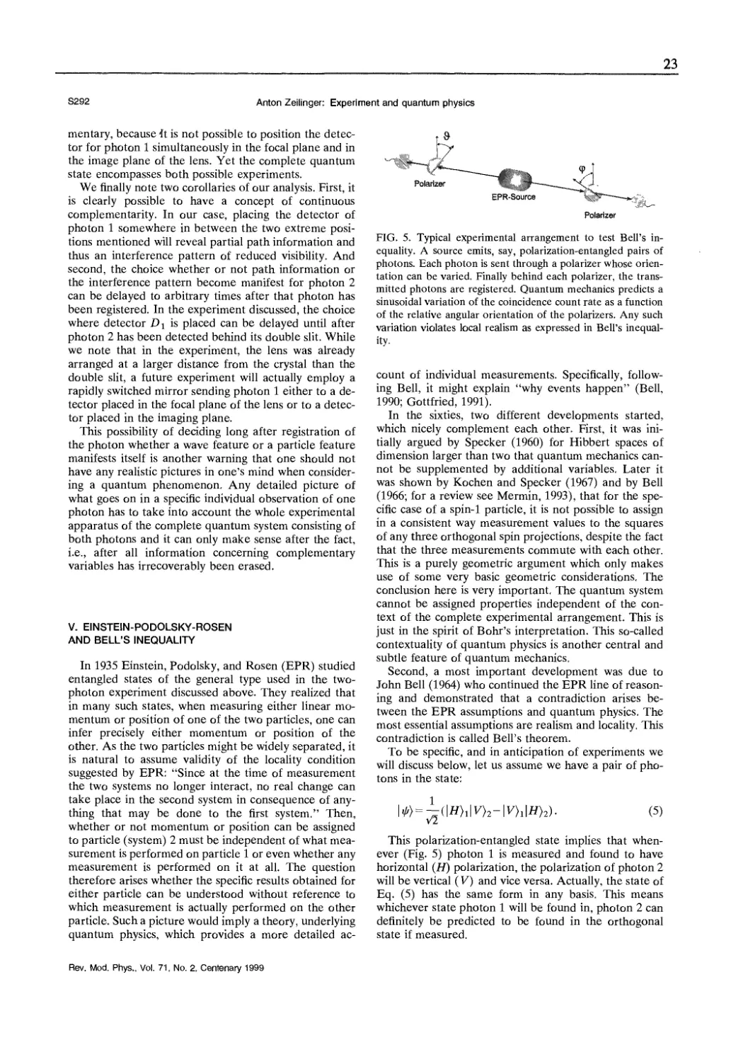
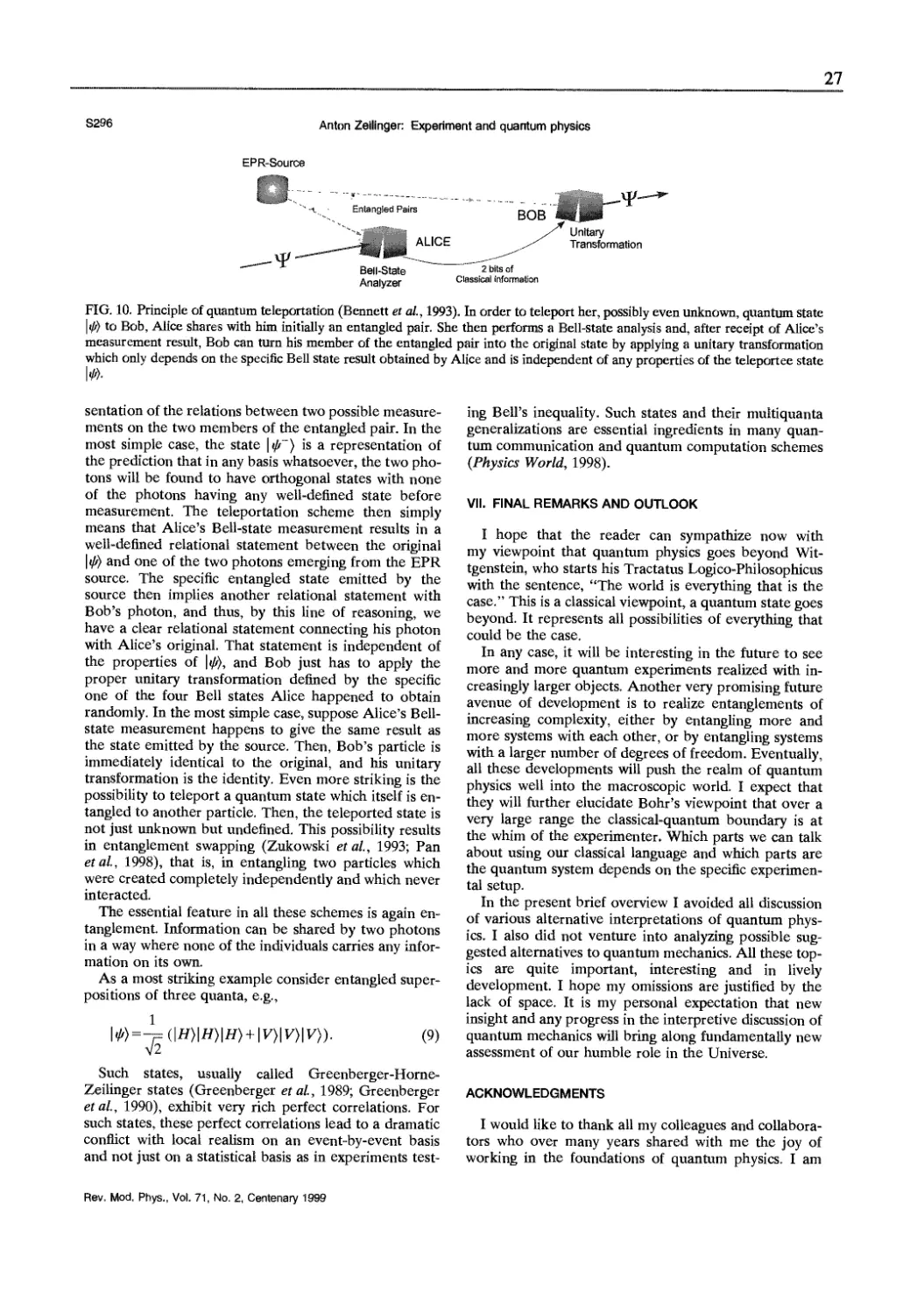
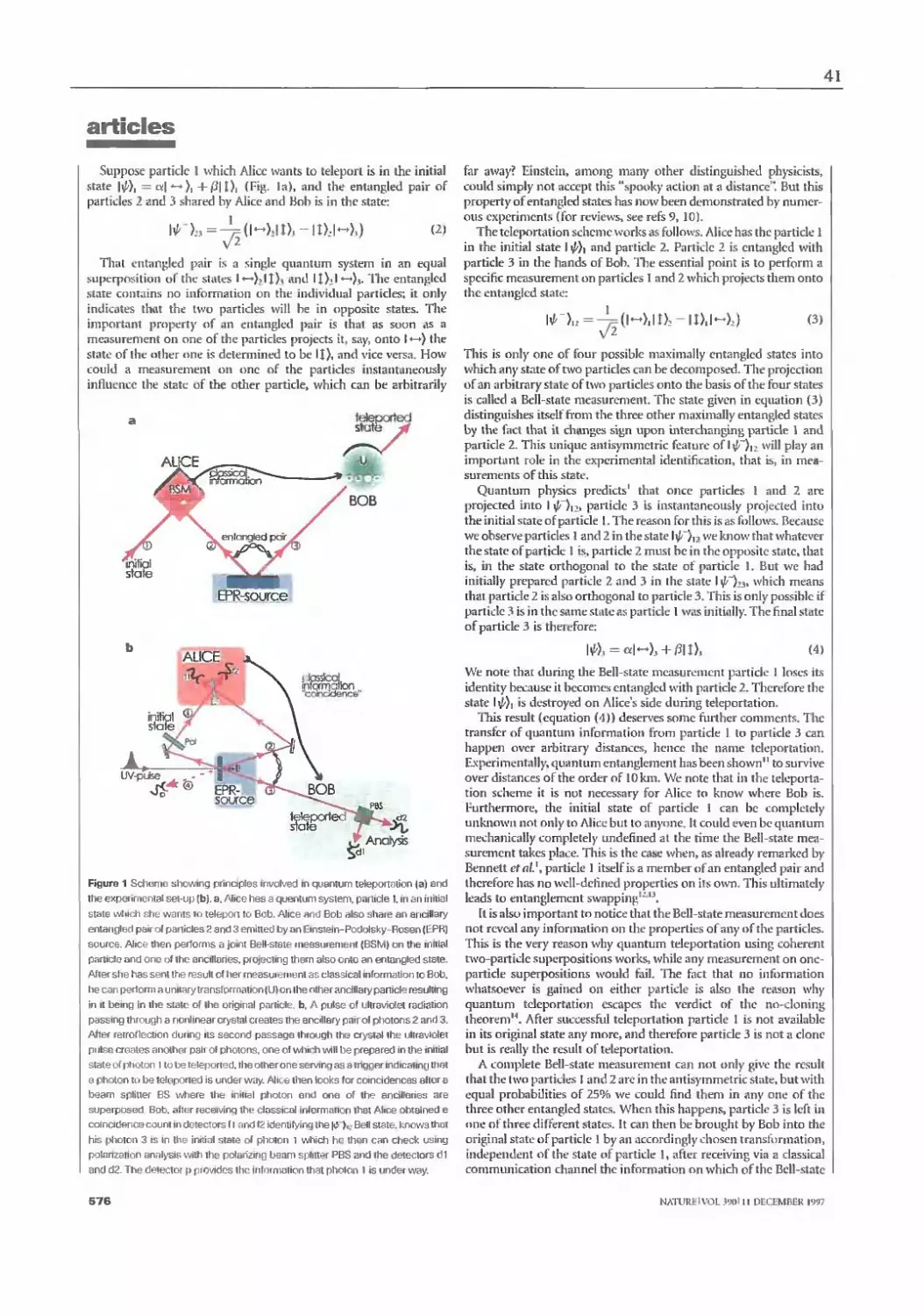
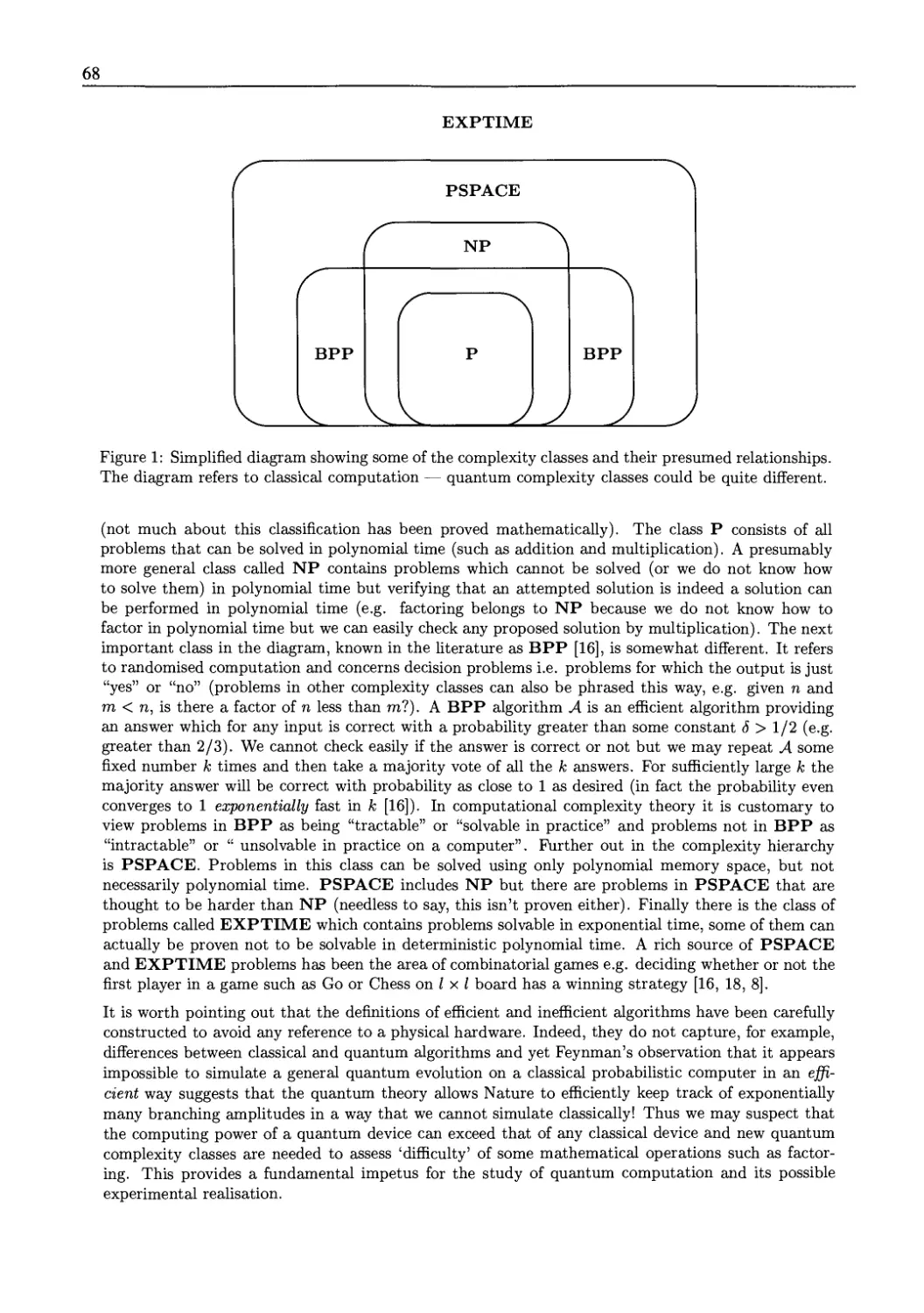
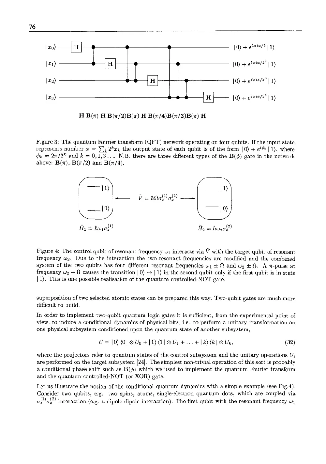
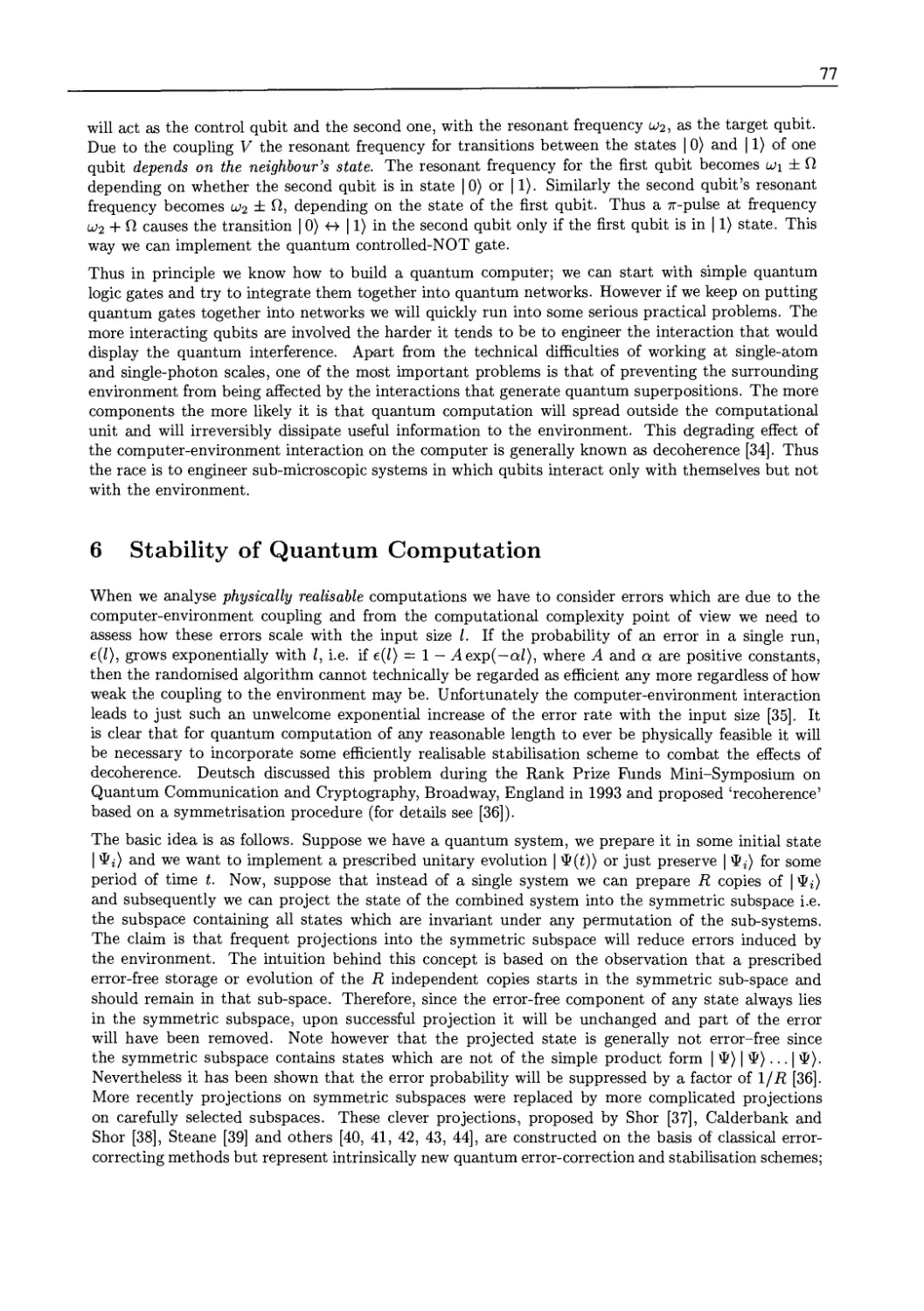
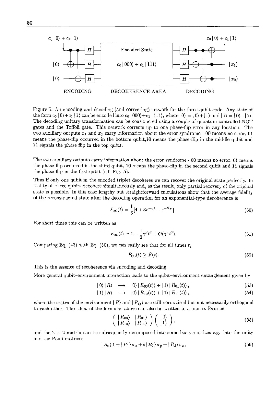
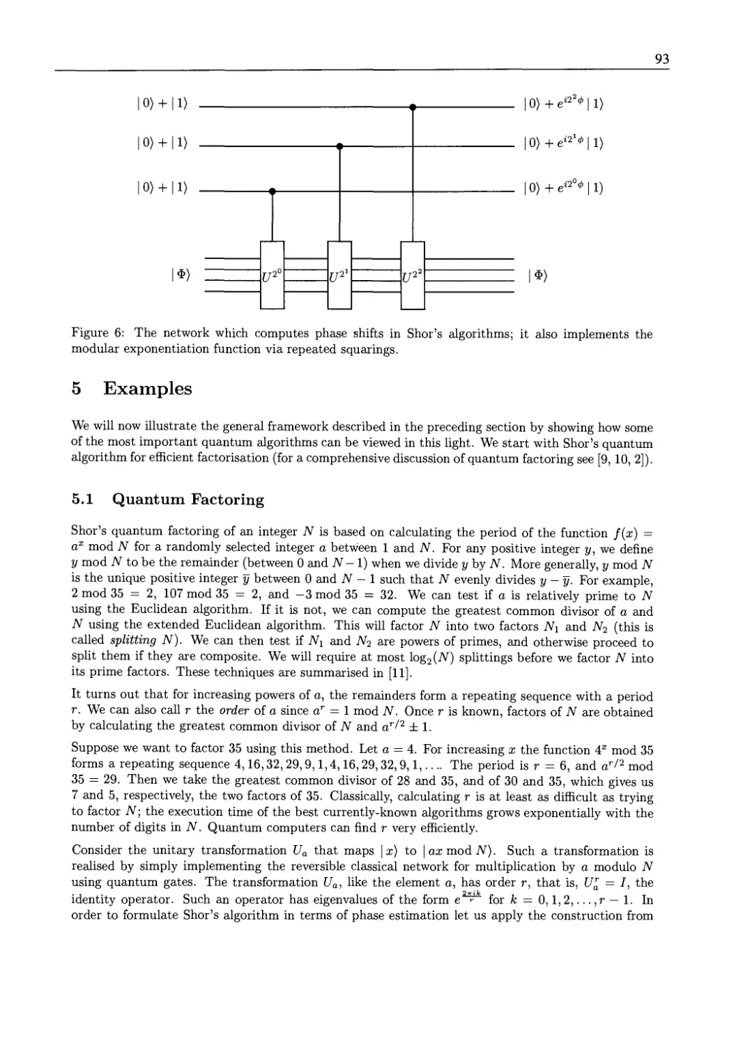
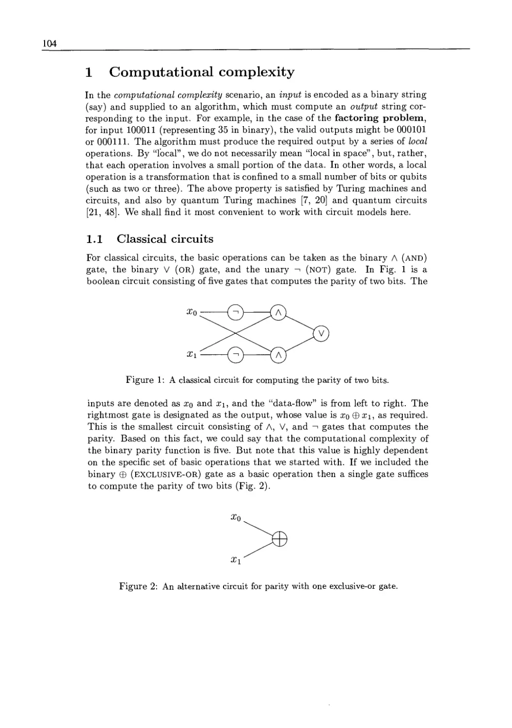
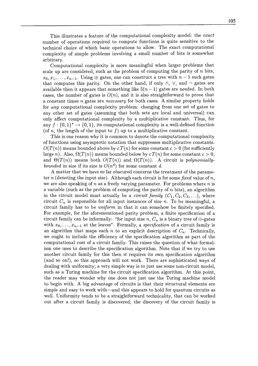
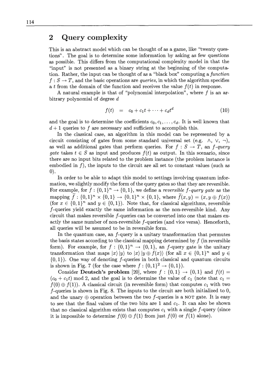
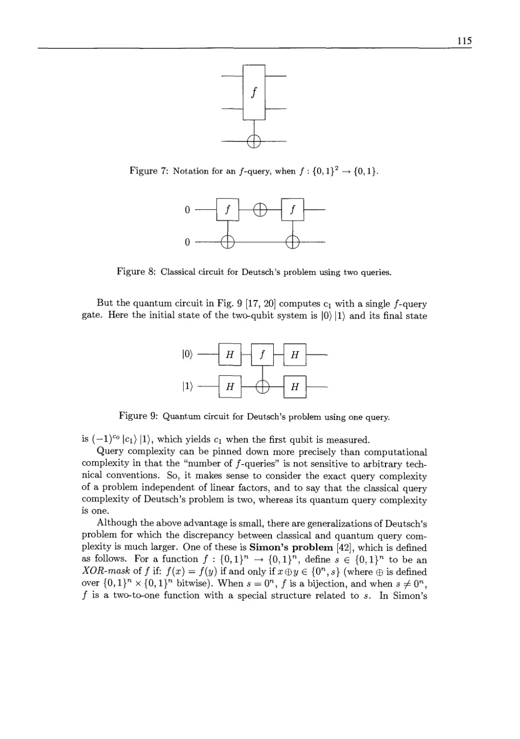
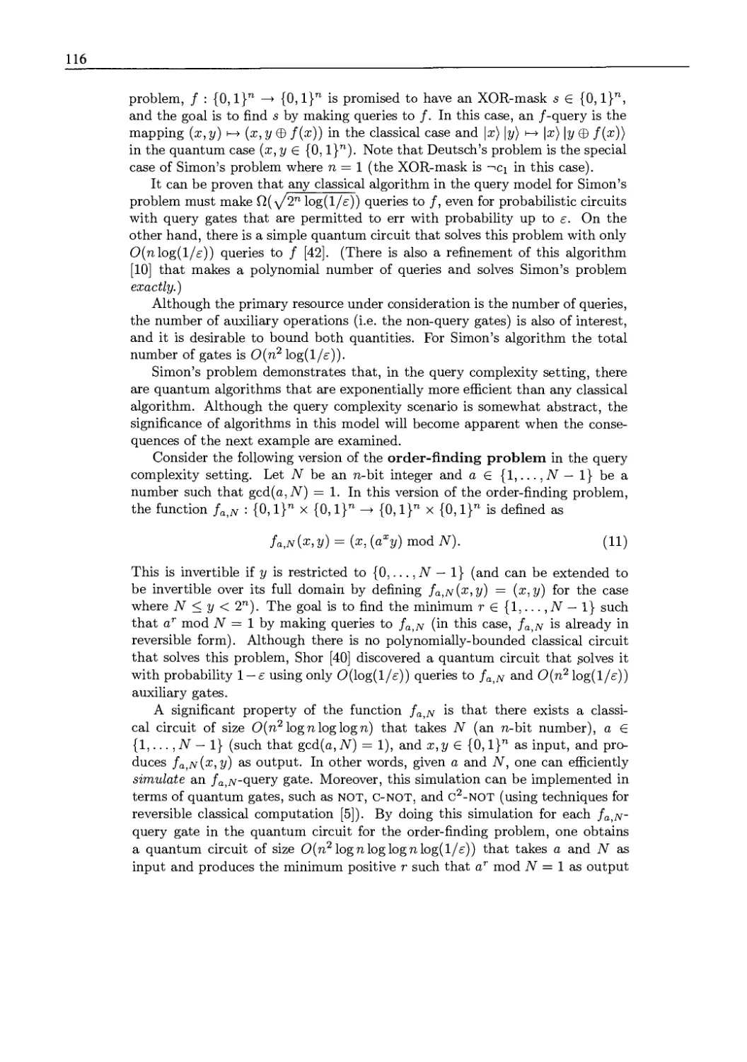
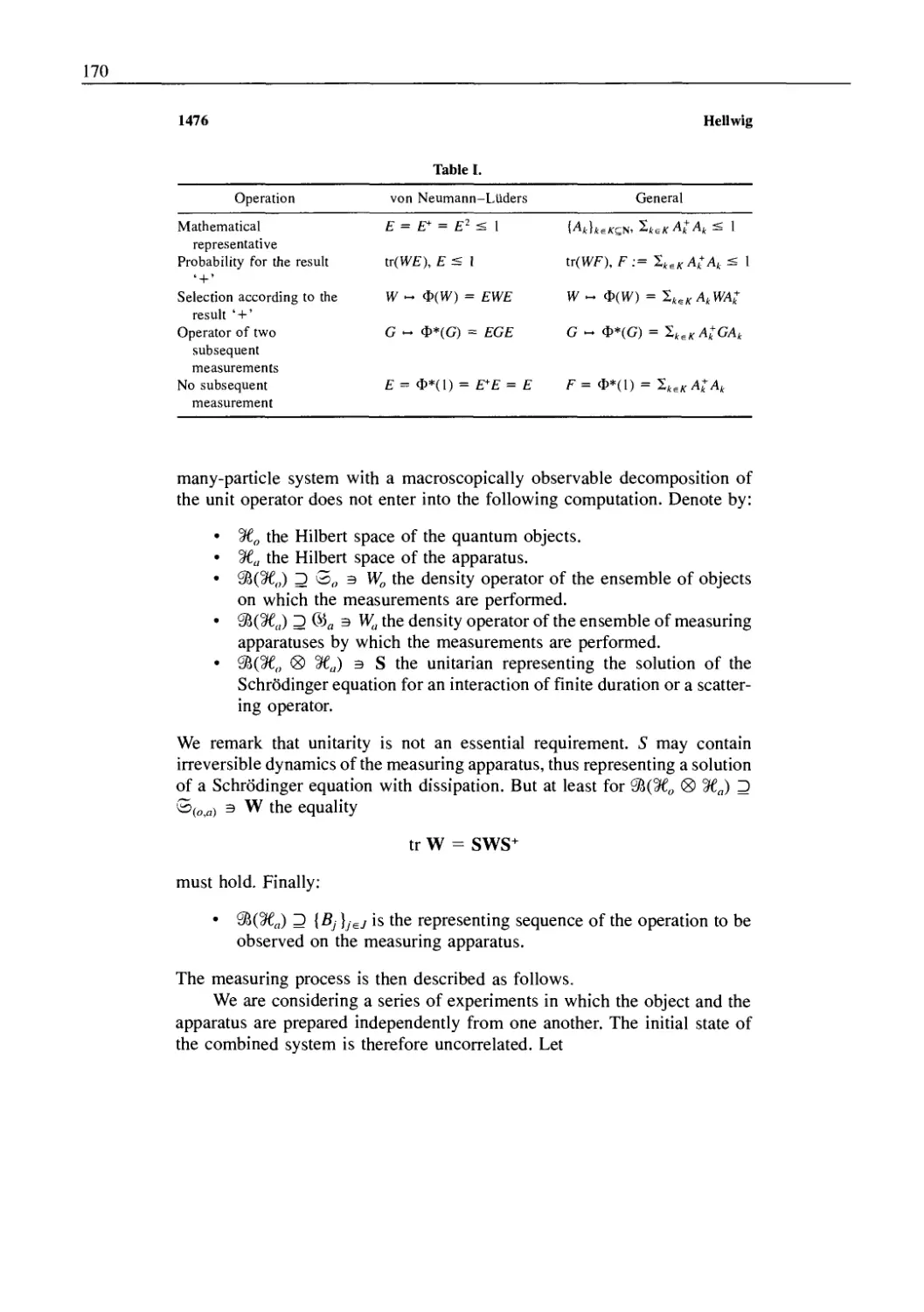
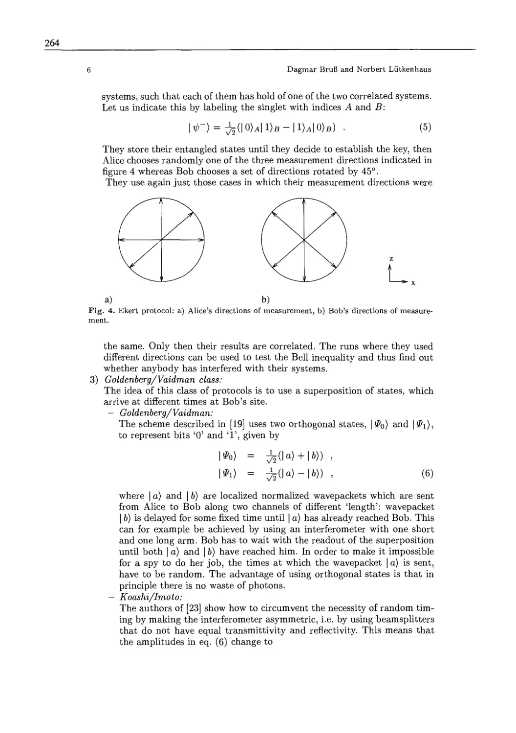
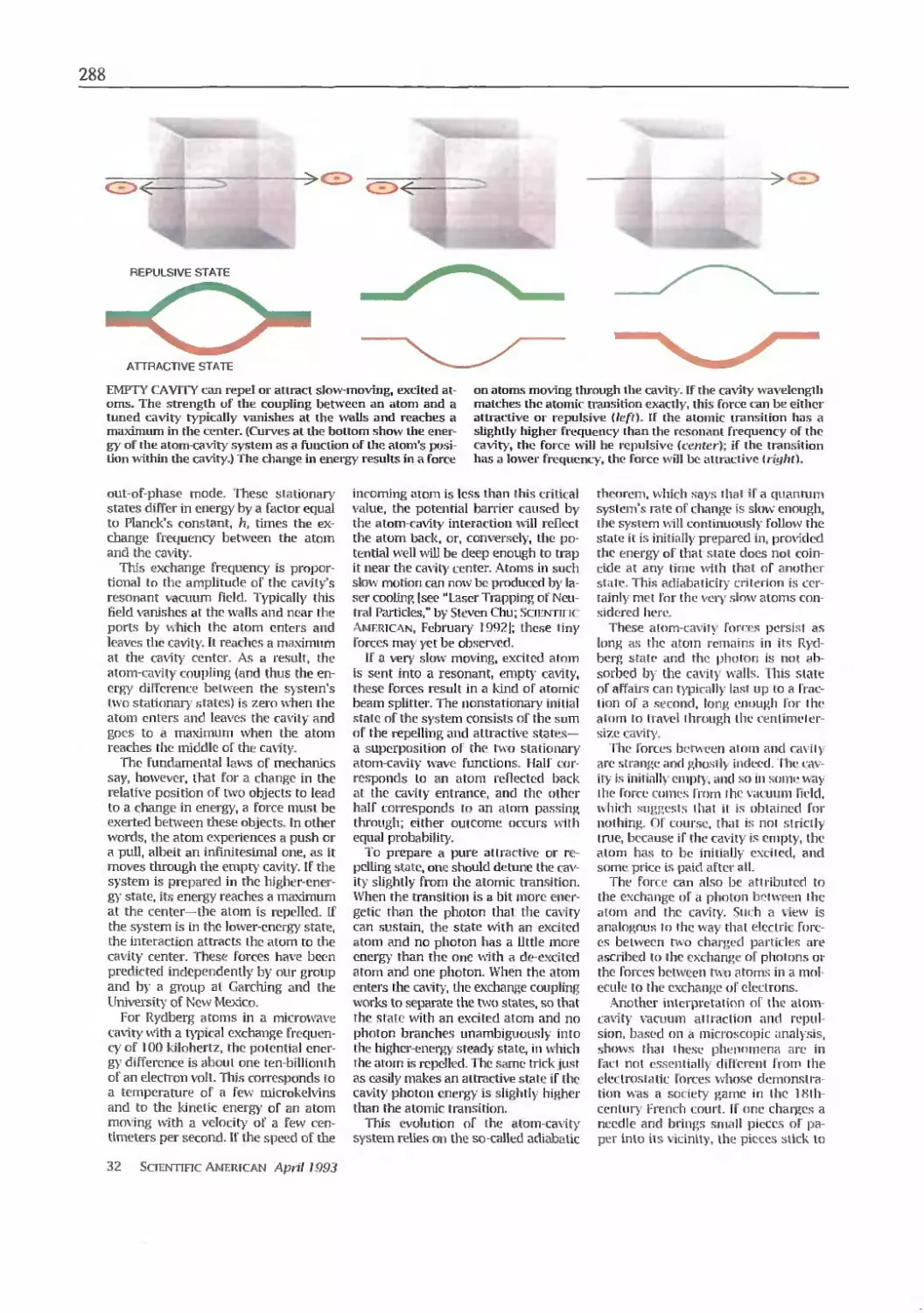
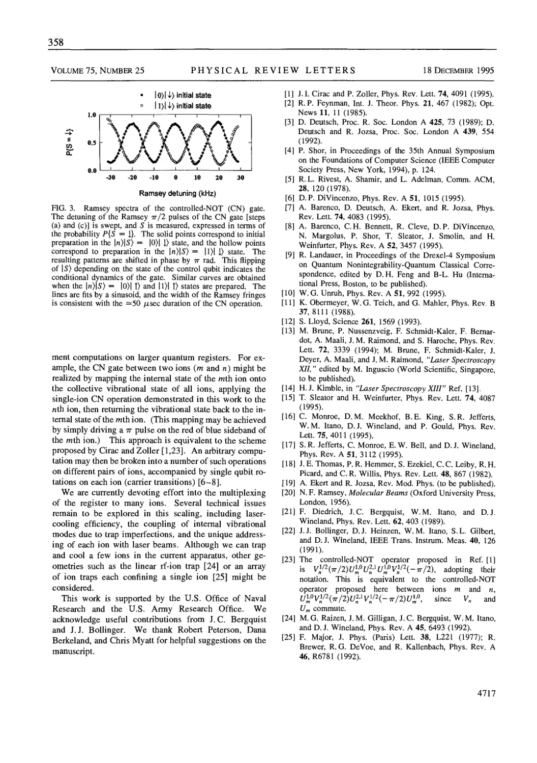
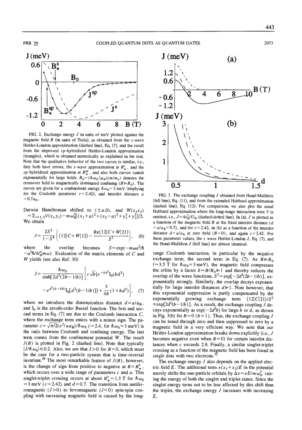
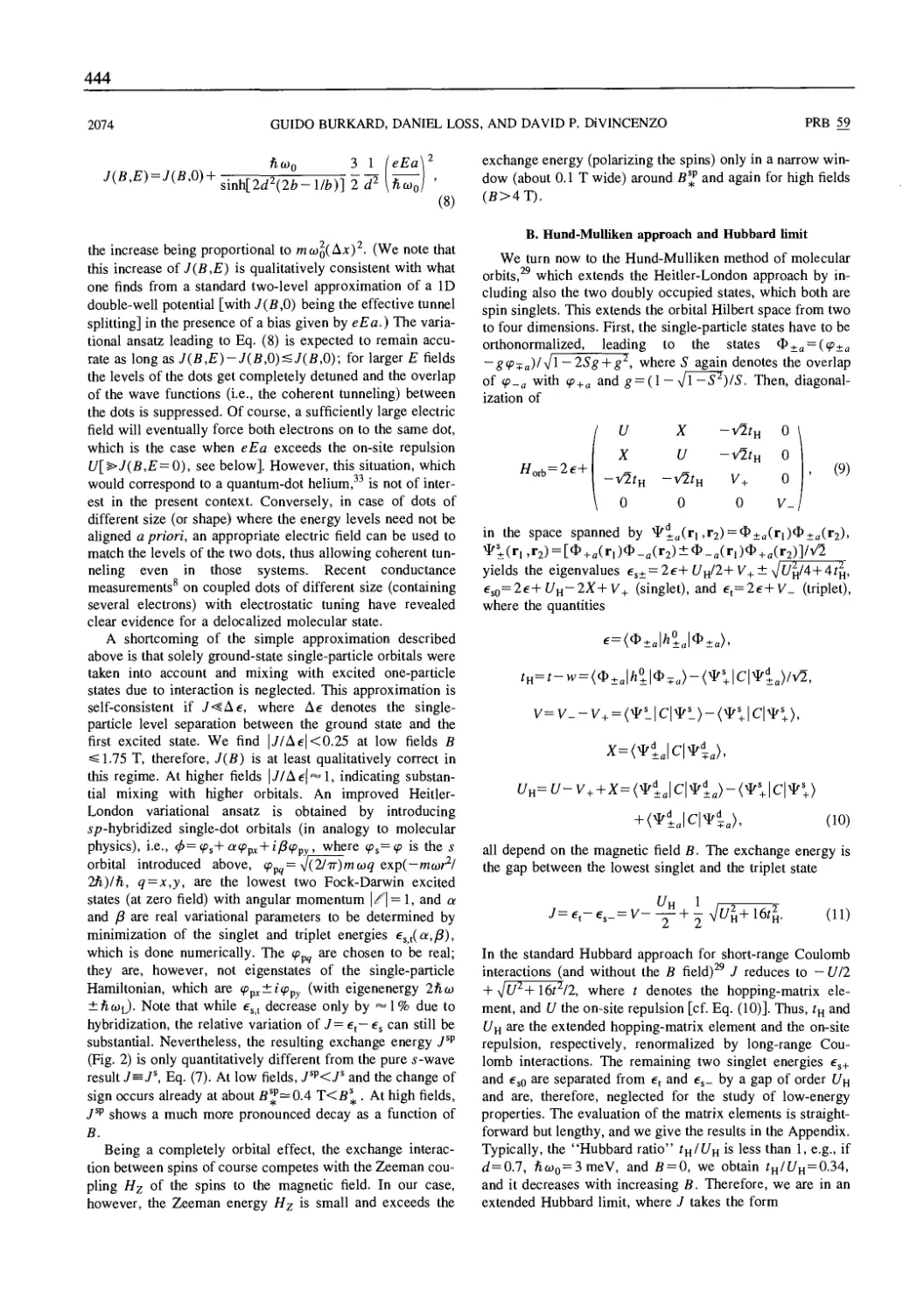
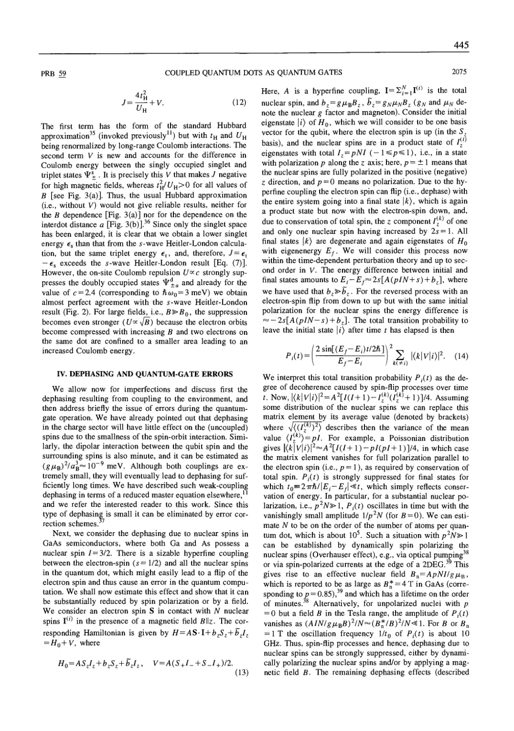
Текст
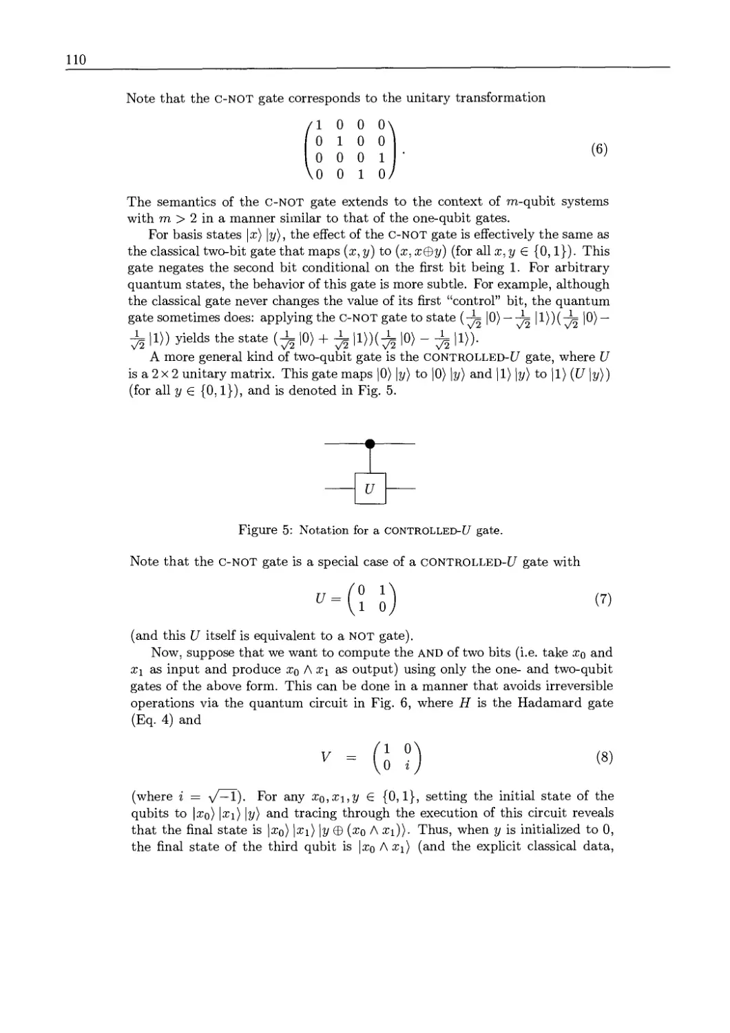
QUANTUM COMPUTATION
AND
QUANTUM INFORMATION
THEORY
QUANTUM COMPUTATION
AND
QUANTUM INFORMATION
THEORY
Reprint volume with introductory notes for
ISITMR Network School
12-23 July 1999 Villa Gualino, Torino, Italy
Editors
C. Macchiavello
University of Pavia, Italy
G. M. Palma
University Of Palermo, Italy
A. Zeilinger
University of Vienna, Austria
Yl^ World Scientific
WB SinaaDore • NewJersev • London •
Singapore • New Jersey • London • Hong Kong
Published by
World Scientific Publishing Co. Pte. Ltd.
P O Box 128, Fairer Road, Singapore 912805
USA office: Suite IB, 1060 Main Street, River Edge, NJ 07661
UK office: 51 Shelton Street, Covent Garden, London WC2H 9HE
British Library Cataloguing-in-Publication Data
A catalogue record for this book is available fronn the British Library.
The editors and the publisher would like to thank the authors and the following organizations for their assistance and their
permission to reproduce the articles found in this volume:
American Association for Advancement of Science
American Institute of Physics
American Physical Society
Elsevier Science Publishers
Institute of Physics Publishing
Kluwer Academic Publishers
National Academy of Sciences
Nature Publishing Group
Plenum Publishing Corporation
Royal Swedish Academy of Sciences
Scientific American
Springer Verlag
QUANTUM COMPUTATION AND QUANTUM INFORMATION THEORY
Copyright © 2000 by World Scientific Publishing Co. Pte. Ltd.
All rights reserved. This book, or parts thereof, may not be reproduced in any form or by any means, electronic
or mechanical, including photocopying, recording or any information storage and retrieval system now known
or to be invented, without written permission from the Publisher.
For photocopying of material in this volume, please pay a copying fee through the Copyright Clearance Center,
Inc., 222 Rosewood Drive, Danvers, MA 01923, USA. In this case permission to photocopy is not required from
the publisher.
ISBN 981-02-4117-8
Printed in Singapore.
Preface
What can you do when you write and read your information on single atoms? How
secret are your messages if you conceal them in the state of a single photon? Can you
teleport at a distant point the unknown state of a particle? These questions, which would
have seemed idle - if not meaningless - just a decade ago have now become hot topic of
research. Quantum Information Theory has indeed revolutionised our view of what is the
nature of information, imposing itself as a new paradigm. Since the early seminal papers in
the 80' s the rate at which results have appeared in the scientific literature, mirroring the
rapid progresses in this - now mature - discipline, has been astonishing. As the field still
lacks of a comprehensive textbook it is a hard job for the newcomer to find his way in the
existing literature. The job being made harder by the very interdisciplinary nature of this
new area of research, with deep roots both in the foundations of Quantum Mechanics as
well as of Information Theory and Computer Science. In this volume we have asked some
of the leading researchers in the field to select and annotate a choice of articles in their
area in order to give the reader a broad perspective of the present stage of research in all
the various aspects of quantum information processing. The articles have been chosen with
particular attention to their tutorial value. Each expert has been the curator of one section
of the book. This initiative has been taken as part of the summer school on "Quantum
Computation and Quantum Information Theory" organised by the Institute for Scientific
Interchange Foundation in Villa Gualino, Torino, July '99.
In our choice of topics we have tried to give a broad overview of both the theoretical
foundation of the field as well as of its practical design and experimental aspects.
The opening chapter is dedicated to the physical ingredients of the theory, introducing
key concepts like entanglement and non locality which are the core of the quantum world,
followed by a chapter dealing with the experimental aspects of entanglement measurement
and manipulation. Quantum world manifests itself with a puzzling weird looking behavior
which confuses our classical perception of daily world. Indeed it is this "weirdness" which,
when properly harnessed, allows for new efficient forms of information coding, transmission
and manipulation.
Three sections are then devoted to clarifying the computer - science aspects of the theory.
The first of these chapters is an overview of quantum algorithms. The aim is to clarify which
features of quantum theory make possible an exponential gain of resource in computation
and to provide a unified description of the known quantum algorithms. This is followed
by a chapter specially written for this book devoted to the theory of quantum complexity,
in which the complexity classes of quantum algorithms are analysed with respect to the
resources needed to implement them. The discussion of this part of the book ends with a
VI
chapter dedicated to quantum error correction. The extention of the powerful techniques
developed for the reliable transmission and storage of classical information are far from
being straightforwardly transferable in the quantum domain. Quantum error correction is
an example of area of research in which, in the time span of less than two years the theory
has reached a high level of sophistication, starting basically from sctatch.
The three following chapters overview three different aspects of information
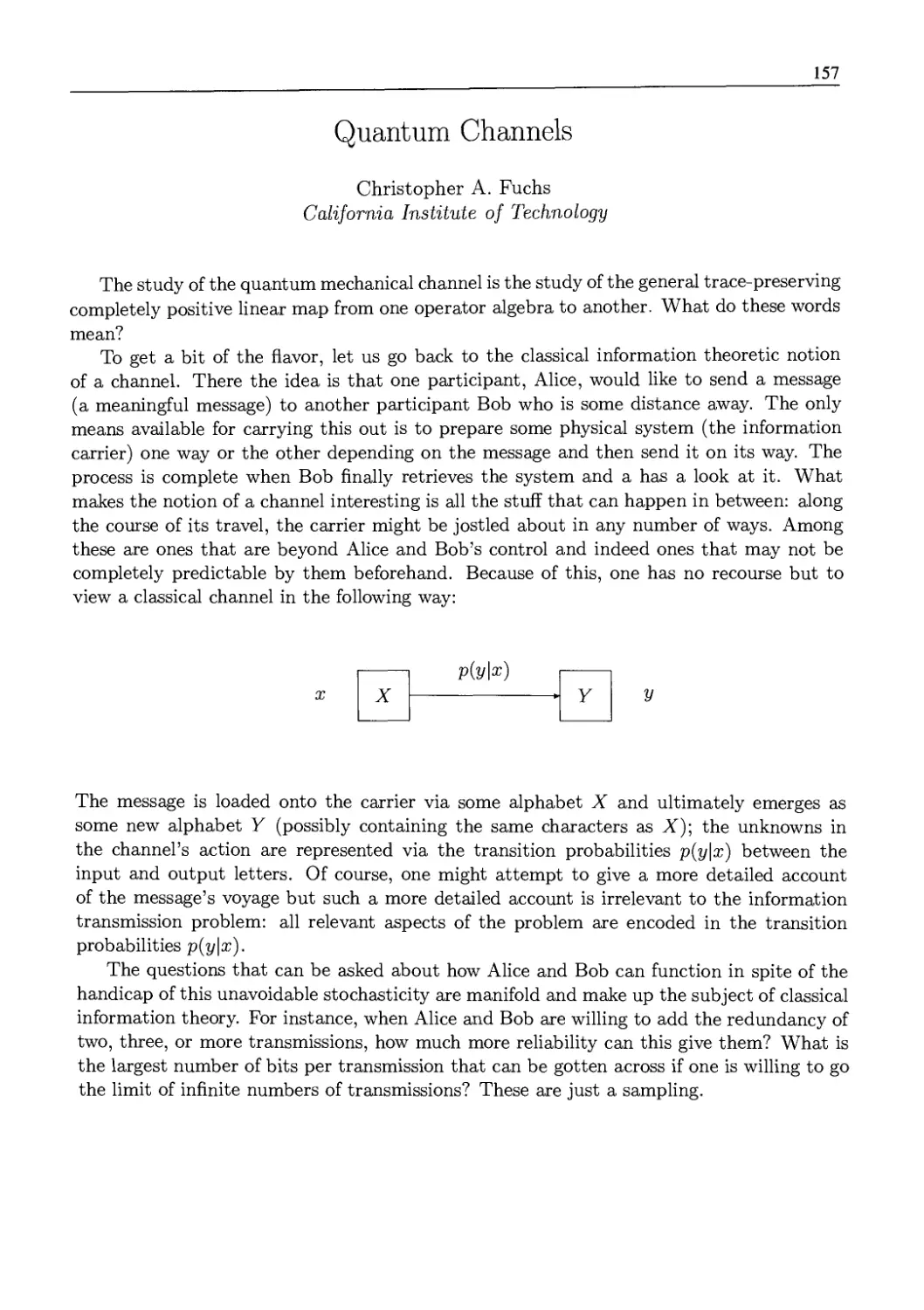
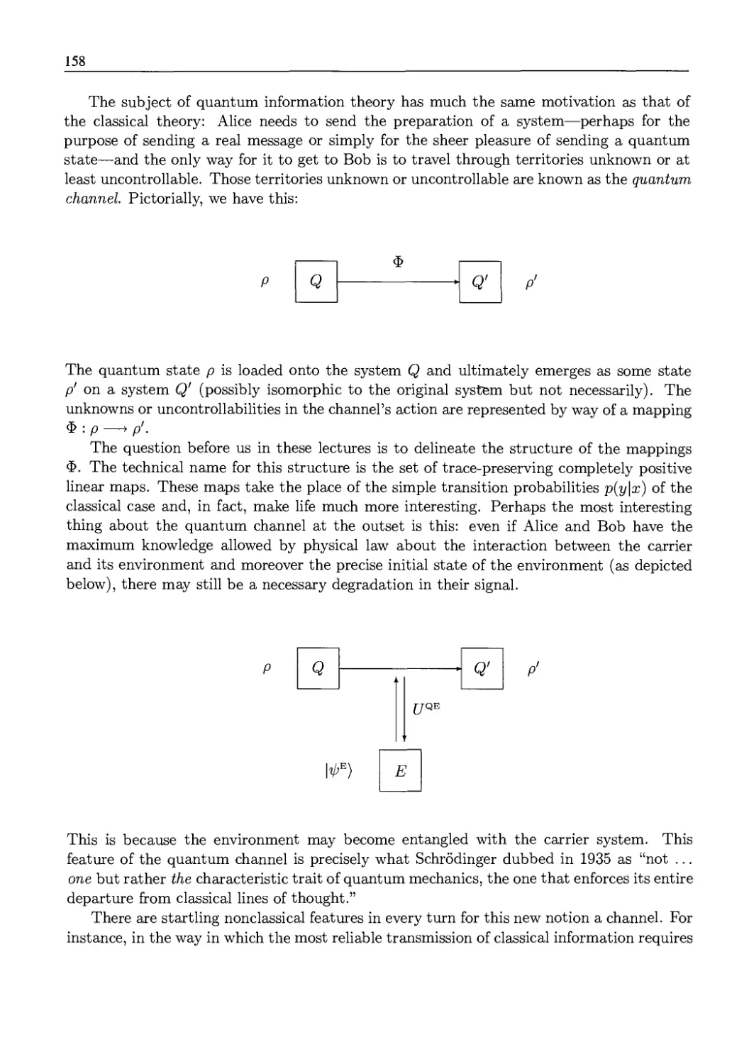
transmission. The Quantum Channels section provides an introduction to the tools used to describe
noisy quantum channels and to measure the amount of reliable information sent through
them via appropriate encoding and decoding. Related to this is the section on Long distance
Quantum Communication, which describes protocols aiming at achieving the transmission
of coherent quantum information over long distances overcoming the effects of the external
environment. This is followed by a section devoted Quantum Cryptography, the art of
sharing secret keys with the help of quantum mechanics. One of the oldest branch of quantum
information theory, it is now in the realm of technological applications, with existing pre
industrial prototypes. The related chapter gives an overview of both the theoretical and
the experimental aspects of the subject.
The remaining part of the book reviews all the candidate technologies for the practical
implementation of quantum computing devices. These can be broadly divided into two
categories: atomic systems (like cavity Q.E.D., cold trapped ions) and mesoscopic ones (like
Josephson junctions, quantum dots), with some technologies at the borderline between the
two, as NMR and cold atoms in optical lattices. While atomic systems are characterised by
a relatively easily controllable dynamics their scalability remains an open problem. On the
other hand mesoscopic systems, although vulnerable to the spoiling action of the
environment, open the possibility of large scale integration.
At the end of the book a bibliography is appended, with all the papers reproduced or
quoted in the introduction plus a few others chosen directly by the editors. We have made
no attempt neither to be comprehensive of all contributions to the field nor to be exhaustive
of all the research going on in Quantum Information Theory. We apologise to whoever feels
neglected in this list.
The limited space at our disposal has left no room for a description of many other recent
developments of the theory, like the thermodynamics of entanglement, quantum cloning,
topological quantum computation, just to mention some. As these topics are at the front
line of such a rapidly expanding field it would have been extremely difficult to make a choice
of papers which could be considered as reference. This, we feel, will be probably possible
in the next few years.
Our thanks go to all the lecturers to the summer school on "Quantum Computation
and Quantum Information Theory" organised by the Institute for Scientific Interchange
Foundation, Villa Gualino, Torino, which have patiently helped us in selecting the papers
of each section and which have written the relative introductory notes.
C. Macchiavello
CM. Palma
A. Zeilinger
Vll
CONTENTS
Preface
1
3
Introductory Concepts
1. Introductory Concepts
A. Zeilinger (University of Vienna)
1.1 D. M. Greenberger, M. A. Home and A. Zeilinger
Multiparticle Interferometry and the Superposition Principle
Physics Today 46, No. 8, 22-29 (August 93) 4
1.2 A. Zeilinger
Quantum Entanglement: A Fundamental Concept Finding its Applications
Physica Scripta, T76, 203-209 (1998) 12
1.3 A. Zeilinger
Experiment and the Foundations of Quantum Physics
Rev. Mod. Phys. 71(2), S288-S297 (1999) 19
Quantum Entanglement Manipulation 29
2. Quantum Entanglement Manipulation 31
D. Bouwmeester (Center of Quantum Computation, University of Oxford)
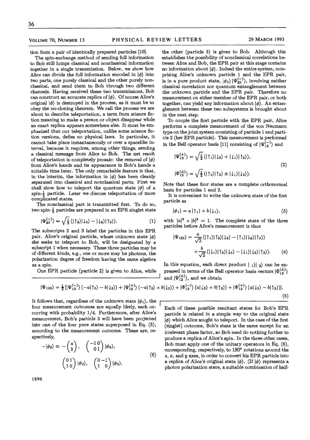
2.1 C. H. Bennett, G. Brassard, C. Crepeau, R. Jozsa, A. Peres and
W. K. Wootters,
Teleporting an Unknown Quantum State via Dual Classic and
Einstein-Podolsky-Rosen Channels
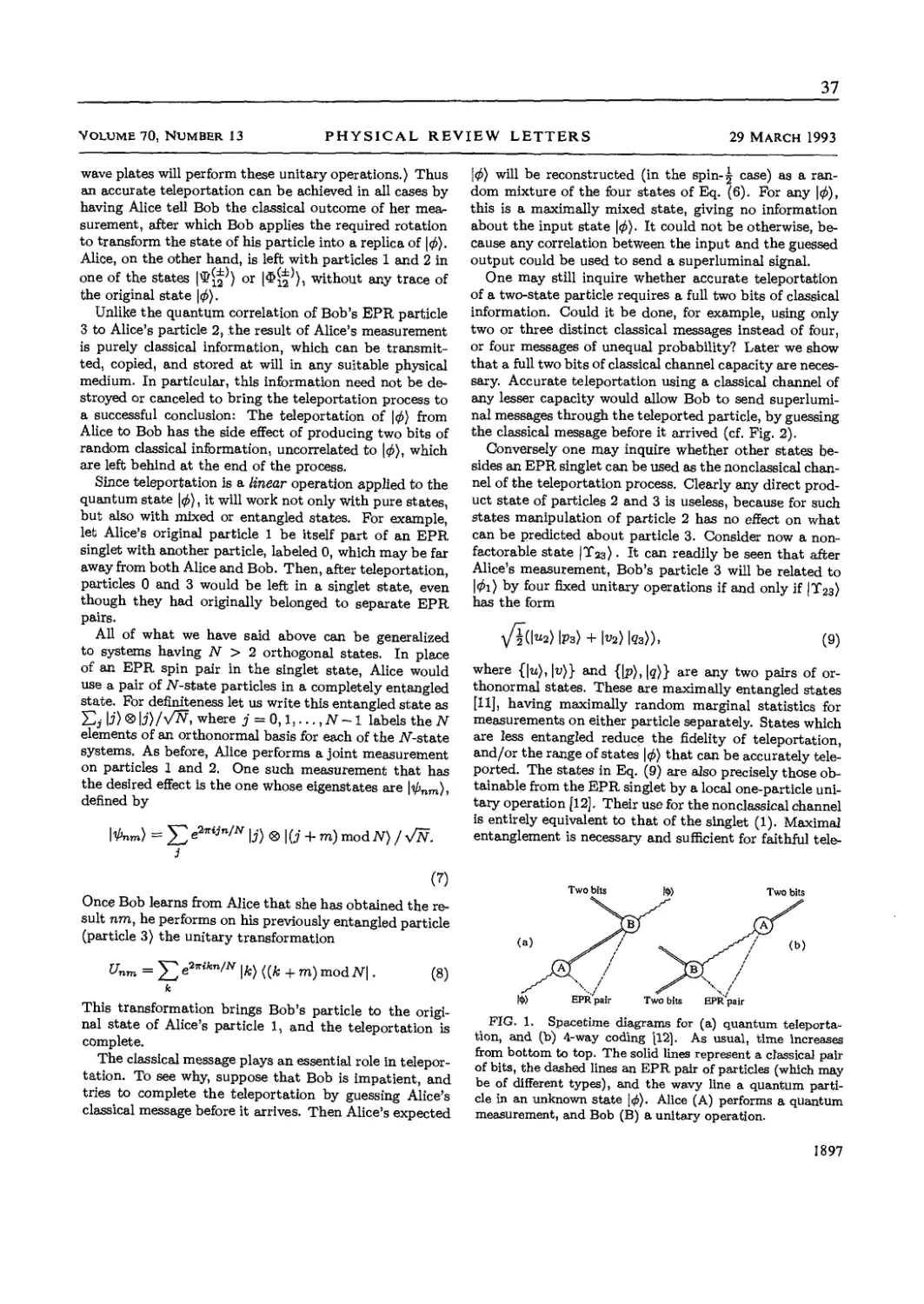
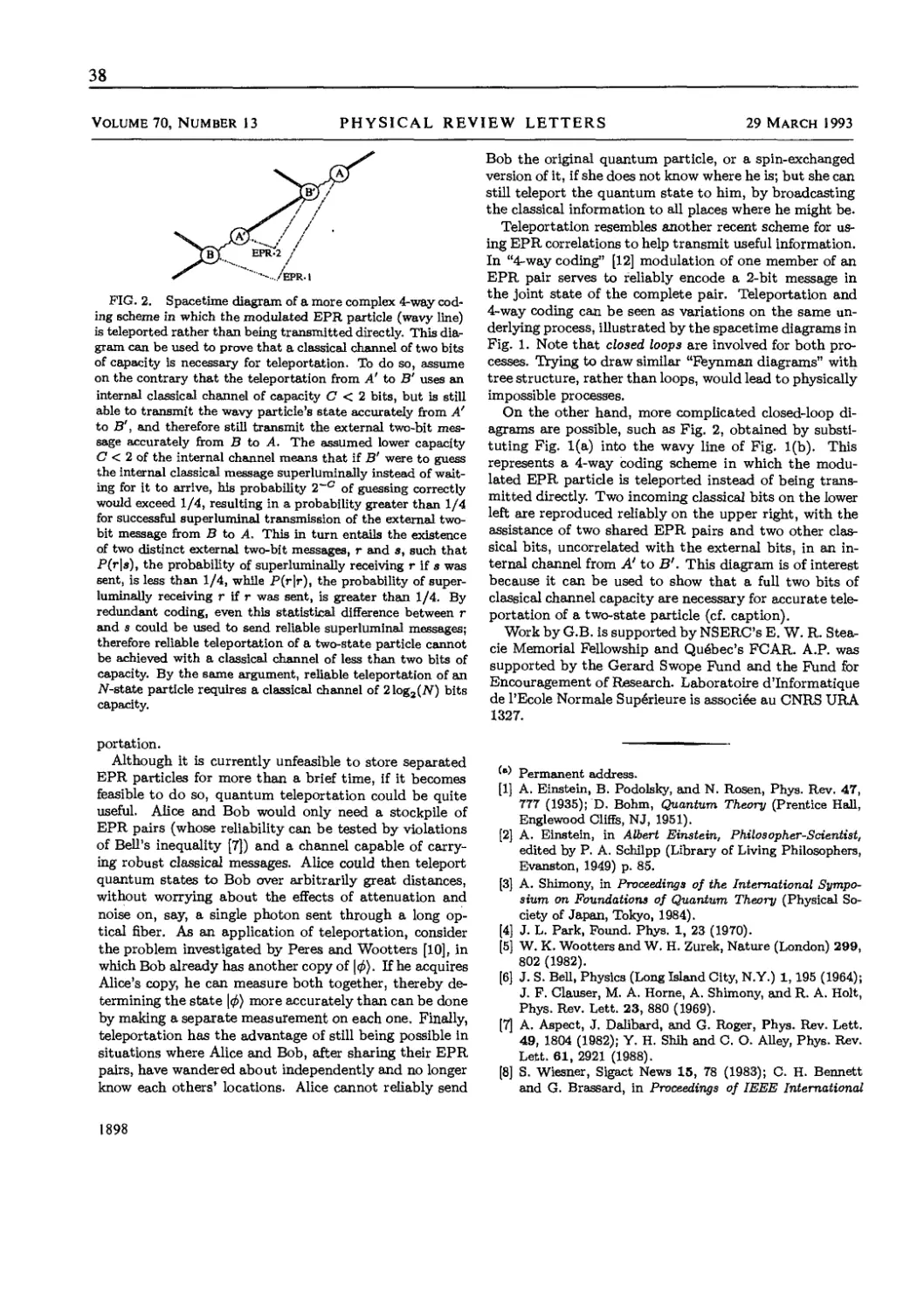
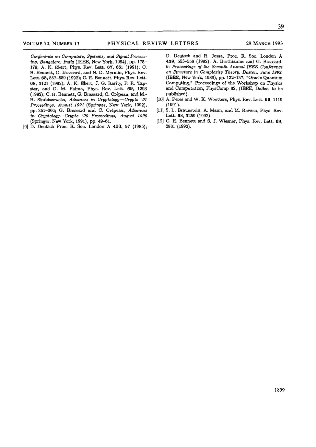
Phys. Rev, Lett. 70(13), 1895-1899 (1993) 35
2.2 D. Bouwmeester, J.-W. Pan, K. Mattle, M. Eibl, H. Weinfurter and
A. Zeilinger
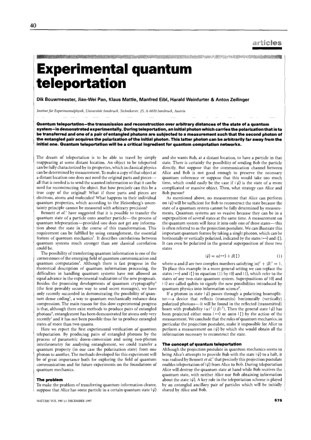
Experimental Quantum Teleportation
Nature 390, 575-579 (1997) 40
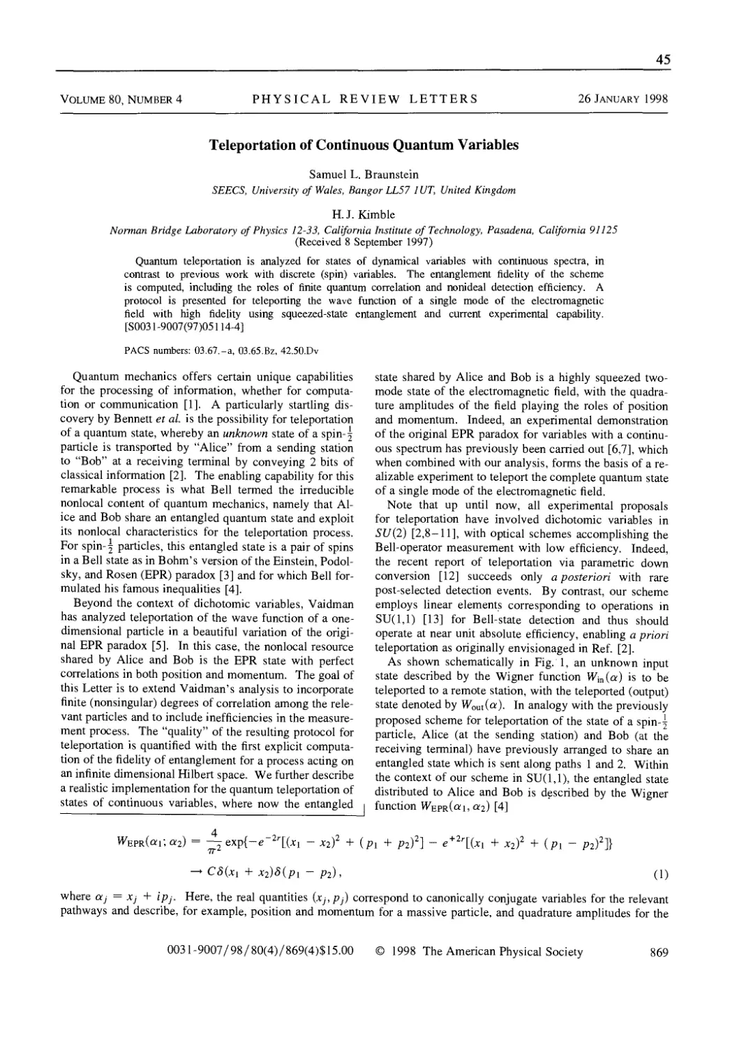
2.3 S. L. Braimstein and H. J. Kimble
Teleportation of Continuous Quantum Variables
Phys. Rev. Lett. 80(4), 869-972 (1998) 45
2.4 D. M. Greenberger, M. A. Home and A. Zeilinger
Going Beyond BelVs Theorem,
in BelVs Theorem, Quantum Theory and Conception df the Universe
M. Kafatos (Ed.) (Kluwer, Dodrecht, 1989) 49
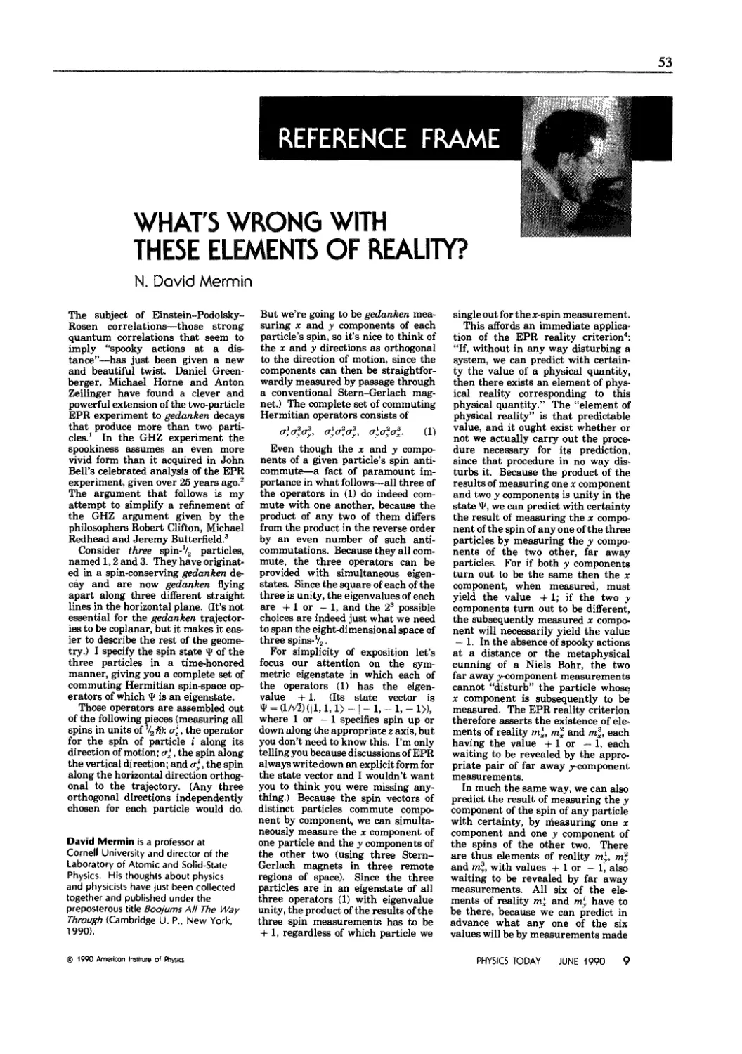
2.5 N. David Mermin
What is Wrong with These Elements of Reality
Physics Today, 43, No. 6, 9 & 11 (June 1990) 53
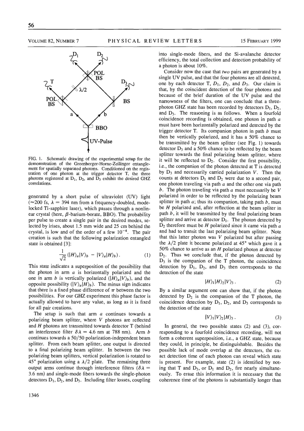
2.6 D. Bouwmeester, J.-W. Pan, M. Daniell, H. Weinfurter and A, Zeilinger
Observation of Three-Photon Greenberger-Home-Zeilinger Entanglement
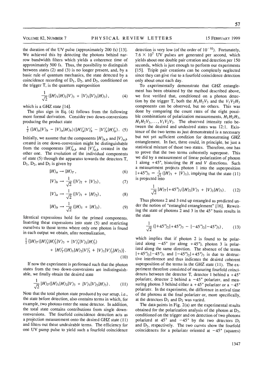
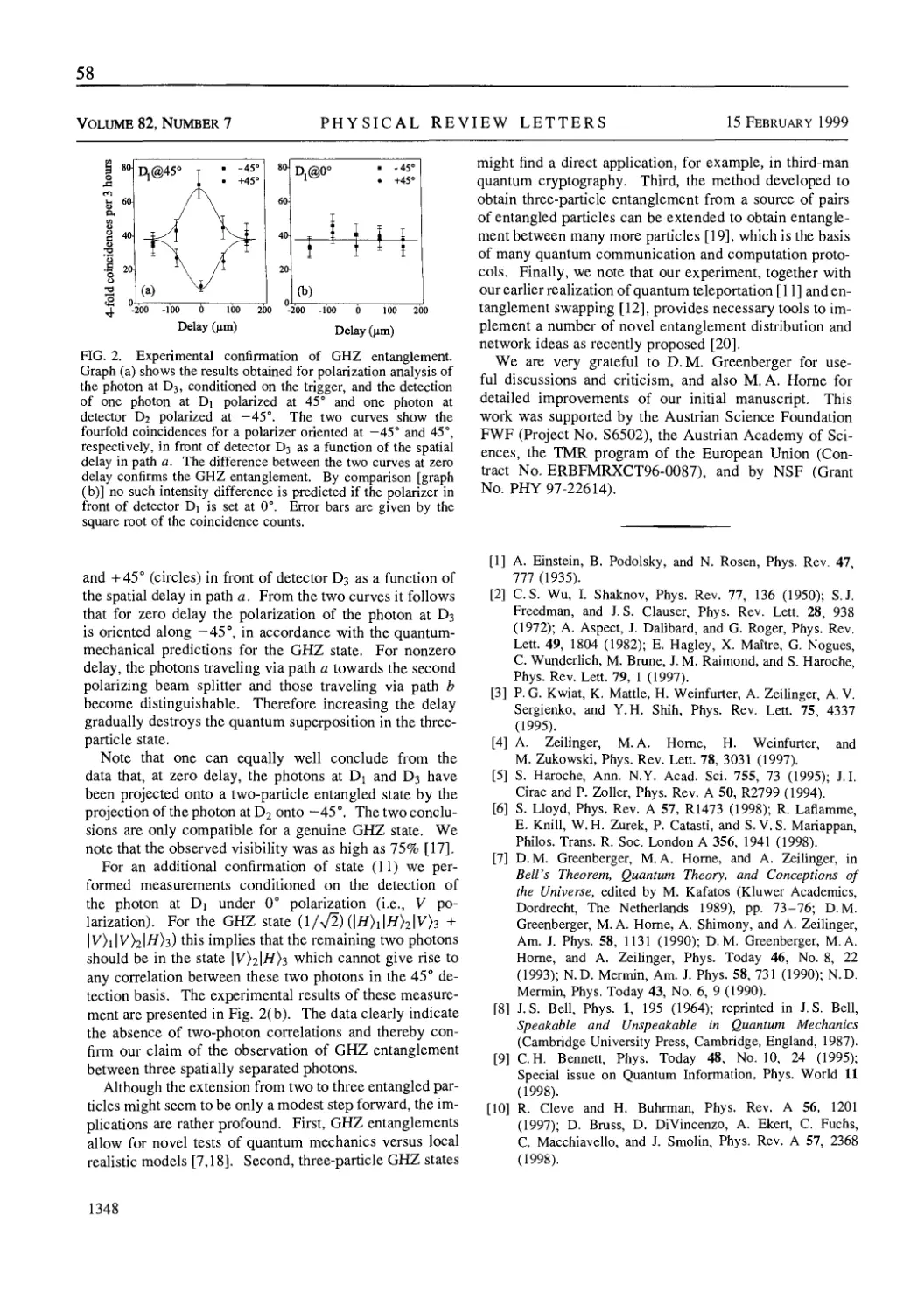
Phys. Rev. Lett. 82(7), 1345-1349 (1999) 55
Vlll
Quantum Algorithms 61
3. Quantum Algorithms 63
A. Ekert (Center for Quantum Computation, University of Oxford)
3.1 A. Ekert and C. Macchiavello
An Overview of Quantum Computing
in Unconventional Models of Computation, 19-44, C. S. Calude, J. Casti
and M. J. Dinneen Eds., Springer Series in Discrete Mathematics
and Theoretical Computer Science (Springer, Singapore, 1998) 66
3.2 R. Cleve, A. Ekert, L. Henderson, C. Macchiavello and M. Mosca
On Quantum Algorithms
Complexity 4(1), 33-42 (Sept/Oct 1998) also preprint quant-ph/9903061 86
Quantum Complexity 101
4. An Introduction to Quantum Complexity Theory
R. Cleve (University of Calgary) 103
Quantum Error Correction 129
5. Quantum Error Correction 131
D. DiVincenzo (IBM Research Laboratories)
5.1 P. W. Shor
Scheme for Reducing Decoherence in Quantum, Computer Mem,ory
Phys. Rev. A 52(4), R2493-R2496 (1995) 134
5.2 A. M. Steane
Error Correcting Codes in Quantum, Theory
Phys. Rev. Lett. 77(5), 793-797 (1996) 138
5.3 D. Gottesman
Class of Quantum Error-Correcting Codes Saturating the Quantum,
Hamming Bound
Phys. Rev. A 54(3), 1862-1868 (1996) 143
5.4 D. P. DiVincenzo and P. W. Shor
Fault-Tolerant Error Correction with Efficient Quantum Codes
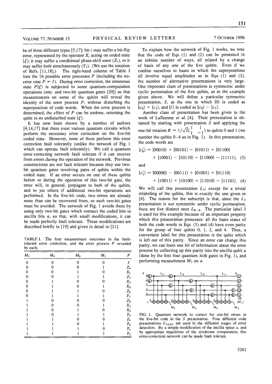
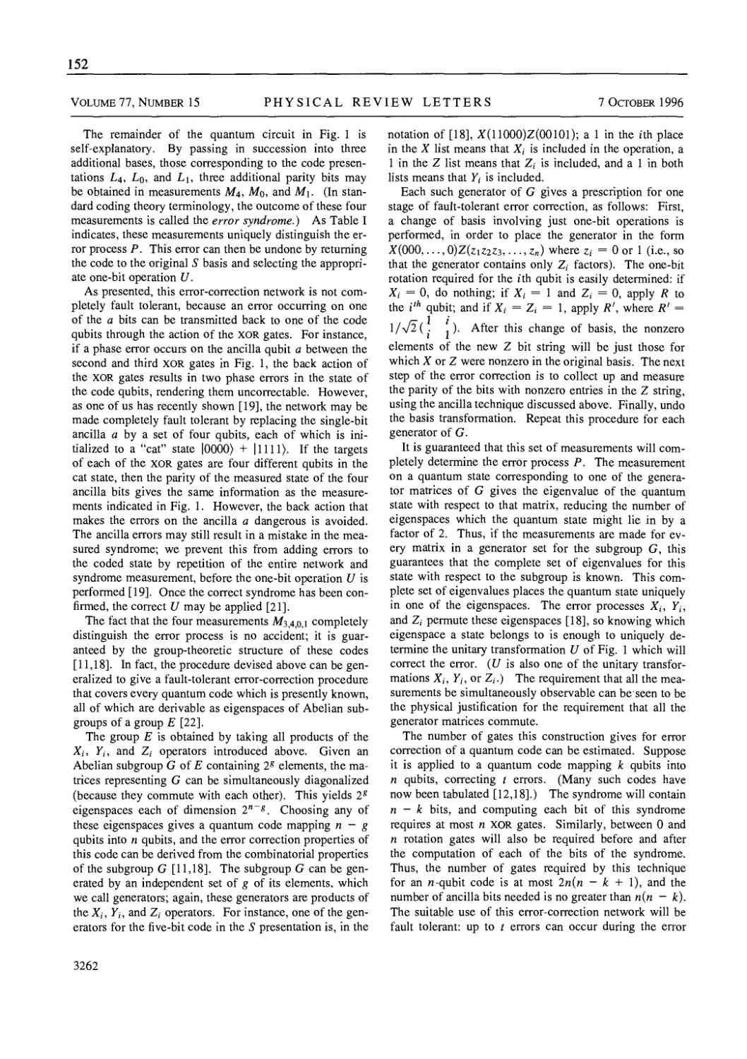
Phys. Rev. Lett. 77(15), 3260-3263 (1996) 150
Quantum Channels 155
6. Quantum Channels 157
C. A. Puchs (Cahfornia Institute of Technology)
6.1 K,-E. Hellwig
General Scheme of Measurement Processes
Int. J. Theor. Phys. 34(8), 1467-1479 (1995) 161
6.2 M.-D. Choi
Completely Positive Linear Maps on Complex Matrices
Lin. Alg. Appl. 10, 285-289 (1975) 174
IX
6.3 B. Schumacher
Sending Entanglement Through Noisy Quantum Channels
Phys. Rev. A 54(4), 2614-2628 (1996) 180
6.4 H. Barnum, C. M. Caves, C. A. Puchs, R. Jozsa and B. Schumacher
Noncommuting Mixed States Cannot Be Broadcast
Phys. Rev. Lett. 76(15), 2818-2821 (1996) 195
6.5 B. Schimiacher and M. D. Westmoreland
Sending Classical Information via Noisy Quantum, Channels
Phys. Rev. A 56(1), 131-138 (1997) 199
6.6 C. A. Puchs
Nonorthogonal Quantum States Maximize Classical Inform,ation Capacity
Phys. Rev. Lett. 79(6), 1163-1166 (1997) 207
Entanglement Purification and Long-Distance Quantum
Communication
211
7. Long-Distance Quantum Communication 213
H. Briegel (Ludwig-Maximilians-Universitaet, Munich)
7.1 H.-J. Briegel, W. Diir, J. L Cirac and P. Zoller
Quantum, Repeaters: The Role of Imperfect Local Operations in
Quantum, Communication
Phys. Rev. Lett. 81(26), 5932-5935 (1998) 217
7.2 C. H. Bennett, G. Brassard, S. Popescu, B. Schimiacher, J. A. Smolin
and W. K. Wootters
Purification of Noisy Entanglement and Faithful Teleportation
via Noisy Channels
Phys. Rev. Lett. 76(5), 722-725 (1996) 221
7.3 D. Deutsch, A. Ekert, R. Jozsa, C. Macchiavello, S. Popescu and A. Sanpera
Quantum Privacy Amplification and the Security of Quantum Cryptography
over Noisy Channels
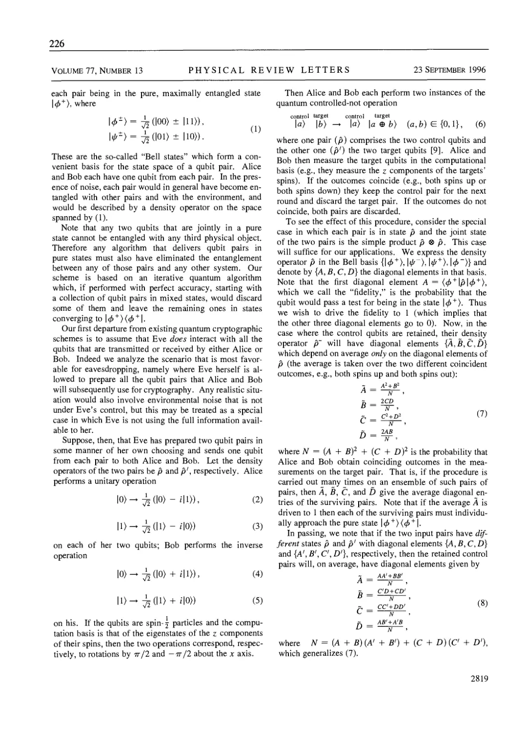
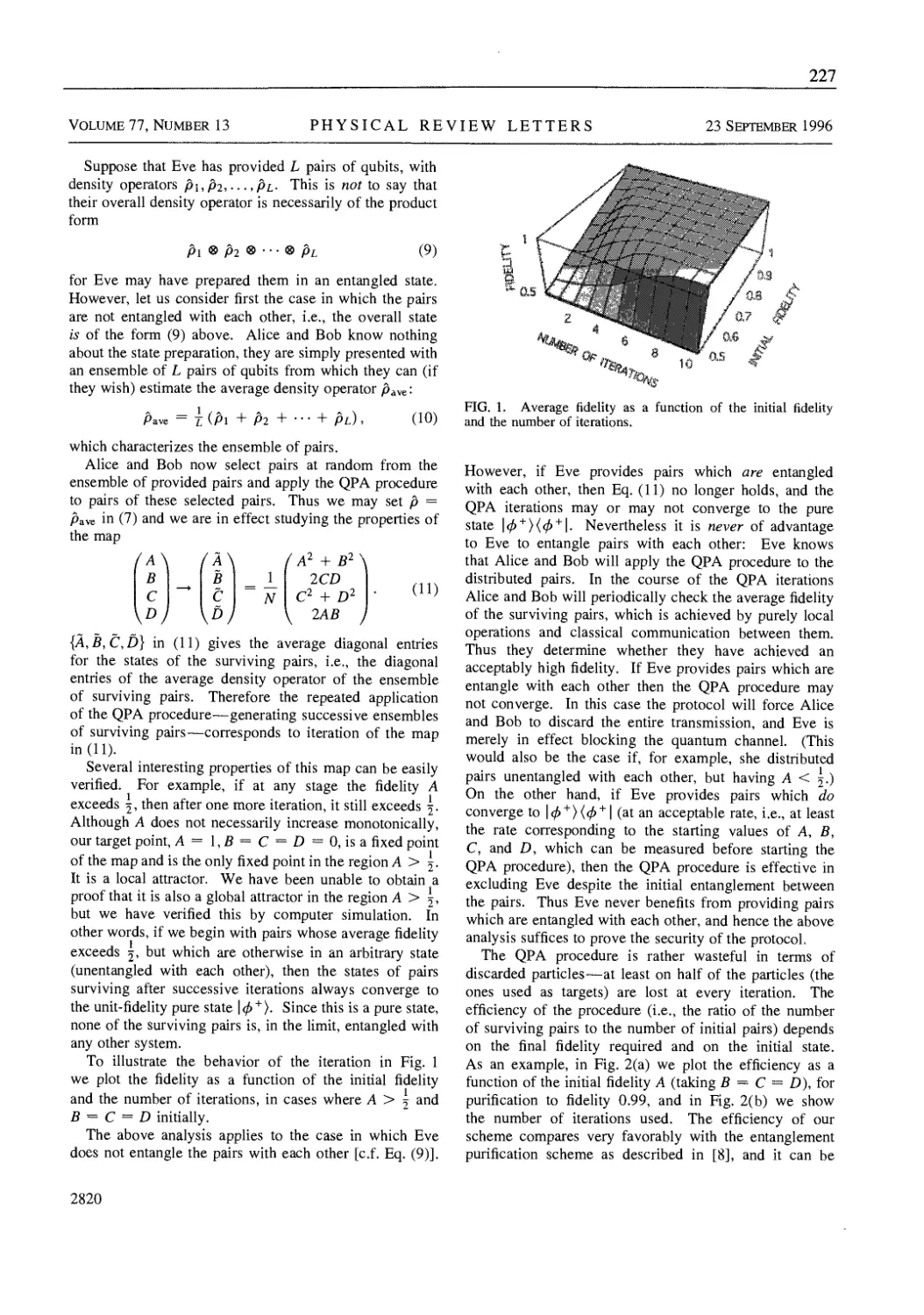
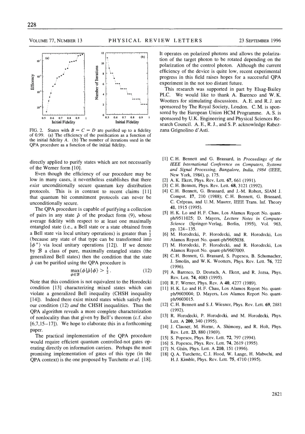
Phys. Rev. Lett. 77(13), 2818-2821 (1996) 225
7.4 S. J. van Enk, J. L Cirac and P. Zoller
Photonic Channels for Quantum Communication
Science 279, 205-208 (1998) 229
Quantum Key Distribution 233
8. Quantum Key Distribution 235
G. Ribordy, N. Gisin and H. Zbinden (University of Geneva)
8.1 W. Tittel, G. Ribordy and N. Gisin
Quantum, Cryptography
Physics World, pp. 41-45 (March 1998) 240
8.2 H. Zbinden, N. Gisin, B. Huttner, A. Muller and W. Tittel
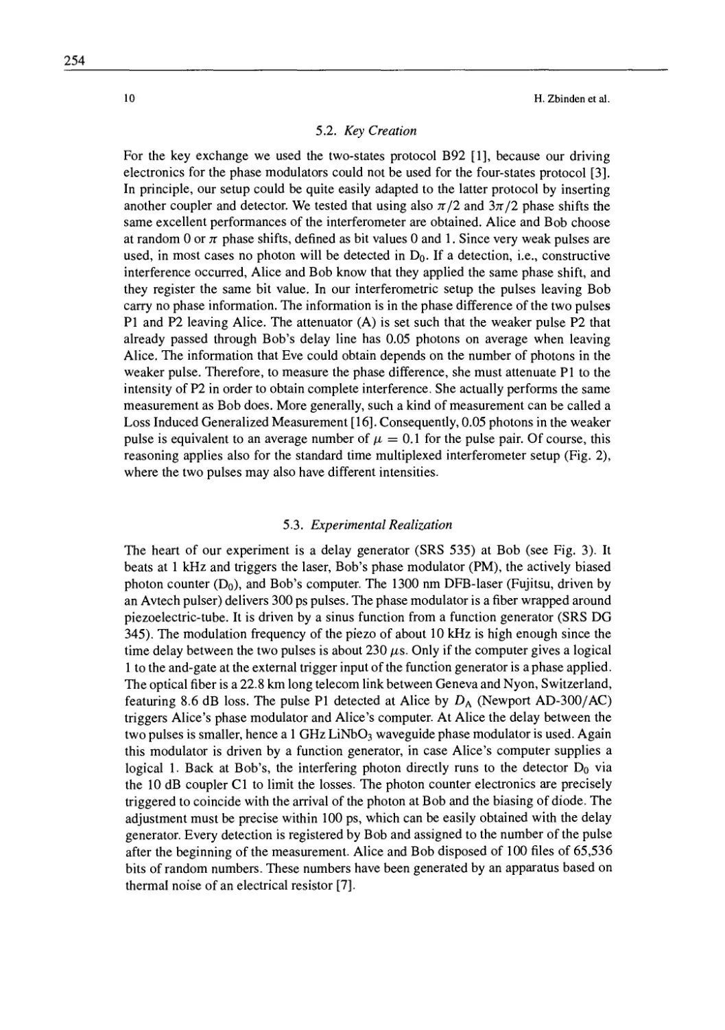
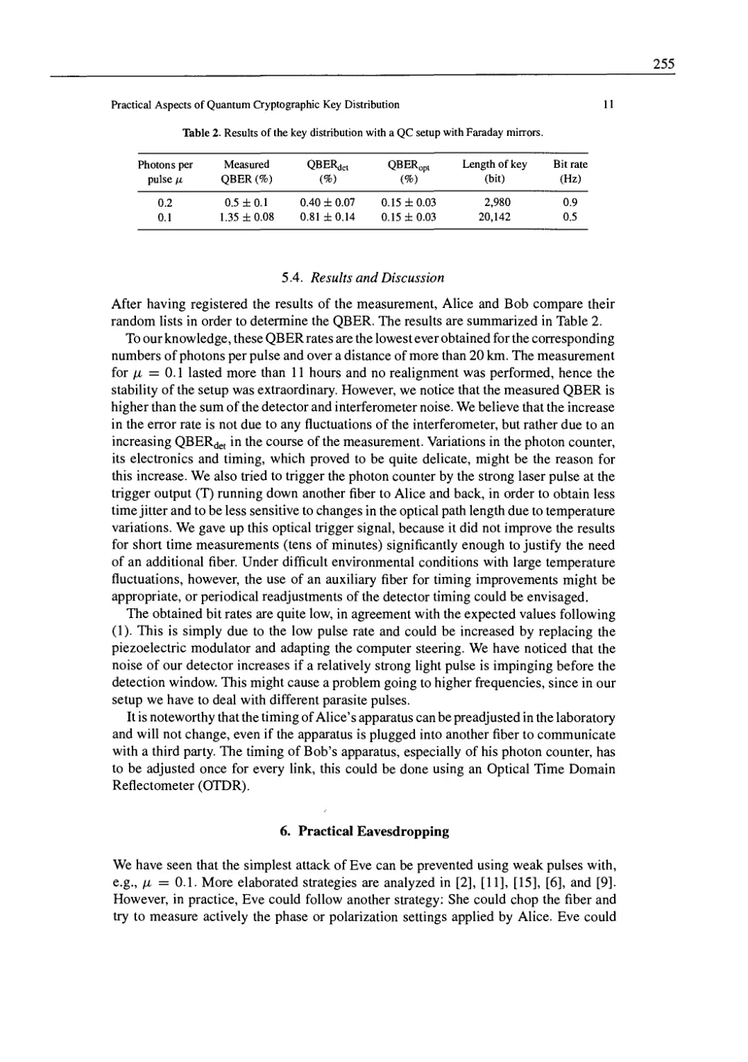
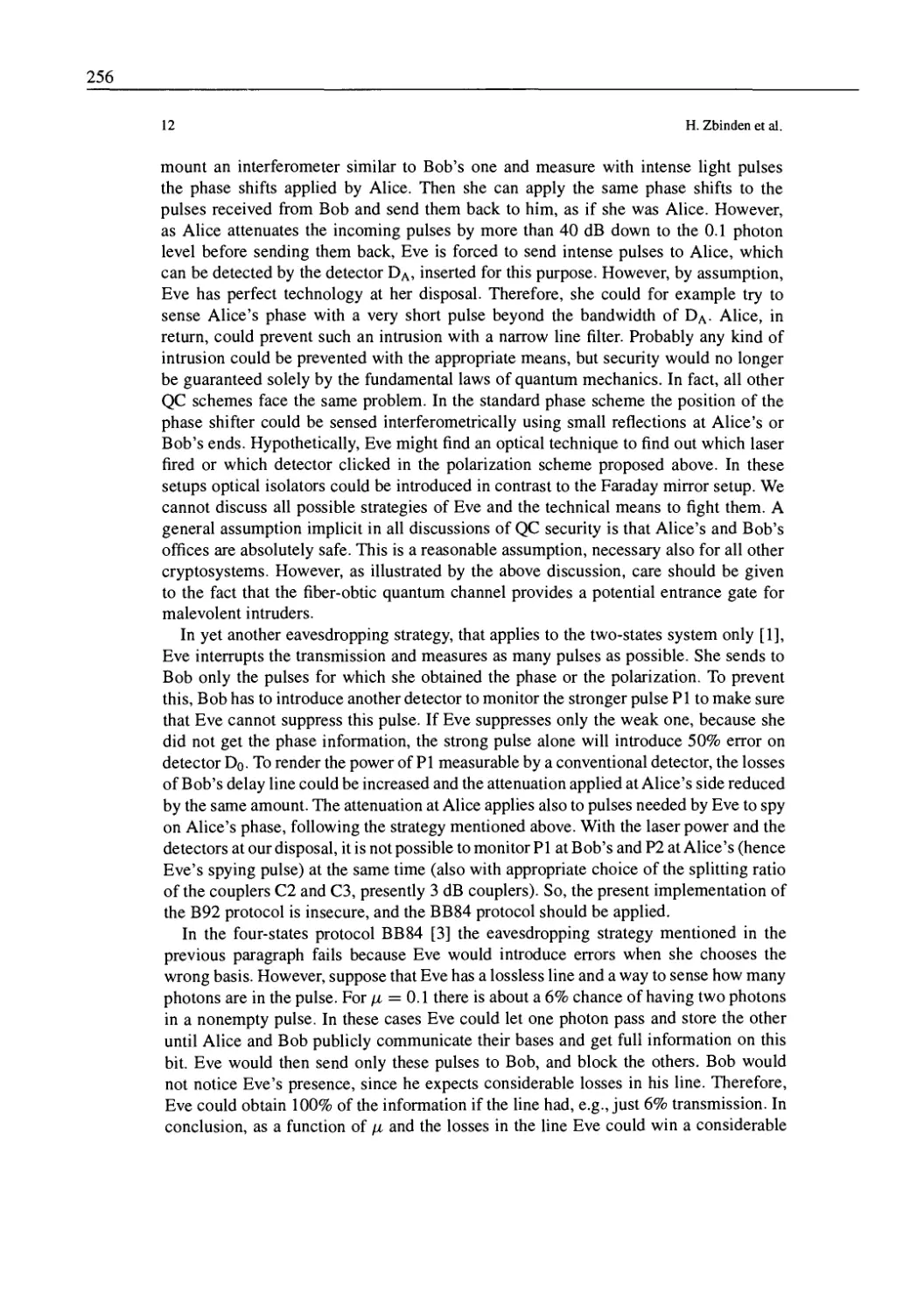
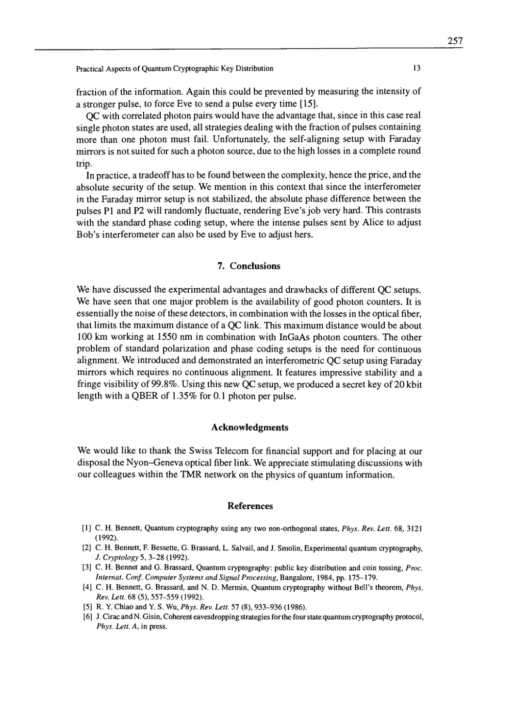
Practical Aspects of Quantum Cryptographic Key Distribution
J. Cryptology 11, 1-14 (1998) 245
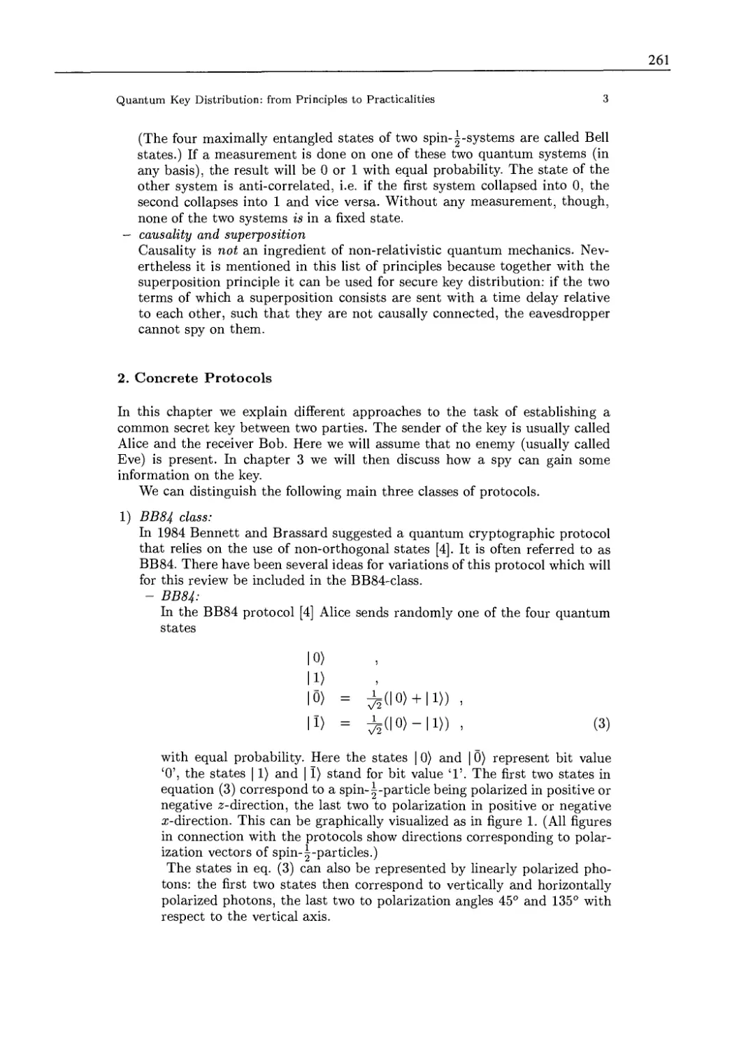
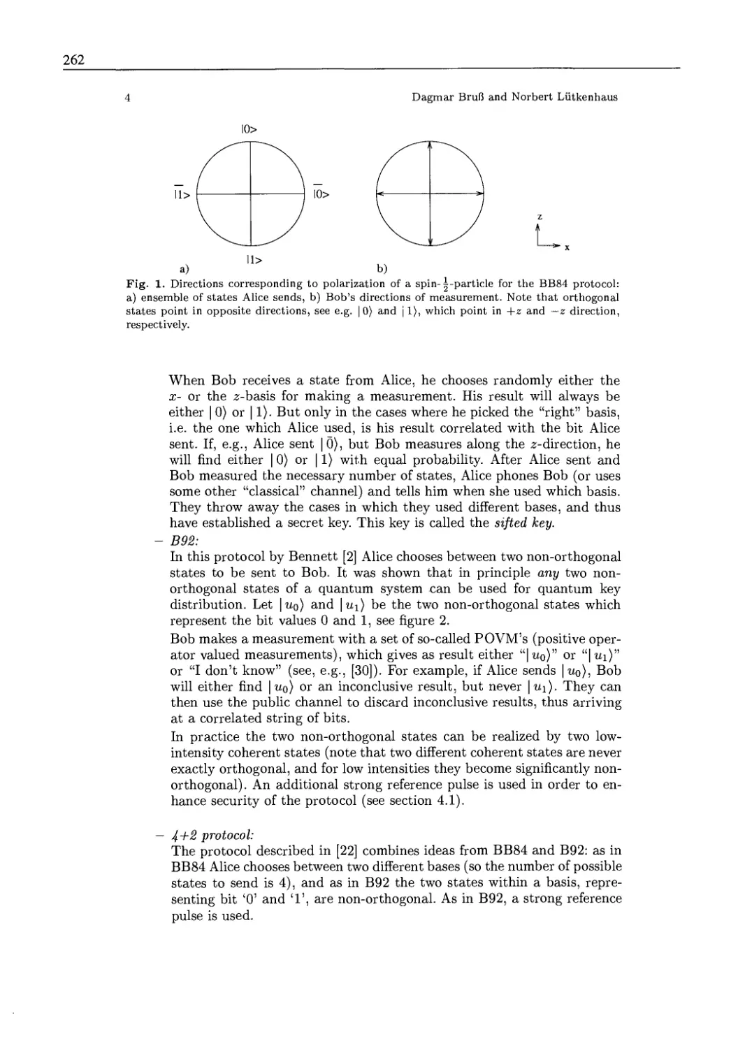
8.3 D. Brufi and N. Liitkenhans
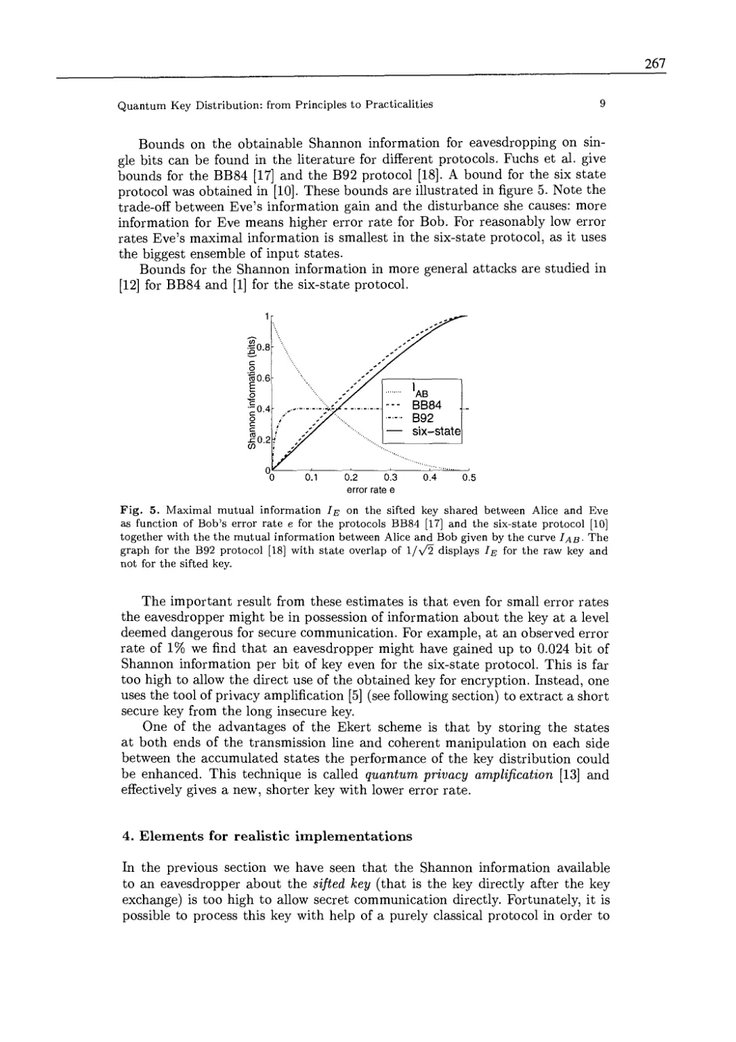
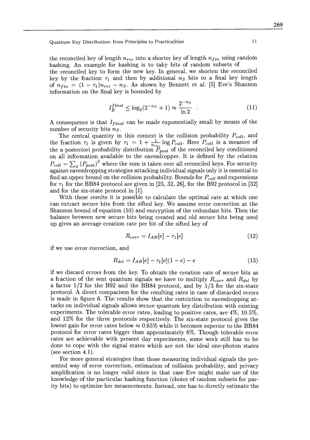
Quantum Key Distribution: From Principles to Practicalities
in Applicable Algebra in Engineering, Communication & Communication 259
Cavity Quantum Electrodynamics 275
9. Cavity Quantum Electrodynamics 277
H. Mabuchi (California Institute of Technology)
9.1 S. Haroche and J. M. Raimond
Cavity Quantum, Electrodynamics
Scientific American (April 1993), p. 26-33 282
9.2 Q. A. Turchette, C. J. Hood, W. Lange, H. Mabuchi and H. J. Kimble
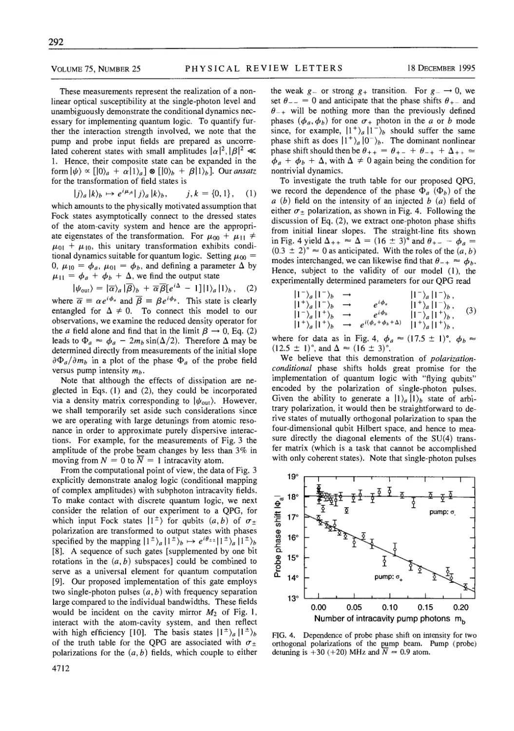
Measurement of Conditional Phase Shifts for Quantum Logic
Phys. Rev. Lett. 75(25), 4710-4713 (1995) 290
9.3 C. J. Hood, M. S. Chapman, T. W. Lynn and H. J. Kimble
Real-Time Cavity QED with Single Atoms
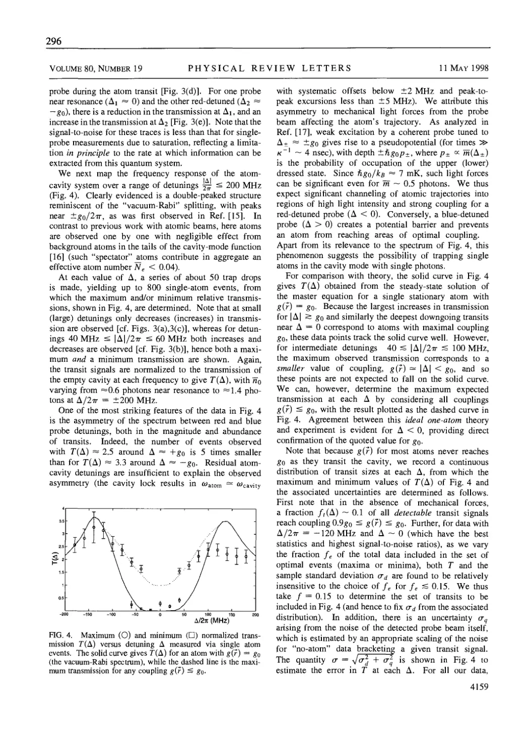
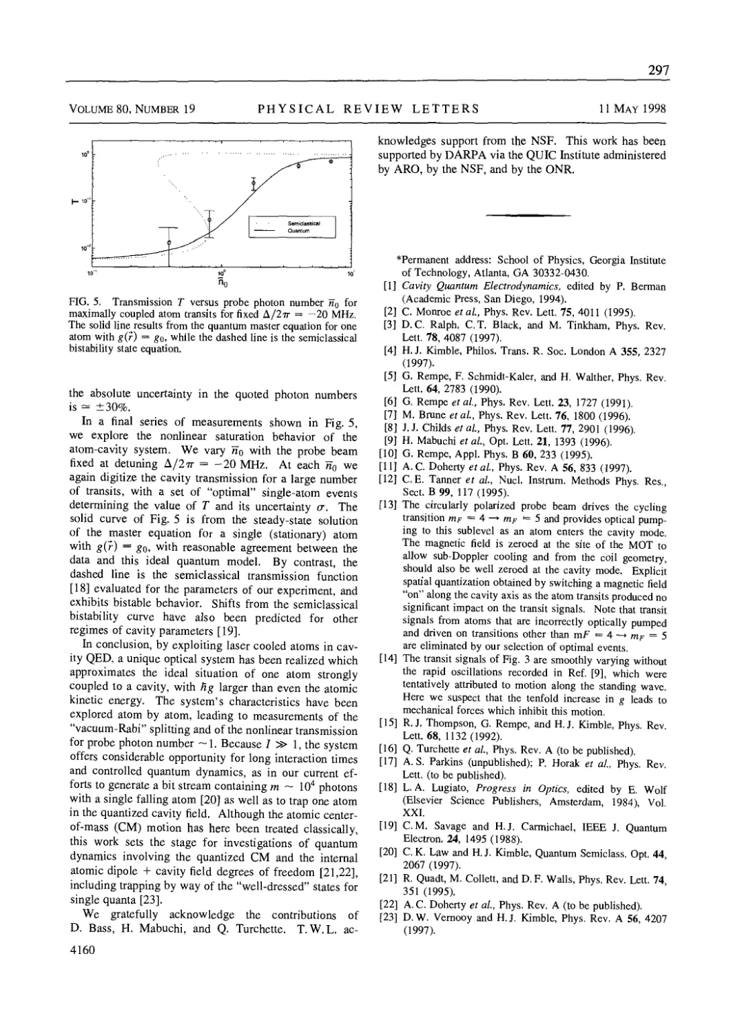
Phys. Rev. Lett. 80(19), 4157-4160 (1998) 294
9.4 X. Maitre, E. Hagley, G. Nogues, C. Wimderklich, P. Goy, M. Bnme,
J. M. Raimond and S. Haroche
Quantum Memory with a Single Photon in a Cavity
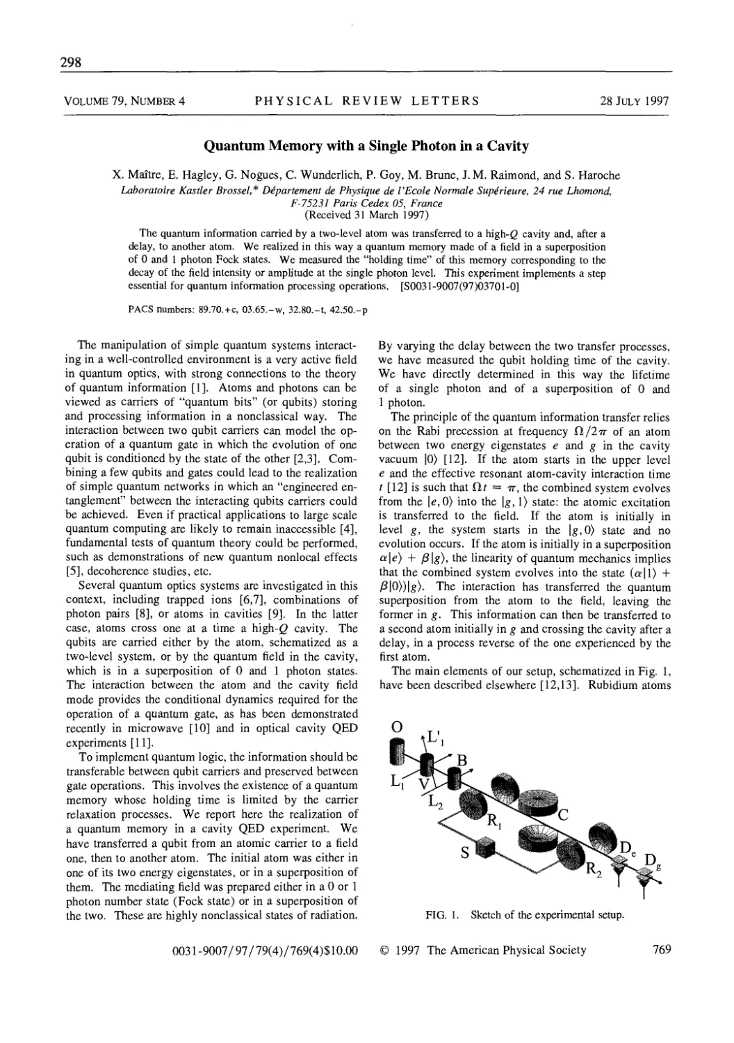
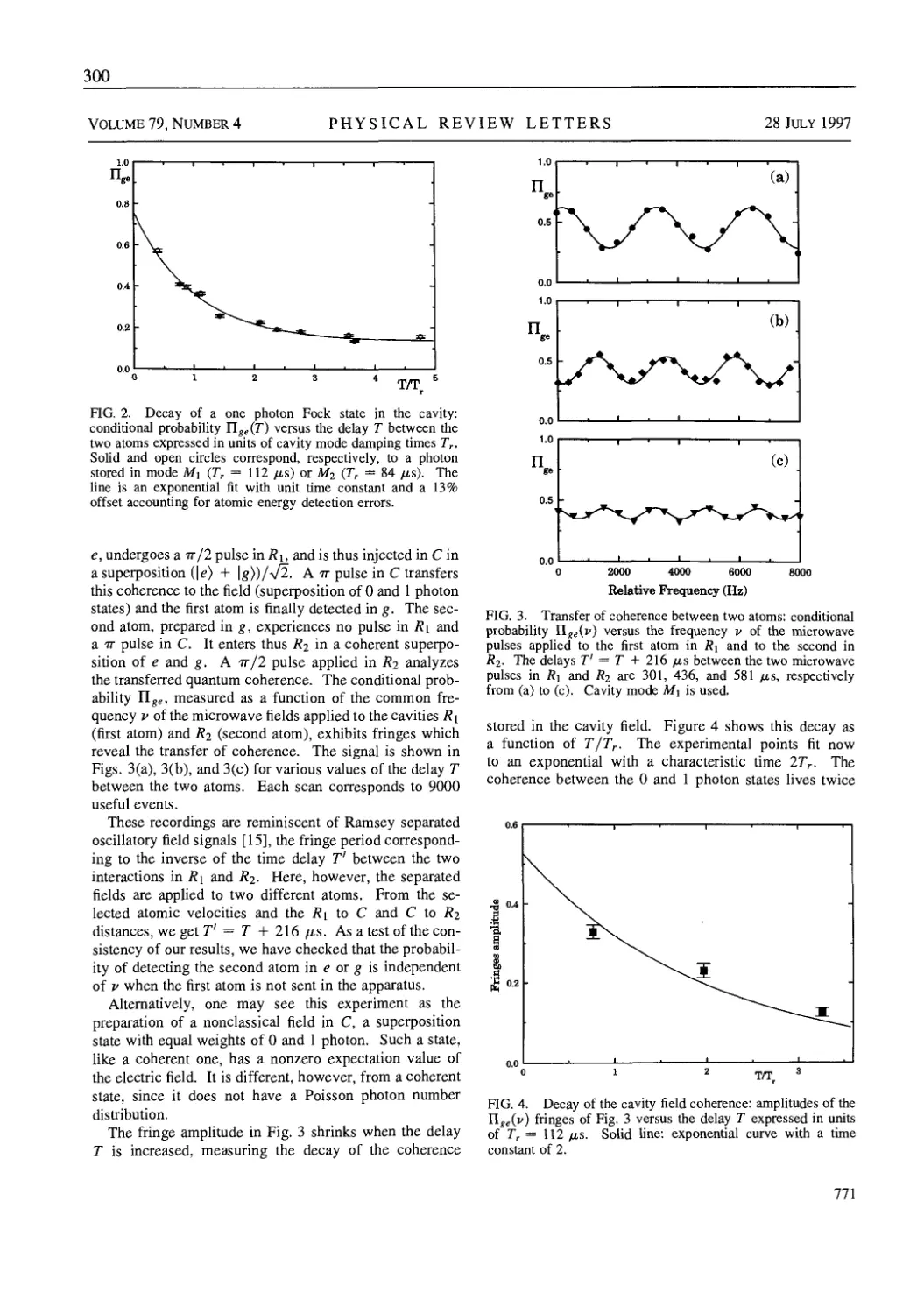
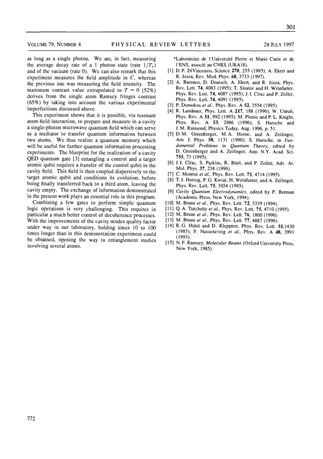
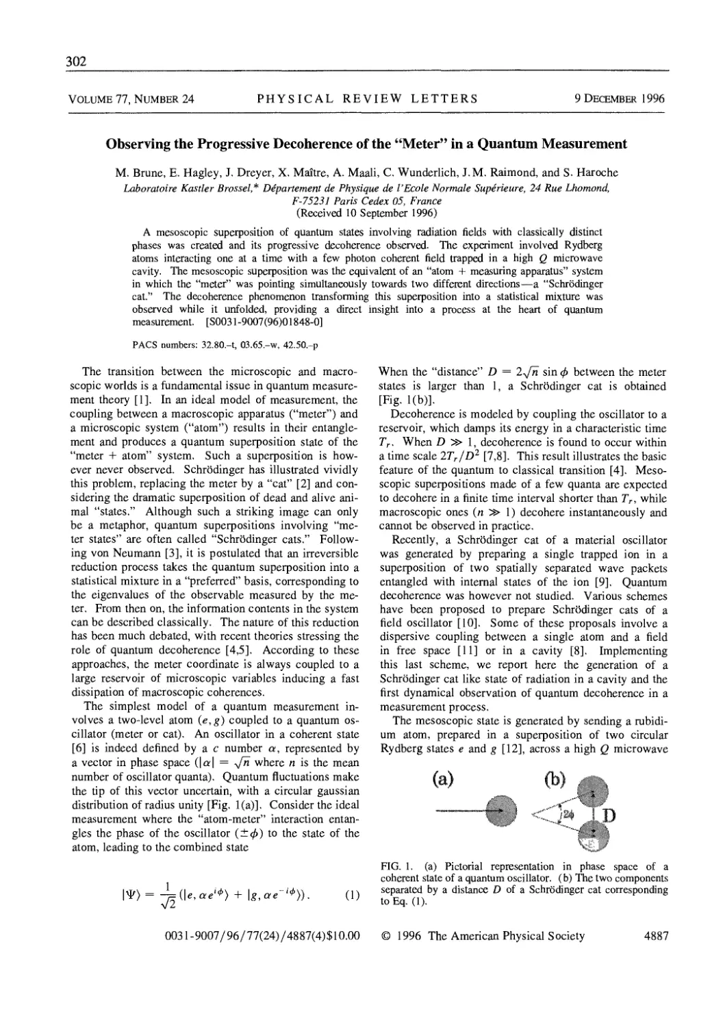
Phys. Rev. Lett. 79(4), 769-772 (1997) 298
9.5 M. Brune, E. Hagley, J. Dreyer, X. Maitre, A. Maali, C. Wunderlich,
J. M. Raimond and S. Haroche
Observing the Progressive Decoherence of the "Meter" in a Quantum
Measurement
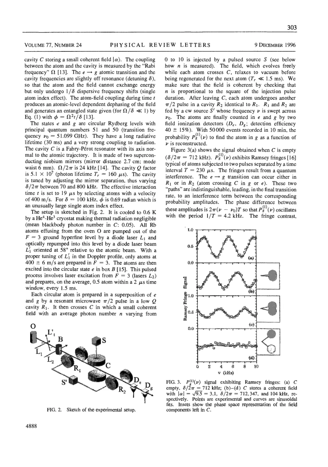
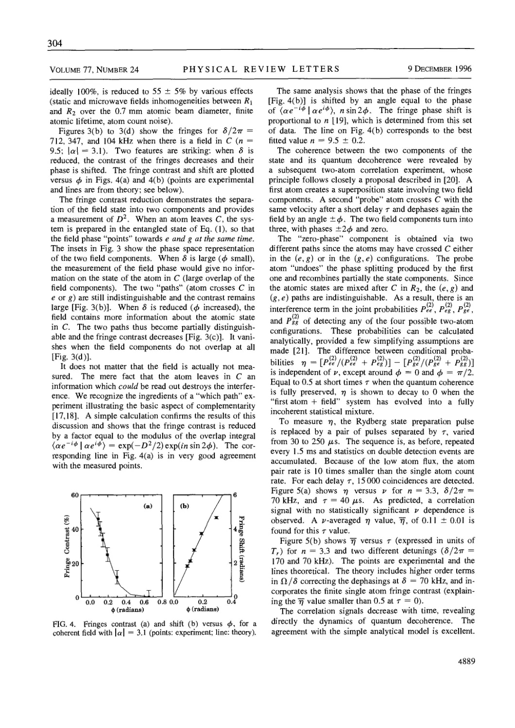
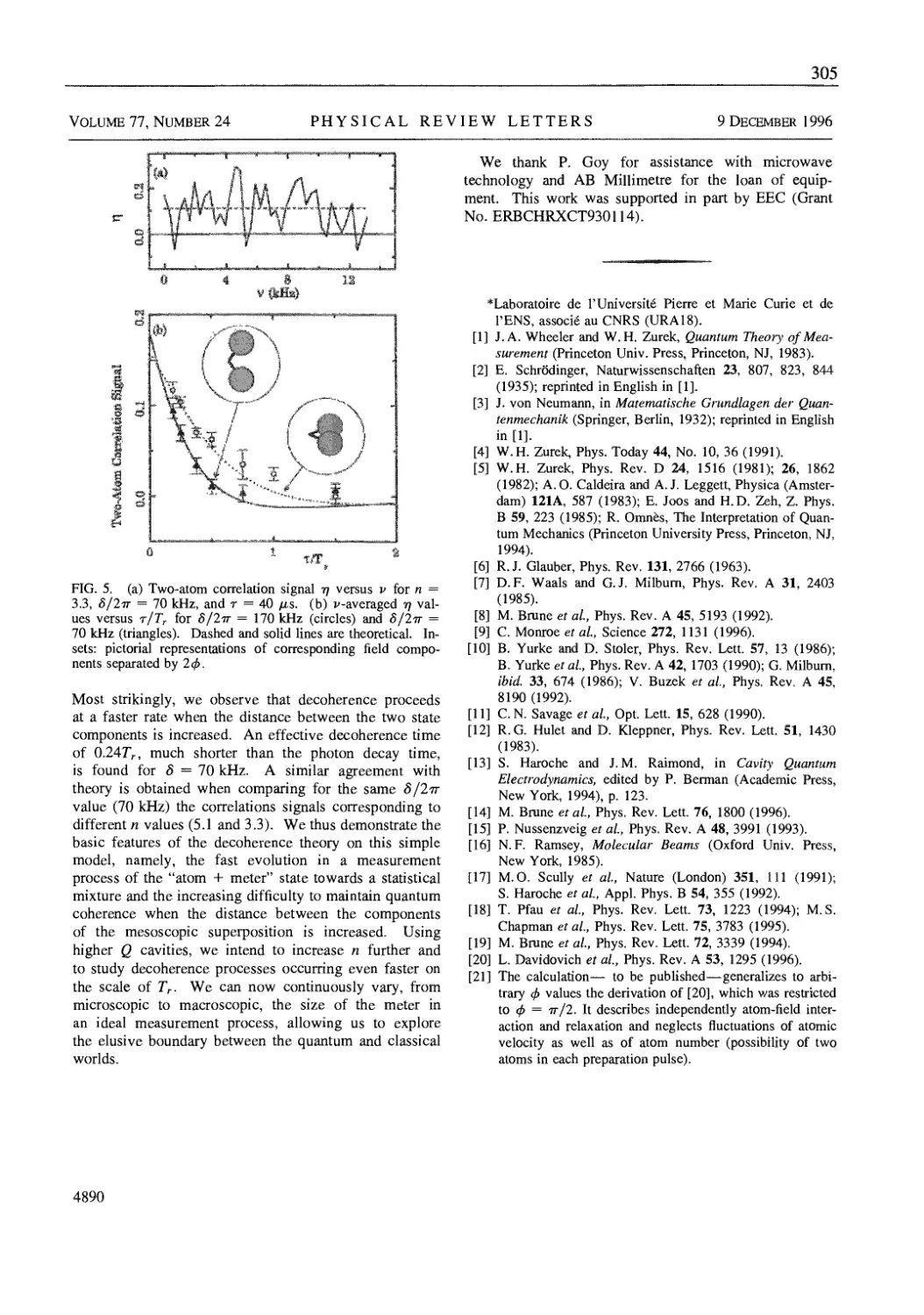
Phys. Rev. Lett. 77(24), 4887-4890 (1996) 302
9.6 H. Mabuchi and P. Zoller
Inversion of Quantum, Jumps in Quantum, Optical Systems under
Continuous Observation
Phys. Rev. Lett. 76(17), 3108-3111 (1996) 306
Quantum Computation with Ion Traps 311
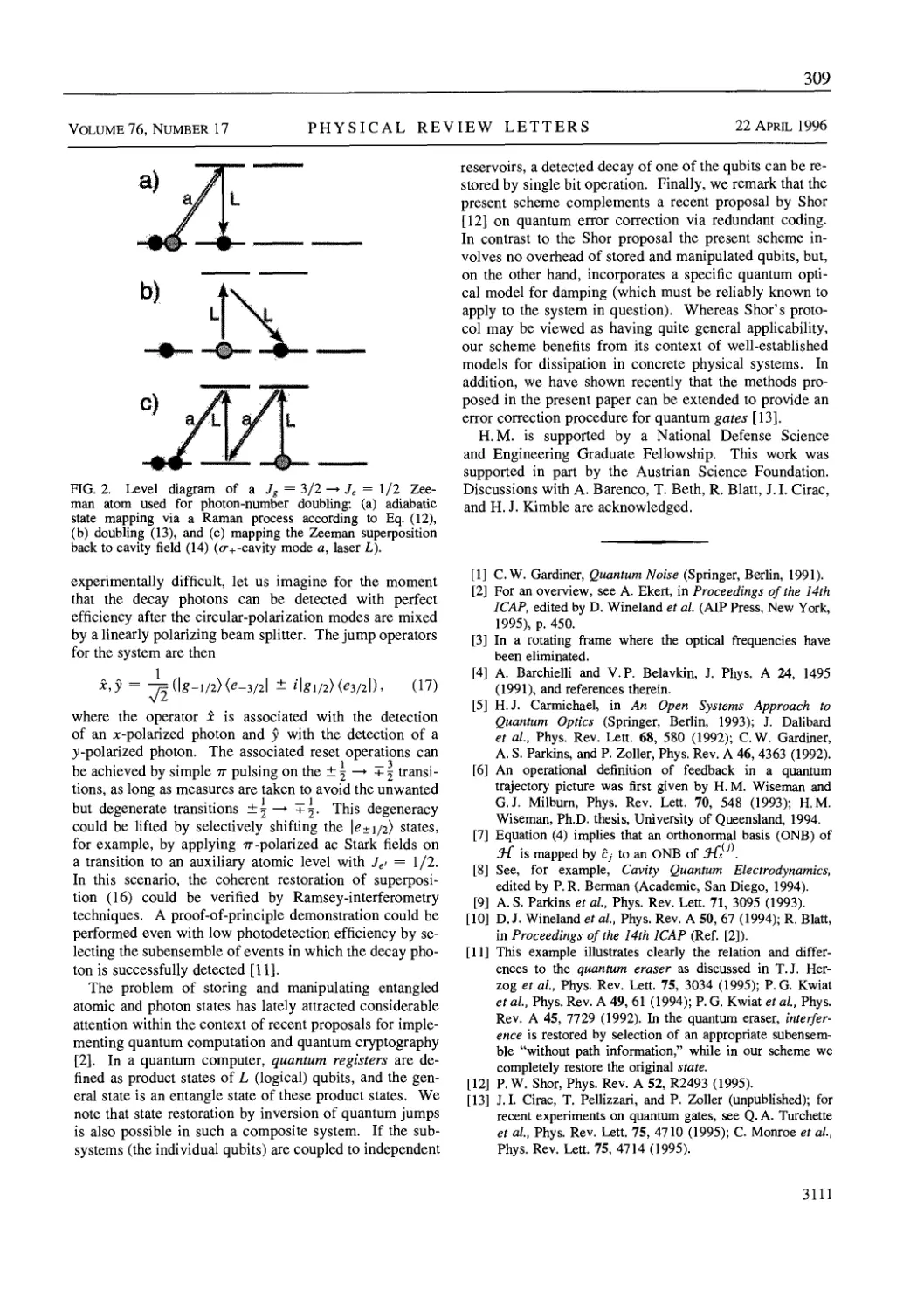
10, Quantum Computation with Ion Traps 313
R. Blatt (University of Innsbruck) &; W. Lange (Max-Planck-Instut
fiir Quantenoptik, Munich)
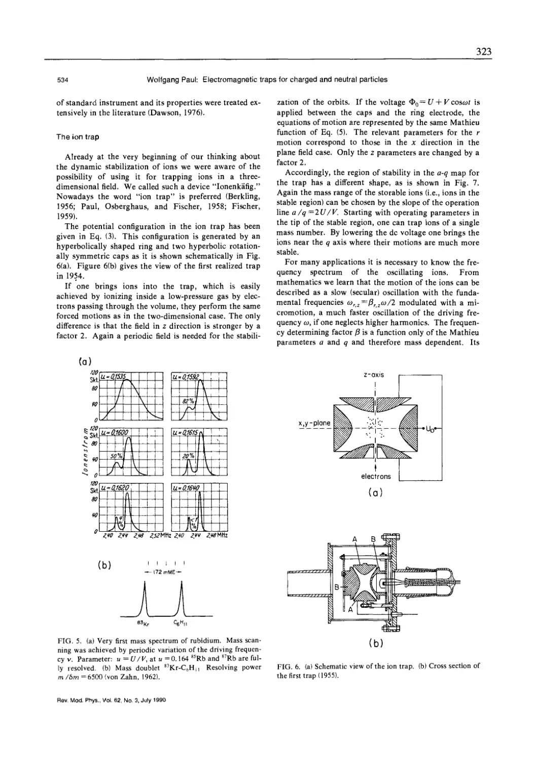
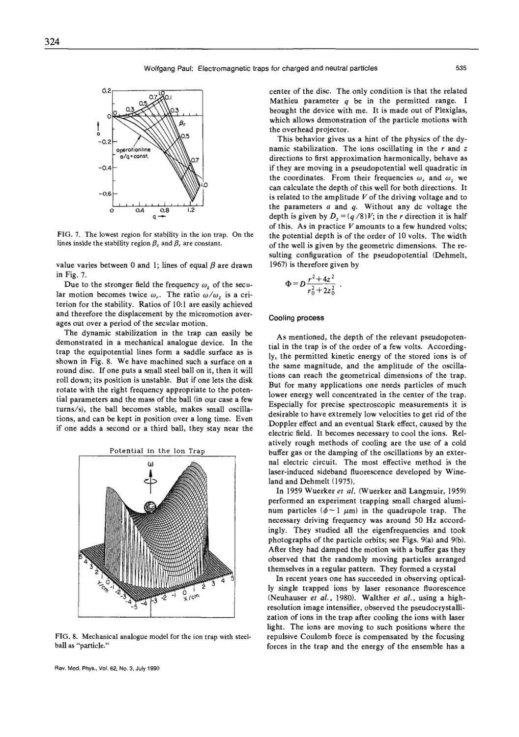
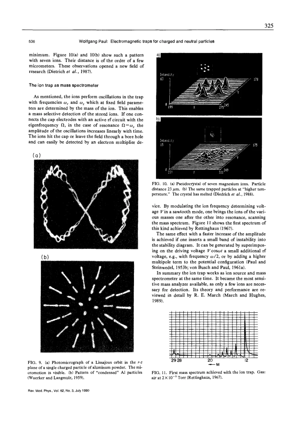
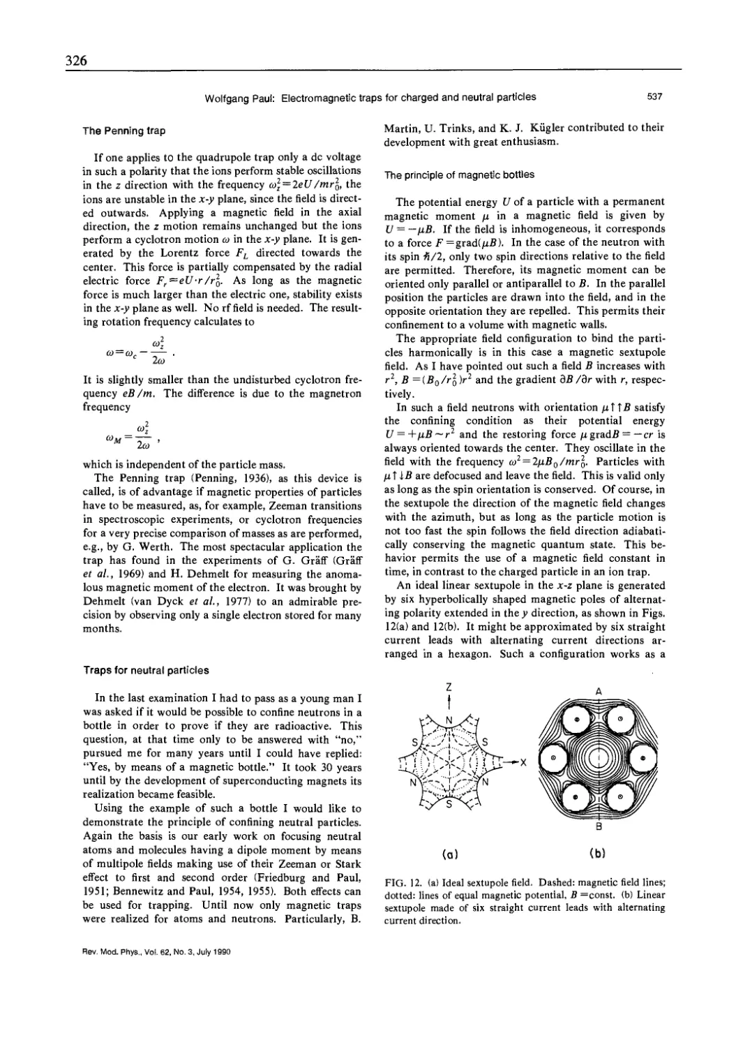
10.1 W. Paul
Electromagnetic Traps for Charged and Neutral Particles
Rev. Mod. Phys. 62(3), 531-540 (1990) 320
10.2 J. I. Cirac and P. Zoller
Quantum Computations with Cold Trapped Ions
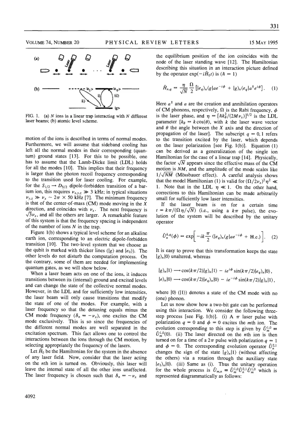
Phys. Rev. Lett. 74(20), 4091-)-4094 (1995) 330
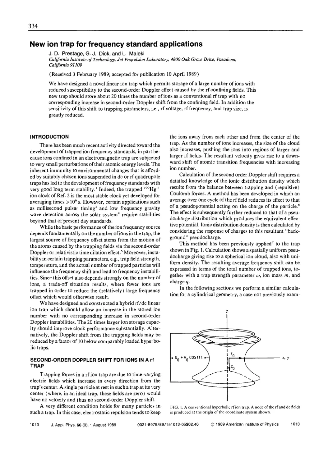
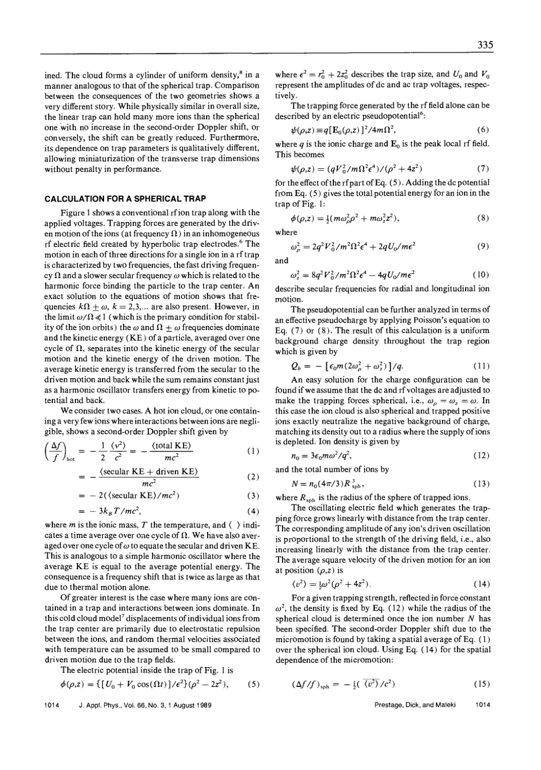
10.3 J. D. Prestage, G. J. Dick and L. Maleki
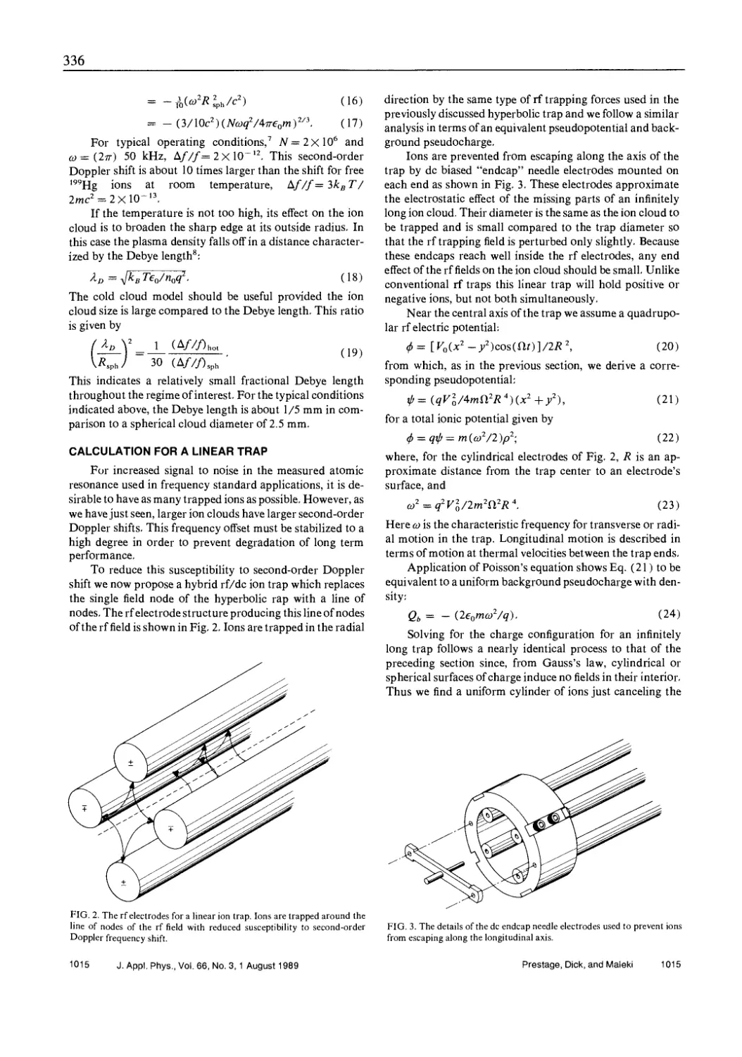
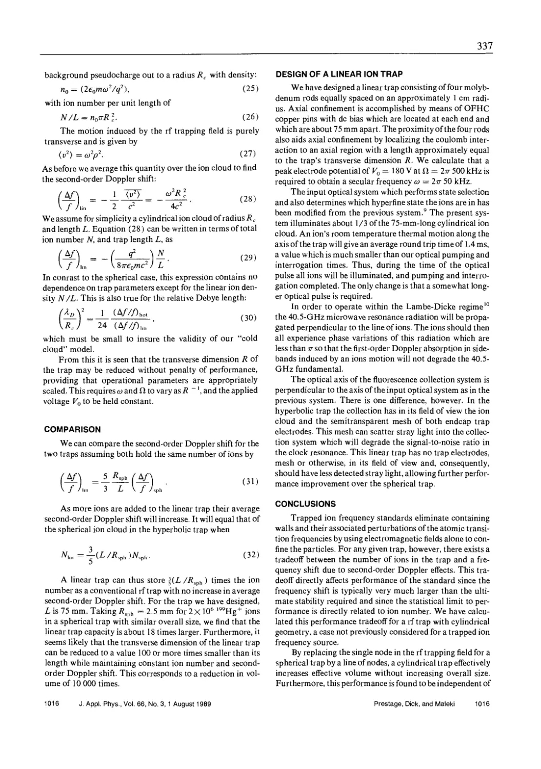
New Ion Trap for Frequency Standard Applications
J. Appl. Phys. 66(3), 1013-1017 (1989) 334
XI
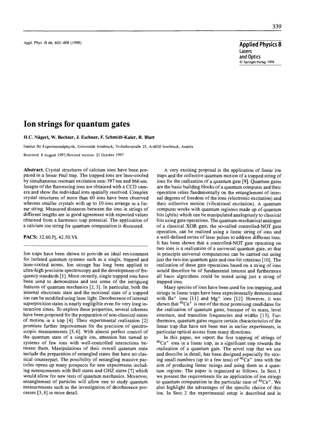
10.4 H. C. Nagerl, W. Bechter, J. Eschner, F. Schmidt-Kaler and R. Blatt
Ion Strings for Quantum Gates
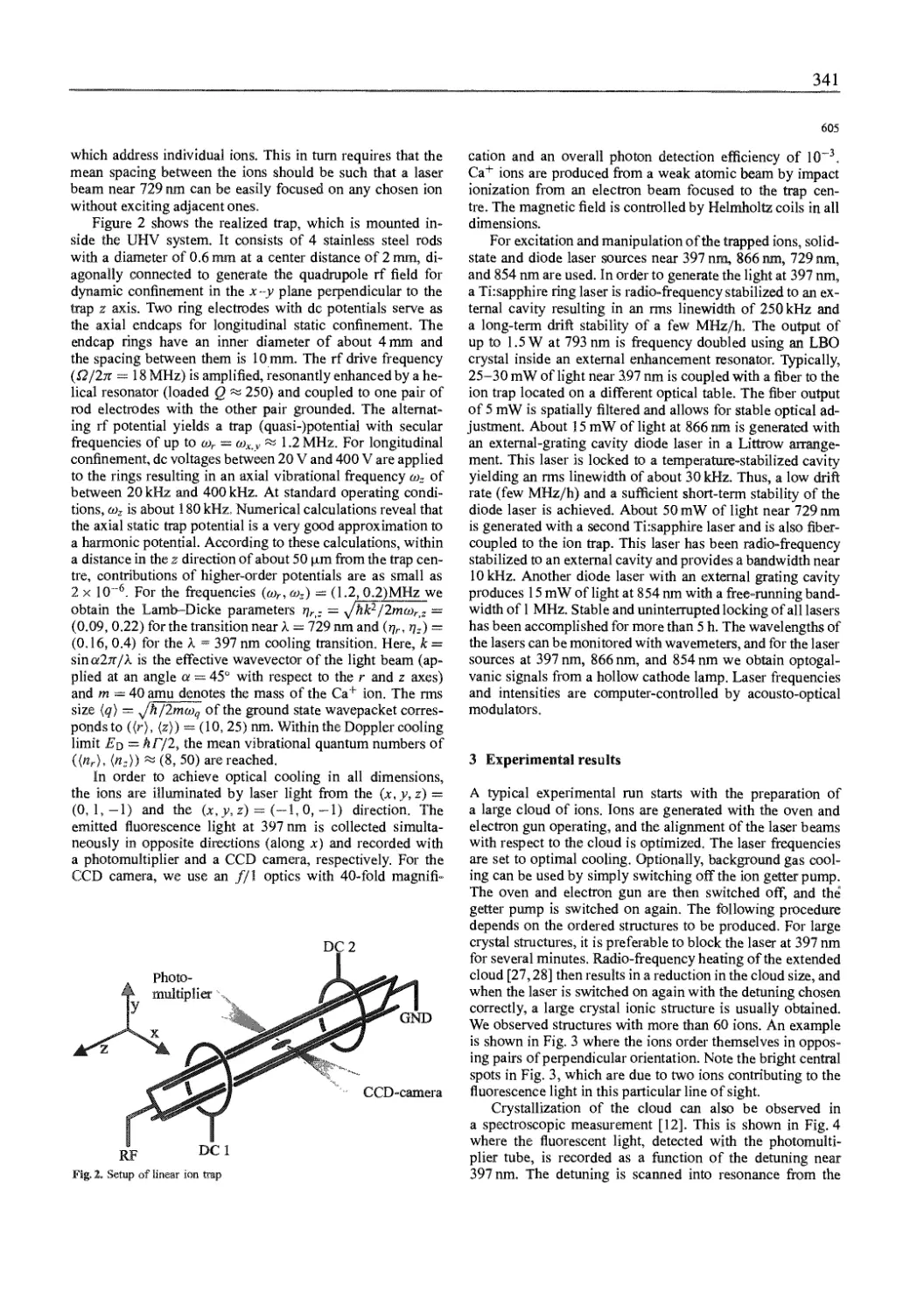
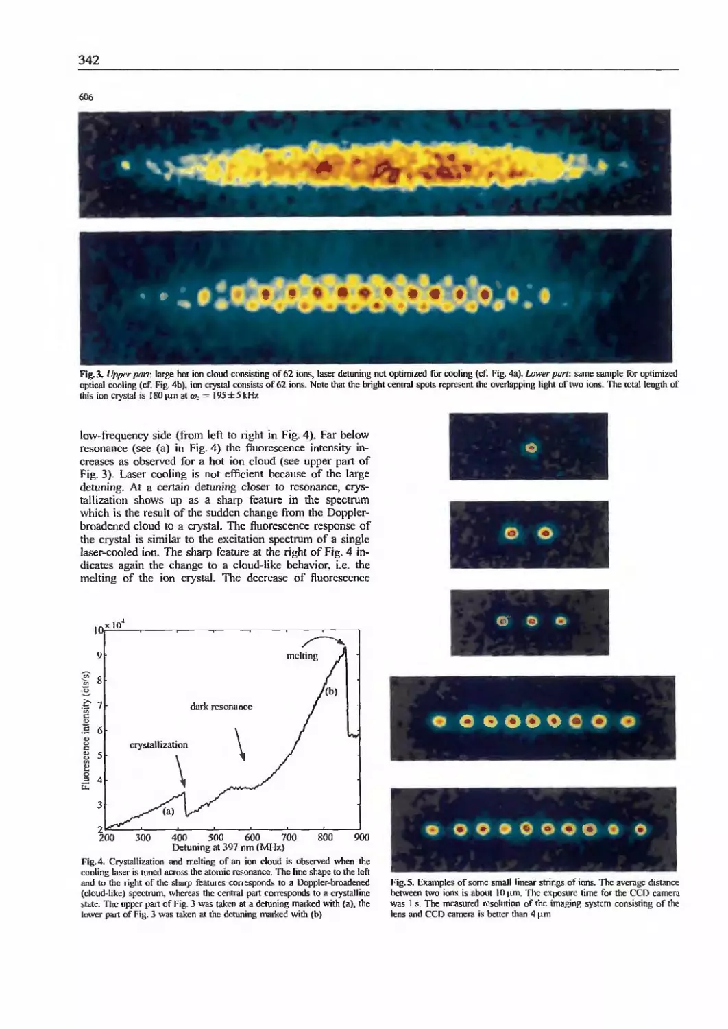
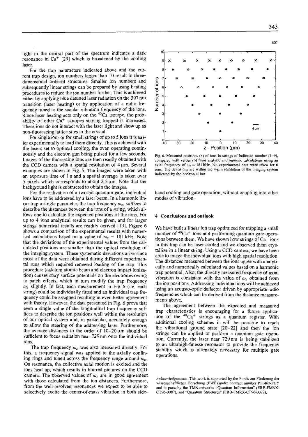
Appl. Phys. B " Lasers Opt. 66, 603-608 (1998) 339
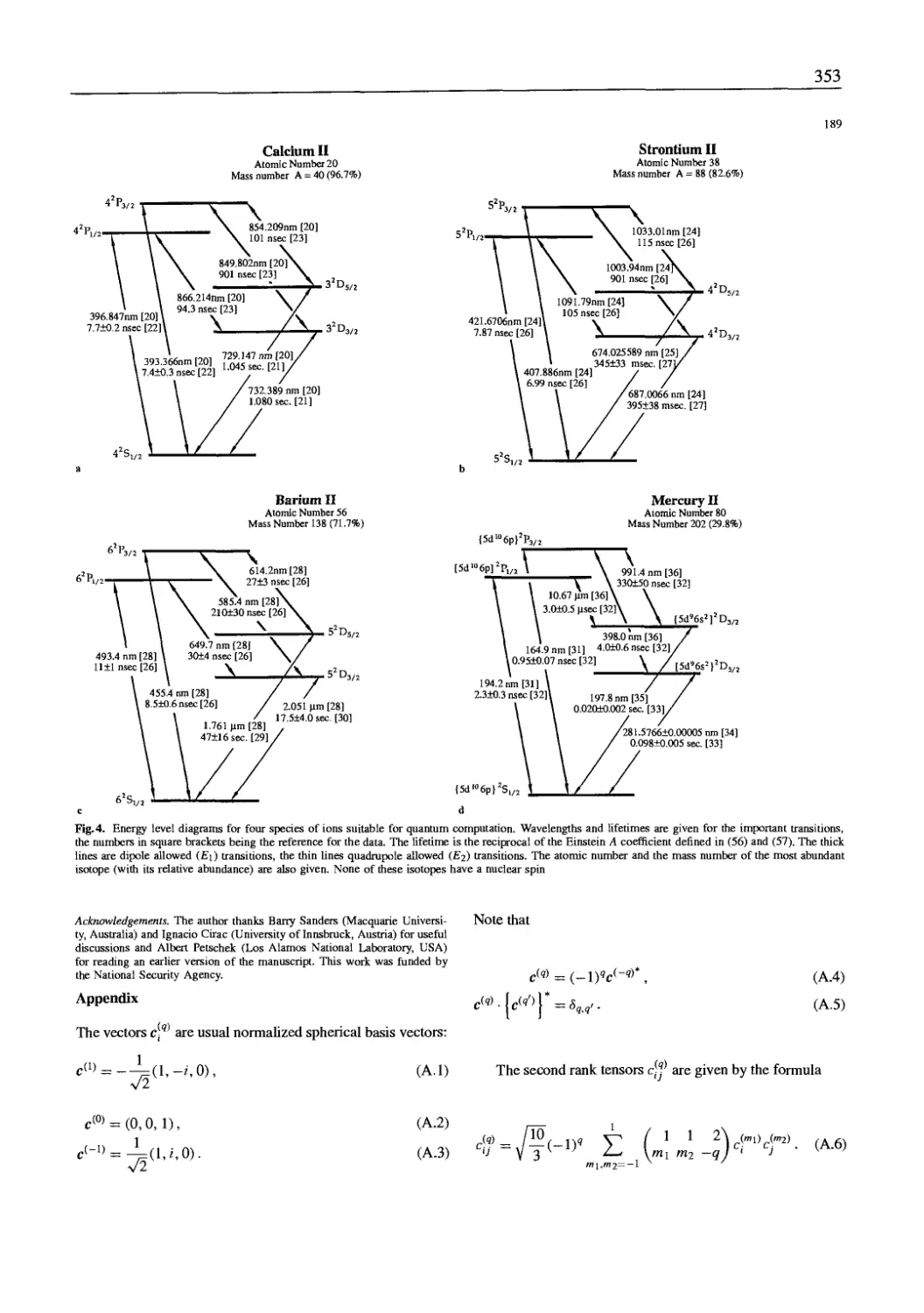
10.5 D. F. V. James
Quantum Dynamics of Cold Trapped Ions with Application to Quantum.
Computation
AppL Phys. B - Lasers Opt. 66, 181-190 (1998) 345
10.6 C. Monroe, D. M. Meekhof, B. E. King, W. M. Itano and D. J. Wineland
Demonstration of a Fundamental Quantum Logic Gate
Phys. Rev. Lett. 75(25), 4714-4717 (1995) 355
10.7 Q. A. Turchette, C. S. Wood, B. E. King, C. J. Myatt, D. Leibfried,
W. M. Itano, C. Monroe and D. J. Wineland
Deterministic Entanglement of Two Trapped Ions
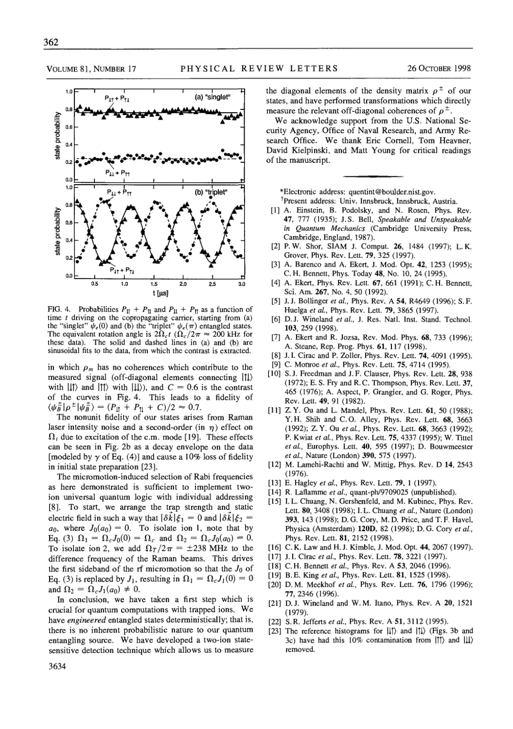
Phys. Rev. Lett. 81(17), 3631-3614 (1998) 359
Josephson Junctions and Quantum Computation 363
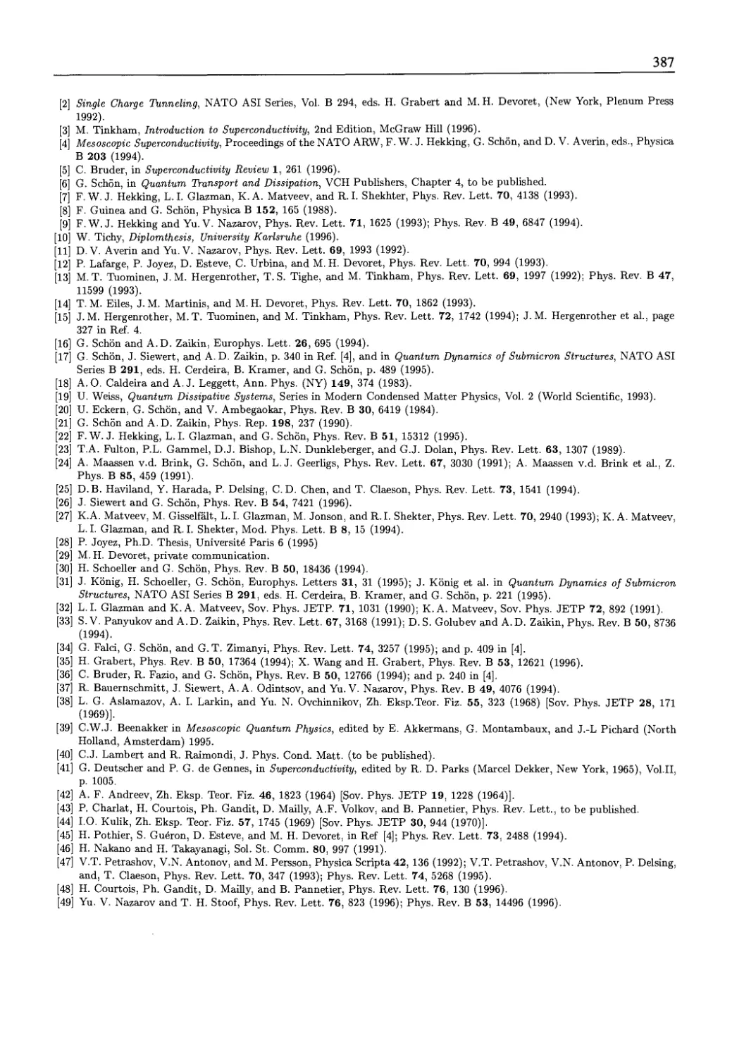
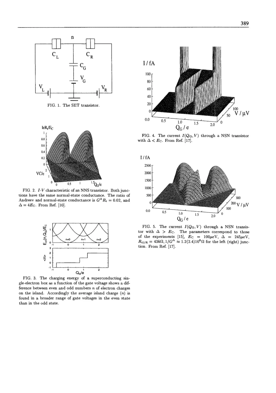
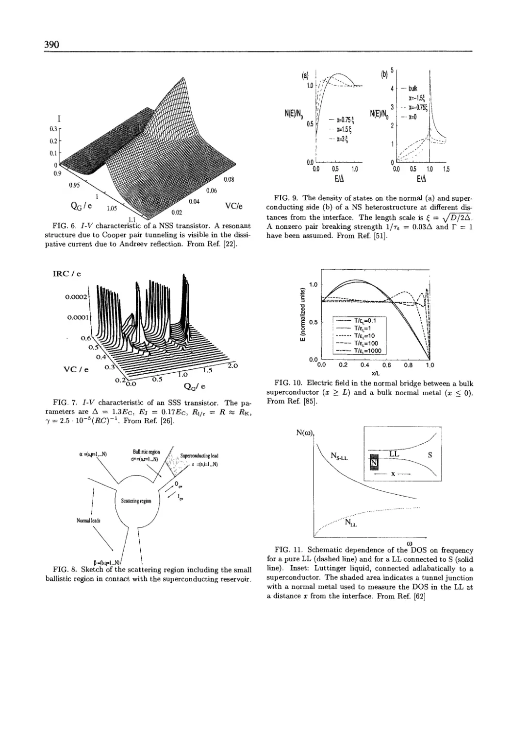
11. Josephson Junctions and Quantum Computation 365
R. Fazio (University of Catania) &; G. Schon (University of Karlsruhe)
11.1 R. Fazio and G. Schon
Mesoscopic Effects in Superconductivity
in Mesoscopic Electron Transport, NATO ASI series E, 345, 407, Kluver (1997) 368
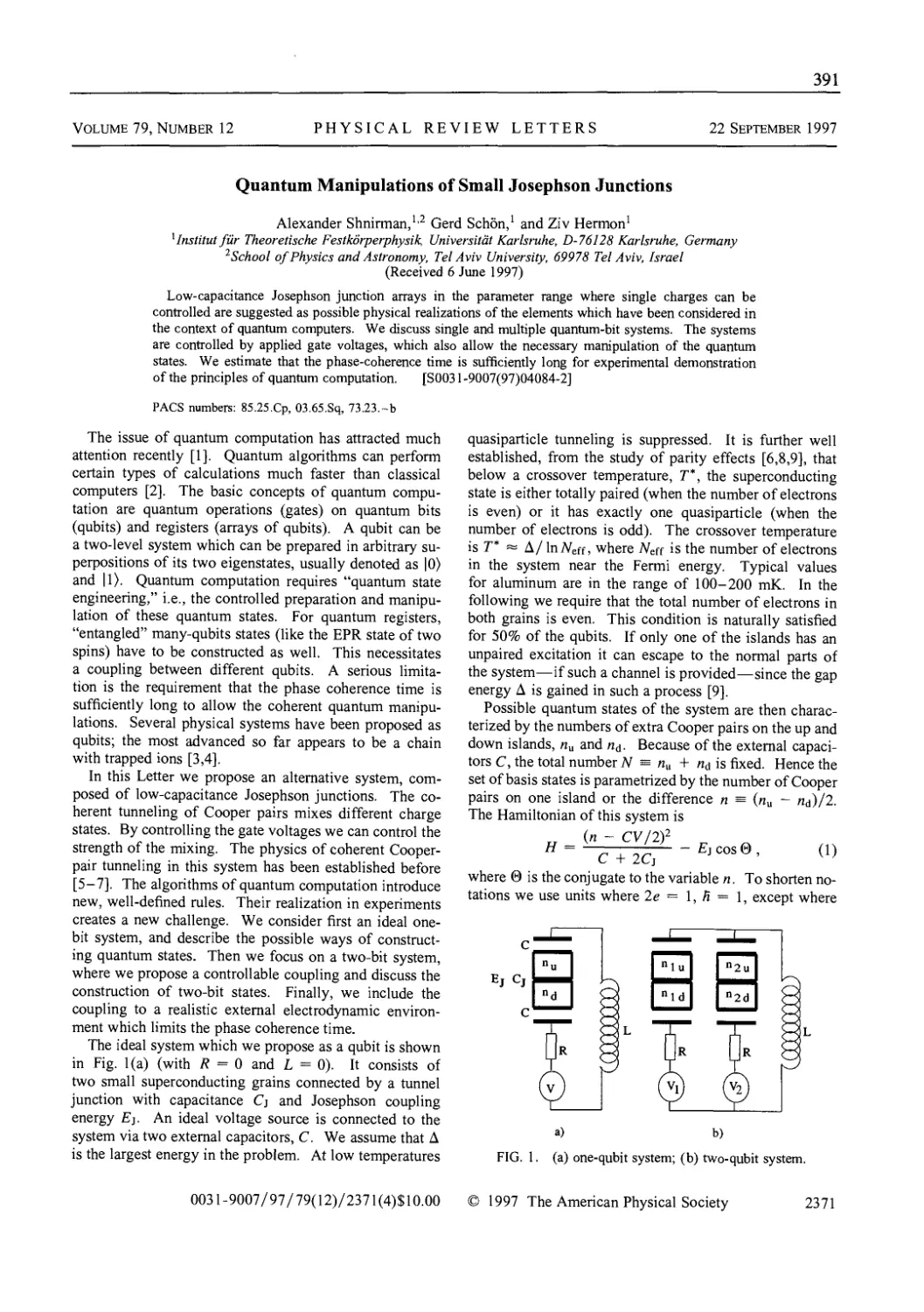
11.2 A. Shnirman, G. Schon and Ziv Hermon
Quantum, Manipulations of Small Josephson Junctions
Phys. Rev. Lett. 79(12), 2371-2374 (1997) 391
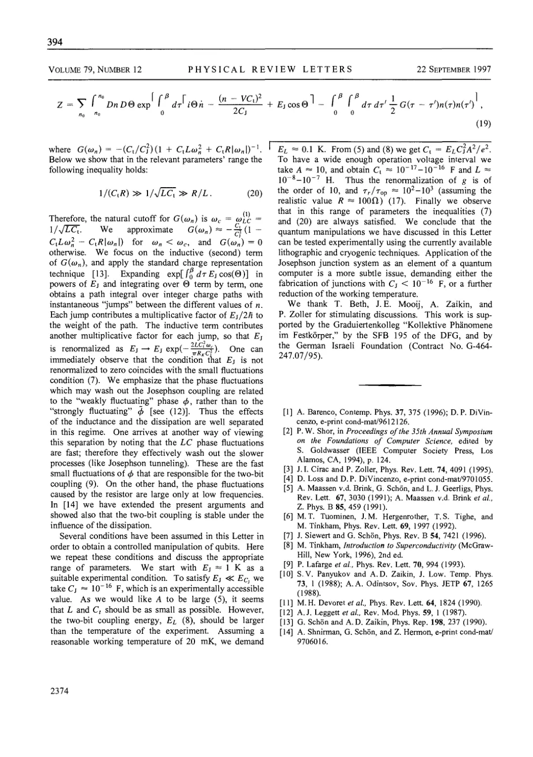
11.3 Y. Makhlin, G. Schon and A. Shnirman
Josephson-Junction Qubits with Controlled Couplings
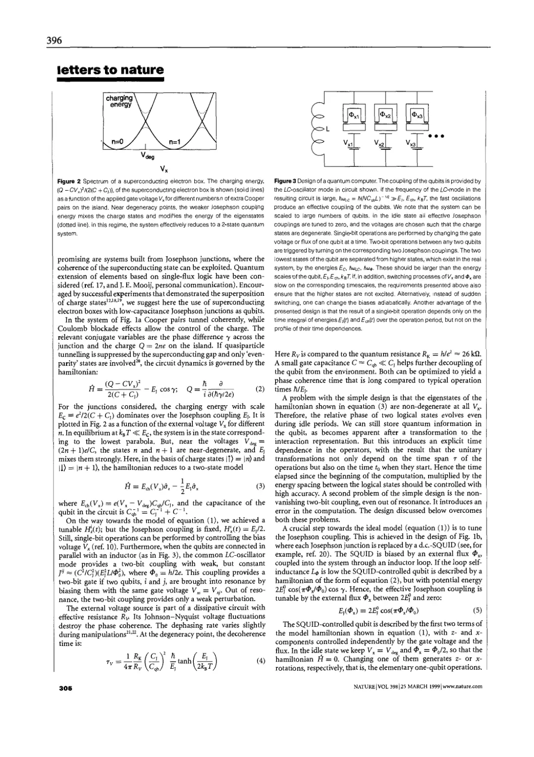
Nature, 398, 305-307 (1999) 395
Quantum Computing in Optical Lattices 399
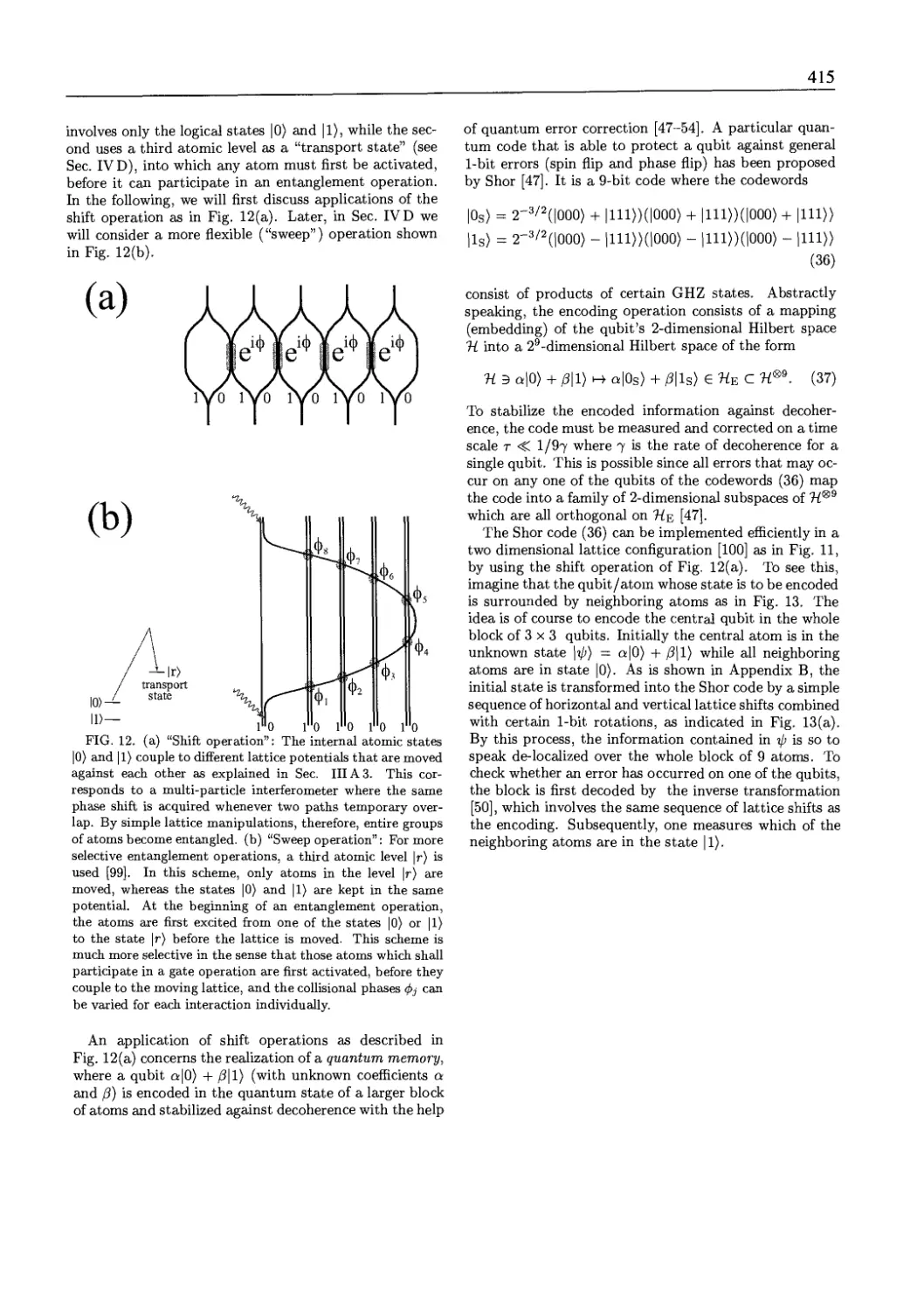
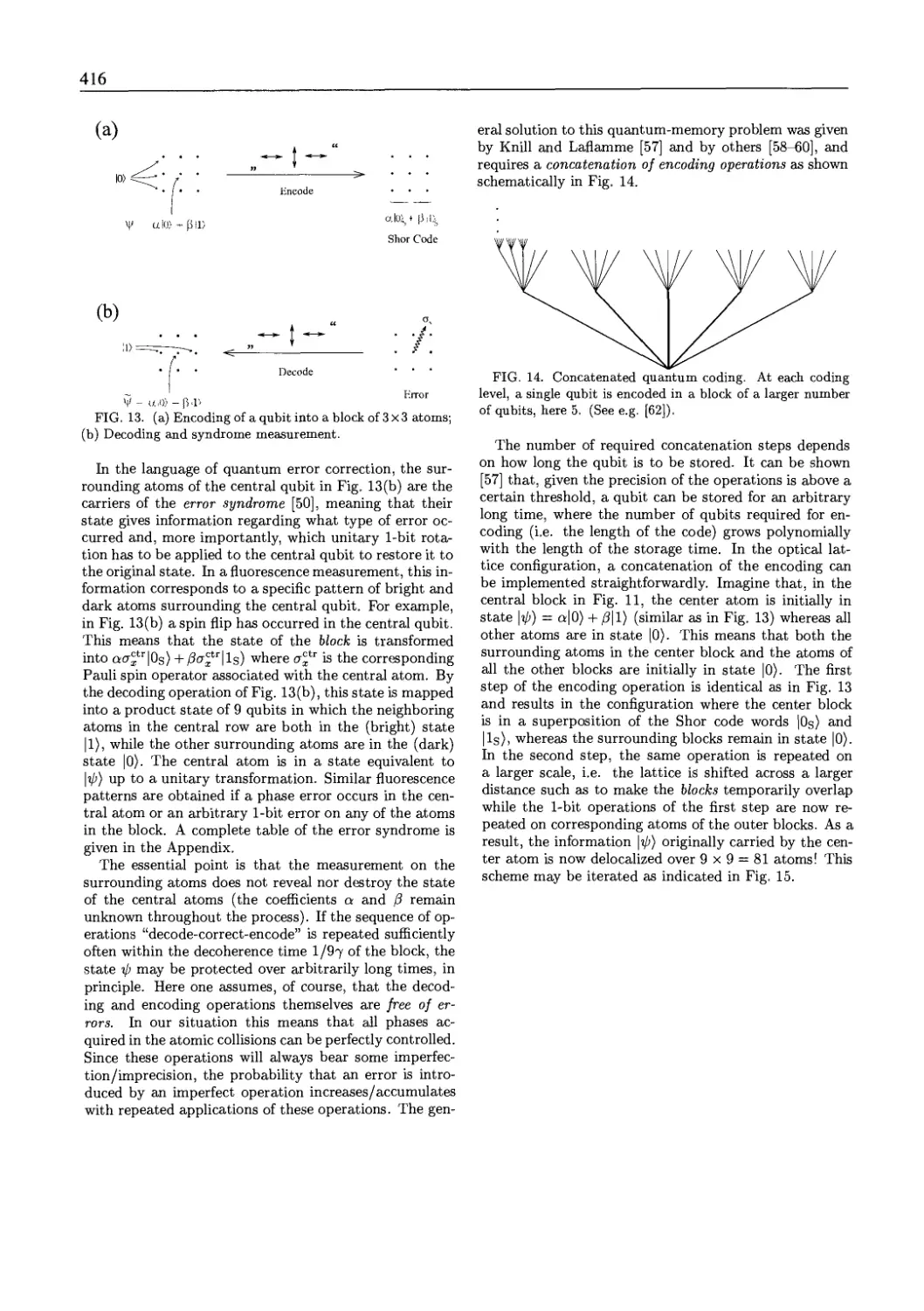
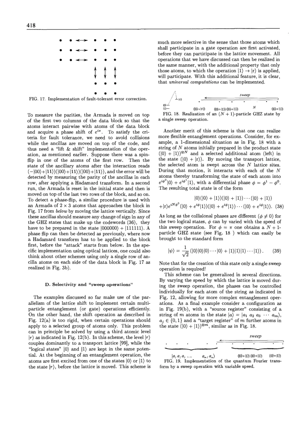
12. Quantum Information in Optical Lattices 401
H. Briegel (Ludwig-Maximilians-Universitaet, Munich)
12.1 H.-J. Briegel, T. Calarco, D. Jaksch, J. L Cirac and P. Zoller
Quantum Computing with Neutral Atoms
Reprint, to appear in the special issue of J. Mod. Opt. (2000) on The Physics
of Quantum Information 404
Quantum Computation and Quantum Communication
with Electrons 425
13. Quantum Computation and Quantum Communication with Electrons 427
D. Loss (University of Basel)
13.1 D. Loss and D. P. DiVincenzo
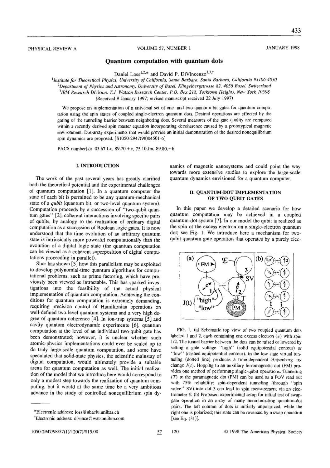
Quantum Computation with Quantum Dots
Phys. Rev. A 57(1), 120-126 (1998) 433
Xll
13.2 G. Burkard, D. Loss and D. P. DiVincenzo
Coupled Quantum Dots as Quantum Gates
Phys. Rev. B 59(3), 2070-2078 (1999) 440
13.3 D. P, DiVincenzo and D. Loss
Quantum Computers and Quantum Coherence
J. Magn. Magn. Matler. 200 special issue on Magnetism beyond 2000
also cond-mat/9901137 449
NMR Quantum Computing 463
14, Quantum Computing with NMR 465
J. Jones (Oxford University)
14.1 D. G. Cory, A. F. Fahmy and T. F. Havel
Nuclear Magnetic Resonance Spectroscopy: An Experimentally Accessible
Paradigm for Quantum Computing
Proceedings of PhysComp '96 (eds. T. Toffoli, M. Biafore and J. Leao),
(New England Complex Systems Institute, 1996) pp. 87-91 471
14.2 J. A. Jones and M. Mosca
Implementation of a Quantum, Algorithm, on a Nuclear Magnetic Resonance
Quantum, Computer
J. Chem. Phys. 109(5), 1648-1653 (1998) 476
14.3 L L. Chuang, N, Gershenfeld and M. Kubinec
Experimental Implementation of Fast Quantum Searching
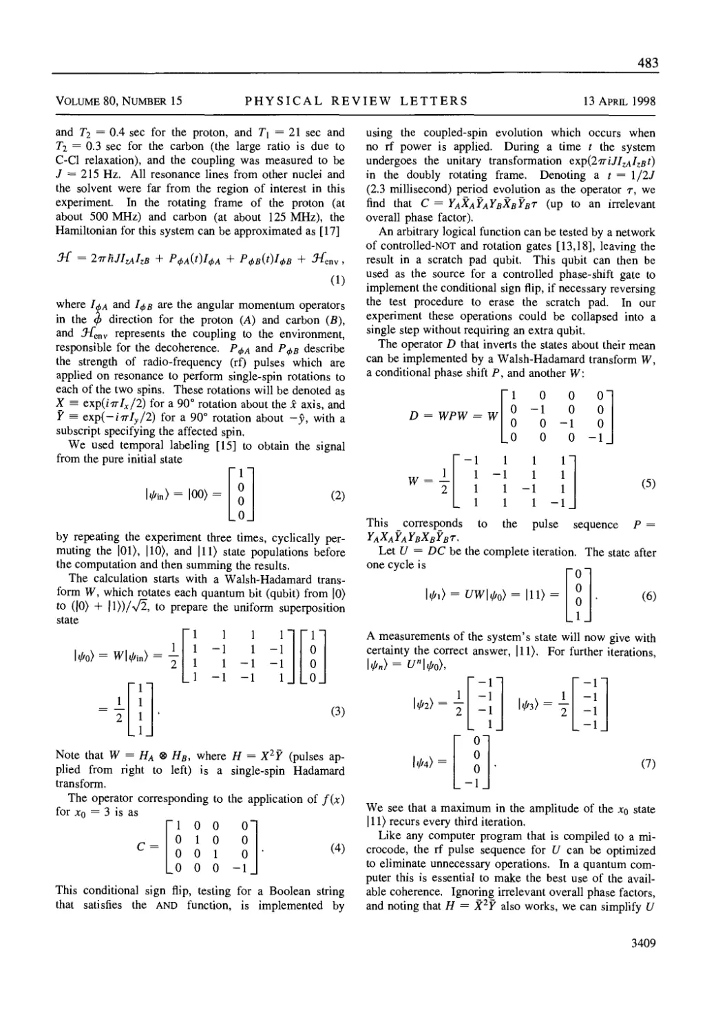
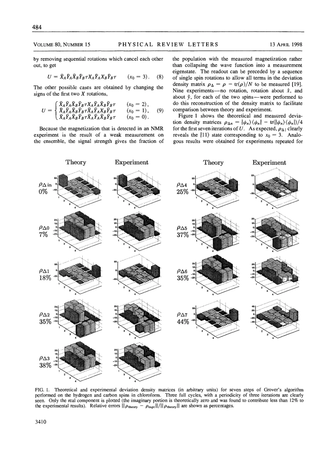
Phys, Rev. Lett. 80(15), 3408-3411 (1998) 482
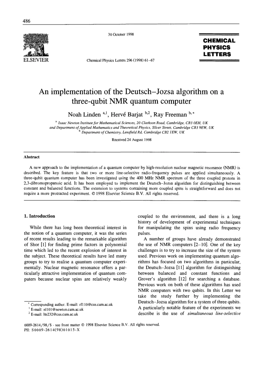
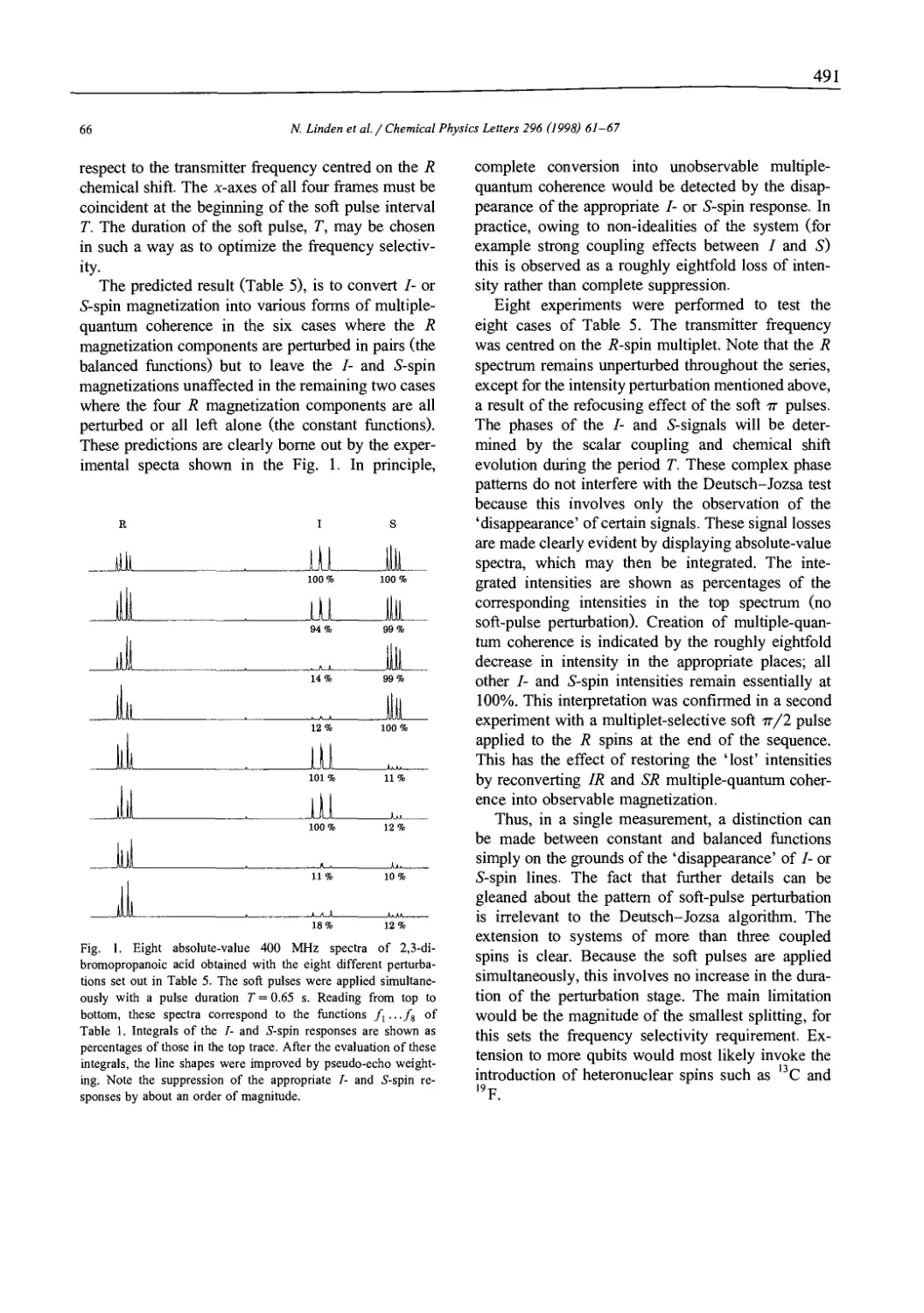
14.4 N. Linden, H. Barjat and R. Freeman
An Implementation of the Deutsch-Jozsa Algorithm on a Three-Qubit NMR
Quantum Computer
Chem. Phys. Lett. 296, 61-67 (1998) 486
Selected Bibliography 493
Introductory Concepts
Introductory Concepts
Anton Zeilinger
University of Vienna
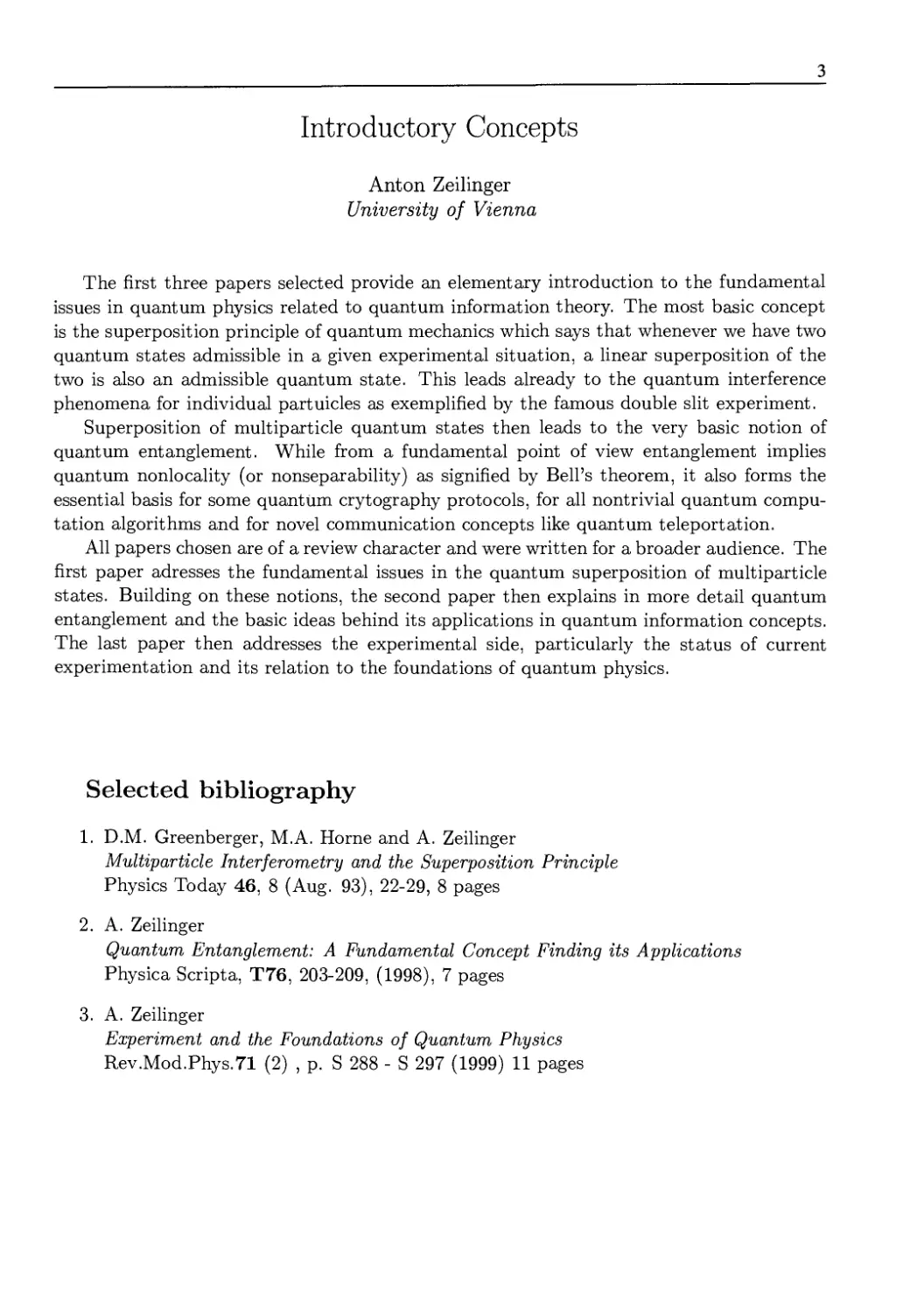
The first three papers selected provide an elementary introduction to the fundamental
issues in quantum physics related to quantum information theory. The most basic concept
is the superposition principle of quantum mechanics which says that whenever we have two
quantum states admissible in a given experimental situation, a linear superposition of the
two is also an admissible quantum state. This leads already to the quantum interference
phenomena for individual partuicles as exemplified by the famous double slit experiment.
Superposition of multiparticle quantum states then leads to the very basic notion of
quantum entanglement. While from a fundamental point of view entanglement implies
quantum nonlocality (or nonseparability) as signified by Bell's theorem, it also forms the
essential basis for some quantum crytography protocols, for all nontrivial quantum
computation algorithms and for novel communication concepts like quantum teleportation.
All papers chosen are of a review character and were written for a broader audience. The
first paper adresses the fundamental issues in the quantum superposition of multiparticle
states. Building on these notions, the second paper then explains in more detail quantum
entanglement and the basic ideas behind its applications in quantum information concepts.
The last paper then addresses the experimental side, particularly the status of current
experimentation and its relation to the foundations of quantum physics.
Selected bibliography
1. D,M. Greenberger, M.A. Home and A. Zeilinger
Multiparticle Interferometry and the Superposition Principle
Physics Today 46, 8 (Aug. 93), 22-29, 8 pages
2. A. Zeilinger
Quantum Entanglement: A Fundamental Concept Finding its Applications
Physica Scripta, T76, 203-209, (1998), 7 pages
3. A. Zeilinger
Experiment and the Foundations of Quantum Physics
Rev,Mod.Phys.71 (2) , p, S 288 - S 297 (1999) 11 pages
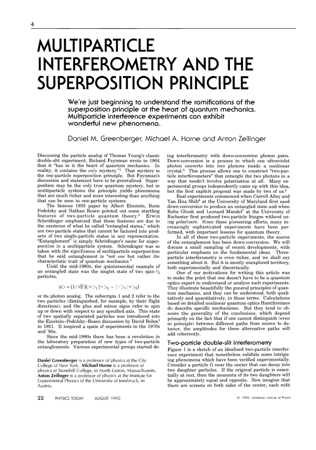
MULTIPARTICLE
INTERFEROMETRY AND THE
SUPERPOSITION PRINCIPLE
We're just beginning to understond the romificotions of the
superposition principle ot the heort of quontum mechonics.
Multiporticle interference experiments con exhibit
wonderful new phenomeno.
Daniel M. Greenberger, Michael A. Home and Anton Zeilinger
Discussing the particle analog of Thomas Young's classic
double-slit experiment, Richard Feynman wrote in 1964
that it "has in it the heart of quantum mechanics. In
reality, it contains the only mystery."^ That mystery is
the one-particle superposition principle. But Feynman's
discussion and statement have to be generalized.
Superposition may be the only true quantum mystery, but in
multiparticle systems the principle yields phenomena
that are much richer and more interesting than anything
that can be seen in one-particle systems.
The famous 1935 paper by Albert Einstein, Boris
Podolsky and Nathan Rosen pointed out some startling
features of two-particle quantum theory.^ Erwin
Schrodinger emphasized that these features are due to
the existence of what he called "entangled states," which
are two-particle states that cannot be factored into
products of two single-particle states in any representation.
"Entanglement" is simply Schrodinger's name for
superposition in a multiparticle system. Schrodinger was so
taken with the significance of multiparticle superposition
that he said entanglement is "not one but rather the
characteristic trait of quantum mechanics."
Until the mid-1980s, the quintessential example of
an entangled state was the singlet state of two spin-V2
particles,
|.^> = (l/V2")(|+X|->2 - |->i|+>2)
or its photon analog. The subscripts 1 and 2 refer to the
two particles (distinguished, for example, by their flight
directions), and the plus and minus signs refer to spin
up or down with respect to any specified axis. This state
of two spatially separated particles was introduced into
the Einstein-Podolsky-Rosen discussion by David Bohm^
in 1951. It inspired a spate of experiments in the 1970s
and '80s.
Since the mid-1980s there has been a revolution in
the laboratory preparation of new types of two-particle
entanglements. Various experimental groups started do-
Daniel Greenberger is a professor of physics at the City
College of New Yorl<. Michael Home is a professor of
physics at Stonehili College, in North Easton, Massachusetts.
Anton Zeilinger is a professor of physics at the Institute for
Experimental Physics of the University of lnnsbrucl<, in
Austria.
ing interferometry with down-conversion photon pairs.
Down-conversion is a process in which one ultraviolet
photon converts into two photons inside a nonlinear
crystal.^ This process allows one to construct
"two-particle interferometers" that entangle the two photons in a
way that needn't involve polarization at all. Many
experimental groups independently came up with this idea,
but the first explicit proposal was made by two of us.^
Real experiments commenced when Carroll Alley and
Yan Hua Shih^ at the University of Maryland first used
down-conversion to produce an entangled state and when
Ruba Ghosh and Leonard MandeF at the University of
Rochester first produced two-particle fringes without
using polarizers. Since these pioneering efforts, many
increasingly sophisticated experiments have been
performed, with important lessons for quantum theory.
In all of these two-particle experiments, the source
of the entanglement has been down-conversion. We will
discuss a small sampling of recent developments, with
particular emphasis on the fundamental ideas. Three-
particle interferometry is even richer, and we shall say
something about it. But it is mostly unexplored territory,
both experimentally and theoretically.
One of our motivations for writing this article was
to make the point that one doesn't have to be a quantum
optics expert to understand or analyze such experiments.
They illustrate beautifully the general principles of
quantum mechanics, and they can be understood, both
qualitatively and quantitatively, in those terms. Calculations
based on detailed nonlinear quantum optics Hamiltonians
do describe specific mechanisms. But they tend to
obscure the generality of the conclusions, which depend
primarily on the fact that if one cannot distinguish (even
in principle) between different paths from source to
detector, the amplitudes for these alternative paths will
add coherently.
Two-porticle double-slit interferometry
Figure 1 is a sketch of an idealized two-particle
interference experiment that nonetheless exhibits some
intriguing phenomena which have been verified experimentally.
Consider a particle O near the center that can decay into
two daughter particles. If the original particle is
essentially at rest, then the momenta of its two daughters will
be approximately equal and opposite. Now imagine that
there are screens on both sides of the center, each with
22
PHY5IC5 TODAY
AUGUST 1990
1990 Americon Insrirure of Physics
J
z
1
\^'
X. b'
^v ,
/a
ir
a >^
b\^
^
T
y
1
B
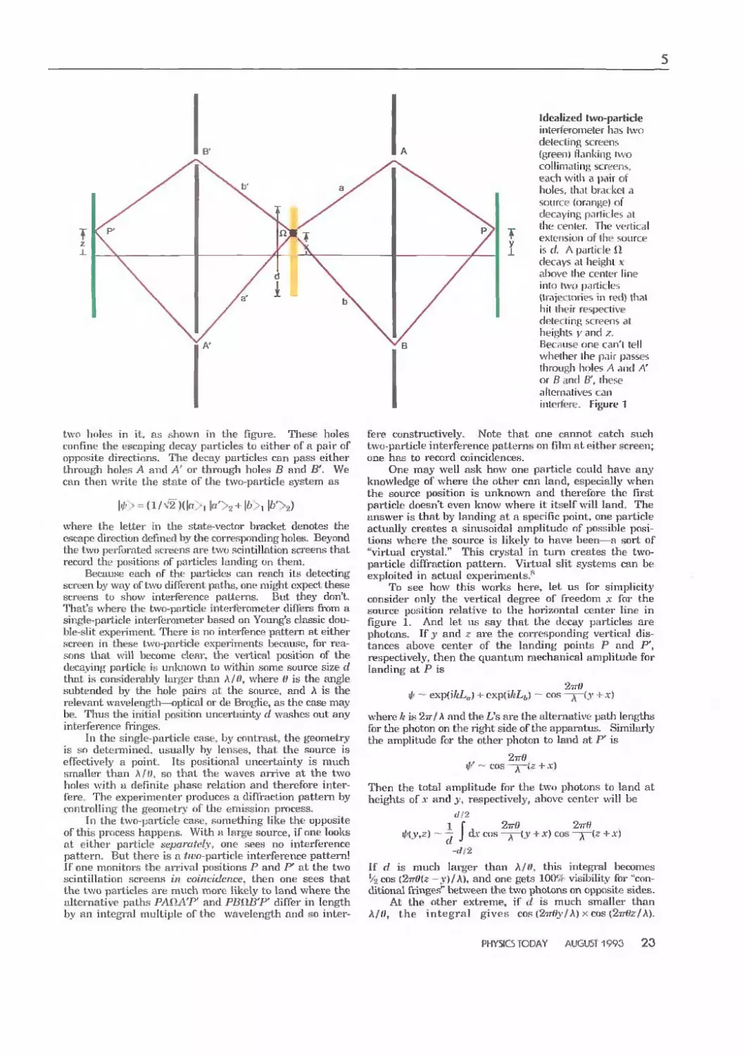
Idealized two-particle
interferometer has Ivvo
delecling screens
(green) flanking iwo
collimLi[inf> scrt'ens,
path with a ]wir ot
holes, thai biaclvci a
sniirte (orange) of
decaying pailicles at
the center. The vorlical
extension of ihp source
is d. A parlit le Xl
decays at height \
above the center line
into two prirlic'Ics
Orajoclories in red) that
hit their respective
delecting screens al
heights V and z.
Because one can't tell
whether ihe pair passes
through holes A Jtnd A'
or B and B', those
alternatives can
inlertere. Fijjure 1
two holes in it, fis shown in the figuie. Tliese holes
confine the escaping decay particles to either of a pair of
opposite directions. Tlie decay pailicles can pass either
through holes A and A' or through holes B and J5'. We
can then write the slate of the two-particle system as
y> > = (l/^^)(|ff;>, |n'>2+|6>, |6'>2)
where the letter in the state-\'ector bracket denotes the
escape direction defined by the corresi^onding holes. Beyond
the two perforated screens are two scintillation screens that
record the positions of particles landing on them.
Because each of the pailides can reacli ila detecting
screen by way of two difTei^cnt paths, one might exj^ecl these
ficreens to show intei-ference patlei'ns. But they don't.
That's where the two-particle interferometer difl'era from a
sinple-paii icie interferometer based on Young's classic
double-slit experiment. There is no interfence pattern at either
.screen in these two-particle experiments loecaiise, ft>r
reasons that will become clear, the vc;rlic£il i^osition of the
decaying particle is unluiown to witliin .some .source size d
that is considerdhly larger thaii A/f*, where 0 is the angle
subtended by the hole pail's at the source, and A is the
i-elevant wavelength—n])tical or de Bniglie, as the case may
be. Thus the initial po.sition uncertainty d washes out any
interference fringes.
In the single-particle case, by contrast, the geometry
is so detei-mined. usually by lenses, thai the source is
eflectively a point. Its positional uncertainty is much
smaller than A/H, so that the waves arrive at the two
holes with a definite phase relation and therefore
interfere. The experimenter produces a diffraction pattern by
controlling Ihe geometry of the emission pi*ocess.
In the Iwo-particle case, something like the opposite
of this process happens. With a large source, if one looks
at either particle separately, one sees no interference
pattern. But there is a ///'o-particle interference pattern!
If one monitors the arrival positions P and P' at the two
scintillation screens in coincidence^ then one sees that
the two particles are much more likely to land where the
alternative paths PAQAT' and PBilB'P' differ in length
by an integral multiple of the wavelength and so intei"-
fere constructively. Note that one cannot catch such
two-particle interference patterns on film at either screen;
one has to record coincidences.
One may well ask hnw one particle could have an^'
knowledge of where the other can land, especially when
the source position is unknown and therefore the first
particle doesn't even know where it itself will land. The
answer is that by landing at a specific point, one particle
actually creates a sinusoidal amplitude of po.ssible
positions where the source is likely to have been—a sort of
"virtual ciA'stal.*" This cry.stal in turn creates the two-
particle diffraction pattern. Virtual slit systems can be
exploited in actual experiments.^
To see how this works here, let us for simplicity
consider only the vertical degree of freedom x for the
source po.sition relative to the horizontal center line in
figure 1. And let us say that the decay particles are
photons. If y and z are the corresponding vertical
distances above center of the landing points P and P',
r-espectively, then the quantum mechanical amplitude for
landing at P is
?/' exp{iArL„) h- cxpti/^L/,) — cos —^y -i -v)
whei'C k is Stt/A and the i,\s are the alternative path lengths
for the photon on the right side of the apparatus. Similarly
tlie amplitude for the other photon to land at P' is
2frH
i}'* — cos ~j~l£ + X)
Then the total amplitude for the two photons to land at
heights of-Y and y, respectively, above center will be
1 f 2-jrO 27rW
i/r( >'.z) ~ — J dv cos -j;-{y + X) cos -;^U + x)
If d is much lai-ger than A/W, this integial becomes
'/a cos {27rOU -y)/A), and one gets lOO'/f visibility for
"conditional fringes" between the two photons on opposite sides.
At the other extreme, if d is much smaller than
A//^ the integral gives cos (27r«y/A) x cos {2Tr(iz/\).
PHY5IC5 TODAY AUGUST 1990 20
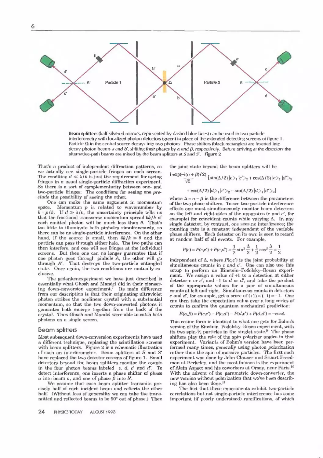
Beam splitters (half-silvered mirrors, represented by dashed blue lines) can be used in two-parlicle
interferomelry with localized photon detectors (green) in place of the extended detecting screens of figure I.
Particle il in the central source decays into two photons. Phase shifters (black rectangles) are insertoti into
decay-pholon beams .? and b'. shifting their pliases by a and p. respectively. Before arriving ar the detectors the
alternative-path beams are mixed by the beam splitters at 5 and S'. Figure 2
That's a product, of independent diflractioii patterns, so
we actually see sJnglG-particle fringes on each screen.
The condition d *^ X/d is just the requirement for seeing
fringes in a usual single-parliclo diffraction experiment.
So thei-e is u sort of complementarity between one- and
two-particle fringes: The conditions for seeing one pre-
cliide the possibility of seeing the other.
One can make the same argument in momentum
space. Momentum p is related to wavenumber by
k=p/ti. \f d ':^ XlO^ the uncertainty principle tells us
that the fractional transverse momentum spread bklk of
each emitted photon will be much less than 0. That's
too little to illuminate both pinholes simultaneously, so
there can be no single-pailicle intcrfei-ence. On the other
hand, if the source is small, then f>klk :» 0 and the
particle can pass through either hule. The two paths can
then interfere, and one will see fringes at the individual
screens. But then one can no longer guarantee that if
one photon goes through pinhole A, the other will go
through A. That destroys the two-jxirticle entangled
state. Once again, the two conditions are mutually
exclusive.
The gedankcnexperiment we have just described is
essentially what Ghosh and Mandel did in tlieir
pioneering down-conversion experiment.^ Its main difference
from our description is that their originating ultra\nolet
photon strikes the nonlinear crystal with a substantial
momentum, so that the two down-converted photons it
generates both emerge together from the hack of the
crystal. Thus Ghosh and Mandel were able to catch both
photons on a single screen.
Beam splitters
Most subsequent down-conversion experiments have used
a different technique, replacing the scintillation .screens
with beam splitters. Figure 2 is a schematic illustration
of such an interferometer. Beam splitters at S and S'
have replaced the two detector screens of figui'C 1. Small
detectors beyond the beam .splitters monitor the counts
in the four photon beams labeled c, d, c' and d'. To
detect interfeiHince, one inserts a phase shifter of phase
a. into beam a, and one of phase ^ into 6'.
We assume that each beam splitter transmits
precisely half of each incident beam and reflects the other
half. (Without loss of generality we can take the
transmitted and reflected beams to be 90'-' out of phase.) Then
the joint state beyond the beam splitters ^^^ll be
iexpH(o' + ^)/2)
V2-
|sin(A/2) |c>, |r'^o + cos(A/2) |c>, |t/'>2
+ cos(A/2) |f/>, |c'>2 - .sin(A/2) \dy^ |rf'>J
where A = a — /3 is the difference between the parametere
of the two phase shifters. To see two-particle interference
eilects one must, simultaneousl}' monitor beam detectors
on the letl and right, sides of the apparatus (c and c\ for
example) for coincident counts while varying A. In any
single detector, by contra.st, one sees no interference; the
counting rate is a constant independent of the variable
phase shifters. Each detector on its own is seen to record
at random half of all events. For example,
P(c) = P(c.c') + P{ii,d') = I sin-' - H I cos-' - = I
independent of A, where 'P{c,i:\ is the joint probability of
simultaneous counlii in e and c\ One can also use this
.setup to perform an Einstein—Podolsky—Rosen
experiment. We a.ssign a value of +1 to a detection at either
detector c or c', and -1 to d or d\ and take the product
of the appropriate values for a pair of simultaneous
counts at left and right. Simultaneous counts in detectors
c and d\ for example, get a score of (+1) x (—1) =-1. One
can then take the exp<jctation value over a long series of
counts to confirm the quantum mechanical prediction:
E{a,f3) = Picv) - Pied') - P(d^c') + P(dJ') = -cosA
This cosine form is identical to what one gets for Bohni's
version of the Einstein—Podolsky—Rosen experiment, with
its two spin-V'2 particles in the singlet state.^ The phase
shifters play the role of the spin polarizer angles in that
experiment. Variants of Bohm's version have been
performed many times, generally using photon polarization
rather than the spin of inas.sive particles. The fii*st such
experiment was done by John Clauser and Stuart Freed-
man at Berkeley, and the most famous is the experiment
of Alain Asi>ect and his coworkei-s at Oi-say, near Paris.'"
Witli the advent of the parametric down-converter, the
new version without polarization that weVe been
describing has also been done.'*
The fact that these experiments cxliibit two-particle
Correlations but not single-particle interference has some
important (if poorly understood) ramifications, of which
24
PHYSO TODAY AUGUST 1990
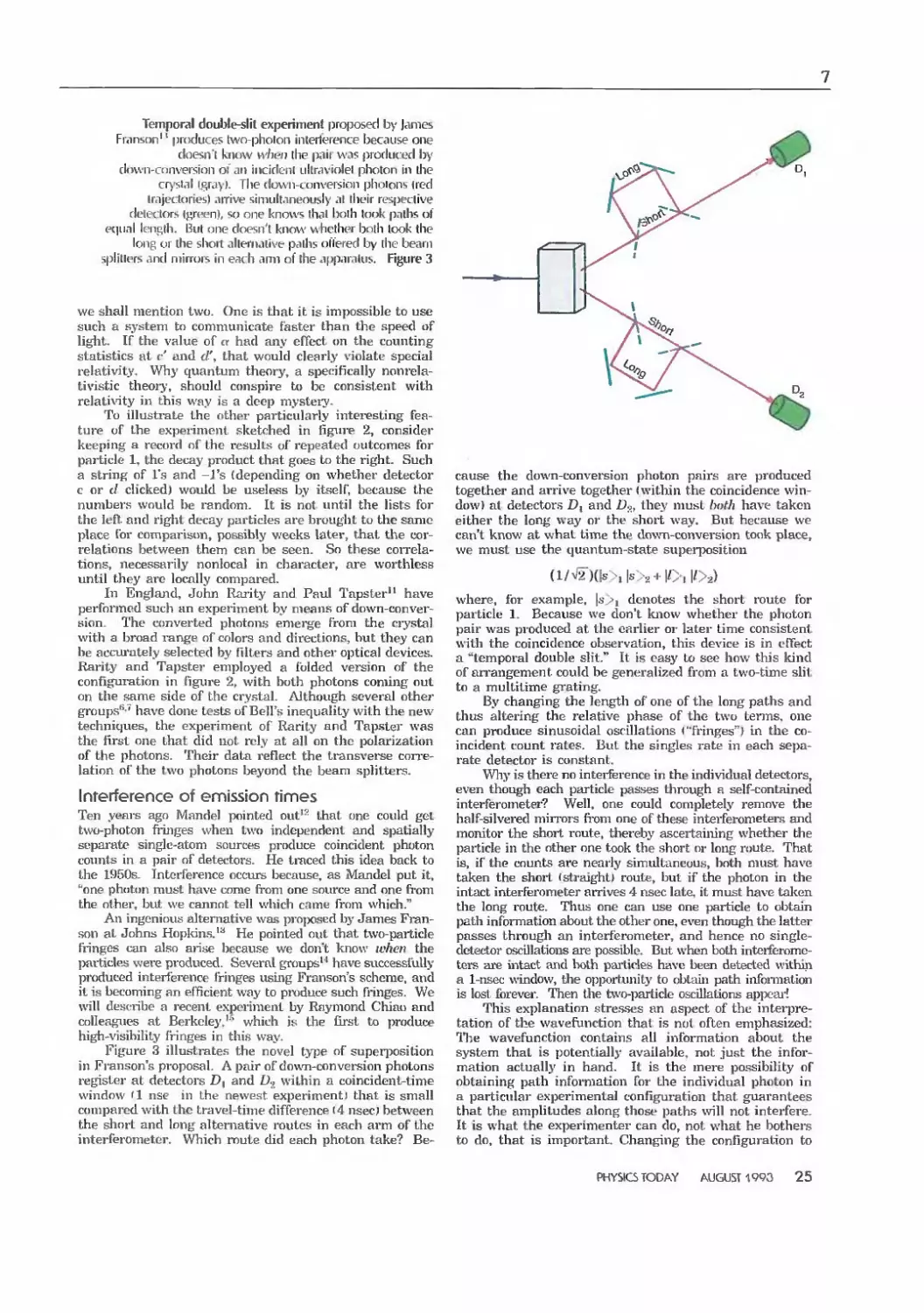
Temporal double-slit experiment pro|30sed by James
Fi.inson'' produces twn-photon intei1t?rente because one
doesn't know wln^n ihe paii was produced by
d^nvivccinveision oi\in iiicidcni ullraviolel photon in the
crystal igrayj. The down-tonversinn phnions tied
lraJL't.lt)iies) arrive simultaneously a! iheir resijocllve
detet tors (j^rcen), so one knows thai both tof)k paths ol
equal length. I?ut one doesn't know vshcther both look the
long or the shoil alternative paths offered by (he beam
splitlerN anri mirr(}i'; in each ami of the apparatus. Figure 3
WG shall mention two. One is ihat: if: is impossible to use
such a system tn communicate faster than the speed of
light. If the value of a had any effect on the counting
statistics at c' and d\ that would clearly violate special
relativity. Wliy quantum theory, a .specifically nonrela-
tivistic theory, should conspire to be consistent with
relati\nty in thi.s way is a deep mystei-y.
To illustrate the other pai"ticularly intei-esting
feature of the experiment sketched in fi^n-e 2, con.sider
keeping a record of the results of repeated outcomes for
particle 1, the decay product that goes to the right. Such
a string of l*.s and -J's (depending on whether detector
c or d clicked) would be useless by itself, because the
numbers would be random. It is not imtil the lists for
the lefl and right decay particles are brought to the same
place for comparison, possibly weeks later, tiiat the
correlations between them can be seen. So these
correlations, necessarily nonlocal in character, are worthless
until they are locally compared.
In Englajid. John l^*ity and Paul Tapster*' have
performed such an experiment by means of
down-conversion. The converted photons emerge from the crystal
with a broad range of colore and directions, hut they can
be accui'ately selected by fdters and other optical devices.
Rarity and Tapster employed a folded vei'sion of the
configuration in figure 2, with both photons coming out
on the same side of the cry.stal. Although several other
gi*oups''-^ have done tests of Bell's inequality with the new
techniques, the experiment of Rarity and Tap.ster was
the first one that did not rcly at all on the polarization
of the photons. Their data reflect the transverse cone-
lation of the two photons beyond the beam splittei^s.
Interference of emission times
Ten years ago Mandel ix)inted out''- that one could gel
two-photon fiijiges when two independent and spatially
separate single-atom sources produce coincident photon
counts in a pair of detectors. He traced this idea back to
the 1950s. Interference occurs because, as Mandel put it.
"one photon must have come from one source and one from
the other, but v\'e cannot tell which came fi'om v\hich."
An ingenious alternative was i^rojxJsed by James Fran-
son at Johns HopIdn.s.'^ He pointed out that two-paiticle
fringes can also aiise because we don't know when the
I)articlej3 were produced. Several gi*oups'' have successfully
I^roduced interference fringes using Franson's scheme, and
it is becoming an efficient way to pi^oduce such fringes. We
will describe a recent experiment by Raymond Chiao and
colleagues at Berkele}'.'* which is the fii'st to iM'oduce
high-visibility fringes in this way.
Figure 3 illustrates the novel t>^:e of superposition
in Franson's proposal. A pair of dowTi-conversion photons
register at detectors Z)| and O., within a coincident-time
window fl nse in the newest experiment) that is small
compared with the travel-time difference (4 nsec? between
the short and long alternative routes in each arm of the
interferometer. Wliich route did each photon take? Be-
D.
D.
cause the down-conversion photon pairs are produced
together and arrive together (within the coincidence
window) at detectors Di and D.j,, they must hoHi have taken
either the long way or the short way. But because we
can't know at what time the down-conversion took place,
we must use the quantum-state supenxisitioii
(l/v'2")(|s-,|s% + |/>,|/>2)
where, for example, |s>, denotes the short route for
particle 1. Because we don't Itnow whether the photon
pair was produced at the earlier or later time consisteni
with the coincidence observation, this device is in efTect
a "temporal double slit." It is easy to see how this Idiid
of an'angcment could be generalized from a two-time shI
to a multitime gi-ating.
By changing the length of one of the long paths and
thus altering the relative phase of the two tenns, one
can produce sinusoidal oscillations ("fringes"} in the
coincident count rates. But the singles rate in each
separate detector is constant.
Wliy is there no interference in the individual detectors,
even though each particle passes through a self-contained
interferometei*? Well, one could completely remove the
half-silvered mirroi-s fTOm one of the.se interferometers and
monitor the short route, tbei^eby ascertaining whether the
paiticle in the other one took the short or long route. That
is, if the counts are nearly simultaneous, both must have
taken the short (straight) route, but if the photon in the
intact interferometei* airives 4 nsec late, it must have taken
the long route. Thus one can use one particle to obtain
path information about the otlier one, even though the latter
passes through an intGrferometer, and hence no single-
detectoi' oscillations ai*e possible. But when both interfei-ome-
ters are intact and lioth pailicles have been detected withii^
a 1-nsec window, the opixntunit}' to obtain path infonnation
is lost forever. Then the two-i^article oscillations apix?aj*!
This explanation stresses an aspect of the
interpretation of the wavefunction that is not often emphasized:
The wavefunction contains all information about the
system that is potentially available, not ju.st the
information actually in hand. It is the mere possibility of
obtaining path information for the individual photon in
a particular experimental configuration that guarantees
that the amplitudes along those paths will not interfere.
It is what the experimenter can do, not what he bothers
to do, that is important. Changing the configuration to
PHYSICS TODAY AUGUST 1 WO 25
8
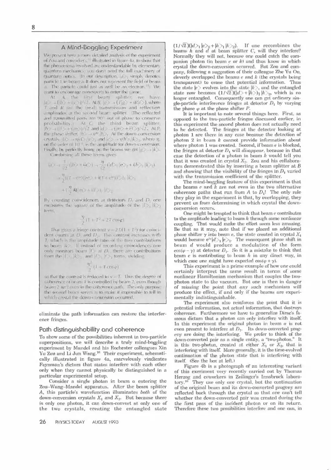
A Mind-Doggling Experiment
VV< pn*<j-"il 'ip""* I mi if^'-' (Icl.iil'f! .in.iK*-!'- oi ihp *"*\pi^*imenl
(if/(jii.mfKow itU'" ilhi-lMlP*'] in fipin tii u^ihou llwl
thf iiliPruviifHii iM\ i!v4^f'.irt iimVrsl.inH.iblplA clnmtMHiir^
r|uiiiitiitii I ti^rh.iiiK don I n-^ri llu' lull (iwi iiinpr\ (it
niiantui Dnlti (n «Mir (ios<'i|)lion MmpK deiiolt"
n.irlu |i 1 ir ln'.in .i ll H(»f« noi ifprcynllhu iVId fit luMrii
Th »*irhi li • iLikf iiisl .IS ".vpji hv .in '^k\ Iron Wf
mliii'^ni lUMiit'niinpxjvr*' t<» renter ilu u-im*
\* i *hi' biM'" pfiM ■ w'f hti\p
(' MW -(i ^iKi/ ) uhen-
ill N th( H,i| r.insmis-^iiiii rinrl rplJet lion
.impltiurlc^^ I ]Ii '(iinil Iif.im sphllrr. Tin* retlnrtcfj
(iiiti [rjiisniillc'fl piiils .iro '[> tjut oi ph.ist in c nnsor\-i>
probabditv * lh<^ third bi ^ln splutf-r
h • .inrl i^y in -»-1./ » J. A( P
/h( fli.js -,. /*/"• " '■ \I \\jo lU^vn-^onvo'won
r\-,l,iK ' . 171. tind f ► >;'// A whfu- jj
on t' <fHi^i I r ''ii- .impliliiilo inr dovvn-i onvrr<,rnn.
linnlK U\ pprln tK linirn; i>[ ibf bi-jm-. wo tlcl k .
( ni>ii>i iini till lhf'».i »rrns ive-
111
' rr
»;
i(T
riff
^i\h
^.Ri
f^- . ouMiini
!TII .Wll'^'^ 11II
tCfT
rhcii "=■
dfni Miinl
7 hif»
'<iii\ I If mil ji
iiniidomp'. <il dHo« Inr^ D .ind n onf
^iliMi wi II1H .iniphhidi Oi thi '
nn V i * mlr.i ■!»-_! f 1
cinti D T'li'- 1 lUilrHM
I tut tOMK I
rIM ^ Witll
■nplihulr iiro fir h two r ontribiilinn*.
i«.(»Mrl nl •'( (jivhn ( oiiif idt'ni,( nn^'
iru' '"^ » •■»■'• \H'Uiin
1li(ii ibc iiniT isi K r(^iLri.i^rl lo T Ihu^ Ihi fI^^^O(. 01
uhrn-'ni it iif.in I !»• i'inlroll<:i*< i)\ Iv.iiii * t'xi'ii llnuit'b
i}t\m 'sn I in (lie 1 ithvrau 1* pjffi Jhr on\\ pwrpr*-.
Ihr <;i^rorid \m\\\ i '^•i lo m.ikf il impKssihlf lo tfll in
^ -v-si.il l!if dowiiH »nv<>rsion O'' urifd.
eliminate tho path information can ivstore the
interference fringes.
Path distinguishobility and coherence
To show some oi the possibiHties inhevpnt in two-particle
superpositions, we will describe a truly mind-boggling
experiment by Mandel and his Rochester colleagues Xin
Yu Zou and Li Jun Wang.'*^ Their experiment,
schematically illustrated in figure 4a, marvelously vindicates
Feynman's dictum that states iuteribre with each otiier
only when they cannot physically be distinguished in a
particular experimental setup.
Consider a single photon in beam a entering the
Zou-Wang-Mandel apparatus. Mter the beam splitter
A. this particle's wavefunction illuminates both uf llie
down-conversion crystals X^ and X.3. But because ihei*e
is only one photon, it can down-convert at only one of
the two crystals, creating the entangled state
(l/V2)(|t/>i |e>.2 + |A ">! lA-'^n). If one recombines the
bpams h and d at beam splitter C, will tliey interfere?
NoiTnally t]ie>' will not. bpcause one could catch the com-
paniun photon (in b«nn e or k) and thun luicjw in which
crystal the down-con version f>ccurrcd. Bui Zou and
company, following a suggestion of their colleague Zhe Yu Ou,
cleverly overlapped tlie beajns e and A> (the crystals being
transparent) to erase that potential information. Thus
the state |e^ evolves into the state |/(- *. and the entangled
state now becomes (l/>/2)(|c/ ' + |// Oi K' '2» ^vhicli is no
longer entangled. Consequently one cun get ordinai-y
single-particle interference fringes at dctucUir Di by vaiying
the phase ip at the phase shifter P.
It is important to note several things here. First, as
opposed to the two-particle fringes discussed earlier, in
this experiment the second photon does not actually need
lo he detected. The fringes al the detector looking at
photon 1 are there in any case because the detection of
photon 2 in beam k cannot provide information aboiil
wheie photon 1 was created. Second, if beam e is blocked,
the fringes at detector D, will diauppcar, because in that
case the detection of a photon in beam k would tell you
that it was created in crystal X.^. Zou and his
collaborators demonstrated this by inserting a beam splitter at B
and showing thai the \'isibility of the fringes in i), varied
with the transmission cneOicient of the splitter.
The mind-boggling featui-e of this expeiiment is that
the beams c and k ai-e not even in the two alternative
coherence paths that run from A to D^. The only role
they play in the experiment is that, by overlapping, they
prevent us from determining in which ciystal the down-
conversion oceur.s.
One might be l^mpted to think tliat be;ui\ c contributes
to the amplitude leading to beam h through some nonlinear
coupling. That would make the ellect seem less amazing.
Be that as it may, note that ii' we placed an additional
phase shifter y into beam e, the state created in cry.stal A'^i
would become e'^|r7 , |tV2. The consequent phase shift in
beam d would produce a modulation of the form
costv? - y) at detector D^. .So it is a nuVitake to think that
beam e is contributing to beam // in any direct way, in
wliich case one might have expectt^d cosicp+ y).
This experiment is a prime example of how one could
certainly interpret the same residt in terms of .some
nonlinear Hamiltonian mechanism that couples the two-
photon state to the Vdcuum, But one is then in danger
of miasiiig the point that any .such mechanism will
produce the effect, if and only if the beams are
experimentally indistinguishable.
The experiment also reJnJbives the point that it is
potential information, not actual information, that destroys
coherence. Fiulhermore we have to generalize Dirac's
famous dictum that a pholxm can only inteifere with itself.
In this experiment the original photon in beam a is not
even present to interiere at Dy lis down-tonverted
progeny are doing thp interiering. We pi'efer to think of the
down-converted pair as a single entity, a "two-photon." It
is this two-photon, created al either X\ or X'2, that is
interfering with itself More generally, it i.s the time-evolved
continuation of Ihe photon state that is interfering with
itself (See the box at left.)
Figure 4b is a photograph of an interesting variant
of this exeriment very recently carried out by Thomas
Herzog and coworkers in Zeiliiiger's Innsbruck
laboratory."* They use only one crystal, jjut the continuation
of the original beam and its down-converted progeny are
reflected back through the crystal so that one can't tell
whether the down-con verted pair was created during the
the first pass of the incident photon or on its return.
Therefore these two possibilities interfere and one can. in
26
Pi-IYSICS TODAY AUGUST 1990
a
■V
T^
effpcL, enhance or sup- XX^
pivss Lhe atomic eniission ^ **
process in the crystal by
small movomenU of" mii'-
roi*s til at are several feet
dway! . -■'.•
The quonrum eraser '////:
Figiii'c 5 .shows an
experimental arrangement first ' *' '
used by Alley and Siiih,*'
and recently expluitud by
Paul Kwiat and coworkers
at Berkeley'' to demon-
strate Marian Snilly's no- ; ^'
tion of a "ciiuintuni eraser."
Others have called it
"haunted" or "phantom"
measurement.'*^ To
appreciate the basic idea.
fh:st suppose that only the
i>eam splitter is in the path
of the two beams emei^s'ns '
from Uie down-con vertei*
ci-yslal. This arrangement
produces an interesting
and very basic two-particle
effect: Both particles must end up in tiie same detector.''*
The reason is simple. To get coincident counts at the
two detectors, either particle 1 (the photon that ultimately
lands in detector 1) takes route a and paj-ticle 2 ttikes i-oute
h, or vicf versa. In the former alt.ernative, both photons
are reflected by the beam splitter, each reflection
contributing a 90' phase shift to the overall amplitude. The latter
alternative, by contrast, involves nn phase-shifting
reflections. TliUK the twi» alternative amplitudes aic 180*^ out of
phase with each other, and they cancel.
So if both beams are, for example, horizontally
polarized, Lhey will remain so, and there will be no
coincident counts in detectors I and 2. But if we now inserl
a 90' polarization rotator into beam ft, it will become
vertically polarized and the two amplitudes will no longer
interfere because one can tell which path a photon took
to its detector by measuring its polarization. Thus there
Hi
\:\\
t
•A-
- ' *. *. \ '. *. * • "• *. *. •.
, : : -. ; : \ \'. •• *. •, •. -
• : : *. -. • • *. '- •■
■>» . -
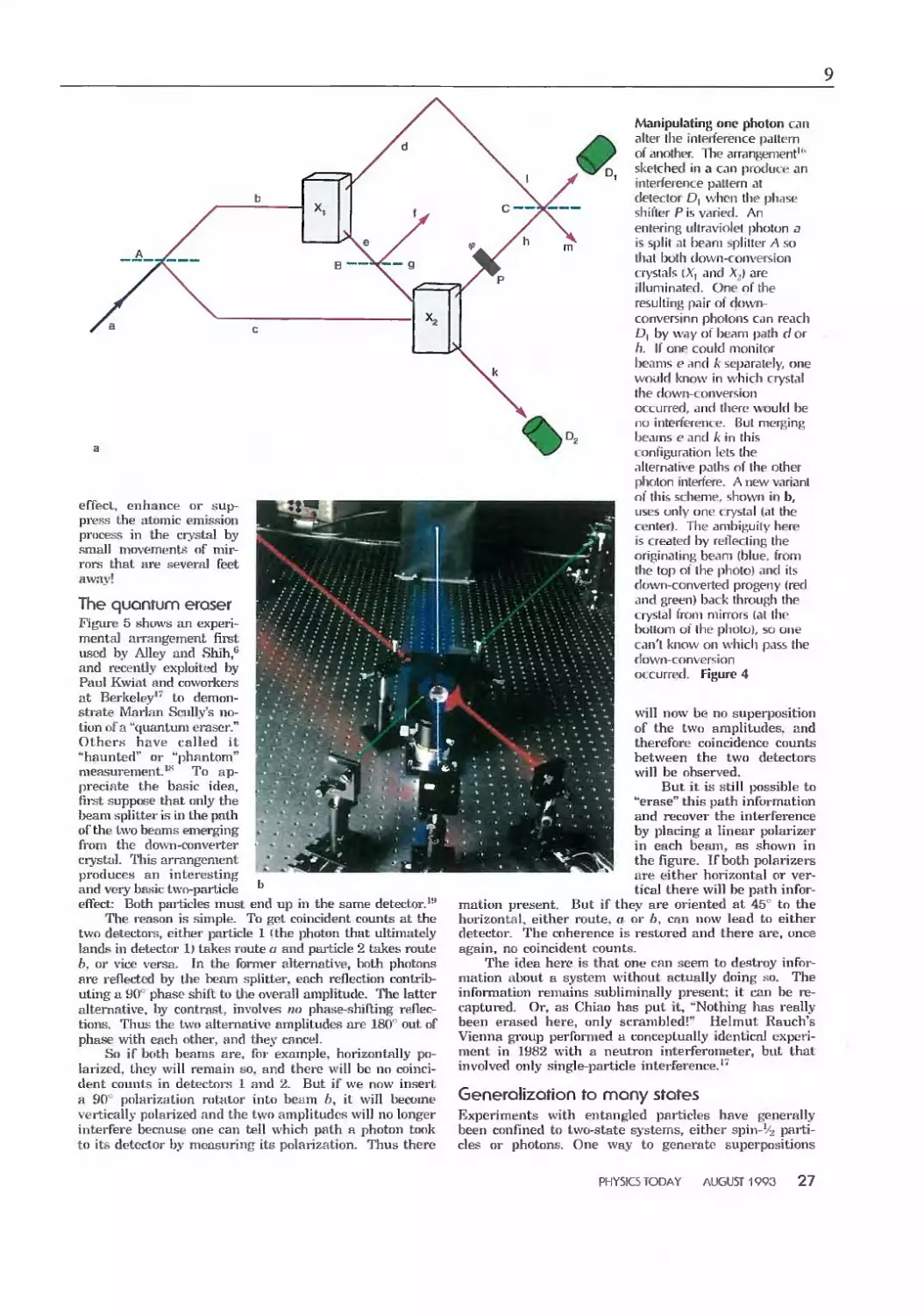
Manipulating one photon ci\n
alter IJie inlPifereiice paltern
of anolhtT. 1 he arrangement'"
D sketched in a can produce an
interference pallein a!
delecloi D, when the phase
shifter P Is varied. An
enlering ullrdviolol photon o
is split dt bedm spliller A .so
that both clown-conversion
crystals (X, and X.) are
illuminated. One of the
resulting pair of dovvn-
conversinn photons can reach
/J| by way of beam path c/or
h. If one could monitor
beams e rind k separately, one
would know in which cr>'stal
the down-conversion
occurred, and there would be
no interference. But merging
beams e and k in this
lontiguration U'ts the
alternative paths of the other
photon interfere. A new variant
of this schemc>, shown in b,
uses only one c rystal (at the
center). The ambiguity here
T is created by reflecting the
originating beam (blue, from
the top of the photo) and its
dfAvn-converted progeny (red
and green) back through the
crystal from mirrors (at tho
bottom of the plioto), so one
can't know on which pass the
down-convei sion
occurred. Figure 4
4
r
»
s
will now be no superposition
of the two amplitudes, and
therefore coincidence counts
between the two detectors
will be observed.
But it is still possible to
"erase" tliis path information
and i-ecover the interference
by placing a linear polarizer
in each beam, as shown in
the figure. If both polarizers
are either horizontal or
vertical there will be path
information present. But if they are oriented at 45"" to the
horizontal, either route, a or h, can now lead to either
detector. The coherence is restored and there are, once
again, no coincident counts.
The idea here is that one can seem to destroy
information about a system without actually doing so. The
information remains subliminally present: it can be
recaptured. Or, as Chiao has put it, "Nothing has really
been erased here, only scrambled!" Helmut Ranch's
Vienna group performed a conceptually identical
experiment in 1982 with a neutron interferometer, but that
involved only single-particle interference.''
GenerolizQtion to mony states
Experiments with entangled particles have generally
been confined to two-state systems, either spin-V^
particles or photons. One way to generate superpositions
PhtYSiCS TODAY AUGUST 1990 27
10
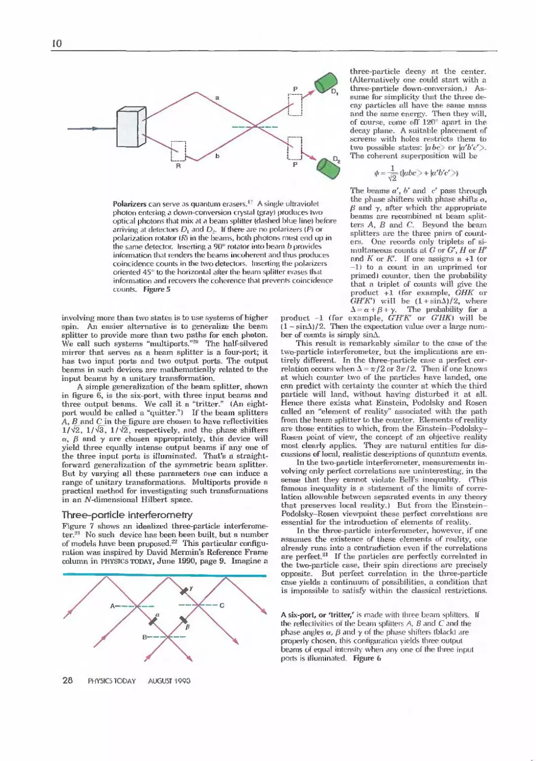
Polarizers can serve as quantum erasers.' A sinj^k* ultraviolet
photon entering J down-conversion ciystal (pray) produces two
optical photons ihat mix at a beam splitter (clashed blue line) belore
arrivinj^ at deteLtois D| and O.. It there are mi polarizers (P) or
polari/alion rolalor iR\ in the beams, both photons must lmicI up in
the same detector. Inserting a 90* rotator into beam b provides
information that renders the beams incoherent and thus produces
coincidence counts in the two detectors. Inserting; (he polarizers
oriented 45'' to the horizontal after the beam splitter erases that
infonnalion unci recovers the coherence that prevents coincidence
counts. Figure 5
involving more than two states is to use systems of higher
spin. An easier alternative is to generalize the beam
splitter to pi-ovide more than two paths for each photon.
We call such systems "tnultiports."-" The half-silvered
mirror that serves as a heam splitter is a four-port; it
has two input ports and two output ports. The output
beams in such dc\qcps are mathematically related to the
input beams by a unitiiry transfbi-mation.
A simple generalization of the beam splitter, shown
in figure 6, is the six-port, with three input beams and
three output beams. We call it a "tritter." (An eight-
port would be called a "quitter.") If the beam splitters
Ay ^and C in thetigure are chosen to have reflectivities
1/V2, 1/V3^, l/"^2, respectively, and the phase shifters
/3 and y are chosen appropriately, this device will
product 1 ffor
a
yield three equally intense output beams if any one of
tlie three input ports is iHuminated. That's a
straightforward generalixation of the symmetric beam splitter.
But by varying all these parameters one can induce a
range of ujiitary transformations. Multiports provide a
practical method for investigating such transformations
in an iV-dimensional llilbert space.
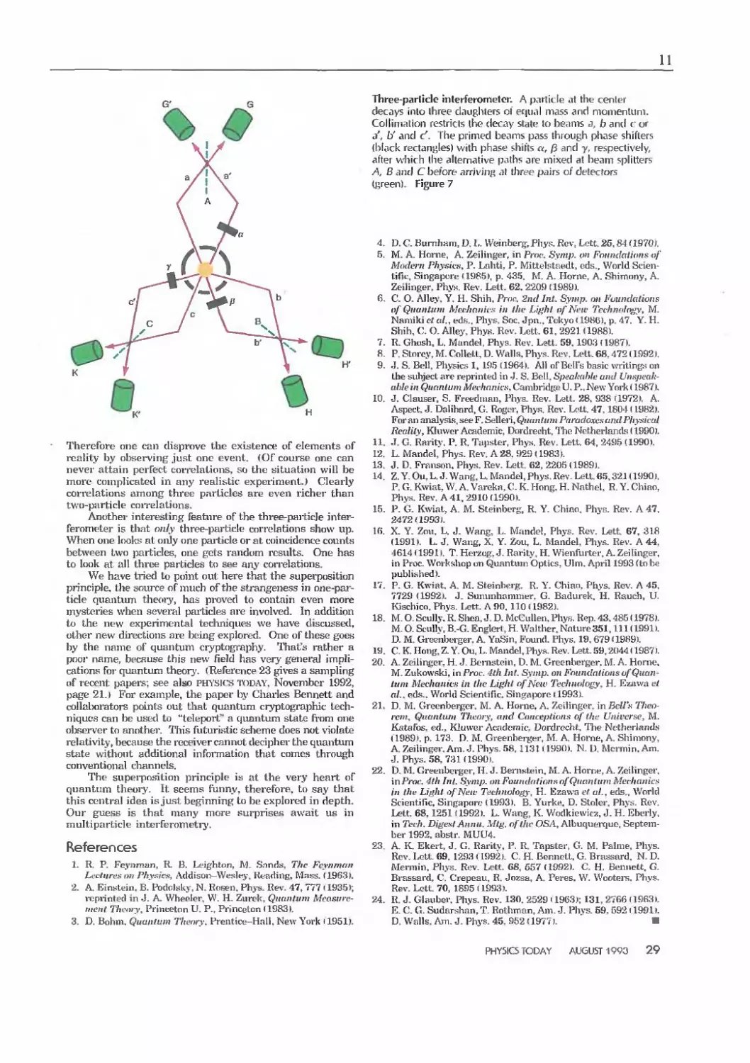
Three-portJcle Interferometry
Figure 7 shows an idealized thiee-particle
interferometer.--' No such device has been been built, but a number
of models have been proposed.^^ Tliis particular
configuration was inspired by David Mermin's Reference Frame
column in PHYSICS TODAY, June 1990, page 9. Imagine a
three-particle decay at the center.
(Alternatively one could start with a
Q thi-ee-particle down-conversion.)
Assume for simplicity that the three
decay particles all have the same mass
and the same enei-gy. Then they will,
of cour.se. como off 120' apai-l in the
decay plane. A suitable placement of
screens witli holes restricts llieni to
two possible states: \cthc or |o7/t'>.
Q The coherent superposition will be
The beams a\ h' and c pass through
the phase .shillcra with phase shifts a,
jtf and y, after which the appropriate
beams ai'e recombined at beam spht-
ters A, B and C. Beyond the beam
splitters arc the three paii-s of
counters. One records only triplets of si-
Tnultaneous counts at G or G\ II or //'
and K or IC. If one assigns a +] (or
-IJ to a count in an unpnmed <or
primed) counter, then the probability
that a triplet of counts will give tlic
product +1 (for example, GHK or
GIVK') will be fl + sinA)/2, whei-e
A = « + /3 I y. The probability for a
example, G'H'K or G'UK) will be
(1 - sinA)/2. Then the expectation value over a lai'ge
number of counts is simply sinA.
This result is remarkably .similar to the case of the
two-particle interferometer, but the implications are
entirely different. In the thi-ee-particle case a jierfect
correlation occiu's when A = 7r/2 or 37r/2. Then if one knows
at wliich counter Iavo of the particles have landed, one
can predict with certainty the counter at which the third
particle will land, v^ithout having disturbed it at all.
Hence thei-e exists what Einstein, Podolsky and Rosen
called an ''element of reality" associated with the path
from the heam splitter to the counter. Elements of reality
are those entities to which, fi-om the Einstein-Podolsky-
Rotsen point of view, the concept of an objective reality
most clearly applies. They are natural entities for
discussions of local, realistic descriptions of quantum events.
In the two-particle interferometer, measui'ements
involving only perfect correlations ai-e unintei'esting, in the
sense that they cannot violate Bell's inequality. (This
famous inequality is a statement of the limits of
correlation allowable between separated events in any theoiy
that preserves local reality.) But from the Einstein—
Podolsky—Rosen viewpoint these perfect coirelations are
essential for the introduction of elements of reality.
In the three-particle intei-ferometcr, however, if one
assumes the existence of tliese elements of reality, one
already runs into a contradiction even if the coiTelations
are perfect.'^' If tlie particles are perfectly correlated in
the two-particle case, their spin directions are precisely
opposite. But perfect correlation in the three-particle
case yields a continuum of possibilities, a condition that
is impossible to satisfy within the classical restrictions.
A six-port, or 'trilter/ is maile wilh lliree beam splitters.
the rerleclivities ot the beam splilters A, B and CanrI the
phase angles «, fi and y of the phase shifter*, (blackj are
properly chosen, this conti^uralion yields three output
beams of equal intenslly when any one of the three input
|X)rts is illuminated. Figure 6
28
PhtYSICS TODAY AUGUST 1990
11
G'
K
H'
K'
H
Therefore one can disprove the exiistence of elements of
i-ealily by observing just one event. (Of course one can
never attain perfect con'ehttions, so the situation will be
more complicated in any realistic expeiiment.) Clearly
correlations among three particles ai-e even richer than
two-particle coirelations.
Anothei- intei^esling featui'e of the three-particJe intei--
ferometer is that only three-particle correlations show up.
When one looks at only one paiticle or at coincidence counts
between two paiticles, one gets random results. One has
to look at all three particles tf) see any correlations.
We have tried to point out here that the superposition
principle, the souire of much of the strangeness in
one-particle quantum theoi^, has pi-oved to contain even more
mysteries when several paiticles are involved. In addition
to the new experimental teclmiques we have discussed,
other new dii*ections are being explored. One of these goes
by the name of quantum cryptogi-aphy. That's rather a
poor name, because this new field has very general
implications for quantum theory'. (Reference 23 gives a sampling
of recent papers; see also Ptn'sics 'IV)DAY, November 1992,
page 21.) For example, the paper by Charles Bennett and
collaborators points out that quantum cryptographic
techniques can be used to "teleport" a Cjunntum state fi-om one
observer tf) another. This futuristic scheme does not violate
relativity, because the i-eceiver cannot deciphei- tlie quantum
state without additional information that comes through
conventional channels.
The superpo.sition principle is at the very heart of
quantum theory. It seems funny, therefore, to say that
this central idea is just beginning to be explored in depth.
Our guess is that many more surprises await us in
multiparticle interferometrj'.
References
1. R. P. Feynman, R B. Leighton, J\']. .Snnd.s, The Feyninan
Li'ctitivs nti Physics, Addison-Wesley. Reading. Mass. (1963).
2. A. EiriKtein. B. Podol.sky. N. Rosen, Phys. Rev. 47, 777 (1935);
i-opvintecl in J. A. Wheeler. W. H, Zurck. Qitantmn
Measurement Theory, Princeton U. P., Princeton (1983).
3. D. Bohm. Quantum Theory. Prentice-Hall. New York < 1951).
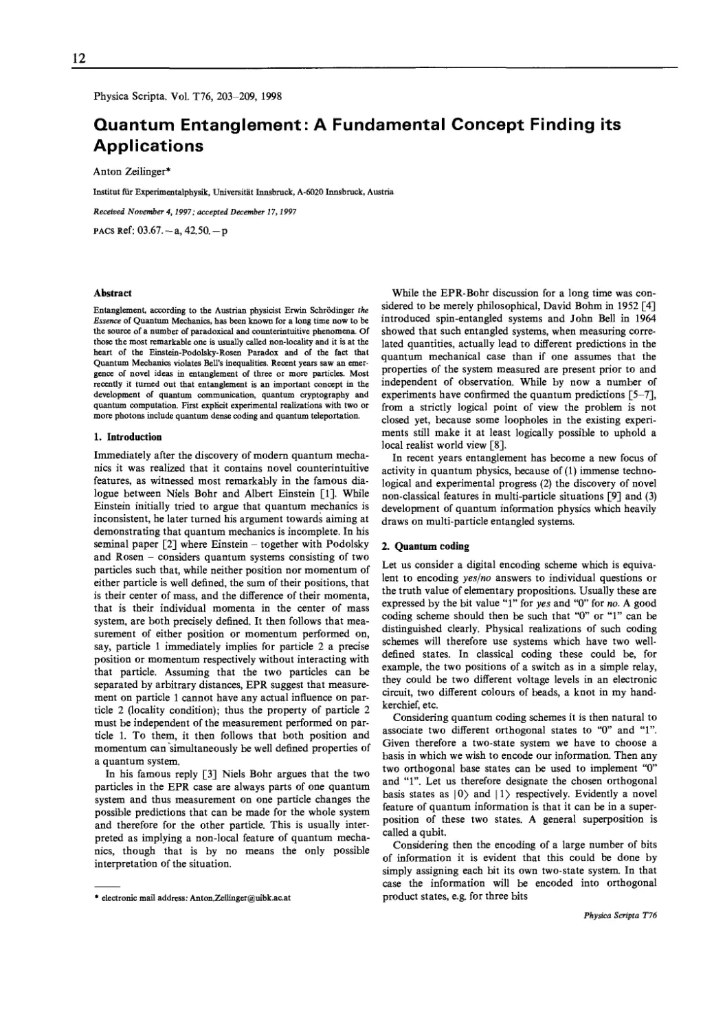
Three-parlicio interferometer. A particle *it the center
deciiys inlo Ihree daughters ot er|u.il mass and niomenluni.
Collinirilion restricts the decay state to beams j, h and r oi
a', b' and c'. The primed beam*, pass through phase shifters
(black rectangles) with phase shifts a, fi and y, respectively,
after which (he alternative paths are mixed at beam splitters
A, B dJid C before arrivin/^ al ibrer pairs of detectors
(j^reen). Figure 7
5.
6.
7.
8.
9.
10.
11.
12.
13.
14.
15.
Ui.
17.
18.
IH.
20.
21.
22.
23.
24.
D. C. Bumhani, D. L. Weinberg, Fliys. Rev, Lett. 25,84 (1B70;.
M. A. Hoine, A. Zeilinger, in Pmc. Symp. on Foundationa of
Modern Physics, P. Lnhti, P. Mittelstaedt, eds.. World Scien-
tifii:. Singapcrt- I1S)85). p. 435. M. A. Home, A. Shimcmv, A.
Zeilinger, Phy.-^. Rev. Lett. 62.2209 (1989).
C. O. Alley. Y. H. Shih. Proc. 2nd Int. Symp. on Foundations
of Quantum Mcrhnnivs in the Liftht of New Technology, M.
Namiki ct al., eds.. Phys. Soc, Jpn.. Tckyo (198C). p. 47. Y. H.
Shih. C. O. Alley, Ph.v«. Rev. I^tt. 61, 2921 (19881.
R- Ghcsh. L. Mandel. Phys. Rev. Lett. 59.1903 (1987).
P. Storey, M. Colletl, D. Walls. Phys. Rev. Lett. 68,472 (1992).
J. S. Bell. Plivsics 1. 195 (1964k All nf Bell's basic writings on
the subject are reprinted in J. S. Bell. Sjyeahahle and
Unspeakable in Qnnntum Mechanics, CambridETP U. P., New York (1987).
J. Clauser, S. Freedinan. Phvs. Rev. Lett. 28. S)38 il972K A.
Aspect. J. Dalihnrd. G. RogLM\ Phyp. Rev, Lott. 47,1804 (1982).
For fin ana]ysi.s. see F. Seller!, Quantum Paradoxes and Physical
Reality, Kkuver Academic, Dnrdrecht, The Net herlanda (1990),
J. G. Rarity. P. R. Tap-ster, Phy.s. Rev. Lett. 64. 2495 (1990).
L. Mandel, Phys. Rev. A 28. 929 (19831.
J. D. Franson. Phys. Rev. Lett. 62, 2205 (1989).
Z. Y. Oil, L. J. Wang. L. Mandel, Phys. Rev. LetL 65,321 (19901.
P. G. Kwiat. W. A. Vareka, C. K. Hong. H. Nnthel. R. Y. Chino,
Phys. Rev. A 41, 2910 (1990 k
P. G. KwiaU A. M. Steinberg, R. Y. Chino. Phys. Rev. A 47.
2472aSS3j.
X. Y. Zou. L. J. Wang. L. Mandel, Ph^-s. Rev. Lett. 67, 318
(1991k L. J. Wang, X. Y. Zou, L. Mandel, Phy.s. Rev. A 44,
1614 i 19911. T. Herzog, J. Rarity. 11. Wienfurter. A. Zeilinger.
in Proc. Workshop on Quantum Optics, Ulm. April 1993 (to be
published).
P. G. Kwiat. A. M. Steinberg. R. Y. Chinn, Phys. Rev, A 45.
7729 (1992). J. Sumnihamnier. G. Badurek. 11. Rauch. U.
KJschico. Phys. Lett. A DO. 110 (1982).
M. O. Scully. R. Sliea. J. D. McCuUen. Phys. Rep. 43.485 (1978).
M.O. Scully,B.-G. Englerl,H. WalLher.Nature351. Ill (1991).
D. M. Greenbeiger. A. YnSin, Found. Phys. 19.679 (1989).
C. K. Hong. Z. Y. Ou, L. Mandel, Phys. Rev. Lett. 59.2044 (1987).
A. Zeilinger. H. J. Bernstein, D. M. Greenberger. M. A. Home,
M. Zukowski, in Proc. 1th Int. Symp. on Foundations of
Quantum Mechanics in the Lij^ht of New Technology, H. E-zavva et
al.. pds.. World Scienlific. Singapore [ 1993).
D. M. Greenberger. M. A. Ilorne. A. Zeilinger. in Bcirs Thco-
ivni. Quantum Theory, and Conceptions of the Unircrsej M.
Katafbs. ed., Kluwer Academic. Dordrecht. The Ntrthrrl.incls
(1989 k p. 173, 0. M. Greenberger, M. A. Home. A. Shimony,
A. Zeilinger. Am. J. Phys. 58.1131 \ 1990k N. I). Mermin. Am.
J. Phys. 58. 731 f 1990 k
D, M. Greenberger, H. J. Bern.sk'in. M. A. Horne, A. Zeilinger.
inPmr. 4th Int. Symp. on Foundations nf Quantum Mechanics
in the Light of New Technology, H. lilzawa et al.. eds.. World
Scientiric. Sing-npore (1993). B. Yurkt\ D. Sloler. Phys. Rev.
Lett. 68.1251 (1992k L. Wang, K. Wodkiewicz, J. H. Ebi-rly,
in Tech. Digest Annu. Mtg. of the OSA, AlbuqueiYjuo,
September 1992. abstr. MULI4.
A. K. Ekert. J. G. Raritv, P. R. Tapster, G. M. Palme, Phys.
Rev. I^tt. 69. 1293 (lS)92k C. R BonnctL. G. Brassard. N. D.
Mermin. Phys. Rev. Lett. G8, 557 (19.92). C. H. Bennett, G.
Brassard, C. Crepeau, R. Jozsa, A. Peres. W. Wootere. Phys.
Rev. Lett. 70, 1895 1 l9S)ak
R. J. Glauber. Phys. Rev. 130. 2529 il963.i; 131, 2766 (tn63k
E. C. G. Sudarshan, T. Rothman, Am. J. Phvs. 59. 59211991 k
D. Walls. Am. J. Phys. 45. 952 (1977). ■
PHYSICS TODAY AUGUST 1990 29
12
Physica Scripta. Vol. T76, 203-209, 1998
Quantum Entanglement: A Fundamental Concept Finding its
Applications
Anton Zeilinger*
Institut fur Experimentalphysik, Universitat Innsbruck, A-6020 Innsbruck, Austria
Received November 4,1997; accepted December 17,1997
PACs Ref: 03.67. - a, 42.50. - p
Abstract
Entanglement, according to the Austrian physicist Erwin Schrodinger the
Essence of Quantum Mechanics, has been known for a long time now to be
the source of a number of paradoxical and coimterintuitive phenomena. Of
those the most remarkable one is usually called non-locahty and it is at the
heart of the Einstein-Podolsky-Rosen Paradox and of the fact that
Quantum Mechanics violates Bell's inequalities. Recent years saw an
emergence of novel ideas in entanglement of three or more particles. Most
recently it turned out that entanglement is an important concept in the
development of quantum commimication, quantum cryptography and
quantum computation. First exphcit experimental realizations with two or
more photons include quantum dense coding and quantum teleportation.
1. Introduction
Immediately after the discovery of modem quantum
mechanics it was realized that it contains novel counterintuitive
features, as witnessed most remarkably in the famous
dialogue between Niels Bohr and Albert Einstein [1]. While
Einstein initially tried to argue that quantum mechanics is
inconsistent, he later turned his argument towards aiming at
demonstrating that quantum mechanics is incomplete. In his
seminal paper [2] where Einstein - together with Podolsky
and Rosen - considers quantum systems consisting of two
particles such that, while neither position nor momentum of
either particle is well defined, the sum of their positions, that
is their center of mass, and the difference of their momenta,
that is their individual momenta in the center of mass
system, are both precisely defined. It then follows that
measurement of either position or momentum performed on,
say, particle 1 immediately impHes for particle 2 a precise
position or momentum respectively without interacting with
that particle. Assuming that the two particles can be
separated by arbitrary distances, EPR suggest that
measurement on particle 1 cannot have any actual influence on
particle 2 (locaHty condition); thus the property of particle 2
must be independent of the measurement performed on
particle 1. To them, it then follows that both position and
momentum can simultaneously be well defined properties of
a quantum system.
In his famous reply [3] Niels Bohr argues that the two
particles in the EPR case are always parts of one quantum
system and thus measurement on one particle changes the
possible predictions that can be made for the whole system
and therefore for the other particle. This is usually
interpreted as implying a non-local feature of quantum
mechanics, though that is by no means the only possible
interpretation of the situation.
electronic mail address: Anton.Zeilinger@uibk.ac.at
While the EPR-Bohr discussion for a long time was
considered to be merely philosophical, David Bohm in 1952 [4]
introduced spin-entangled systems and John Bell in 1964
showed that such entangled systems, when measuring
correlated quantities, actually lead to different predictions in the
quantum mechanical case than if one assumes that the
properties of the system measured are present prior to and
independent of observation. While by now a number of
experiments have confirmed the quantum predictions [5-7],
from a strictly logical point of view the problem is not
closed yet, because some loopholes in the existing
experiments still make it at least logically possible to uphold a
local reahst world view [8].
In recent years entanglement has become a new focus of
activity in quantum physics, because of (1) immense
technological and experimental progress (2) the discovery of novel
non-classical features in multi-particle situations [9] and (3)
development of quantum information physics which heavily
draws on multi-particle entangled systems.
2. Quantum coding
Let us consider a digital encoding scheme which is
equivalent to encoding yes/no answers to individual questions or
the truth value of elementary propositions. Usually these are
expressed by the bit value "1" for yes and "0" for no. A good
coding scheme should then be such that "0" or "1" can be
distinguished clearly. Physical realizations of such coding
schemes will therefore use systems which have two well-
defined states. In classical coding these could be, for
example, the two positions of a switch as in a simple relay,
they could be two different voltage levels in an electronic
circuit, two different colours of beads, a knot in my
handkerchief, etc.
Considering quantum coding schemes it is then natural to
associate two different orthogonal states to "0" and "1".
Given therefore a two-state system we have to choose a
basis in which we wish to encode our information. Then any
two orthogonal base states can be used to implement "0"
and "1". Let us therefore designate the chosen orthogonal
basis states as |0> and 11> respectively. Evidently a novel
feature of quantum information is that it can be in a
superposition of these two states. A general superposition is
called a qubit.
Considering then the encoding of a large number of bits
of information it is evident that this could be done by
simply assigning each bit its own two-state system. In that
case the information will be encoded into orthogonal
product states, e.g. for three bits
Physica Scripta T76
13
204 A. Zeilinger
|0>|0>|0>
|0>|0>|1>
|0>|1>|1>
|1>|0>|0>
|1>|1>|0>
ll>ll>ll>.
(1)
The corresponding, in general 2", states form a complete
orthonormal basis for the n-qubit space. Yet, alternatively,
in such a space we could also choose very different bases
which even could be entangled. A maximally entangled basis
for two independent particles, two qubits, is
|f'+> = 4=(|0>il> + |l>|0».
'P'>^4=(i0>|l>-|l>|0»,
<P+> = 4=(|0>|0> + |1>|1»,
<P'> = 4=(|0>|0>-|1>|1».
(2)
This is the so-called Bell basis. It is important to notice
that here we can still encode two bits of information, that is
we have four different possibiUties, but now this encoding is
done in such a way that none of the bits carries any well-
defined information on its own. All information is encoded
into relational properties of the two qubits. It thus follows
immediately that in order to read out the information one
has to have access to both qubits. The corresponding
measurement is called a Bell-state measurement. This is to be
compared with the classical case where access to one qubit
is simply enough to determine the answer to one yes/no
question. In contrast, in the case of the maximally entangled
basis access to an individual qubit does not provide any
information.
3. Quantum communication and dense coding
Whenever, say, two parties A (AHce) and B (Bob) wish to
communicate with each other they have to agree first on a
coding procedure, that is they have to agree which symbol
means what. In classical coding the situation is very simple.
Restricting ourselves to binary information, that is to bits,
we need some information carrier which has two states. A
famous historic example from the American revolution was
when Paul Revere informed the Revolutionaries about the
path taken by the Royals by displaying one or two lamps in
the steeple of Old North Church in Boston. In quantum
physics again we can have information encoding in a novel
way using entangled states and thus encode information
into joint properties of elementary systems. Then the
elementary systems themselves do not carry any information.
A first elementary case where this is clearly demonstrated is
quantum dense coding.
The maximally entangled Bell basis of eq. (2) has a very
important and interesting property which was exploited by
Bennett and Wiesner [10] in their proposal for quantum
2 bit
Bell-state
coding
Bell-state
measurement
2 bit
ALICE
Fig. 1. In quantum dense coding Bob, having access to one of the two
entangled qubits only, can actually encode two bits of information, because
he can switdi aroimd in the full Bell basis. Ahce can identify the
information encoded by performing a complete Bell-state measurement on the
entangled pair.
dense coding. This is the property that in order to switch
from any one of the four Bell states to all other four it is
sufficient to manipulate only one of the two qubits while in
the classical case one has to manipulate both. Thus, the
sender Bob (Fig. 1) can actually encode two bits of
information into the whole entangled system by just manipulating
one of the two qubits. Let us, for example, assume that we
start from the state | !f ^> then we can obtain | If ^> by just
introducing a phase shift of n onto, say, the second qubit,
|^^> is obtained by flipping the second qubit and the last
state I ^^ > is obtained by a combination of both.
In order to read out this information the receiver, Ahce,
needs to be able to identify the four Bell states, that is she
needs a Bell-state analyzer. It can be shown that, in order to
identify all four Bell states, one needs some non-hnear
interaction between the two qubits. In our experimental
realization [11] of the dense coding scheme it was possible by just
using hnear elements like beam splitters and polarizers to
identify three of the four possibihties and thus to encode
and identify log2 3 = 1,58 bits of information per photon
manipulated.
4. Photon statistics at a beam splitter and Bell-state analysis
Formally speaking Bell-state analysis is not a problem. All
you have to do is project any incoming state onto the Bell
basis and you will find out by repeating the experiment
with which probabihty the original state can be found in
one of the Bell states. The experimental problem is that thus
far no complete Bell-state analyser exists in the laboratory
for any kind of quantum systems. This is due to the fact that
complete Bell-state analysis requires non-hnear interaction
between the two qubits [12] which has not been realized so
far.
Interestingly, partial Bell-state analysis is possible
exploiting the statistics of two qubits at a beam sphtter. The basic
principle of that Bell-state analyser rests on the observation
that of the states in equation 2 one state is antisymmetric.
This is the | If ^> state which clearly changes sign upon
exchange between the two particles. The other three states
are symmetric. We thus observe that the qubit obeys fer-
mionic symmetry in the case of | If ^> and bosonic
symmetry in case of the other three states. Thus far we have not
identified whether we use bosons or fermions in our
experimental scheme. In fact, the four Bell states could very well
Physica Saipta T76
14
Quantum Entanglements 205
be either those of fermions or those of bosons. This is
because the states written in equation 2 are not the
complete states but can be amended by a spatial state which
also could be symmetric or antisymmetric. Then, in the case
of bosons the spatial part of the wave function has to be
antisymmetric also for the !f ^ state and symmetric for the
other three, while for fermions this has to be just reverse.
Let us first consider two photons, cleariy bosons, where
we assume that the Bell states above describe the
polarization of the photons, that is, an internal degree of freedom.
Then, cleariy, the total state of the two photons has to be
symmetric. For the case of the two particles incident
symmetrically onto a beam spHtter (Fig. 2), one from each mode
I a> and 16>, the possible external states are
^A> =
^S> =
1
a>|6>-|6>|a».
ay\by + \by\ay).
(3)
where | !f ^> and | !f s> are anti-symmetric or symmetric
respectively. Because of the requirement of symmetry the
total two-photon states are
\^^>\^s>- (4)
We note that only the state anti-symmetric in external
variables is also anti-symmetric in internal variables. It is
this state which also emerges from the beam splitter in an
external anti-symmetric state. This can easily be found by
assuming firstly that the beam spHtter does not influence the
internal state and secondly that at the beam spHtter we have
a phase shift of n/2 upon reflection. Actually it can easily be
seen [13] that the spatially anti-symmetric state is an eigen-
state to any beam spHtter operator. In contrast, in all three
cases of the symmetric external state | If s> the two photons
emerge together in one of the two outputs of the beam
spHtter. This behaviour of symmetric states can readily be
demonstrated even using photons in an unentangled
internal state [14]. Figure 3 and 4 show the consequent
experimental behaviour [15] for the entangled internal state | If ^>
and that for the internally antisymmetric state | If ^ >.
It is therefore evident that the state | If ^> can clearly be
discriminated from all the other states. It is the only one of
the four Bell states which leads to coincidences between
Fig. 2. A beam splitter with two inputs a and b and two outputs c and d.
We assume that two particles are incident onto the beam splitter one from
each side. The particles can then arise in two ways one in each of the two
output ports, they are either both reflected or both transmitted. For
bosonic states these two possibilities interfere destructively while for fer-
mionic states they interfere constructively.
10000
7500-
5000-
2500-
O
c
•73
• I—I
O
c
.1—1
o
-1,0 -0,5 0,0 0,5 1,0
Flight Time Difference x (ps)
Fig. 3. Coincidence coimts behind a beam spHtter as a function of the
difference of arrival time of two photons in an internally symmetric entangled
state. For large time differences the two photons are distinguishable and
therefore they behave independently and a certain coincidence rate equal to
the classical rate is observed. For zero time difference there are no
coincidences because both photons always leave the beam spUtter together in
the same output port.
detectors placed on each side after a beam spHtter. How can
we then identify the other three states? It turns out that
distinction between | If ^> on the one hand and |^^> and
I ^^> on the other hand can be based on the fact that only
in I If ^> the two photons have different polarization while
in the other two they have the same polarization. Thus
performing polarization measurements and observing the
photons on the same side of the beam sphtter one can
determine whether they are in the state | If ^> or in one of the
states I ^^> and | ^^>. It should be remarked that a
generalization of this procedure impHes that any three orthogonal
maximally entangled states can be distinguished from each
other in the same way, because by local unitary
transformations one can perform rotations in the two-dimensional
Hilbert-space.
Consider now the same experiment with fermions where
again the Bell states describe the internal states, for example
if the two qubits are entangled in spin. We then find that
10000
7500-
5000-
2500-
O
c
•73
• I—I
O
c
.1—1
o
-1,0 -0,5 0,0 0,5 1,0
Flight Time Difference x (ps)
Fig. 4. Coincidence rate for two photons in the internally antisymmetric
entangled state. Here again for large time differences we obtain the classical
behaviour. When the time difference approadies zero we get twice the
coincidence rate implying that the two photons never leave the beam sphtter
together in the same output port.
Physica Scripta T76
206 A. Zeilinger
15
the four possible states now are
(5)
because of the antisymmetry requirement of the total state.
For fermions therefore only one of the states is spatially
symmetric, the other three are spatially anti-symmetric. It
will thus be in only one of the cases, namely for | !f ^> that
both fermions will emerge together from the beam spHtter.
In all other three cases they will emerge from different sides
[16]. Yet, remarkably, it is again this state which can
immediately be distinguished from the other three because of its
distinct symmetry properties.
5. Entanglement swapping and the nature of quantum
information
Entanglement used to be considered as a consequence of the
fact that the entangled particles interacted in their past or
that they came from a common source. That this is too
restricted a view is witnessed by the concept of
entanglement swapping [17]. In the simplest case of entanglement
swapping we take two entangled pairs (Fig. 5) and subject
two particles, one from each source, to a Bell-state
measurement. Then the other two particles which have never
interacted in the past and also did not come from a common
source are projected into an entangled state.
This experiment, whose realization is presently proceeding
in Innsbruck [31], has some deep impHcations for the
meaning of information in quantum physics. As mentioned
above, entanglement between two quantum systems impHes
that at least some information is stored only in joint or
relational properties of the two systems. In the case of maximal
entanglement there is actually no information stored in any
individual particle, all information is carried by all the
particles jointly. This fact in itself poses already a challenge for
a naive reahst position. How can it be that particles have
well-defined joint properties - for example when we know
that their polarizations in a certain basis are equal -
without carrying any properties by themselves? For a Bell
state each of the systems is completely unpolarized on its
Bell-state
measurement
-PBS
^BellX
Source)
\iy
>
XSeTK
[Source
\ny
>
own? In the case of entanglement swapping this interpretive
problem is even more striking.
Let us, for simpHcity of discussion, just consider the case
where we have sources that produce our two qubits in the
anti-symmetric state | !f ^>. This state has the unique feature
that it is anti-symmetric in any basis. Thus, in terms of its
information content, the statement is that we know the two
qubits are different whatever basis we choose^. We thus
know simply by the choice of preparation that in each of the
two entangled pairs to be used in entanglement swapping
the two qubits are completely different.
We now have to discuss the information content of Bell-
state analysis. At first we note that, whichever states we
would produce at the sources, a fair Bell-state analyser will
return any of the four possible answers with equal
probability of 25%. That is, the action of the Bell-state analyser is
such that it projects the two photons onto an entangled
state and, since in our case the two qubits are themselves
members of maximally entangled pairs and therefore carry
no information, this has to happen with equal probabifity
for all four Bell states measured. In fact, the Bell-state
measurement does not reveal any information about any of the
qubits emitted by one of the two sources nor any joint
information about each source. Yet, what we gain is joint (or
relative) information about the two sources.
Suppose, specifically, that in a certain experimental run
we obtain the result | !f^> for the Bell-state measurement.
We then know that qubits 2 and 3 have been projected by
the measurement onto a state which is characterized by the
fact that these two qubits are different in whatever basis.
Interestingly, and again most remarkably, this statement is
even true as none of the two qubits themselves are yet well-
defined in any basis and have no properties by themselves.
Now we are in a position to complete our chain of
reasoning. By the properties of source 1 we know that qubit
1 and qubit 2 are different. By the result of the specific Bell-
state measurement we know that qubit 2 and 3 are different
and, finally, from the property of source 2 we know that
qubit 3 and 4 are different. Therefore, since our qubits are
defined in a Hilbert-space of dimension 2 only, we conclude
that qubits 1 and 4 also have to be different in any basis.
Therefore they emerge in the anti-symmetric state | !f ^>.
Analogous reasoning can be built up for the other three
possible Bell-state measurement results.
This analysis supports the interpretation that quantum
mechanics is just a formulation of what can be said about
quantum systems very much in the spirit of Bohr [18]. The
question as to what "really" the properties of these quantum
systems are is empty and devoid of any meaning.
We could go even one step further realising that in
quantum physics information has a novel quafity which
goes beyond its nature in classical physics. In classical
physics it is natural to assume that the objects we observe
Fig. 5. In entanglement swapping two Bell sources I and II emit one pair
of entangled qubits eadi. One then performs a Bell-state measurement on a
pair consisting of one qubit from each source. This projects the two
outermost qubits which have never interacted onto an entangled state.
^ We remark that for the three symmetric states we can make analogous
statements but the situation is sUghtly more comphcated. It turns out in
the end that, since the Hilbert-space of the four Bell-states is four-
dimensional, we can encode two independent bits of information into
these four states. Therefore the four states can be characterised by yes/no
answers to two distinct questions. These two questions are questions
about the identity of the two qubits in two different bases conjugate to
each other.
Physica Scrtpta T76
16
exist prior to and independent of any measurement and the
information we gain by measurement is an entity of
secondary quality while the objects are primary. In contrast it is
suggestive that in quantum physics the situation is that
information can be a primary quality and the objects with
their properties have a secondary quaUty, they can be
constructed in retrospect after the information has been gained
in a measurement. This is consistent with Bohr's Caveat
that we should be very cautious about making mental
pictures of quantum systems. Such pictures are only allowed in
the context of a specific experimental setup. In fact, most of
the misunderstandings and misinterpretations of quantum
mechanics result from assuming that quantum objects have
properties prior to and independent of the specific
apparatus chosen to observe them.
6. Quantum teleportation and the non-locality of information
A most remarkable appHcation of the concept of
entanglement is quantum teleportation. Consider first the problem.
Suppose that AHce has an object which Bob, who could be
anywhere, might need at a certain time. In classical physics
what she can do is perform many precise measurements on
the object and send the information to Bob who then can
reconstitute the object. Within classical physics the accuracy
of this is only limited by the precision with which Alice can
measure and by the technical abifities of Bob. Yet, we know
that in the end any measurement will run into the
limitations imposed by quantum mechanics. It is evident that
no measurement whatsoever performed by Alice can reveal
the full quantum state of the object. We therefore ask which
strategy can Alice pursue in order for Bob to obtain the
object in its full quantum state when he needs it.
A strategy proposed by Bennett et al. [19] uses exactly the
information-theoretic features of entanglement mentioned
above. According to that protocol, AHce and Bob have to
share in advance an entangled pair of quantum states (Fig.
6). Let us consider for simpHcity that the object is simply a
two-state system, a qubit. Then AHce and Bob share from
the beginning an ancillary entangled pair which for
convenience we again consider to be in the state | If^).
Subsequently AHce performs a Bell-state measurement on her
qubit and one of the two ancillaries. As discussed above, for
BOB
Unitary
Operation
^
^
2 bit
Bell-state
measurement
ALICE
Fig. 6. In quantum teleportation AHce performs a joint Bell-state
measurement on her initial particle and on one of an entangled ancillary pair from
the Bell source. This then projects the other particle of the ancillary into a
state which Bob can bring into exactly the original state of the initial
particle using one of the four imitary transformations according to Ahce's Bell-
state measurement result.
Quantum Entanglements 207
the case of entanglement swapping, AHce will obtain each
one of the four possible answers with equal probabifity, that
is her original qubit and her qubit from the ancillary pair
will be projected onto any one of the four Bell-states each
with probabihty 25%. We note again that this measurement
does not reveal any information, neither about the
properties of the original qubit nor about the properties of the
ancillary pair. So AHce obtains one of four possible results,
"¥'+", "f'^", "^+", or "^^". She then broadcasts this
information, that is two classical bits, such that Bob can receive
them. By now Bob is in posssession of a specific state as a
consequence of Alice's Bell-state measurement. Performing
one of four unitary transformations depending on Afice's
specific result Bob can transform his particle into the
original qubit. We also note that the original qubit disappears
during the Bell-state measurement, it looses its identity, and
thus Bob's qubit is not a copy but really a teleported
reappearance of the original.
A remarkable property of the scheme is that the four
unitary operations Bob has to perform are completely
unrelated to the state AHce wants to teleport. This is because
Ahce's Bell-state measurement does not convey any
information about the original state.
The experiment can most easily be understood again on
the basis of the fact that the meaning of entanglement is that
it represents relational statements between quantum
systems. So, in the case of teleportation we have to use
entanglement twice, firstly when the ancillary pair is
produced and secondly in the Bell-state measurement. It thus turns
out that the entanglement of the ancillary pair imphes a
well-defined relation between these two qubits without
defining their individual properties, and the Bell-state
measurement imphes a well-defined relation between the qubit
to be teleported and one of the ancillaries. Therefore, the
second ancillary, by the same chain of reasoning as above in
our discussion of entanglement swapping, is in a well-
defined relationship to the original qubits to be teleported.
It is again this remarkable feature of information in
quantum mechanics that we have a closed chain of logical
reasoning about relational properties without any statement
on the properties of the individual systems.
The major problem in the experimental verification of
quantum teleportation [20] is the Bell-state measurement of
two independently created quantum systems. This means
that these two qubits have to be measured such that their
identity is lost, that it is not possible to infer which detection
event refers to which source. It turns out that in the
experiment it is rather tricky to achieve this situation. As can be
seen in [21], it involves an elaborate application of a
quantum erasure technique.
7. Multi-qubit entanglement in quantum computation
The most complex apphcation of quantum entanglement
discussed presently is quantum computation [22]. Quantum
computation heavily uses superposition of multi-qubit
systems, i.e. entanglement. Therefore it is natural that
among the most basic paradigms in the field are the
production and analysis both of Bell states and of so-called
GHZ states [23], i.e. three-qubit entanglements.
From the point of view of the novel possibihties
introduced by quantum computation it is important to realize
Physica Scripta T76
17
208 A. Zeilinger
that superposition of multi-qubit states makes massive
quantum parallelism possible [24]. This is that fact that a
quantum computer can produce the result of various
different inputs at the same time if the input state is a
superposition of the individual informations. Consider, for
example, that using standard binary encoding the most
simple GHZ state can be interpreted as a superposition of
two numbers
1
(1000> + 1111> = 4- (I "0"> + I "7"»
(6)
that is, it represents a superposition of the numbers "0" and
"7". Taking this as the input to a Hnear quantum computer
it will produce in the output a superposition of the results
corresponding to the two inputs.
It is well known that a most important practical problem
a future quantum computer faces is decoherence due to
coupling to the environment. Somewhat analogous to
classical computers decoherence can be viewed as a quantum
analogue of classical noise and it can be overcome using
redundant information. Therefore, quantum error correction
codes [25] utilize the possibihty of encoding n qubit into the
states of a Hilbert-space of higher dimension N. One then
exploits the additional degrees of freedom to ehminate the
quantum noise. This, naturally, implies entangled qubits in a
Hilbert-space of high dimension.
While the field of quantum computation is signified
presently by development of a vast number of different codes
and theoretical approaches, the status of experiments is to
verify the individual elementary steps including two-qubit
quantum gates. It is presently completely open whether
future development will utilize multi-photon states as
discussed in this paper, quantum encoding into individual
atoms [26] or individual ions [27] in trap configurations or
bulk nuclear magnetic resonance techniques [28]. Yet, the
fundamental individual steps in all these techniques are all
the same from a quantum information science point of view.
8. Concluding comments
There are several further applications of entanglement in
information science. One of them is the use of EPR pairs in
quantum cryptography as proposed by Ekert [29]. There
one actually uses a test of Bell's inequahty to find out
whether or not an eavesdropper has gained any access to
the qubits sent.
Another concept utihzing entanglement is quantum
computation in distributed networks [30]. This concept
presently is in the stage of ideas and has not yet found experimental
verification. It would imply extensive use of quantum tele-
portation, of Bell-state measurements, of entanglement
swapping, and of multi-particle entanglements.
Taken together, all the examples given above demonstrate
already now that quantum entanglement is one of the most
important novel concepts in information science. It is
furthermore not unreasonable to even expect future
applications of entanglement in information technology itself. This
is supported by the observation that the present
development of information technology towards further and
further miniturization will reach the single quantum limit
sometime in the first decades of the next century. Once that
happens information technology will by necessity be
quantum. The radically new features of quantum
entanglement let us expect that this will not just be a limitation but
that it will open up completely novel possibihties for
communication and computation.
The intricate interpretive questions raised by the multiple
use of entanglement in the examples given here and as
discussed above underline once more the deep conceptual
problems of quantum reahty. It is hard to beheve that there
is a possibility to escape Niels Bohr's verdict "There is no
quantum world, there is only an abstract quantum
description".
Acknowledgements
The author thanks the Nobel Committee for its hospitality. This work was
supported by the Austrian Science Foundation (FWF), project S65/04 and
by the US National Science Foundation (NSF), grant number PHY97-
22614. I also wish to acknowledge the collaboration with all members of
my group at the University of Innsbruck.
References
1. Bohr, N., "Discussions with Einstein on Epistemological Problems in
Atomic Physics" in Albert Einstein: Philosopher-Scientist" (Edited by
P. A. Schilpp) (The Library of Living Philosophers, Evanston 1949), p.
200.
2. Einstein, A., Podolsky, B., and Rosen, N., Phys. Rev. 47, 777 (1935).
3. Bohr N., Phys. Rev. 48, 696 (1935).
4. Bohm, D., "Quantum Theory" (Prentice-Hall, Englewood Chffs. NJ,
1951) p. 614.
5. Freedman, S. J. and Clauser, J. S., Phys. Rev. Lett. 28, 938-941 (1972).
6. Aspect, A., Grangier, P. and Roger, G., Phys. Rev. Lett. 47,460 (1981);
49, 91 (1982); Aspect, A., Dalibard, J. and Roger, G., ibid. 49, 1804
(1982).
7. Kwiat, P. G, et al. Phys. Rev. Lett. 75,4337 (1995).
8. Pearle, P. M., Phys. Rev. D2,1418 (1970); Clauser, J. F. and Shimony,
A., Rep. Prog. Phys. 41,1881 (1978).
9. Greenberger, D., Home, M. A. and Zeilinger, A., "Bell's Theorem,
Quantum Theory, and Conceptions of the Universe", (Edited by M.
Kafatos) (Kluwer, Dordrecht, 1989) p. 69; Greenberger, D. M., Home,
M. A., Shimony, A. and Zeilinger, A., Amer. J. Phys. 58,1131 (1990).
10. Bennett, C. H. and Wiesner, S. J., Phys. Rev. Lett. 69, 2881 (1992).
11. Mattle, K., Weinfurter, H., Kwiat, P. G. and Zeihnger, A., Phys. Rev.
Lett. 76,4656 (1996).
12. Michael Reck, impublished.
13. Zeilinger, A., Bernstein, H. J. and Home, M. A., J. Modem Opt. 41,
2375 (1994).
14. Hong, C. K., Ou, Z. Y. and Mandel, L., Phys. Rev. Lett. 59, 2044
(1987).
15. Oberparleiter, M., Diploma-thesis, University of Innsbruck, 1997,
impubhshed.
16. Loudon, R., "Coherence and Quantum Optics VI" (Edited by J. H.
Eberly and L. Mandel) (New York: Plenum, 1990), p. 703; Loudon,
R., "Disorder and Condensed Matter Physics" (Edited by J. A. Black-
man and J. Taguena) (Oxford: Qarendon, 1991), p. 441.
17. Zukowski, M., Zeilinger, A., Home, M. A. and Ekert, A. K., Phys.
Rev. Lett. 71,4287 (1993).
18. Nagel, B., in "Possible Worlds in Humanities, Arts and Sciences".
(Proceedings of Nobel Symposium 65) (Edited by Sture Allen)
(Gruyter, Berlin 1989), p. 388.
19. Bennett, C. H. et al, Phys. Rev. Lett. 70, 1895 (1993).
20. Bouwmeester, D. et al., Experimental Quantum Teleportation, Nature
390, 575 (1997).
21. Zukowski, M., Zeilinger, A. and Weinfurter, H., "Fimdamental
Problems in Quantum Theory" (Edited by D. M. Greenberger, A.
Zeilinger) (Annals of the New York Academy of Sciences, 1995) vol.
755, p. 91.
Physica Scripta T76
18
Quantum Entanglements 209
22.
23.
24.
25.
26.
C. H. Bennett, Phys. Today 48,24 (1995).
Brass, D., Ekert, A., Huelga, S. F., Pan, J.-W. and Zeilinger, A., Phil.
Trans. R. Soc. Lond. A (1997) in press.
Shot, P. W., in Proc. of the 35th Ann. Symp. on the Foundations of
Computer Science, Los Alamitos, CA, (IEEE Press, New York 1994);
Ekert, A., Jozsa, R., Rev. Mod. Phys. 68,733 (1996).
Shot, P. W., Phys. Rev. A52, 2493 (1995); Steane, A. M., Proc. Roy.
Soc. Lond. A452,2551 (1996).
Hagley, E. et al, Phys. Rev. 79,1, (1997).
27. Monroe, C. et d., Phys. Rev. Lett. 75, 4714, (1995); Wineland, D., this
volume.
28. Gershenfeld, N. A. and Chuang, I. L., Science 275,350 (1997).
29. Ekert, A. K., Phys. Rev. Lett. 67,661 (1991).
30. Cirac, I., Zoller, P., Kimble, J. and Mabuchi, H., Phys. Rev. Lett. 78,
3221 (1997); Bose, S., Vedral, V. and Knight, P. L., Phys. Rev. A57,
822 (1998).
31. Pan, J.-W., Bouwmeester, D., Weinfurter, H. and Zeilinger, A., Phys.
Rev. Lett. 80,3891 (1998).
Physica Scripta T76
19
Experiment and the foundations of quantum physics
Anton Zeilinger*
Institut fijr Experlmentalphysik, University of Vienna, Boltzmanngasse 5,
A~1090 Vienna, Austria
Instead of having to rely on gedanken (thought) experiments, it is possible to base this discussion of
the foundations of quantum physics on actually performed experiments because of the enormous
experimental progress in recent years. For reasons of space, the author discusses mainly experiments
related to the Einstein-Podolsky-Rosen paradox and Bell's theorem, that is, to quantum
entanglement. Not only have such fundamental experiments realized many historic proposals, they
also helped to sharpen out quantum intuition. This recently led to the development of a new field,
quantum information, where quantum teleportation and quantum computation are some of the most
fascinating topics. Finally the author ventures into a discussion of future prospects in experiment and
theory. [80034-6861(99)03602-8]
CONTENTS
I. The Background
II. A Double Slit and One Particle
III. A Double Slit and Two Particles
IV. Quantum Complementarity
V. Einstein-Podolsky-Rosen and Bell's Inequality
VI. Quantum Information and Entanglement
VII. Final Remarks and Outlook
Acknowledgments
References
S288
S288
S289
S291
S292
S295
S296
S296
S297
I. THE BACKGROUND
Quantum physics, a child of the early 20th century, is
probably the most successful description of nature ever
invented by man. The range of phenomena it has been
applied to is enormous. It covers phenomena from the
elementary-particle level all the way to the physics of
the early universe. Many modern technologies would be
impossible without quantum physics—witness, for
example, that all information technologies are based on a
quantum understanding of solids, particularly of
semiconductors, or that the operation of lasers is based on a
quantum understanding of atomic and molecular
phenomena.
So, where is the problem? The problem arises when
one realizes that quantum physics implies a number of
very counterintuitive concepts and notions. This has led,
for example, R. P. Feynman to remark, "I think I can
safely say that nobody today understands quantum
physics," or Roger Penrose (1986) to comment that the
theory "makes absolutely no sense."
From the beginning, gedanken (thought) experiments
were used to discuss fundamental issues in quantum
physics. At that time, Heisenberg invented his gedanken
gamma-ray microscope to demonstrate the uncertainty
principle while Niels Bohr and Albert Einstein in their
famous dialogue on epistemological problems in what
was then called atomic physics made extensive use of
gedanken experiments to make their points.
Now, at the end of the 20th century, the situation has
changed dramatically. Real experiments on the
foundations of quantum physics abound. This has not only
given dramatic support to the early views, it has also
helped to sharpen our intuition with respect to quantum
phenomena. Most recently, experimentation is already
applying some of the fundamental phenomena in
completely novel ways. For example, quantum cryptography
is a direct application of quantum uncertainty and both
quantum teleportation and quantum computation are
direct applications of quantum entanglement, the
concept underlying quantum nonlocality (Sclirodinger,
1935).
I will discuss a number of fundamental concepts in
quantum physics with direct reference to experiments.
For the sake of the consistency of the discussion and
because I know them best I will mainly present
experiments performed by my group. In view of the limited
space available my aim can neither be completeness, nor
a historical overview. Rather, I will focus on those issues
I consider most fundamental.
II. A DOUBLE SLIT AND ONE PARTICLE
Feynman (1965) has said that the double-slit "has in it
the heart of quantum mechanics. In reality, it contains
the only mystery." As we sliall see, entangled states of
two or more particles imply that there are further
mysteries (Silverman, 1995). Nevertheless, the two-slit
experiment merits our attention, and we show the results
of a typical two-slit experiment done with neutrons in
Fig. 1 (Zeilinger et ai, 1988). The measured distribution
of the neutrons has two remarkable features. First, the
observed interference pattern showing the expected
fringes agrees perfectly well with theoretical prediction
(solid line), taking into account all features of the
experimental setup. Assuming symmetric illumination the
neutron state at the double slit can be symbolized as
^Electronic address: ant0n.2eilinger@uibk.ac.at
tp)=—(Ipassage tlirough slit a)
+1 passage tlirough slit b)).
(1)
S288 Reviews of Modern Physics, Vol. 71, No. 2, Centenary 1999 0034-6861/99/71(2)/288(10)/$17.00 ©1999 The American Physical Society
20
Anton Zeilinger: Experiment and quantum physics
S289
5000
I
,4000 -
c
o
3000 -
2000 -
fOOO
SCANNING SLIT POSITION
FIG. 1. A double-slit diffraction pattern measured with very
cold neutrons with a wavelength of 2 nm corresponding to a
velocity of 200 ms~'. The two sHts were 22 ^m and 23 ^m
wide, respectively, separated by a distance of 104 ^m. The
resulting diffraction angles were only of the order of 10 ^rad,
hence the obser\'ation plane was located 5 m downstream from
the double slit in order to resolve the interference pattern.
(For experimental details see Zeilinger et al., 1988.) The solid
line represents first-principles prediction from quantum
mechanics, including all features of the experimental apparatus.
For example, the fact that the modulation of the interference
pattern was not perfect can fully be understood on the basis
that a broad wavelength band had to be used for intensity
reasons and the experiment was not operated in the Fraun-
hofer regime.
The interference pattern is then obtained as the
superposition of two probability amplitudes. The particle
could have arrived at a given observation point r either
via slit 1 with probability amplitude a(r) or via slit 2
with probability amplitude b(r). The total probability
density to find the particle at point r is then simply given
as
pir)=\a(F) + b{F)\\ (2)
This picture suggests that the pattern be interpreted as a
wave phenomenon.
Yet, second, we note that the maximum observed
intensity is of the order of one neutron every two seconds.
This means that, while one neutron is being registered,
the next one to be registered usually is still confined to
its uranium nucleus inside the nuclear reactor, waiting
for nuclear fission to release it to freedom!
This feature of very low-intensity interference is
sliared by all existing neutron interferometer
experiments (Rauch and Werner, in press). These pioneering
matter-wave experiments led to the realization of a
number of very basic experiments in quantum
mechanics including the cliange of the sign of a spinor under a
full rotation, the effect of gravity on the phase of a
neutron wave, a number of experiments related to quantum
complementarity, and many others.
Thus the interference pattern is really collected one
by one and this suggests the particle nature. Then the
famous question can be posed; tlirough which of the two
slits did the particle actually pass on its way from source
to detector? The well-known answer according to
standard quantum physics is tliat such a question only makes
sense when the experiment is such that the path taken
can actually be determined for each particle. In other
words, the superposition of amplitudes in Eq. (1) is only
valid if there is no way to know, even in principle, which
path the particle took. It is important to realize that this
does not imply tliat an observer actually takes note of
what liappens. It is sufficient to destroy the interference
pattern, if the path information is accessible in principle
from the experiment or even if it is dispersed in the
environment and beyond any technical possibility to be
recovered, but in principle still "out there." The absence
of any such information is the essential criterion for
quantum interference to appear. For a parallel
discussion, see the accompanying article by Mandel (1999) in
this volume.
To emphasize this point, let us consider now a gedan-
ken experiment where a second, probe, particle is
scattered by the neutron while it passes through the double
slit. Then the state will be
1 (Ipassage tlirough slit fl)i|scattered in region a)2
yfl + Ipassage tlirough slit /7)j|scattered in region h)^)'
(3)
There the subscripts 1 and 2 refer to the neutron and
the probe particle, respectively. The state (3) is
entangled and if the two states for particle 2 are
orthogonal, no interference for particle 1 can arise. Yet, if
particle 2 is measured such that tliis measurement is not
able, even in principle^ to reveal any information about
the slit particle 1 passes, then particle 1 will show
interference. Obviously, there is a continuous transition
between these two extreme situations.
We thus liave seen that one can either observe a
wavelike feature (the interference pattern) or a particle
feature (the path a particle takes tlirough the apparatus)
depending on which experiment one chooses. Yet one
could still have a naive picture in one's mind essentially
assuming waves propagating tlirough the apparatus
which can only be observed in quanta. Tliat such a
picture is not possible is demonstrated by two-particle
interferences, as we will discuss now.
III. A DOUBLE SLIT AND TWO PARTICLES
The situation is strikingly illustrated if one employs
pairs of particles wliich are strongly correlated ("en-
Rev. Mod. Phys., Vol. 71, No. 2, Centenary 1999
21
S290
Anton Zeilinger: Experiment and quantum physics
Screen ; ^^^w^- g,
Double Slit Source ^
FIG. 2. A source emits pairs of particles with total zero
momentum. Particle 1 is either emitted into beams a or a' and
particle 2 into beams b or b' with perfect correlations between
a and b and a' and b', respectively. The beams of particle 1
then pass a double-slit assembly. Because of the perfect
correlation between the two particles, particle 2 can ser\'e to find
out which sHt particle 1 passed and therefore no interference
pattern arises.
tangled") such that either particle carries information
about the other (Home and Zeilinger, 1985; Green-
berger, Home, and Zeilinger, 1993). Consider a setup
where a source emits two particles with antiparallel
momenta (Fig. 2). Then, whenever particle 1 is found in
beam a, particle 2 is found in beam b and whenever
particle 1 is found in beam a', particle 2 is found in beam
b'. The quantum state is
<*>=-(i«>ll''>2+l«'>-ll'''>2).
V2
(4)
Will we now observe an interference pattern for
particle 1 behind its double slit? The answer lias again to be
negative because by simply placing detectors in the
beams b and b' of particle 2 we can determine which
path particle 1 took. Formally speaking, the states \a)i
and \a')i again cannot be coherently superposed
because they are entangled with the two orthogonal states
\b')2^nd\b')^.
Obviously, the interference pattern can be obtained if
one applies a so-called quantum eraser which
completely erases the path information carried by particle 2.
That is, one lias to measure particle 2 in such a way tliat
it is not possible, even in principle, to know from the
measurement which path it took, a' or b'.
A recent experiment (Dopfer, 1998) used the so-
called process of parametric down conversion to create
entangled pairs of photons (Fig. 3) where a UV beam
entering a nonlinear optical crystal spontaneously
creates pairs of photons such tliat the sum of their linear
momenta is constant. In type~I parametric down
conversion, the two photons carry equal polarization.
Parametric down conversion is discussed in somewhat more
detail below. Although the experimental situations are
different, conceptually this is equivalent to the case
discussed above. In tliis experiment, photon 2 passes a
double slit while the other, photon 1, can be observed by
a detector placed at various distances behind the
Heisenberg lens wMch plays exactly the same role as the
lens in the gamma-ray microscope discussed by
Heisenberg (1928) and extended by Weizsacher (1931). If the
detector is placed at the focal plane of the lens, then
registration of a photon there provides information
about its direction, i.e., momentum, before entering the
lens. Thus, because of the strict momentum correlation,
the momentum of the other photon incident on the
double slit and registered in coincidence is also well
defined. A momentum eigenstate cannot carry any
position information, i.e., no information about which slit
the particle passes tlirough. Therefore, a double-slit
interference pattern for photon 2 is registered conditioned
on registration of photon 1 in the focal plane of the lens.
It is important to note that it is actually necessary to
register photon 1 at the focal plane because without
registration one could always, at least in principle,
reconstruct the state in front of the lens. Most strikingly,
therefore, one can find out the slit photon 2 passed by
placing the detector for photon 1 into the imaging plane
of the lens. The imaging plane is simply obtained by
taking the object distance as the sum of the distances
from the lens to the crystal and from the crystal to the
double slit. Then, as has also been demonstrated in the
experiment, a one-to-one relationship exists between
positions in the plane of the double slit and in the
imaging plane and thus, the slit particle 2 passes tlirough can
readily be determined by observing photon 1 in the
imaging plane. Only after registration of photon 1 in the
2f
Helsenbsrg
Lens
2f
Heisenberg
Detector
UV-Pump
■'"-^.
Crystal
Double Silt
i^^A
Double Slit
Detector
Coincidence
Logic
FIG. 3. Two photons and one double sht. A pair of momentum-entangled photons is created by type-/ parametric down
conversion. Photon 2 enters a double-slit assembly and photon 1 is registered by the Heisenberg detector arranged behind the
Heisenberg lens. If the Heisenberg detector is placed in the focal plane of the lens, it projects the state of the second photon into a
momentum eigenstate which cannot reveal any position information and hence no information about slit passage. Therefore, in
coincidence with a registration of photon 1 in the focal plane, photon 2 exhibits an interference pattern. On the other hand, if the
Heisenberg detector is placed in the imaging plane at 2 /, it can reveal the path the second photon takes through the slit assembly
which therefore connot show the interference pattern (Dopfer, 1998).
Rev. Mod. Phys., Vol. 71, No. 2, Centenary 1999
22
Anton Zeilinger: Experiment and quantum physics
S291
140
120-
o
.E 100-
Q
+j
OS
ui
c
O
O
la
c
o
80-
2 40-
c
o
O
60-
20-
0
2000 4000 6000 8000
-8000 -6000 -4000 -2000
Position of Heisenberg-Detector D1 [|j,m]
FIG. 4. Double-slit pattern registered by the Heisenberg
detector of photon 1 (Fig. 3). The graph shows the counts
registered by that detector as a function of its lateral position, if
that detector is arranged in the focal plane of the lens. The
counts are conditioned on registration of the second photon
behind its double slit. Note that the photons registered in
detector Z)l exhibit a double-slit pattern even though they never
pass through a double-sht assembly. Note also the low
intensity which indicates that the interference pattern is collected
photon by photon.
focal plane of the lens is any possibility to obtain any
path information from photon 1 irrecoverably
destroyed.
We note that the distribution of photons behind the
double slit without registration of the other photon is
just an incoherent sum of probabilities having passed
tlirough either slit and, as shown in the experiment, no
interference pattern arises if one does not look at the
other photon. This is again a result of the fact tliat,
indeed, path information is still present and can easily be
extracted by placing the detector of photon 1 into the
imaging plane of the lens.
Likewise, registration of photon 2 behind its double
slit destroys any path information it may carry and thus,
by symmetry, a Fraunhofer double-slit pattern is
obtained for the distribution of photon 1 in the focal plane
behind its lens, even though that photon never passed a
double slit (Fig. 4)! This experiment can be understood
intuitively if we carefully analyze wliat registration of a
photon behind a double slit implies. It simply means tliat
the state incident on the double slit is collapsed into a
wave packet with the appropriate momentum
distribution such that the wave packet peaks at both slits. By
virtue of the strong momentum entanglement at the
source, the other wave packet then has a related
momentum distribution which actually is, according to an
argument put forward by Klyshko (1988), the time
reversal of the other wave packet. Thus, photon 1 appears
to originate backwards from the double slit assembly
and is then considered to be reflected by the wave fronts
of the pump beam into the beam towards the lens which
then simply realizes the standard Fraunhofer
observation conditions.
One might still be tempted to assume a picture that
the source emits a statistical mixture of pairwise
correlated waves where measurement of one photon just
selects a certain, already existing, wavelet for the other
photon. It is easy to see that any such picture cannot
lead to the perfect interference modulation observed.
The most sensible position, according to quantum
mechanics, is to assume that no such waves preexist before
any measurement.
IV. QUANTUM COMPLEMENTARITY
The observation that particle path and interference
pattern mutually exclude each other is one specific
manifestation of the general concept of complementary
in quantum physics. Other examples are position and
linear momentum as highlighted in Heisenberg's
uncertainty relation, or the different components of angular
momentum. It is often said that complementarity is due
to an unavoidable disturbance during observation. This
is suggested if, as in our example in Sec. II, we consider
determining the path a particle takes through the
double-slit assembly by scattering some other particle
from it. That this is too limited a view is brought out by
the experiment discussed in the preceding section.
The absence of the interference pattern for photon 2
if no measurement is performed on photon 1, is not due
to it being disturbed by observation; rather, it can be
understood if we consider the complete set of possible
statements which can be made about the experiment as
a whole (Bolir, 1935) including the other photon.
As long as no observation whatsoever is made on the
complete quantum system comprised of both photons
our description of the situation has to encompass all
possible experimental results. The quantum state is exactly
tliat representation of our knowledge of the complete
situation which enables the maximal set of
(probabilistic) predictions for any possible future observation.
Wliat comes new in quantum mechanics is tliat, instead
of just listing the various experimental possibilities with
the individual probabilities, we have to represent our
knowledge of the situation by the quantum state using
complex amplitudes. If we accept that the quantum state
is no more than a representation of the information we
liave, then the spontaneous change of the state upon
observation, the so-called collapse or reduction of the
wave packet, is just a very natural consequence of the
fact that, upon observation, our information changes
and therefore we have to cliange our representation of
the information, that is, the quantum state. From that
position, the so-called measurement problem (Wigner,
1970) is not a problem but a consequence of the more
fundamental role information plays in quantum physics
as compared to classical physics (Zeilinger, 1999).
Quantum complementarity then is simply an
expression of the fact that in order to measure two
complementary quantities, we would have to use apparatuses
which mutually exclude each other. In the example of
our experiment, interference pattern and path
information for photon 2 are mutually exclusive, i.e., comple-
Rev. Mod. Pliys., Vol. 71, No. 2, Centenary 1999
S292
Anton Zeilinger: Experiment and quantum physics
mentary, because it is not possible to position the
detector for photon 1 simultaneously in the focal plane and in
the image plane of the lens. Yet the complete quantum
state encompasses both possible experiments.
We finally note two corollaries of our analysis. First, it
is clearly possible to have a concept of continuous
complementarity. In our case, placing the detector of
photon 1 somewhere in between the two extreme
positions mentioned will reveal partial path information and
thus an interference pattern of reduced visibility. And
second, the choice whether or not path information or
the interference pattern become manifest for photon 2
can be delayed to arbitrary times after that photon has
been registered. In the experiment discussed, the choice
where detector D| is placed can be delayed until after
photon 2 has been detected behind its double slit. While
we note that in the experiment, the lens was already
arranged at a larger distance from the crystal than the
double slit, a future experiment will actually employ a
rapidly switched mirror sending photon 1 either to a
detector placed in the focal plane of the lens or to a
detector placed in the imaging plane.
This possibility of deciding long after registration of
the photon whether a wave feature or a particle feature
manifests itself is another warning that one should not
have any realistic pictures in one's mind when
considering a quantum phenomenon. Any detailed picture of
wliat goes on in a specific individual observation of one
photon has to take into account the whole experimental
apparatus of the complete quantum system consisting of
both photons and it can only make sense after the fact,
i.e., after all information concerning complementary
variables has irrecoverably been erased.
V. EINSTEIN-PODOLSKY-ROSEN
AND BELL'S INEQUALITY
In 1935 Einstein, Podolsky, and Rosen (EPR) studied
entangled states of the general type used in the two-
photon experiment discussed above. They realized that
in many such states, when measuring either linear
momentum or position of one of the two particles, one can
infer precisely either momentum or position of the
other. As the two particles might be widely separated, it
is natural to assume validity of the locality condition
suggested by EPR: "Since at the time of measurement
the two systems no longer interact, no real change can
take place in the second system in consequence of
anything that may be done to the first system." Then,
whether or not momentum or position can be assigned
to particle (system) 2 must be independent of what
measurement is performed on particle 1 or even whether any
measurement is performed on it at all. The question
therefore arises whether the specific results obtained for
either particle can be understood without reference to
which measurement is actually performed on the other
particle. Such a picture would imply a theory, underlying
quantum physics, which provides a more detailed ac-
Polarizer
EPR-Source
t^C"
Polarizer
FIG. 5. Typical experimental arrangement to test Bell's
inequality. A source emits, say, polarization-entangled pairs of
photons. Each photon is sent through a polarizer whose
orientation can be varied. Finally behind each polarizer, the
transmitted photons are registered. Quantum mechanics predicts a
sinusoidal variation of the coincidence count rate as a function
of the relative angular orientation of the polarizers. Any such
variation violates local realism as expressed in Bell's
inequality.
count of individual measurements. Specifically,
following Bell, it might explain "why events happen" (Bell,
1990; Gottfried, 1991).
In the sixties, two different developments started,
which nicely complement each other. First, it was
initially argued by Specker (1960) for Hibbert spaces of
dimension larger than two that quantum mechanics
cannot be supplemented by additional variables. Later it
was shown by Kochen and Specker (1967) and by Bell
(1966; for a review see Mermin, 1993), that for the
specific case of a spin-1 particle, it is not possible to assign
in a consistent way measurement values to the squares
of any tliree orthogonal spin projections, despite the fact
that the tliree measurements commute with each other.
This is a purely geometric argument which only makes
use of some very basic geometric considerations. The
conclusion here is very important. The quantum system
cannot be assigned properties independent of the
context of the complete experimental arrangement. This is
just in the spirit of Bolir's interpretation. This so-called
contextuality of quantum physics is another central and
subtle feature of quantum mechanics.
Second, a most important development was due to
John Bell (1964) who continued the EPR line of
reasoning and demonstrated that a contradiction arises
between the EPR assumptions and quantum physics. The
most essential assumptions are realism and locality. This
contradiction is called Bell's theorem.
To be specific, and in anticipation of experiments we
will discuss below, let us assume we have a pair of
photons in the state:
>l') = ~(\H)x\V)^-\V)i\H)2).
(5)
This polarization-entangled state implies tliat
whenever (Fig. 5) photon 1 is measured and found to have
horizontal (//) polarization, the polarization of photon 2
will be vertical (V) and vice versa. Actually, the state of
Eq. (5) has the same form in any basis. This means
whichever state photon 1 will be found in, photon 2 can
definitely be predicted to be found in the orthogonal
state if measured.
Rev. Mod. Pliys., Vol. 71, No. 2, Centenary 1999
24
Anton Zeiiinger: Experiment and quantum physics
S293
Following EPR one can apply their famous reality
criterion, "If, without in any way disturbing a system, we
can predict with certainty (i.e., with probability equal to
unity) the value of a physical quantity, then there exists
an element of physical reality corresponding to this
physical quantity," This would imply that to any possible
polarization measurement on any one of our photons we
can assign such an element of physical reality on the
basis of a corresponding measurement on the other
photon of any given pair.
The next step then is to assume the two photons
(systems) to be widely separated so that we can invoke
EPR's locality assumption as given above. Within this
line of reasoning, whether or not we can assign an
element of reality to a specific polarization of one of the
systems must be independent of which measurement we
actually perform on the other system and even
independent of whether we care to perform any measurement at
all on that system. To put it dramatically, one
experiment could be performed here on earth and the other on
a planet of another star a couple of light years away. It is
this very independence of a measurement result on one
side from what may be done on the other side, as
assumed by EPR, which is at variance with quantum
mechanics. Indeed, this assumption implies that certain
combinations of expectation values have definite
bounds. The mathematical expression of that bound is
called Bell's inequality, of which many variants exist.
For example, a version given by Clauser, Home, Shi-
mony, and Holt (1969) is
|£(a,/3)-£(a',/3)| + |£(a,/3') + £(a',/3')|^2, (6)
where
1
£(a,/3) = ~[C + + (a,/3) + C__(a,/3)-C+_(a,/3)
-C_+(a,/3)]. (7)
Here we assume tliat each photon is subject to a
measurement of linear polarization with a two-channel
polarizer whose outputs are + and -. Then, e.g.,
C+ + (a,/3) is the number of coincidences between the +
output port of the polarizer measuring photon 1 along a
and the + output port of the polarizer measuring photon
2 along /3. Maximal violation occurs for a = 0°, /3
= 22.5°, a' = 45\ /3' = 67.5°. Then the left-hand side of
Eq. (6) will be 2v^ in clear violation of the inequality.
Thus Bell discovered that the assumption of local
realism is in conflict with quantum physics itself and it
became a matter of experiment to find out which of the
two world views is correct.
Interestingly, at the time of Bell's discovery no
experimental evidence existed which was able to decide
between quantum physics and local realism as defined in
Bell's derivation. An earlier experiment by Wu and
Shaknov (1950) liad demonstrated the existence of
spatially separated entangled states, yet failed to give data
for nonorthogonal measurement directions. After the
realization that the polarization entangled state of
photons emitted in atomic cascades can be used to test
Ca'OVEN
LENS
lENS
FIG. 6. Sketch of the experimental setup used in the first
experiment demonstrating a violation of Bell's inequality (Freed-
man and Clauser, 1972). The two photons emitted in an atomic
cascade in Ca are collected with lenses and, after passage
through adjustable polarizers, coincidences are registered
using photomultiplier detectors and suitable discriminators and
coincidence logic. The observed coincidence counts violate an
inequality derived from Bell's inequality under the fair
sampling assumption.
Bell's inequalities, the first experiment was performed
by Freedman and Clauser in 1972 (Fig. 6). By now, there
exists a large number of such experiments. The ones
showing the largest violation of a Bell-type inequality
have for a long time been the experiments by Aspect,
Grangier, and Roger (1981, 1982) in the early eighties.
Aside from two early experiments, all agreed with the
predictions of quantum mechanics and violated
inequalities derived from Bell's original version using certain
additional assumptions. Actually, while the
experimental evidence strongly favors quantum mechanics, there
remained two possible mechanisms for wliich a local
realistic view could still be maintained.
One problem in all experimental situations thus far is
due to technical insufficiencies, namely that only a small
fraction of all pairs emitted by the source is registered.
This is a standard problem in experimental work and
experimentalists take great care to ensure that it is
reasonable to assume that the detected pairs are a faithful
representative of all pairs emitted. Yet, at least in
principle, it is certainly thinkable that this is not the case and
that, should we once be able to detect all pairs, a
violation of quantum mechanics and data in agreement with
local realism would be observed. Wliile this is in
principle possible, I would agree with Bell's judgment (1981)
that "although there is an escape route there, it is hard
for me to believe that quantum mechanics works so
nicely for inefficient practical set-ups, and is yet going to
fail badly when sufficient refinements are made. Of
more importance, in my opinion, is the complete
absence of the vital time factor in existing experiments.
The analyzers are not rotated during the flight of the
particles. Even if one is obliged to admit some long-
range influence, it need not travel faster than light—and
so would be much less indigestible." Until recently,
there has been only one experiment where the time
factor played a role. In that experiment (Aspect, Dalibard,
Rev. Mod. Phys., Vol. 71, No. 2, Centenary 1999
25
S294
Anton Zeilinger: Experiment and quantum physics
UV-Pump
BBO-Cfystat
Cones
FIG. 7. Principle of type-Il parametric down conversion to
produce directed heams of po!ari/aiion entangled photons
(Kwiai et tiL, 1995). An incident pump photon can
spontaneously decay into two photons which are entangled in
momentum and energy. Fach photon can be emitted along a cone in
such a way that two photons of a pair arc found opposite to
each other on the respective cones. The two photons are
orthogonally polarized. Along ilic directions where the two
cones overlap, one ohtnins polarization-entangled pairs. In the
ligurc, it is assumed thai a filler already selects those photons
which have exactly half the energy of a pump photon.
and Roger, 1982) each of the two photons could be
switched between two different polarizers on a time
scale which was small compared to the flight time of the
photons. Due to technical limitations at the time of the
experiment and because this switching back and forth
between two different polarizations was periodic, the
experiment docs not completely fulfill BclFs desideratum,
but it is an important step.
Experimental development in the last decade is
marked by two new features. First, it was realized
initially by Home and Zeilinger (1985, 1988) for
momentum and position, and then by Franson (1989) for time
and energy, that situations can arise where BclPs
inequality is violated not just for internal variables, hke
spin, but also for external ones. This observation put
Beirs theorem in a much broader pei'Spcctivc than
before. Second, a new type of .source was employed (Burn-
ham and Weinberg, 1970), based on the process of
spontaneous parametric down conversion. The first to use
such a source in a Bell-inequality experiment were Alley
and Shih in 1986. In such experiments, a nonlinear
optical crystal is pumped by a sufficiently strong laser beam.
Then, with a certain very small probability, a photon in
the laser beam can spontaneously decay into two
photons. The propagation directions of the photons and the
polarization are determined by the dispersion surfaces
inside the medium. Tlie so-called phase-matching
conditions of quantum optics, which for sufficiently large
crystals arc practically equivalent to energy and momentum
conservation, imply that the momenta and the energies
of the two created photons have to sum up to the
corresponding value of the original pump photon inside the
crystal. In effect, a very rich entangled state results. The
two emerging photons are entangled both in energy and
in momentum. In typc-I down conversion, these two
photons have the same polarization while in type-II
down conversion, they have different polarization.
A recent experiment utilized type-II down conversion
(Figs. 7 and 8) such that the two emerging photons
having orthogonal polarizations ■ eflectiveiy emerge in a
polarization-entangled state as discussed above [sec Eq.
FIG. 8. (Color) A more complete representation of the
radiation produced in type-II parametric down-conversion (photo:
Paul Kwiat and Michael Reck). Three photographs taken with
different color filters have been superposed here. The colors
are actually false colors for clarity of presentation. The
photons emitted from the source are momentum and energy
entangled in such a way that each photon can lie emitted with a
variety of different momenta and frequencies, each frequency
defining a cone of emission for each photon. The whole
quantum state is then a superposition of many different pairs. For
example, if measurement reveals a photon to be found
somewhere on the red small circle in the figure, its brother photon is
found exactly opposite on the blue small circle. 'ITie green
circles represent the case where the two colors are identical.
(5)]. In the experiment (Weihs et ai, 1998), the photons
were coupled into long glass fibers and the polarization
correlations over a distance of the order of 400 m was
measured. The important feature of that experiment is
thai the polarization of the photons could be rotated in
the last instant, thus effectively realizing the rotatablc
polarizers suggested by Bell. The decision whether or
not to rotate the polarization was made by a physical
random-number generator on a lime scale short
compared to the night time of the photons. Figure 9 shows
the principle of the experimental setup. Due to
technological progress it is possible now in such experiments to
violate BelPs inequality by many standard deviations in
a very short time: in this experiment by about 100
standard deviations in measurement times of the order of a
minute. In a related experiment (Tittel et ai, 1998), en-
Rev. Mod. Phys.. Vol. 71. No. 2. Centenary 1999
26
Anton Zeilinger: Experiment and quantum physics
S295
Fiber Laundi
Optics
Single-Mode ^
Optical Fibers
aectro-Optic
Modulator TWo-Channel
Polatizer
Random Number
Generator
400 m
FIG. 9. Long-distance Bell-inequality experiment with independent observers (Weihs et al, 1998). The two entangled photons are
individually launched into optical fibers and sent to the measurement stations of the experimenters Alice and Bob which are
separated from each other by a distance of 400 m. At each of the measurement stations, an independent, very fast, random-
number generator decides, while the photons are really in flight, the direction along which the polarization will be measured.
Finally, events are registered independently on both sides and coincidences are only identified long after the experiment is
finished.
tanglement could be demonstrated over distances of
more than 10 km but without random switching.
A few points deserve consideration regarding future
experiments. On the one hand experiments must be
improved to high enough pair-collection efficiencies in
order to finally prove that the fair sampling hypothesis
used in all existing experiments was justified. On the
other hand, and more interesting from a fundamental
point of view, one could still assume that both random-
number generators are influenced by joint events in
their common past. This suggests a final experiment in
wliich two experimenters exercise their free will and
choose independently the measurement directions. Such
an experiment would require distances of order of a few
light seconds and thus can only be performed in outer
space.
Ajiother futm-e direction of research will certainly be
directed at quantum entanglement employing more
systems, or at larger, specifically more massive, systems. A
first experiment in Paris was able to demonstrate
entanglement between atoms (Hagley et al, 1997).
VI. QUANTUM INFORMATION AND ENTANGLEMENT
While most work on the foundations of quantum
physics was initially motivated by curiosity and even by
pliilosophical considerations, this has recently led to the
emergence of novel ideas in information science. A
significant result is already a new perspective on
information itself. Eventually, applications might include
quantum communication, quantum cryptography, possibly
even quantum computation.
Some of the basic novel features are contained in
quantum teleportation involving two distant
experimenters, conventionally called Alice and Bob (Fig. 10).
Here, Alice initially has a single particle in the quantum
state 1^) (the "teleportee"). The state may be unknown
to her or possibly even undefined. The aim is that the
distant experimenter Bob obtains an exact replica of
that particle. It is evident that no measurement
whatsoever Alice might perform on the particle could reveal all
necessary information to enable Bob to reconstruct its
state. The quantum teleportation protocol (Bennett
et al, 1993) proceeds by Alice and Bob agreeing to
share initially an entangled pair of "ancillary" photons.
Alice then performs a joint Bell-state measurement on
the teleportee and her ancillary photon, and obtains one
of the four possible Bell results. The four possible Bell
states (Braunstein etal, 1992) are
^*)=^(l^)ll^)2±|V),|//)2),
<l>^)=^(.\H),\H)2±\VUV)^).
Yl
(8)
They form a maximally entangled basis for the two-
photon four-dimensional spin Hilbert space. These Bell
states are essential in many quantimi information
scenarios. AUce's measurement also projects Bob's
ancillary photon into a well-defined quantum state. Alice
then transmits her result as a classical two-bit message to
Bob, who performs one of four unitary operations,
independent of the state |^), to obtain the original state. In
the experiment (Bouwmeester et al, 1997), femtosecond
pulse technology had to be used in order to obtain the
necessary nontrivial coherence conditions for the Bell-
state measurements.
While teleportation presently might sound Hke a
strange name conjuring up futuristic images, it is
appropriate. The reader should be reminded of the strange
connotations of the notion of magnetism before its clear
definition by physicists. Quantum teleportation actually
demonstrates some of the salient features of
entanglement and quantimi information. It also raises deep
questions about the nature of reality in the quantum world.
Most important for the understanding of the quantum
teleportation scheme is the reahzation that maximally
entangled states such as the Bell basis are characterized
by the fact that none of the individual members of the
entangled state, in our case, the two photons, carries any
information on its own. All information is only encoded
in joint properties. Thus, an entangled state is a repre-
Rev. Mod. Phys., Vol. 71, No. 2, Centenary 1999
S296
Anton Zeilinger: Experiment and quantum physics
EPR-Source
-I.
Entangled Pairs
Unitary
Transformation
Bell-State
Analyzer
2 bits of
Classical information
FIG. 10. Principle of quantum teleportation (Bennett et al., 1993). In order to teleport her, possibly even unknown, quantum state
1^) to Bob, Alice shares with him initially an entangled pair. She then performs a Bell-state analysis and, after receipt of Alice's
measurement result, Bob can turn his member of the entangled pair into the original state by applying a unitary transformation
which only depends on the specific Bell state result obtained by Alice and is independent of any properties of the teleportee state
sentation of the relations between two possible
measurements on the two members of the entangled pair. In the
most simple case, the state |^~) is a representation of
the prediction that in any basis whatsoever, the two
photons will be found to have orthogonal states with none
of the photons having any well-defined state before
measurement. The teleportation scheme then simply
means that Alice's Bell-state measurement results in a
well-defined relational statement between the original
1^) and one of the two photons emerging from the EPR
source. The specific entangled state emitted by the
source then implies another relational statement with
Bob's photon, and thus, by this line of reasoning, we
have a clear relational statement connecting his photon
with Alice's original. That statement is independent of
the properties of |^), and Bob just has to apply the
proper unitary transformation defined by the specific
one of the four Bell states Alice happened to obtain
randomly. In the most simple case, suppose Alice's Bell-
state measurement happens to give the same result as
the state emitted by the source. Then, Bob's particle is
immediately identical to the original, and his unitary
transformation is the identity. Even more striking is the
possibility to teleport a quantum state wliich itself is
entangled to another particle. Then, the teleported state is
not just unknown but undefined. This possibility results
in entanglement swapping (Zukowski et al, 1993; Pan
etal, 1998), that is, in entangling two particles which
were Created completely independently and which never
interacted.
The essential feature in all these schemes is again
entanglement. Information can be shared by two photons
in a way where none of the individuals carries any
information on its own.
As a most striking example consider entangled
superpositions of three quanta, e.g.,
M = -^(\H)\H)\H) + \V)\V)\V)).
V2
(9)
Such states, usually called Greenberger-Home-
Zeilinger states (Greenberger etal, 1989; Greenberger
etal, 1990), exhibit very rich perfect correlations. For
such states, these perfect correlations lead to a dramatic
conflict with local realism on an event-by-event basis
and not just on a statistical basis as in experiments
testing Bell's inequality. Such states and their multiquanta
generalizations are essential ingredients in many
quantum communication and quantum computation schemes
(Physics World, 1998).
VII. FINAL REMARKS AND OUTLOOK
I hope that the reader can sympathize now with
my viewpoint that quantum physics goes beyond
Wittgenstein, who starts his Tractatus Logico-Philosophicus
with the sentence, "The world is everything that is the
case." This is a classical viewpoint, a quantum state goes
beyond. It represents all possibihties of everything that
could be the case.
In any case, it will be interesting in the future to see
more and more quantum experiments realized with
increasingly larger objects. Another very promising future
avenue of development is to realize entanglements of
increasing complexity, either by entangling more and
more systems with each other, or by entangling systems
with a larger number of degrees of freedom. Eventually,
all these developments will push the realm of quantum
physics well into the macroscopic world. I expect that
they will further elucidate Bohr's viewpoint that over a
very large range the classical-quantum boundary is at
the whim of the experimenter. Which parts we can talk
about using our classical language and which parts are
the quantum system depends on the specific
experimental setup.
In the present brief overview I avoided all discussion
of various alternative interpretations of quantum
physics. I also did not venture into analyzing possible
suggested alternatives to quantum mechanics. All these
topics are quite important, interesting and in lively
development. I hope my omissions are justified by the
lack of space. It is my personal expectation that new
insight and any progress in the interpretive discussion of
quantum mechanics will bring along fundamentally new
assessment of our humble role in the Universe.
ACKNOWLEDGMENTS
I would like to thank all my colleagues and
collaborators who over many years shared with me the joy of
working in the foundations of quantimi physics. I am
Rev. Mod. Phys., Vol. 71, No. 2, Centenary 1999
28
Anton Zeilinger: Experiment and quantum physics
S297
deeply indebted to Ben Bederson and Kurt Gottfried
for careful reading of my initial manuscript and for
detailed comments. I would also like to thank those who
supported my work financially, particularly the Austrian
Science Foundation FWF and the U.S. National Science
Foundation NSF.
REFERENCES
As impossible as it is to do justice to all the work done in the
field, it is equally impossible to attempt to quote even a minute
fraction only of the relevant papers published. The general
references below should help the reader to delve deeper into
the subject:
Bell, J. S., 1987, Speakable and Unspeakable in Quantum
Mechanics (Cambridge University, Cambridge).
Feynman, R. P., R. B. Leighton, and M. Sands, 1965, The
Feynman Lectures of Physics, Vol. Ill, Quantum Mechanics
(Addison-Wesley, Reading).
Greenberger, D. M., and A. Zeilinger, 1995, Eds.,
Fundamental Problems in Quantum Theory (Annals of the New York
Academy of Sciences, Vol. 755, New York).
Greenstein, G. and A. G. Zajonc, 1997, The Quantum
Challenge: Modern Research on the Foundations of Quantum
Mechanics (Jones and Bartlett, New York).
Klyshko D., 1988, Photons and Nonlinear Optics (Gordon and
Breech, New York).
Quantum Information, 1998, Phys. World 11 (3).
Ranch, H., and S. A. Werner, Neutron Interferometry. Lessons
in Experimental Quantum Mechanics (Oxford University,
Oxford) (in press).
Silverman, M. P., 1995, More than One Mystery: Explorations
in Quantum Interference (Springer, Berlin).
Wheeler J. A., and W. H. Zurek, 1983, Eds. Quantum Theory
and Measurement (Princeton University Princeton).
Specific papers quoted in the present paper are:
Alley, C. O., and Y. H. Shih, 1986, in Proceedings of the
Second International Symposium on Foundations of Quantum
Mechanics in the Light of New Technology, Tokyo, 1986,
edited by M. Namiki et al. (Physical Society of Japan), p. 47.
Aspect, A., J. Dalibard, and G. Roger, 1982, Phys. Rev. Lett.
49, 1804.
Aspect, A., P. Grangier, and G. Roger, 1981, Phys. Rev. Lett.
47, 460.
Aspect, A., P. Grangier, and G. Roger, 1982, Phys. Rev. Lett.
49, 91.
Bell, J. S., 1964, Physics (Long Island City, N.Y.) 1, reprinted
in J. S. Bell, 1987, Speakable and Unspeakable in Quantum
Mechanics (Cambridge University, Cambridge).
Bell, J. S., 1966, Rev. Mod. Phys. 38, 447.
Bell, J. S., 1981, J. Phys. C2 42, 41, reprinted in J. S. Bell, 1987,
Speakable and Unspeakable in Quantum Mechanics
(Cambridge University, Cambridge).
Bell, J. S., 1990, Phys. World 3(August), 33.
Bennett, C. H., G. Brassard, C. Crepeau, R. Josza, A. Peres,
and W. K. Wootters, 1993, Phys. Rev. Lett. 70, 1895.
Bohr, N., 1935, Phys. Rev. 48, 696.
Bouwmeester, D., J. W. Pan, K. Mattle, M. Eibl, H. Wein-
furter, and A. Zeilinger, 1997, Nature (London) 390, 575.
Braunstein, S. L., A. Mann, and M. Revzen, 1992, Phys. Rev.
Lett. 68, 3259.
Burnham, D. C, and D. L. Weinberg, 1970, Phys. Rev. Lett.
25, 84.
Clauser, J. F., M. A. Home, A. Shimony, and R. A. Holt, 1969,
Phys. Rev. Lett. 23, 880.
Dopfer, B., 1998, Ph.D. thesis (University of Innsbruck).
Einstein, A., B. Podolsky, and N. Rosen, 1935, Phys. Rev. 47,
777.
Franson, J. D., 1989, Phys. Rev. Lett. 62, 2205.
Freedman, S. J., and J. S. Clauser, 1972, Phys. Rev. Lett. 28,
938.
Gottfried, K., 1991, Phys. World 4(October), 41.
Greenberger, D. M., M. A. Home, and A. Zeilinger, 1993,
Phys. Today (8), 22.
Greenberger, D. M., M. A. Home, and A. Zeilinger, 1989, in
Bell's Theorem, Quantum Theory, and Conceptions of the
Universe, edited by M. Kafatos (Kluwer, Dordrecht), p. 74.
Greenberger, D. M., M. A. Home, A. Shimony, and A.
Zeilinger, 1990, Am. J. Phys. 58, 1131.
Hagley, E., X. Maitre, G. Nogues, C. Wunderlich, M. Brune, J.
M. Raimond, and S. Haroche, 1997, Phys. Rev. Lett. 79, .
Heisenberg, W., 1927, Z. Phys. (Leipzig) 43, 172, reprinted in
English in Wheeler and Zurek (above).
Home, M. A., and A. Zeilinger, 1985, in Proceedings of the
Symposium Foundations of Modern Physics, edited by P.
Lahti and P. Mittelstaedt (World Scientific, Singapore), p.
435.
Home, M. A., and A. Zeilinger, 1988, in Microphysical Reality
and Quantum Formalism, edited by A. van der Merwe, F.
Seller, and G. Tarozzi (Kluwer, Dordrecht), p. 401.
Kochen, S. and E. Specker, 1967, J. Math. Mech. 17, 59.
Kwiat, P., H. Weinfurter, T. Herzog, and A. Zeilinger, 1995,
Phys. Rev. Lett. 74, 4763.
Mandel, L., 1999, Rev. Mod. Phys. 71 (this issue).
Mermin, N. D., 1993, Rev. Mod. Phys. 65, 803.
Pan, J. W., D. Bouwmeester, H. Weinfurter, and A. Zeilinger,
1998, Phys. Rev. Lett. 80, 3891.
Penrose, R., 1986, in Quantum Concepts in Space and Time,
edited by R. Penrose and C. J. Isham (Clarendon Press,
Oxford), p. 139.
Schrodinger, E., 1935, Naturwissenschaften 23, English
translation in Proceedings of the American Philosophical Society,
124 (1980) reprinted in Wheeler & Zurek, above.
Specker, F., 1960, Dialectica 14, 239.
Tittel, W., J. Brendel, B. Gisin, T. Herzog, H. Zbinden, and N.
Gisin, 1998, Phys. Rev. A 57, 3229.
Weihs, G., T. Jenewein, C. Simon, H. Weinfurter, and A.
Zeilinger, 1998, Phys. Rev. Lett 81, 5039.
Weizsacher, K. F., 1931, Z. Phys. 40, 114.
Wigner, E. P., 1970, Am. J. Phys. 38, 1005.
Wu, C. S., and I. Shaknov, 1950, Phys. Rev. 77, 136.
Zeilinger, A., 1999, Found. Phys. (in press).
Zeilinger, A., R. Gahler, C. G. Shull, W. Treimer, and W.
Hampe, 1988, Rev. Mod. Phys. 60, 1067.
Zukowski, M., A. Zeilinger, M. A. Home, and A. K. Ekert,
1993, Phys. Rev. Lett. 71, 4287.
Rev. Mod. Phys., Vol. 71, No. 2, Centenary 1999
Quantum Entanglement Manipulation
31
Quantum Entanglement Manipulation
Dik Bouwmeester
Center for Quantum Computation, Oxford
1 Quantum Teleportation
The scheme for quantum teleportation - the transmission and reconstruction over arbitrary
distances of the state of a quantum system - has been proposed by Bennett, Brassard,
Crepeau, Jozsa, Peres, and Wootters [1]. This publication is the first selected paper of this
Chapter. Quantum optics has proven very successful for the experimental implementation
of the quantum teleportation scheme. The second selected paper presents the quantum
teleportation experiment performed in Innsbruck [2]. In this experiment the polarization
state of a single photon is teleported using an auxiliary pair of entangled photons. Another
experiment that demonstrates the transfer of the polarization state of a single photon onto
another photon has been proposed by Popescu [3] and has been performed in Rome [4].
The third selected paper is by Braunstein and Kimble [5] and explains teleportation
of continuous quantum variables, which has initially been proposed by Vaidman [6]. The
continuous quantum variables under consideration are the quadrature amplitude
components of optical fields. An experimental demonstration of teleportation of these continuous
quantum variables has been performed at Caltech [7].
Each of the three quantum teleportation experiments mentioned above has its own
advantages and disadvantages and a comparison between the various methods can be found
in the literature [8, 9, 10].
If the initial quantum state of the teleportation protocol is part of an entangled state,
the result of the teleportation process is that two systems become entangled that did not
directly interact with one another. This process, referred to as "Entanglement Swapping"
[11] has experimentally been realized [12] and plays an important role in several quantum
communication schemes [13, 14].
2 GHZ states
Ever since the seminal work of Einstein, Podolsky and Rosen [15] there has been a quest for
generating entanglement between quantum particles. Two-particle entanglements have long
been demonstrated experimentally [16], and only very recently the creation of entanglement
between three spatial separated photons [17] has been achieved [18]. Proposals exist, and
experiments are in progress, to generate entanglement between three atoms [19], and three
nuclear spins within a single molecule have been prepared such that they locally exhibit
three-particle correlations [20].
32
The original motivation to prepare three-particle entanglements stems from the
observation by Greenberger, Home and Zeilinger (GHZ) that three-particle entanglement leads
to a conflict with local realism for non-statistical predictions of quantum mechanics. One
of the initial publications on this topic is the fourth and fifth selected papers of this chapter
[21] and additional references are given in [22]. This non-statistical nature of the conflict
is in contrast to the case of Einstein, Podolsky and Rosen experiments with two entangled
particles testing Bells inequalities, where the conflict only arises for statistical predictions
[23]. This issue is experimentally address in the final reprinted paper Ref. [24].
The incentive to produce GHZ states has been significantly increased by the advance of
the field of quantum communication and quantum information processing. Entanglement
between several particles is the most important feature of many such quantum
communication and computation protocols [25, 26]. Additional information on the topics mentioned
above and on most topics presented in other Chapters can be found in Ref. [27]
References
1] Bennett, C. H., Brassard, G., Crepeau, C., Jozsa, R., Peres, A. and Wootters, W. K.
Teleporting an unknown quantum state via dual classic and Einstein-Podolsky-Rosen
channels. Phys. Rev. Lett. 70, 1895-1899 (1993).
2] D. Bouwmeester, J.-W. Pan, K. Mattle, M. Eibl, H. Weinfurter, and A. Zeilinger,
Experimental Quantum Teleportation. Nature 390, 575 (1997).
3] S. Popescu, (quant-ph 9501020).
4] D. Boschi, S. Branca, F. De Martini, L. Hardy, and S. Popescu, Phys. Rev. Lett. 80,
1121 (1998).
5] S.L. Braunstein and H.J. Kimble, Phys. Rev. Lett. 80, 869 (1998).
6] L. Vaidman, Phys. Rev. A 49, 1473 (1994).
7] A. Furusawa, J.L. S0renson, S.L. Braunstein, C.A. Fuchs, H.J. Kimble, and E.S. Polzik,
Science Oct23 1998 pp 706-709.
8] Comment by F. De Martini, and Reply by A. Zeilinger, Physics World 11, nr.3, 23-24
(March 1998).
9] Comment by S.L. Braunstein and H.J. Kimble, and Reply by D. Bouwmeester, J-
W. Pan, M. Daniell, H. Weinfurter, M. Zukowski, and A. Zeilinger, Nature (London)
394, 840-841 (1998).
[10] D. Bouwmeester, J.-W. Pan, H. Weinfurter, and A. Zeilinger, High-fidelity
teleportation of qubits, J. Mod. Opt.XX.
[11] M. Zukowski, A. Zeilinger, M.A. Home, and A. Ekert, "Event-ready-detectors" Bell
experiment via entanglement swapping. Phys. Rev. Lett. 71, 4287-4290 (1993).
33
[12] J.-W. Pan, D. Bouwmeester, H. Weinfurter, and A. Zeilinger, Experimental
entanglement swapping: entangling photons that never interacted. Phys. Rev. Lett. 80, 3891
(1998).
[13] S. Bose, V. Vedral, and P.L. Knight, A multipartide generalization of entanglement
swapping Phys. Rev. A 57, 822 (1998).
[14] H-J. Briegel, W. Diir, J.I. Cirac, and P. Zoller, Phys. Rev. Lett. 81, 5932 (1998).
[15] A. Einstein, B. Podolsky, N. Rosen, Phys. Rev. 47, 777 (1935).
[16] C.S. Wu, L Shaknov, Phys. Rev. 77, 136 (1950); S.J. Freedman, J.S. Clauser, Phys.
Rev. Lett. 28, 938 (1972); A. Aspect, J. Dalibard, G. Roger, Phys. Rev. Lett. 47, 1804
(1982); E. Hagley, X. Maitre, G. Nogues, C. Wunderlich, M. Brune, J.M. Raimond,
S. Haxoche, Phys. Rev. Lett. 79, 1 (1997); P.G. Kwiat, K. Mattle, H. Weinfurter,
A. Zeilinger, A.V. Sergienko, Y.H. Shih, Phys. Rev. Lett. 75, 4337 (1995); G. Welsh,
T. Jennewein, C. Simon, H. Weinfurter, and A. Zeilinger, Phys. Rev. Lett. 81, 5039
(1998).
[17] A. Zeilinger, M.A. Home, H. Weinfurter, M. Zukowski, Phys. Rev. Lett. 78, 3031
(1997).
[18] D. Bouwmeester, J.-W. Pan, M. Daniell, H. Weinfurter, and A. Zeilinger, Phys. Rev.
Lett. 82, 1345 (1999).
[19] S. Haroche, Ann. N. Y. Acad. Sci. 755, 73 (1995); J.L Cirac, P. Zoller, Phys. Rev. A
50, R2799 (1994).
[20] S. Lloyd, Phys. Rev. A 57, R1473 (1998); R. Laflamme, E. Knill, W.H. Zurek,
P. Catasti, S.V.S. Mariappan, Phil.Trans. R. Soc. Lond. A 356, 1941 (1998).
[21] D.M. Greenberger, M.A. Home, A. Zeilinger, A. Going beyond Bell's theorem, in Bell's
Theorem, Quantum Theory, and Conceptions of the Universe, edited by M. Kafatos,
(Kluwer Academics, Dordrecht, The Netherlands, 1989), pp. 73-76.
N.D. Mermin, Physics Today, 9, June 1990.
[22] D.M. Greenberger, M.A. Horne,A. Shimony, A. Zeilinger, Am. J. Phys. 58, 1131 (1990).
N.D. Mermin, Am. J. Phys. 58, 731 (1990)D.M. Greenberger, M.A. Home, A. Zeilinger,
Physics Today, 22, August 1993.
[23] Bell, J. S. On the Einstein-Podolsky-Rosen paradox, Physics 1, 195 (1964), reprinted
in J. S. Bell, Speakable and Unspeakable in Quantum Mechanics, Cambridge U.P.,
Cambridge, (1987).
[24] D. Bouwmeester,J.-W. Pan, M. Daniell, H. Weinfurter, and A. Zeiiingev,Observation
of three-photon Greenberger-Horne-Zeilinger Entanglement. Phys. Rev. Lett. 82, 1345-
1349
34
[25] C.H. Bennett, Physics Today, 24, October 1995; Feature issue Quantum Information,
Physics World, March 1998.
[26] R. Cleve and H. Buhrman, Phys. Rev. A 56, 1201 (1997); D. Bruss, D. DiVincenzo,
A. Ekert, C. Fuchs, C. Mecchiavello, J. SmoHn, Phys. Rev. A 57, 2368 (1998).
[27] The Physics of Quantum Information: quantum cryptography, quantum teleportation
and quantum computation^ edited by D. Bouwmeester, A. Ekert, and A. Zeilinger,
Springer-Verlag, Berhn, to be published.
35
PHYSICAL REVIEW
LETTERS
Volume 70
29 MARCH 1993
Number 13
Teleporting an Unknown Quantum State via Dual Classical and
Einstein-Podolsky-Rosen Channels
Chaxles H. Beimett/^J Gilles Brassard/^' Claude Cr^peau/^J'C^)
Richard Jozsa/^' Asher Peres/^' and William K. Wootters^^'
^^^ IBM Research Division, T.J, Watson Research Center, Yorktown Heights, New York 10598
^'^^DSpartement IRO, University de Montreal, C.P. 6128, Succursale "A", Montreal, Quebec, Canada H3C 3J7
^^^Laboratoire d'lnformatique de I'Ecole Normale SupSrieure, ^5 rue d'Ulm, 75230 PaHs CEDEX 05, France^'''>
^^^ Department of Physics, Technion-Israel Institute of Technology, 32000 Haifa, Israel
^^^ Department of Physics, Williams College, Williamstown, Massachusetts 01267
(Received 2 December 1992}
An unknown quantum state \(f>) ceun be disassembled into, then later reconstructed from, purely
classical information and purely nonclassical Einstein-Podolsky-Rosen (EPR) correlations. To do
so the sender, "Alice," and the receiver, "Bob," must presirreunge the sharing of eun EPR-correlated
pair of particles. Alice makes a joint measurement on her EPR particle and the unknown quantum
system, and sends Bob the classical resxilt of this measurement. Knowing this, Bob can convert the
state of his EPR particle into an exact replica of the unknown state |^} which Alice destroyed.
PACS numbers: 03.65.Bz, 42.50.Dv, 89.70.+C
The existence of long range correlations between
Einstein-Podolsky-Rosen (EPR) [1] pairs of particles
raises the question of their use for information transfer.
Einstein himself used the word "telepathically" in this
context [2]. It is known that instantaneous information
transfer is definitely impossible [3]. Here, we show that
EPR correlations can nevertheless assist in the 'telepor-
tation" of an intact quantum state from one place to
another, by a sender who knows neither the state to be
teleported nor the location of the intended receiver.
Suppose one observer, whom we shall call "Alice," has
been given a quantum system such as a photon or spin-^
particle, prepared in a state \(f>} unknown to her, and she
wishes to communicate to another observer, "Bob,"
sufficient information about the quantum system for him to
make an accurate copy of it. Knowing the state vector
1^) itself would be sufficient information, but in general
there is no way to learn it. Only if Alice knows
beforehand that \(f>} belongs to a given orthonormal set can she
make a measurement whose result will allow her to make
an accurate copy of \(f>}. Conversely, if the possibilities
for |<^) include two or more nonorthogonal states, then no
measurement will yield sufficient information to prepare
a perfectly accurate copy.
A trivial way for Alice to provide Bob with all the
information in \(f>} would be to send the particle itself. If she
wants to avoid transferring the original particle, she can
make it.interact unitarily with another system, or "an-
cilla," initially in a known state |ao)) in such a way that
after the interaction the original particle is left in a
standard state \(f>o} and the ancilla is in an unknown state
|a) containing complete information about \(j>}. If
Alice now sends Bob the ancilla (perhaps technically easier
than sending the original particle), Bob can reverse her
actions to prepare a replica of her original state \(f>). This
"spin-exchange measurement" [4] illustrates an essential
feature of quantum information: it can be swapped from
one system to another, but it cannot be duplicated or
"cloned" [5]. In this regard it is quite unlike classical
information, which can be duplicated at will. The most
tangible manifestation of the nonclassicality of quantum
information is the violation of Bellas inequalities [6]
observed [7] in experiments on EPR states. Other
manifestations include the possibility of quantum cryptography
[8], quantum parallel computation [9], and the
superiority of interactive measurements for extracting informa-
© 1993 The American Physical Society
1895
36
Volume 70, Number 13
PHYSICAL REVIEW LETTERS
29 March 1993
tion from a pair of identically prepared particles [10].
The spin-exchange method of sending full information
to Bob still lumps classical and nonclassical information
together in a single transmission. Below, we show how
Alice can divide the full information encoded in \<p) into
two parts, one purely classical and the other purely non-
classical, and send them to Bob through two different
channels. Having received these two transmissions. Bob
can construct an accurate replica of |<^). Of course Alice's
original |<^) is destroyed in the process, as it must be to
obey the no-cloning theorem. We call the process we are
about to describe teleportation, a term from science
fiction meaning to make a person or object disappear while
an exact replica appears somewhere else. It must be
emphasized that our teleportation, unlike some science
fiction versions, defies no physical laws. In particular, it
cannot take place instantaneously or over a spacelike
interval, because it requires, among other things, sending
a classical message from Alice to Bob. The net result
of teleportation is completely prosaic: the removal of \(f>)
from Alice's hands and its appearance in Bob's hands a
suitable time later. The only remarkable feature is that,
in the interim, the information in \4>) has been cleanly
separated into classical and nonclassical parts. First we
shall show how to teleport the quantum state |<^) of a
spin-^ particle. Later we discuss teleportation of more
complicated states.
The nonclassical part is transmitted first. To do so,
two spin-^ particles are prepared in an EPR singlet state
the other (particle 3) is given to Bob. Although this
establishes the possibiUty of nonclassical correlations
between Alice and Bob, the EPR pair at this stage contains
no information about \(j>). Indeed the entire system,
comprising Alice's unknown particle 1 and the EPR pair,
is in a pure product state, \<f>i} |^aJ )> involving neither
classical correlation nor quantum entanglement between
the unknown particle and the EPR pair. Therefore no
measurement on either member of the EPR pair, or both
together, can yield any information about \(j>}. An
entanglement between these two subsystems is brought about
in the next step.
To couple the first particle with the EPR pair, Alice
performs a complete measurement of the von Neumann
type on the joint system consisting of particle 1 and
particle 2 (her EPR particle). This measurement is performed
in the Bell operator basis [11] consisting of l^iJ ) ^^^
lMt'> = \/|(ITi>U2> + Ui>|T2»,
l*it'> = V^(ITi>IT2)±Ui>U2».
(2)
Note that these four states are a complete orthonormal
basis for particles 1 and 2.
It is convenient to write the unknown state of the first
particle as
l<^i> = a|Ti> + bUi>,
(3)
l*fe'> = \/i(ITa>U3>-Ua>|T3».
(1)
The subscripts 2 and 3 label the particles in this EPR
pair. Alice's original particle, whose unknown state \(f>}
she seeks to teleport to Bob, will be designated by a
subscript 1 when necessary. These three particles may be
of different kinds, e.g., one or more may be photons, the
polarization degree of freedom having the same algebra
as a spin.
One EPR particle (particle 2) is given to Alice, while
with |ap + \b\^ = 1. The complete state of the three
particles before Alice's measurement is thus
a
I*i23> =-^ (I Ti>| Ta>U3> - I Ti>Ua>| T3»
^(Ul>|T2>U3>-Ul>U2>|T3».
(4)
In this equation, each direct product | i)| 2) can be
expressed in terms of the Bell operator basis vectors I^S')
and l^laO, and we obtain
I*i23> = i [|*<2'> {-a\ h) - b\ i3» +1^2') (-«l T3> + b\ i3» + l^'a') (a| i3> + b\ U)) + \^[V) (a| i3> - b\ U))]-
I
It follows that, regardless of the unknown state \(pi), the
four measurement outcomes are equally likely, each
occurring with probability 1/4. Furthermore, after Alice's
measurement, Bob's particle 3 will have been projected
into one of the four pure states superposed in Eq. (5),
according to the measurement outcome. These are,
respectively,
-10'
(5)
~\<t>3) =
(6)
Each of these possible resultant states for Bob's EPR
particle is related in a simple way to the original state
\(p} which Alice sought to teleport. In the case of the first
(singlet) outcome, Bob's state is the same except for an
irrelevant phase factor, so Bob need do nothing further to
produce a replica of Alice's spin. In the three other cases,
Bob must apply one of the unitary operators in Eq. (6),
corresponding, respectively, to 180° rotations around the
z^ X, and y axes, in order to convert his EPR particle into
a replica of Alice's original state \(p). (If \(p} represents a
photon polarization state, a suitable combination of half-
1896
37
VOLUME 70, Number 13
PHYSICAL REVIEW LETTERS
29 MARCH 1993
wave plates will perform these unitary operations.) Thus
an accurate teleportation can be achieved in all cases by
having Alice tell Bob the classical outcome of her
measurement, after which Bob applies the required rotation
to transform the state of his particle into a replica of \(p).
Alice, on the other hand, is left with particles 1 and 2 in
one of the states |^if ) or |^i2 ), without any trace of
the original state \(p}.
Unlike the quantum correlation of Bob's EPR particle
3 to Alice's particle 2, the result of Alice's measurement
is purely classical information, which can be
transmitted, copied, and stored at will in any suitable physical
medium. In particular, this information need not be
destroyed or canceled to bring the teleportation process to
a successful conclusion: The teleportation of \(p) from
Alice to Bob has the side effect of producing two bits of
random classical information, uncorrelated to \(j>), which
axe left behind at the end of the process.
Since teleportation is a linear operation applied to the
quantum state \(j>), it will work not only with pure states,
but also with mixed or entangled states. For example,
let Alice's original particle 1 be itself part of an EPR
singlet with another particle, labeled 0, which may be far
away from both Alice and Bob. Then, after teleportation,
particles 0 and 3 would be left in a singlet state, even
though they had originally belonged to separate EPR
pairs.
AU of what we have said above can be generalized
to systems having N > 2 orthogonal states. In place
of an EPR spin pair in the singlet state, Alice would
use a pair of iV-state particles in a completely entangled
state. For definiteness let us write this entangled state as
Ej b*> <S> \j}/VN^ where j = 0,1,..., iV ~ 1 labels the N
elements of an orthonormal basis for each of the iV-state
systems. As before, Alice performs a joint measurement
on particles 1 and 2. One such measurement that has
the desired effect is the one whose eigenstates are |V'nm)»
defined by
10) will be reconstructed (in the spin-5 case) as a
random mixture of the four states of Eq. (6). For any \(f>),
this is a maximally mixed state, giving no information
about the input state \(f>}. It could not be otherwise,
because any correlation between the input and the guessed
output could be used to send a superluminal signal.
One may still inquire whether accurate teleportation
of a two-state particle requires a fuU two bits of classical
information. Could it be done, for example, using only
two or three distinct classical messages instead of four,
or four messages of unequal probability? Later we show
that a fuU two bits of classical channel capacity are
necessary. Accurate teleportation using a classical channel of
any lesser capacity would allow Bob to send
superluminal messages through the teleported particle, by guessing
the classical message before it axrived (cf. Fig. 2).
Conversely one may inquire whether other states
besides an EPR singlet can be used as the nonclassical
channel of the teleportation process. Cleaxly any direct
product state of particles 2 and 3 is useless, because for such
states manipulation of particle 2 has no effect on what
can be predicted about particle 3. Consider now a non-
factorable state JT23). It can readily be seen that after
Alice's measurement, Bob's particle 3 will be related to
|0i) by four fixed unitary operations if and only if JT23)
has the form
VT(M|p3> + |t;2>k3».
(9)
where {|u), |t;)} and {|p), |^)} are any two pairs of
orthonormal states. These are maximally entangled states
[11], having maximally random marginal statistics for
measurements on either particle separately. States which
are less entangled reduce the fidelity of teleportation,
and/or the range of states \(j>} that can be accurately tele-
ported. The states in Eq. (9) are also precisely those
obtainable from the EPR singlet by a local one-particle
unitary operation [12], Their use for the nonclassical channel
is entirely equivalent to that of the singlet (1). Maximal
entanglement is necessary and sufficient for faithful tele-
(r)
Once Bob learns from Alice that she has obtained the
result nm, he performs on his previously entangled particle
(particle 3) the unitary transformation
Unm, = J2 e^'''^"''^ \h}{{k + m) modiV|.
(8)
This transformation brings Bob's particle to the
original state of Alice's particle 1, and the teleportation is
complete.
The classical message plays an essential role in
teleportation. To see why, suppose that Bob is impatient, and
tries to complete the teleportation by guessing Alice's
classical message before it arrives. Then Alice's expected
Two bits
Two bits
EPR pair
Two bits EPR pair
FIG. 1. Spacetime diagrams for (a) quantum
teleportation, and (b) 4-way coding \12]. As tisual, time increases
from bottom to top. The solid lines represent a classical pair
of bits, the dashed lines an EPR pair of particles (which may
be of different types), and the wavy line a quantum
particle in an unknown state |0). Alice (A) performs a quantum
measurement, and Bob (B) a unitary operation.
1897
38
Volume 70, Number 13
PHYSICAL REVIEW LETTERS
29 March 1993
FIG. 2. Spacetime diagram of a more complex 4-way
coding scheme in which the modulated EPR particle (wavy line)
is teleported rather than being transmitted directly. This
diagram can be used to prove that a classical channel of two bits
of capacity is necessary for teleportation. To do so, assume
on the contrary that the teleportation from A' to B' tises an
internal classical channel of capsLcity C < 2 bits, but is still
able to transmit the wavy particle's state accurately from A^
to B', and therefore still transmit the external two-bit
message accurately from B to A. The assumed lower capsicity
C < 2 of the internal channel means that if B' were to guess
the internal classical message superluminally instead of
waiting for it to arrive, his probability 2^^ of guessing correctly
would exceed 1/4, resulting in a probability greater than 1/4
for successful superluminal transmission of the external two-
bit message from B to A. This in turn entails the existence
of two distinct ^eternal two-bit messages, r and s, such that
P(r|s), the probability of superluminally receiving r if s was
sent, is less than 1/4, while P(r|r), the probability of
superluminally receiving r if r was sent, is greater than 1/4. By
redundant coding, even this statistical difference between r
and s could be used to send reliable superluminal messages;
therefore reliable teleportation of a two-state particle cannot
be achieved with a classical channel of less than two bits of
capacity. By the same argument, reliable teleportation of an
iV-state particle requires a classical channel of 21og2(iV) bits
capacity.
portation.
Although it is currently unfeasible to store separated
EPR particles for more than a brief time, if it becomes
feasible to do so, quantum teleportation could be quite
useful. Alice and Bob would only need a stockpile of
EPR pairs (whose reliability can be tested by violations
of Bell's inequality [7]) and a channel capable of
carrying robust classical messages. Alice could then teleport
quantum states to Bob over arbitrarily great distances,
without worrying about the effects of attenuation and
noise on, say, a single photon sent through a long
optical fiber. As an application of teleportation, consider
the problem investigated by Peres and Wootters [10], in
which Bob already has another copy of \(f>). If he acquires
Alice's copy, he can measure both together, thereby
determining the state |0) more accurately than can be done
by making a separate measurement on each one. Finally,
teleportation has the advantage of still being possible in
situations where Alice and Bob, after sharing their EPR
pairs, have wandered about independently and no longer
know each others* locations. Alice cannot reliably send
Bob the original quantum particle, or a spin-exchanged
version of it, if she does not know where he is; but she can
still teleport the quantum state to him, by broadcasting
the classical information to all places where he might be.
Teleportation resembles another recent scheme for
using EPR correlations to help transmit useful Information.
In "4^way coding" [12] modulation of one member of an
EPR pair serves to reliably encode a 2-bit message in
the joint state of the complete pair. Teleportation and
4-way coding can be seen as variations on the same
underlying process, illustrated by the spacetime diagrams in
Fig. 1. Note that closed loops are involved for both
processes. Trying to draw similar "I^feynman diagrams" with
tree structure, rather than loops, would lead to physically
impossible processes.
On the other hand, more complicated closed-loop
diagrams are possible, such as Fig. 2, obtained by
substituting Fig. 1(a) into the wavy line of Fig. 1(b). This
represents a 4-way coding scheme in which the
modulated EPR particle is teleported instead of being
transmitted directly. Two incoming classical bits on the lower
left are reproduced reliably on the upper right, with the
assistance of two shared EPR pairs and two other
classical bits, uncorrelated with the external bits, in an
internal channel from A' to B'. This diagram is of interest
because it can be used to show that a full two bits of
classical channel capacity are necessary for accurate
teleportation of a two-state particle (cf. caption).
Work by G.B. is supported by NSERC's E. W. R. Stea-
cie Memorial Fellowship and Quebec's FCAR. A.P. was
supported by the Gerard Swope Fund and the Fund for
Encouragement of Rjesearch. Laboratoire d'Informatique
de I'Ecole Normale Sup^rieure is associ^ au CNRS URA
1327.
^*^ Permanent address.
[1] A. Einstein, B. Podolsky, and N. Rosen, Phys. Rev. 47,
777 (1935); D. Bohm, Quantum Theory (Prentice Hall,
Englewood Cliffs, NJ, 1951).
[2] A. Einstein, in Albert EtJistein, Philosopher-Scientist,
edited by P. A. Schilpp (Library of Living Philosophers,
Evanston, 1949) p. 85.
[3] A. Shimony, in Proceedings of the International
Symposium on Foundations of Quantum Theory (Physical
Society of Japan, Tokyo, 1984).
[4] J. L. Park, Pound. Phys. 1, 23 (1970).
[5] W. K. Wootters and W. H. Zurek, Nature (London) 299,
802 (1982).
[6] J. S. BeU, Physics (Long Island City N.Y.) 1.195 (1964);
J. F. Clauser, M. A. Home, A. Shimony, and R. A. Holt,
Phys. Rev. Lett. 23, 880 (1969).
[7| A. Aspect, J. DaJibard, and G. Roger, Phys. Rev. Lett.
49, 1804 (1982); Y. H. Shih and C. O. AUey, Phys. Rev.
Lett. 61, 2921 (1988).
[8] S. Wiesner, Sigact News 15, 78 (1983); C. H. Bennett
and G. Brassard, in Proceedings of IEEE International
1898
39
Volume 70, Number 13
PHYSICAL REVIEW LETTERS
29 March 1993
Conference on Computers, Systems, and Signal
Processing, Bangalore, India (IEEE, New York, 1984), pp. 175-
179; A. K. Ekert, Pl^. Rev. Lett. 67, 661 (1991); C.
H. Bennett, G. Brassard, and N. D. Mermin, Phys. Rev.
Lett. 68,557-559 (1992); C. H. Bennett, Phys. Rev. Lett.
68, 3121 (1992); A. K. Ekert, J. G. Rarity, P. R
Tapster, and G. M. Pahna, Phys. Rev. Lett. 69, 1293
(1992); C. H. Bennett, G. Brassard, C. Crepeau, and M.-
H. Skubiszewska, Advances in Cryptology—Crypto ^91
Proceedings, August 1991 (Springer, New York, 1992),
pp. 351-366; G. Brassaxd and C. Crepeau, Advances
in Cryptology—Crypto '90 Proceedings, August 1990
(Springer, New York, 1991), pp. 49-61.
[9] D. Deutsch Proc. R. Soc, London A 400, 97 (1985);
D. Deutsch and R. Jo2sa, Proc. R Soc. London A
439, 553-555.(1992); A. Berthiaume and G. Brassard,
in Proceedings of the Seventh Annual IEEE Conference
on Structure in Complexity Theory, Boston, June 1992^
(IEEE, New York, 1989), pp. 132-137; "Oracle Quantum
Computing," Proceedings of the Workshop on Physics
and Computation, PhysComp 92, (IEEE, Dallas, to be
published).
[10] A. Peres and W. K. Wootters, Phys. Rev. Lett. 66, 1119
(1991).
[11] S. L. Braimstein, A. Mann, and M. Revzen, Phys. Rev.
Lett. 68, 3259 (1992).
[12] C. H. Bennett and S. J. Wiesner, Phys. Rev. Lett. 69,
2881 (1992).
1899
40
Experimental quantum
teleportation
Dik Bouwmeester, Jian-Wei Pan, Klaus Mattle, Manfred EibI, Harald Weinfurter & Anton Zeilinger
Institutfur Experimentalphysik, Universitdt Innsbruck, Technikerstr. 25, A-6020 Innsbruck, Austria
Quantum teleportation-the transmission and reconstruction over arbitrary distances of tlie state of a quantum
system-is demonstrated experimentaiiy. During teleportation, an initial plioton wliicli carries tlie polarization that is to
be transferred and one of a pair of entangled photons are subjected to a measurement such that the second photon of
the entangled pair acquires the polarization of the initial photon. This latter photon can be arbitrarily far away from the
initial one. Quantum teleportation will be a critical ingredient for quantum computation networks.
The dream of teleportation is to be able to travel by simply
reappearing at some distant location. An object to be teleported
can be fully characterized by its properties, which in classical physics
can be determined by measurement. To make a copy of that object at
a distant location one does not need the original parts and pieces—-
all that is needed is to send the scanned information so that it can be
used for reconstructing the object. But how precisely can this be a
true copy of the original? What if these parts and pieces are
electrons, atoms and molecules? What happens to their individual
quantum properties, which according to the Heisenberg's
uncertainty principle cannot be measured with arbitrary precision?
Bennett et at} have suggested that it is possible to transfer the
quantum state of a particle onto another particle—the process of
quantum teleportation—provided one does not get any
information about the state in the course of this transformation. This
requirement can be fulfilled by using entanglement, the essential
feature of quantum mechanics^. It describes correlations between
quantum systems much stronger than any classical correlation
could be.
The possibility of transferring quantum information is one of the
cornerstones of the emerging field of quantum communication and
quantum computation\ Although there is fast progress in the
theoretical description of quantum information processing, the
difficulties in handling quantum systems have not allowed an
equal advance in the experimental realization of the new proposals.
Besides the promising developments of quantum cryptography'^
(the first provably secure way to send secret messages), we have
only recently succeeded in demonstrating the possibility of
quantum dense coding^, a way to quantum mechanically enhance data
compression. The main reason for this slow experimental progress
is that, although there exist methods to produce pairs of entangled
photons^ entanglement has been demonstrated for atoms only very
recently' and it has not been possible thus far to produce entangled
states of more than two quanta.
Here we report the first experimental verification of quantum
teleportation. By producing pairs of entangled photons by the
process of parametric down-conversion and using two-photon
interferometry for analysing entanglement, we could transfer a
quantum property (in our case the polarization state) from one
photon to another. The methods developed for this experiment will
be of great importance both for exploring the field of quantum
communication and for future experiments on the foundations of
quantum mechanics.
The problem
To make the problem of transferring quantum information clearer,
suppose that Alice has some particle in a certain quantum state 11/-)
and she wants Bob, at a distant location, to have a particle in that
state. There is certainly the possibility of sending Bob the particle
directly. But suppose that the communication channel between
Alice and Bob is not good enough to preserve the necessary
quantum coherence or suppose that this would take too much
time, which could easily be the case if I ip) is the state of a more
complicated or massive object. Then, what strategy can Alice and
Bob pursue?
As mentioned above, no measurement that Alice can perform
on I -ij/) will be sufficient for Bob to reconstruct the state because the
state of a quantum system cannot be fully determined by
measurements. Quantum systems are so evasive because they can be in a
superposition of several states at the same time. A measurement on
the quantum system will force it into only one of these states—this
is often referred to as the projection postulate. We can illustrate this
important quantum feature by taking a single photon, which can be
horizontally or vertically polarized, indicated by the states I ■*-^) and \\).
It can even be polarized in the general superposition of these two
states
|^) = a|-) + /3|I)
(1)
where a and /3 are two complex numbers satisfying |a|^ + |/3|' = 1.
To place this example in a more general setting we can replace the
states 1-*-^) and \\) in equation (1) by 10) and 11), which refer to the
states of any two-state quantum system. Superpositions of 10) and
I l) are called qubits to signify the new possibilities introduced by
quantum physics into information science**.
If a photon in state I ip) passes through a polarizing
beamsplitter—a device that reflects (transmits) horizontally (vertically)
polarized photons—it will be found in the reflected (transmitted)
beam with probability I a I ^ (I /31 ). Then the general state I ^) has
been projected either onto I *-^) or onto 11) by the action of the
measurement. We conclude that the rules of quantum mechanics, in
particular the projection postulate, make it impossible for Alice to
perform a measurement on 11/-) by which she would obtain all the
information necessary to reconstruct the state.
The concept of quantum teleportation
Although the projection postulate in quantum mechanics seems to
bring Alice's attempts to provide Bob with the state 11/-) to a halt, it
was realised by Bennett et al ^ that precisely this projection postulate
enables teleportation of I \p) from Alice to Bob. During teleportation
Alice will destroy the quantum state at hand while Bob receives the
quantum state, with neither Alice nor Bob obtaining information
about the state 14'). A key role in the teleportation scheme is played
by an entangled ancillary pair of particles which will be initially
shared by Alice and Bob.
NATURE I VOL 3901 U DECEMBER 1997
575
articles
41
Suppose particle 1 which Alice wants to telepori is in the initial
state 1^), = nl '-*),+/3| I), (Fig. la), and the entangled pair of
particles 2 and 3 shared by Alice and Bob is in the state:
\^ ),,= —(|-).|I).-1I),H),)
V2
(2)
That entangled pair i\ a single quantum system in an equal
.superposition of the states I «-»)»ll)i and 11)^1 ♦-*)3. The entangled
.state contains no information on the individual particles', it only
indicates that the two particles will be in opposite states. The
important property of an entangled pair is thai as soon as a
measurement on one of the particles projects it, say, onto I *-*) the
Slate of the other one is determined to be II), and vice versa. How
could a measurement on one of the particles instantaneously
influence the state of the other particle, which can be arbitrarily
EPR-source
jffi
JU
UV-pube ^ ^.
Figure 1 Schema stiowing principles involved in qiianium leleporTfition fa) and
the experimental set-up (b). a. Alice has a quentum sysiem. parucle t. in an iriiiiai
stale winch she waiiis lo teiepon to Bob. Alice ^nU Bob also share an ancillary
entangled pair of panicles 2 and 3 emitted by an Einsiein-Podolsky-Rosen (EPI-t)
source. Alice then perlomis a joint Bell-stete meesuienient (BSM) en the initial
pariicio and ono of ihc encillones. piojecling thorn also onto an entangled state.
After si le has sent tt-ie result of her measuienieni as classical iiirDrrnatiDn to Bob.
he can jjertonii a uniiarytransfprmation(U>onlhe other ancillary panicle resulting
in It being in the slate of the original panicle, b. A pulse of ultraviolet radiation
passing through a nonlinear crystal creates tlie ancillary pairol pliotons 2 ar^d 3.
After reironection during iis second passage through (he crystal the ultraviolet
pi ilRp rroates aiiolhcjr pah of photons, one oi whifh will be prepared in the initial
Slate of phuion 1 lu l^e teleported. the olherone serving as a ingg^ir indicaiinti thoi
0 photon to be teloported is under way. Alir«then looks for coincidences aflor a
beam splitter BS where the miiiel photon end one of the ancllleries are
superposed. Bob. after recerving the classical informaiion that Alice obtained e
coincidencecounimdetectorsfl and 12 identifyinc| the l^t >i. Bell state, knov^fs thei
his photon 3 is in the innial slate of plioton l which he thrn can check using
polarization analysis with the potariziriQ beam splitt'?r PBS and the detectors ell
and d2- The detector p piovidcs Ihr information that phclon I is under way.
far away? Hinstcin, among many other distinguished physicists,
could simply not accept this "spooky action at a distance". But this
property of entangled states has now been demonstrated by
numerous experiments (for reviews, see refs 9,10).
The tcleportation scheme works as follows. Alice has the particle 1
in the initial state l^)| and particle 2. Particle 2 is entangled with
particle 3 in the hands of Bob. The essential point is to perform a
specific measurement on particles 1 and 2 which proiecls them onto
the entangled state:
1
l^^")l,=-l=(l-->.lI).-|I>.l•->.)
V2
(3)
This is only one of four possible maximally entangled states into
which any state of two particles can be decomposed. The projection
of an arbitrary state of two particles onto the basis of the four states
is called a Bcll-slatc measurement. The state given in equation (3)
distinguishes itself from the three other maximally entangled states
by the fact that it changes sign upon interchanging ]:>arlicle 1 and
particle 2. This unique aiiti.symmetric feature of I^I'")]; will play an
important role in the experimental identification, that is, in
measurements of this state.
Quantum physics predicts' that once particles 1 and 2 are
projected into I ^~)i2i particle 3 is instantaneously projected into
the initial state of particle 1. The reason for this is as fc)Ilow.<;. Because
we observe particles 1 and 2 in thestate I^~)i7 we know that whatever
the state of particle I is, particle 2 must be in the opposite state, that
is, in the state orthogonal to the state of particle 1. But we had
initially prepared particle 2 and 3 in ihe state l\E'~)>ji, which means
that particle 2 is also orthogonal to particle 3. This is only possible if
particle 3 is in the same state as particle 1 was initially. The final state
of particle 3 is therefore:
l\^). = «!*-).,+ /31I>. (4)
We note that during the Bell-state measurement particle I loses its
identity because it becomes entangled with particle 2. Therefore the
slate l^)i is destroyed on Alice's side during teleportation.
Tliis result (equation (4)) deserves some further comments. The
transfer of quantum information from particle 1 to particle 3 can
happen over arbitrary distances, hence the name teleportation.
Experimentally, quantum entanglement has been shown" to survive
overdistancesoftheorderof 10 km. We note thai in the
teleportation scheme it is nut necessary for Alice to know where Bob is.
l-urthermore, the initial state of particle 1 can be completely
unknown not only to Alice but lo anyone. It could even be quantum
mechanically completely undefined at the time the Bell-stale
measurement takes place. This is the case when, as already remarked by
Bennett efrt/.', particle 1 itself is a member of an entangled pair and
therefore has no well-defined properties on its o%vn. This ultimately
leads to entanglement swapping'"".
It is also important tn notice that the Bell-state measurement does
not reveal any information on the properties of any of the particles.
This is the very reason why quantum teleportation using coherent
two-paiticlc superpositions works, while any measurement on one-
particle superpositions would fail. The fact that no information
whatsoever is gained on either particle is also ihe reason why
quantum teleportation escapes the verdict of the no-cloning
iheorem". After successful teleportation particle 1 is not available
in its original state any more, and therefore particle 3 is not a clone
but is really the result of teleportalion.
A complete Bell-state measurement can not only give the result
that the two particles I and 2 arc in the antisymmetric state, but with
equal probabilities of 25% we could find them in any one of the
three other entangled states. When this happens, particle 3 is left in
(me of three different states. It can then be brought by Bob into the
original state ofparticle 1 by an accordingly chosen iranstormaiion,
independent of the state of particle 1, after receiving via a classical
communication channel the information on which of the Bell-state
576
NATURt I VOL 3y»i 11 DLrLMRIlK 191)7
42
articles
restilts was obtained by Alice. Yet we note, with emphasis, that even
if we chose to identify only one of the four Bell states as discussed
above, teleportation is successfully achieved, albeit only in a quarter
of the cases.
ixperlmental realization
Teleportation necessitates both production and measurement of
entangled states; these are the two most challenging tasks for any
experimental realization. Thus far there are only a few experimental
techniques by which one can prepare entangled states, and there
exist no experimentally realized procedures to identify all four Bell
states for any kind of quantum system. However, entangled pairs of
photons can readily be generated and they can be projected onto at
least two of the four Bell states.
We produced the entangled photons 2 and 3 by parametric down-
conversion. In this technique, inside a nonlinear crystal, an
incoming pump photon can decay spontaneously into two photons which,
in the case of type 11 parametric down-conversion, are in the state
given by equation (2) (Fig. 2f.
To achieve projection of photons 1 and 2 into a Bell state we have
to make them indistinguishable. To achieve this indistinguishability
we superpose the two photons at a beam splitter (Fig. lb). Then if
they are incident one from each side, how can it happen that they
emerge still one on each side? Clearly this can happen if they are
either both reflected or both transmitted. In quantum physics we
have to superimpose the amplitudes for these two possibilities.
Unitarity implies that the amplitude for both photons being
reflected obtains an additional minus sign. Therefore, it seems
that the two processes cancel each other. This is, however, only
true for a symmetric input state. For an antisymmetric state, the two
possibilities obtain another relative minus sign, and therefore they
constructively interfere^^'^^. It is thus sufficient for projecting
photons 1 and 2 onto the antisymmetric state I ^~)\2 to place
detectors in each of the outputs of the beam splitter and to register
simultaneous detections (coincidence)^'"^'.
To make sure that photons 1 and 2 cannot be distinguished by
their arrival times, they were generated using a pulsed pump beam
and sent through narrow-bandwidth filters producing a coherence
time much longer than the pump pulse length^''. In the experiment.
the pump pulses had a duration of 200 fs at a repetition rate of
76 MHz. Observing the down-converted photons at a wavelength of
788 nm and a bandwidth of 4 nm results in a coherence time of
520 fs. It should be mentioned that, because photon 1 is also
produced as part of an entangled pair, \h> partner can serve to
indicate that it was emitted.
How can one experimentally prove that an unknown quantum
state can be teleported? First, one has to show that teleportation
works for a (complete) basis, a set of known states into which any
other state can be decomposed. A basis for polarization states has
just two components, and in principle we could choose as the basis
horizontal and vertical polarization as emitted by the source. Yet this
would not demonstrate that teleportation works for any general
superposition, because these two directions are preferred directions
in our experiment. Therefore, in the first demonstration we choose
as the basis for teleportation the two states linearly polarized at -45°
and -1-45'' which are already superpositions of the horizontal and
vertical polarizations. Second, one has to show that teleportation
works for superpositions of these base states. Therefore we also
demonstrate teleportation for circular polarization.
Results
In the first experiment photon 1 is polarized at 45°. Teleportation
should work as soon as photon 1 and 2 are detected in the I i'~)\2
state, which occurs in 25% of all possible cases. The I \l/~)i2 state is
identified by recording a coincidence between two detectors, fl and
f2, placed behind the beam splitter (Fig. lb).
If we detect a flf2 coincidence (between detectors fl and f2), then
photon 3 should also be polarized at 45"^. The polarization of photon
3 is analysed by passing it through a polarizing beam splitter
selecting -1-45° and -45° polarization. To demonstrate teleportation,
only detector d2 at the -1-45° output of the polarizing beam splitter
should chck (that is, register a detection) once detectors fl and f2
click. Detector dl at the -45° output of the polarizing beam splitter
should not detect a photon. Therefore, recording a three-fold
coincidence d2flf2 (-1-45° analysis) together with the absence of a
three-fold coincidence dlflf2 (-45° analysis) is a proof that the
polarization of photon 1 has been teleported to photon 3.
To meet the condition of temporal overlap, we change in small
''''^mj)
Theory: +45'* teleportation
n
CD
o
o
c
<D
"D
O
c
'o
o
o
x;
I-
0.25
-100 -50 0 50 100
Delay (jim)
Figure 2 Photons emerging from type li down-conversion (see text). Photograph
taken perpendicular to the propagation direction. Photons are produced in pairs.
A photon on the top circle is horizontally polarized while its exactly opposite
partner in the bottom circle is vertically polarized. At the intersection points their
polarizations are undefined; all that is known is that they have to be different,
which results in entanglement.
Figures Theoretical prediction forthe three-fold coincidence probability between
the two Bell-state detectors (fl, f2) and one of the detectors analysing the
teleported state. The signature of teleportation of a photon polarization state at
+45° is a dip to zero at zero delay in the three-fold coincidence rate with the
detector analysing -45° (d 1 f 1 f2) (a) and a constant value forthe detector analysis
+45° (d2f 1 f2) (b). The shaded area indicates the region of teleportation.
NATURE I VOL 390111 DECEMBER 1997
577
articles
43
Steps the arrival time of photon 2 by changing the delay between the
first and second down-conversion by translating the retroflection
mirror (Fig. lb). In this way we scan into the region of temporal
overlap at the beam splitter so that teleportation should occur.
Outside the region of teleportation, photon 1 and 2 each will go
either to fl or to f2 independent of one another. The probability of
having a coincidence between fl and f2 is therefore 50%, which is
twice as high as inside the region of teleportation. Photon 3 should
not have a well-defined polarization because it is part of an
entangled pair. Therefore, dl and d2 have both a 50% chance of
receiving photon 3. This simple argument yields a 25% probability
both for the -45° analysis (dlflf2 coincidences) and for the -1-45°
analysis (d2flf2 coincidences) outside the region of teleportation.
Figure 3 summarizes the predictions as a function of the delay.
Successful teleportation of the -1-45° polarization state is then
characterized by a decrease to zero in the -45° analysis (Fig. 3a),
and by a constant value for the -1-45° analysis (Fig. 3b).
The theoretical prediction of Fig. 3 may easily be understood by
realizing that at zero delay there is a decrease to half in the
coincidence rate for the two detectors of the Bell-state analyser, fl
and f2, compared with outside the region of teleportation.
Therefore, if the polarization of photon 3 were completely uncorrected to
the others the three-fold coincidence should also show this dip to
half That the right state is teleported is indicated by the fact that the
dip goes to zero in Fig. 3a and that it is filled to a flat curve in Fig. 3b.
We note that equally as likely as the production of photons 1, 2
and 3 is the emission of two pairs of down-converted photons by a
single source. Although there is no photon coming from the first
source (photon 1 is absent), there will still be a significant
contribution to the three-fold coincidence rates. These coincidences
have nothing to do with teleportation and can be identified by
blocking the path of photon 1.
The probability for this process to yield spurious two- and
threefold coincidences can be estimated by taking into account the
experimental parameters. The experimentally determined value
Tabre 1 VisibiMty of tereportation in three ford coincidences
Polarization
Visibility
+45'
-^°
0°
90°
Circular
0.63 ± 0,02
0.64 ± 0.02
0.66 ± 0.02
0.61 ± 0.02
0.57 ± 0.02
for the percentage of spurious three-fold coincidences is
68% ± 1%. In the experimental graphs of Fig. 4 we have subtracted
the experimentally determined spurious coincidences.
The experimental results for teleportation of photons polarized
under -1-45° are shown in the left-hand column of Fig. 4; Fig. 4a and
b should be compared with the theoretical predictions shown in
Fig. 3. The strong decrease in the -45° analysis, and the constant
signal for the -1-45° analysis, indicate that photon 3 is polarized along
the direction of photon 1, confirming teleportation.
The results for photon 1 polarized at -45° demonstrate that
teleportation works for a complete basis for polarization states
(right-hand column of Fig. 4). To rule out any classical explanation
for the experimental results, we have produced further confirmation
that our procedure works by additional experiments. In these
experiments we teleported photons linearly polarized at 0'^ and at
90°, and also teleported circularly polarized photons. The
experimental results are summarized in Table 1, where we list the visibility
of the dip in three-fold coincidences, which occurs for analysis
orthogonal to the input polarization.
As mentioned above, the values for the visibilities are obtained after
subtracting the offset caused by spurious three-fold coincidences.
These can experimentally be excluded by conditioning the three-fold
coincidences on the detection of photon 4, which effectively projects
photon 1 into a single-particle state. We have performed this
fourfold coincidence measurement for the case of teleportation of the
-1-45° and -1-90° polarization states, that is, for two non-orthogonal
+45" teleportation
-45° teleportation
to
o
o
o
OJ
<u
Q.
to
<u
o
c
<u
o
c
o
o
x;
I-
-150 -!00 -50 0 50 !00 !50
Delay (jim)
-150-100 -50 0 so 100 !50
Delay (jim)
Figure 4 Experimental results. Measured three-fold coincidence rates d1f1f2
(-45°) and d2f1f2 (+45°) in the case that the photon state to be teleported is
polarized at+45° (a and b)orat-45° (c and d). The coincidence rates are plotted as
function of the delay between the arrival of photon 1 and 2 at Alice's beam splitter
(see Fig. lb). The three-fold coincidence rates are plotted after subtracting the
spurious three-fold contribution (see text). These data, compared with Fig. 3,
together with similar ones for other polanzations (Table 1) confirm teleportation
for an arbitrary state.
to
o
o
o
•*'
<u
Q.
to
<D
O
c
o
c
'o
o
;o
o
3
o
100
80-
60-
40^
20
!00-
80
60-
40-
20-
n.
45" teleportation
\ fi^
M
\
V -''°
J1+AW^
Tj T
+45°
b
90" teleportation
-!50 -!00 -50 0 50 !00 !50
Delay (jim)
■150 -!00 -50 0 50 !00 !50
Delay (jim)
Rgure 5 Four-fold coincidence rates (without background subtraction).
Conditioning the three-fold coincidences as shown in Fig. 4 on the registration of
photon 4 (see Fig. lb) eliminates the spurious three-fold background, a and b
showthe four-fold coincidence measurements forthe case of teleportation of the
+45" polarization state; c and d show the results forthe+90" polarization state. The
visibilities, and thus the polarizations of the teleported photons, obtained without
any background subtraction are 70% ± 3%. These results for teleportation of two
non-orthogonal states prove that we have demonstrated teleportation of the
quantum state of a single photon.
578
NATURE I VOL 390l 11 DECEMBER 1997
44
articles
states. The experimental results are shown in Fig. 5. Visibilities of
70% ± 3% are obtained for the dips in the orthogonal polarization
states. Here, these visibilities are directly the degree of polarization of
the teleported photon in the right state. This proves that we have
demonstrated teleportation of the quantum state of a single photon.
The next steps
In our experiment, we used pairs of polarization entangled photons
as produced by pulsed down-conversion and two-photon inter-
ferometric methods to transfer the polarization state of one photon
onto another one. But teleportation is by no means restricted to this
system. In addition to pairs of entangled photons or entangled
atoms^'^', one could imagine entangling photons with atoms, or
phonons with ions, and so on. Then teleportation would allow us to
transfer the state of, for example, fast-decohering, short-lived
particles, onto some more stable systems. This opens the possibility
of quantum memories, where the information of incoming photons
is stored on trapped ions, carefully shielded from the environment.
Furthermore, by using entanglement purification^^—a scheme of
improving the quality of entanglement if it was degraded by deco-
herence during storage or transmission of the particles over noisy
channels—it becomes possible to teleport the quantum state of a
particle to some place, even if the available quantum channels are of
very poor quality and thus sending the particle itself would very
probably destroy the fragile quantum state. The feasibility of
preserving quantum states in a hostile environment will have great
advantages in the realm of quantum computation. The teleportation scheme
could also be used to provide links between quantum computers.
Quantum teleportation is not only an important ingredient in
quantum information tasks; it also allows new types of experiments
and investigations of the foundations of quantum mechanics. As
any arbitrary state can be teleported, so can the fully undetermined
state of a particle which is member of an entangled pair. Doing so,
one transfers the entanglement between particles. This allows us not
only to chain the transmission of quantum states over distances,
where decoherence would have already destroyed the state
completely, but it also enables us to perform a test of Bell's theorem on
particles which do not share any common past, a new step in the
investigation of the features of quantum mechanics. Last but not
least, the discussion about the local realistic character of nature
could be settled firmly if one used features of the experiment
presented here to generate entanglement between more than two
spatially separated particles^^'^^. D
Received 16 October; accepted 18 November 1997.
{. Bennett, C. H. et ai Teleporting an unknown quantum state via dua! classic and Elnstein-Podolsky-
Rosen channels. Phys. Rev. Lett. 70, 1895-1899 (1993).
2. Schrodinger, E. Die gegenwartige Situation in der Quantenmechanik. Natitrwhseiischaften 23, 807-
812', S23-82S-, 844-849 (1935).
3. Bennett, C. H. Quantum information and computation. Phys. ToiJa>'48(10), 24-30, October (1995).
4. Bennett, C. H„ Brassard, G. & Ekert, A. K. Quantum Cryptography. Sci. Am. 267(4), 50-57, October
(1992).
5. Mattle, K., Weinfurter, H., Kwiat, P. G. & Zeilinger, A. Dense coding m experimental quantum
communication. Phys. Rev. Lett. 76, 4656-4659 (1996).
6. Kwiat, P. G. era/. Newhighintensitysourceofpolarization-entangledphotonpairs. P/jys. Rev. Left. 75,
4337-4341 (1995),
7. Hagley, E. etal. Generation of Einstein-Pod olsky-Rosen pairs of atoms. Phys. Rev. Lett. 79,1 -5 (1997).
8. Schumacher, B. Quantum coding. Phys. Rev. A 51, 2738-2747 (1995).
9. Clauser, ]. F. & Shimony, A. Bell's theorem: experimental tests and implications. Rep. Prog. Phys. 41,
1881-1927(1978).
10. Greenberger, D. M., Home, M. A. & Zeilinger, A. Multiparticle interferometry and the superposition
principle. Phys. Todfly August, 22-29 (1993).
11. Tittel, W. etai. Experimental demonstration of quantum-correlations over more than 10 kilometers.
Phys. Rev. Lett, (submitted).
12. Zukowski, M., Zeihnger, A., Home, M. A. & Ekert, A. "Event-ready-detectors" Bell experiment via
entanglement swapping. Phys. Rev. Lett 71, 4287-4290 (1993).
13. Bof,e, S.,Vedral,V. & Knight, P. L. A muhiparticle generalization of entanglement swapping, preprint.
14. Wootters, W. K. & Zurek, W. H, A single quantum cannot be cloned. Nature 299, 802-803 (1982).
15. Loudon, R. Coherence andQuantum Optics V! (eds Everly, J. H. 8(Mandel,L.) 703-708 (Plenum, New
York, 1990).
16. Zeilinger, A., Bernstein, H. J. & Home, M. A. Information transfer with two-state two-particle
quantum systems./. Mod. Oprics 41, 2375-2384 (1994).
17. Weinfurter, H. Experimental Bell-state analysis. Europhys. Lett. 25, 559-564 (1994).
18. Braunstein,S.L. & Mann, A Measurement of the Bell operator and quantum teleportation. P/jys Rev.
ASl, R1727-R1730 (1995),
19. Michler, M., Mattle, K,, Weinfurter, H, & Zeilinger, A, Interferometric Bell-state analysis, Phys. Rev. A
53, R1209-R1212 (1996).
20. Zukowski, M., Zeihnger, A. & Weinfurter, H. Entanghng photons radiated by independent pulsed
sources. Ann. NY Acad. Sci. 755, 91-102 (1995),
21. Fry, E. S., Walther, T. 8(Li, S, Proposal for a loophole-free test of the Bell inequalities. P/iys, Rev. A 52,
4381-4395 (1995).
22. Bennett, C, H. etai. Purification of noisy entanglement and faithful teleportation via noisy channels.
Phys. Rev Lett. 76, 722-725 (1996),
23. Greenberger, D, M,, Home, M, A„ Shimony, A, & Zeilinger, A. Bell's theorem without inequalities.
Am. J. Phys. 58, 1131-1143 (1990).
24. Zeilinger, A., Home, M, A,, Weinfurter, H. & Zukowski, M, Three particle entanglements from two
entangled pairs, Phys. Rev. Lett. 78, 3031-3034 (1997).
Acknowledgements. We thank C, Bennett, 1, Cirac, J. Rarity, W, Wootters and P, Zoller for discussions,
andM. Zukowski for suggestions about various aspects of the experiments. This work was supported by
the Austrian Science Foundation IWF, the Austrian Academy of Sciences, the TMR program of the
European Union and the US NSE
Correspondence and requests for materials should be addressed to D.B, (e-mail; Dik.Bouwmeester@uibk,
acat).
nature! VOL 390l 11 DECEMBER 1997
579
Volume 80, number 4
PHYSICAL REVIEW LETTERS
45
26 January 1998
Teleportation of Continuous Quantum Variables
Samuel L. Braunstein
SEECS, University of Wales, Bangor LL57 IUT, United Kingdom
H. J. Kimble
Norman Bridge Laboratory of Physics 12-33, California Institute of Technology, Pasadena, California 91125
(Received 8 September 1997)
Quantum teleportation is analyzed for states of dynamical variables with continuous spectra, in
contrast to previous work with discrete (spin) variables. The entanglement fidelity of the scheme
is computed, including the roles of finite quantum correlation and nonideal detection efficiency. A
protocol is presented for teleporting the wave function of a single mode of the electromagnetic
field with high fidelity using squeezed-state entanglement and current experimental capability.
[80031-9007(97)05114-4]
PACS numbers: 03.67.-a, 03.65.Bz, 42.50.Dv
Quantum mechanics offers certain unique capabilities
for the processing of information, whether for
computation or communication [1]. A particularly startling
discovery by Bennett et al is the possibility for teleportation
of a quantum state, whereby an unknown state of a spin-^
particle is transported by "Alice" from a sending station
to "Bob" at a receiving terminal by conveying 2 bits of
classical information [2]. The enabling capability for this
remarkable process is what Bell termed the irreducible
nonlocal content of quantum mechanics, namely that
Alice and Bob share an entangled quantum state and exploit
its nonlocal characteristics for the teleportation process.
For spin-^ particles, this entangled state is a pair of spins
in a Bell state as in Bohm's version of the Einstein, Podol-
sky, and Rosen (EPR) paradox [3] and for which Bell
formulated his famous inequalities [4].
Beyond the context of dichotomic variables, Vaidman
has analyzed teleportation of the wave function of a one-
dimensional particle in a beautiful variation of the
original EPR paradox [5]. In this case, the nonlocal resource
shared by Alice and Bob is the EPR state with perfect
correlations in both position and momentum. The goal of
this Letter is to extend Vaidman's analysis to incorporate
finite (nonsingular) degrees of correlation among the
relevant particles and to include inefficiencies in the
measurement process. The "quahty" of the resulting protocol for
teleportation is quantified with the first explicit
computation of the fidelity of entanglement for a process acting on
an infinite dimensional Hilbert space. We further describe
a realistic implementation for the quantum teleportation of
states of continuous variables, where now the entangled
state shared by Alice and Bob is a highly squeezed two-
mode state of the electromagnetic field, with the
quadrature ampUtudes of the field playing the roles of position
and momentum. Indeed, an experimental demonstration
of the original EPR paradox for variables with a
continuous spectrum has previously been carried out [6,7], which
when combined with our analysis, forms the basis of a
realizable experiment to teleport the complete quantum state
of a single mode of the electromagnetic field.
Note that up until now, all experimental proposals
for teleportation have involved dichotomic variables in
SU(2) [2,8-11], with optical schemes accompUshing the
Bell-operator measurement with low efficiency. Indeed,
the recent report of teleportation via parametric down
conversion [12] succeeds only a posteriori with rare
post-selected detection events. By contrast, our scheme
employs linear elements corresponding to operations in
SU(1,1) [13] for Bell-state detection and thus should
operate at near unit absolute efficiency, enabling a priori
teleportation as originally envisionaged in Ref. [2].
As shown schematically in Fig. 1, an unknown input
state described by the Wigner function Win(a) is to be
teleported to a remote station, with the teleported (output)
state denoted by Woux{<^)- In analogy with the previously
proposed scheme for teleportation of the state of a spin-^
particle, Ahce (at the sending station) and Bob (at the
receiving terminal) have previously arranged to share an
entangled state which is sent along paths 1 and 2. Within
the context of our scheme in SU(1,1), the entangled state
distributed to Alice and Bob is described by the Wigner
function W^epr{'^i> oli) [4]
W^EPr{q^1;«2) = ~^^X^{-e-^'-\{x, - XlY + (pi + P2)'] - e^'^LUi + X2f + (pi - P2)']}
—* C8{xy + X2)8(pi - P2),
(1)
where aj — Xj + ipj. Here, the real quantities (xj,pj) correspond to canonically conjugate variables for the relevant
pathways and describe, for example, position and momentum for a massive particle, and quadrature amplitudes for the
0031-9007/98/80(4)/869(4)$15.00 © 1998 The American Physical Society
869
Volume 80, number 4
PHYSICAL REVIEW LETTERS
26 January 1998
FIG. 1. Scheme for quantum teleportation of an (unknown)
input state Win(a) from Alice's sending station 5 to Bob's
remote receiving terminal R, resulting in the teleported output
state Woutia).
electromagnetic field. Note that for r —* <», the state
described by Eq. (1) becomes precisely the EPR state of
Ref. [3] employed by Vaidman [5] and provides an ideal
entangled "pair" shared between the teleportation sending
and receiving stations, albeit with divergent energy in this
limit.
As for the protocol itself, the first step in teleporting
the (unknown) state Winiam) is to form new variables
I3a,b along paths {a,b) which are linear superpositions
of those of the initially independent pathways in and
1 at the sending station S of Fig. 1, namely pab =
•I
-j^ (ai ± ajn). The resulting Wigner function in the
variables {pa\Pb\<^2) exhibits "entanglement" between
the paths {a,b) and the remote path 2. Step 2 at
S is then to measure the observables corresponding
to Re )8a = ^ {x\ + Xin) = Xa and Im Pb == -^{px "
Pin) ^ Pb at the detectors {Da.Di,) shown in Fig. 1,
with the resulting classical outcomes denoted by (ix.Jph)^
respectively. We define ideal measurement of (x^, pb) to
be that for which the distribution Pab(ix/> ht) ^^ identical
to the associated Wigner function Wabi.Xa\ Pb)' With the
entangled state of paths (1,2) given by Eq. (1), we find
Pab{ix.-JpJ = 2 J d'ciW,M)GA:J2{h^ - Up,) - a]
-2[W^in oG.][V2(i,^ - H^J], (2)
with o denoting convolution and G^ as a complex
Gaussian distribution with variance v = cosh 2r/2. Note
that such ideal detectors provide "perfect" information
about (xa,pfc) via (ix^yip,,)* while all information about
ipa^Xb) - (Im^^ = v!(pi + Pin). Re^Sfc = j^{x\ -
Xin)) is lost. Furthermore, although {ixa>hb) contains
a small amount of information about the fiducial state
Winia) =^ Win{xm,pm)> this information goes to zero
for r —* 00. Nonetheless, the third and final step at the
sending station is to transmit this classical information to
the receiving terminal.
As illustrated in Fig. 1, receipt of {i^^, ipj allows Bob
to construct the teleported state Wouti^i) toni
component 2 of the EPR state. That this resurrection is
possible can be understood by examining the (unnormalized)
Wigner function for the system obtained by integrating
out {pa,Xb) in correspondence to Alice's detection of
(xa,pfc), namely
GAc^2)lWin oGr]{^{ix.
Up,) +tanh2ra2), (3)
where the variance r = sech 2r/2. Note that as r --►
00, Gr(«) quickly approaches a delta function, while
Gj,{a) describes a broad background state. Thus, for
large r, the reduced state of mode 2 is described by a
broad pedestal with negligible probability upon which sits
a randomly located peak at ai ^ ^/2{ix^ — Up J closely
mimicing the incoming state W'mia), The location of this
random "displacement" is distributed according to Eq. (2),
and is the classical information that Ahce sends to Bob.
By way of the actuator A^^p shown in Fig. 1, Bob
thus performs linear displacements of the real and imag-
inery components of the complex amplitude a2 to
produce aout = 0^2 + V2(/jCo "~ iipb)^ where the quantities
{ixa>ht) are scaled to (xa, Pb)- Integrating out ix, and ip,
yields the ensemble description of states produced at the
output of the teleportation device on an ensemble of input
states Win, namely
Woui = Win o Ga
(4)
where a = e~^^ is the variance of the complex Gaussian
Go-, thus completing the teleportation process.
Clearly, for r —♦ oo the teleported state of Eq. (4)
reproduces the original unknown state W\xi [5]. However,
note that as r —♦ 0, W^out also mimics W^jn, now with two
extra units of vacuum noise (i.e., o" = | + 5). One of
these noise contributions arises from Alice*s attempt to
measure both (xjn, pin) [14], while the second comes from
Bob's use of this necessarily noisy information to generate
a coherent state at yl2{ix^ — "VJ* ^^ this way quantum
mechanics extracts two tariffs (one at each instance of the
border crossing between quantum and classical domains),
each of which we term the quantum duty or quduty).
Note that the limit r = 0 corresponds to what might be
considered "classical" teleportation for which the "best
measurement" of the coherent amplitude of the unknown
state is made [14] and sent to the receiving station, where
it is used to produce a coherent state of that classical
amplitude. For any r > 0, our quantum teleportation
protocol beats this classical scheme.
Before calculating an actual figure of merit for our
protocol, we now specialize from general continuous
variables to the case of a single mode of the electromagnetic
field and thereby to actual physical implementations of
the various transformations shown in Fig. 1. Beginning
870
Volume 80, Number 4
PHYSICAL REVIEW LETTERS
26 January 1998
with the EPR state itself, we note that such a state can be
generated by nondegenerate parametric amplification with
the quantities {xj.pj) as the quadrature-phase amplitudes
of the field [6], as has been experimentally confirmed via
type-II down-conversion [7]. The linear transformation
Pa,b ^ 72 ^'^i ~ '^^"^ ^^ accomplished by the simple
superposition of modes in and 1 at a 50/50 beam splitter.
The detectors {Da, £>fc) of Fig. 1 are now just balanced ho-
modyne detectors with the phases of their respective local
oscillators set to record (x^, pi) in the observed photocur-
rents {ix^Jpb)- Note that for unit efficiency, homodyne
detection provides an ideal quantum measurement of the
quadrature amplitudes required for our protocol [15-17].
Nonideal detectors, each having (amplitude) efficiency
7), may be modeled by using a pair of auxiliary beam
splitters at {Da,Di,) to introduce noise from a pair
of vacuum modes described by annihilation operators
(ca,b^^a,b) [15,18]. It is then convenient to introduce
annihiliation operators corresponding to the "modes" of
the photocurrents described by
iaM — VPa,b +
(5)
where these fictitious objects allow us to apply an analog
of the Wigner-function formalism to the photocurrents
and to incorporate the effects of nonideal photodetec-
tion in a straightforward fashion. For example, loss in
the response of Alice's detectors [Eq. (2)] leads to the
convolution
PabUx^Jp,) = -:;^[Pab o G^][{i,^ + iipj/v]^ (6)
where G^ has variance f = (1 - r}'^)/2r}'^, which goes to
zero for 77 —* 1 in correspondence with the ideal character
of homodyne detection. Substituting for Pab from Eq. (2)
then gives
Pab(ix^JpJ= ~^[Win oGp]
V
V2
V
(^x. - iipJ
(7)
where P ~ f cosh2r + (1 — 7)^)/7)^.
Within the context of the electromagnetic field. Bob can
efficiently perform the required phase-space displacement
of mode 2 based upon the classical information {i^^, ipj
received from Alice by combining the field of mode 2
with a (classical) coherent state of mean amplitude
E/t, where E = y/li^ix^ - iipb)/v> at a highly reflecting
mirror of transmissivity r —* 0. The mean state after this
shift is the final teleported state, namely
Woui = Win o Ga , (8)
Where G^oc) = ^exp(^) with & = e''^' + ^.
The teleportation evolution described by Eq. (8) may be
written in density matrix form as
Pom = / <f^G^{.^)b{i^)pi,bHi^),
where pin is the original state being teleported and b{a)
is the displacement operator. The dynamics associated
with Eq. (9) were first studied by Glauber [19] and Lachs
[20] for an "incoming" vacuum state p ^ |0)(0| and for
squeezed vacuum by Vourdas and Weiner [21]. The
detailed behavior of the photocount statistics under this
dynamics was investigated by Musslimani er a/. [22]. These
references also relate the development of the convolutional
formalism used here (see also Refs. [23,24]).
To illustrate the protocol, consider teleportation of the
coherent superposition state
|tA>oc| + a) + e'-^l -- a).
(10)
with corresponding Wigner function Wmia) illustrated
in Fig. 2(a). The teleported Wigner function Wouti^^) as
computed from Eq. (8) is shown for Fig. 2(b) for
parameters corresponding to — lOdB of squeezing (i.e., r =
1.15) with efficiency r}^ = 0.99, which should be
compared to the parameters of Ref. [25] [namely squeezing
r = 0.69 (i.e., 6 dB of squeezing), and detectors with
absolute quantum efficiency r}^ = 0.99 ± 0.02]. Note that
the quantum character of the state survives teleportation,
including negative values for Wout associated with
quantum interference for the off-diagonal components of pin.
For comparison, note that for classical teleportation (i.e.,
r = 0), W^oit consists of the (incoherent) superposition of
two distributions centered at ±0;, each of which is
broadened by the quduty.
To provide a quantitative measure of the "quality" of
the output state, we note that the strongest measure of
fidelity of a teleported state relative to the input state is
given by the entanglement fidelity [26]. For processes
described by Eq. (9), it is given by
F, = j d'^GA^)\Xy,M)\\ (H)
-0^
-OA
-0.6
-0.2
-0.4
-0.6
(9)
FIG. 2. (a) Wigner function W^in(a) for the input state of
Eq. (10) with a = 1.5/ and <j> ~ tt. (b) Teleported output
state W^out(a) for r = 1.15 and 7)^ = 0.99.
871
48
Volume 80, number 4
PHYSICAL REVIEW LETTERS
26 January 1998
where Xy^ (f) ^ tr D{i^)p{^ is the characteristic
function for the incoming state's Wigner function.
For the coherent superposition of Eq. (10) direct
substitution yields a fidelity of entanglement F^ of
1 I -4Iq;P /-4a-|Q;pN ^ ~A\a\'^-.
1 + e '*!"! - exp(^7;-^) - exp(^:^)
1
1 + a-
2(1 + a-)(l + e-2l«l'cos</>)2
(12)
For the state shown in Fig. 2(b) this fidelity is 0.6285 for
r = 1.15 and 7?2 = 0.99 compared to 0.2487 for r == 0
and the same detector efficiency. This latter fidelity
precludes observation of any quantum features in the
classically teleported state, while the former case yields
observable quantum characteristics as seen in Fig. 2.
Beyond any one particular state, let us now concentrate
on high fidelity teleportation in general. In this case
the Gaussian weighting described by G^- is sufficiently
narrow so that only the lowest terms in an expansion
about f = 0 of xv/,^ will contribute. That is, lA^iv,„(f)P
may be approximated by
*\2
1 - rnAa)^ - ^\^oiy - 2|fPlAa
(13)
where |Aap = iWV') - K«>P averaged over Win(a).
Thus, the condition for high fidelity teleportation (i.e.,
1 - Fe <C 1) becomes l/|Aap » a. Now |Aap is
just the number of photons (plus |) in the incoming
state after it has been shifted so as to have no coherent
amplitude. Roughly speaking it is the maximal rms
spread of the Wigner function of the unknown quantum
state being teleported, and so its reciprocal bounds the size
of "important" small scale features in that state, though
there can indeed be smaller features. Apparently then the
condition for high entanglement fidelity says that features
in the Wigner function smaller than l/|Aa| do not give a
significant contribution to the state's identity.
In conclusion, our analysis suggests that existing
experimental capabilities should suffice to teleport
manifestly quantum or nonclassical states of the
electromagnetic field with reasonable fidelity. For such
-experiments, extensions of our analysis to the
teleportation of broad bandwidth information must be made and
will be discussed elsewhere. In qualitative terms, our
scheme should allow efficient teleportation every inverse
bandwidth, in sharp contrast to relatively rare transfers
for proposals involving weak down conversion for spin
degrees of freedom. Although our analysis is the first
to obtain explicitly the fidelity of entanglement on an
infinite dimensional Hilbert space, an unresolved issue
is whether or not our protocol is "optimum," either with
respect to this measure or with regard to other criteria in
the area of quantum communication (e.g., the ability to
teleport optimally an "alphabet" {j} of orthogonal states
Win). More generally, the work presented here is part of
a larger program to extend classical communication with
complex amplitutes into the quantum domain.
S.L.B. was funded in part by EPSRC Grant No. GR/
L91344 and by a Humboldt Fellowship. H. J. K.
acknowledges support from DARPA via the QUIC Institute
administered by ARO, from the Office of Naval Research,
and from the National Science Foundation. Both
appreciate the hospitality of the Institute for Theoretical Physics
under National Science Foundation Grant No. PHY94-
07194.
[1] A. Steane, LANL Report No. quant-ph/9708022; A.S.
Holevo, LANL Report No. quant-ph/9708046.
[2] C. H. Bennett, G. Brassard, C. Crepeau, R. Jozsa, A. Peres,
and W. K. Wootters, Phys. Rev. Lett. 70, 1895 (1993).
[3] A. Einstein, B. Podolsky, and N. Rosen, Phys. Rev. 47,
777 (1935).
[4] J. S. Bell, Speakable and Unspeakable in Quantum
Mechanics (Cambridge Univ. Press, Cambridge, England,
1988), p. 196.
[5] L Vaidman, Phys. Rev. A 49, 1473 (1994).
[6] M.D. Reid and P.D. Drummond, Phys. Rev. Lett. 60,
2731 (1988); M.D. Reid, Phys. Rev. A 40, 913 (1989).
[7] (a) Z.Y. Ou, S.F. Pereira, H.J. Kimble, and K.C. Peng,
Phys. Rev. Lett. 68, 3663 (1992); (b) Appl. Phys. B 55,
265 (1992).
[8] L. Davidovich, N. Zagury, M. Brune, J.M. Raimond, and
S. Haroche, Phys. Rev. A 50, R895 (1994).
[9] J.I. Cirac and A.S. Parkins, Phys. Rev. A 50, R4441
(1994).
[10] T. Sleator and H. Weinfurter, Ann. N. Y. Acad. Sci. 755,
715 (1995).
[11] S.L Braunstein and A. Mann, Phys. Rev. A 51, R1727
(1995); 53, 630(E) (1996).
[12] D. Boumeester et ai, Nature (London) 390, 575 (1997).
[13] B. Yurke, S.L. McCall, and J.R. Klauder, Phys. Rev. A
33,4033 (1986).
[14] E. Arthurs and J.L Kelly, Jr., Bell. Syst. Tech. J. 44, 725
(1965).
[15] H. P. Yuen and J. H. Shapiro, IEEE Trans. Inf. Theory 26,
78 (1980).
[16] S.L. Braunstein, Phys. Rev. A 42, 474 (1990).
[17] Z.Y. Ou and H.J. Kimble, Phys. Rev. A 52, 3126 (1995).
[18] K. Banaszek and K. Wodkiewicz, Phys. Phys. A 55, 3117
(1997).
[19] R. J. Glauber, Phys. Rev. 131, 2766 (1963).
[20] G. Lachs, Phys. Rev. 138, B1012 (1965).
[21] A. Vourdas and R. M. Weiner, Phys. Rev. A 36, 5866
(1987).
[22] Z.H. Musslimani, S.L. Braunstein, A. Mann, and M.
Revzen, Phys. Rev. A 51, 4967 (1995).
[23] M.S. Kim and N. Imoto, Phys. Rev. A 52, 2401 (1995).
[24] K. Banaszek and K. Wodkiewicz, Phys. Rev. Lett. 76,
4344(1996).
[25] E.S. Polzik, J. Carri, and H.J. Kimble, Phys. Rev. Lett.
68, 3020 (1992); (b) Appl. Phys. B 55, 279 (1992).
[26] B. Schumacher, Phys. Rev. A 54, 2614 (1996).
872
49
GOING BEYOND BELL'S THEOREM
Daniel M.Greenberger , Michael A.Home and Anton Zeilinger
City College of the City University of New York, New York, New York
Stonehill College, North Easton, Massachussetts
Atominstitut der Oesterreichischen Universitaeten, Wien, Austria
ABSTRACT. Bell's Theorem proved that one cannot in general reproduce the results of quantum theory
with a classical, deterministic model. However, Einstein originally considered the case where one could
define an "element of reality", namely for the much simpler case where one could predict with certainty a
defmite outcome for an experiment. For this simple case. Bell's theorem says nothing. But by using a
slightly more complicated model than Bell, one can show that even in this simple case where one can
make definite predictions, one still cannot generally introduce deterministic, local models to explain the
results.
In 1935 Einstein, Poldosky and Rosen (1) wrote their classic paper (EPR) which
pointed directly to the Achilles' Heel of quantum theory. They pointed out that if quantum theory
were true, it would have to defy common sense in a manner which was very distasteful to a
classically oriented mind. Bohr's answer (2) was not a refutation of their logic, but rather an
affirmation of the fact that quantum theory does just that. The subsequent history of the subject,
which has vindicated Bohr, is not to be taken as a refijtation of EPR, but rather as a confirmation
of just exactly how counter-intuitive a theory quantum theory is. An indication of how expertly
they zeroed in on the most troubling aspect of the subject is the fact that in 1985 alone, 50 years
after their paper was written, there were still 48 journal citation of their original article.
They were interested in the completeness of the theory, and they defined a complete
theory as one in which "Every element of the Physical Reality must have a coimterpart in the
physical theory" . As to the phrase "Physical Reality" that occurs here, they made no claim to be
able to define it in general. Rather, they gave what they thought should be one minimal
requirement that an element of physical reality should exhibit. It is this requirement, which
seems so necessary and obvious, that quantum theory violates. They proposed that "if, without in
any way disturbing a system, we can predict with certainty (i.e. a probability equal to imity) the
value of a physical quantity, then there exists an element of physical reality con'esponding to this
physical quantity."
They gave an example, but most subsequent discussion has used a different example
given by Bohm (3). Consider a spin-0 system which decays into two spin 1/2 particles. The wave
function will be
ly/> = (in> - I^T>)/V2
so that if particle 1 comes off with spin up (T), particle 2 will have spin down (i), and vice versa.
The two particles will come off in opposite directions to conserve momentum. If one measures
the spin of particle 1, far from the decay point, and finds spin up, say, then one knows with
certainty that particle 2, which is far away, has spin down.
According to the EPR argument, since one has to in no way disturbed particle 2, then this feature
Originally printed in: M.Kafatos (ed.), Bell's Theorem, Quantum Theory and Conceptions of the Universe, 69-72
1989, Kluwer Academic Publisher
50
feature, spin down, must be an element of physical reality. Therefore having spin down is a
property of the particle itself, and cannot have been produced by any measurement we made on
particle 1. It must have come away from the point of interaction, the decay point with spin down.
Quantum mechanics denies this simple point. It says that the spin of-particle 2 is
indeterminate until the spin of particle 1 is measured, as imtil then it was in a superposition of
states up and down, and one could in principle have interference between the possibilities. This
was the crux of the dispute between Einstein and Bohr, but it was thought until 1965 that the
difference between the two point of view had no experimental consequences. Only then did Bell
prove his famous theorem (4) that in fact the assumption of the reality of the spin places severe
restrictions on the possible correlations that can exist between the particles, if one makes spin
measurements in arbitrary directions. Many experiments done since then have confirmed the
results of quantum theory.
But it is interesting that Bell's results say nothing in the special case covered directly
by the EPR argument, namely the case where a measurement on one particle allows one to
predict what happens to the other particle with 100% certainty. This is the case where one
measures the spin of one particle, and then measures the other either in the same or opposite
direction. Not only does this case yield certainty in its measurement, but in fact one can arrive at
a classical model of the system which gives the same result. It is only in the general case of an
arbitrary angle between the particles, where one does not have certain knowledge, that quantum
theory yields resuhs that contradict the classical ones.
Specifically, with the wave function above, if one measures the spin of particle 1 in
some direction n, while one measures the spin of particle 2 in a different direction 1, then the
expectation of the correlation between the two particles quantum mechanically will be
E(n-l) = <WI(a-n)(ai)IW> = -cos(n-l)
and in the case where the particles are moving along the ±z direction while n and 1 are in the x-y
plane at angles a and p, this becomes cos(a*P). The cases where a definite prediction is possible
are given by those mentioned above, where the measurement directions differ by 0° or 180°. We
call this case the "super-classical" case, where an element of reality exists by virtue of perfect
predictability, according to the EPR criterion.
In constructing a model for correlations in the case of a deterministic and local theory.
Bell assumed that the spin of the particles were determined at the point they separated, according
to EPR. Since the measurement of the spin in a given direction can only give two possible
values, he assigned a value ±1 to the result. Thus he gave as the result of a measurement of the
spin of both particles, one along n and the other along 1, the value
Ax(n)Sx(l)
where both A and B could have the values only ±1 which in a particular case were determined by
some internal, hidden variable X, The only limitation on the product was that, as stated above, if
1 ± n, than one had
Ax(n) Sx(n) = -7 A;i(n) -B^M = +1
Finally, the expectation value of the measurement represented the weighted sum over
all possibilities A-,
51
E(n,l)-fdXp(X)Ax(n)Sx(l)
Because of the factorable nature of the probabilities, he was able to derive the inequality
\ E(n,l) - E(n,k) \<1+E(l,k)
This inequality is broken by the quantum mechanical result for most angles. But unfortunately, it
gives no information at all when 1 ± n.
In the super-classical case, where one can make a definite prediction, but where the
Bell inequality above gives no information, one can make a simple deterministic model to
explain the result, but of course, the Bell inequality shows that this is not possible for general
angles. However it leads naturally to the question "Can one always find a classical model for the
superclassical case?" While that is the trivial case from the point of view of Bell's inequality, it is
the most interesting from the point of view of reality. In other words. Bell's theorem answers the
question of whether one can make a classical, local, deterministic model to duplicate the results
of quantum theory in general, and the answer is no. But it does not address the question of
whether one can make such a model in the special case in which one can make definite
predictions, the EPR case.
The answer to this question is also no. But in order to answer it one needs a more
complicated model than the two-body decay above. We have constructed a simple generalization
of the Bohm model, which provides a greater restriction on the possibilities for the various
particles. In fact, the restriction is so great that even in the super classical case, one cannot make
a derministic, local model, and one does not even need inequalities. For any given value of the
hidden variable X one can show that it is impossible to construct such a model.
Our general attitude is that we assume that quantum mechanics gives correct answers,
and the question is whether a classical model can reproduce these answers. The example we have
chosen is of a particle of spin 1, initially in the state m=0 in a magnetic field along the z axis.
The particle then decays into two particles, each of spin 1, one along the +z axis and one along
the -z axis. Subsequently, each of these two particles decays into two spin 1/2 particles, the first
two also moving along the +z axis, and the other two along the -z axis. We introduce this
restriction so as not to introduce any spin-orbit type considerations into the problem.
In this problem the initial particle decays into four spin 1/2 particles and its wave
function can be expressed as
\l,0>=(\tTU>-\UTT>)/V2
The quantum mechanical expectation value for the spins in four given directions is
E(nj,n2,n3,n4) = -cos(a-i-p-y-6)
where each of the directions n\ is assumed to be in the x-y plane at angles a,p,y,6, respectively.
Note that if any two of the angles are fixed, the other two obey the same law as the two body
decay before, so that they will obey the Bell inequality. But the important point for us is that if
a-hp~y-6=0, n
52
than the cos term will equal ±1, and so if we measure three of the angles, we can predict the
fourth with 100% certainty. This is exactly the super-classical state EPR case!
Thus we have again a general case where for most angles, we can make no specific
classical prediction, however there is a range of parameters, given by the equation above, for
which we can indeed make a definite prediction. The next question is whether we can find a
classical, deterministic, local model for it. Since as before, if we measure the spin in any specific
direction, we can get only two answers, we can use the same type of parametrization as before.
We then get
Ax(a)Bx(l3)Cx(r)Dx(5)
as our measure of the four particle landing at different angles. (The hidden variable X can stand
for any configuration of hidden parameters. But in this case they are all determined back at the
original decay. The subsequent decay hidden variables will be determined by the original hidden
variables of the first decay.) The condition corresponding to the superclassical case is
Ax(a)Bx(l3)Cx(r)Dx(5) - ±1
for a-hP-i-Y-i-5=0, n
But it turns out that there is no way to satisfy this condition. It is too restrictive,
because we can continuously vary two of the parameters while keeping the other two constant.
This leads to the conclusion that A=B=C=D= constant. But this is impossible, since the product
sometimes equals +1 and sometimes -1. This is true for any value of A- so that there is no need to
integrate over it. Thus we reach the general conclusion that not only is there no way to form a
classical, deterministic, local theory that reproduces quantum theory in general, but that even in
the simpler case that one can make definite predictions in the EPR sense, it is impossible to do so
with such a model. However one must go beyond the Bell theorem in order to prove this. A
further conclusion is that with the appropriate 4-particle (or even 3-particle) system, all one must
do is prove that quantum theory holds experimentally, and then we know that it cannot be
classically duplicated, so that it will be much easier to disprove the classical type of loop-holes
that are constantly being sought to explain the resuhs of 2-particle experiments which verify
quantum theory.
ACKNOWLEDGMENT. We would like to thank the National Science Foundation and the
Humbold Stiftung (DMG) for providing partial support for this work.
REFERENCES:
1. A.Einstein, B.Poldosky and N.Rosen, (1935) Phys.Rev,, 47, 777
2. N.Bohr, (1935) Phys.Rev., 48, 696
3. D.Bohm, {\95\y'Quantum Theory" Pretience - Hall, New York
4. J.S.Bell, (1965) Physics (N.Y.) 1, 195
53
WHAT
THESE
WITH
OF REALITY?
The subject of Einstein-Podolsky-
Rosen correlations—those strong
quantum correlations that seem to
imply "spooky actions at a dis-
tance"-™has just been given a new
and beautiful twist. Daniel Green-
berger, Michael Home and Anton
Zeilinger have found a clever and
powerful extension of the two-particle
EPR experiment to gedanken decays
that produce more than two
particles.' In the GHZ experiment the
spookiness assumes an even more
vivid form than it acquired in John
Bell's celebrated analysis of the EPR
experiment, given over 25 years ago.^
The argument that follows is my
attempt to simplify a refinement of
the GHZ argument given by the
philosophers Robert Clifton, Michael
Redhead and Jeremy Butterfield.^
Consider three spin-'4 particles,
named 1,2 and 3. They have
originated in a spin-conserving gedanken
decay and are now gedanken flying
apart along three different straight
lines in the horizontal plane. (It's not
essential for the gedanken
trajectories to be coplanar, but it makes it
easier to describe the rest of the
geometry.) I specify the spin state ^ of the
three particles in a time-honored
manner, giving you a complete set of
commuting Hermitian spin-space
operators of which ^ is an eigenstate.
Those operators are assembled out
of the following pieces (measuring all
spins in units of Vg^): crj, the operator
for the spin of particle i along its
direction of motion; a^, the spin along
the vertical direction; and cr^, the spin
along the horizontal direction
orthogonal to the trajectory. (Any three
orthogonal directions independently
chosen for each particle would do.
David Mermin is a professor at
Cornell University and director of the
Laboratory of Atomic and Solid-State
Physics. His thoughts about physics
and physicists have just been collected
together and published under the
preposterous title Boo/urns All The Way
Through (Cambridge U. P., New York,
1990).
But we're going to be gedanken
measuring X and y components of each
particle's spin, so it's nice to think of
the X and y directions as orthogonal
to the direction of motion, since the
components can then be
straightforwardly measured by passage through
a conventional Stern-Gerlach
magnet.) The complete set of commuting
Hermitian operators consists of
(1)
cr>;crf.
a^ala^y.
<rW>l
Even though the x and y
components of a given particle's spin anti-
commute—a fact of paramount
importance in what follows—all three of
the operators in (1) do indeed
commute with one another, because the
product of any two of them differs
from the product in the reverse order
by an even number of such anti-
commutations. Because they all
commute, the three operators can be
provided with simultaneous eigen-
states. Since the square of each of the
three is unity, the eigenvalues of each
are -f 1 or — 1, and the 2^ possible
choices are indeed just what we need
to span the eight-dimensional space of
three spins-Vg.
For simplicity of exposition let's
focus our attention on the
symmetric eigenstate in which each of
the operators (1) has the
eigenvalue -f 1. (Its state vector is
* = (l/v1) (11,1, i> - 1 - 1, _ 1, - l»,
where 1 or — 1 specifies spin up or
down along the appropriate z axis, but
you don't need to know this. I'm only
telling you because discussions of EPR
always writedown an explicit form for
the state vector and I wouldn't want
you to think you were missing
anything.) Because the spin vectors of
distinct particles commute
component by component, we can
simultaneously measure the x component of
one particle and the y components of
the other two (using three Stern-
Gerlach magnets in three remote
regions of space). Since the three
particles are in an eigenstate of all
three operators (1) with eigenvalue
unity, the product of the results of the
three spin measurements has to be
-f 1, regardless of which particle we
single out for the x-%p\n measurement.
This affords an immediate
application of the EPR reality criterion":
"If, without in any way disturbing a
system, we can predict with
certainty the value of a physical quantity,
then there exists an element of
physical reality corresponding to this
physical quantity." The "element of
physical reality" is that predictable
value, and it ought exist whether or
not we actually carry out the
procedure necessary for its prediction,
since that procedure in no way
disturbs it. Because the product of the
results of measuring one x component
and two y components is unity in the
state ^, we can predict with certainty
the result of measuring the x
component of the spin of any one of the three
particles by measuring the y
components of the two other, far away
particles. For if both y components
turn out to be the same then the x
component, when measured, must
yield the value -f 1; if the two y
components turn out to be different,
the subsequently measured x
component will necessarily yield the value
— 1. In the absence of spooky actions
at a distance or the metaphysical
cunning of a Niels Bohr, the two
far away ;>K;omponent measurements
cannot "disturb" the particle whose
X component is subsequently to be
measured. The EPR reality criterion
therefore asserts the existence of
elements of reality ml, ml and ml, each
having the value -f 1 or — 1, each
waiting to be revealed by the
appropriate pair of far away component
measurements.
In much the same way, we can also
predict the result of measuring the y
component of the spin of any particle
with certainty, by nieasuring one x
component and one y component of
the spins of the other two. There
are thus elements of reality mj, m.^
and mj, with values -f 1 or — 1, also
waiting to be revealed by far away
measurements. All six of the
elements of reality m^ and m.\ have to
be there, because we can predict in
advance what any one of the six
values will be by measurements made
© 1990 Americon Insflrure oi Physia
PHYSICS TODAY JUNE 1990 9
54
REFERENCE FRAME
so far away that they cannot disturb
the particle that subsequently does
indeed display the predicted value.
This conclusion is, of course, highly
heretical, because a^ does not
commute with ay—in fact the two anti-
commute—and therefore they cannot
have simultaneous values. (The
operators (1) are nicely chosen to hide this
failure to commute, since the anti-
commutations always occur in pairs.)
But heresy or not, since the result of
either measurement can be predicted
with probability 1 from the results of
other measurements made arbitrarily
far away, an open-minded person
might be sorely tempted to renounce
quantum theology in favor of an
interpretation less hostile to the
elements of reality.
In the GHZ experiment, however,
as in Bell's version of the EPR, the
elements of reality are demolished
by the straightforward quantum
mechanical predictions for some
additional experiments, entirely
unencumbered by accompanying
metaphysical baggage.
In the GHZ case the demolition
is spectacularly more efficient.
Suppose, heretically, that the elements of
reality really do exist in each run
of the experiment. While we cannot
know all six of their values, those
values are constrained by the fact
that the values of cr^cr^crj, cr^cr^o^ and
cTjJcr^cr^, all unity in the state ^, are
given by the values of the
corresponding products mlm^m^, m^mjmj and
mlmlml. But if these latter three
quantities are unity, so is their
combined product. Since each individual
m^ is either + 1 or — 1 and each
occurs twice in the combined
product, that combined product is just
mlralml. So the existence of the
elements of reality implies that should
we choose to measure the x
components of all three spins in the state ^,
the product of the three resulting
values must once again be + 1.
The value of that product can also
be determined without invoking
disreputable elements of reality by a
simple quantum mechanical
calculation, since it is just the result of
measuring the Hermitian operator
(2)
<r\alal.
You can easily check that this
operator also commutes with all of the
operators (1): Once again the number
of anticommutations is always even.
This is encouraging, for if the value of
the operator (2) in the state ^ is
invariably to be + 1, it had better also
have ^ for an eigenstate, a
requirement that is guaranteed by its
commuting with all three members of the
complete set of commuting operators
(1) whose eigenvalues define ^.
However:
Not only does (2) commute with
each of the operators (1), but you can
easily check that it is a simple
explicit function of them, namely, minus
the product of all three. The (crucial)
minus sign arises because here, at
last, in bringing the pairs of
operators a'y together to produce unity, one
runs up against an odd number of
anticommutations of cr^'s with cr^J's.
Since ^ is an eigenstate with
eigenvalue + 1 of each of the operators (1),
it is therefore indeed an eigenstate of
the operator (2), but with the wrong
eigenvalue, opposite in sign to the
one required by the existence of the
elements of reality.
So farewell elements of reality!
And farewell in a hurry. The
compelling hypothesis that they exist can
be refuted by a single measurement of
the three x components: The
elements of reality require the product of
the three outcomes invariably to be
+ 1; but invariably the product of the
three outcomes is — 1.
This is an altogether more
powerful refutation of the existence of
elements of reality than the one
provided by Bell's theorem for the
two-particle EPR experiment. Bell
showed that the elements of reality
inferred from one group of
measurements are incompatible with the
statistics produced by a second group
of measurements. Such a refutation
cannot be accomplished in a single
run, but is built up with increasing
confidence as the number of runs
increases. Thus in one simple version
of the two-particle EPR experiment
(which I described in physics today,
April 1985, page 38) the hypothesis of
elements of reality retluires a class of
outcomes to occur at least 55.5% of
the time, while quantum mechanics
allows them to occur only 50% of the
time. In the GHZ experiment, on the
other hand, the elements of reality
require a class of outcomes to occur
all of the time, while quantum
mechanics never allows them to occur.
It is also appealing to see the failure
of the EPR reality criterion emerge
quite directly from the one crucial
difference between the elements of
reality (which, being ordinary
numbers, necessarily commute) and the
precisely corresponding quantum
mechanical observables (which
sometimes anticom mute).
I was surprised to learn of this
always-vs-never refutation of
Einstein, Podolsky and Rosen. After all,
quantum magic generally flows from
the fact that it is the amplitudes that
combine like probabilities rather
than the probabilities themselves.
But when the probabilities are zero,
so are the amplitudes. Guided by
such woolly thinking, and the failure
of anybody to strengthen Bell's result
in this direction in the ensuing 25
years, I recently declared in writing^
that no set of experiments, real or
gedanken, was known that could
produce such an all-or-nothing
demolition of the elements of reality. With a
bow of admiration to Greenberger,
Home and Zeilinger, I hereby recant.
References
1. D. M. Greenberger, M. Home, A.
Zeilinger, in Bell's Theorem, Quantum
Theory, and Conceptions of the
Universe, M. Kafatos, ed., Kluwer,
Dordrecht, The Netherlands (1989), p. 69.
2. J. S. Bell, Physics 1, 195 (1964).
3. R. K. Clifton, M. L. G. Redhead, J. M.
Butterfield, "Generalization of the
Greenberger-Horne-Zeilinger
Algebraic Proof of Nonlocality," submitted to
Found. Phys.
4. A. Einstein, B. Podolsky, N. Rosen,
Phys. Rev. 47, 777 (1935).
5. N. D. Mermin, in Philosophical
Consequences of Quantum Theory, J. T.
Gushing, E. McMullin, eds., Notre Dame
U. P., Notre Dame, Ind. (1989), p. 48. ■
PHYSICS TODAY JUNE 1990 11
55
PHYSICAL Review
LETTERS
VOLUME 82
15 FEBRUARY 1999
Number 7
Observation of Three-Photon Greenberger-Horne-Zeilinger Entanglement
Dik Bouwmeester, Jian-Wei Pan, Matthew Daniell, Harald Weinfurter, and Anton Zeilinger
Institut fur Experimentalphysik, Universitdt Innsbruck, Technikerstrasse 25, A-6020 Innsbruck, Austria
(Received 6 October 1998)
We present the experimental observation of polarization entanglement for three spatially separated
photons. Such states of more than two entangled particles, known as Greenberger-Home-Zeilinger
(GHZ) states, play a crucial role in fundamental tests of quantum mechanics versus local realism and
in many quantum information and quantum computation schemes. Our experimental arrangement is
such that we start with two pairs of entangled photons and register the photons in a way that any
information as to which pair each photon belongs to is erased. After detecting a trigger photon, the
registered events at the detectors for the remaining three photons exhibit the desired GHZ correlations.
[50031-9007(98)08348-3]
PACS numbers: 03.65.Bz, 03.67.-a, 42.50.Ar
Since the seminal work of Einstein, Podolsky, and
Rosen [1], there has been a quest for generating
entanglement between quantum particles. Although two-particle
entanglements have long been demonstrated
experimentally [2,3], the preparation of entanglement between three
or more particles remains an experimental challenge.
Proposals have been made for experiments with photons [4]
and atoms [5], and three nuclear spins within a single
molecule have been prepared such that they locally exhibit
three-particle correlations [6]. However, until now there
has been no experiment which demonstrates the existence
of entanglement of more than two spatially separated
particles. Here we report the experimental observation
of polarization entanglement of three spatially separated
photons.
The original motivation to prepare three-particle
entanglements stems from the observation by Greenberger,
Home, and Zeilinger (GHZ) that entanglement of more
than two particles leads to a conflict with local realism for
nonstatistical predictions of quantum mechanics [7]. This
is in contrast to the case of experiments with two
entangled particles testing Bell's inequalities, where the conflict
only arises for statistical predictions [8].
The incentive to produce GHZ states has been
significantly increased by the advance of the fields of quantum
communication and quantum information processing.
Entanglement between several particles is the most important
feature of many such quantum communication and
computation protocols [9,10].
The experiment described here is based on techniques
that have been developed for our previous experiments
on quantum teleportation [11] and entanglement swapping
[12]. In fact, one of the main complications in those
experiments, namely, the creation of two pairs of photons
by a single source. Is here turned into a virtue.
The main idea, as was put forward in Ref. [4], is to
transform two pairs of polarization entangled photons into
three entangled photons and a fourth independent photon.
In our experiment the GHZ entanglement is observed
only under the condition that both the trigger photon and
the three entangled photons are actually detected. Thus,
detection plays the double role of both projecting into the
GHZ state and performing a specific measurement on the
state. This, we submit, in practice will not be a severe
limitation because, on the one hand, in any realistic scheme
one always has losses, and information is only obtained
if the photons are actually observed, as, for instance, in
third-man quantum cryptography. On the other hand,
many appHcations explicitly use specific measurement
results. For example, the GHZ argument for testing local
realism is based on detection events, and knowledge of the
underlying quantum state is not even necessary.
Figure 1 is a schematic drawing of our
experimental setup. Pairs of polarization entangled photons are
0031-9007/99/82(7)/1345(5)$15.00 © 1999 The American Physical Society
1345
56
VOLUME 82, NUMBER 7
PHYSICAL REVIEW LETTERS
15 February 1999
POL
BS
<
BBO
UV-Pulse
FIG. 1. Schematic drawing of the experimental setup for the
demomstration of the Greenberger-Home-Zeilinger
entanglement for spatially separated photons. Conditioned on the
registration of one photon at the trigger detector T, the three
photons registered at Dj, D2, and D3 exhibit the desired GHZ
correlations.
generated by a short pulse of ultraviolet (UV) light
(—200 fs, A = 394 nm from a frequency-doubled, mode-
locked Ti-sapphire laser), which passes through a
nonlinear crystal (here, /3-barium-borate, BBO). The probability
per pulse to create a single pair in the desired modes,
selected by irises, about 1.5 mm wide and 25 cm behind the
crystal, is low and of the order of a few lO"'^. The pair
creation is such that the following polarization entangled
state is obtained [3]:
^(l^>a|V^>^ - \V)a\H)b). (1)
This state indicates a superposition of the possibility that
the photon in arm a is horizontally polarized and the
one in arm b is vertically polarized (\H)a\V)b)^ and the
opposite possibility (\y)a\H)b)- The minus sign indicates
that there is a fixed phase difference of it between the two
possibilities. For our GHZ experiment this phase factor is
actually allowed to have any value, as long as it is fixed
for all pair creations.
The setup is such that arm a continues towards a
polarizing beam splitter, where V photons are reflected
and H photons are transmitted towards detector T (behind
an interference filter 5A = 4.6 nm at 788 nm). Arm b
continues towards a 50/50 polarization-independent beam
splitter. From each beam splitter, one output is directed
to a final polarizing beam splitter. In between the two
polarizing beam splitters, vertical polarization is rotated to
45° polarization using a A/2 plate. The remaining three
output arms continue through interference filters (8\ =
3.6 nm) and single-mode fibers towards the single-photon
detectors Di, D2, and D3. Including filter losses, coupling
into single-mode fibers, and the Si-avalanche detector
efficiency, the total collection and detection probability of
a photon is about 10%.
Consider now the case that two pairs are generated by a
single UV pulse, and that the four photons are all detected,
one by each detector T, D\, D2, and D3. Our claim is
that, by the coincident detection of the four photons and
because of the brief duration of the UV pulse and the
narrowness of the filters, one can conclude that a three-
photon GHZ state has been recorded by detectors Di, D2,
and D3. The reasoning is as follows. When a fourfold
coincidence recording is obtained, one photon in path a
must have been horizontally polarized and detected by the
trigger detector T. Its companion photon in path b must
then be vertically polarized, and it has a 50% chance to
be transmitted by the beam splitter (see Fig. 1) towards
detector D3 and a 50% chance to be reflected by the beam
splitter towards the final polarizing beam splitter, where
it will be reflected to D2. Consider the first possibility,
i.e., the companion of the photon detected at T is detected
by D3 and necessarily carried polarization V. Then the
counts at detectors Di and D2 were due to a second pair,
one photon traveling via path a and the other one via path
b. The photon traveling via path a must necessarily be V
polarized in order to be reflected by the polarizing beam
splitter in path a; thus its companion, taking path b, must
be H polarized and, after reflection at the beam spliter in
path Z?, it will be transmitted by the final polarizing beam
splitter and arrive at detector Di. The photon detected by
D2 therefore must be H polarized since it came via path a
and had to transit the last polarizing beam splitter. Note
that this latter photon was V polarized but after passing
the A/2 plate it became polarized at 45° which gave it a
50% chance to arrive as an H polarized photon at detector
D2. Thus we conclude that, if the photon detected by
D3 is the companion of the T photon, the coincidence
detection by Di, D2, and D3 then corresponds to the
detection of the state
mi\H)2\V):
(2)
By a similar argument one can show that, if the photon
detected by D2 is the companion of the T photon, the
coincidence detection by Di, D2, and D3 corresponds to
the detection of the state
|V^>l|V^>2l^>3.
(3)
In general, the two possible states (2) and (3),
corresponding to a fourfold coincidence recording, will not
form a coherent superposition, i.e., a GHZ state, because
they could, in principle, be distinguishable. Besides the
possible lack of mode overlap at the detectors, the
exact detection time of each photon can reveal which state
is present. For example, state (2) is identified by
noting that T and D3, or Di and D2, fire nearly
simultaneously. To erase this information it is necessary that the
coherence time of the photons is substantially longer than
1346
57
Volume 82, Number 7
PHYSICAL REVIEW LETTERS
15 February 1999
the duration of the UV pulse (approximately 200 fs) [13].
We achieved this by detecting the photons behind
narrow bandwidth filters which yields a coherence time of
approximately 500 fs. Thus, the possibility to distinguish
between states (2) and (3) is no longer present, and, by a
basic rule of quantum mechanics, the state detected by a
coincidence recording of Di, D2, and D3, conditioned on
the trigger T, is the quantum superposition
V2
(|/^>l|/^>2|V>3 + |V^>l|V^>2l/^>3),
(4)
which is a GHZ state [14].
The plus sign in Eq. (4) follows from the following
more formal derivation. Consider two down-conversions
producing the product state
j{Wa\V}l, - \V}a\HM{\HyjVy, - \V)'a\H)'^). (5)
Initially, we assume that the components \H)a,b and \V)a,b
created in one down-conversion might be distinguishable
from the components \H)'a^b ^nd |V)a4 created in the
other one. The evolution of the individual components
of state (5) through the apparatus towards the detectors T,
Di, D2, and D3 is given by
\H)a
\y)b
\y)a
\H)b
\H)t,
J=(|V>2 + |V>3),
J|(|V>1 + \H}2),
1
V2
i\Hh + \Hh)
(6)
(7)
(8)
(9)
Identical expressions hold for the primed components.
Inserting these expressions into state (5) and restricting
ourselves to those terms where only one photon is found
in each output we obtain, after normalization,
+ \Hyr{\H),\H)2\Vy, + |V^>i|V^>^|//>3)}.
(10)
If now the experiment is performed such that the photon
states from the two down-conversions are
indistinguishable, we finally obtain the desired state
^|/^>7(l^>l|/^>2lK>3 + lV}ilV}2lHh) . (11)
Note that the total photon state produced by our setup, i.e.,
the state before detection, also contains terms in which, for
example, two photons enter the same detector. In addition,
the total state contains contributions from single down-
conversions. The fourfold coincidence detection acts as
a projection measurement onto the desired GHZ state (11)
and filters out these undesirable terms. The efficiency for
one UV pump pulse to yield such a fourfold coincidence
detection is very low (of the order of 10"^^). Fortunately,
7.6 X 10^ UV pulses are generated per second, which
yields about one double pair creation and detection per 150
seconds, which is just enough to perform our experiments
[15]. Triple pair creations can be completely neglected
since they can give rise to a fourfold coincidence detection
only about once each day.
To experimentally demonstrate that GHZ
entanglement has been obtained by the method described above,
we first verified that, conditioned on a photon
detection by the trigger T, both the //1//2V3 and the V1V2H2
components can be observed, but no others. This was
done by comparing the count rates of the eight
possible combinations of polarization measurements, H1H2H2,
HiH2V3,---yV\V2y3- The observed intensity ratio
between the desired and undesired states was 12:1.
Existence of the two terms as just demonstrated is a necessary
but not yet sufficient condition for demonstrating GHZ
entanglement. In fact, there could, in principle, be just a
statistical mixture of those two states. Therefore, one has
to prove that the two terms coherently superpose. This
we did by a measurement of linear polarization of photon
1 along 4-45°, bisecting the H and V directions. Such
a measurement projects photon 1 into the superposition
|+45°)i = ^ i\H)i -f \V)i), implying that the state (11)
is projected into
V2
|//>7l+45'')i(|//)2|V^>3 + \V)2\H)3). (12)
Thus photons 2 and 3 end up entangled as predicted
under the notion of "entangled entanglement" [16].
Rewriting the state of photons 2 and 3 in the 45° basis results in
the state
1
V2
(l+45°)2| + 45°>3 - |-45°>2|-45^)3),
(13)
which implies that if photon 2 is found to be
polarized along -45° (or along +45"), photon 3 is
polarized along the same direction. The absence of the terms
| + 45°)2h45°)3 and |-45°)2l+45°>3 is due to
destructive interference and thus indicates the desired coherent
superposition of the terms in the GHZ state (11). The
experiment therefore consisted of measuring fourfold
coincidences between the detector T, detector 1 behind a +45°
polarizer, detector 2 behind a -45° polarizer, and
measuring photon 3 behind either a +45° polarizer or a ~45°
polarizer. In the experiment, the difference in arrival time
of the photons at the final polarizer or, more specifically,
at the detectors Di and D2 was varied.
The data points in Fig. 2(a) are the experimental results
obtained for the polarization analysis of the photon at D3,
conditioned on the trigger and on detection of two photons
polarized at 45° and -45° by the two detectors Di
and D2, respectively. The two curves show the fourfold
coincidences for a polarizer oriented at —45° (squares)
1347
58
Volume 82, Number 7
PHYSICAL REVIEW LETTERS
15 February 1999
-200 -100 0 100
Delay (jim)
200 -200 -100 0 100
Delay (jim)
200
FIG. 2. Experimental confirmation of GHZ entanglement.
Graph (a) shows the results obtained for polarization analysis of
the photon at D3, conditioned on the trigger, and the detection
of one photon at Di polarized at 45° and one photon at
detector D2 polarized at —45°. The two curves show the
fourfold coincidences for a polarizer oriented at -45° and 45°,
respectively, in front of detector D3 as a function of the spatial
delay in path a. The difference between the two curves at zero
delay confirms the GHZ entanglement. By comparison [graph
(b)] no such intensity difference is pwredicted if the polarizer in
front of detector Di is set at 0°. Error bars are given by the
square root of the coincidence counts.
might find a direct application, for example, in third-man
quantum cryptography. Third, the method developed to
obtain three-particle entanglement from a source of pairs
of entangled particles can be extended to obtain
entanglement between many more particles [19], which is the basis
of many quantum communication and computation
protocols. Finally, we note that our experiment, together with
our earlier realization of quantum teleportation [11] and
entanglement swapping [12], provides necessary tools to
implement a number of novel entanglement distribution and
network ideas as recently proposed [20],
We are very grateful to D.M. Greenberger for
useful discussions and criticism, and also M. A. Home for
detailed improvements of our initial manuscript. This
work was supported by the Austrian Science Foundation
FWF (Project No. S6502), the Austrian Academy of
Sciences, the TMR program of the European Union
(Contract No. ERBFMRXCT96-0087), and by NSF (Grant
No. PHY 97-22614).
and 4-45° (circles) in front of detector D3 as a function of
the spatial delay in path a. From the two curves it follows
that for zero delay the polarization of the photon at D3
is oriented along —45°, in accordance with the quantum-
mechanical predictions for the GHZ state. For nonzero
delay, the photons traveling via path a towards the second
polarizing beam splitter and those traveling via path b
become distinguishable. Therefore increasing the delay
gradually destroys the quantum superposition in the three-
particle state.
Note that one can equally well conclude from the
data that, at zero delay, the photons at Di and D3 have
been projected onto a two-particle entangled state by the
projectionof the photon at D2 onto —45°. The two
conclusions are only compatible for a genuine GHZ state. We
note that the observed visibility was as high as 75% [17].
For an additional confirmation of state (11) we
performed measurements conditioned on the detection of
the photon at Di under 0° polarization (i.e., V
polarization). For the GHZ state (1/V2) (|//)i|//)2|l/>3 +
|V^)i|V^)2|//)3) this implies that the remaining two photons
should be in the state |V^)21^:^)3 which cannot give rise to
any correlation between these two photons in the 45°
detection basis. The experimental results of these
measurement are presented in Fig. 2(b). The data clearly indicate
the absence of two-photon correlations and thereby
confirm our claim of the observation of GHZ entanglement
between three spatially separated photons.
Although the extension from two to three entangled
particles might seem to be only a modest step forward, the
implications are rather profound. First, GHZ entanglements
allow for novel tests of quantum mechanics versus local
realistic models [7,18]. Second, three-particle GHZ states
[1] A. Einstein, B. Podolsky, and N. Rosen, Phys. Rev. 47,
777 (1935).
[2] C.S. Wu, I. Shaknov, Phys. Rev. 77, 136 (1950); S.J.
Freedman, and J. S. Clauser, Phys. Rev. Lett. 28, 938
(1972); A. Aspect, J. Dalibard, and G. Roger, Phys. Rev.
Lett. 49, 1804 (1982); E. Hagley, X. Mattre, G. Nogues,
C. Wunderlich, M. Brune, J. M. Raimond, and S. Haroche,
Phys. Rev. Lett. 79, 1 (1997).
[3] P.G. Kwiat, K. Mattle, H. Weinfurter, A. Zeilinger, A. V.
Sergienko, and Y.H. Shih, Phys. Rev. Lett. 75, 4337
(1995).
[4] A. Zeilinger, M. A. Home, H. Weinfurter, and
M. Zukowski, Phys. Rev. Lett. 78, 3031 (1997).
[5] S. Haroche, Ann. N.Y. Acad. Sci. 755, 73 (1995); J.I.
Cirac and P. Zoller, Phys. Rev. A 50, R2799 (1994).
[6] S. Lloyd, Phys. Rev. A 57, R1473 (1998); R. Laflamme,
E. Knill, W.H. Zurek, P. Catasti, and S.V.S. Mariappan,
Philos. Trans. R. Soc. London A 356, 1941 (1998).
[7] D.M. Greenberger, M.A. Home, and A. 2^ilinger, in
Bell's Theorem, Quantum Theory, and Conceptions of
the Universe, edited by M. Kafatos (Kluwer Academics,
Dordrecht, The Netherlands 1989), pp. 73-76; D.M.
Greenberger, M. A. Home, A. Shimony, and A. Zeilinger,
Am. J. Phys. 58, 1131 (1990); D.M. Greenberger, M.A.
Home, and A. Zeilinger, Phys. Today 46, No. 8, 22
(1993); N.D. Mermin, Am. J. Phys. 58, 731 (1990); N.D.
Mermin, Phys. Today 43, No. 6, 9 (1990).
[8] J.S. Bell, Phys. 1, 195 (1964); reprinted in J. S. Bell,
Speakable and Unspeakable in Quantum Mechanics
(Cambridge University Press, Cambridge, England, 1987).
[9] C.H. Bennett, Phys. Today 48, No. 10, 24 (1995);
Special issue on Quantum Information, Phys. World 11
(1998).
[10] R. Cleve and H. Buhrman, Phys. Rev. A 56, 1201
(1997); D. Bmss, D. DiVincenzo, A. Ekert, C. Fuchs,
C. Macchiavello, and J. Smolin, Phys. Rev. A 57, 2368
(1998).
1348
59
Volume 82, Number 7
PHYSICAL REVIEW LETTERS
15 February 1999
[11] D. Bouwmeester, J.-W. Pan, K. Mattle, M. Eibl,
H. Weinfurter, and A. 2^ilinger, Nature (London) 390,
575 (1997).
[12] J.-W. Pan, D. Bouwmeester, H. Weinfurter, and
A. Zeilinger, Phys. Rev. Lett. 80, 3891 (1998).
[13] M. Zukowski, A. Zeilinger, and H. Weinfurter, Ann. N.Y.
Acad. Sci. 755, 91 (1995).
[14] Rigorously speaking, this erasure technique is perfect,
hence produces a pure GHZ state, only in the limit
of infinitesimal pulse duration and infinitesimal filter
bandwidth, but detailed calculations [See Ref. [13] and
M.A. Home, Fortschr. Phys. 46, 6 (1998)] reveal that
our pulse and filter values are sufficient to create a
clearly observable entanglement, as confirmed by our
experimental data.
[15] The singles detection rate at detectors Dj, D2, and D3, is
about 15.000 counts per second, and at the trigger detector
T about 100.000 counts per second, due to the larger filter
bandwidth and mode acceptance. Fourfold coincidence is
registered with logic AND circuitry with a coincidence
time of 6 ns.
[16] G. Krenn and A. Zeilinger, Phys. Rev. A 54, 1793
(1996).
[17] The limited visibility is due mainly to the finite width of
the interference filters, the finite pulse duration [14], and
the limited quality of the polarization optics. Detector
noise or accidental coincidences do not play any role.
[18] M. Zukowski, quant-ph/9811013.
[19] S. Bose, V. Vedral, and P. L Knight, Phys. Rev. A 57,
822 (1998).
[20] L.K. Grover, quant-ph/9704012.; W. Dur, H.-J. Briegel,
J.I. Cirac, and P. Zoller, Phys. Rev. A 59, 169
(1999).
1349
Quantum Algorithms
63
Quantum Algorithms
Artur K. Ekert
Center for Quantum Computation, Oxford
Needless to say there is no universal way to learn about quantum computation. If you
want to understand quantum algorithms you should pick up some quantum mechanics, at
least at the level of the first few chapters of Feynman Lectiires on Physics vol. Ill, and
some elements of computer science including computational complexity. I recommend the
following five books
1. Feynman, R. P., Leighton, R. B. and Sands, M. The Feynman Lectures on Physics,
Vol. Ill Addison-Wesley, Reading, MA 1966.
2. Feynman, R.P., Feynman Lectures on Computation, (Edited by A.J.G. Hey and R.W.
Allen) Addison-Wesley, 1996.
3. Papadimitriou, C.H., Computational Complexity^ Addison-Wesley, 1994.
4. Welsh, D. "Codes k Cryptography" Clarendon Press, Oxford, 1988.
5. Some of the deeper implications of quantum computing are discussed at length in The
Fabric of Reality by David Deutsch (Allen Lane, The Penguin Press, 1997).
If you have only a casual interest in the field then try some popular papers such as
• D.Deutsch and A.Ekert, "Quantum computation" Physics World , Vol. 11 No.3,
pp.47-52 (March 1998).
• Lloyd, S. "Quantum-Mechanical Computers" Scientific American, October 1995, pp.
140-145.
• A.Barenco, A. Ekert, C. Macchiavello, and A. Sanpera, "Un Saut Quantique Pour Les
Calculateurs", La Recherche, No. 292, pp. 52-58 (November 1996).
or simply surf the Web. For example. The Centre for Quantum Computation at the
University of Oxford (http://www.qubit.org)has several WWW pages and links devoted to
quantum computation and cryptography. For a more technical overview try
• Ekert, A., Josza, R. "Quantum Computation and Shor's Factoring Algorithm"
Reviews of Modern Physics, Vol. 68 (July 1996) pp. 733-753.
64
Regarding the original work on quantum algorithms one should start with the two
historic papers
• Feynman, R. P. "Simulating Physics with Computers" International Journal of
Theoretical Physics, Vol. 21 (1982) pp. 467-488.
• Deutsch, D. "Quantum Theory, the Chiirch-Turing Principle, and the Universal
Quantum Computer" Proc. Roy. Soc. Lond. A400 (1985) pp. 97-117.
Deutsch's paper described the first quantum algorithm. His result laid the foundation
for the new field of quantum computation, and was followed by a sequence of steadily
improved quantum algorithms:
• Deutsch, D. and Jozsa, R. "Rapid Solution of Problems by Quantum Computation"
Proceedings of the Royal Society of London, Vol. 439A (1992) pp. 553-558.
• Bernstein, E., Vazirani, U. "Quantum Complexity Theory" Proceedings of the 25th
Annual ACM Symposium on the Theory of Computing" (1993) pp. 11-20.
• Simon, D. "On the Power of Quantum Computation" Proceedings of the 35th Annual
IEEE Symposium on Foundations of Computer Science (1994) pp. 116-123.
Simon's paper, in which he described quantum periodicity estimation, led to a sudden
change in 1994 when Peter Shor devised the first quantum algorithm that, in principle, can
perform efficient factorisation.
• Shor, P. "Algorithms for quantum computation: discrete logarithms and factoring"
Proceedings 35th Annual Symposium on Foundations of Computer Science, Santa Fe,
NM, USA, 20-22 Nov. 1994, IEEE Comput. Soc. Press (1994) pp. 124-134.
Difficiilty of factorisation underpins security of many common methods of encryption, such
as the most popular public key cryptosystem RSA. Thus factoring became very quickly a
'killer application' for quantum computers.
Subsequent developments include:
• Coppersmith, D., "An Approximate Fourier Transform Useful in Quantum Factoring",
IBM Research Report No. RC19642 (1994).
• Grover, L. K. "A Fast Quantum Mechanical Algorithm for Database Search"
Proceedings of the 28th Annual ACM Symposium on the Theory of Computing, Philadelphia,
(1996) pp. 212-219.
• A method for estimating eigenvalues of unitary operators in Kitaev, A. Yu., "Quantum
measurements and the Abelian stabilizer problem", November 1995. Available at Los
Alamos e-Print achive (http://xxx.lanl.gov) as quant-ph/9511026.
65
• Several further generalisations and applications of the method laid out by Simon and
Shor, summarised in Mosca, M. and Ekert, A., "The Hidden Subgroup Problem and
Eigenvalue Estimation on a Quantum Computer", to appear in Proceedings of the 1st
NASA International Conference on Quantum Computing and Quantum
Communication (Springer-Verlag).
• Work on quantum simulations inspired by Feynman's 1982 paper: Wiesner, S.,
"Simulation of Many-Body Quantum Systems by a Quantum Computer" available at Los
Alamos e-Print achive (http://xxx.lanl.gov) as quant-ph/9603028; Zalka, C,
"Efficient Simulation of Quantum Systems by Quantum Computers, quant-ph/9603026;
and Lloyd, S. "Universal Quantum Simulators" Science, Vol. 273, 23 August, 1996,
pp. 1073-1078.
Finally, a unified approach to quantum algorithms, in terms of multiparticle interferom-
etry and the phase estimation, is presented in
• R.Cleve, A.Ekert, C.Macchiavello, and M. Mosca, "Quantum Algorithms Revisited",
Proc. Roy. Soc. A vol. 454, pp. 339-354 (1998).
66
An Overview of Quantum Computing
Artur Ekert^ and Chiara Macchiavello^'^
a) Clarendon Laboratory, University of Oxford, Oxford 0X1 3PU, U.K.
h) Dipartimento di Fisica "A. Volta", Via Bassi 6, 27100 Pavia, Italy
Abstract
Information is physical and any processing of information is always performed by physical
means - an innocent-sounding statement, but its consequences are anything but trivial. When
quantum effects become important, for example at the level of single atoms and photons, the
existing, purely abstract, classical theory of computation becomes fundamentally inadequate. Entirely
new modes of computation and information processing become possible. In the last few years
there has been an explosion of theoretical and experimental research in quantum computation.
In this brief review we describe some of these new developments.
1 Introduction
The classical theory of computation is essentially the theory of the universal Turing machine - the
most popular mathematical model of computation. Its significance relies on the fact that, given a
large but finite amount of time, the universal Turing machine is capable of any computation that can
be done by any modern classical digital computer, no matter how powerful. One of the strengths of
the classical theory of computation is that it abstracts away the physics of the machines that perform
computation. As such it becomes a branch of mathematics, and the study of computation requires
no experimentations and can be done by pure thought. Pioneers such as Turing, Church, Post and
Godel managed to capture the correct classical theory by intuition alone and as the result it is often
falsely assumed that its foundations are self-evident and purely abstract. However, the concepts of
information and computation can be properly formulated only in the context of a physical theory -
information is stored, transmitted and processed always by physical means. This approach, pioneered
by Rolf Landauer and Charles H. Bennett in the sixties, led to questions about the physical limits
of computation including the limits of miniaturisation of computing devices. It became clear that
if computers are to become much smaller in the future their description must be given by quantum
mechanics. In the early 1980s Paul Benioff described a (classical) Turing machine made of
quantum components and showed that any (classical) computation could in principle be supported by a
quantum hardware [1]. However, when quantum effects such as interference and entanglement become
important, for example at the level of single atoms and photons, the existing, purely abstract, classical
theory of computation becomes fundamentally inadequate. Entirely new modes of computation and
information processing become possible!
The unusual power of quantum computers was first anticipated by Richard Feynman [2] and
demonstrated and discussed in detail by David Deutsch in his seminal paper [3] which laid the foundation
for the new field of quantum computation.
Feynman [2] in his talk during the First Conference on the Physics of Computation held at MIT in
1981 observed that it appears to be impossible to simulate a general quantum evolution on a classical
probabilistic computer in an efficient way i.e. any classical simulation of quantum evolution appears
to involve an exponential slowdown in time as compared to the natural evolution since the amount
of information required to describe the evolving quantum state in classical terms generally grows
exponentially in time. However, instead of viewing this fact as an obstacle, Feynman regarded it as
an opportunity. If it requires so much computation to work out what will happen in a complicated
multiparticle interference experiment then, he argued, the very act of setting up such an experiment
and measuring the outcome is tantamount to performing a complex computation. Thus, Feynman
67
suggested that it might be possible to simulate a quantum evolution efficiently after all, provided that
the simulator itself is a quantum mechanical device. Furthermore, he conjectured that if one wanted
to simulate a different quantum evolution, it would not be necessary to construct a new simulator
from scratch. It should be possible to choose the simulator so that minor systematic modifications
of it would suffice to give it any desired interference properties. He called such a device a universal
quantum simulator. In 1985 Deutsch proved that such a universal simulator or a universal quantum
computer does exist and that it could perform any computation that any other quantum computer
(or any Turing-type computer) could perform. Moreover, it has since been shown that the time and
other resources that it would need to do these things would not increase exponentially with the size
or detail of the physical system being simulated, so the relevant computations would be tractable by
the standards of complexity theory [4].
After the Deutsch paper, the hunt was on for something interesting for quantum computers to do.
A sequence of steadily improved quantum algorithms by Deutsch and Jozsa [5], Bernstein and Vazi-
rani [4], and by Simon [6] led to a sudden change in 1994 when Peter Shor devised the first quantum
algorithm that, in principle, can perform efficient factorisation [7]. Difficulty of factorisation underpins
security of many common methods of encryption, such as the most popular public key cryptosystem
RSA (see, for example [8]). Thus factoring became very quickly a 'killer application' — something
very useful that only a quantum computer could do. Shor's algorithm appeared right after quantum
cryptography established itself as a respectable branch of physics and cryptology [9, 10, 11] stimulating
a rapid development of quantum communication technology and right after Seth Lloyd's description
of physical systems that, in principle, might act as basic units of quantum computers [12]. Thus the
timing was right and the whole field of quantum computation very quickly became fashionable among
physicists and computer scientists. Today, with only few more algorithms proposed (e.g. Grover's
"data base search" [13] and Lloyd's quantum simulations [14]) but with much better understanding
of their underlying structure [15] the hunt is on for a good technology which can support quantum
computers and make them practical. Research in quantum computation is so vigorously active these
days that any comprehensive review of the field must be obsolete as soon as it is written. Thus we
have decided to provide only a very basic outline of quantum computation, hoping that it will serve
as a good starting point for all those who want to enter the field.
2 Computational complexity
In order to solve a particular problem computers follow a precise set of instructions that can be
mechanically applied to yield the solution to any given instance of the problem. A specification of
this set of instructions is called an algorithm. Examples of algorithms are the procedures taught in
elementary schools for adding and multiplying whole numbers; when these procedures are mechanically
applied, they always yield the correct result for any pair of whole numbers. Some algorithms are fast
(e.g. multiplication), others are very slow (e.g. factorisation, playing chess). An algorithm is said to
be fast or efficient if the time taken to execute it increases no faster than a polynomial function of the
size of the input [16]. We generally take the input size to be the total number of bits needed to specify
the input (for example, a number n requires log2 n bits of binary storage in a computer) and measure
the execution time as the number of computational steps. Thus an efficient algorithm on a general
input n runs in poly{\ogn) time. In 1965 A.Cobham proposed that the two crucial cases roughly
corresponding to what we would loosely call "good" or "bad" algorithms are respectively polynomial
and exponential time algorithms [17]. As an example of a "bad" algorithm consider the most naive
factoring method: try dividing n by each number from 1 to ^/n (as any composite n must have a
factor in this range). This requires at least ^/n steps (at least one step for each tried factor). However
y/n = 22 '^e*^ is exponential in logn so this is not an efficient algorithm.
Computational complexity theory classifies problems according to the efficiency of algorithms required
to solve them. The theory looks at the minimum time and space (memory) required to solve the hardest
instance of the problem. Fig.l shows some of the complexity classes and their presumed relationships
68
EXPTIME
PSPACE
NP
Figure 1: Simplified diagram showing some of the complexity classes and their presumed relationships.
The diagram refers to classical computation — quantum complexity classes could be quite different.
(not much about this classification has been proved mathematically). The class P consists of all
problems that can be solved in polynomial time (such as addition and multiplication). A presumably
more general class called NP contains problems which cannot be solved (or we do not know how
to solve them) in polynomial time but verifying that an attempted solution is indeed a solution can
be performed in polynomial time (e.g. factoring belongs to NP because we do not know how to
factor in polynomial time but we can easily check any proposed solution by multiplication). The next
important class in the diagram, known in the literature as BPP [16], is somewhat different. It refers
to randomised computation and concerns decision problems i.e. problems for which the output is just
"yes" or "no" (problems in other complexity classes can also be phrased this way, e.g. given n and
m < n, is there a factor of n less than ml), A BPP algorithm A is an efficient algorithm providing
an answer which for any input is correct with a probability greater than some constant S > 1/2 (e.g.
greater than 2/3). We cannot check easily if the answer is correct or not but we may repeat A some
fixed number k times and then take a majority vote of all the k answers. For sufficiently large k the
majority answer will be correct with probability as close to 1 as desired (in fact the probability even
converges to 1 exponentially fast in k [16]). In computational complexity theory it is customary to
view problems in BPP as being "tractable" or "solvable in practice" and problems not in BPP as
"intractable" or " unsolvable in practice on a computer". Further out in the complexity hierarchy
is PSPACE. Problems in this class can be solved using only polynomial memory space, but not
necessarily polynomial time. PSPACE includes NP but there are problems in PSPACE that are
thought to be harder than NP (needless to say, this isn't proven either). Finally there is the class of
problems called EXPTIME which contains problems solvable in exponential time, some of them can
actually be proven not to be solvable in deterministic polynomial time. A rich source of PSPACE
and EXPTIME problems has been the area of combinatorial games e.g. deciding whether or not the
first player in a game such as Go or Chess on / x / board has a winning strategy [16, 18, 8].
It is worth pointing out that the definitions of efficient and inefficient algorithms have been carefully
constructed to avoid any reference to a physical hardware. Indeed, they do not capture, for example,
differences between classical and quantum algorithms and yet Feynman's observation that it appears
impossible to simulate a general quantum evolution on a classical probabilistic computer in an
efficient way suggests that the quantum theory allows Nature to efficiently keep track of exponentially
many branching amplitudes in a way that we cannot simulate classically! Thus we may suspect that
the computing power of a quantum device can exceed that of any classical device and new quantum
complexity classes are needed to assess 'difficulty' of some mathematical operations such as
factoring. This provides a fundamental impetus for the study of quantum computation and its possible
experimental realisation.
69
3 Quantum Algorithms
Quantum computers can compute faster because they can accept as the input not a single number
but a coherent superposition of many different numbers and subsequently perform a computation (a
sequence of unitary operations) on all of these numbers simultaneously. This can be viewed as a
massive parallel computation, but instead of having many processors working in parallel we have only
one quantum processor performing a computation that affects all numbers in a superposition i.e. all
components of the input state vector.
The exponential speed-up of quantum computers takes place at the very beginning of their
computation. Qubits, i.e. physical systems which can be prepared in one of the two orthogonal states labeled
as I 0) and 11) or in a superposition of the two, can store superpositions of many 'classical' inputs.
For example, the equally weighted superposition of 10) and 11) can be prepared by taking a qubit
initially in state | 0) and applying to it transformation H (also known as the Hadamard transform)
which maps
|0) -^ -^(|0) + |1)), (1)
|1> -^ ^(|0)-|1)). (2)
If this transformation is applied to each qubit in a register composed of two qubits it will generate
the superposition of four numbers
|o)|o) -^ -L(|o) + |i))-L(|o) + |i)) (3)
= 1(1 00) +101) +110) +111)). (4)
In general a quantum register composed of / qubits can be prepared in a superposition of 2^ different
numbers (inputs) with only / elementary operations. This can be written as
|0)^2-'/2 ^ \x). (5)
xe{o,iy
Operation H applied to each of the / qubits in the register is referred to as the /-qubit Hadamard
transform or simply the Hadamard transform. If the register is initially in some state | u) which
belongs to the computational basis, i.e. it represents one particular binary number u € {0,1}^ rather
than a superposition of numbers, then the action of the Hadamard transform can be described as
i«>^2-'/2 ^ (-ir^ix), (6)
xe{o,iy
where the product of w = (^^i, ■ ■ •, w/) and x = (a:i,... ,a:/) is defined as
U- X := {UiXi + ^22^2 + • - • + UiXi) € {0, l}, (7)
with additions and multiplications performed modulo 2.
Thus the /-qubit Hadamard transform, which involves only / elementary operations, generates
exponentially many, that is 2^, different binary numbers at the input!
The next task is to process all the numbers in parallel within the superposition by a sequence of
unitary operations. This is how quantum devices must compute functions. Consider a function
/: {0,1,...2^-1}^{0,1,...2'=-1}. (8)
A classical computer computes / by evolving each labeled input, 0,1,..., 2^ — 1 into a respective labeled
output, /(0),/(l),..., /(2^ — 1). Quantum computers, due to the unitary (and therefore reversible)
70
nature of their evolution, compute functions in a slightly different way. In order to compute functions
which are not one-to-one and to preserve the reversibility of computation, quantum computers have
to keep the record of the input. Here is how it is done. We need two quantum registers of length / and
k. The first register is loaded with value a:, i.e. it is prepared in state | a:), the second register may
initially contain an arbitrary number y. The function evaluation is then determined by an appropriate
unitary evolution of the two registers,
\x)\y)%\x)\y + f{x)). (9)
Here y -\- f{x) means addition modulo the maximum number of configurations of the second register,
i.e. 2^^ in our case.
The computation we are considering here is not only reversible but also quantum and we can do much
more than computing values of f{x) one by one. We can prepare a superposition of all input values
as a single state and by running the computation Uf only once, we can compute all of the 2^ values
/(O),..., /(2^ — 1) (here and in the following we ignore the normalisation constants),
2'~1 2'-l
El^)l2/)^l2/ + /)=El^)l2' + /(^))- (10)
x=0 x=0
It looks too good to be true so where is the catch? How much information about / does the state
I /> = I 0) I /(O)) + 11) I /(I)) + ... + I 2' - 1) I /(2' - 1)) (11)
really contain?
Unfortunately no quantum measurement can extract all of the 2^ values /(O), /(I),..., /(2^ — 1) from
I /). If we measure the two registers after the computation Uf we register one output | a:) | y -h f{x))
for some value x. However, there are measurements that provide us with information about joint
properties of all the output values /(a:), such as, for example, periodicity, without providing any
information about particular values of f{x). Let us illustrate this with a simple example.
Consider a Boolean function / which maps {0,1} ->■ {0,1}. There are exactly four functions of this
type: two constant functions (/(O) = /(I) = 0 and /(O) = /(I) = 1) and two balanced functions
(/(O) = 0, /(I) — 1 and /(O) — 1, /(I) — 0). Is it possible to compute function / only once and to find
out whether it is constant or balanced, i.e. whether the binary numbers /(O) and /(I) are the same
or different? N.B. we are not asking for particular values /(O) and /(O) but for a global property of
/•
Classical intuition tells us that we have to evaluate both /(O) and /(I), that is to compute / twice.
This is not so. Quantum mechanics allows us to perform the trick with a single function evaluation.
We simply take two qubits, each qubit serves as a single qubit register, prepare the first qubit in state
10) and the second in state 11) and compute
|0)|1) -^ (|0) + |1))(|0)-|1))^
-^ |0)(|/(0))-|l + /(0))) + |l)(|/(l))-|l + /(l))). (12)
We start with transformation H applied both to the first and the second qubit, followed by the function
evaluation. Here 1 -h /(O) denotes addition modulo 2 and simply means taking the negation of /(O).
At this stage, depending on values /(O) and /(I), we have one of the four possible states of the two
qubits. We apply H again to the first and the second qubit and evolve the four states as follows
|0)(|0)-|1)) + |1)(|0)-|1)) -^ +|0)|1), (13)
|0)(|1)-|0)) + |1)(|1)-|0)) -^ -|0)|1), (14)
|0)(|0)-|1)) + |1)(|1)-|0)) -^ +|1)|1), (15)
|0)(|1)-|0)) + |1)(|0)-|1)) -^ -|1)|1). (16)
71
The second qubit returns to its initial state 11) but the first qubit contains the relevant information.
We measure its bit value — if we register '0' the function is constant, if we register '1' the function is
balanced !
This example [15] is an improved version of the first quantum algorithm proposed by Deutsch [3]. (The
original Deutsch algorithm provides the correct answer with probability 50% .) Deutsch's result laid
the foundation for the new field of quantum computation, and was followed by several other quantum
algorithms for various problems.
Deutsch's original problem was subsequently generalised by Deutsch and Jozsa [5] for Boolean
functions / : {0,1}^ -> {0,1} in the following way. Assume that, for one of these functions (which are
computed by "black boxes" or "oracles" so that each evaluation of / counts as one computational
step), it is "promised" that it is either constant or balanced (i.e. has an equal number of 0 outputs as
I's), and consider the goal of determining which of the two properties the function actually has. How
many evaluations of / are required to do this? Any classical algorithm for this problem would, in
the worst-case, require 2^~^ -h 1 evaluations of / before determining the answer with certainty. There
is, however, a quantum algorithm that solves this problem with a single evaluation of /. It works as
follows.
• Start with the first register (/ qubits) in state | 0) and the second one (one qubit) in state 11),
and apply the Hadamard transform to the two registers. This gives
E |2^>(|0)-|l)). (17)
xe{o,iy
• Evaluate the function /. This generates the state
^€{0,1}' xe{o,iy
• Apply the Hadamard transform to the first register. The state now is
E (-l)^^^^+^-^|2/)(|0)-|l)). (19)
x,ye{o,iy
• Measure the first register. If y - 0 (i.e. y - (0,0,..., 0)), then the function is constant. If y / 0
the function is balanced.
The last part follows from the fact that X)xg{o i}'(~1)^'^ = ^ for all y / 0. (Deutsch and Jozsa's
algorithm is similar to the above, except that it employs two function evaluations instead of one).
It was the first quantum algorithm which indicated the exponential power of quantum speed-up ~
2^-1 + 1 versus 1 function evaluations, however, when compared with classical probabilistic
computation the difference in the performance was less dramatic.
An interesting variation of this problem has been discussed by Ethan Bernstein and Umesh Vazirani [4].
Suppose that / : {0,1}^ -> {0,1} is of the form
f{x) =ax, (20)
where a € {0,1}^ and consider the goal of determining a. The classical determination of a requires
at least / evaluations of / whereas the quantum solution involves computation of / only once. The
quantum algorithm follows the same sequence of operations as in the Deutsch-Jozsa algorithm; the
final measurement on the first register gives value a.
The next major progress in quantum algorithms was due to Dan Simon and his quantum periodicity
estimation [6]. Consider a black box (or oracle) which computes function / : {0,1}^ -> {Ojl}^- The
72
function is guaranteed to be a two-to-one function with some periodicity r € {0,1}^ i.e. f{x) = f{y)
[E y = X -\-r (this is a bit by bit addition mod2) for all x,y e {0,1}^ The goal is to determine r.
The classical (probabilistic) algorithm which gives r with some fixed probability requires exponential
number of /-evaluations. The quantum algorithm computes / only m times where m is a number
which is of the order of /. The algorithm proceeds as follows.
• Start with the first and the second register (both with / qubits) in state | 0) and apply the
Hadamard transform to the first register to get
• Evaluate /. This gives
E l^)|0>- (21)
xe{o,iy
E l^)l/(^))- (22)
xe{o,iy
• Measure the second register to get
{\k) + \k + r))\f{k)) (23)
for some k.
• Apply the Hadamard transform to the first register to get
E ((-l)'-' + (-l)^'^'^^-')l2/>l/(^)>- E (-l)'''(l + (-in)l2/>l/(^)> (24)
2/G{0,l}' ye{0,iy
• Measure the first register. Prom the last equation above it follows that if r • y = 1 then (1 -h
(—1)^'^) = 0 and the probability amplitude of state \y) is zero. Thus the measurement must
give y such that y - r = 0.
• Repeat the above to find enough different y^'s so that r can be determined by solving the system
of linear equations yi ■ r = 0,.. .ym ■ r ~ 0.
The quantum factoring algorithm [7] was inspired by Simon's quantum periodicity estimation. Shor's
quantum factoring of an integer n is based on calculating the period of the function Fn{x) — a^ mod n
for a randomly selected integer a between 0 and n. It turns out that for increasing powers of a, the
remainders form a repeating sequence with a period which we denote r. Once r is known the factors
of n are obtained by calculating the greatest common divisor of n and a^/^ it 1.
Suppose we want to factor 15 using this method. Let a — 11. For increasing x the function 11^ mod 15
forms a repeating sequence 1,11,1,11,1,11,.... The period is r — 2, and a^/^ mod 15 = 11. Then we
take the greatest common divisor of 10 and 15, and of 12 and 15 which gives us respectively 5 and 3,
the two factors of 15. Classically calculating r is at least as difficult as trying to factor n; the execution
time of calculations grows exponentially with the number of digits in n. Quantum computers can find
r in time which grows only as a cubic function of the number of digits in n.
The structure of Shor's algorithm is very similar to Simon's periodicity estimations but unlike its
predecessors Shor's algorithm does not involve any "black boxes" (or "oracles"). To estimate the
period r we prepare two quantum registers; the first register, with / qubits, in the equally weighted
superposition of all numbers it can contain, and the second register in state zero. Then we perform an
arithmetical operation that takes advantage of quantum parallelism by computing the function Fn{x)
for each number x in the superposition. The values of Fn{x) are placed in the second register so that
after the computation the two registers become entangled:
El^)|0)^El^)l^"(^)) ■ (25)
X X
73
Now we perform a measurement on the second register. We measure each qubit and obtain either "0"
or "1" . This measurement yields value Fn{k) (in binary notation) for some randomly selected k. The
state of the first register right after the measurement, due to the periodicity of Fn{x), is a coherent
superposition of all states | x) such that x = k,k-\-r,k -\-2r,..., i.e. all x for which Fn{x) = Fn{k).
The periodicity in the probability amplitudes in the first register cannot be simply measured because
the offset i.e. the value k is randomly selected by the measurement. However the state of the first
register can be subsequently transformed via a unitary operation which effectively removes the offset
and modifies the period in the probability amplitudes from r to a multiple of 2^/r. This operation is
known as the quantum Fourier transform (QFT) and can be written as
2'--l
QFT :\x)y~^ 2"^/^ ^ exp{27rixy/2^) \ y). (26)
After QFT the first register is ready for the final measurement which yields with high probability an
integer which is the best whole approximation of a multiple of 2^/r i.e. x = m2^/r for some integer
m. We know the measured value x and the size of the register / hence if m and r are coprime we
can determine r by canceling x/2^ down to an irreducible fraction and taking its denominator. Since
the probability that m and r are coprime is sufficiently large (greater than 1/logr for large r) this
gives an efficient randomised algorithm for determination of r. A more detailed description of Shor's
algorithm can be found in [7, 19].
Perhaps the most important recent development in quantum algorithms is Grover's 'quantum database
search' [13]. Suppose we are given (as an oracle) a function fk which maps {0,1}^ to {0,1} such that
fk{x) — Sxk for some k. Our task is to find k. Thus in a set of numbers from 0 to 2^ — 1 one element
has been "tagged" and by evaluating /^ we have to find which one. To find k with probability of
50% any classical algorithm, be it deterministic or randomised, will need to evaluate fk a minimum
of 2^~^ times. In contrast, Grover's quantum algorithm needs only 0(2^/^) evaluations. Again, the
first register is prepared in state | 0) and the second one (containing only one qubit) in state 11). The
the sequence of operations HUf^H Uf^^^ where H is the Hadamard transform performed both on the
first and the second register and Uf^ is the quantum evaluation of /)t, is repeated roughly 2^/^ times
and the first register is measured. The result of the measurement is, with probability greater than
half, the sought after value k. Although the speed-up the data base search remains computationally
hard even for quantum computers (the speed-up is only by the square root factor), but it is truly
remarkable that such a difficult problem as searching an unstructured data base can be improved at
all. It seems that Grover's algorithm probes the very limits of power of quantum computation (see,
for example, discussion by Bennett et al. [20]).
4 Quantum Networks
Our description of quantum algorithms, as presented in the previous section, is of little help to those
who would like to make a practical use of the awesome computational power of quantum devices.
Clearly we cannot just assume that any unitary transformation U representing a mathematical
operation, e.g. a function evaluation
El^)l2/)^l2/ + /) = El^)l2' + /(^)) (27)
X X
or the quantum Fourier transform (Eq. 26), may be efficiently implemented. We have to show how to
construct U using some finite basic set of transformations. In classical computation any Boolean
function can be constructed as a Boolean network composed of elementary logic gates. Extending this idea
to the quantum domain we will now express quantum algorithms in terms of quantum computational
74
networks. A quantum network, introduced by Deutsch [21] in 1989, is a quantum computing device
consisting of quantum logic gates whose computational steps are synchronised in time. The outputs
of some of the gates are connected by wires to the inputs of others. Quantum gates are the active
components of quantum networks - in an n-bit quantum gate, n qubits undergo a coherent interaction.
Wires are the passive components which allow to carry quantum states from one computational step
to another. However, the distinction between "active" and "passive" components can only be made
relative to a given physical and technological implementation. Different technologies would lead us to
draw the line differently. In most current quantum technologies there are no physical "wires" to move
qubits into adjacent positions so that they can undergo a gate-type interaction ~ a "wire" is just a
convenient symbol which acts as a time-separator between two subsequent computational steps.
So how many quantum gates do we need? In fact only one and almost any two-qubit gate can
act as a universal quantum gate [22, 23]! Of course, since there is a continuum of possible unitary
transformations quantum networks in general will only approximate these transformations, but any
desired degree of approximation can be obtained using sufficiently long networks.
Any quantum algorithm can be represented as a family of networks, for example, quantum addition
is represented by a family of quantum adders, each adder in the family acts on a different number
of input qubits. The computational complexity of a family of networks {Qi} may now be defined in
terms of the size of Qi i.e. the number of gates involved in Qi. An algorithm will be called efficient if
it has a (uniform) family oi polynomial-size networks i.e. a family {Qi} such that the size of Qi grows
only polynomially with /. "Uniform" means that it is easy to construct the whole family of networks
e.g. the network has a pattern which allows to build Q/+i as a simple extension of Qi (c.f. the QFT
network below).
Let us introduce some elementary gates. The Hadamard gate implements the Hadamard transform
(Eq.2). It is the single qubit gate H performing the unitary transformation
H
(-l)^|a;)-h|l-a;)
(28)
where the diagram on the right provides a schematic representation of the gate H acting on a qubit
in state | a:), with a: = 0,1. The conditional phase shift is the two-bit gate B(0) defined as
B(0)
/ 1 0 0 0 \
0 10 0
0 0 10
\ 0 0 0 e^^ y
X)
y)
,ixy<{}
^)\y)'
(29)
The matrix is written in the basis {| 0) 10), 10) 11), 11) 10), 11) 11)} (the diagram on the right shows
the structure of the gate). Another important two-qubit gate is the quantum controlled-NOT (or
XOR) operation defined as
C
(1
0
0
^0
0
1
0
0
0
0
0
1
0 \
0
1
^)
x)
X)
y) —Q— \x®y)
(30)
where a:,2/ = 0 or 1 and © denotes XOR or addition modulo 2. The quantum controlled-NOT gate
is not a universal gate but a universal quantum gate can be constructed by a combination of the
controlled-NOT and simple unitary operations on a single qubit (for more details about the relevance
and possible implementations of this gate see [24, 25]).
Suppose we want to implement Shor's factoring algorithm, i.e. we want to build a dedicated quantum
device to factor large integers, how shall we start?
Firstly we notice that quantum factorisation contains two major operations: quantum exponentiation
(computing a^ mod n) followed by the quantum Fourier transform. Quantum exponentiation can be
75
x)
y)
z)
X)
y)
^
xy © z)
x)
y)
0)
X)
SUM ^\xey)
CARRY = I xy)
TOFFOLI GATE
QUANTUM ADDER
Figure 2: Diagrammatic representation of the controlled-controlled-NOT (Toffoli) gate and a simplified
quantum adder. States \x),\y), and \z) belong to the computational basis x,y,z - 0 or 1 and
both addition © and multiplication xy are performed modulo 2. The Toffoli gate is a very handy
basic unit which features prominently in the network implementing elementary quantum arithmetic
i.e. in quantum adders, multipliers etc. It can be decomposed and written as a quantum network
of elementary two-qubit and one-qubit gates. A simplified quantum adder is a starting point for
constructing more elaborate networks.
decomposed into a sequence of squaring,
a^ = a'
2^ccn ^2^x
■0 ,
a
.. .a
2 xi-i
(31)
where a:o,a:i ... are the binary digits of x. Squaring is achieved by multiplication and multiplication
by a sequence of additions. Following this reduction procedure we end up with a quantum adder as a
basic unit for the whole network. However, a quantum adder is different from a classical adder. Any
unitary operation is reversible which is why quantum networks for basic arithmetic cannot be directly
deduced from their classical Boolean counterparts (classical logic gates such as AND or OR are clearly
irreversible - reading 1 at the output of the OR gate does not provide enough information to determine
the input which could be either (0,1) or (1,0) or (1,1)). Quantum arithmetic must be build ab initio
from the reversible logical components. A good starting point is a simplified quantum adder shown in
Fig.2. Explicit constructions of more elaborate quantum networks leading to modular exponentiation
have been described in detail by Vedral et al. [26] and Beckman et al. [27].
The second part of the Shor algorithm, i.e. the discrete quantum Fourier transform (Eq. 26), is much
easier to implement. The QFT network will consist of only one-qubit and two-qubit gates, which
are: the Hadamard gate H and the conditional phase shift B(0). In Fig.3 we show the network which
performs the quantum Fourier transform for / = 4 (for more details on the implementations of QFT
see [28]).
A general case of / qubits requires a trivial extension of the network following the same sequence
pattern of gates H and B. The QFT network operating on / qubits contains / Hadamard gates H and
/(/ — l)/2 phase shifts B, in total /(/ + l)/2 elementary gates. Thus the quantum Fourier transform
can be performed in an efficient way, the network size grows only as a quadratic function of the size
of the input.
5 Conditional quantum dynamics
In the past three years researchers from different walks of physics have proposed many technologies
for quantum logic gates ranging from the cavity QED [29] via ions in linear traps [30, 31] to the NMR
based bulk spin computation [32, 33]. Single qubit quantum gates are regarded as relatively easy to
implement. For example, a typical quantum optical realisation uses atoms as qubits and controls their
states with laser light pulses of carefully selected frequency, intensity and duration; any prescribed
76
^o)
Xi)
X2)
X3)
0) + e2^^^/2' 11)
0) + e2-^^/2' 11)
0) + e2-^^/2' 11)
H B(7r) H B(7r/2)B(7r) H B(7r/4)B(7r/2)B(7r) H
Figure 3: The quantum Fourier transform (QFT) network operating on four qubits. If the input state
represents number x = ^^ 2^Xk the output state of each qubit is of the form | 0) + e**^*' 11), where
(pk = 277/2^^ and /c = 0,1,3 — N.B. there are three different types of the B(0) gate in the network
above: B(7r), B(7r/2) and B(7r/4).
1)
0)
Hi — hiOiaz
(1)
V^hQai'^ai'^
'z ^z
1)
0)
H2 — huj2az
(2)
Figure 4: The control qubit of resonant frequency cji interacts via V with the target qubit of resonant
frequency a;2. Due to the interaction the two resonant frequencies are modified and the combined
system of the two qubits has four different resonant frequencies tui ± Q, and a;2 d= 0. A 7r-pulse at
frequency a;2 + ^ causes the transition | 0) f^ 11) in the second qubit only if the first qubit is in state
11). This is one possible realisation of the quantum controlled-NOT gate.
superposition of two selected atomic states can be prepared this way. Two-qubit gates are much more
difficult to build.
In order to implement two-qubit quantum logic gates it is sufficient, from the experimental point of
view, to induce a conditional dynamics of physical bits, i.e. to perform a unitary transformation on
one physical subsystem conditioned upon the quantum state of another subsystem.
U :=\0){0\<SUo-\-\l){l\<SUi-\-...-\-\k){k\<SUk.
(32)
where the projectors refer to quantum states of the control subsystem and the unitary operations Ui
are performed on the target subsystem [24]. The simplest non-trivial operation of this sort is probably
a conditional phase shift such as B(0) which we used to implement the quantum Fourier transform
and the quantum controlled-NOT (or XOR) gate.
Let us illustrate the notion of the conditional quantum dynamics with a simple example (see Fig. 4).
Consider two qubits, e.g. two spins, atoms, single-electron quantum dots, which are coupled via
<7z <7z interaction (e.g. a dipole-dipole interaction). The first qubit with the resonant frequency tui
77
will act as the control qubit and the second one, with the resonant frequency uj2, as the target qubit.
Due to the coupling V the resonant frequency for transitions between the states | 0) and 11) of one
qubit depends on the neighbour's state. The resonant frequency for the first qubit becomes cji ± 0
depending on whether the second qubit is in state | 0) or 11). Similarly the second qubit's resonant
frequency becomes uj2 ± ^j depending on the state of the first qubit. Thus a 7r-pulse at frequency
a;2 + ^ causes the transition | 0) f^ 11) in the second qubit only if the first qubit is in 11) state. This
way we can implement the quantum controlled-NOT gate.
Thus in principle we know how to build a quantum computer; we can start with simple quantum
logic gates and try to integrate them together into quantum networks. However if we keep on putting
quantum gates together into networks we will quickly run into some serious practical problems. The
more interacting qubits are involved the harder it tends to be to engineer the interaction that would
display the quantum interference. Apart from the technical difficulties of working at single-atom
and single-photon scales, one of the most important problems is that of preventing the surrounding
environment from being affected by the interactions that generate quantum superpositions. The more
components the more likely it is that quantum computation will spread outside the computational
unit and will irreversibly dissipate useful information to the environment. This degrading effect of
the computer-environment interaction on the computer is generally known as decoherence [34]. Thus
the race is to engineer sub-microscopic systems in which qubits interact only with themselves but not
with the environment.
6 Stability of Quantum Computation
When we analyse physically realisable computations we have to consider errors which are due to the
computer-environment coupling and from the computational complexity point of view we need to
assess how these errors scale with the input size /. If the probability of an error in a single run,
e(/), grows exponentially with /, i.e. if e(/) — 1 - ^exp(-a/), where A and a are positive constants,
then the randomised algorithm cannot technically be regarded as efficient any more regardless of how
weak the coupling to the environment may be. Unfortunately the computer-environment interaction
leads to just such an unwelcome exponential increase of the error rate with the input size [35]. It
is clear that for quantum computation of any reasonable length to ever be physically feasible it will
be necessary to incorporate some efficiently realisable stabilisation scheme to combat the effects of
decoherence. Deutsch discussed this problem during the Rank Prize Funds Mini-Symposium on
Quantum Communication and Cryptography, Broadway, England in 1993 and proposed 'recoherence'
based on a symmetrisation procedure (for details see [36]).
The basic idea is as follows. Suppose we have a quantum system, we prepare it in some initial state
I ^i) and we want to implement a prescribed unitary evolution | ^(t)) or just preserve | ^^) for some
period of time t. Now, suppose that instead of a single system we can prepare R copies of \^i)
and subsequently we can project the state of the combined system into the symmetric subspace i.e.
the subspace containing all states which are invariant under any permutation of the sub-systems.
The claim is that frequent projections into the symmetric subspace will reduce errors induced by
the environment. The intuition behind this concept is based on the observation that a prescribed
error-free storage or evolution of the R independent copies starts in the symmetric sub-space and
should remain in that sub-space. Therefore, since the error-free component of any state always lies
in the symmetric subspace, upon successful projection it will be unchanged and part of the error
will have been removed. Note however that the projected state is generally not error-free since
the symmetric subspace contains states which are not of the simple product form | ^) | ^)... | ^).
Nevertheless it has been shown that the error probability will be suppressed by a factor of 1/R [36].
More recently projections on symmetric subspaces were replaced by more complicated projections
on carefully selected subspaces. These clever projections, proposed by Shor [37], Calderbank and
Shor [38], Steane [39] and others [40, 41, 42, 43, 44], are constructed on the basis of classical error-
correcting methods but represent intrinsically new quantum error-correct ion and stabilisation schemes;
78
they are the subject of much current study. There are also other approaches to recoherence [45, 46, 47]
but here we illustrate the main idea with the simplest three-qubit quantum error-correcting code.
Within a simplified model of the computer-environment interaction, known as decoherence [34], it
is assumed that the register in the computer and the environment undergo the following unitary
evolution
\i)\R)^\i)\R,{t)), (33)
where | i) is the state from the computational basis and | R) is the initial state of the environment.
States I Ri{t)) are normalised but not necessarily orthogonal to each other. Now, consider the following
initial state of the computer and the reservoir
|^(0)) = ^Ci|?)®|i?). (34)
i
The unitary evolution of the composed system results in an entangled computer-reservoir state which
can be written as
\^{t)) = ^Ci\i)®\Ri{t)), (35)
i
where, in general, {Ri \ Rj) / 0 for i / j. The elements of the density matrix evolve as
Pij{0) = Ci c* -^ pij{t) = a c* {Ri{t) I Rj{t)). (36)
In this popular model of decoherence [34] the environment effectively acts as a measuring apparatus; in
time the reservoir states {| Ri)} become more and more orthogonal to each other whilst the coefficients
{ci} remain unchanged. Consequently, after some period of time known as the decoherence time,
the off-diagonal elements pij disappear due to the {Ri{t)\Rj{t)) factors. If the computing device
contains / qubits the typical decoherence time for the computer will be of the order td/h where td
is a decoherence time of a single qubit. Clearly decoherence puts an upper bound on the length
of any feasible quantum computation. For if the elementary computational step takes time r then
the requirement that a coherent computation of K steps involving / qubits be completed within the
decoherence time of the computer can be written as
tK < td/L (37)
In the case of Shor's algorithm for factorisation of an /-bit number we may take K := l^ and (37)
provides an upper bound
(38)
Thus the ratio td/r, which depends on the technology employed, determines the limits of the algorithm
and it is unrealistic to assume that this ratio can be made infinite. This does not look very promising at
first glance and indicates that quantum algorithms have to incorporate some additional recoherence-
type operations. The good news is that recoherence is perfectly possible and several methods for
protecting quantum states have been recently proposed.
Let us illustrate the main idea of recoherence by describing a simple method for protecting an unknown
state of a single qubit in a noisy quantum register. Consider the following scenario: we want to store
in a computer memory one qubit in an unknown quantum state of the form | 0) — cq | 0) -h ci 11) and
we know that any single qubit which is stored in a register undergoes a decoherence type entanglement
with an environment (Eq. 36); in particular
(Co I 0) -h ci 11)) I i?) ^ Co 10) I Ro{t)) -h ci 11) I i?i(t)). (39)
79
To see how the state of the qubit is affected by the environment, we calculate the fidelity of the
decohered state at time t with respect to the initial state | 0)
F{t) = {cf>\p{t)\cP) , (40)
where p{t) is given by Eq. (36). It follows that
F{t) - |co|^ + |ci|^ + 2\co\^\ci\^Re[{Ro{t) \ Ri{t))] . (41)
The expression above depends on the initial state | 0) and clearly indicates that some states are more
vulnerable to decoherence than others. In order to get rid of this dependence we consider the average
fidelity, calculated under the assumption that any initial state | 0) is equally probable. Taking into
account the normalisation constraint the average fidelity is given by
F{t) - I F{t)d\co\^ = i(2 + Re[(i?o(i)|i?i(i)>]) • (42)
If we assume an exponential-type decoherence, where {Ro{t) \ Ri{t)) — e""^*, the average fidelity takes
the simple form
F{t) = \{2 + e--'') . (43)
In particular, for times much shorter than the decoherence time td = I/7, the above fidelity can be
approximated as
F(t)~l-^7t + 0(7't'). (44)
Let us now show how to improve the average fidelity by quantum encoding.
Before we place the qubit in the memory register we encode it: we can add two qubits, initially both
in state | 0), to the original qubit and then perform an encoding unitary transformation
1000) -^ |000) = (|0) + |1))(|0) + |1))(|0) + |1)), (45)
1100) -^ |iri) = (|0)-|l))(|0)-|l))(|0)-|l)), (46)
generating state cq | 000) +ci | ill), where | 0) = 10) +11) and 11) = | 0) - 11). Now, suppose that only
the second stored qubit was affected by decoherence and became entangled with the environment:
co(|0) + |l))(|0)|i?o) + |l)|fli))(|0) + |l)) +
ci(|0)-|l))(|0)|flo)-|l)|i^i))(|0)-|l)), (47)
which can also be written as
(Co I 000) + ci I m))(| Ro) + I Ri)) + (Co I OiO) + ci | iOi))(| Ro) - | Ri)). (48)
The decoding unitary transformation can be constructed using a couple of quantum controlled-NOT
gates and the Toffoli gate as shown in Fig.5. More careful inspection of the network in Fig.5 shows that
any single phase-flip 10) f^ 11) will be corrected and the environment will be effectively disentangled
from the qubits. In our particular case we obtain
(Co I 0) + ci 11)) [I 00) (I Ro) + I -Ri)) + 110) (I -Ro) - | -Ri))]- (49)
80
Co I 0) + ci 11)
0)
0) -B
^
H
H
ENCODING
Encoded State
Co 1000)+ ci I 111).
DECOHERENCE AREA
H
H
H
Co I 0) + ci 11)
^
^
^
DECODING
Xi)
X2)
Figure 5: An encoding and decoding (and correcting) network for the three-qubit code. Any state of
the form Co |0)+ci 11) can be encoded into co 1000)+ci | 111), where |0) = |0) + |1) and |1) = |0)-|l).
The decoding unitary transformation can be constructed using a couple of quantum controlled-NOT
gates and the Toffoli gate. This network corrects up to one phase-flip error in any location. The
two auxiliary outputs x\ and X2 carry information about the error syndrome - 00 means no error, 01
means the phase-flip occurred in the bottom qubit,10 means the phase-flip in the middle qubit and
11 signals the phase flip in the top qubit.
The two auxiliary outputs carry information about the error syndrome - 00 means no error, 01 means
the phase-flip occurred in the third qubit, 10 means the phase-flip in the second qubit and 11 signals
the phase flip in the first qubit (c.f. Fig. 5).
Thus if only one qubit in the encoded triplet decoheres we can recover the original state perfectly. In
reality all three qubits decohere simultaneously and, as the result, only partial recovery of the original
state is possible. In this case lengthy but straightforward calculations show that the average fidelity
of the reconstructed state after the decoding operation for an exponential-type decoherence is
^ecW = ^[4 + 3e~^*-e-
D
■37t
]•
(50)
For short times this can be written as
fec(i):^l-^7'«' + 0(7'i^).
Comparing Eq. (43) with Eq. (50), we can easily see that for all times i,
hc{t) > F{t).
(51)
(52)
This is the essence of recoherence via encoding and decoding.
More general qubit-environment interaction leads to the qubit-environment entanglement given by
|0)|i?) -^ |0)|i?ooW) + |l)|i?oiW>, (53)
|l)|i?) -^ |0)|i?io(t)) + |l)|i?ii(t)), (54)
where the states of the environment | R) and | Rij) are still normalised but not necessarily orthogonal
to each other. The r.h.s. of the formulae above can also be written in a matrix form as
■^oo)
Rio)
■^oi)
Rii)
0)
1)
(55)
and the 2x2 matrix can be subsequently decomposed into some basis matrices e.g. into the unity
and the Pauli matrices
I Ho) 1 + I ^i) <^x + H R2) <Jy + I ^3) (Jz. (56)
81
where | Rq) = (| Roo) + I i^ii))/2, | R3) = (| i^oo) - I Rn))/2, \ Ri) = (| Roi) + I Rio))/^, and | ^2)
(I -Roi) - I ■Rio))/2- Thus the qubit initially in state | tj)) will evolve as
0)|fl)^^C7,|<A)|fli)
(57)
i=0
becoming entangled with the environment (we have relabeled the unity operator and the Pauli matrices
{l,^^;,^^,^^} respectively as {cro,cri,a2,<J3}). Formula (57) shows that a general qubit-environment
interaction can be expressed as a superposition of unity and Pauli operators acting on the qubit. In
the language of error correcting codes this means that the qubit state is evolved into a superposition
of an error-free component and three erroneous components, with errors of the ax, cfy and az type.
The fidelity of the evolved state with respect to the initial state | 0) is
m = 53 (<A ki I 0) (01 aj I 0) {Ri{t) I Rm
(58)
«,J
We can carry on this description even if the qubit itself is not in a pure state | 0) but is entangled
with some other qubits. For example, if in a three qubit register initially in state 0\ = | 0) | 0) | 0) —
11) 11) 11) the second qubit interacted with its environment then the state of the register at some time
t is given by
E
a
f I 4>) I Rm = Ed 0) ('^^ I 0» 10) - 11) (cT. 11)) 11)) I Riit)), (59)
where the superscript (2) reminds us that the Pauli operators act only on the second qubit. We can
then say that the second qubit was affected by quantum errors which are represented by the Pauli
operators a^. Unlike errors affecting classical bits, which can only change their binary values (0 -H- 1),
quantum errors operators ai acting on qubits can change their binary values (a^), their phases (a^)
or both simultaneously (a^).
In general, a batch of n qubits initially in some state
environments, will evolve as
0), each of them interacting with different
n 3
HE
A:=l z=0
O";
ik)
0
B\'\t)) ,
(60)
namely multiple errors of the form at <S> aj • • - ^ak may occur, affecting several qubits at the same
time.
Let us now specify the conditions for the existence of quantum error-correcting codes.
We say we can correct a single error af' (where i = 0... 3 refers to the type of error) if we can find
a transformation such that it maps all states with a single error a- ^ 0) into the proper error free
state
0 :
o-i
(*)
<A
<A
(61)
To make it unitary we may need an ancilla
<T-
(k)
0)|O)^|0)|af) .
(62)
For encoded basis states of a single qubit | Cq) and | Ci) this implies [47]
Ak I Co) I 0)
Co)Iak),
Ci)\ak),
(63)
(64)
82
where A^ denotes all the possible types of independent errors affecting at most one of the qubits. The
above requirement leads to the following unitarity conditions
{Co\aIAi\Co) - ((7i|4^/|(7i):-(a,|a/), (65)
{Co\AlAi\Ci) - 0. (66)
The above conditions can be easily generalised to an arbitrary t error correcting code, which corrects
any kind of transformations affecting up to t qubits in the encoded state. In this case the operators Ak
are all the possible independent errors affecting up to t qubits, namely operators of the form Ul^^ai
acting on t different qubits. In the case of the so-called "nondegenerate codes" Eq. (65) takes the
simple form [40],
{Co I AlAi I Co) - {Ci I aIAi \Ci)=0. (67)
This condition requires that all states which are obtained by affecting up to t qubits in the encoded
states are all orthogonal to each other, and therefore distinguishable. This ensures that by performing
suitable projections of the encoded state we are able to detect the kind of error which occurred
and "undo" it to recover the desired error free state. Condition (67), even though more restrictive
than (65), is quite useful because it allows to establish bounds on the resources needed in constructing
efficient nondegenerate codes. Let us assume that the initial state of / qubits is encoded in a redundant
Hilbert space of n qubits. If we want to encode 2^ input basis states and correct up to t errors we
must choose the dimension of the encoding Hilbert space 2" such that all the necessary orthogonal
states can be accommodated. According to Eq. (67), the total number of orthogonal states that we
need in order to be able to correct i errors of the three types ax, ay and a^ in an n-qubit state is
3M . j (this is the number of different ways in which the errors can occur). The argument based
on counting orthogonal states then leads to the following condition
< 2". (68)
\ b /
i=0 ^ ^
Eq. (68) is the quantum version of the Hamming bound for classical error-correcting codes [48]; given
/ and i it provides a lower bound on the dimension of the encoding Hilbert space for nondegenerate
codes.
The quantum version of the classical Gilbert-Varshamov bound [48] can be also obtained, which gives
an upper bound on the dimension of the encoding Hilbert space for optimal non degenerate codes:
> T. (69)
i=0 ^ ^
This expression can be proved from the observation that in the 2" dimensional Hilbert space with
a maximum number of encoded basis vectors (or code-vectors) | C'^) any vector which is orthogonal
to C'^) (for any h) can be reached by applying up to 2t error operations of ax, a^, and a^ type to
any of the 2^ encoded basis vectors. Clearly all vectors which cannot be reached in the 2t operations
can be added to the encoded basis states C^) as all the vectors into which they can be transformed
by applying up to t amplitude and/or phase transformations are orthogonal to all the others. This
situation cannot happen because we have assumed that the number of code-vectors is maximal. Thus
the number of orthogonal vectors that can be obtained by performing up to 2t transformations on the
code-vectors must be at least equal to the dimension of the encoding Hilbert space.
It follows from Eq. (68) that a one-bit quantum error correcting code to protect a single qubit (/ — 1,
t = 1) requires at least 5 encoding qubits and, according to Eq. (69), this can be achieved with less
than 10 qubits. Explicit constructions for an optimal five qubit code were first given in [41, 47].
The asymptotic form of the quantum Hamming bound (68) in the limit of large n is given by
-<l--log23-i/(-), (70)
n ~ n n
83
where H is the entropy function H{x) = -a;log2 a;- (1 -a;) logs(1 -a;). The corresponding asymptotic
form for the quantum Gilbert-Varshamov bound (69) is
->l--lofo3-ff(-). (71)
n n n
As we can see from eq. (70), in quantum error correction there is an upper bound on the error rate
t/n which a code can tolerate. In fact, differently from the classical case, where any arbitrary error
rate can be corrected by a suitable code, in the quantum world the ratio t/n cannot be larger than
0.18929 for nondegenerate codes. This bound corresponds to the value of t/n for which the r.h.s. of
Eq. (70) equals zero. For other bounds regarding quantum error correcting codes see [49].
There is much more to say (and write) about quantum codes and the reader should be warned that
we have barely scratched the surface of the current activities in quantum error correction, neglecting
topics such as group theoretical ways of constructing good quantum codes [42, 43], concatenated
codes [44], quantum fault tolerant computation [50] and many others.
7 Concluding remarks
It is not clear at present which technology, if any, will support quantum computation in the
future. Nevertheless both experimental and theoretical research in quantum computation is accelerating
world-wide. New technologies for realising quantum computers are being proposed, and new types of
quantum computation with various advantages over classical computation are continually being
discovered and analysed and we believe some of them will bear technological fruit. Prom a fundamental
standpoint, however, it does not matter how useful quantum computation turns out to be, nor does it
matter whether we build the first quantum computer tomorrow, next year or centuries from now. The
quantum theory of computation must in any case be an integral part of the world view of anyone who
seeks a fundamental understanding of the quantum theory and the processing of information [51].
8 Acknowledgments
This work was supported in part by the European TMR Research Network ERP-4061PL95-1412, the
TMR Marie Curie Fellowship Programme, Hewlett-Packard, The Royal Society London and Elsag-
Bailey, a Finmeccanica Company.
References
[1] p. Benioff, J. Stat. Phys. 22, 563 (1980).
[2] R. Feynman, Int. J. Theor. Phys. 21, 467 (1982).
[3] D. Deutsch, Proc. R. Soc. Lond. A 400, 97 (1985).
[4] E. Bernstein and U. Vazirani, Proc. 25th ACM Symposium on the Theory of Computation, p. 11
(1993).
[5] D. Deutsch and R. Jozsa, Proc. R. Soc. Lond. A 439, 553 (1992).
[6] D. S. Simon, Proc. 35th Annual Symposium on the Foundations of Computer Science, Edited by
S. Goldwasser, IEEE Computer Society Press, Los Alamitos, CA (1994), p. 116.
84
[7] P.W. Shor, Proc. 35th Annual Symposium on the Foundations of Computer Science, Edited by
S. Goldwasser, IEEE Computer Society Press, Los Alamitos, CA (1994), p. 124. Expanded version
of this paper is available at LANL quant-ph archive.
[8] D. Welsh, Codes and Cryptography, Clarendon Press, Oxford (1988).
[9] S. Wiesner, SIGACT News, 15, 78 (1983); original manuscript written circa 1970.
[10] C.H. Bennett and G. Brassard, in Proceedings of IEEE International Conference on Computers,
Systems and Signal Processing, Bangalore, India (IEEE, 1984) p. 175.
11] A.K. Ekert, Phys. Rev. Lett. 68, 661 (1991).
12] S. Lloyd, Science 261, 1569 (1993).
13] L. Grover, Proc. 28th Annual ACM Symposium on the Theory of Computing, ACM Press, New
York (1996), p. 212.
14] S. Lloyd, Science 273, 1073 (1996).
15] R. Cleve, A. Ekert, C. Macchiavello and M. Mosca, Quantum Algorithms Revisited, Proc. R. Soc.
Lond. A (in print).
16] C.H. Papadimitriou, Computational Complexity, Addison-Wesley, (1994).
17] A. Cobham in Proc. 1964 International Congress for Logic, Methodology, and Philosophy of
Sciences ed. Y.Bar-Hellel (North Holland, Amsterdam, 1965) p.24.
18] M.R. Garey and D.S.Johnson Computers and Intractability; A guide to the theory of NP-
completeness, W.H.Freeman and Company, New York (1979).
19] A. Ekert and R. Jozsa, Rev. Mod. Phys. 68, 733 (1996).
20] C.H. Bennett, E.Bernstein, G.Brassard, and U.Vazirani Strentgh and weaknesses of quantum
computing e-print quant-ph/9701001 (1997).
21] D. Deutsch, Proc. R. Soc. Lond. A 425, 73 (1989).
22] D. Deutsch, A. Barenco and A. Ekert, Proc. R. Soc. Lond. A 449, 669 (1995).
23] S. Lloyd, Science 261, 1569 (1993).
24] A. Barenco, D. Deutsch, A. Ekert, R. and Jozsa, Phys. Rev. Lett. 74, 4083 (1995).
25] A. Barenco, C.H. Bennett, R. Cleve, D.P. DiVincenzo, N. Margolus, P.W. Shor, T. Sleator, J.A.
Smolin and H. Weinfurter, Phys. Rev. A 52, 3457 (1995).
26] V. Vedral, A. Barenco and A. Ekert, Phys. Rev. A 54, 139 (1996).
27] D. Beckman, A. Chari, S. Devabhaktuni, and J. Preskill, Phys. Rev. A 54 1034 (1996).
28] D. Coppersmith, An Approximate Fourier Transform Useful in Quantum Factoring, IBM
Research Report No. RC19642 (1994).
29] Q.A. Turchette, C.J. Hood, W. Lange, H. Mabuchi and H.J. Kimble, Phys. Rev. Lett. 75, 4710
(1995).
30] J.I. Cirac and P. Zoller, Phys. Rev. Lett. 74, 4091 (1995).
31] C. Monroe, D.M. Meekhof, B.E. King, W.M. Itano and D.J. Wineland, Phys. Rev. Lett. 75, 4714
(1995).
85
[32
[33
[34
[35
[36
[37
[38
[39
[40
[41
[42
[43
[44
[45
[46
[47
[48
[49
[50
N. Gershenfeld and I. Chuang, Science 275, 350 (1997).
D.G. Cory, A.F. Fahmy and T.F. Havel, Proc. of the 4th Workshop on Physics and Computation,
Boston, New England Complex Systems Institute (1996), p. 87.
W.H. Zurek, Phys. Today, October p. 36 (1991).
G.M. Palma, K.-A. Suominen and A. Ekert, Proc. R. Soc. Lond. A 452, 567 (1996).
A. Berthiaume, D. Deutsch and R. Jozsa, Proceedings of the Workshop on the Physics and
Computation—PhysComp '94, IEEE Computer Society Press, Dallas, Texas (1994); A. Barenco,
A. Berthiaume, D. Deutsch, A. Ekert, R. Jozsa and C. Macchiavello, SIAM J. Comput. 26, in
press.
P.W. Shor, Phys. Rev. A 52, R2493 (1995).
R. Calderbank and P.W. Shor, Phys. Rev. A 54, 1098 (1996).
A. Steane, Phys. Rev. Lett. 77, 793 (1996); A. Steane, Proc. R. Soc. Lond. A 452, 2551 (1996).
A. Ekert and C. Macchiavello, Phys. Rev. Lett. 77, 2585 (1996).
R. Laflamme, C. Miquel, J.P. Paz and W.H. Zurek, Phys. Rev. Lett. 77, 198 (1996).
D. Gottesman, Phys. Rev. A 54, 1862 (1996).
A.R. Calderbank, E.M. Rains, P.W. Shor and N.J.A. Sloane, Phys. Rev. Lett. 78, 405 (1997).
E. Knill and R. Laflamme, e-print quant-ph/9608012 (1996).
I. Chuang and R. Laflamme, e-print quant-ph/9511003 (1995).
C.H. Bennett, G. Brassard, S. Popescu, B. Schumacher, J.A. Smolin and W.K. Wootters, Phys.
Rev. Lett. 76, 722 (1996).
C.H. Bennett, D.P. DiVincenzo, J.A. Smolin and W.K. Wootters, Phys. Rev. A 54, 3824 (1996).
F.J. MacWilliams and N.J.A. Sloane, The theory of error correcting codes, Amsterdam: North
Holland (1977).
R. Cleve, Phys. Rev. A 55, 4054 (1997).
P.W. Shor, e-print quant-ph/9605011 (1996); D.P. DiVincenzo and P.W. Shor, Phys. Rev. Lett.
77, 3260 (1996).
[51] D. Deutsch, The Fabric of Reality, The Penguin Press (1997).
86
On quantum algorithms
Richard Cleve, Artur Ekert, Leah Henderson, Chiara Macchiavello and Michele Mosca
Centre for Quantum Computation
Clarendon Laboratory, University of Oxford, Oxford 0X1 3PU, U.K.
Department of Computer Science
University of Calgary, Calgary, Alberta, Canada T2N 1N4
Theoretical Quantum Optics Group
Dipartimento di Fisica "A. Volta" and I.N.F.M. - Unita di Pavia
Via Bassi 6, 1-27100 Pavia, Italy
Abstract
Quantum computers use the quantum interference of different computational paths to
enhance correct outcomes and suppress erroneous outcomes of computations. In effect, they follow
the same logical paradigm as (multi-particle) interferometers. We show how most known
quantum algorithms, including quantum algorithms for factorising and counting, may be cast in this
manner. Quantum searching is described as inducing a desired relative phase between two
eigenvectors to yield constructive interference on the sought elements and destructive interference on
the remaining terms.
1 Prom Interferometers to Computers
Richard Feynman [1] in his talk during the First Conference on the Physics of Computation held at
MIT in 1981 observed that it appears to be impossible to simulate a general quantum evolution on
a classical probabilistic computer in an efficient way. He pointed out that any classical simulation of
quantum evolution appears to involve an exponential slowdown in time as compared to the natural
evolution since the amount of information required to describe the evolving quantum state in classical
terms generally grows exponentially in time. However, instead of viewing this as an obstacle, Feynman
regarded it as an opportunity. If it requires so much computation to work out what will happen in a
complicated multiparticle interference experiment then, he argued, the very act of setting up such an
experiment and measuring the outcome is tantamount to performing a complex computation. Indeed,
all quantum multiparticle interferometers are quantum computers and some interesting computational
problems can be based on estimating internal phase shifts in these interferometers. This approach
leads to a unified picture of quantum algorithms and has been recently discussed in detail by Cleve
et al [2].
Let us start with the textbook example of quantum interference, namely the double-slit experiment,
which, in a more modern version, can be rephrased in terms of Mach-Zehnder interferometry (see
Fig. 1).
A particle, say a photon, impinges on a beam-splitter (BSl), and, with some probability amplitudes,
propagates via two different paths to another beam-splitter (BS2) which directs the particle to one
of the two detectors. Along each path between the two beam-splitters, is a phase shifter (PS). If the
lower path is labelled as state | 0) and the upper one as state | 1) then the particle, initially in path
I 0), undergoes the following sequence of transformations
|o) ^ 7|(|o) + |i))
PS
V2 v2
BS2 ,-il±i2
\ e^^^^(cosi(0o-<Ai)|O)+«sini(0o-<Ai)|l)), (1)
87
Po = C0S2 ^fcf^
/
|0)
A
|1)
/
|1)
/
01
00
r^
/
|0)
/
/
^ Fi = sin^ ^ar-^
Figure 1: A Mach-Zehnder interferometer with two phase shifters. The interference pattern depends
on the difference between the phase shifts in different arms of the interferometer.
where 0o and (\>\ are the settings of the two phase shifters and the action of the beam-splitters is
defined as
0)
1)
75(10) +11))
;)f(io)-ii))
(2)
(and extends by linearity to states of the form a | 0) + ^ 11))- Here, we have ignored the e^ °2 " phase
shift in the reflected beam, which is irrelevant because the interference pattern depends only on the
difference between the phase shifts in different arms of the interferometer. The phase shifters in the
two paths can be tuned to effect any prescribed relative phase shift 0 = 0o ~ 0i and to direct the
particle with probabilities cos^ (| j and sin^ (| j respectively to detectors "0" and "1".
The roles of the three key ingredients in this experiment are clear. The first beam splitter prepares
a superposition of possible paths, the phase shifters modify quantum phases in different paths and
the second beam-splitter combines all the paths together. As we shall see in the following sections,
quantum algorithms follow this interferometry paradigm: a superposition of computational paths
is prepared by the Hadamard (or the Fourier) transform, followed by a quantum function evaluation
which effectively introduces phase shifts into different computational paths, followed by the Hadamard
or the Fourier transform which acts somewhat in reverse to the first Hadamard/Fourier transform and
combines the computational paths together. To see this, let us start by rephrasing Mach-Zehnder
interferometry in terms of quantum networks.
2 Quantum gates &; networks
In order to avoid references to specific technological choices (hardware), let us now describe our Mach-
Zehnder interference experiment in more abstract terms. It is convenient to view this experiment as
a quantum network with three quantum logic gates (elementary unitary transformations) operating
on a qubit (a generic two-state system with a prescribed computational basis {| 0), 11)}). The
beamsplitters will be now called the Hadamard gates and the phase shifters the phase shift gates (see Fig. 2).
The Hadamard gate is the single qubit gate H performing the unitary transformation known as the
88
H
(P = (pQ - (pi
H
Figure 2: A quantum network composed of three single qubit gates. This network provides a hardware-
independent description of any single-particle interference, including Mach-Zehnder interferometry.
0)
Measurement
i;)
i;)
Figure 3: Phase factors can be introduced into different computational paths via the controlled-?/
operations. The controlled-?/ means that the form of U depends on the logical value of the control
qubit (the upper qubit). Here, we apply the identity transformation to the auxiliary (lower) qubits
(i.e. do nothing) when the control qubit is in state | 0) and apply a prescribed U when the control
qubit is in state 11). The auxiliary or the target qubit is initially prepared in state | ip) which is one
of the eigenstates of U.
Hadamard transform given by (Eq. 2)
H
x) — U — |0)-h(-l)^|l)
(3)
The matrix is written in the basis {|0),| 1)} and the diagram on the right provides a schematic
representation of the gate H acting on a qubit in state | x), with x = 0,1. Using the same notation
we define the phase shift gate (p a.s a. single qubit gate such that | 0) i->- | 0) and | 1) i-y e^^ \ 1),
(P =
0
0
^ixcf)
X)
(4)
Let us explain now how the phase shift (p can be "computed" with the help of an auxiliary qubit (or a
set of qubits) in a prescribed state | ip) and some controlled-?/ transformation where U\ip) = e**^ | -0)
(see Fig. 3).
Here the controlled-?/ is a transformation involving two qubits, where the form of U applied to the
auxiliary or target qubit depends on the logical value of the control qubit. For example, we can apply
the identity transformation to the auxiliary qubits (i.e. do nothing) when the control qubit is in state
I 0) and apply a prescribed U when the control qubit is in state 11). In our example shown in Fig. 3,
we obtain the following sequence of transformations on the two qubits
0)lV')^7f(|0) + |l))|V')
c-U
>
H
fe(|O) + e^^|l))|0)
x/2
> e<^*ncos||0)-hzsinf |l))|7/;).
(5)
We note that the state of the auxiliary register \ip), being an eigenstate of ?/, is not altered along
89
this network, but its eigenvalue e^*^ is "kicked back" in front of the | 1) component in the first qubit.
The sequence (5) is equivalent to the steps of the Mach-Zehnder interferometer (1) and, as was shown
in [2], the kernel of most known quantum algorithms.
3 The first quantum algorithm
Since quantum phases in interferometers can be introduced by some controlled-?/ operations, it is
natural to ask whether effecting these operations can be described as an interesting computational
problem.
Suppose an experimentalist, Alice, who runs the Mach-Zehnder interferometer delegates the control
of the phase shifters to her colleague. Bob. Bob is allowed to set up any value 4> = (po ~ (pi and Alice's
task is to estimate (f>. Clearly for general 4> this involves running the device several times until Alice
accumulates enough data to estimate probabilities Pq and Pi, however, if Bob promises to set up (f>
either at 0 or at tt then a single-shot experiment can deliver the conclusive outcome (click in detector
"0" corresponds to (?!) = 0 and in detector "1" corresponds to (p = it). The first quantum algorithm
proposed by David Deutsch in 1985 [3] is related to this effect.
We have seen in the previous section that a controlled-U transformation can be used to produce a
particular phase shift on the control qubit corresponding to its eigenvalue on the auxiliary qubit. If
two eigenvalues of the controlled-U transformation lead to different orthogonal states in the control
qubit, a single measurement on this qubit will suffice to distinguish the two cases.
For example consider the Boolean functions / that map {0,1} to {0,1}. There are exactly four
such functions: two constant functions (/(O) = /(I) = 0 and /(O) = /(I) = 1) and two "balanced"
functions (/(O) = 0,/(l) = 1 and /(O) = 1,/(1) = 0). It turns out that it is possible to construct a
controlled function evaluation such that two possible eigenvalues are produced which may be used to
determine whether the function is constant or balanced. This is done in the following way.
Let us formally define the operation of "evaluating" / in terms of the f-controlled-NO T opeiaXion on
two bits: the first contains the input value and the second contains the output value. If the second bit
is initialised to 0, the /-controlled-NOT maps {x^O) to {x,f{x)). This is clearly just a formalization
of the operation of computing /. In order to make the operation reversible, the mapping is defined
for all initial settings of the two bits, taking (cc, y) to (2;, y © f{x)), where © denotes addition modulo
two.
A single evaluation of the /-controlled-NOT on quantum superpositions suffices to classify / as
constant or balanced. This is the real advantage of the quantum method over the classical. Classically
if the /-controlled-NOT operation may be performed only once then it is impossible to distinguish
between balanced and constant functions. Whatever the outcome, both possibilities (balanced and
constant) remain for /. This corresponds to our classical intuition about the problem since it involves
determining not particular values of /(O) and /(I), but a global property of /. Classically to determine
this global property of /, we have to evaluate both /(O) and /(I), which involves evaluating / twice.
Deutsch's quantum algorithm has the same mathematical structure as the Mach-Zehnder
interferometer, with the two phase settings (p = O^ir. It is best represented as the quantum network shown in
Fig. 4, where the middle operation is the /-controlled-NOT, which can be defined as:
\x)\y)^~-^''\x)\yef{x)) . (6)
The initial state of the qubits in the quantum network is | 0) (| 0) — | 1)) (apart from a normalization
factor, which will be omitted in the following). After the first Hadamard transform, the state of the
two qubits has the form (| 0) -h 11))(| 0) - | 1)). To determine the effect of the /-controlled-NOT on
90
0)
0) - 11)
Measurement
0) - 11)
Figure 4: Quantum network which implements Deutsch's algorithm. The middle gate is the /-
controlled-NOT which evaluates one of the four functions / : {0,1} *->■ {0,1}. If the first qubit is
measured to be | 0), then the function is constant, and if | 1), the function is balanced.
this state, first note that, for each x 6 {0,1},
f-c-N
\x){\0)-\ 1)) '--^" \x){\0® fix)) -lie fix))) = (-!)/(-) I a:) (I 0) - 11))
Therefore, the state after the /-controlled-NOT is
((_l)/(o)|o) + (-i)/(i)|i))(|o)-|l)).
(7)
(8)
That is, for each x, the \x) term acquires a phase factor of (—1)-''*^^ which corresponds to the
eigenvalue of the state of the auxiliary qubit under the action of the operator that sends | y) to
|2/©/(2;))-
This state can also be written as
(-l)^<°)(|0) + (-l)^t°)®^ti)|l))(|0)-|l)),
which, after applying the second Hadamard transform to the first qubit, becomes
(_i)/(o)|/(o)e/(i))(|o)-|i)).
(9)
(10)
Therefore, the first qubit is finally in state | 0) if the function / is constant and in state 11) if the
function is balanced, and a measurement of this qubit distinguishes these cases with certainty.
The Mach-Zehnder interferometer with phases (po and (f>i each set to either- 0 or tt can be regarded
as an implementation of the above algorithm. In this case, 4>q and (pi respectively encode /(O) and
/(I) (with TT representing 1), and a single photon can query both phase shifters (i.e. /(O) and /(I))
in superposition. More recently, this algorithm (Fig. 4) has been implemented using a very different
quantum physical technology, nuclear magnetic resonance [4, 5].
More general algorithms may operate not just on single qubits, as in Deutsch's case, but on sets of
qubits or 'registers'. The second qubit becomes an auxiliary register | tjj) prepared in a superposition
of basis states, each weighted by a different phase factor.
2""-!
^^)=Y.e
■2iTiy/T
y)-
(11)
In general, the middle gate which produces the phase shift is some controlled function evaluation. A
controlled function evaluation operates on its second input, the 'target', according to the state of the
first input, the 'control'. A controlled function / applied to a control state | x), and a target state | ip)
gives
\x)\ilj)^\x)\i; + f{x)). (12)
91
where the addition is mod 2"^. Hence for the register in state (11)
2"^-!
2"^-!
I x) Y, e-^'^'y^^^ I y) -^ e^^^^t^)/^"' | x) ^ e-^^iiy+m)^- | y + j.(^)) = e2.z/{.)/2- | ^^ | ^^ _
y=Q y=0
(13)
Effectively a phase shift proportional to the value of f{x) is produced on the first input.
We will now see how phase estimation on registers may be carried out by networks consisting of
only two types of quantum gates: the Hadamard gate H and the conditional phase shift 'R{(f>). The
conditional phase shift is the two-qubit gate 'R{(f>) defined as
R(^) =
f 1
0
0
^ 0
0
1
0
0
0
0
1
0
0 ^
0
0
e'^ j
X)
y)
,ixy(j}
^) \y)
(14)
The matrix is written in the basis {| 0) | 0), | 0) 11), 11) | 0), | 1) 11)}, (the diagram on the right shows
the structure of the gate). For some of the known quantum algorithms, when working with registers,
the Hadamard transformation, corresponding to the beamsplitters in the interferometer, is generalised
to a quantum Fourier transform.
4 Quantum Fourier transform and computing phase shifts
The discrete Fourier transform is a unitary transformation of a 5-dimensional vector
(/(0),/(l),/(2),...,/(5-l))^(/(0),/(l),/(2),...,/(5-l))
(15)
defined by:
1 '"^
/(y) = -=^e^^-^/V(:c),
(16)
where f{x) and f{y) are in general complex numbers. In the following, we assume that 5 is a power
of 2, i.e., 5 = 2" for some n; this is a natural choice when binary coding is used.
The quantum version of the discrete Fourier transform (QFT) is a unitary transformation which can
be written in a chosen computational basis {|0), |1),..., |2" — 1)} as.
8-1
1
\x) I—> —= Vexp(27ri2;?//5) \y).
y=Q
More generally, the QFT effects the discrete Fourier transform of the input amplitudes. If
QFT:^/(a:)|a:)^^/(2/)|2/),
(17)
(18)
X
y
then the coefficients f{y) are the discrete Fourier transforms of the /{xYs.
A given phase (f>x = 27r2;/2" can be encoded by a QFT. In this process the information about 4>x is
distributed between states of a register. Let x be represented in binary as xo...Xn-i 6 {0,1}",
where x = Y^^=o ^^^^ (and similarly for y). An important observation is that the QFT of 2;,
Y^lZlf Q^p{27rixy/s) |?/), is unentangled, and can in fact be factorised as
n~l
(I 0) + e^*^^ 11))(| 0) + e^^*^^ 11)) ■ • ■ (I 0) + e^2^ "^^ | 1)) .
(19)
92
xo)
Xi)
X2)
X3)
|0) + e2^^^/2|l)
0)+e27rix/22|l^
0) + e2-^^/2' 11)
H R(7r) H R(7r/2)R(7r) H R(7r/4)R(7r/2)R(7r) H
Figure 5: The quantum Fourier transform (QFT) network operating on four qubits. If the input state
represents number x = Ylk ^^^^ ^^^ output state of each qubit is of the form | 0) + e*^"" "^^ | 1),
where (f>x = 2'irx/2^ and /c = 0,1,2.. .n — 1. N.B. there are three different types of the R{(p) gate in
the network above: i?(7r), R{'ir/2) and R{'ir/A). The size of the rotation is indicated by the distance
between the 'wires'.
The network for performing the QFT is shown in Fig. 5. The input qubits are initially in some state
I2;) = I xq) \xi) I X2) I 2:3) where 2;o2;i2;22;3 is the binary representation of 2;, that is, x = YA=o^i'^^- -^s
the number of qubits becomes large, the rotations i?(7r/2") will require exponential precision, which
is impractical. Fortunately, the algorithm will work even if we omit the small rotations, [6, 7].
The general case of n qubits requires a simple extension of the network following the same pattern of
H and R gates.
States of the form (19) are produced by function evaluation in a quantum computer. Suppose that U
is any unitary transformation on m qubits and |-0) is an eigenvector of U with eigenvalue e**^. The
scenario is that we do not explicitly know U 01 {ip) or e**^, but instead are given devices that perform
controlled-?/, controlled-?/^ , controlled-?/^ and so on until we reach controlled-?/^'' . Also, assume
that we are given a single preparation of the state {ip). From this, our goal is to obtain an n-bit
estimator of 4>.
In a quantum algorithm a quantum state of the form
(I 0) + e^2-V I i))(| 0) + e'^^'"^ I 1))... (I 0) + e'^ \ 1))
(20)
is created by applying the network of Fig. 6.
xq' ■ ■ Xji-i) (and hence 4>) can be obtained
Then, in the special case where (p = 27r2;/2", the state
by just applying the inverse of the QFT (which is the network of Fig. 5 in the backwards direction
and with the qubits in reverse order). If x is an n-bit number this will produce the state | 2:0 ■ • ■ Xn-i)
exactly (and hence the exact value (f>).
However, (p is not in general a fraction of a power of two (and may not even be a rational number).
For such d. (p = 27ra;, it turns out that applying the inverse of the QFT produces the best n-bit
approximation of uj with probability at least 4/7r^ « 0.41 [2]. The probability of obtaining the best^
estimate can be made 1 - J for any J, 0 < J < 1, by creating the state in equation (20) but with
n -\- 0(log(l/(5)) qubits and rounding the answer off to the nearest n bits [2].
^Though this process produces the best estimate of cj with significant probability, it is not necessarily the best
estimator of cj, since, for example, we might be able to to obtain as close an estimate with higher probability. See [8]
for details.
93
0) + 11)
0) + 11)
0) + e"''^ I 1)
0)+e'2''^|l)
0) + 11)
0) + e«°^ 11)
$)
u'-
u
2>
u'-
$)
Figure 6: The network which computes phase shifts in Shor's algorithms; it also implements the
modular exponentiation function via repeated squarings.
5 Examples
We will now illustrate the general framework described in the preceding section by showing how some
of the most important quantum algorithms can be viewed in this light. We start with Shor's quantum
algorithm for efficient factorisation (for a comprehensive discussion of quantum factoring see [9, 10, 2]).
5.1 Quantum Factoring
Shor's quantum factoring of an integer A'' is based on calculating the period of the function f{x) =
a^ mod A'' for a randomly selected integer a between 1 and A''. For any positive integer y, we define
y mod A'' to be the remainder (between 0 and A''— 1) when we divide y by A''. More generally, y mod A''
is the unique positive integer y between 0 and A'' — 1 such that A'' evenly divides y — y- For example,
2 mod 35 = 2, 107 mod 35 = 2, and —3 mod 35 = 32. We can test if a is relatively prime to A''
using the Euclidean algorithm. If it is not, we can compute the greatest common divisor of a and
A'' using the extended Euclidean algorithm. This will factor A'' into two factors Ni and A^2 (this is
called splitting N). We can then test if A''! and A^2 are powers of primes, and otherwise proceed to
split them if they are composite. We will require at most log2(A'') splittings before we factor A'' into
its prime factors. These techniques are summarised in [11].
It turns out that for increasing powers of a, the remainders form a repeating sequence with a period
r. We can also call r the order of a since a^ = 1 mod A''. Once r is known, factors of A'' are obtained
by calculating the greatest common divisor of A'' and a^/^ ± 1.
Suppose we want to factor 35 using this method. Let a = 4. For increasing x the function 4^ mod 35
forms a repeating sequence 4,16,32,29,9,1,4,16,29,32,9,1,.... The period is r = 6, and a^/^ mod
35 = 29. Then we take the greatest common divisor of 28 and 35, and of 30 and 35, which gives us
7 and 5, respectively, the two factors of 35. Classically, calculating r is at least as difficult as trying
to factor A'^; the execution time of the best currently-known algorithms grows exponentially with the
number of digits in A''. Quantum computers can find r very efficiently.
Consider the unitary transformation Ua that maps \x) to \axmodN). Such a transformation is
realised by simply implementing the reversible classical network for multiplication by a modulo A''
using quantum gates. The transformation Ua, like the element a, has order r, that is, U^ = /, the
identity operator. Such an operator has eigenvalues of the form e~^ for /c = 0,1,2,..., r — 1. In
order to formulate Shor's algorithm in terms of phase estimation let us apply the construction from
94
the last section taking
r-l
il;) = J2 ^~^^ I «^' ^o^ ■^> ■ (21)
Note that | t/?) is an eigenvector of Ua with eigenvalue e^^**'^^ Also, for any j, it is possible to
implement efficiently a controlled-t/^'' gate by a sequence of squaring (since U^^ = U^23 )• Thus, using
the state | t/?) and the implementation of controlled-t/^^ gates^ we can directly apply the method of
the last section to efficiently obtain an estimator of ~.
The problem with the above method is that we are aware of no straightforward efficient method to
prepare state | t/?), however, let us notice that almost any state \'^k) of the form
\'^f^) = ^e-^^ \a^ mod TV) , (22)
where k is from {0,..., r — 1} would also do the job. For each k ^ {0,1,..., r — 1}, the eigenvalue of
state \il)k) ise^^^t^^ We can again use the technique from the last section to efficiently determine -
and if k and r are coprime then this yields ^ r. Now the key observation is that
r
|l)=El^^) ' (23)
k=l
and 11) is an easy state to prepare.
If we substituted 11) in place of | t/?) in the last section then effectively we would be estimating one of the
r, randomly chosen, eigenvalues e^^**'^^ This demonstrates that Shor's algorithm, in effect, estimates
the eigenvalue corresponding to an eigenstate of the operation Ua that maps | 2;) to | ax mod A''). A
classical procedure - the continued fractions algorithm - can be employed to estimate r from these
results. The value of r is then used to factorise the integer.
5.2 Finding hidden subgroups
A number of algorithms can be generalised in terms of group theory as examples of finding hidden
subgroups. For any 5 6 G, the coset gK, of the subgroup K is defined as {gK\g 6 G}. Say we have a
function / which maps a group G to a set X, and / is constant on each coset of the subgroup isT, and
distinct on each coset, as illustrated in Figure 7. In other words, f{x) = f{y) if and only if 2; — y is
an element of K.
In Deutsch's case, G = {0,1} with addition mod 2 as the group operation, and X is also {0,1}. There
are two possible subgroups K\ \ 0), and G itself. We are given a black-box Uf for computing /
\x)\y)^ \x)\y®f{x)).
There are two cosets of the subgroup {0}: {0} and {1}. If the function is defined to be constant
and distinct on each coset, it must be balanced. On the other hand, there is only one coset of the
<
2iV2'
'if the estimate y/2"^ of k/r satisfies
2m ^
then there is a unique rational of the form J with 0 < b < N satisfying
1
<
2"^ b
2iV2*
Consequently, a/6 = k/r, and the continued fractions algorithm will find the fraction for us. We might be unlucky and
get a k like 0, but with even 2 repetitions with random k we can find r with probability at least 0.54 [2].
95
Figure 7: A function / mapping elements of a group G to a set X with a hidden subgroup K. This
means that f{gi) ~ f{92) if and only if gi and 52 are in the same coset of K.
other subgroup G, the group itself. In this case the function is constant. With our specially chosen
eigenvector | 0) — 11) the algorithm always outputs | 0) if i^ = {0,1} (/ is constant), and 11) if
K = {0}, (f is balanced). Therefore we can view Deutsch's algorithm as distinguishing between the
'hidden subgroups'.
The hidden subgroup problem also encompasses the problem of finding orders of elements in a group,
of which the factoring algorithm is a special case. In quantum factoring, we wish to find the order r of
the element a in some group represented by X. Here G is the group of integers Z and K is the additive
subgroup rZ of integer multiples of r, where r is the order of a, and a is from the multiplicative group
of integers modulo A''. The function / maps x to a^ mod A''.
The output I y) in this case estimates an element which is orthogonal ^ to the subgroup K. The output
I z) corresponds to the estimate z/2" of the eigenvalue k/r of the operator Ua which maps | 2;) to | ax)
(that iSj the operator which maps | f{g)) to | f{g + 1))) on the eigenvector | tjjk)- In general, for any
function / mapping a finitely generated Abelian group G to a finite set X, the quantum network
shown in figure 8 will output an estimate of a random element orthogonal to the hidden subgroup K.
With enough such elements, we can easily determine K using linear algebra.
By framing algorithms in terms of hidden subgroups, it may be possible to think of other problems
associated with this structure in groups which we can treat with quantum algorithms. A number
of algorithms have already been cast in this language, including Deutsch's problem [3, 2], Simon's
problem [12], factoring integers [9], finding discrete logarithms [9], Abelian stabilisers [13], self-shift-
equivalences [14], and others [15] (see [16] and [17] for details).
5.3 Quantum Counting and Searching
The first quantum algorithm for searching was constructed by Grover [18]. This has led to a large
class of searching and counting algorithms.
We again consider a function /, this time mapping us from a set X to the set {0,1}.
^By orthogonal here, we are not referring to the orthogonality of states in our computational Hilbert space. When
we say k/r is orthogonal to K = rZ, we mean that exp(27rzz~) = 1 for every z e K. This notion of orthogonahty
generalises to groups with several generators as well.
96
0)
0)
0)
F
F
-1
Figure 8: The generic structure of a quantum network solving any instance of the hidden subgroup
problem. The first register contains tuples of integers corresponding to the Abelian group G. The role
of the first Fourier transform is to create a superposition of many computational paths corresponding
to different elements of G. The evaluation of the function simply kicks phases back into the control
register states, and the final inverse Fourier transform produces the estimates of the eigenvalues of
operators related to the function /. The set of eigenvalues corresponding to a particular eigenvector
produces an element orthogonal to K. By collecting enough such orthogonal elements we can efficiently
find a generating set for K.
We might wish to decide if there is a solution to f{x) = I { the decision problem) , or to actually find
a solution to f{x) = 1 (the searching problem). We might be more demanding and want to know how
many solutions x there are to f{x) = 1 {counting problem). Small cases of the searching [19, 20] and
counting [21] algorithms have been implemented using NMR technology.
In this section we will show how approximate quantum counting can easily be phrased as an instance of
phase estimation, and quantum searching as an instance of inducing a desired relative phase between
two eigenvectors.
In the following sections analysing quantum counting and searching, we will be considering the Grover
iterate
G = -AUoA-^Uf (24)
which was defined in [18] with A as the Hadamard transform. It was later generalised in [22], [23],
[24] and [25] with A being any transformation such that A \ 0) contains a solution to f{x) = 1 with
non-zero amplitude, i.e. | {2; | A | 0) p > 0 for some x with f{x) = 1. The operator Uf maps
\x) -^ —\x)
for all X satisfying f{x) = 1, and the operator Uq maps
|0)^-|0)
leaving the remaining basis states alone. Note that this Uf is slightly different than the standard Uf
which maps | 2;) | 6) to | 2;) | 6 © /(a;)), but can be easily obtained from it by setting | 6) to | 0) - | 1).
5.3.1 Quantum Counting
Quantum counting was first discussed in [25], where it was observed that the Grover iterate is almost
periodic with a period dependent on the number of solutions. Therefore the techniques of period-
97
finding, as in Shor's algorithm, were applied [24]. It is also possible to think of the problem as a phase
estimation (see [26]).
We simply observe that the eigenvalues^ of G are 1, —1, e^^*"^^', and e-27r?wj ■^];^gj.g ^(2;) = i j^^^g j
solutions and
Let Xi denote the set of solutions to f{x) = 1, and Xq denote the set of solutions to f{x) = 0.
Estimating loj (or —ujj) will give us information about the number of solutions to f{x) = 1. For
example, for small cjj, the number of solutions, j, is roughly Nir ioj since cos(27ra;j) = 1 — 2j/N
1 - 27r^a;^ for small loj.
We can use the techniques of the previous sections to estimate this phase loj provided we know how to
create a starting state containing the eigenvectors with eigenvalues e^^*"^^' and g-^Triw^ p^j. non-trivial
j, these eigenvectors are given by
where
^i) = 4 E I-)
(25)
(26)
VJ
f(x)=l
Xo) =
^ E I-)-
VN-^j
(27)
(28)
/(^)=o
Fortunately, the starting state
is equal to
N-l
^10) = 77X7 El-)
a;==0
±{e-'^i^'\^P+) + e'-'''\i;.))
(29)
for some real number 9j, which is not important as far as counting is concerned, since all that is
required for the phase estimation procedure is any superposition of these two eigenvectors of G.
Thus using a controlled-G, controlled-G^, ..., and a controlled-G^", (as done with controlled-t/s in
Figure 6) and applying a quantum Fourier transform, we can get an n-bit estimate of either ujj or
-ujj. This gives us an estimate of j, the number of solutions. Note that, unlike in the case of finding
orders, there are in general no short-cuts for computing higher powers of G. That is, computing G^"
requires 2" repetitions of G.
Quantum algorithms for approximate counting require roughly only square root of the number of calls
a classical algorithm would require.
5.3.2 Quantum searching
While estimating the number of solutions to f{x) = 1 is a special case of quantum phase estimation,
the algorithm for searching for these solutions can be viewed as a clever use of the phase kick-back
'^The eigenvalue —1 has multiplicity j — 1, 1 has multiplicity N - j — l^ and e^^*^ and e~^^*^ each have multiplicity
1. If j = 0, then 1 has multiplicity N, (note that e^^^^o = e~27riu.o ^ 1)^ [f j - j^^ then -1 has multiplicity N,
98
technique to induce a desired relative phase between two eigenvectors of G. The state \Xi) is a
superposition of solutions to /(a;) = 1, so it is itself a solution which it is possible for us to construct.
We note that
|Xi) = |V'+) + |V'-) (30)
and our starting state for quantum searching is
A I 0) = e-2^^^^ 17/;+) + e^^^^^ 17/;_) . (31)
Each iteration of G kicks back a phase of e^^*"^^' in front of | t/?+) and e-^^riw^ -^^ front of | t/?_). So k
iterations of G produces the state
A I 0) = ^(e2^^(^^:'-^i)) 17/;+) + ^-2iri{k^i-ei) I ^_^ _ ^32)
v2
Since we seek
|Xi) = -^(|V'+) + |V'-))
we want to choose the number of iterations k so that
kujj - 9j (33)
is as close to an integer as possible. When j is small, this means selecting the number of iterations
close to
IVWj- (34)
Note that any classical algorithm would require N/j evaluations of / before finding a solution to
f{x) = 1 with high probability.
6 Concluding remarks
Multi-particle interferometers can be viewed as quantum computers and any quantum algorithm
follows the typical structure of a multi-particle interferometry sequence of operations. This approach
seems to provide an additional insight into the nature of quantum computation and, we believe,
will help to unify all quantum algorithms and relate them to different instances of quantum phase
estimation.
7 Acknowledgements
This work was supported in part by the European TMR Research Network ERP-4061PL95-1412,
Hewlett-Packard and Elsag-Bailey, The Royal Society, CESG and the Rhodes Trust. R.C. is partially
supported by Canada's NSERC.
References
[1] R. Feynman: Simulating physics with computers. Int. J. Theor. Phys. 21, 1982, pp. 467-488.
[2] R. Cleve, A. Ekert, C. Macchiavello, and M. Mosca: Quantum Algorithms Revisited, Proc. R. Soc,
Lond. A 454, 1998, pp. 339-354. See also LANL preprint/quant-ph/9708016.
[3] D. Deutsch: Quantum-theory, the Church-Turing principle and the universal quantum computer.
Proc. R. Soc. Lond. A 400,1985, pp. 97-117.
99
[4] J. Jones and M. Mosca: Implementation of a quantum algorithm on a nuclear-magnetic
resonance quantum computer. J. Chem. Phys. 109, pp. 1648-1653. See also LANL preprint quant-
ph/9801027.
[5] I. Chuang, L. Vandersypen, X. Zhou, D. Leung and S. Lloyd: Experimental realisation of a
quantum algorithm. Nature, 393, 1998, pp. 143-146. See also LANL preprint quant-ph/9801037.
[6] D. Coppersmith: An Approximate Fourier Transform Useful in Quantum Factoring, IBM
Research Report No. RC19642, 1994.
[7] A. Barenco, A. Ekert, K. Suominen and P. Torma: Approximate quantum Fourier-transform and
decoherence. Phys. Rev. A 54, 1996, pp. 139-146. See also LANL preprint quant-ph/9601018.
[8] W. van Dam, G. D'Ariano, A. Ekert, C. Macchiavello and M. Mosca: Estimating Phase Rotations
on a Quantum Computer, preprint.
[9] P.Shor: Algorithms for quantum computation: Discrete logarithms and factoring. Proc. 35th
Annual Symposium on Foundations of Computer Science, 1994, pp. 124-134. See also LANL
preprint quant-ph/9508027.
[10] A. Ekert and R. Jozsa: Quantum computation and Shor's factoring algorithm. Rev. Mod. Phys.
68, 733, 1996, pp. 733-753.
[11] A. Menezes, P. van Oorschot, and S. Vanstone: Handbook of Applied Cryptography, CRC Press,
London, 1996.
[12] D. Simon: On the Power of Quantum Computation. Proc. 35th Annual Symposium on
Foundations of Computer Science, 1994, pp. 116-123.
[13] A. Kitaev: Quantum measurements and the Abelian stabiliser problem. LANL preprint quant-
ph/9511026, 1995.
[14] D. Grigoriev,: Testing the shift-equivalence of polynomials by deterministic, probabilistic and
quantum machines. Theoretical Computer Science, 180, 1997, pp. 217-228.
[15] D. Boneh, and R. Lipton: Quantum cryptanalysis of hidden linear functions (Extended abstract).
Lecture Notes on Computer Science, 963, 1995, pp.424-437.
[16] M. Mosca and A. Ekert: Hidden subgroups and estimation of eigenvalues on a quantum computer.
To appear in the Proc. of the 1st International NASA Conference on Quantum Computing and
Quantum Information Processing, Lecture Notes on Computer Science, 1998.
[17] P. H0yer: Conjugated Operators in Quantum Algorithms, preprint, 1997.
[18] L. Grover: A fast quantum mechanical algorithm for database search, Proc. 28 Annual ACM
Symposium on the Theory of Computing, ACM Press New York, 1996, pp. 212-219. Journal
version, "Quantum Mechanics helps in searching for a needle in a haystack", appeared in Physical
Review Letters, 79 (1997) 325-328. See also LANL preprint quant-ph/9706033.
[19] N. Gershenfeld, I. Chuang and M. Kubinec: Experimental implementation of fast quantum
searching. Phys. Rev. Lett., 80, 1998, pp. 3408-3411.
[20] J. Jones, R. Hansen and M. Mosca: Implementation of a quantum search algorithm on a quantum
computer. Nature, 393, 1998, pp. 344-346. See also LANL preprint quant-ph/9805069.
[21] J. Jones and M. Mosca: Approximate quantum computing on an NMR ensemble quantum
computer. Submitted. See LANL preprint quant-ph/quant-ph/9808056.
100
[22] G. Brassard and P. H0yer: An exact quantum polynomial-time algorithm for Simon's problem.
Proceedings of the Fifth Israeli Symposium on Theory of Computing and Systems, IEEE
Computer Society Press, 1997, pp.12-23. See also LANL preprint quant-ph/9704027.
[23] L. Grover: A framework for fast quantum mechanical algorithms. Proc. 30th Annual ACM
Symposium on the Theory of Computing, 1998. See also LANL preprint quant-ph/9711043.
[24] G. Brassard, P. H0yer and A. Tapp: Quantum Counting, Proc. 25th International Colloquium
on Automata, Languages and Programming, Lecture Notes on Computer Science, 1443, pp.
820-831, 1998. See also LANL preprint quant-ph/9805082.
[25] M. Boyer, G. Brassard, P. H0yer and A. Tapp: Tight bounds on quantum searching. Proceedings
of the Fourth Workshop on Physics and Computation, 1996, pp. 36-43. Forschritte Der Physik,
Special issue on quantum computing and quantum cryptography, 4, pp. 493-505, 1998. See also
LANL preprint quant-ph/9605034.
[26] M. Mosca: Quantum Searching and Counting by Eigenvector Analysis. Proceedings of
Randomized Algorithms, satellite workshop of MFCS '98. Available at www.eccc.uni-trier.de/eccc-
local/ECCC-LectureNotes/randalg/.
Quantum Complexity
103
An Introduction to Quantum Complexity Theory
Richard Cleve
University of Calgary^
Abstract
We give an overview of basic quantum complexity theory. We focus
on three fiindamental models: computational complexity, query
complexity, and communication complexity, highlighting the relationships between
them.
Complexity theory is concerned with the inherent cost required to solve
information processing problems, where the cost is measured in terms of various
well-defined resources. In this context, a problem can usually be thought of as
a function whose input is a problem, instance and whose corresponding output
is the solution to it. Sometimes the solution is not unique, in which case the
problem can be thought of as a relation, rather than a function. Resources are
usually measured in terms of: some designated elementary operations,
memory usage, or communication. We consider three specific complexity scenarios,
which highlight different advantages of working with quantum information:
1. Computational complexity
2. Query complexity
3. Communication complexity.
Despite the differences between these models, there are some intimate
relationships among them. The usefulness of many currently-known quantum
algorithms is ultimately best expressed in the computational complexity model;
however, virtually all of these algorithms evolved from algorithms in the query
complexity model. The query complexity model is a natural setting for
discovering interesting quantum algorithms, which frequently have interesting
counterparts in the computational complexity model. Quantum algorithms in the
query complexity model can also be transformed into protocols in the
communication complexity model that use quantum information (and sometimes these
are more efficient than any classical protocol can be). Also, this latter
relationship, taken in its contrapositive form, can be used to prove that some problems
are inherently difficult in the query complexity model.
* Department of Computer Science, University of Calgary, Calgary, Alberta, Canada T2N
1N4. Email: cleveQcpsc.ucalgary.ca.
104
1 Computational complexity
In the computational complexity scenario, an input is encoded as a binary string
(say) and supplied to an algorithm, which must compute an output string
corresponding to the input. For example, in the case of the factoring problem,
for input 100011 (representing 35 in binary), the valid outputs might be 000101
or 000111. The algorithm must produce the required output by a series of local
operations. By "local", we do not necessarily mean "local in space", but, rather,
that each operation involves a small portion of the data. In other words, a local
operation is a transformation that is confined to a small number of bits or qubits
(such as two or three). The above property is satisfied by Turing machines and
circuits, and also by quantum Turing machines [7, 20] and quantum circuits
[21, 48]. We shall find it most convenient to work with circuit models here.
1.1 Classical circuits
For classical circuits, the basic operations can be taken as the binary A (and)
gate, the binary V (or) gate, and the unary -■ (not) gate. In Fig. 1 is a
boolean circuit consisting of five gates that computes the parity of two bits. The
Figure 1: A classical circuit for computing the parity of two bits.
inputs are denoted as xq and xi, and the "data-flow" is from left to right. The
rightmost gate is designated as the output, whose value is xq 0 xi, as required.
This is the smallest circuit consisting of A, V, and -> gates that computes the
parity. Based on this fact, we could say that the computational complexity of
the binary parity function is five. But note that this value is highly dependent
on the specific set of basic operations that we started with. If we included the
binary © (exclusive-OR) gate as a basic operation then a single gate suflB.ces
to compute the parity of two bits (Fig. 2).
Figure 2: An alternative circuit for parity with one exclusive-or gate.
105
This illustrates a feature of the computational complexity model: the exact
number of operations required to compute functions is quite sensitive to the
technical choice of which basic operations to allow. The exact computational
complexity of simple problems involving a small number of bits is somewhat
arbitrary.
Computational complexity is more meaningful when larger problems that
scale up are considered, such as the problem of computing the parity of n bits,
xo, xij ... J x„_i. Using © gates, one can construct a tree with n — 1 such gates
that computes this parity. On the other hand, if only A, V, and -> gates are
available then it appears that something like 5(n — 1) gates are needed. In both
cases, the number of gates is 0{n)^ and it is also straightforward to prove that
a constant times n gates are necessary for both cases. A similar property holds
for any computational complexity problem: changing from one set of gates to
any other set of gates (assuming that both sets are local and universal) can
only affect computational complexity by a multiplicative constant. Thus, for
any / : {0,1}* —^ {0,1}, its computational complexity is a well-defined function
(of n, the length of the input to /) up to a multiplicative constant.
This is one reason why it is common to denote the computational complexity
of functions using asymptotic notation that suppresses multiplicative constants.
0{T{n)) means bounded above by cT{n) for some constant c > 0 (for sufficiently
large n). Also, Q{T{n)) means bounded below by cT{n) for some constant c > 0,
and Q{T{n)) means both 0{T{n)) and Q{T{n)). A circuit is polynomially-
bounded in size if its size is 0{n^) for some constant d.
A matter that we have so far obscured concerns the treatment of the
parameter n (denoting the input size). Although each circuit is for some fixed value of n,
we are also speaking of n as a freely varying parameter. For problems where n is
a variable (such as the problem of computing the parity of n bits), an algorithm
in the circuit model must actually be a circuit family (Ci, C2, C3,...), where
circuit Cn is responsible for all input instances of size n. To be meaningful, a
circuit family has to be uniform in that it can somehow be finitely specified.
For example, for the aforementioned parity problem, a finite specification of a
circuit family can be informally: "for input size n, C^ is a binary tree of ©-gates
with xo,... ,x„_i at the leaves". Formally, a specification of a circuit family is
an algorithm that maps each n to an explicit description of C„. Technically,
we ought to include the efficiency of the specification algorithm as part of the
computational cost of a circuit family. This raises the question of what
formalism one uses to describe the specification algorithm. Note that if we try to use
another circuit family for this then it requires its own specification algorithm
(and so on!), so this approach will not work. There are sophisticated ways of
dealing with uniformity; a very simple way is to just use some non-circuit model,
such as a Turing machine for the circuit specification algorithm. At this point,
the reader may wonder why one does not just use the Turing machine model
to begin with. A big advantage of circuits is that their structural elements are
simple and easy to work with—and this appears to hold for quantum circuits as
well. Uniformity tends to be a straightforward technicality, that can be worked
out after a circuit family is discovered; the discovery of the circuit family is
106
usually the interesting part of the algorithm design process.
Let us now consider the problem of primality testing, where the input
is a number x represented as an n-bit binary string, and the output is (say)
1 if X is prime and 0 if x is composite. Notice that, in the cases where x is
composite, there is no requirement here that a factor of x be produced. It turns
out that the smallest currently-known uniform circuit family for this problem
has size 0(n^'°^'°^") (for some constant d), which is shy of being polynomially-
bounded [2].
There exist probabilistic circuit families that solve primality testing more
efficiently. A probabilistic circuit is one that can ffip coins during its execution,
and the evolution of the computation can depend on the outcomes. Formally,
a ^ (coin-flip) gate, has no input and is understood to emit one uniformly-
distributed random bit when executed during a computation. If m random bits
are required then m ^-gates can be inserted into a circuit. Solovay and Strassen
[44] discovered a remarkable probabilistic algorithm for primality testing that
can be expressed in terms of probabilistic circuits. For any e > 0, there is a
probabilistic circuit of size 0{n^ log(l/e)) that errs with probability at most
£. That is, given any x G {0,1}" as input, the circuit correctly decides the
primality of x with probability at least 1 — e (note that the error probability
is with respect to the ^-gates, and not with respect to any assumed probability
distribution on the input x). The circuit family is highly uniform, and there are
versions of the algorithm that are quite efficient in practice, even when e is very
small (such as one billionth).
As an aside, we note that probabilistic circuit families can be translated into
standard (deterministic) circuit famiUes if one is willing to forfeit uniformity.
For each n, by setting e = 1/(2" + 1), we obtain a probabilistic circuit C^ of
size 0{n'^) for primality testing that errs with probability less than 1/2" for
any input. Now consider the circuit C^ that results if, for each jzf-gate in C^,
a uniformly distributed random bit is independently generated and substituted
for that gate. This is a probabilistic construction that yields a deterministic
circuit C^. For x G {0,1}", let px be the probability that the resulting C^ errs
on input x. Then, for each x, px < 1/2", so the probability that C^ errs for any
X G {Oj 1}" is strictly less than J2x^io i}^ ^/^" ~ ^- Therefore, with probability
greater than 0, C^ is correct for all of its 2" possible input values. It follows that,
for any n, a deterministic circuit of size 0{n'^) must exist for primality testing.
The problem is that there is no known efficient way to explicitly construct the
coin flips which yield a correct circuit. Thus, the implied 0(n^)-size circuit
family for primality testing is merely established by an existence proof; this is
an example of a non-uniform circuit family. The fact that uniform probabilistic
circuit families can be converted into non-uniform deterministic circuit families
is theoretically noteworthy, but not practical.
Let us now consider the factoring problem, where the input is an n-bit
number x, and the output is a list of the prime factors of x. This is related
to—but different from—primality testing, and is apparently much harder. The
smallest currently-known circuit family for this problem is probabilistic and has
107
size 0(2'' ) (where d is a constant), which is far from being polynomially-
bounded [33, 37]. One of the reasons why quantum algorithms are of interest
is that there exists a quantum circuit family of polynomial-size that solves the
factoring problem (this will be discussed later).
A problem related to the factoring problem is the order-finding problenXj
where the input is a pair of natural numbers a and N that are coprime (i.e.
such that gcd(a,7V) = 1), and the goal is to find the smallest positive r such
that a^ mod TV = 1 (there always exists such an r G {1,..., A^ — 1})- It turns
out that the order-finding problem and the factoring problem are closely related
in that a polynomial-size circuit family for either one of them can be converted
into a polynomial-size probabilistic circuit family for the other one. In fact, the
quantum circuit for factoring is actually obtained from a quantum circuit that
solves the order-finding problem.
Although we have represented circuits pictorially as data-flow diagrams, it
is useful to be able to encode circuits as binary strings. There are several
reasonable encoding schemes. One such scheme encodes the graphical structure
of a circuit C as an rnxm adjacency matrix (where m is the number of gates plus
the number of inputs in C), and then follows this by more bits that specify the
labels of the nodes (e.g. A, V, ->, xq, ■ ■., x„_i). Note that, using this encoding
scheme, a circuit of size m has an encoding of 0{m?) bits. There are more
efficient encoding schemes, where the encodings are of length 0(?n log m), and,
for any "reasonable" encoding scheme, the length of the string that encodes C
is polynomially-related to the size of C Let e(C) denote a binary string that
encodes the circuit C (relative to some reasonable encoding scheme).
A fundamental problem in classical computational complexity theory is the
circuit satisfiability problem, which is defined as follows. Call a circuit sat-
isfiable if there exists an input string to the circuit for which the corresponding
output value of the circuit is 1. For example, the circuit in Fig. 1 is satisfiable.
The input to the circuit satisfiability problem is a binary string x = e(C) that
encodes some boolean circuit C, and the output is 1 if C is satisfiable, and 0
otherwise. The best currently-known (deterministic or probabilistic) algorithm
for circuit satisfiabiUty is to simply try all possible inputs to C. When e(C)
encodes a circuit C with n inputs and m gates, this procedure takes 0(2"?n^)
steps, where d is a constant that depends on the encoding scheme used (d = 2
suffices for most reasonable encoding schemes). In interesting cases, m is
typically polynomial in n, so the dominant factor in this quantity is 2". It is not
known whether or not there is a polynomially-bounded circuit family for circuit
satisfiability. In fact, circuit satisfiabiUty is one of the so-called TVP-complete
problems [18, 25], for which a polynomially-bounded circuit family would yield
polynomially-bounded circuits for all problems in NP.
1.2 Quantum circuits
To develop a theory of computational complexity for quantum information, it is
natural to extend the notion of a circuit to a composition gates which perform
quantum operations on quantum, bits (called quhits). The most general quantum
108
operations subsume all classical operations, which are frequently not reversible.
It turns out that the quantum operations that seem to be the most useful in
the context of quantum computation are those that are unitary (and hence
reversible), as well as the von Neumann measurements.
Let us begin by recalling that the state of a system of m qubits can be
described by associating an amplitide a^ with each x € {0,1}"^ (we restrict our
attention to pure quantum states). Each amplitude is a complex number and
there is a condition that S^^/q n^ |<^a:P = 1- Taken together, these
amplitudes constitute a point in a 2"^-aimensional vector space. The computational
basis associated with this vector space is {\x) : x € {0,1}"^}, and we follow the
convention of writing states as linear combinations of these basis elements:
y^ o^x\x). (1)
a;e{0,l}"'
Given a quantum state, it is impossible to access the values of the amplitudes
directly. What one can do is perform a (von Neumann) measurement on each
qubit. If such an operation is performed then the result is a random ?7T,-bit
string y, distributed as Fr[y = x] = la^l"^, for each x € {0,1}"^. After this
measurement, the original quantum state is destroyed.
One can also perform a unitary operation on an m-qubit system, which is a
linear transformation U for which UW = /, where V^ is the conjugate transpose
of U. Such a unitary transformation can be represented by a 2"^ x 2"^ matrix
and will, in general, affect all of the m qubits. For the purposes of quantum
computation, we restrict the basic operations to local unitary transformations
that only involve a small number (say, one or two) of the qubits. A one-qubit
unitary operation can be described by 2 x 2 unitary matrix U.
In the case where m = 1, this U transforms the state a |0) + /3 |1) to the
state a'|0) +/3'|1), where
In order to define the semantics of applying a one-qubit gate in the context of an
?7T,-qubit system for m > 1, we introduce a tensor product operation. Suppose
that an m-qubit system is in state ^^^/q i>"' ^x \^) and an n-qubit system is
in state Ylye{o i}'^ Py b)* Then the state of the combined system (consisting of
m-\-n qubits) is defined to be the tensor product of the states of the individual
systems, which is
Py \y)\ = X^ ^^Py \^y) • (3)
Forexample, (^|0)-^|l))(^|0)-^|l)) = i|00)-i|01)-i|10) + i|ll).
Now, applying a one-qubit U to the A;*^^ qubit of an m-qubit system is defined
to be the unitary operation that maps each basis state
|Xo ■ • ■ Xm-l) = |a^0 • ■ • Xk-2) \Xk-\) \Xk"' Xm-l)
109
to the state
Ixo • ■ • Xk-2) {U \xk-i)) \xk-'- Xm-i)
(for each x € {0,1}""). Note that, by linearity, this completely defines a unitary
operation on an ?7T,-qubit system.
For example, the one-qubit Hadamard gate corresponds to the matrix
H =
^/2
(4)
and, when it is applied to the second qubit of a two-qubit system, the resulting
operation is
1
^/2
/I
^
,0
\0
1
-1
0
0
0
0
1
1
0\
0
1
-ly
(5)
(with respect to the ordering of basis states |00), |01), |10), |11)). A quantum
circuit corresponding to such an operation is in Fig. 3, which denotes that the
first (top) qubit is left unaltered and H is applied to the second qubit.
Figure 3: Quantum circuit applying a Hadamard transform to one of two qubits.
To construct nontrivial quantum circuits, it is necessary to include two-
qubit unitary operations. A simple but quite useful two-qubit operation is
the CONTROLLED-NOT gate (C-NOT, for short), which, for all x,y € {0,1},
transforms the basis state \x) \y) to the basis state \x) \y 0 x) (and this extends
to arbitrary quantum states by linearity). The notation for the C-NOT gate
in quantum circuits is indicated in Fig. 4 (it is also known as the "reversible
exclusive-or" gate).
Figure 4: Notation for the controlled-not (c-not) gate.
110
Note that the C-NOT gate corresponds to the unitary transformation
1 0 0 0\
0 10 0
0 0 0 1
0 0 10/
(6)
The semantics of the C-NOT gate extends to the context of ?7T,-qubit systems
with 771 > 2 in a manner similar to that of the one-qubit gates.
For basis states \x) \y), the effect of the C-NOT gate is effectively the same as
the classical two-bit gate that maps (x, y) to (x, xQy) (for all x,y e {0,1}). This
gate negates the second bit conditional on the first bit being 1. For arbitrary
quantum states, the behavior of this gate is more subtle. For example, although
the classical gate never changes the value of its first "control" bit, the quantum
gate sometimes does: applying the C-NOT gate to state (4= |0)—y= |1))(-^ jO) —
72 ID) yields the state (^ |0) + ^ |1))(^ |0) - ^ |1)).
A more general kind of two-qubit gate is the C0NTR0LLED-[/ gate, where U
is a 2x2 unitary matrix. This gate maps \0) \y) to \0) \y) and \1) \y) to \1) {U \y))
(for all y € {0,1}), and is denoted in Fig. 5.
Figure 5: Notation for a controlled-;/ gate.
Note that the C-NOT gate is a special case of a C0NTR0LLED-[/ gate with
(7)
(and this U itself is equivalent to a NOT gate).
Now, suppose that we want to compute the AND of two bits (i.e. take xq and
Xi as input and produce xq A Xi as output) using only the one- and two-qubit
gates of the above form. This can be done in a manner that avoids irreversible
operations via the quantum circuit in Fig. 6, where H is the Hadamard gate
(Eq. 4) and
V = d') (8)
(where i = y/-~l). For any XQ^x-y^y € {0,1}, setting the initial state of the
qubits to |xo) |xi) l^;) and tracing through the execution of this circuit reveals
that the final state is \xo) \xi) \y 0 {xq A xi)). Thus, when y is initialized to 0,
the final state of the third qubit is |xo Axi) (and the explicit classical data.
Ill
Figure 6: Quantum circuit simulating a C^-NOT (Toffoli) gate.
Xo A Xi, can be extracted from this quantum state by a measurement). The
three-qubit operation that is simulated in Fig. 6 is a so-called TofFoli gate (also
called a controlled-controlled-not, or c^-not for short). See [3, 22, 43]
for some similar constructions.
For classical circuits, there are finite sets of gates that are universal in the
sense that they can be used to simulate any other set of gates. For quantum
circuits, the situation is different, since the set of all unitary operations is
continuous, and hence uncountable—even when restricted to one-qubit gates. If
one starts with any finite set of quantum gates then the set of all unitary
operations that can implemented is limited to some countable subset of all the
unitary operations. In spite of this, there are meaningful ways to capture the
important features associated with universal sets of gates.
First, let us note that there are infinite sets consisting of one- and two-qubit
of gates that are universal in the exact sense. For example, if the C-NOT gate
as well as all unitary one-qubit gates are available then any fc-qubit unitary
operation can be simulated with 0{A^k) such gates [3, 29]. Therefore, the
overhead is constant when switching between different universal sets of local
unitary gates (such as the set of all two-qubit gates and the set of all three-
qubit gates).
Moreover, there are finite sets of one- and two-qubit gates that are
universal in an approximate sense. For example, with the aforementioned one-qubit
Hadamard gate H (Eq. 4) and the two-qubit CONTROLLED-!/ gate (where V
is defined in Eq. 8), any two-qubit unitary operation can be simulated^ within
accuracy ^ > 0 using 0{log'^{l/6)) of these gates (for some constant d) [45]. The
construction exploits the fact that the commutator of two unitary operators is
not generally / (the identity operator), but it can converge very quickly to /.
By accuracy e, we mean with respect to the norm induced by the Euclidean
distance between quantum state vectors. Thus, if [/' approximates U within
accuracy e, and then [/' is substituted for U in some quantum circuit, the
final state Ylxe{o,i}^ ^x k) approximates the final state of the original circuit
Exe{o,i}- ^x \x) in the sense that ^/Ylxl^x -ck^P < ^- This implies that if
the final state is measured then the probability of any event among the possible
outcomes is affected by at most e. Another finite set of gates that is universal
^The simulation is up to a global phase factor, and such factors are irrelevant.
112
in the approximate sense is: i7, W, and C-NOT, where
W ^ ' „iW4 • (9)
As in the classical case, the measure of computational complexity for
quantum circuits is most interesting when large problems that scale up are
considered. Using sets of gates that are universal in the exact sense, computational
complexity can vary only by constant factors. On the other hand, using sets
of gates that are universal in the approximate sense, computational complexity
can vary by at most polylogarithmic factors: any circuit with m gates can be
simulated within accuracy e by a circuit in terms of a different set of basic
operations with 0{mlog^{m/6)) gates. This is accomplished by simulating each
of the m gates of the original circuit within accuracy e/m^ which results in a
total accumulated error bounded by e.
For example, computing the AND or the PARITY of n bits has quantum
complexity 0(n) in terms of the gates i7, W^ and C-NOT, and, with another set
of gates, the complexity may be different, but it will remain between ft{n) and
0(n log {n/e)) (where d is some constant and e is the accuracy level required).
Since it seems inconceivable that it would ever be possible to physically
implement quantum gates with perfect accuracy, the need to ultimately work with
approximations of quantum gates is inevitable. Fortunately, due the unitarity
of quantum operations, inaccuracies only scale up linearly with the number of
gates involved in a circuit. And, if one employs quantum error-correcting codes
and fault-tolerant techniques then even gates with constant inaccuracies (and
that are subject to "decoherence") can in principle be employed in arbitrarily
large quantum circuits [1, 30, 41] (see [38] for an extensive review).
A convenient practice is to allow perfect universal sets of gates, bearing in
mind that they can always be approximated using any finite set of gates that is
universal in the approximate sense with only a polylogarithmic penalty in the
circuit size (even if the implementations of these gates are approximate). It is
also frequently convenient to disregard issues of uniformity, though, in
principle, any legitimate quantum circuit family should be uniform (in the sense that
it can be finitely specified in a computationally efficient way). Uniformity for
quantum circuits can be defined as a straightforward extension of the
uniformity definitions for classical circuit families, where the specification algorithm
is classical and a finite set of gates that is universal in the approximate sense
is used. All quantum algorithms proposed to date can be expressed as circuit
families that are uniform in this sense.
Perhaps the most remarkable quantum algorithm that has been discovered
to date is the factoring algorithm, due to Peter Shor [40].
Theorem 1 ([40]) There exists a 0{n^\ogn\og\ogn\og{l/e))-size quantum
circuit for the factoring problem, that errs with probability at most e.
Note that this circuit size is essentially exponentially smaller than the most
efficient known classical probabilistic circuit for factoring (whose size is
113
The quantum factoring algorithm actually arises from an algorithm for the
order-finding problem, which in turn evolved from an algorithm in the query
complexity model (explained in the next section).
The above result shows that, based on our current state of knowledge,
quantum algorithms may be exponentially more efficient than classical algorithms for
some problems. The next result shows that the gain in computational efficiency
obtainable by quantum algorithms over classical algorithms can never exceed
one exponential.
Theorem 2 Any S{n)-qubit quantum circuit with 0{T{n)) gates can he
simulated by a classical circuit with 0{2^^'^^T{n)^) gates.
The idea behind the proof of Theorem 2 is to store the values of all 2*^^""^
amplitudes associated with an 5(n)-qubit quantum system in classical bits.
Then these amplitudes are updated to reflect the effect of each of the T{n)
gates.' It suffices store each amplitude with 0{T{n)) bits of precision, which
requires 0(2*^^"'^T(n)) bits in all. Since the effect of each quantum gate
corresponds to multiplying the amplitude vector by a sparse 2*^^""^ x 2*^^""^ matrix,
this entails 0(2*^^"-^) arithmetic operations, which translates into 0(2*^("-^T(n)^)
bit operations per quantum gate. Thus, the total number of bit operations is
0(2*^(")T(n)3). A measurement step can also be simulated with 0(2*^(")T(n)2)
classical gates, by first calculating the squares of the amplitudes and then
sampling with respect to the appropriate probability distribution via jzf-gates.^
A more refined argument than the one above can be used to show that an
5(n)-qubit circuit with T{n) gates can be simulated using space that is
polynomial in S{n) and T{n) (but still with an exponential number of operations),
and there are also more esoteric computational models that subsume the power
of quantum circuit families [24].
Regarding the circuit satisfiability problem, it is currently unknown whether
or not there exists a polynomially-bounded quantum circuit family that solves it.
What is known is that quantum algorithms can solve this problem quadratically
faster than the best currently-known classical algorithms for this problem.
Theorem 3 There exists a quantum circuit family of size 0{^J2'^ \og{\/e)m^)
that solves the circuit satisfiability problem within accuracy e (for some constant
d). Here, n and m measure the size of the input instance: n is the number of
inputs to circuit C and m is the number of gates of C.
Note how this compares with the best currently-known classical circuit
family for the circuit satisfiability problem, which has size 0(2"'m^). Both quantities
are exponential, but \/2" is nevertheless considerably smaller than 2" for large
values of n. The quantum algorithm is a consequence of a remarkable
algorithm in the query complexity model that was discovered by Lov Grover [26]
(explained in the next section).
The simulation is not exact, but is a good approximation: the error probability is
exponentially small in T(n).
114
2 Query complexity
This is an abstract model which can be thought of as a game, like "twenty
questions". The goal is to determine some information by asking as few questions
as possible. This differs from the computational complexity model in that the
"input" is not presented as a binary string at the beginning of the
computation. Rather, the input can be thought of as a "black box" computing a function
f : S ^^ T, and the basic operations are queries, in which the algorithm specifies
a t from the domain of the function and receives the value f{t) in response.
A natural example is that of "polynomial interpolation", where / is an
arbitrary polynomial of degree d
f{t) = co + Ci^ + --- + Cd^^ (10)
and the goal is to determine the coefficients cq, Ci,..., C(/. It is well known that
d -\-1 queries to / are necessary and sufficient to accomplish this.
In the classical case, an algorithm in this model can be represented by a
circuit consisting of gates from some standard universal set (e.g. A, V, ~i),
as well as additional gates that perform queries. For / : 5 ^ T, an f-query
gate takes ^ € 5 as input and produces f{t) as output. In this scenario, since
there are no input bits related to the problem instance (the problem instance is
embodied in /), the inputs to the circuit are all set to constant values (such as
0).
In order to be able to adapt this model to settings involving quantum
information, we slightly modify the form of the query gates so that they are reversible.
For example, for / : {0,1}" -^ {0,1}, we define a reversible f-query gate as the
mapping/ : {0,1}" x{0,l}^ {0,1}" x {0,1}, where/(x,^;) = {x,y^f{x))
(for X G {0,1}" and y € {0,1}). Note that, for classical algorithms, reversible
/-queries yield exactly the same information as the non-reversible kind. Any
circuit that makes reversible /-queries can be converted into one that makes
exactly the same number of non-reversible /-queries (and vice versa). Henceforth,
all queries will be assumed to be in reversible form.
In the quantum case, an /-query is a unitary transformation that permutes
the basis states according to the classical mapping determined by / (in reversible
form). For example, for / : {0,1}"" -^ {0,1}, an /-query gate is the unitary
transformation that maps \x) \y) to \x) \y 0 f{x)) (for all x € {0,1}" and y €
{0,1}). One way of denoting /-queries in both classical and quantum circuits
is shown in Fig. 7 (for the case where / : {0,1}^ -^ {0,1}).
Consider Deutsch's problem [20], where / : {0,1} -^ {0,1} and f{t) =
(co H- Cit) mod 2, and the goal is to determine the value of Ci (note that c\ =
/(O) 0 /(!))• A classical circuit (in reversible form) that computes c\ with two
/-queries is shown in Fig. 8. The inputs to the circuit are both initialized to 0,
and the unary 0 operation between the two /-queries is a NOT gate. It is easy
to see that the final values of the two bits are 1 and c\. It can also be shown
that no classical algorithm exists that computes Ci with a single /-query (since
it is impossible to determine /(O) 0 /(I) from just /(O) or /(I) alone).
115
Figure 7: Notation for an /-query, when/: {0,1}'^{0,1}.
0
0
Figure 8: Classical circuit for Deutsch's problem using two queries.
But the quantum circuit in Fig. 9 [17, 20] computes ci with a single /-query
gate. Here the initial state of the two-qubit system is |0) |1) and its final state
Figure 9: Quantum circuit for Deutsch's problem using one query.
is (—1)^° |ci) |1), which yields ci when the first qubit is measured.
Query complexity can be pinned down more precisely than computational
complexity in that the "number of /-queries" is not sensitive to arbitrary
technical conventions. So, it makes sense to consider the exact query complexity
of a problem independent of linear factors, and to say that the classical query
complexity of Deutsch's problem is two, whereas its quantum query complexity
is one.
Although the above advantage is small, there are generalizations of Deutsch's
problem for which the discrepancy between classical and quantum query
complexity is much larger. One of these is Simon's problem [42], which is defined
as follows. For a function / : {0,1}" -^ {0,1}", define s € {0,1}" to be an
XOR-mask of / if: f{x) — f{y) if and only if x^y € {0", s} (where © is defined
over {0,1}" X {0,1}" bitwise). When 5 = 0", / is a bijection, and when s 7^ 0",
/ is a two-to-one function with a special structure related to s. In Simon's
116
problem, / : {0,1}" -^ {0,1}" is promised to have an XOR-mask s € {0,1}",
and the goal is to find s by making queries to /. In this case, an /-query is the
mapping {x,y) \~^ {x,y ^ /(^)) '^^ the classical case and \x) \y) ^^ \x) \y 0 f{x))
in the quantum case (x, y £ {0,1}"). Note that Deutsch's problem is the special
case of Simon's problem where n = 1 (the XOR-mask is ~^ci in this case).
It can be proven that any classical algorithm in the query model for Simon's
problem must make Q{^/2P\og{l/e)) queries to /, even for probabilistic circuits
with query gates that are permitted to err with probability up to e. On the
other hand, there is a simple quantum circuit that solves this problem with only
0{nlog{l/6)) queries to / [42]. (There is also a refinement of this algorithm
[10] that makes a polynomial number of queries and solves Simon's problem
exactly.)
Although the primary resource under consideration is the number of queries,
the number of auxiliary operations (i.e. the non-query gates) is also of interest,
and it is desirable to bound both quantities. For Simon's algorithm the total
number of gates is 0(71^ log(l/£)).
Simon's problem demonstrates that, in the query complexity setting, there
are quantum algorithms that are exponentially more efficient than any classical
algorithm. Although the query complexity scenario is somewhat abstract, the
significance of algorithms in this model will become apparent when the
consequences of the next example are examined.
Consider the following version of the order-finding problem in the query
complexity setting. Let A^ be an n-bit integer and a € {1,...,A^— 1} be a
number such that gcd(a, A^) = 1. In this version of the order-finding problem,
the function fa^^ • {0,1}" x {0,1}" -^ {0,1}" x {0,1}" is defined as
fa,N{x,y) = (x, (a^T/) mod A^). (11)
This is invertible if y is restricted to {0,..., A^ — 1} (and can be extended to
be invertible over its full domain by defining fa,N{x,y) = {x,y) for the case
where N < y < 2"). The goal is to find the minimum r € {1,..., A" — 1} such
that a^ mod A^ = 1 by making queries to fa^N {^^ this case, fa^N is already in
reversible form). Although there is no polynomially-bounded classical circuit
that solves this problem, Shor [40] discovered a quantum circuit that solves it
with probability l — e using only 0{\og{l/e)) queries to fa^N and 0{n'^ \og{l/6))
auxiliary gates.
A significant property of the function fa^N is that there exists a
classical circuit of size 0(n^ log n log log n) that takes A^ (an n-bit number), a €
{1,..., A" — 1} (such that gcd(a. A") = 1), and x,y e {0,1}" as input, and
produces fa,N{x,y) as output. In other words, given a and A^, one can efficiently
simulate an /a,iv-query gate. Moreover, this simulation can be implemented in
terms of quantum gates, such as NOT, C-NOT, and C^-NOT (using techniques for
reversible classical computation [5]). By doing this simulation for each fa,N-
query gate in the quantum circuit for the order-finding problem, one obtains
a quantum circuit of size 0(n^ log n log log nlog(l/£)) that takes a and A^ as
input and produces the minimum positive r such that a'^ mod A^ = 1 as output
117
with probability 1 - e. Thus, the algorithm in the query complexity model
yields an algorithm in the computational complexity model for order-finding—
and hence also for factoring. This is a specific instance of the following general
result relating algorithms in the query complexity model to algorithms in the
computational complexity model.
Theorem 4 Suppose that a function fz : {0,1}"^ -^ {0,1}^ is associated with
each z € {0,1}" (where m and k are functions of z), and that the classical
computational complexity of the function that maps (2, x) to fz{x) is bounded
above by R{n). Suppose also that there is a problem in the query complexity
model where some property P{fz) ^-5 to be determined in terms of fz-queries,
and that there is a quantum circuit that solves this problem using S{n) queries to
fz and T{n) awciliary operations. Then the quantum computational complexity
of the problem where the input is z ^ {0,1}" and the output is the value of the
property P{fz) is 0{R{n)S{n)-\-T{n)).
The circuit for the computational complexity problem is merely the circuit
for the query complexity problem with a circuit simulating each /^-query gate
substituted for that /^-query gate.
Let us now consider the search problem [26] in the query complexity model,
where / : {0,1}"" -^ {0,1}, and the goal is to find an x € {0,1}"" such that
f{x) = 1 (or to indicate that no such x exists). Any classical algorithm for
this problem must make 0(2") /-queries, even if it is allowed to err with
probability (say) ^. Lov Grover [26] discovered a remarkable quantum algorithm
that accomplishes this with 0(\/2") queries. Grover's result, with some later
refinements [8, 9, 13, 34, 50] incorporated into it, is summarized as follows.
Theorem 5 ([26]) There is a quantum algorithm that solves the search
problem for f : {0,1}"- -^ {0,1} with 0{y/2'^log{l/e)) queries to f, and errs with
probability at most e.
The efficiency of the above algorithm has been shown to be optimal [^^ S^
13, 49].
Clearly, Grover's algorithm can solve an existential version of the search
problem, where the goal is just to determine whether or not there exists an
X € {0,1}" such that f[x) = 1 (a problem that also requires 0(2") queries in the
classical case). Note the similarity between this existential search problem and
the circuit satisfiability problem. In fact, using Theorem 4, this algorithm in the
query model translates into the algorithm for the circuit satisfiability problem
that is claimed in Theorem 3. The input is e(C), an encoding of a circuit C
with m gates and n inputs that computes a mapping C : {0,1}" -^ {0,1}, and
the output should be 1 if there exists an x € {0,1}" such that C{x) = 1, and
0 otherwise. The mapping that takes (e(C),x) to C{x) can be computed by a
classical circuit with 0{m^) gates (where d is a constant that depends on the
encoding scheme, and is usually small). Also, the algorithm in Theorem 5 makes
0(-\/2Mog(l/i) n) auxiliary operations. Therefore, applying Theorem 4, one
118
obtains a quantum circuit of size 0{^/^2F\ogi^V]~e)rn^) for the circuit satisfiability
problem.
Let us now consider some variations and extensions of the existential search
problem in the query model. We shall henceforth refer to the existential search
problem as Oi?, defined as
OR{f) = (3x)/(x), (12)
where / : {0, l}" -^ {0,1} is accessed through /-queries. The name OR seems
natural since
OR{f) = /(OO • • • 0) V /(OO • • • 1) V ■ • • V /(ll •••!). (13)
Note that the complementary problem AND{f) = (Vx)/(x) has computational
complexity similar to that of OR, since (Vx)/(x) = ~^{3x)~^f{x).
A non-trivial extension of OR and AND is the problem OR-AND, where
there are two alternating quantifiers:
OR-AND{f) = (3xi)(Vx2)/(xi,x2). (14)
Here / : {0,1}""^ x {0, l}"'^ —j- {0,1}, and ni,n2 are implicit parameters
satisfying m +77-2 = n. By a suitable recursive application of Grover's algorithm for
OR [11], this problem can be solved with 0{^y2'^ nlog{l/e)) queries to / (the
extra factor of ^/n is to amplify the accuracy of the bottom level algorithm for
AND).
In fact, one can extend the above to A; alternations of quantifiers:
OR-AND Q{f) = (3xi)(Vx2)---(Qx;t)/(xi,X2,...,x;t) (15)
where Q € {OR, AND} and Q € {3, V}, depending on whether A; is even or odd,
and / : {0, l}"i x • • • x {0,1}"'= -> {0,1} with ni + • • • n^ = n. The recursive
application of Grover's technique in [11] also extends to A; alternations with
0{y/2'^ n^~^ \og{l/6)) queries to / (see [36] for a related result).
For all of these variations of OR and AND, it can be shown that any classical
algorithm for one of these problems must make 0(2"") queries, and the
quantum algorithms for these problems are all nearly quadratically more efficient
than this in the sense that they make 0((2")i/2+'5) queries, for any 6 > 0 and
6 > 0. In fact, even if A;, the number of alternations of OR and AND, is set
to 5n/2logn (instead of being held constant), the quantum algorithms make
Q^2"-)i/2+'5) queries. All of these quantum algorithms also have counterparts
for the corresponding problems in the computational model, where the function
is specified by an encoding e(C) of a circuit C.
Another problem that has a similar flavor to these problems is
PARITYif) = I Yl '^(^) 1 ^°^^- (^^)
a;e{0,l}"^
119
It can be shown that any classical algorithm requires f2(2"-) queries to solve
PARITY^ and it is natural to ask whether quantum algorithms can be quadrat-
ically more efficient—or even 0((2"-)''), for some r < 1. One of the applications
of the communication complexity model (explained in the next section) is to
show that this is not possible: at least 0(2""/n) queries must be made by any
quantum algorithm. In fact, a stronger lower bound of ^2" is also known [4, 23]
(using different methods).
It is important to note that, although upper bounds in the query model
translate into upper bounds in the computational model, the converse of this need not
be true: it is conceivable that there is a polynomially-bounded circuit that solves
the computational parity problem, where the input is e(C), an encoding of
a circuit C that computes a function / and the output is PARITY(f).
3 Communication complexity
In this model, there are two parties, traditionally referred to as Alice and Bob,
who each receive an n-bit binary string as input (x = xqXi ... x^-i for Alice
and y = t/q^i • • • Vn-i for Bob) and the goal is for them to determine the value
of some function of the of these 2n bits. The resource under consideration here
is the communication between the two parties, and an algorithm is a protocol^
where the parties send information to each other (possibly in both directions
and over several rounds) until one of them (say. Bob) obtains the answer. This
model was introduced by Yao [47] and has been widely studied in the classical
context (see [32] for a survey).
An interesting example is the equality function EQ^ defined as
A simple n-bit protocol for EQ is for Alice to just send her bits Xq, ... , Xn-\ to
Bob, after which Bob can evaluate the function by himself (in fact, there is a
similar n-bit protocol for any function). The interesting question is whether or
not the EQ function can be evaluated with fewer than n bits of communication—
after all, the goal here is only for Bob to acquire one bit. The answer depends
on whether or not any error probability is permitted.
If Bob must acquire the value of EQ{x,y) with certainty then it turns out
that n bits of communication are necessary. Note that Alice sending the first
n — 1 bits of X will clearly not work, since the answer could critically depend
on whether or not Xn-i — yn-i- The number of possible protocols to consider
is quite large and an actual proof that n bits communication are necessary is
nontrivial. Such a proof uses methodologies that are beyond the scope of this
paper. The interested reader is referred to [32] for a proof.
On the other hand, for probabilistic protocols (where Alice and Bob can flip
coins and base their behavior on the outcomes), if an error probability of e > 0
is permitted then 0(log(n) log(l/£)) bits of communication are sufficient. As
usual, we are not assuming anything about a probability distribution on the
120
input strings; the error probability is with respect to the random choices made
by Alice and Bob, and it applies regardless of what x and y are.
We now describe an 0(log(n) log(l/£))-bit protocol for EQ, First of all, Alice
and Bob agree on a finite field whose size is between 2n and 4n (such a field
always exists, and its elements can be represented as 0(log(n))-bit strings).
Now, consider the two polynomials
Vx{t) = xo + xi^ + ■ ■ ■ + x„_i^"-i (17)
Py{^) = ^0 + yi^ + ■ • ■ + Vn-it'"''^- (18)
For any value of t in the field, Alice can evaluate Px{^) and Bob can evaluate
Py{t). li X = y then the two polynomials are identical, so Px{t) = Py{t) for
any value of t. But, H x ^ y then, since Px{t) and Py{t) are polynomials
of degree n ~ 1, there can be at most n — 1 distinct values of t for which
Px{t) = Py{t)- Therefore, if a value of t is chosen randomly from the field then
the probability that Px{t) = Py{t) is at most |. Now, the protocol proceeds as
follows. Alice chooses A; = \og{l/6) independent random elements of the field,
ti,... ,tk, and then sends ti,... .t^ and Pxi^i),-- - ,Px{'^k)'^o Bob (this consists
of 0(log(n) log(l/£)) bits). Then Bob outputs 1 if and only if px{ti) = Py{ti) for
alH € {1,..., A;}. The probability that Bob erroneously outputs 1 when x ^ y
is at most 1/2^ = e.
Two other interesting communication complexity problems are the
intersection function
IN{x, y) = (xo A yo) V (xi A t/i) V ■ ■ ■ V (x^_i A 7;^_i) (19)
and the inner product function
/P(x, y) = (xo A yo) © (xi A t/i) e ■ ■ ■ e (x^_i A t/^-i). (20)
Intuitively, for IN, the inputs x and y can be thought as encodings of two subsets
of {0,..., n — 1} and the output is a bit indicating whether or not they intersect.
Also, IP is the inner product of x and y as bit vectors in modulo two arithmetic.
The deterministic communication complexity of each of these problems is the
same as that of EQ: any deterministic protocol requires n bits of communication.
Also, it has been shown that both of these problems are more difficult than EQ
when probabilistic protocols are considered: any probabilistic protocol with
error probability up to (say) ^ requires f2(n) bits of communication (see [14] for
IP, and [28] for IN; [32]).
It is natural to ask whether any reduction in communication can be obtained
by somehow using quantum information. Define a quantum communication
protocol as one where Alice and Bob can exchange messages that consist of
qubits. In a more formal definition of this model, there is an a priori system of m
qubits, some of them in Alice's possession and some of them in Bob's possession.
The initial state of all of these qubits can be assumed to be |0), and Alice and
Bob can each perform unitary transformations on those qubits that are in their
possession and they can also send qubits between themselves (thereby changing
121
the ownership of qubits). The output is then taken as the outcome of some
measurement of Bob's qubits. Various preliminary results about communication
complexity with quantum information occurred in [12, 15, 19, 31, 48].
There are fundamental results in quantum information theory which imply
that classical information cannot be "compressed" within quantum information
[27]. For example, Alice cannot convey more than r classical bits of information
to Bob by sending him an r-qubit message. Based on this, one might
mistakenly think that there is no advantage to using quantum information in the
communication complexity context. In fact, there exists a quantum
communication protocol that solves IN whose qubit communication is approximately the
square root of the bit communication of the best possible classical probabilistic
protocol.
Theorem 6 ([H]) There exists a quantum protocol for the intersection
function (IN) that uses 0{^/nAog{lJe)log{n)) qubits of communication and errs
with probability at most e.
Moreover, the quantum protocol can be adapted to actually find a point in
the intersection in the cases where IN{x,y) = 1. That is, to produce an
i € {0,...,n— 1} such that Xi A yi = 1. This problem, like IN^ has
classical probabilistic communication complexity Q,{n).
To understand the protocol in Theorem 6, it is helpful to think of the inputs
X and y as functions rather than strings, and we introduce some notation that
makes this explicit. For convenience, assume that n = 2^ for some A; (if not then
X and y can lengthened by padding them with zeroes), and define the functions
f^Jy: {0,1}'^ ^{0,1} as
Ui) = Xi (21)
fyii) = Vi (22)
where {0,1}'= and {0,1,..., 2'= - 1} are identified in the natural way. Alice
and Bob's input data can be thought of as fx and fy, rather than x and y
(respectively). In particular, given x, Alice can simulate an /a:-query that maps
\i) \j) to \i) \j © fxi'^)) (for all i e {0,1}^ and j € {0,1}), and Bob can simulate
/y-queries. (Although the resource that is of interest in this model is not the
number of basic operations that Alice and Bob perform, it is worth noting that,
Alice and Bob's simulations of these queries can be explicitly implemented by
reversible circuits with 0{2^k) = 0(nlog(n)) basic operations).
To construct an efficient quantum protocol for IN, define the function /^ A
fy ■ {0,1}^ ^ {0,1} as (/, A fy){i) = fx{i) A fy{i) (for i € {0,1}^), and
note that IN{x,y) = OR{fx A fy). Therefore, if Alice and Bob can somehow
perform (/a; A/y)-queries then the value of IN{x, y) can be determined by making
0{y/2^ log{l/6)) = 0{^/nlog{l/6)) such queries. The problem is that neither
Alice nor Bob individually have enough information to perform an {fx A fy)-
query (since this depends on both x and y). If Alice were to begin by sending
X to Bob then Bob could make {f^ A /y)-queries on his own, but note that this
122
entails n bits of communication to begin with. Another, more efficient, approach
is for Alice and Bob to collectively simulate {fx A /y)-queries by combining fx-
queries (which Alice can perform) with /^-queries (which Bob can perform), and
a small amount of communication. To see how this is accomplished, consider
the circuit in Fig. 10.
10)
10)
Bob
/.
KU
Jx
1 r
Alice
■1
Lb
i i
/x
>
3
Bob
/.
VU
|0)
|0)
e-
Figure 10: Simulation of an {fx A /y)-query in terms of /^-queries and /^-queries.
First, ignoring the broken vertical lines, note that the quantum circuit
(composed of two /a:-queries, two /^-queries, and one TofFoli gate) is equivalent to an
{fx A /y)-query. That is, it implements the unitary transformation that maps
the state \i) |0) |0) \j) to the state \i) |0) |0) \j © {fx A fy){i)) (for all i € {0,1}^,
j € {0,1}). This circuit uses two extra qubits that are each initialized in state
|0) and which incur no net change.
Now, the protocol for IN can be thought of as Bob executing the algorithm
in the query model for OR with the function fx ^ fy^ except that, whenever
an (fx A /y)-query gate arises, he interacts with Alice to simulate the circuit in
Fig. 10: first Bob performs an /y-query gate, then he sends the A; + 3 qubits to
Alice who performs some actions involving /^-queries and a TofFoli gate (shown
between the two broken lines) and sends the qubits back to Bob, who performs
another /y-query. Note that the total amount of communication that this entails
is 2{k H-3) € O(logn) qubits. Therefore, the total communication for Bob's
simulation of the 0{^/nlog{l/6)) queries to {fx A fy) is 0{^/n\og{lJ6)log{n)),
as claimed in Theorem 6.
More recently. Ran Raz has given an example of a communication complexity
problem which a quantum protocol can solve with exponentially less
communication than the best classical probabilistic protocol. The description of the
problem is more complicated than EQ, IN, and IP, and the reader is referred
to [39] for the details.
The methodology used to establish Theorem 6 involved the conversion of
123
an algorithm in the query model (for OR) to a communication protocol (for
IN{x, y) = OR{fx A fy)). This conversion can be stated in a more general form.
Theorem 7 ([11]) Suppose that there is a quantum algorithm in the query
model that computes P{f) in terms of T{k,e) queries to f, where f : {0,1}^ -^
{0,1}, and 6 is a bound on the error probability. For n = 2^, define the
communication problem P^ : {0,l}"x{0,l}"^ {0,1} asP^{x,y) = P{fx/\fy)- Then
there is a quantum protocol that solves P^ with 0(T(log(n),£) log(n)) qubits
of communication. And a similar result holds for P^{x,y) = P{fx V fy) and
P^{x,y) = P{fx^fy).
We conclude with a discussion of the quantum communication complexity of
the inner product function IP. It has been shown [31] (see also [16]) that even
quantum protocols require communication Q{n) for this problem, even when
the error probability is permitted to be as large as (say) |. This fact, combined
with Theorem 7 applied in its contrapositive form, can be used to establish a
lower bound for a problem in the query model: PARITY (defined in Eq. 16).
The main observation is that IP{x^y) = PARITY{fx A fy). Suppose that there
is a quantum algorithm that computes PARITY{f) for / : {0,1}^ -^ {0)1}
by making ^(A;) /-queries (assume that the error probability is bounded by
|). Then, by Theorem 7, there exists a quantum protocol that solves IP with
0{T{k)k) qubits of communication, where n = 2^ is the size of the input instance
to IP. Since there is a lower bound of f2(n) = f2(2^) for the communication
complexity of /P, we must have T{k)k € 0(2^), which implies that T{k) £
Q,{2^/k). This is an easy way to get a "ball park" lower bound for the query
complexity of PARITY, whose exact value is known to be ^2^ by other methods
[4, 23].
Acknowledgments
I would like to thank Michele Mosca for providing some references to work in
computational number theory. This research was partially supported by the
Natural Sciences and Engineering Research Council of Canada.
References
[1] D. Aharonov and M. Ben-Or, "Fault-tolerant quantum computation with
constant error", Proc. 29th Ann. ACM Symp. on Theory of Computing
(STOC '97), pp. 176-188, 1997.
[2] L. Adleman, C. Pomerance, R. Rumely, "On distinguishing prime numbers
from composite numbers". Annals of Mathematics, Vol. 117, pp. 173-206,
1983.
[3] A. Barenco, C.H. Bennett, R. Cleve, D.P. DiVincenzo, N. Margolus, P. Shor,
T. Sleator, J. Smolin, and H. Weinfurter, "Elementary gates for quantum
computation", Phys. Rev. A, Vol. 52, pp. 3457-3467, 1995.
124
4] R. Beals, H. Buhrman, R. Cleve, M. Mosca, R. de Wolf, "Quantum lower
bounds by polynomials", Proc. 39th Ann. IEEE Symp. on Foundations of
Computer Science (FOCS '98), pp. 352-361, 1998.
5] C.H. Bennett, "Logical reversibility of computation", IBM J. of Research
and Development, Vol. 17, pp. 525-532, 1973.
6] C.H. Bennett, E. Bernstein, G. Brassard, and U. Vazirani, "Strengths and
weaknesses of quantum computing", SI AM J. on Computing, Vol. 26, No. 5,
pp. 1510-1523, 1997.
7] E. Bernstein and U.V. Vazirani, "Quantum complexity theory", SIAM J.
on CompuL, Vol. 26, No. 5, pp. 1411-1473, 1997.
8] M. Boyer, G. Brassard, P. H0yer, and A. Tapp, "Tight bounds on quantum
searching", Fortschritte der Physik, Vol. 46, pp. 493-505, 1998. (An earlier
version appeared in Physcomp '96.)
9] G. Brassard, P. H0yer, and A. Tapp, "Quantum counting", Proc. 25th
ICALP, Vol. 1443 of Lecture Notes in Computer Science, pp. 820-831
(Springer), 1998.
10] G. Brassard and P. H0yer, "An exact quantum polynomial-time algorithm
for Simon's problem", Proc. 5th Israeli Symp. on Theory of Computing and
Systems (ISTCS '97), pp. 12-23, 1997.
11] H. Buhrman, R. Cleve, and A. Wigderson, "Quantum vs. classical
communication and computation", Proc. 30th Ann. ACM Symp. on Theory of
Computing (STOC '98), pp. 63-68, 1998.
12] H. Buhrman, R. Cleve, and W. van Dam, "Quantum entanglement and
communication complexity", preprint quant-ph/9705033, 1997.
13] H. Buhrman, R. de Wolf, "Lower bounds for quantum search and deran-
domization", preprint quant-ph/9811046, 1998.
14] B. Chor and O. Goldreich, "Unbiased bits from sources of weak randomness
and probabilistic communication complexity", SIAM J. Comput., Vol. 17,
No. 2, pp. 230-261, 1988.
15] R. Cleve and H. Buhrman, "Substituting quantum entanglement for
communication", Phys. Rev. A, Vol. 56, No. 2, pp. 1201-1204, 1997.
16] R. Cleve, W. van Dam, M. Nielsen, and A. Tapp, "Quantum entanglement
and the communication complexity of the inner product function", to appear
in Proc. 1st NASA Intl. Conf. on Quantum Computing and Quantum
Communications, Vol. 1509 of Lecture Notes in Computer Science (Springer),
1998. preprint quant-ph/9708019, 1997.
125
17] R. Cleve, A. Ekert, C. Macchiavello, and M. Mosca, "Quantum algorithms
revisited", Proc. of the Royal Society of London, Vol. A454, pp. 339-354,
1998.
18] S.A. Cook, "The complexity of theorem proving procedures", Proc. 3rd
Ann. ACM Symp. on Theory of Computing (STOC '71), pp. 151-158, 1971.
19] W. van Dam, P. H0yer, A. Tapp, "Multiparty quantum communication
complexity", preprint quant-ph/9710054, 1997.
20] D. Deutsch, "Quantum theory, the Church-Turing principle and the
universal quantum computer", Proc. of the Royal Society of London, Vol. A400,
pp. 96-117, 1985.
21] D. Deutsch, "Quantum computational networks", Proc. of the Royal
Society of London, Vol. A425, pp. 73-90, 1989.
22] D.P. DiVincenzo, "Quantum gates and circuits", Proc. of the Royal Society
of London, Vol. A454, pp. 261-276, 1998.
23] E. Farhi, J. Goldstone, S. Gutmann, and M. Sipser, "A limit on the speed
of quantum computation in determining parity." Phys. Rev. Lett.^ Vol. 81,
pp. 5442-5444, 1998.
24] L. Fortnow and J. Rogers, "Complexity limitations on quantum
computation", Proc. 13th IEEE Conf. on Computational Complexity, pp. 202-209,
1998.
25] M.R. Carey and D.S. Johnson, Computers and Intractibility: A Guide to
the Theory of NP-Completeness, W.H. Freeman, 1979.
26] L.K. Grover, "A fast quantum mechanical algorithm for database search",
Proc. 28th Ann. ACM Symp. on Theory of Computing (STOC '96), pp. 212-
219, 1996.
27] A.S. Holevo, "Some estimates of the information transmitted by quantum
communication channels", Problemy Peredachi Informatsii, Vol. 9, pp. 3-11,
1973. English translation in Problems of Information Transmission (USSR),
Vol. 9, pp. 177-183, 1973.
28] B. Kalyanasundaram and G. Schnitger, "The probabilistic communication
complexity of set intersection", Proc. 2nd Conf. on Structure in Complexity
Theory, pp. 41-49, 1987.
29] E. Knill, personal communication, 1996.
30] E. Knill, R. Laflamme, W. Zurek, "Threshold accuracy for quantum
computation", preprint quant-ph/9610011, 1996.
[31] I. Kremer, Quantum Communication, MSc Thesis, Computer Science
Department, The Hebrew University, 1995.
126
[32] E. Kushilevitz and N. Nisan, Communication Complexity^ (Cambridge
University Press), 1998.
[33] H. Lenstra and C. Pomerance, "A rigorous time bound for factoring
integers", J. of the AMS, Vol. 5, No. 2, pp. 482-516, 1992.
[34] M. Mosca, "Quantum searching, counting and amplitude amplification by
eigenvector analysis", MFCS '98 workshop on Randomized Algorithms^ 1998.
[35] M. Mosca and A. Ekert, "The hidden subgroup problem and eigenvalue
estimation on a quantum computer", to appear in Proc. 1st NASA Intl.
Conf. on Quantum Computing and Quantum Communications, Vol. 1509
of Lecture Notes in Computer Science (Springer), 1998. preprint quant-
ph/9903071, 1998.
[36] Y. Ozhigov, "Fast quantum verification for the formulas of predicate
calculus", preprint quant-ph/9809015, 1998.
[37] C. Pomerance, "Fast rigorous factorization and discrete logarithm
algorithms" , Discrete Algorithms and Complexity (Proc. Japan- US Joint
Seminar on Discrete Algorithms and Complexity theory)^ pp. 119-143, 1987.
[38] J. Preskill, "Fault-tolerant quantum computation", in Introduction to
Quantum Computation and Information, edited by H.-K. Lo, S. Popescu,
and T.P. Spiller (World Scientific), pp. 213-269, 1998.
[39] R. Raz, "Exponential separation of quantum and classical
communication complexity". To appear in Proc. 31st Ann. ACM Symp. on Theory of
Computing (STOC '99), 1999.
[40] P.W. Shor, "Polynomial-time algorithms for prime factorization and
discrete logarithms on a quantum computer", SIAM J. on Computing, Vol. 26,
No. 5, pp. 1484-1509, 1997. (An earlier version appeared in FOCS '94.)
[41] P.W. Shor, "Fault-tolerant quantum computation", Proc. 37th Ann. IEEE
Symp. on Foundations of Computer Science (FOCS '96), pp. 56-65, 1996.
[42] D. Simon, "On the power of quantum computation", SIAM J. on
Computing, Vol. 26, No. 5, pp. 1474-1483, 1997. (An earlier version appeared in
FOCS '94.)
[43] T. Sleator and H. Weinfurter, "Realizable universal quantum logic gates",
Phys. Rev. Lett, Vol. 74, pp. 4087-4090, 1995.
[44] R. Solovay and V. Strassen, "A fast Monte Carlo test for primality", SIAM
J. on Computing, Vol. 6, pp. 84-85, 1977. (Erratum in Vol. 7, p. 118, 1978.)
[45] R. Solovay, Lecture at the Institute for Theoretical Physics, Santa Barbara,
U.S.A., 1996.
127
[46] U.V. Vazirani, "Strong communication complexity or generating quasi-
random sequences from two communicating slightly-random sources", Com-
hinatorica, Vol. 7, No. 4, pp. 375-392, 1987.
[47] A. C.-C. Yao, "Some complexity questions related to distributive
computing", Proc. 11th Ann. ACM Symp. on Theory of Computing (STOC '79),
pp. 209-213, 1979.
[48] A. C.-C. Yao, "Quantum circuit complexity", Proc. 34th Ann. IEEE Symp.
on Foundations of Computer Science (FOCS '93), pp. 352-361, 1993.
[49] C. Zalka, "Grover's quantum searching algorithm is optimal", preprint
quant-ph/9711070, 1997.
[50] C. Zalka, "A Grover-based quantum search of optimal order for an unknown
number of marked elements", preprint quant-ph/9902049, 1999.
Quantum Error Correction
131
Quantum Error Correction
David P. DiVincenzo
IBM Research Division, T. J. Watson Research Center
Quantum error correction (QEC) prescribes a set of protocols that permit the coherence
of quantum states to be protected from the decohering effects of the quantum environment.
QEC can be used to make reliable quantum computation possible with imperfect
apparatus, and to permit long-distance transmission of quantum states and of secure quantum
cryptographic keys [see the contribution of Briegel to this volume].
During the early years of the development of quantum computing, there was considerable
doubt that quantum error correction was possible at all[l]. But this doubt was dispelled
by the discoveries of Shor[2] and then Steane[3]. This work introduced two crucial items:
a workable description of the quantum noise process, and the first simple quantum error-
correcting codes. Following the parallel developments in the, theory of entangled mixed
states [4, 5], it was noted that, if an independent environment is coupled to each qubit of
the system and the correlation time of the environment is short, then any arbitrary effect
of that environment is captured by a single universal error model, in which an ensemble of
four discrete error operations can occur on the qubit: nothing, a bit flip (represented by
the unitary operation of the a^ Pauli operator), a tt phase change (a^), or both (ay).
The identification of this universal, discrete error model permitted the reasoning of
ordinary error correction codes to be applied to the quantum problem: the task became to
devise a quantum state with enough redundancy that an incomplete quantum measurement
on the state could reveal the identity of the error without disturbing the coded state. Shor[2]
identified a two-dimensional subspace of the state of 9 qubits for which this is possible: that
is, he found a l-qubit-in-9 code which corrected all single-qubit errors. Steane[3] found a
l-in-7 code, other workers[6, 5] found a l-in-5 code. At the same time, mathematical
conditions for a general code were formulated[5, 7]; a large subset of the quantum codes, the
"stabilizer codes," could be obtained immediately from these conditions and a knowledge
of ordinary bit error correction codes[8, 9] and classical codes over 4-state bits[10]. A large
family of random codes, and methods of improving error-correction coding for
communication by exploiting classical communication between the parties, emerged from studies of
entanglement purification[5].
These developments immediately raised the question of whether quantum computations
could be performed on coded states, and whether the process of error correction could
be performed successfully even with less than 100% fidelity quantum measurements and
quantum gates. Shor[ll] introduced a set of techniques for achieving fault tolerant quantum
computation, and several other workers[12] have analyzed the application of these techniques
thoroughly, showing that so long as the fidelity of quantum operations exceeds some finite
132
value, efficient, reliable quantum computation can be achieved.
Finally, I should mention that some work has been done on the problem of error
correction in the face of correlated errors. Some results have been obtained in the opposite limit,
where the errors are completely correlated across a set of qubits, because they arise from
coupling with a common environmental mode. Zanardi and Rasetti [13] showed that in the
limit of completely correlated noise of this type, certain entangled quantum states (in the
generalized singlet sector) do not have to be error corrected, because they are completely
unaffected by this kind of error. Lidar and coworkers [14] have given further analysis of this
situation. Finally, Viola et al. [15] have looked at a somewhat different case, in which the
bath is non-Markovian, that is, the bath correlation time is longer than the clock-cycle time
of the quantum computer. They have found that in this regime other approaches,
involving the generalization of "refocusing" techniques of spin spectroscopies, become capable of
warding off the effects of noise.
I thank the Army Research Office for support under contract DAAG55-98-C-0041.
References
[1] W. G. Unruh, Phys. Rev. A 51, 992 (1995).
[2] P. W. Shor, Phys. Rev. A 52, 2493 (1995).
[3] A. M. Steane, Phys. Rev. Lett. 77, 793 (1996); Proc. R. Soc. Lond. A452, 2551 (1996).
Phys. Rev. A 54, 4741 (1996).
[4] C. H. Bennett, G. Brassard, S. Popescu, B. Schumacher, J. A. Smolin, and W. K.
Wootters, Phys. Rev. Lett. 76, 722 (1996).
[5] C. H. Bennett, D. P. DiVincenzo, J. A. Smolin, and W. K. Wootters, Phys. Rev. A
54,3825 (1996).
[6] R. Lafiamme, C. Miquel, J. P. Paz, and W. H. Zurek, Phys. Rev. Lett. 77, 198 (1996).
[7] E. Knill and R. Lafiamme, Phys. Rev. A 55, 900 (1997).
[8] D. Gottesman, Phys. Rev. A 54, 1862 (1996).
[9] A. R. Calderbank, E. M. Rains, P. W. Shor, and N. J. A. Sloane, Phys. Rev. Lett. 78,
405 (1997).
[10] A. R. Calderbank, E. M. Rains, P. W. Shor, and N. J. A. Sloane, IEEE Trans. Inf.
Theory 44, 1369 (1998).
[11] P. W. Shor, in Proc. 37th Symp. on the Foundations of Computer Science (IEEE
Computer Society Press, 1996), p. 56; quant-ph/9605011.
[12] J. Preskill, Proc. R. Soc. Lond. A 454, 385 (1998); see also D. P. DiVincenzo and P.
Shor, Phys. Rev. Lett. 77, 3260 (1996).
133
[13] P. Zanardi and M. Rasetti, "Noiseless quantum codes," Phys. Rev. Lett. 79, 3306
(1997); quant-ph/9705044.
[14] D. A. Lidar, I. L. Chuang, and K. B. Whaley, "Decoherence free subspaces for quantum
computation," Phys. Rev. Lett. 81, 2594 (1998); quant-ph/9807004.
[15] L. Viola and S. Lloyd, "Dynamical suppression of decoherence in two-state quantum
systems," Phys. Rev. A 58, 2733 (1998) (quant-ph/9803057); L. Viola, E. Knill, and S.
Lloyd, "Dynamical decoupling of open quantum systems," Phys. Rev. Lett., in press,
quant-ph/9809071.
134
PHYSICAL REVIEW A
ATOMIC, MOLECULAR, AND OPTICAL PHYSICS
THIRD SERIES, VOLUME 52, NUMBER 4
OCTOBER 1995
RAPID COMMUNICATIONS
The Rapid Communications section is intended for the accelerated publication of important new results. Since manuscripts submitted
to this section are given priority treatment both in the editorial office and in production, authors should explain in their submittal letter
why the work justifies this special handling. A Rapid Communication should be no longer than 4 printed pages and must be accompanied
by an abstract. Page proofs are sent to authors.
Scheme for reducing decoherence in quantum computer memory
Peter W. Shor*
AT&T Bell Laboratories, Room 2D-149, 600 Mountain Avenue, Murray Hill, New Jersey 07974
(Received 17 May 1995)
Recently, it was realized that use of the properties of quantum mechanics might speed up certain
computations dramatically. Interest has since been growing in the area of quantum computation. One of the main
difficulties of quantum computation is that decoherence destroys the information in a superposition of states
contained in a quantum computer, thus making long computations impossible. It is shown how to reduce the
effects of decoherence for information stored in quantum memory, assuming that the decoherence process acts
independently on each of the bits stored in memory. This involves the use of a quantum analog of error-
correcting codes.
PACS number(s): 03.65.Bz, 89.70.+C
I. INTRODUCTION
Recently, interest has been growing in an area called
quantum computation, which involves computers that use the
ability of quantum systems to be in a superposition of many
states. These computations can be modeled formally by
defining a quantum Turing machine [1.5], which is able to be in
the superposition of many states. Instead of considering the
computer itself to be in a superposition of states, it is
sufficient to assume that the contents of the memory cells are in
a superposition of different states and that the computer
performs deterministic unitary transformations on the quantum
states of these memory cells [2]. This model resembles a
quantum circuit [3] more than a quantum Turing machine.
After Schumacher [4], we will call a two-state memory cell
that can be part of such a superposition a quantum bit, or
qubit. Whereas k classical two-state memory cells can take
on 2* states, thereby requiring k bits to describe them, k
quantum bits require 2* — 1 complex numbers to completely
represent their state. Even though most of these numbers
must be small, and only the most significant digits of these
numbers are important, there still appears to be too much
information contained in k qubits to represent in a
polynomial number of classical bits. Although only k bits of
classical information can be extracted from k qubits, the pres-
*EIectromc address: shor@research.att.com
ence of extra unextractable quantum information is a barrier
to efficient simulation of a quantum computer on a classical
computer.
It now appears that, at least theoretically, quantum
computation may be much faster than classical computation for
solving certain problems [5-7], including prime
factorization. However, it is not yet clear whether quantum computers
are feasible to build. One reason that quantum computers
will be difficult, if not impossible, to build is decoherence. In
the process of decoherence, some qubit or qubits of the
computation become entangled with the environment, thus in
effect "collapsing" the state of the quantum computer. The
conventional assumption has been that once one qubit has
decohered, the entire computation of the quantum computer
is corrupted, and the result of the computation will no longer
be correct [8,9]. We believe that this may be too conservative
an assumption. This paper gives a way to use software to
reduce the rate of decoherence in quantum memory. Berthi-
aume, Deutsch, and Jozsa [10] have similarly proposed a
way of partially correcting errors in a quantum computer by
taking many copies of the computation and continually
projecting the computation into the symmetric subspace of these
many copies. The degree to which their method corrects
errors will depend on the type of errors that the computers are
likely to make. Unfortunately, a mathematical analysis of the
efficiency of their error-correction scheme has not yet been
accomplished.
Assuming that the decoherence process affects the differ-
1050-2947/95/52(4)/2493(4)/$06.00
52 R2493
© 1995 The American Physical Society
135
R2494
PETER W. SHOR
52
ent qubits in memory independently, we show how to store
an arbitrary state of n qubits using 9n qubits in a
decoherence-resistant way. That is, even if one of the qubits
decoheres, the original superposition can be reconstructed
perfectly. In fact, we map each qubit of the original n qubits
into nine qubits, and our process will reconstruct the original
superposition if at most one qubit decoheres in each of these
groups of nine qubits. We thus show that the identity
computation can be performed in a more decoherence resistant
manner than the naive implementation.
The classical analog of our problem is the transmission of
information over a noisy channel; in this situation, error-
correcting codes can be applied so as to recover with high
probability the transmitted information even after corruption
of some percentage of the transmitted bits, where the
percentage depends on the Shannon entropy of the channel. We
give a quantum analog of the most trivial classical coding
scheme: the repetition code, which provides redundancy by
duplicating each bit several times [11]. This encoding
scheme might be useful when storing qubits in the internal
memory of the quantum computer; so that while qubits are in
storage they avoid (or at least undergo reduced) decoherence,
leaving decoherence to occur mainly in qubits actively
involved in the computation.
n. QUANTUM COMPUTATION
In our model of quantum computation (the gate array
model) we assume that we have s qubits. These qubits start
in some specified initial configuration, which we may take to
be 10,0,0,... ,0). They are then acted on by a sequence of
the following operations, which manipulate the state of these
s qubits in the corresponding 2*-dimensional Hilbert space.
(1) Measurement. One qubit is measured in some basis,
and the result is recorded classically. This corresponds to a
projection operation in the Hilbert space.
(2) Entanglement. TNvo qubits are entangled according to
some four-by-four unitary matrix. The corresponding Hilbert
space operation describing the entire s qubits is the tensor
product of this four by four unitary matrix with the 2'~^ by
2^~^ identity matrix. Entanglements of three or more qubits
can always be accomplished by a sequence of two-bit
entanglements [12].
The sequence of operations can be arbitrary, and there is
no reason to assume that it does not depend on the input to
the computer. However, in comparing quantum computation
with classical computation, in order to prevent the
programmer from "cheating*' by using the sequence of operations to
give the computer information which might otherwise be irn-
possible or difficult to compute, we require that this
sequence of operations be generated by a classical computer in
polynomial time (in computer science terminology, this
keeps the class of problems solvable by a quantum computer
uniform). The result of the computation is extracted from the
computer by measuring the values of the qubits.
We must also initialize the computer by putting its
memory in some known state. This could be done by
postulating a separate operation, initialize, which sets a qubit to a
predetermined value. However, we can also initialize a qubit
by first measuring it and then performing a rotation to put it
in the proper state [rotations are a special case of operation
(2), even though there is no actual entanglement of different
qubits taking place].
in. ENCODING
Our encoding is as follows. Suppose we have k qubits that
we wish to store. We have our quantum computer encode
each of these qubits into nine qubits as follows:
|0)-*—p(|000) + |lll))(|000) + |lll))(|000) + |lll)).
1)
2>^
1
2>^
(|ooo)-|in))(|ooo)-|iii))(|ooo>-|in)).
(3.1)
Consider what happens when the nine qubits containing
the encoding are read. We will actually read them in a
quantum fashion using an ancilla, i.e., by entangling them with
other qubits [as in process (2) above] and then measuring
some of these other qubits, and not by measuring them
directly [as in process (1)]. However, for explanatory purposes,
it is best to first consider what happens if the qubits are
measured using a Bell basis. This same basis will later be
used to "read'* them by entangling them with qubits that will
then be measured.
Suppose that no decoherence has occurred, and that the
first three qubits are in state |000) + | 111). This means that
the other two sets are al so in state 1000) +1111). Similarly, if
the first three are in state |000) -1111), the other two triplets
must also be in this state. Thus, even if one qubit has
decohered, when we measure the nine qubits (measuring each
triple in the Bell basis |000)±|lll),|001)±|llO),|010)
± 101),|lOO)±|011)) we can deduce what the measurement
should have been by taking the majority of the three triples,
and thus we can tell whether the encoded bit was 0 or a 1.
This, however, does not let us restore the first qubit to any
superposition or entanglement that it may have been in,
because by measuring the nine qubits, we are in effect
projecting all the qubits onto a subspace. This process also projects
the original encoded bit onto a subspace, and so does not let
us recover a superposition of an encoded 0 and an encoded 1.
To preserve the state of superposition of the encoded
qubit, what we do in effect is to measure the decoherence
without measuring the state of the qubits. This allows us in effect
to reverse the decoherence. To explain in detail, we must first
examine the decoherence process more fully. The critical
assumption here is that decoherence only affects one qubit of
our superposition, while the other qubits remain unchanged.
It is not clear how reasonable this assumption is physically,
but it corresponds to the assumption in classical information
theory of the independence of noise.
By quantum mechanics, decoherence must be a unitary
process that entangles a qubit with the environment. We can
describe this process by describing what happens to two
basis states of the qubit undergoing decoherence, |0) and 11).
Considering the environment as well, these must be taken to
orthogonal states, but if the environment is neglected, they
can get taken to any combination of states.
Let us describe more precisely what happens to the qubit
that decoheres. We assume that this is the first qubit in the
encoding, but the procedure works equally well if any of the
136
52
SCHEME FOR REDUCING DECOHERENCE IN QUANTUM
R2495
other eight qubits is the one that decoheres. Because |0) and
11) form a basis for the first qubit, we need only consider
what happens to these two states. In general, the decoherence
process must be
ko)|0)-»ko)|0) + |a,)|l)
ko)|l)->k2)|0) + l«3)|l).
(3.2)
where [uq), \ai), \a2), and I133) are states of the
environment (not generally orthogonal or normalized). Let us now
see what happens to an encoded 0, that is, to the
superposition (l/>/2)(|000)+| HI)). After decoherence, it goes to the
superposition
(l/^/2)[(|ao)|0) + |a,)|l))|00) + (|a2)|0> + |a3)|l))|ll)].
(3.3)
We now write this in terms of a Bell basis, obtaining
(|ao) + kc))(|000) + |lU))
2^'^
+
+
+
"o;-*-
1
2^/2
1
2^/2
1
2^^
(\ao)~\a^))(\000)-\in))
(ki) + k2))(lioo)+|on))
(ki)-k2))(|lOO)-|OU)). (34)
Similarly, the vector |000) —1111) goes to
1
lyjl
(I«o)+k3»(|ooo)-(iu))
+
+
2^/2
2^/2
(ko)-k3»(looo)+|in))
(|aO+k2))(|ioo)-|ou))
+ "^:(ki)-k2))(|l00) + |0U)). (3.5)
The important thing to note is that the state of the
environment is the same for corresponding vectors from the
decoherence of the two quantum states encoding 0 and encoding
1. Further, we know what the original state of the encoded
vector was by looking at the other two triples. Thus, we can
restore the original state of the encoded vector and also keep
the evolution unitary by creating a few ancillary qubits
which tell which qubit decohered and whether the sign on
the Bell superposition changed. By measuring these ancillary
qubits, we can restore the original state. We still maintain
any existing superposition of basis Bell states because the
coefficients are the same whether the original vector
decohered from the state |000) +1111) or |000)-1111). By
measuring the ancillary qubits that tell which qubit was
decohered, we in effect restore the original state.
We now describe this restoration process more fully. This
restoration consists first of a unitary transformation which
we can regard as being performed by a quantum computer,
and then a measurement of some of the qubits of the
outcome. What the computer first does is compare all three
triples in the Bell basis. If these triples are the same, it
outputs (in the ancillary qubits) "no decoherence," and leaves
the encoded qubits alone. If these triplets are not the same, it
outputs which triple is different, and how it is different. The
computer must then restore the encoded qubits to their
original state. For example, in Eqs. (3.4) and (3.5), the output
corresponding to the second line would mean "wrong sign,"
and the output corresponding to the third line would mean
"first qubit wrong, but right sign.'* These outputs are
expressed by some quantum state of the ancilla, which then is
measured. Because the coefficients on the corresponding
vectors in Eqs. (3.4) and (3.5) are the same, the superposition
of states after the measurement and the subsequent
corrections will be the same as the original superposition of states
before the decoherence. Further, the correction of errors is
now a unitary transformation because we are not just
correcting the error, but also "measuring" the error, in that we
measure what and where the error was, so we do not have to
combine two quantum states into one.
If more than one qubit of a nine-tuple decoheres, the
encoding scheme does not work. However, the probabihty that
this happens is proportional to the square of the probability
that one qubit decoheres. That is, if each qubit decoheres
with a probability /J, then the probability that k qubits do not
decohere is probability (l™/?)*^. In our scheme, we replace
each qubit by nine. The probability that at least two qubits in
any particular nine-tuple decohere is 1 — (1 + 8/j)
X( 1 —/j)^^36/j^, and the probability that our 9k qubits can
be decoded to give the original quantum state is
approximately (1 — 36;?^)*^. Thus, for a probability of decoherence
less than ^, we have an improved storage method for
quantum-coherent states of large numbers of qubits. Since p
generally increases with storage time the watchdog effect
could be used to store quantum information over long
periods by using the decoherence restoration scheme to
frequently reset the quantum state. If the decoherence time for a
qubit is /^, the above analysis imphes that use of the
watchdog effect will be advantageous if the quantum state is reset
at time intervals ir^-k^d-
It seems that we are getting something for nothing, in that
we are restoring the state of the superposition to the exact
original predecoherence state, even though some of the
information was destroyed. The reason we can do this is that
we expand one qubit to nine encoded qubits, providing some
sort of redundancy. Our encoding scheme stores information
in the entanglement between qubits, so that no information is
stored in any one specific qubit; i.e., measuring any one of
the qubits gives no information about the encoded state.
Essentially, what we are doing is putting all of the information
in the signal into dimensions of the signal space that are
unlikely to be affected by decoherence. We can then measure
the effect of the decoherence in the other dimensions of this
space, which contain no information about our signal, and
use this measurement to restore the original signal.
137
R2496
PETER W. SHOR
52
There is a cost for using this scheme. First, the number of
qubits is expanded from k to9k. Second, the machinery that
implements the unitary transformations will not be exact.
Thus, getting rid of the decoherence will introduce a small
extra amount of error. This may cause problems if we wish to
store quantum information for long periods of time by
repeatedly using this decoherence reduction technique. If our
unitary transformations were perfect, we could keep the
information for large times using the watchdog effect by
repeatedly measuring the state to eliminate the decoherence.
However, each time we get rid of the decoherence (or even
check whether there was decoherence) we introduce a small
extra amount of error. We must therefore choose the rate at
which we measure the state so as to balance the error
introduced by decoherence with the error introduced by the
restoration of decoherence.
The assumption that the qubits decohere independently is
crucial. This is not completely unreasonable physically, and
may in many cases be a good approximation of reality, but
the effects of changing this assumption on the accuracy of
the encoding must be investigated. This assumption
corresponds to independence of errors between different bits in
classical information theory; even though this does not
always hold in practice for classical channels, classical error-
correcting codes can still be made to work very well. This is
done by exploiting the fact that errors in bits far enough apart
from each other are, in fact, nearly independent. It is not
clear what the corresponding property would be in a
quantum channel, or whether it would hold in practice.
There are clearly improvements that can be made to the
above scheme. What this scheme does is use the three-
repetition code twice: once in an outer layer (repeating the
triplet of qubits three times) and once in an inner layer (using
|000)±|U1) for each triplet). In classical information theory,
repetition codes are extremely inefficient. The outer layer of
our quantum code can be replaced by a classical error-
correcting code to produce a more efficient scheme; this
reduces the cost of encoding k qubits from 9^ qubits to a
function that approaches 3 k qubits asymptotically as k
grows. The inner layer of our quantum code, however, needs
to have more properties than a classical error-correcting code
because it needs to be able to correct errors coherently. While
longer repetition codes can be used for this inner layer, it is
not immediately clear how to improve on repetition codes for
this mechanism, but I believe it should be possible.
This scheme is a step toward the quantum analog of
channel coding in classical information theory. Whereas the
quantum analog of Shannon's source coding theorem is already
known [4,13], it is not even clear how a noisy quantum
channel should properly be defined. Other steps in this direction
have also recently been taken in [14,15], which deal with
transmitting classical information over a quantum channel,
and in [16], which deals with transmitting quantum
information over a quantum channel, given an auxiliary two-way
classical channel. The ultimate goal would be to define the
quantum analog of the Shannon capacity for a quantum
channel, and find encoding schemes which approach this
capacity. An intermediate goal would be to find schemes for
faithfully encoding k qubits that use k+ek qubits, where e
approaches 0 as the channel's error rate goes to 0, as in
classical information theory.
[1] D. Deutsch, Proc. R. Soc. London Ser. A400, 96 (1985).
[2] A. Yao, in Proceedings of the 34th Annual Symposium on
Foundations of Computer Science (IEEE Computer Society,
Los Alamitos, CA, 1993), p. 352.
[3] D. Deutsch, Proc. R. Soc. London Ser. A 425, 73 (1989).
[4] B. Schumacher, Phys. Rev. A 51, 2738 (1995).
[5] E. Bemstdn and U. Vazirani, in Proceedings of the 25th
Annual ACM Symposium on the Theory of Computing
(Association for Computing Machinery, New York, 1993), p. 11.
[6] D. Simon, in Proceedings of the 35th Annual Symposium on
Foundations of Computer Science, edited by S. Goldwasser
(IEEE Computer Society, Los Alamitos, CA, 1994), p. U6.
[7] P. W. Shor, in Proceedings of the 35th Annual Symposium on
Foundations of Computer Science (Ref. [6]), p. 124.
[8] R. Landauer (unpublished).
[9] W. G. Unmh, Phys. Rev. A 51, 992 (1995).
[10] A. Berthiaume, D. Deutsch, and R. Jozsa, in Prvceedings of
the Workshop on Physics and Computation, PhysComp 94
(IEEE Computer Society, Los Alamitos, CA, 1994), p. 60.
[11] See any information theory textbook for these concepts; for
example, T. M. Cover and J. A. Thomas, Elements of
Information Theory (Wiley, New York, 1991).
[12] D. P DiVincenzo, Phys. Rev. A 51. 1015 (1995).
[13] R. Jozsa and B. Schumacher, J. Mod. Opt. 41, 2343 (1994).
[14] A. Fujiwara and H. Nagaoka, Mathematical Engineering
Technical Report No. 94-22, University of Tokyo, 1994
(unpublished).
[15] P Hausladen, B. Schumacher, M. Westmoreland, and W. K.
Wooters (unpublished).
[16] C. H. Bennett, G. Brassard, B. Schumacher, J. Smolin, and W.
K. Wooters (unpublished).
138
Physical Review
LETTERS
Volume 77
29 JULY 1996
Number 5
Error Correcting Codes in Quantum Theory
A. M. Steane
Clarendon Laboratory, Parks Road, Oxford, 0X1 3PU, England
(Received 4 October 1995)
A new type of uncertainty relation is presented, concerning the information-bearing properties of
a discrete quantum system. A natural link is then revealed between basic quantum theory and the
linear error correcting codes of classical information theory. A subset of the known codes is described,
having properties which are important for error correction in quantum communication. It is shown that
a pair of states wiiich are, in a certain sense, "macroscopically different," can form a superposition in
which the interference phase between the two parts is measurable. This provides a iiighly stabilized
"Schrodinger cat" state. [S0031-9007(96)00779-X]
PACS numbers: 03.65.Bz, 03.75.Dg, 89.70. + C
This Letter discusses fundamental questions concerning
quantum interference among many particles in a group.
It will be shown that such questions are linked with the
properties of the error correcting codes arising in classical
information theory [1]. The possibility of error correction
in quantum systems has been considered recently because
of its importance in the theory of quantum computation
[2] and quantum cryptography [3]. The present work
provides the answers to fundamental questions in this area.
First, a new way of expressing the Heisenberg uncertainty
principle is presented. Here it describes a limit on the
degree of robustness with which information can be
encoded in a quantum state which is to be analyzed in either
of two mutually rotated bases. In brief, if multiple error
correction is possible in one basis, then it is ruled out in
the other. The precise meaning of this sentence will be
elucidated below. This gives a simple way of
understanding the well-known instability of the phase relationship
between quantum states expressing macroscopically
different physical situations. Next, the linear codes of
classical information theory are shown to have a remarkable
property (Theorem 3 below) in the quantum mechanical
context. This establishes a previously unremarked link
between these two mathematical edifices. The new
insights gained enable one to construct states which are both
macroscopically distinguishable, in a technical sense to be
described, and which also can be observed to show stable
quantum mechanical interference. This has important
implications for the possibility of quantum computation and
is a new development in the understanding of the famous
"Schrodinger's cat" experiment [4],
Consider a quantum system having a Hilbert space of
2" dimensions (with positive integer n). For example,
this could be a set of n two-state systems, such as n spin
one-half particles, or n two-level atoms. Such systems
can model the behavior of any other quantum system [5],
including macroscopic objects such as measuring devices.
The two orthogonal states of each particle are written
|0) and li), and a product state such as |0) ® |0) ® |l)
is written |001), where it is understood that the first
binary digit (0 or 1) refers to the state of the first
particle, the second digit the second particle, and so on.
A general state of n particles can be written as a sum
(entanglement) of product states. The singlet state of
two particles, for example, is (|10) - |01))/V2. In what
follows, the notation will be simplified by omitting the
overall normalization factor in such expressions. This
will not affect the argument, and the factor can be
reintroduced easily if necessary.
The states |0) and |]) form a basis, hereafter called
"basis 1." We will be concerned with the state of the
System as expressed using the states of basis 1, and also
those of a rotated basis, "basis 2." For example, the
two bases could be those corresponding to a vertical or
horizontal choice of quantization axis, in the case of the
spin state of spin-half particles. The basis states of basis
0031-9007/96/77(5)/793(5)$10.00 © 1996 The American Physical Society
793
139
Volume 77, Number 5
PHYSICAL REVIEW LETTERS
29 July 1996
1 will be written using a plain |0) and |1); those of basis
2 will be written using bold fond |0) and |1). Thus
ignoring normalization as already remarked, |0) = |0) +
11), ID - 10) - |1), 100) ^ 100) + 101) + 110) + 111),
and so on. It will be convenient to have a shorthand
for referring to the individual product states making up
a superposition. Since a product state is identified by a
unique string of bits, it will be referred to as a word.
A state which is equal to a superposition of words in
basis 1 is equal to some other superposition in basis 2.
Some basic relationships between the two bases will now
be stated.
Theorem 1. The word |000 ■ ■ ■ 0) consisting of all zeros
in basis 1 is equal to a superposition of all 2" possible
words in basis 2, with equal coefficients.
Theorem 2. If the jih bit of each word is complemented
(0 ♦-► 1) in basis 1, then all words in basis 2 in which the
jih bit is set (is a 1) change sign. For example,
1000) + |111) = 1000) + 1011) + 1101) + 1110),
1001) + IllO) = 1000) - 1011) - llOl) + 1110).
Corollary. If all the words are complemented in basis
-/, then all words of odd parity change sign in basis 2,
and vice versa. (Odd parity means having an odd number
of I's.)
These theorems are easy to prove by writing each word
in basis 1 as a product of bits, converting each bit to the
form (|0) ± |1)), and multiplying out the products.
Next some of the standard results and notation of
coding theory will be described. This is very basic
material but is necessary in order to make the argument
widely accessible.
In coding theory, information takes the form of a string
of bits, or "words." A code is a set of words, all of the
same length (number of bits). Words in the code are code
words. The Hamming distance between two words (of the
same length) is the number of places where they differ,
i.e., the number of positions where one has a 0 and the
other a 1. The minimum distance of a code is the smallest
Hamming distance between any two code words in the
code. A single error is the erroneous complementing
of a single bit of a word, for example, when the word
is transmitted or stored. A code of minimum distance
d allows [(d — l)/2j errors to be corrected. This is
because if less than d/2 errors occur, then the correct
original code word, which gave rise to the erroneous
received word, can be identified as the only code word
at a distance less than d/2 from the received word. The
price of this error correction is that only code words (i.e., a
subset of the 2" possible n-bit words) may be transmitted.
The fundamental problem of coding theory is to find
codes having the maximum number of code words for
given length n and minimum distance d. Let A(n,d) be
defined as this maximum number of words. The problem
is notoriously difficult and has no general solution.
The notation [n,k,d] refers to a set of 2* code words,
each of length n, with minimum distance d, and having
the property of being a linear code. This means that if the
EXCLUSIVE-OR Operation is carried out bitwise between
any two code words, then the resulting word is also a
member of the code. (Not all codes are linear.) If C is a
code, then the dual code C"^ is the set of all words u for
which u ■ V has even parity for all f G C, where the dot
signifies the bitwise AND operation. The dual of a linear
[n, k, d^ code is a linear [n, n — k, d^~\ code. In general,
there is no simple precise relationship between d and d^,
though they are related indirectly through a theorem due
to Mac Williams [1]. If d is large, then d^ is small.
A linear code C is completely specified by its n X
{n — k) parity check matrix H, or equivalently by its
n X k generator matrix G. The rows of these matrices
are n-bit words. The code C is the set of all words u for
which Hi • u has even parity, for all rows Hi of H, Also
the code C is the set of all linear combinations (by bitwise
EXCLUSIVE-OR) of the rows of G. It can be shown that the
parity check matrix of a code C is the generator matrix of
the dual code C^. This property will be used below and
ends the present list of standard results.
In the context of the set of n quantum bits (two-state
systems), the sets of words which express a given state
in bases 1 and 2 are related through the basis rotation
operation, which is a Hadamard transform. Just as the
properties of the continuous Fourier transform lead to the
Heisenberg uncertainty principle AxAp ^ h/2 where x
and p are conjugate continuous variables, so also for the
discrete case the basis rotation operation implies a limit on
the way a given state can be expressed in two mutually
rotated bases.
Suppose a state can be written as a superposition of m\
of the product states of basis 1 and as a superposition of
mi of the product states of basis 2. Then
mim2 ^ 2".
(1)
Proof. Inequality (1) is subsumed by the "entropic
uncertainty relation" introduced by BialynJcki-Birula and
Mycielski [6] and by Deutsch [7], as improved by
Maassen and Uffink [8].
Now suppose we wish to find a state which is
expressed in basis 1 by a set of words of minimum
Hamming distance di, and simultaneously in basis 2 by a set
of words of minimum Hamming distance di- By
definition, mi ^ A(n,di) and mi ^ A(n,d2)\ therefore, using
inequality (1), we have
A{n,di)A(n,d2) > 2".
(2)
This "error correction uncertainty relation" places a limit
on the highest minimum distance simultaneously
achievable in bases 1 and 2. If di is large, then A(n,d\) is
necessarily small, which means, by (2), that A(n, di) must
794
140
Volume 77, Number 5
PHYSICAL REVIEW LETTERS
29 July 1996
be large, which in turn means that di must be small. Thus
we have a complementarity between di and di. Its
implications will be described below.
For odd d, Hamming [9] derived the Hamming or
"sphere-packing bound" A{n,d) < 2"/X%V^^^{l)^
where (") is the binomial coefficient n\/i\(n — O'-
Substituting in (2), one obtains, for odd di and di,
1 I -2". (3)
It is not generally possible to find codes which satisfy the
upper limit of the Hamming bound, but it can be shown
that for large enough n, codes exist which allow dz to
exceed any value for any given d^.
We will now consider the state
1^) = I000---0) + e''^|lll---l), (4)
where the two words are those of all zeros or all ones, in
basis 1. Such a state can be shown to violate a Bell-type
inequality by an amount that grows exponentially with the
number of bits n [10]. If n is large, then we have a
superposition of two states representing macroscopically
different situations (somewhat like a cat alive or dead [11]).
However, the presence of both parts of the superposition,
rather than simply of one part or the other, can be revealed
only in experiments whose outcome depends on the value
of (ff. In practice, technological difficulties make </>
extremely difficult to measure with an experimental
uncertainty less than ±7r. In other words, experimental
observation of the quantum interference is prevented by
the sensitivity of </» to random errors.
A simple way to understand the state \i//} is revealed
by Theorem 1 and the corollary to Theorem 2. When
</> = 0, it is easy to see that in basis 2, |^) is equal to a
superposition of all words having even parity (even
number of I's), while if </» = TT, the state is a superposition of
all words having odd parity. Therefore to distinguish the
cases (p = 0 and </» = tt experimentally one must find
out whether the state in basis 2 has even or odd parity.
However, a single error (complementing of a bit) in basis
2 is sufficient to destroy this information. If the
probability of an error in any one bit is /j, then the probability that
no errors occur, enabling </> to be deduced, is (1 — /j)",
which falls off exponentially with n [12]. For example, if
n = 1001, p = 0.02, then (1 - p)" - 10"^
In the state just discussed, the code obtained in basis 2
(that consisting of all words of even parity) is the dual of
the code appearing in basis 1 [Eq. (4)]. This is an example
of a more general property which will now be stated.
Theorem 3. When the quantum state of the system
forms a linear code C in basis 1, in a superposition with
equal coefficients, then in basis 2 the words appearing in
the superposition are those of the dual code C^.
Proof We will construct a code in basis 1 having
generator matrix G and show that in basis 2 the code of
which G is the parity check matrix appears.
Consider first the state |{0}) = |000 • ■ • 0) consisting of
all zeros in basis 1. In basis 2, all 2" possible words
are superposed (Theorem 1), each with positive sign. Let
G be a generator matrix, that is, a matrix of ki rows,
each row being a word n bits long. Take the first row
G] of G and form the corresponding word |Gi) in basis
1 by starting from |{0}) and applying Theorem 2 once for
each nonzero bit in Gj. These successive applications of
Theorem 2 show that the state |Gi) is one for which all 2"
possible words appear in basis 2, and all those, and only
those, words in basis 2 change sign which do not satisfy
the parity check Gi.
Now form the state |{0}) + |Gi). By the argument
just given, when the sum is formed, all words in basis
2 which do not satisfy the parity check Gi disappear.
Therefore at this stage of the argument, G\ is the (single-
row) generator matrix of the code in basis 1 and also the
parity check matrix of the code in basis 2.
Now take the next row G2 of G, and form the pair
of words IG2) + |Gi ® G2) by applying Theorem 2 the
necessary number of times to the state |{0}) + |Gi). Here
® signifies the bitwise addition modulo 2 (EXCLUSIVE-
OR) operation. By Theorem 2 again, all those and only
those words in basis 2 change sign which do not satisfy
the parity check G2. Therefore the state |{0}) + iGj) +
IG2) + |Gi ® G2) has the property that the first two rows
of G form the generator matrix of the code in basis 1 and
also the parity check matrix of the code in basis 2.
The above process is continued for the rest of the rows
of G, and the theorem is proved.
Since the dual of an [n,k,d] code is an [n, n - k, d-^]
code. Theorem 3 shows that the linear codes satisfy the
lower bound of inequality (1). However, it seems unhkely
that nonlinear codes should do so; therefore we may
conjecture that the linear codes approach the lower bound of
the error correction uncertainty relation (2) more closely.
In this case the MacWilliams theorem also yields a limit
on di and di, though often one must use tables of known
codes to find the smallest length n which permits the
distances di and di to attain given sizes simultaneously [1].
Error correction in quantum computation might be
suggested through the use of the simple repetition code. A
bit value 0 is represented by |000), and a value 1 by
|lll), for example. This allows single error correction
in basis 1. However, the possibility of superpositions
such as |000) ± 1111) is fundamentally important to
quantum computation, and as we have just seen, the sign in
such superpositions is highly sensitive to errors in
basis 2. It will now be shown how to find state \a} and
\b) such that error correction is possible in both bases,
in the following sense. In basis 1, the Hamming
distance between \a) and \b) will be greater than 2, while
in basis 2 the Hamming distance between \c) = \a) + \b)
and 1^) = \a) - \b) will be greater than 2. The
Hamming distance between two states, in a given basis, is
here defined to be the smallest distance between any word
795
141
VOLUME 77, Number 5
PHYSICAL REVIEW LETTERS
29 July 1996
appearing in the first state and any word appearing in the
second.
Let \a) be expressed by the [7, 3, 4] simplex code in
basis 1:
\a) = lOOOOOOO) + IIOIOIOI) + |0110011)
+ IllOOllO) + lOOOllll) + IIOIIOIO)
+ 10111100) + IllOlOOl).
This code has the following properties: It can be
augmented to produce a code of minimum distance 3, and
its dual code (the [7, 4, 3] Hamming code) has minimum
distance 3. The process of augmentation consists of
adding to the code the complement of each of its words
(equivalent to adding a row of 1 's to the generator matrix).
Therefore if we let \b) be the complement of \a} in
basis 1,
\b) = llllllll) + lOlOlOlO) + llOOllOO)
+ lOOllOOl) + IlllOOOO) + lOlOOlOl)
+ llOOOOll) + lOOlOllO),
then the desired properties are obtained. For in basis 1,
\a) and \b) are nonoverlapping subsets of a distance 3
code, which means the distance between them is at least
3, and in basis 2, \c) = \a) + \b) contains just the even
parity words of a [7, 4, 3] code, while |^) = \a) - \b)
contains just the odd parity words of the same code. Since
these are nonoverlapping subsets of a distance 3 code, the
distance in basis 2 between \c) and |^) is at least 3.
Thus a method for error correction of quantum bits
has been found, which enables both the bits themselves
to be encoded robustly in basis 1 and the values of the
signs appearing in superpositions in basis 1 to be encoded
robustly.
The above argument can be extended to higher
Hamming distances, which leads to the possibility of
macroscopic—or at least mesoscopic—superpositions
with measurable interference phase. For example, the
case was considered of the Schrodinger cat state \i//)
of Eq. (4) involving n = 1001 two-state systems. The
two parts of the superposition were "macroscopically
different" in the sense that any property proportional
to the sum of the bits in basis 1 would have a mean
value in the state |000 • ■ ■ 0) very different from its mean
value in the state |111---1). However, the spirit of
Schrodinger's thought experiment can also be retained
by arguing that two states are macroscopically different
if a macroscopic number of errors would have to occur
in order to make it possible to mistake one state for the
other. Now suppose we use n = 5000 and seek two states
\a) and \b} separated by Hamming distance d] = 1001
in basis 1. The uncertainty relation (3) then implies
^2 — 1213, and it should be possible to find a dual pair
of linear codes of which one is capable of augmentation
and di = 1002, ^2 ^ 241. If so, then subcodes of the
augmented code are used to produce \a) and \b) as before,
and we consider the superposition \a} + \b}. Quantum
interference between \a) and \b) can be demonstrated
if it can be shown experimentally that the sign in this
superposition state is positive and not negative. To do
this, measurements are carried out in basis 2. This
measurement is the experimental method by which quantum
interference between \a) and \b) is observed. Now, by
construction, the state \a} + \b) will be mistaken for only
\a} - \b} if at least {di - 0/2 > 120 errors occur. If
these errors are independent, then the probability that the
sign is revealed correctly in each experimental run (in
which all the bits are measured) is
120
T[^]pV-pr-'-o.9s^
(5)
1=0
where the error per bit p = 0.02 as before. This is to be
compared with the result of order 10"^ obtained for the
Schrodinger cat state of the type given in Eq. (4), having
the same Hamming distance between its two parts in basis
1. In fact, the error per bit in a real experiment is likely to
increase somewhat with n, but as long as /; < 0.055, then a
number n can always be found with makes the interference
observable between states separated by a given distance
di; this is proved in [13,14]. Also it is not always
true that errors in different quantum bits are independent.
However, situations can be found in which the errors
are independent, and in such cases the above argument
applies.
In conclusion, a new type of uncertainty relation has
been presented in which a discrete quantum system is
regarded as an information-bearing entity, with limitations
on the degree to which it can store information robustly.
The interference phase between two product states
separated by a large Hamming distance in one basis is a
particularly fragile piece of information because it is
expressed by the value of a parity check covering a large
number of bits in the rotated basis.
A method has been presented for finding codes which
enable error correction in both of two mutually rotated
bases. This type of correction does not arise in the
classical context, but is important for quantum bits. The
argument enables states to be identified in which interferences
involving a macroscopic number of particles may be
observable. The experimental production of such states is,
however, a demanding task which remains to be addressed.
The author is supported by the Royal Society.
Note Added.—During resubmission of this Letter,
related work [15] on quantum coding has become known
to me. In addition, the coding method introduced in this
letter has now been generalized and shown to be fully
applicable to quantum communication in that general errors
affecting general states of many information qubits can be
corrected [13,14].
796
142
Volume 77, Number 5
PHYSICAL REVIEW LETTERS
29 JULY 1996
[1] F.J. MacWilliams and N.J.A. Sloane, The Theory of
Error-Correcting Codes (North-Holland, Amsterdam,
1977).
[2] For reviews and references, see, e.g., A. Ekert, in Atomic
Physics 14, edited by D.J. Wineland, C.E. Wieman, and
S.J. Smith (AIP Press, New York, 1995); A. Ekert and
R. Jozsa (to be published).
[3] For reviews, see, e.g., R.J. Hughes, D.M. Aide,
P. Dyer, G.G. Luther, G.L. Morgan, and M. Schauer,
Contemp. Phys. 36, 149 (1995); S. J.D. Phoenix and P.D.
Townsend, Contemp. Phys. 36, 165 (1995).
[4] E. Schrodinger, Naturwissenschaften 23, 807 (1935);
translated in Quantum Theory and Measurement, edited
by J. A. Wheeler and W.H. Zurek (Princeton University,
Princeton, NJ, 1983).
[5] D. Deutsch, Proc. R. Soc. London A 400, 97 (1985).
[6] I. Bialynicki and J. Mycielski, Commun. Math. Phys. 44,
129(1975).
[7] D. Deutsch, Phys. Rev. Lett. 50, 631 (1983).
[8] H. Maassen and J.B.M. Uffink, Phys. Rev. Lett. 60, 1103
(1988).
[9] R.W. Hamming, Bell Syst. Tech. J 29, 147 (1950).
[10] N. David Mermin, Phys. Rev. Lett. 65, 1838 (1990).
[11] A. Peres, Quantum Theory: Concepts and Methods
(Kluwer Academic, Dordrecht, 1993).
[ 12] More precisely, the probability that (p is
revealed in the correct one of the two ranges
(-7r/2, ...,7r/2), (7r/2, ...,37r/2) in a given
experimental run is P = ^"ll^^dP^'i^ ' PY'^' (the
probability that zero or an even number of errors occur),
which approaches 1/2 very rapidly as n increases. For
example, \i p = 0.02, n = 1001 then \P - 1/2| ~ 10"'^
When P = 1/2 the experimental results bear no
correlation to (p.
[13] A.R. Calderbank and P.W. Shor, Phys. Rev. A (to be
published).
[14] A.M. Steane, Proc. R. Soc. London A (to be pubhshed).
[15] P.W. Shor, Phys. Rev. A 52, R2493 (1995).
143
PHYSICAL REVIEW A
VOLUME 54, NUMBER 3
SEPTEMBER 1996
Class of quantum error-correcting codes saturating the quantum Hamming bound
Daniel Gottesman
California Institute of Technology, Pasadena, California 91125
(Received 29 April 1996)
I develop methods for analyzing quantum error-correcting codes, and use these methods to construct an
infinite class of codes saturating the quantum Hamming bound. These codes encode k=n—J — 2 quantum bits
(qubits) in n = 2-' qubits and correct t= 1 error. [81050-2947(96)09309-2]
PACS number(s): 03.65.Bz, 89.80.+h
I. INTRODUCTION
Since Shor [1] showed that it was possible to create
quantum error-correcting codes, there has been a great deal of
work on trying to create efficient codes. Calderbank and
Shor [2] and Steane [3] demonstrated a method of converting
certain classical error-correcting codes into quantum ones,
and Laflamme et al. [4] and Bennett et al. [5] produced
codes to correct one error that encode 1 qubit in 5 qubits.
Suppose we want to encode k qubits in n qubits. The
space of code words is then some 2*-dimensional subspace
of the full 2"-dimensional Hilbert space. The encodings
I xff^ of the original 2* basis states form a basis for the space
of code words. When a coherent error occurs, the code states
are altered by some linear transformation M:
*A,)->M|*A,).
(1)
We do not require that M be unitary, which will allow us to
also correct incoherent errors.
Typically, we only consider the possibility of errors that
act on no more than t qubits. An error that acts nontrivially
on exactly t qubits will be said to have length t. An error of
length 1 only acts on a two-dimensional Hilbert space, so the
space of 1-qubit errors is M2, the space of 2X2 matrices.
An error-correction process can be modeled by a unitary
linear transformation that entangles the erroneous states
M\ if/j) with an ancilla \A) and transforms the combination to
a corrected state
(M|^,.))®|^)>->|^,.)®|^;1,).
(2)
Note that the map Mt->|^^) must be linear, but not
necessarily one-to-one. If the map is injective, I will call the code
nondegeneratCy and if it is not, I will call the code
degenerate. A degenerate code has linearly independent matrices that
act in a linearly dependent way on the code words, while in
a nondegenerate code, all of the errors acting on the code
words produce linearly independent states. Note that Shor's
original code [1] is a degenerate code (phase errors within a
group of 3 qubits act the same way), while the A:=l,«-5
codes [4,5] are nondegenerate.
At this point, we can measure the ancilla preparatory to
restoring it to its original state without disturbing the states
\ij/i). This process will correct the error even if the original
state is a superposition of the basis states:
( = 1
1=1
An incoherent error can be modeled as an ensemble of
coherent errors. Since the above process corrects all coherent
errors, it will therefore also correct incoherent errors. After
the ancilla is measured and restored to its original state, the
system will once again be in a pure state. Sufficient and
necessary conditions for the system to form a quantum error-
correcting code are given in [5] and [6]. While errors acting
on different code words must produce orthogonal results,
different errors acting on the same code word can produce
nonorthogonal states, even in the nondegenerate case.
We can use the definition of nondegenerate quantum
error-correcting codes to derive the quantum Hamming
bound [7] on their possible efficiency. It is not known
whether the quantum Hamming bound applies to degenerate
codes, although some recent evidence suggests that it does
not [8,9]. However, the breeding and hashing protocol
presented by Shor and Smolin [8] and the random matrix
encodings mentioned by Lloyd [9] do not give a 100% chance
of successful decoding, even if only a fixed finite number of
errors occurs. There are no known degenerate codes that
guarantee success that violate the quantum Hamming bound.
I show in Appendix A that a certain class of degenerate
codes to correct one error are, in fact, limited by the quantum
Hamming bound. The question for fully general degenerate
codes remains open, although Knill and Laflamme [6]
showed that at least five qubits are necessary to correct one
error. Below, I will assume the code is nondegenerate.
Since there are three possible nontrivial 1-qubit errors, the
number of possible errors M of length / on an «-qubit code
is 3'("). Each of the states M\ij/i) must be linearly
independent, and all of these different errors must fit into the
2"-dimensional Hilbert space of the n qubits. Thus, for a
code that can correct up to t errors.
(4)
For large n, this becomes
Electronic address: gottesma@theory.caltech.edu
-^l-3log23-/f(r/rt).
n
n
(5)
1050-2947/96/54(3)/1862(7)/$10.00
54 1862
1996 The American Physical Society
144
54
CLASS OF QUANTUM ERROR-CORRECTING CODES ...
1863
where H(x)= -xlog2Jc—(1—x)log2(l-Jc).
It is an interesting question whether it is generally
possible to attain this bound, or whether some more restrictive
upper bound holds. Breeding and hashing methods [10,5]
can asymptotically saturate the quantum Hamming bound for
large blocks, but have a small but nonzero probability of
failure, even for only one error. For t= 1 and A:= 1, the
quantum Hamming bound (4) implies «^5, so the known 5-qubit
code does saturate the bound. Below, in Sec. Ill, I will give
a class of codes saturating the bound for t= 1 and n = 2^ (so
k = n-j-2). For large n, the efficiency k/n of these codes
approaches 1. In this sense, they are the analog of the
classical Hamming codes. To aid in the construction, in Sec. III
will present some methods for analyzing quantum error-
correcting codes. The method I present of using code
stabilizers to describe codes is also given, using slightly different
language, in [11].
Throughout this paper, I will assume the basis oi M2 is
/=
X=
Some of the results will hold for other bases, but many will
not. This basis has two important properties: all of the
matrices either commute or anticommute, and
II. CODE STABILIZERS
Suppose we have an «-qubit system. Let us write the
matrices X, Y, and Z as X,-, 7,-, and Zy when they act on the
ith qubit. Let Q be the group generated by all 3n of these
matrices.^ Since (X,y = (Z,)^ = / and yf=ZfX,= -X,Z,-, Q
has order 2^""^^ (for each /, we can have /, X,, 7^, or Z,-,
plus a possible overall factor of - 1). The group Q has a few
other useful features: every element in Q squares to ± 1 and
if .4,5 e g, then either [A,B] = 0 or{A,B} = 0.
The code words of the quantum error-correcting code
span a subspace T of the Hilbert space. The group Q acts on
the vectors in T. Let H be the stabilizer oi T — i.e.,
n={MBg s.t. M|(A) = |(A)v|(A)er}. (7)
Now suppose EbQ and 3MbH s.t. {E,M}=0. Then
y\ilf),\<P)BT,
{<j>\E\4i) = {<j>\EM\ilf)= -{<j>\ME\4f) = -{(l>\E\4f). (8)
so {(j>\E\4f) = (i.
The implications of this are profound. Suppose E and F
are two errors, both of length t or less. Then E\\lf) and
F\ <j)) are orthogonal for all | j/'),! </») e T whenever F'^E anti-
commutes with anything in H. This is the requirement for a
nondegenerate code, so to find such a code, we just need to
pick T and corresponding H so that every nontrivial matrix
in Q of length less than or equal to 2t anticommutes with
some member of H.
It is unclear whether every quantum error-correcting code
in the X, 7, Z basis can be completely described by its
stabilizer H. Certainly, a large class of codes can be described
in this way, and I do not know of any quantum error-
correcting codes that cannot be so described.
Given T, we can figure out 7i, but it will be much easier
to find codes using the above property if we can pick H and
deduce a space T of code words. First I will discuss what
properties H must have in order for it to be the stabilizer of
a space T, then I will discuss how to choose H so that the
matrices of length It or less anticommute with one of its
elements.
Clearly, H must be a subgroup of Q. Also, iiMbH, then
M-^\ij/) = M\il/)=\ij/) for \ij/)bT, so M cannot square to
- 1. Finally, if M.N&U, then
NM\4f) = \4f),
(9)
(10)
(11)
If {M,N) = 0, then [M,N] = 2MN, but M and A^ are unitary,
and cannot have 0 eigenvalues. Thus, [M,N] = 0, and H
must be Abelian.
Thus, H must be Abelian and every element of H must
square to 1, so 7i is isomorphic to (Z2)'' for some a. It turns
out that these are sufficient conditions for there to exist non-
trivial T with stabilizer H, as long as H is not too big. The
largest subspace T with stabilizer H will have dimension
2""^. To show this, I will give an algorithm for constructing
a basis for T. Intuitively, it is unsurprising that this should be
the dimension of T, since each generator of H has
eigenvalues ± 1 and splits the Hilbert space in half.
Consider a state that can be written as a tensor product of
O's and I's. This sort of state is analogous to one word of a
classical code, so I will call it a quasiclassical state.
Sometimes I will distinguish between quasiclassical states that
differ by a phase and sometimes I will not. Now, given a
quasiclassical state I <j)), then
4,)= S M\<f>)
(12)
is in T^ since applying an element of H to it will just
rearrange the sum. I will call | </>) the seed of the code word
I j/'). By the same argument, li M bH, M\ </>) acts as the seed
for the same quantum code word as |</>). Not every possible
seed will produce a nonzero code word. For instance,
suppose H={IyZiZ2} and we use |01) as our seed. Then
(/^) = /|01) + ZiZ2|01) = 0.
To find elements of T, we try quasiclassical states until
we get one that produces nonzero \i//), call it |j/^j). I will
show later that such a state will always exist. We can write
\ij/i) as a sum of quasiclassical states, any of which could act
as its seed. Pick a quasiclassical state that does not appear in
^For n=\, Q is just D4, the symmetry group of a square. For
larger «,g is (Z)4)''/(Z2)''"'-
^In fact, I (p) does not need to be a quasiclassical state for | ^) to
be in T. Any state will do, but it is easiest to use quasiclassical
states.
145
1864
DA>aEL GOTTESMAN
54
I xff^) and does not produce 0, and use it as the seed for a
second state |j/'2). Continue this process for all possible qua-
siclassical states. The states | xf/i) will then form a basis for
T. None of them share a quasiclassical state.
To see that {|jAi)} is a basis, imagine building up the
elements of H by adding generators one by one. Suppose
H={Mi,M2, ... Ma) (i-e-, '^ 's generated by Mj through
Ma). Let Hr be the group generated by Mj through M^, and
look at the set S^ of quasiclassical states produced by acting
with the elements of H^ on some given quasiclassical seed
|</>). The phases of these quasiclassical states will matter.
The next generator M^+j can do one of three things: (i) it
can map the seed to some new quasiclassical state not in
S^, (ii) it can map the seed to plus or minus itself, or (iii) it
can map the seed to plus or minus times some state in S^
other than the seed. I will call a generator that satisfies case
(i) a type 1 generator, and so on.
In the first case, all of the elements of H^+ j — H^ will also
map the seed outside of S^: If NE.Hy+\-Hr, then
N^MM,+ ] for some M^Hy. Then if ±N\(j))&S,^
N\(j>)=±M'\(j>) for some M'bH,. Then M,+ i|(/.) =
±M~^M'I</») e 5^, which contradicts the assumption. Thus,
S=Sa will always have size 2^, where b is the number of
type 1 generators.
In the second case, the new generator must act on each
qubit as the identity /, as -/, or as Z,-, so type 2 generators
can be written as the product of Z's. In principle, a type 2
generator could be - 1 times the product of Z's, but the
factor of - 1 slightly complicates the process of picking
seeds, so for simplicity I will assume it is not present. The
method of choosing H that I give below will always create
generators without such factors of - 1.
In the third case, when |</>') = ±M^+j|(/>) is already in
Sy, then there exists NbH^ with 7V| </>) = | </>'). We can then
use N~^M^+ ] as a new generator instead of M,.+ j, and since
N~M^+ ]I </>) = ± I(/>), we are back to case (ii). After adding
all of the generators, changing any of type 3 into type 2, we
are left with b generators of type 1 and a-b generators of
type 2.
If one of the type 2 generators M^ gives a factor of - 1
acting on the seed, the final state is 0:
^i\<f>)=- S M\(f>) = 0.
MbH
(13)
Otherwise | i/i) is nonzero. We can simphfy the computation
of \ij/) by only summing over products of the type 1
generators, since the type 2 generators will only give us additional
copies of the same sum. Then \ij/) will be the sum of 2^
quasiclassical states (with the appropriate signs).
Is this classification of generators going to be the same for
all possible seeds? Anything that is a product of Z's has all
quasiclassical states as eigenstates, and anything that is not a
product of Z's has no quasiclassical states as eigenstates.
Thus if a generator is type 2 for one seed, it is type 2 for all
seeds. Type 1 generators cannot become type 3 generators
because then the matrix M^^N would be type 2 for some
states but not others. Thus, all of the states Ij/'j) are the sum
of 2^' quasiclassical states, and a-/) of the generators of H
are the product of Z's. Note that this also shows that the
classification of generators into type 1 and type 2 generators
does not depend on their order.
Since a seed produces a nontrivial final state if and only if
it has an eigenvalue of + 1 for all of the type 2 generators, all
of the states Ij/^j) live in the joint +1 eigenspace of the
a-b type 2 generators, which has dimension 2"'^^'^\ We
can partition the quasiclassical basis states of this eigenspace
into classes based on the | j/^,) in which they appear. Each
partition has size 2^, so there are 2"~^ partitions, proving the
claimed dimension of T. The states | j/',) form a basis of T.
We can simplify the task of finding seeds for a basis of
quantum code words. First, note that |0) = |00 .. .0) is
always in the +1 eigenspace of any type 2 generator, so it can
always provide our first seed. Any other quasiclassical seed
|</>) can be produced from |0) by operating with some A''
e Q that is a product of X's. For N\0) to act as the seed for
a nontrivial state, A^^ must commute with every type 2
generator in H: If Mi is a type 2 generator, and {A'^,M,} = 0, then
Mi(N\0))=-NMi\0) = -N\0).
(14)
But only quasiclassical states which have eigenvalue +1
give nontrivial code words, so N must commute with the
type 2 generators. Two such operators N and N' will
produce seeds for the same quantum code word iff they differ by
an element of H—i.e., N^^N' e H. This provides a test for
when two seeds will produce different code words, and also
implies that the product of two operators producing different
code words will also be a new code word. Thus, we can get
a full set of 2""'' seeds by taking products oi n — a operators
Ni, .. . ,N„_a ■ I will call the Ni seed generators. I do not
know of any efficient method for determining the Ni.
Once we have determined the generators A/y of H and the
seed generators Ni, we can define a unitary transformation
to perform the encoding by
1
kiC2, . . . .c,)^,rm n {I+Mi)N'^'N'^\ . . . ,A^/|0>.
-^ My type 1
(15)
However, I do not know of an efficient way to implement
this transformation.
Now I turn to the next question: how can we pick H so
that all of the errors up to length It anticommute with some
element of it? Given M^Q, consider the function
fM{N) =
0 if [M,iV] = 0,
1 if {M,iV}=0.
Then /^ is a homomorphism. If H={MiM2,
then define a homomorphism/:^—>(Z2)'' by
f(N) = (fM,(N),fM,(m, . .. JmSN)).
(16)
Ma).
(17)
Below, I will actually write f(N) as an a-bit binary string.
With this definition of/, f(N) = 00 ... 0 iff N commutes
with everything in H. We therefore wish to pick H so that
/(£■) is nonzero for all E up to length 2t. We can write any
such E as the product of F and G, each of length t or less,
146
54
CLASS OF QUANTUM ERROR-CORRECTING CODES ...
1865
TABLE L The values of/(X,), /(r,), and/(Z,) for n=H.
TABLE II. The generators of 7^ and seed generators forw^S.
^1
Zl
1^1
^5
Zs
Ys
01000
10111
11111
01100
10010
11110
X2
Z2
Yi
X,
z.
Ye
01001
10000
11001
01101
10101
11000
^3
Z3
Yi
Xn
Z7
Yn
01010
10110
11100
OHIO
10011
11101
X,
Z4
Ya
^8
Zg
Y^
01011
10001
11010
01111
10100
11011
iWi
Ml
iWj
A/4
Us
N2
N,
^1
Zl
^1
Xi
Xi
Xx
X,
Xi
X2
Z2
/
/
Z2
X2
I
I
^3
Z3
X,
Y^
I
I
X-i
I
X,
Z4
/
Z4
1^4
/
/
/
Xs
Z5
Z5
^5
/
/
r
I
X,
X,
Z6
1^6
/
Y,
I
T
I
I
Xi
Z7
Z7
1^7
Xi
I
T
I
I
x^
Zs
1^8
Zs
Z8
/
r
/
/
and f{E)i-0 iff f{F)i-f{G). Therefore, we need to pick
H so that/(F) is different for each F of length t or less.
We can thus find a quantum error-correcting code by first
choosing a different a-bit binary number for each X,- and
Zi. These numbers will be the values of/(X,) and/(Zf) for
some H which we can then determine. We want to pick these
binary numbers so that the corresponding values of /(X,)
and errors of length 2 or more (if t> 1) are all different.
While this task is difficult in general, it is tractable for
f = 1. In addition, even if all of the/(£^) are different, we still
need to make sure that H fixes a nontrivial space of code
words T by checking that H is Abelian and that its elements
square to +1.
III. THE CODES
Now I will use the method described in Sec. II to
construct an optimal nondegenerate quantum error-correcting
code for n = 2K The quantum Hamming bound (4) tells us
that k^n-j-1, so we take a=j + 2 andy^S. I will also
show explicitly the construction for « = 8. Steane [12] has
found the same A: = 3, « = 8 code following inspiration from
classical error-correcting codes, and Calderbank et aL [11]
have found a different k=2>, « = 8 code.
We want to pick different (j"+ 2)-bit binary numbers for
Xi and Zi {i= 1, . .. ,n) so that the numbers for 7,-, which
are given by the bitwise XOR of the numbers for X^ and
Zi, are also all different. The numbers for « = 8 are shown in
Table I. In order to distinguish between the X's, the Y's, and
the Z's, we will devote the first two bits to encoding which
of the three it is, and the remaining J bits will encode which
qubit i the error acts on (although this encoding will depend
on whether it is an X, a 7, or a Z).
The first two bits are 01 for an X, 10 for a Z, and 11 for
a Y, as required to make / a homomorphism. For the X^'s,
the last7 bits will just form the binary number for i- \, so
Xi is 0100 .. .0,andX„ isOlll . . . 1. The encoding for the
last 7 bits for the Z,'s is more complicated. We cannot use
the same pattern, or all of the y,'s would just have all O's for
the lasty bits. Instead of counting 0, 1, 2, 3, . . ., we instead
count 0, 0, I, I, 2, 2, .... Writing this in binary will not
make all of the numbers for the Z's different, so what we do
instead is to write them in binary and then take the bitwise
NOT of one of each pair. This does make all of the Z's
different. We then determine what the numbers for 7,- are.
How we pick which member of the pair to invert will
determine whether all of the numbers for Y^ are different.
For even 7, we can just take the NOT for all odd i; but for
odd 7, we must take the NOT for odd i when i^2^~^ and for
even i when i>2-^~K A general proof that this method will
give different numbers for all the y,'s is given in Appendix
B.
Now that we have the numbers for all of the 1-qubit
errors, we need to determine the generators M], ... ,Ma of
H. Recall that the first digit of the binary numbers
corresponds to the first generator. Since the first digit of the
number forXj is 0, A/] commutes withXj; the first digits of the
numbers for Y^ and Z] are both 1, so Mj anticommutes with
/[ andZ]. Therefore, M^ isX] times the product of matrices
which only act on the other qubits. Similarly, the first digit of
the number for each X,- is 0 and the first digits for 7, and
Zi are both 1, so M]=X]X2, . .. ,X„ (this is true even for
7>3). Using the same principle, we can work out all of the
generators.
The results for n = ^ are summarized in Table II. Note
that all of these generators square to +1 and that they all
commute with each other. A proof of this fact for7>3 is
given in Appendix C. Thus we have a code that encodes 3
qubits in 8 qubits, or more generally n—J — 2 qubits in 2^
qubits. For these codes, there is 1 type 2 generator M2. The
remaining 7 + 1 generators are type 1.
Table II also gives seed generators for « = 8. We can see
immediately that they all commute with M2, the type 2
generator. It is less obvious that they all produce seeds for
different states, but using them produces eight different
quantum code words, listed in Table III, so they do, in fact, form
a complete list of seed generators. This partly answers the
question of how often we can saturate the quantum
Hamming bound by showing that for one error, it can be saturated
for arbitrarily large n. Although the methods given above
may help somewhat, finding optimal codes to correct more
than one error remains a difficult task.
ACKNOWLEDGMENTS
I would like to thank John Preskill for helpful discussions.
This work was supported in part by the U.S. Department of
Energy under Grant No. DE-FG03-92-ER40701.
APPENDIX A: PROOF THAT CERTAIN DEGENERATE
CODES CANNOT DEFEAT THE QUANTUM
HAMMING BOUND FOR t=\
While there is no known proof that degenerate quantum
error-correcting codes cannot beat the quantum Hamming
bound for arbitrary t and n, I will present a proof that codes
to correct just one error are, in fact, limited by that bound, so
long as the only source of degeneracies is when linearly in-
147
1866
DANIEL GOTTESMAN
54
TABLE IIL The quantum code words for the « = 8 code.
^o> = |00000000) +111111111) +110100101) +110101010) +110010110) +lOlOllOlO)
+ |01010101) + |01101001) + |00001111) + |00110011)+ 100111100)
+111110000) +111001100) +111000011) +110011001) +lOllOOllO)
I ^,) = 111000000)+ |00111111) + |01100101) + |01101010)-|01010110)
+110011010) +110010101)-110101001)+ 111001111)-111110011)
-|11111100) + |00110000)-|00001100)-|00000011)-|01011001)-110100110)
I ^2) = 110100000) +101011111) + |00000101)-|00001010)+ 100110110)
+ 111111010)-111110101) +111001001)" 110101111) +110010011)
- 110011100)-101010000) + |01101100)-|01100011)-|00111001)-111000110)
I ^3) = |01100000) +110011111)+ 111000101)-111001010)-111110110)
+ 100111010)-|00110101)-|00001001)-|01101111)-|01010011)
+ 101011100)-110010000)-110101100) +110100011) +111111001) +lOOOOOllO)
1^4) = 110001000) +101110111)-|00101101) + |00100010)+ 100011110)
-111010010) +111011101)+ 111100001)-110000111)-110111011)
+ |10110100)-|01111000)-|01000100) + |01001011)-|00010001)-111101110)
I ^5) = |01001000) +110110111)-111101101) +111100010)-111011110)
-|00010010) + |00011101)-|00100001)-|01000111) + |01111011)
-lOlllOlOO)-110111000)+ 110000100)-110001011) +111010001)+ IOOIOIIIO)
I ^6)=|ooioiooo) +111010111)-110001101)-110000010)+1 loiinio)
-|01110010)-|01111101) + |01000001) + |00100111)-|00011011)
-|00010100) +111011000)-111100100)-111101011) +110110001) +lOlOOlllO)
|^7) = |11101000) + |00010111)-|01001101)-|01000010)-|01111110)
-110110010)-|10111101)-|10000001) + |11100111) + |11011011) + |11010100) +lOOOl 1000)
+ |00100100) + |00101011)-|01110001)-llOOOl 110)
dependent error matrices map a code word into a one-
dimensional subspace. For instance, if three different errors
map code words into a single two-dimensional subspace, this
condition will not generally be satisfied.
Given a degenerate quantum error-correcting code of this
type that corrects one error, we can list a number of
conditions that describe which errors are degenerate. I will call
these relations degeneracy conditions. As with the stabilizers
in Sec. II, each independent condition will reduce the space
of possible code words by a factor of 2. Note that I am not
requiring that the basis for errors be the X, 7, Z basis I have
used in the rest of the paper.^
Suppose there are / different degeneracy conditions
describing the code. Each one equates two one-qubit errors, so
at most 2/ qubits are affected by the degenerate errors. The
errors on the remaining n-2l qubits must produce mutually
orthogonal states. There are 3{n-2l) possible errors
affecting those qubits.
Furthermore, errors on those qubits commute with the
degenerate errors, since they act on different qubits, so if
M\il/i) = N\ij/i) and E is an error that acts on a qubit
unaffected by the degenerate errors,
ME\4fi) = EM\4f,) = EN\4fi) = NE\4fi). (Al)
Thus, the state E\ i/zi) still satisfies the same set of degeneracy
conditions. The space of states that satisfy the given set of
^The proof that the dimension of T is 2""' given in Sec. II only
works for the X, Y, Z basis, but for this appendix, I only need the
weaker result that the dimension of T is at least halved by any
degeneracy condition that constrains a qubit unaffected by any of
the other degeneracy conditions. This should be self-evident.
/ degeneracy conditions has dimension at most 2" '. To fit
all the states E\ij/i) inside it, if l^n/2, we must have
[l+3(/7-2/)]2*^2"-'.
(A2)
or
k^n-l-\og2[\+Hn-2l)] = g(l). (A3)
For 1 = 0, this becomes the quantum Hamming bound. Now,
6/ln2
dl ^^ l+3(rt-2/)-
(A4)
Therefore g(l) is decreasing for
l+3(rt-2/)
ln2'
(A5)
(A6)
Thus, the quantum Hamming bound holds for l^(n-3)/2.
For/>(rt-3)/2, we still have k^n-l<(n + 3)/2. This
automatically satisfies the quantum Hamming bound for
rt^l3 (see Table IV).
For rt<13, />(« —3)/2, we need a different argument.
When /<rt- 1, there must always be at least one degeneracy
condition that relates errors on two qubits that are unaffected
by any other degeneracy conditions. There are three possible
errors on each qubit, and only one pair of them are going to
produce the same results, so there are still five different
errors, plus the possibility of no error. As above, these errors
will remain within the space that satisfies the other / - 1
degeneracy conditions, so
(\+5)2''^2"-^'-^\
(A7)
148
54
CLASS OF QUANTUM ERROR-CORRECTING CODES
1867
TABLE IV. The maximum k allowed by the quantum Hamming
bound for n^ 13.
n
5
6
7
8
9
10
11
12
13
k
1
1
2
3
4
5
5
6
7
or k^n-l + {\-\og2^) (i.e., k^n-l-2). When
l>{n — 3)/2, this means k'^{n — \)/2. Applying this
condition for rt^ 12 restricts violations of the quantum Hamming
bound to /7^6, specifically n = 6 and 1=2, and n = 4 and
l=\. For these two cases, we can directly apply Eq. (A2) to
see that for n = 6 and 1=2, k^\, in accordance with the
quantum Hamming bound, and for n = 4 and /= 1, k=0.
Finally, for l=n- \, there must be at least one qubit that
is only affected by a single degeneracy condition. All three
errors on this qubit commute with the other n — 2 degeneracy
conditions, so
(l+3)2^^2"-<"-2). (A8)
Therefore k=0, and the quantum Hamming bound holds for
any degenerate quantum code where linearly independent
errors can only map code words into a one-dimensional sub-
space.
APPENDIX B: PROOF THAT THE NUMBERS
FOR Yi ARE ALL DIFFERENT
The construction of the numbers for Xi and Z,
immediately demonstrates that they are all different. However, it is
not as clear that all of the numbers for the 7,'s, which are
determined by the numbers for theX^'s and Z,'s, will also be
different. The first two bits just enforce the requirement that
any 7, is different fi-om an Jf or a Z, so I will only consider
the last 7 bits. All references to bit number in this appendix
will refer to a position within the last J bits, so bit number
"1" is actually bit 3, and bit '7" is actually bit /+2.
Consider the pictorial representation of the algorithm to
pick the errors' binary numbers given in Table V. The
numbers given for X^ are the actual numbers that appear. For
7, and Z,, we need to take an XOR with the parity of / (for
J even or /^ 2^~ ^), or an XOR with the reverse of the parity
of / (for 7 odd and />2^"'). We can see that before we
apply the XOR, the number for 7, encodes / in a unique
fashion, since if / and /' first differ in the rth bit, then the
numbers for 7,- and 7,' will also differ in the rth bit. The
only way we could get two of the numbers to be the same
would be if the XOR operation reverses one of a pair that
would normally have complementary values in all bits.
Does this ever happen? Given a number /(7,) for
i^n/2, the number with complementary bits must appear for
i>nl2, since the first digit does not change until then. The
XOR will therefore collapse these two numbers into one
whenever the parity of the appropriate /'s is the same (for
TABLE V. The first four bits (of the last j) of the numbers for
Xi, Yi, and Z,. The pth row corresponds to the pth bit and the
columns in the pth row correspond to the possible values for the
first p bits of /. For Yj and Z,, the actual numbers require an
additional XOR with the parity or reverse of the parity of /.
xr
0 1
0 10 1
0 10 10 10 1
0 101010101010101
Z,: Parity XOR
0 0
0 0 11
0 0 110 0 11
0 011001100110011
Yi: Parity XOR
0 1
0 110
0 110 0 110
0 110011001100110
j odd) or different (for 7 even).
Pick some bit string starting with 0. There will be an
i^nl2 such that 7,- has that number. Which i' will have the
complementary bitstring? If we take the binary
representation of i, it will begin with a 0 and the binary representation
of i' will begin with a 1 ^ The next digit of / can be either 0
or 1, and fi-om Table V we can see i' will have the same
value for this digit. The third digits of i and /' will be
opposite again. In general, a 0 in the rth digit of / or /' means
the two squares relevant to the next digit will read 01, while
a 1 in the rth digit will mean the two squares for the next
digit will read 10. Thus, if i and V agree in the rth digit, they
will disagree in the next digit, and vice versa. Thus, / and
V agree on even-numbered digits and disagree on odd-
numbered digits.
This means the last digit agrees for j even and disagrees
for 7 odd. Therefore, the XOR will not make Y^ the same as
Yi>—it will either reverse both of them or neither of them.
This explains why different rules for odd and even j were
necessary.
APPENDIX C: PROOF THAT THE GENERATORS
OF n COMMUTE
We can also use Table V to help us understand what the
generators M\, ... ^M^ of 7Y look like. M-^ is always the
product of all /7X,'s, and M-^ is always the product of all the
Z,'s. The other generators are a bit more complicated, but
still behave systematically. As we advance i, they cycle
through the sequence l^Z^X^Y, with a change every
2y-{'—2) qubits for generator M,.. In addition, the NOT
'^I am ignoring the special case of i = nl2, which works on the
same principle after the first digit of /.
149
1868
DANIEL GOTTESMAN
54
TABLE VI. Comparisons of M^ and Mj in blocks of size
2>-(*-2) ^iign thg nonnal cycle applies and when it is reversed by
a NOT.
Mr nonn /
Mj nonn /
M^rev X
M, rev X
I
Z
X
Y
Z
X
Y
I
r-
r-
-s + 1:
Z
Y
Y
Z
X
I
I
X
X
z
I
Y
Y
X
Z
I
Y
Y
Z
Z
M, norm / / / IZZZZXXXXYYYY
M, norm IZXYIZXYIZXYIZXY
M^rev XXXXYYYYIIIIZZZZ
M, rev XYIZXYIZXYIZXYIZ
switches I^r^X and Z^ Y whenever it applies — odd qubits
for even 7; odd qubits for the first half and even qubits for
the second half for odd j. This immediately implies that
every M^ for r>2 has equal numbers of X's, Y's, Z's, and
/'s, namely, 2^"^ of each. Since 7^3, this means there are
an even number of 7's, so M^= -\-\.
Now, do the generators commute? Any time two
generators have nontrivial but different operations on a qubit, we
get a factor of — 1 when we commute them. Therefore, we
can determine if M^ and Ms commute by counting the qubits'
on which they differ and neither is the identity. If this count
is even, they commute; if it is odd, they do not.
Since Mi is all X^s, it disagrees with M^ (for r^ 3)
whenever Mr has a 7 or a Z. Mr has 2^"^ of each, so we get
2^"^ factors of -1, and [A/i,A/,] = 0. Similarly, M2
disagrees with M^ onX's and 7's, producing 2^"^ + 2^"^
factors of - 1, and [M2,Mr]~^ ^so. Mi and M2 disagree on
every qubit, and since there are an even number of qubits,
[Mi,M2]=0.
For r,5^3, both M^ and M^ follow the pattern described
above. I will consider the cases 5 = r+l, 5 = r + 2, and
s>r-\-2. Table VI compares M,. and M^ on blocks of size
In general, half of each block will be normal and half will
be reversed by a NOT. Therefore, the number of factors of
-1 from commuting M^ and M^ will generally be
2J-{s-V times the total number of nontrivial disagreements
for the normal and reversed rows. We also need to consider
a few special cases. When r= 3, the generator never reaches
the second half of the cycle, so we need to count up the
disagreements only in the first half of the cycle. When
s = a=J-\-2,the block size is 1, so the NOT either affects the
whole block or it does not affect any of it. In this case, we
need to count disagreements only on every other block. For
even 7, count the normal disagreements on even-numbered
blocks and the reversed disagreements on odd-numbered
blocks. For odd 7, we must count normal disagreements on
even-numbered blocks in the first half and odd-numbered
blocks in the second half; count reversed disagreements on
odd-numbered blocks in the first half and even-numbered
blocks in the second half. We must also consider the
combined special case of r=3, 5 = a.
For 5= /■+ 1, the general case gives four blocks with
normal disagreements and two blocks with reversed
disagreements. When r=3, there are two blocks with normal
disagreements and two blocks with reversed disagreements.
When 5 = a, and7 is even, there are two blocks with normal
disagreements and no blocks with reversed disagreements.
When s = a and 7 is odd, there are also two blocks with
normal disagreements and no blocks with reversed
disagreements. Because a^5, we do not need to consider the
combined special case. Thus, whenever 5 = r+l, there are an
even number of disagreements and M^ and M^ commute.
For s = r-\-2, the general case gives six blocks with
normal disagreements and six blocks with reversed
disagreements. For r=3, there are two blocks with normal
disagreements and four blocks with reversed disagreements. For
s — a,j even, there are four blocks with normal
disagreements and two blocks with reversed disagreements. For
s = a,j odd, there are two blocks with normal disagreements
and two blocks with reversed disagreements. For /•=3,
s = a, it does not matter if 7 is even or odd, since we only
consider the first half. In this case, there is one block with a
normal disagreement and one block with a reversed
disagreement. In all of these cases, the total number of disagreements
is even, so for 5 = r + 2, [M^,A/^] = 0.
For s>r + 2, generator M^ completes 2'*"''~^ cycles
before Mr advances to the next step in the cycle. This means
we can just find the number of disagreements by multiplying
the number of disagreements for5 = r + 2 by 2"^"''"^. We can
do this even for the special cases, since the cycle repeats
after four steps, which does not change the parity. Thus,
there will always be an even number of disagreements, and
all of the generators of H commute.
[1] P. W. Shor, Phys. Rev. A 52, 2493 (1995).
[2] A. R. Calderbank and P. W. Shor, Phys. Rev. A 54, 1098
(1996).
[3] A. Steane, Proc. R. Soc. London, Ser. A (to be published).
[4] R. Laflamme, C. Miquel, J. P. Paz, and W. H. Zurek
(unpublished).
[5] C. H. Bennett, D. P. DiVincenzo, J. A. Smolin, and W. K.
Wootters (unpublished).
[6] E. Knill and R. Laflamme (unpublished).
[7] A. Ekert and C. Macchiavello (unpublished).
[8] P. W. Shor and J. A. Smolin (unpublished).
[9] S. Lloyd (unpublished).
[10] C. H. Bennett, G. Brassard, S. Popescu, B. Schumacher, J. A.
Smolin, and W. K. Wootters, Phys. Rev. Lett. 76, 722 (1996).
[11] A. R. Calderbank, E. M. Rains, P. W. Shor, and N. J. A.
Sloane (unpublished).
[12] A. M. Steane (unpublished).
150
Volume 77, Number 15
PHYSICAL REVIEW LETTERS
7 October 1996
Fault-Tolerant Error Correction with Efficient Quantum Codes
David P. DiVincenzo^ and Peter W. Shor^
^IBM T. J. Watson Research Center, Yorktown Heights, New York 10598
^AT&T Research, Murray Hill, New Jersey 07974
(Received 22 May 1996)
We exhibit a simple, systematic procedure for detecting and correcting errors using any of the
recently reported quantum error-correcting codes. The procedure is shown explicitly for a code in
which one qubit is mapped into five. The quantum networks obtained are fault tolerant, that is,
they can function successfully even if errors occur during the error correction. Our construction
is derived using a recently introduced group-theoretic framework for unifying all known quantum
codes. [S0031 -9007(96)01353-1 ]
PACS numbers: 89.80.+h, 03.65.Bz, 89.70.+C
The past year has witnessed an astonishing rate of
progress in the development of error-correction schemes
for quantum memory and quantum computation. The
initial discovery [1] that a qubit, when suitably encoded
in a block of qubits, can withstand a substantial degree
of interaction with the environment without degradation
of its quantum state has been followed by myriad
contributions which have identified many new coding schemes
[2-13], considered their application in proposed
experimental implementations of quantum computation
[14-16], and established the relationship of quantum
error-correcting codes to the preservation of quantum
entanglement in a noisy environment [17]. The most
recent work has unified all the known quantum codes
within a group-theoretic framework [18].
Throughout the developments of the past year, there
has been a hope that these quantum error-correcting codes
would permit quantum computation to be done fault
tolerantly. Such an outcome was not guaranteed; in
classical computation, the existence of error-correction codes
does not by itself ensure that logic can be performed using
noisy gates. However, one of us has recently established
a complete protocol for performing fault-tolerant quantum
computation [19]. The protocol guarantees that, if the loss
of fidelity of the quantum state between the operation of
one quantum gate and the next, due to both decoherence
and inaccuracy in the quantum-gate operation, is p, then
the number of steps of quantum computation which can
be completed successfully is Oip" cxp(b/p'^)) (for some
positive constants a, b, and c), a scaling law which
appears very favorable for the ultimate physical
implementation of large-scale quantum computation.
This fault-tolerant protocol lays down specific rules
for how to use the previously discovered quantum error-
correction codes. The class of codes first discovered by
Calderbank and Shor [2] and Steane [3] conform to these
rules, and can be used fault tolerantly; however, it has
not been clear that the more efficient quantum codes
which have been discovered more recently (see, e.g.,
[18]) could be utilized in a fault-tolerant computation. In
this note we establish that errors in all known quantum
error-correcting codes can be corrected in the necessary
fault-tolerant way. We first show explicitly how this
is done in one of the simplest efficient quantum codes,
one which encodes a single qubit into five [4,17]. This
result gives some interesting insights into the relationship
between the different presentations of this code which
have recently appeared in the literature, and it shows that
it is actually necessary to use these different presentations
to produce the fault-tolerant implementation of the error-
correction procedure. We then show, using the recently
developed group-theoretic framework for the quantum
codes, that the protocol developed for the five-bit code
can be generalized to permit all known codes to be used
for error correction in a fault-tolerant way.
We begin with a short review of the five-qubit error-
correcting code as presented in [17]. Using this code, an
arbitrary qubit |f) = a|0) + jS|l) is represented by the
five-qubit state |f) = ako) + jS|ci), where one choice
of the "code words" is the pair of basis states
|co> = lOOOOO)
+ 111000) + |01100) + 100110) + lOOOl 1> + 110001)
- IIOIOO) - lOlOlO) - lOOlOl) - IIOOIO) - lOlOOl)
-|11110)-|01111)-|10111)-|11011)-|11101)
(1)
and
ki) = iniii)
+ 100111)+ 110011)+ 111001)+ 111100)+ 101110)
-|01011)-|10101)-|11010)-|01101)-|10110)
- lOOOOl) - 110000) - lOlOOO) - lOOlOO) - lOOOlO).
(2)
When encoded in this way, the qubit can survive an
interaction with the environment suffered by any one of
the five qubits. For purposes of error correction, it is
sufficient to take the error caused by the environment to
3260
0031-9007/96/77(15)/3260(4)$10.00 © 1996 The American Physical Society
151
Volume 77, Number 15
PHYSICAL REVIEW LETTERS
7 October 1996
be of three different types [5,17]: bit / may suffer a bit-flip
error, represented by the operator Xi acting on coded state
If); it may suffer a conditional phase-shift error (Zj), or it
may suffer both simultaneously (K/). (We use the notation
of Refs. [11,18].) The right-hand column of Table I
lists the 16 possible error processes P (including the no-
error case P = /). During error correction, the erroneous
state P\i) is subjected to some quantum-computation
operations (one- and two-bit quantum gates [20]) so that
measurements on some of the qubits will reveal the
identity of the error process P, without disturbing the
superposition of code words. When the error process is
determined, the effect of P can be undone, returning the
qubit to its undisturbed state |f).
It has now been shown by a number of authors
[4,14,17] that there exist various quantum circuits which
perform the necessary error correction on the five-bit
coded state. However, none of them perform this error
correction fault tolerantly (unlike the network of Fig. 1
which can operate fault tolerantly). We call a quantum
error-correcting network fault tolerant if it can recover
from errors during the operation of the network. Previous
constructions are not fault tolerant because they use two-
bit quantum gates involving pairs of qubits within the
coded state. If an error occurs on one of these qubits
before or during the operation of this two-bit gate, the
error will, in general, propagate to both of the qubits,
and to yet others if additional two-bit operations are
performed. In the five-bit code, two errors are already
more than can be recovered from, so such two-bit gates
must be avoided. The network of Fig. 1 avoids them by
using only two-bit gates which connect the coded bits to
ancilla bits a, so that, with small modifications, it can
be made perfectly fault tolerant. These modifications are
described briefly in [19] and given in detail in [21].
TABLE I. The four measurement outcomes in the fault-
tolerant error correction, and the error process P revealed
by each.
Mj
0
0
0
0
0
0
0
0
M4
0
0
0
0
1
1
1
1
0
0
0
0
1
1
1
1
Mo
0
0
1
1
0
0
1
1
0
0
1
1
0
0
1
1
Ml
0
1
0
1
0
1
0
1
0
1
0
1
0
1
0
1
p
I
Z4
Xx
23
X,
Xo
Zi
Y3
Zo
X2
X,
Y,
2,
Yo
Yx
Y2
To explain how the network of Fig. 1 works, we note
that the code of Eqs. (1) and (2) can be presented in
an infinite number of ways, all related by a change
of basis of any one of the five qubits. Even if we
confine ourselves to bases in which the superpositions
all involve equal amplitudes as in Eqs. (1) and (2),
the number of alternative presentations is very large.
One important class of presentations is symmetric under
cyclic permutation of the five qubits, as in the example
given above. We will define a particular symmetric
presentation, S, as the one in which |0) is coded as
ko) + ki), and |1> is coded as |co> - ki)-
Another class of presentation has been given in the
work of Laflamme et al [4]. Their presentation is
obtained by starting with presentation S and applying the
one-bit rotation R ~ 1/V2(. _ 1) to qubits 0 and 1 (we
number the qubits 0-4 as in Fig. 1). In this presentation,
the code words are
4> = lOOOlO) + lOOlOl) - lOlOll) + lOllOO)
+ llOOOl) - IIOIIO) - IllOOO) - llllll), (3)
and
\c[) = 100000) - loom) + 101001) + loiiio)
+ 110011) + 110100) + 111010) - IlllOl). (4)
We will call this presentation Ly, except for a trivial
relabeling of the qubits, this is exactly the one given in
[4]. The reason for the subscript is that, since the L3
presentation is not symmetric under cyclic permutation,
there are five distinct ones L0-4. The particular label 3
is used for this example because of an important property
which this presentation possesses: all the basis states of
both the code words in Eqs. (3) and (4) have even parity
for the group of four qubits 0, 1, 2, and 4. Thus, a
convenient label for this presentation is the qubit which
is left out of this parity. Since an error can change this
parity, we can learn one bit of information about the error
process by collecting up this parity into the ancilla qubit a
(done by the first four quantum XOR gates in Fig. 1), and
performing measurement M3 on a.
^
^
^
-®-
\
^
-@-
6666 ."6666 \'66(bd) v"(t)666
\
-®-
Y
■^
■^
—^
M:
M
M,
M
FIG. 1. Quantum network to correct for one-bit errors in
the five-bit code in the S presentation. Four different code
presentations i^a^.o,! ^i^ used in the different stages of error
detection. By a simple modification of the ancilla space a, and
by appropriate repetitions of the syndrome computation, this
error-correction network can be made fault tolerant.
3261
152
Volume 77, Number 15
PHYSICAL REVIEW LETTERS
7 October 1996
The remainder of the quantum circuit in Fig. 1 is
self-explanatory. By passing in succession into three
additional bases, those corresponding to the code
presentations L4, Lo, and Li, three additional parity bits may
be obtained in measurements M4, Mo, and Mi. (In
standard coding theory terminology, the outcome of these four
measurements is called the error syndrome.) As Table I
indicates, these measurements uniquely distinguish the
error process P. This error can then be undone by returning
the code to the original S basis and selecting the
appropriate one-bit operation U.
As presented, this error-correction network is not
completely fault tolerant, because an error occurring on one
of the a bits can be transmitted back to one of the code
qubits through the action of the XOR gates. For instance,
if a phase error occurs on the ancilla qubit a between the
second and third XOR gates in Fig. 1, the back action of
the XOR gates results in two phase errors in the state of
the code qubits, rendering them uncorrectable. However,
as one of us has recently shown [19], the network may be
made completely fault tolerant by replacing the single-bit
ancilla a by a set of four qubits, each of which is
initialized to a "cat" state |0000> + |1111>. If the targets
of each of the xoR gates are four different qubits in the
cat state, then the parity of the measured state of the four
ancilla bits gives the same information as the
measurements indicated in Fig. 1. However, the back action that
makes the errors on the ancilla a dangerous is avoided.
The ancilla errors may still result in a mistake in the
measured syndrome; we prevent this from adding errors to
the coded state by repetition of the entire network and
syndrome measurement, before the one-bit operation U is
performed [19]. Once the correct syndrome has been
confirmed, the correct U may be applied [21].
The fact that the four measurements M3,4^o,i completely
distinguish the error process is no accident; it is
guaranteed by the group-theoretic structure of these codes
[11,18]. In fact, the procedure devised above can be
generalized to give a fault-tolerant error-correction procedure
that covers every quantum code which is presently known,
all of which are derivable as eigenspaces of Abelian
subgroups of a group E [22].
The group E is obtained by taking all products of the
Xi, y,, and Z/ operators introduced above. Given an
Abelian subgroup G of £ containing 2^ elements, the
matrices representing G can be simultaneously diagonalized
(because they commute with each other). This yields 2^
eigenspaces each of dimension 2""^. Choosing any of
these eigenspaces gives a quantum code mapping n — g
qubits into n qubits, and the error correction properties of
this code can be derived from the combinatorial properties
of the subgroup G [11,18]. The subgroup G can be
generated by an independent set of g of its elements, which
we call generators; again, these generators are products of
the Xi, Yi, and Z,- operators. For instance, one of the
generators for the five-bit code in the S presentation is, in the
notation of [18], X(11000)Z(00101); a 1 in the ith place
in the X list means that Xi is included in the operation, a
1 in the Z list means that Z,- is included, and a 1 in both
lists means that Yi is included.
Each such generator of G gives a prescription for one
stage of fault-tolerant error correction, as follows: First,
a change of basis involving just one-bit operations is
performed, in order to place the generator in the form
X(000,..., 0)Z(ziZ2Z3,..., z«) where zt = 0 or 1 (i.e., so
that the generator contains only Z/ factors). The one-bit
rotation required for the ith qubit is easily determined: if
Xi = 0, do nothing; if Xi = 1 and Z/ = 0, apply R to
the V^ qubit; and li Xi = Z/ = 1, apply R', where R' =
I/V2 ( . J). After this change of basis, the nonzero
elements of the new Z bit string will be just those for
which X or Z were nonzero in the original basis. The next
step of the error correction is to collect up and measure
the parity of the bits with nonzero entries in the Z string,
using the ancilla technique discussed above. Finally, undo
the basis transformation. Repeat this procedure for each
generator of G.
It is guaranteed that this set of measurements will
completely determine the error process P. The measurement
on a quantum state corresponding to one of the
generator matrices of G gives the eigenvalue of the quantum
state with respect to that matrix, reducing the number of
eigenspaces which the quantum state might lie in by a
factor of 2. Thus, if the measurements are made for
every matrix in a generator set for the subgroup G, this
guarantees that the complete set of eigenvalues for this
state with respect to the subgroup is known. This
complete set of eigenvalues places the quantum state uniquely
in one of the eigenspaces. The error processes Xi, Yi,
and Zi permute these eigenspaces [18], so knowing which
eigenspace a state belongs to is enough to uniquely
determine the unitary transformation U of Fig. 1 which will
correct the error. {U is also one of the unitary
transformations Xi, Yi, or Zi.) The requirement that all the
measurements be simultaneously observable can beseen to be
the physical justification for the requirement that all the
generator matrices commute.
The number of gates this construction gives for error
correction of a quantum code can be estimated. Suppose
it is applied to a quantum code mapping k qubits into
n qubits, correcting t errors. (Many such codes have
now been tabulated [12,18].) The syndrome will contain
n — k bits, and computing each bit of this syndrome
requires at most n XOR gates. Similarly, between 0 and
n rotation gates will also be required before and after
the computation of each of the bits of the syndrome.
Thus, the number of gates required by this technique
for an n-qubit code is at most 2n(n — ^ + 1), and the
number of ancilla bits needed is no greater than n(n — k).
The suitable use of this error-correction network will be
fault tolerant: up to t errors can occur during the error
3262
153
Volume 77, Number 15
PHYSICAL REVIEW LETTERS
7 October 1996
correction process itself without irretrievably damaging
the state of the k coded qubits.
The class of quantum error-correcting codes given in
[2,3] have generators which are either products only of
Z's or only of X's. This technique applied to these codes
thus reduces to first finding the parity of sets of qubits
corresponding to the generators composed of Z's, next
applying the basis transformation R to each qubit, then
finding the parities corresponding to generators composed
of X's, and finally undoing the basis transformation R
on each qubit. This is exactly the prescription given
by Steane [3]. For this class of codes, the correction
procedure for bit-flip (X) errors can be decoupled from
the treatment of phase (Z) errors. The bit-flip (X) errors
affect the eigenvalues of matrices which are a product of
Z's, and vice versa. Each type of error can be thought of
classically (in the appropriate basis) and corrected using
classical techniques, as is emphasized in Steane [3].
To conclude, we have shown that the group-theoretic
structure of all the reported quantum error-correcting
codes provides rules for designing very simple quantum
networks to detect errors and restore the quantum system
to its undisturbed state. These networks are superior to
previously reported ones in that they can be implemented
in a fault-tolerant way. We note that our result does
not provide a complete solution for how to use the
most efficient quantum codes in fault-tolerant quantum
computation, since this would require a fault-tolerant
implementation of multibit gates on the coded qubits [19].
Such fault-tolerant gate implementations are known for
the nonoptimal codes of [2,3], but it is not yet clear that
they exist for all the codes derived from the group E
(however, see [13]). Even without this, though, it is clear
that the procedures developed here may ultimately have
a variety of applications for quantum memory, quantum
communications, and quantum computation.
We would like to thank Rob Calderbank for helpful
discussions.
[1] P.W. Shor, Phys. Rev. A 52, 2493 (1995).
[2] A.R. Calderbank and P.W. Shor, Phys. Rev. A 54, 1098
(1996).
[3] A.M. Steane, Report No. quant-ph/9601029 [Proc. R.
Soc. London A (to be published)]; Phys. Rev. Lett. 77,
793 (1996).
[4] R. Laflamme, C. Miquel, J.-P. Paz, and W. H. Zurek, Phys.
Rev. Lett. 77, 198 (1996).
[5] A. Ekert and C. Macchiavello, Report No. quant-
ph/9602022.
[6] L. Vaidman, L. Goldenberg, and S. Wiesner, Phys. Rev.
A54, R1745 (1996).
[7] P. W. Shor and J. A. Smolin, Report No. quant-
ph/9604006.
[8] S. Lloyd, Report No. quant-ph/9604015.
[9] B. Schumacher, Report No. quant-ph/9604023.
[10] E. Knill and R. Laflamme, Report No. quant-ph/9604034.
[11] D. Gottesman, Phys. Rev. A 54, 1862 (1996).
[12] A.M. Steane, Report No. quant-ph/9605021.
[13] W.H. Zurek and R. Laflamme, Report No. quant-
ph/9605013.
[14] S.L. Braunstein, Report No. quant-ph/9604036.
[15] M.B. Plenio, V. Vedral, and P.L. Knight, Report No.
quant-ph/9603022.
[16] T. Pellizzari (private communication).
[17] C.H. Bennett, G. Brassard, S. Popescu, B. Schumacher,
J. A. Smolin, and W. K. Wootters, Phys. Rev. Lett. 76, 722
(1996); C.H. Bennett, D.P. DiVincenzo, J. A. Smolin, and
W. K. Wootters, Report No. quant-ph/9604024.
[18] A.R. Calderbank, E.M. Rains, P.W. Shor, and N.J.A.
Sloane, Report No. quant-ph/9605005; Report No. quant-
ph/9608006.
[19] P.W. Shor, Report No. quant-ph/9605011.
[20] A. Barenco, C.H. Bennett, R. Cleve, D.P. DiVincenzo,
N. Margolus, P.W. Shor, T. Sleator, J.A. Smolin, and
H. Weinfurter, Phys. Rev. A 52, 3457 (1995).
[21] M.B. Plenio, V. Vedral, and P.L. Knight, Report No.
quant-ph/9608028.
[22] A.R. Calderbank, P.J. Cameron, W.M. Kantor, and J.J.
Seidel, Proc. London Math. Soc. (to be published).
3263
Quantum Channels
157
Quantum Channels
Christopher A. Fuchs
California Institute of Technology
The study of the quantum mechanical channel is the study of the general trace-preserving
completely positive linear map from one operator algebra to another. What do these words
mean?
To get a bit of the flavor, let us go back to the classical information theoretic notion
of a channel. There the idea is that one participant, Alice, would like to send a message
(a meaningful message) to another participant Bob who is some distance away. The only
means available for carrying this out is to prepare some physical system (the information
carrier) one way or the other depending on the message and then send it on its way. The
process is complete when Bob finally retrieves the system and a has a look at it. What
makes the notion of a channel interesting is all the stuflF that can happen in between: along
the course of its travel, the carrier might be jostled about in any number of ways. Among
these are ones that are beyond Alice and Bob's control and indeed ones that may not be
completely predictable by them beforehand. Because of this, one has no recourse but to
view a classical channel in the following way:
p{y\x)
X X I A Y y
The message is loaded onto the carrier via some alphabet X and ultimately emerges as
some new alphabet Y (possibly containing the same characters as X)\ the unknowns in
the channel's action are represented via the transition probabilities p{y\x) between the
input and output letters. Of course, one might attempt to give a more detailed account
of the message's voyage but such a more detailed account is irrelevant to the information
transmission problem: all relevant aspects of the problem are encoded in the transition
probabilities p{y\x).
The questions that can be asked about how Alice and Bob can function in spite of the
handicap of this unavoidable stochasticity are manifold and make up the subject of classical
information theory. For instance, when Alice and Bob are willing to add the redundancy of
two, three, or more transmissions, how much more reliability can this give them? What is
the largest number of bits per transmission that can be gotten across if one is willing to go
the limit of infinite numbers of transmissions? These are just a sampling.
158
The subject of quantum information theory has much the same motivation as that of
the classical theory: Alice needs to send the preparation of a system—perhaps for the
purpose of sending a real message or simply for the sheer pleasure of sending a quantum
state—and the only way for it to get to Bob is to travel through territories unknown or at
least uncontrollable. Those territories unknown or uncontrollable are known as the quantum
channel. Pictorially, we have this:
P
Q
$
Q'
p'
The quantum state p is loaded onto the system Q and ultimately emerges as some state
p' on a system Q' (possibly isomorphic to the original system but not necessarily). The
unknowns or uncontrollabilities in the channel's action are represented by way of a mapping
$ : p —> p'.
The question before us in these lectures is to delineate the structure of the mappings
$. The technical name for this structure is the set of trace-preserving completely positive
linear maps. These maps take the place of the simple transition probabilities p{y\x) of the
classical case and, in fact, make life much more interesting. Perhaps the most interesting
thing about the quantum channel at the outset is this: even if Alice and Bob have the
maximum knowledge allowed by physical law about the interaction between the carrier
and its environment and moreover the precise initial state of the environment (as depicted
below), there may still be a necessary degradation in their signal.
P
Q
1.
fJQE
Q'
p'
m
This is because the environment may become entangled with the carrier system. This
feature of the quantum channel is precisely what Schrodinger dubbed in 1935 as "not ...
one but rather the characteristic trait of quantum mechanics, the one that enforces its entire
departure from classical lines of thought."
There are startling nonclassical features in every turn for this new notion a channel. For
instance, in the way in which the most reliable transmission of classical information requires
159
that all the separate signals be measured collectively instead of separately. Or in the way in
which it is useful to throw away some distinguishability for the signals before even sending
them. These lectures should provide a firm foundation for the further exploration of the
idiosyncrasies of the quantum channel: from the structure of the set as a whole (convexity
features, representation theorems), to relevant quantitative measures of how they degrade
signal distinguishability (the quantum no-broadcasting theorem, the monotonicity of the
Holevo capacity), to a cluster of open questions that can be asked of them (e.g., the various
quantum capacities).
1 Selected Reading
1. K.-E. Hellwig, "General Scheme of Measurement Processes," Int. J. Theor. Phys. 34,
1467-1479 (1995).
2. M.-D. Choi, "Completely Positive Linear Maps on Complex Matrices," Lin. Alg. Appl.
10,285-289 (1975).
3. B. Schumacher, "Sending Entanglement Through Noisy Quantum Channels," Phys.
Rev. A 54, 2614-2617, 2625-2627 (1996).
4. H. Barnum, C. M. Caves, C. A. Fuchs, R. Jozsa, and B. Schumacher, "Noncommuting
Mixed States Cannot Be Broadcast," Phys. Rev. Lett. 76, 2818-2821 (1996).
5. B. Schumacher and M. D. Westmoreland, "Sending Classical Information via Noisy
Quantum Channels," Phys. Rev. A 56, 131-138 (1997).
6. C. A. Fuchs, "Nonorthogonal Quantum States Maximize Classical Information
Capacity," Phys. Rev. Lett. 79, 1163-1166 (1997).
2 Further Reading
1. I. L. Chuang and M. A. Nielsen, "Prescription for Experimental Determination of the
Dynamics of a Quantum Black Box," J. Mod. Opt. 44, 2455-2467 (1997)
2. B. M. Terhal, I. L. Chuang, D. P. DiVincenzo, M. Grassl, and J. A. Smolin,
"Simulating Quantum Operations with Mixed Environments," quant-ph/9806095.
3. K. Hellwig and K. Kraus, "Pure Operations and Measurements," Comm. Math. Phys.
11, 214-220 (1969).
4. K. Hellwig and K. Kraus, "Operations and Measurements. II," Comm. Math. Phys.
16, 142-147 (1970).
5. K. Kraus, "General State Changes in Quantum Theory," Ann. Phys. 64, 311-335
(1971).
160
6. K. Kraus, States, Effects, and Operations: Fundamental Notions of Quantum Theory^
Lecture Notes in Physics, vol. 190, Berlin: Springer-Verlag, 1983.
7. L. J. Landau and R. F. Streater, "On Birkhoff's Theorem for Doubly Stochastic
Completely Positive Maps of Matrix Algebras," Lin. Alg. Appl. 193, 107-127 (1993).
8. J. A. Poluikis and R. D. Hill, "Completely Positive and Hermitian-Preserving Linear
Transformations," Lin. Alg. Appl. 35, 1-10 (1981).
9. C.-K. Li and H. J. Woerdeman, "Special Classes of Positive and Completely Positive
Maps," Lin. Alg. Appl. 255, 247-258 (1997).
10. M. Czachor and M. Kuna, "Complete Positivity of Nonlinear Evolution: A Case
Study," Phys. Rev. A 58, 128-134 (1998).
11. E. H. Lieb, "Convex Trace Functions and the Wigner-Yanase-Dyson Conjecture,"
Adv. Math. 11, 267-288 (1973).
12. E. H. Lieb and M. B. Ruskai, "Proof of the Strong Subadditivity of Quantum
Mechanical Entropy," J. Math. Phys. 14, 1938-1941 (1973).
13. G. Lindblad, "Completely Positive Maps and Entropy Inequalities," Comm. Math.
Phys. 40, 147-151 (1975).
14. M. A. Nielsen, Quantum, Inform>ation Theory^ Ph.D. thesis. University of New Mexico,
1998.
15. E. H. Lieb and M. B. Ruskai, "Some Operator Inequalities of the Schwarz Type,"
Adv. Math. 12, 269-273 (1974).
161
International Journal of Theoretical Physics, Vol. 34, No. 8, 1995
General Scheme of Measurement Processes
K.-E. Hellwigi
Received November 10, 1994
Quantum mechanical operations are motivated and their formal representation is
derived from principles of statistics as well as from interaction processes.
1. INTRODUCTION
For almost twenty years the problem of quantum measurement did not
attract the interest of a broader physical community. The development of
quantum optics, especially the progress with optical waveguides, which
opened possibilities for optical communication systems, gave a new impetus
to work in this field. Now quantum measurement theory is fundamental to
quantum communication and quantum information theory. In the following
I will confine myself to describing operations. Operations are the simplest
nontrivial quantum measurements. They show the main features and
difficulties of the theory of quantum measurements. Operations can be the starting
point of more detailed investigations. The main material presented here is
taken from my dissertation (Hellwig, 1967, 1969, 1971), some papers together
with Kraus (Hellwig and Kraus, 1969, 1970, 1971), later papers by Kraus
(1971, 1977), who discovered the complete positivity of the representing
maps, as well as his book Kraus (1983), in which this knowledge is collected.
Further recommended literature is Pauli (1933), Davies and Lewis (1970),
Ludwig (1976), Davies (1976), Gudder (1979), and Busch et ai (1991).
2. SOME GENERALITIES
Usually, the result of a measurement is understood as a statement about
the presence or absence of some accidental property at an individual physical
'Institut fUr Theoretische Physik, Technische Universitat Berlin, Berlin, Germany.
1467
0020-7748/95/0800-1467507.50/0 © 1995 Plenum Publishing Corporation
162
1468 Hellwig
system on which the measurement has been performed. This is well illustrated
in classical mechanics. Here the essence of the physical system together
with the external conditions is encoded in a symplectic manifold M and a
Hamiltonian function. The accidence of an individual system is represented
by a point of M which is unknown in general. The result of a measurement
consists in the statement that this point is contained in a subset a Q M
which may be the preimage of some function on M, the value of which has
been measured.
The philosophy of classical individual systems states that any such
system at any time is situated at a point/? e M, i.e., exactly the accidentals
a containing p are present and any other is absent. For any accidental it is
decided whether it is present or absent. On the other hand, it is impossible
to prepare the system in such a way that p results with certainty. The result
of a real preparation can at most be a probability distribution described by
a probability measure on the Borel sets of M which is absolutely continuous
with respect to the Lebesgue measure. Let us consider a preparation procedure
by which the distribution on M is given by the probability measure
^jl: a3(it)-^ [0, 1]
where '^(M) denotes the Borel sets of M.
A measurement answering the question
m G a or m ^ a
*yes' or 'no'
where a e 33(JI) and |jL(a) e [0, 1], decomposes the ensemble into the
statistical mixture of two subensembles according to the classical formula
of Bayes:
UL = |jL(a) ^^ \- \)u{M\a) ^-^ 77; —
The subensembles with the probability measures
. ^ ^jl(- n Q) . _ ^jl(- n {M\la))
can be prepared by selecting those individual systems for which the result
of the measurement is 'yes' or 'no,' respectively. Bayes' formula expresses
the nondisturbance principle of classical measurements in that the set of
accidentals present at an individual system is the same before and after
the measurement.
The classical philosophy about the accidence of physical systems does
not apply to quantum physics. Nevertheless, selection procedures with respect
163
General Scheme of Measurement Processes 1469
to *yes'-'no' experiments like the classical one just described can still be
performed. They are called quantum mechanical operations. However, the
'nondisturbance principle' and the formula of Bayes do not hold generally.
The description of operations leads to generalizations of the Bayes formula
which include the necessary quantal state changes.
Instead of the symplectic manifold M with a distinguished Hamiltonian
function we have, as the result of a quantization procedure, a complex Hilbert
space 3^ with a distinguished Hamiltonian operator H. The Boolean algebra
formed by the characteristic functions of the Borel sets of Jl is in a sense
replaced by the lattice formed by the orthogonal projections 2?(3^), the so-
called quantum logic. Recalling that the self-adjoint operators correspond to
their spectral measures, quantum logics at first sight seem to extend classical
Boolean logics to a more general one, but from the physical point of view
this is a restriction because of the incompatibility of position and momentum.
What is the accidence of an individual quantum system?
To change the classical philosophy into a suitable one for quantum
systems hidden variables have been invented. As shown by the experiments
of A. Aspect improving the quantal form of Bell's inequality in Bohm's
form of the Einstein-Podolski-Rosen situation, hidden variables cannot be
maintained together with the principle of locality. Hence, believing in the
absence of action at a distance, one has to forget about hidden variables. But
also smaller sets of 'elements of physical reality' in the sense of Einstein,
Podolski, and Rosen are ruled out by such experiments.
To understand the following we need not enter into the deep philosophical
problems about quantum reality. We only need to speak about:
• Preparation procedures leading to probability measures on 2?(3^).
• Registration of classically observable effects on macroscopic
apparatuses occurring after interaction with a quantum object.
• Selection procedures which render subensembles according to
occurred or not occurred effects.
The task is to characterize the generalizations of the classical procedure and
of Bayes' formula without using the classical philosophy about the realization
of the accidence and the nondisturbance principle.
3. OPERATIONS AND EFFECTS
The fundamental concepts of a statistical theory are:
• A convex structure S which represents the set of preparation
procedures involved in the theory.
164
1470 Hellwig
• A set © representing the set of 'yes'-'no' registration procedures
including a trivial registration procedure which always answers 'yes.'
• A probability law pL: S X ffi -^ [0, 1].
A trivial 'yes-no' registration procedure e fulfils |1(', e) = 1. One forms
classes of equivalent preparation procedures and classes of equivalent 'yes'-
'no' registration procedures in the obvious way and introduces:
• The convex structure of states S consisting of the classes of
equivalent preparation procedures.
• The set of effects (£ consisting of the classes of equivalent registration
procedures; the class of trivial registration procedures shall be denoted
by e.
• The probability law |jl: S X @ -^ [0, 1].
For the trivial effect e, |jl(', e) = 1. The advantage of this factorization is
that the set of effects is separating the set of states and the set of states is
separating the set of effects. By a well-known and simple construction one
shows that S, (£, |jl, and e can be identified with objects in a dual pair of
partially ordered normed complete vector spaces 2S, 2S', where:
• S forms a base of the convex cone ^"^ of positive elements of 2S,
the norm of which is the base norm.
• e is the order unit of 2S', @ is its order unit segment, and the norm
is the order unit norm.
• |JL is just the restriction to 3 X (£ of the bilinear pairing (•, •) of
(S8, S8').
Although the following can be formulated in this abstract setting, we
will confine ourselves to the Hilbert space model of quantum mechanics. Let
"K denote a Hilbert space; then:
• gS is the space 2SX3^)co of Hermitian trace class operators in "K with
the trace norm ||r|| := tr(iri), T e S8,(3^)^.
• gS' is the space of bounded Hermitian operators 28,(3^) in 3^ with
operator norm.
• <r. A) := tr(7; A), T e mX'MU A e S8,(3^).
• S is the set of positive elements W e 2S/3^)oo with iT(W) = 1.
• e := {F G S8,(3^)10 < F < 1}.
• e is the unit operator 1 of 3^.
In the following let W e S and F, G e @.
It is useful to have a formal scheme of a 'yes'-'no' measurement in
mind (Fig. 1), showing preparation and registration apparatuses as black
boxes. Let A^+ be the number of results 'yes' and A^_ be the number of results
'no' in a series of A^ experiments. Then fovN-^'^
165
General Scheme of Measurement Processes
1471
Fig. 1.
A^
+
A^
-^ iviWF\
~^iviWi\ - F))
A nonselective operation is a 'yes'-'no' experiment which does not
absorb the objects such that subsequent experiments with them can be
performed. The formal scheme of a nonselective operation is shown in Fig. 2,
where W -^ \y describes the state change caused by the operation and G is
the operator of a subsequent measurement.
In a selective operation the objects which cause the answer 'no' will be
absorbed while the objects causing the answer 'yes' become free thereafter
and are available for subsequent experiments. By this selection procedure
the state change W -^ \y+ is caused. The formal scheme is shown in Fig. 3.
Analogously, a selective operation can be considered in which the objects
causing ' —' become free thereafter and those causing ' + ' are absorbed. The
State prepared by this procedure is denoted by W-.
If the classical nondisturbance principle held, the density operators W,
W+, W^, and F would be related by the formula of Bayes. Since this principle
fails to hold, we have to look for more general relations.
w
w
F
G
Fig. 2.
w
w+
F
'+'
\-'
G
Fig. 3.
166
1472
Hellwig
Obviously we can state
w =
\x{WF) = 1
iviWF) = 0
otherwise
J. von Neumann and G. Liiders (Liiders, 1951) supposed in the case that the
effect operator is a projection operator E that
^ iviWF)"
W- =
(1 - E)W(\ - E)
\x{W{\ - F))
This assumption is often called the "minimal disturbance principle." These
formulas presuppose that the effect is presented by a projection operator and
do not make sense for general effect operators F, 0 < F < 1.
Instead of the projection postulate
W ^ EWE
we now introduce a mapping
cl>: S -^^-^ U {0} C S8
\iT{WF)W^. ir{WF) ^ 0
W
0,
otherwise
which makes sense also in the general case. Observe now that the projection
postulate is the restriction to S of a complex linear map of the complex
space 2S(3ff)i into itself, which is, moreover, completely positive. We will
show by simple assumptions that both properties also hold true for the
mapping ^ and that the set of mappings characterized by these two properties
appear as the natural generalizations of the von Neumann-Liiders postulates.
Furthermore, this set of mappings just comes out when the measurement is
understood as a result of an interaction process.
By the very definition of statistical mixtures it is clear that the mapping
^ must be affme, i.e., for ^i, ^2 e S and 0 < X < 1 there holds
a>(X5, + (1 - x)52) = xa>(5,) + (1 - x)a>(52)
One checks easily that
Oj+.-^-'U {0} -^^-^U {0}
0,
(tr T)^\
MTV
T= 0
otherwise
167
General Scheme of Measurement Processes 1473
extends ^ from S to ^"^ U {0} C 2SX3^)i, where ^"^ is the positive cone
of the real space of the symmetric trace class operators, and this extension
is homogeneous for positive numbers and additive. Since the positive cone
of gSi(3^) is generating, i.e., any T e gSi(3^) can be written sls T = T+ —
r_, r+, r_ G ^-^ U {0}, it is almost trivial to check that
is well defined and a linear extension of ^+ from ^"^ U {0} to 2SX3^)i, which
is positive by construction. By
this map extends linearly to the complex space of all trace class operators.
Finally, one can show that $,. is bounded with respect to the trace norm, i.e.,
\mT)\u ^c\\T\\u lirii, = tr[(r+ Ty^^]
and that a bound is given by
C = sup ivi^iW)) < 1
By construction there holds for F e (5 and W e S
iviWF) = iTi<t>iW))
Since the space of bounded linear operators 2S(3^) is just the Banach dual
of the space 2S(3^)i with the trace norm and the extension <t>^. of <t> is bounded,
we can introduce uniquely the dual mapping
by the requirement that for any T e 2S(3ff)i
iTiT<t>fiX)) = tr(a>,(DX), X G SSOff)
<I>* is a linear, operator-norm bounded, positive map with
||(I>?(X)||<(sup tr((I>(\y))||X||
such that the bound is less than one. Obviously there holds
F = a>*(i)
Summing up to this point, we have established, by the purely statistical
argument that convex mixtures of preparations can always be prepared, a
relation between W ^ Q, W+, and F, namely, that there is a linear, bounded,
positive operator
a>,-: saw, -^ ssoff),
168
1474 Hellwig
such that
W^ = ^^(^)
tr(FW)
Remember that tr(FW) = tr(0,(W)), and F = 0*(l).
This relation becomes much more specific after establishing the complete
positivity of the map O,.. If one considers the state change as the result of
an interaction with another quantum system, the apparatus on which an
observation is described by the von Neumann-Liiders assumption, this
property is a formal consequence. But one may also establish it more directly, as
we will do now.
Any two quantum systems can be considered as being coupled one to
the other such that they are described in the common Hilbert space 9f i ®
9^2- The reason for the tensor product structure is the fact that the observables
of each component are observables of the composed system and two
observables concerning different subsystems have to be commensurable. Consider
now our quantum object described in the Hilbert space 9f to be coupled with
an Az-level system described in C". By the argument which has been used to
establish the tensor product structure S'f ® C" one may assume that operations
concerning only the object described in "K must be extended to the composed
system in such a manner that at least when correlations are absent the state
of the Az-level component is not affected.
To that end we realize that the density operators in 9f ® C" are limit
points of linear combinations of uncorrelated density operators like W ® V,
W e S(9«), V e S(C") and have the shape
H^2i W22 ••• W2/
'' n\ "^ «2 '' nn
W. e g5(9€):
/
where
n
tr((W,v)) = S tr Wii = 1
(=1
Especially, an uncorrelated state has the shape
Wvu Wv,2 ••• Wvu\
^ , WV2i WV22 • • • WV2n
Hence, an operation O on the object Hilbert space 9f must obviously be
extended to act on uncorrelated states in S'f ® C" in such a way that
169
General Scheme of Measurement Processes 1475
0„: W®((v,,)) - 0(W)®((v,y))
'0(W)vn 0(W)v,2 ••• 0(W)v,„\
0(W)V2i 0(W)V22 • • • ^(W)V2«
0(WK, 0(WK2 ••• 0(WK„/
Since O is linear and bounded, the mappings just defined for uncorrelated
states can be extended to a linear and bounded map onto the linear hull of
the uncorrelated density operators, and because it is bounded, it can be
continuously extended onto the space of density operators in 9f ® C" to give
Wi2 • • • W,A /0(Wu) 0(W,2) • • • 0(W2J\
W22 • • • H^2„
0(W2,) 0(W22) •••0(W,J
Now the representation of an operation 0„ has to be a positive map, hence,
the operation O on the object acting on 9f is by definition an Az-positive
map. Since there is no restriction to the number n of levels, O has to be
completely positive.
As a consequence of the Stinespring representation theorem for
completely positive mappings there is a series {A^j^^y^^cN of linear operators in
'X fulfilling
At A, < 1
^k ^k
k&K
such that
^(H^) = S ^k^^
+
k
k&K
In Table I the main formulas for the von Neumann-Liiders operation
are compared with those of a general operation.
Up to now, no quantum dynamic principles have been taken into
consideration. The complete positivity has been established using only general
statistical and quantum kinematic principles.
4. EXPLICIT EXPRESSIONS OF THE Au FOR A MEASURING
PROCESS
The measuring process will be treated as an interaction process between
the object and the measuring apparatus. Both systems are quantum systems
in principle. That the measuring apparatus has an additional structure as a
170
1476
Hell wig
Operation
Table I.
von Neumann-Luders
General
Mathematical
representative
Probability for the result
Selection according to the
result ' + '
Operator of two
subsequent
measurements
No subsequent
measurement
E = E^ = E' < \
ix{WE). E < I
y/ ^ ^{W) = EWE
G - <I>*(G) -= EGE
w^ ^{W) = 1,^^ a,wa:
G^ ^*{G) = l,,^AtGA,
E = <i>*(l) = E^E = E F = <i>*(l) = 1,,^kKA^
many-particle system with a macroscopically observable decomposition of
the unit operator does not enter into the following computation. Denote by:
• 9fo the Hilbert space of the quantum objects.
• "Ka the Hilbert space of the apparatus.
• SSCS'f J D S,, 3 W„ the density operator of the ensemble of objects
on which the measurements are performed.
• '3^{^cd 3 G5fl 3 ^a the density operator of the ensemble of measuring
apparatuses by which the measurements are performed.
• '3h(M,,, ® "K^) B S the unitarian representing the solution of the
Schrodinger equation for an interaction of finite duration or a
scattering operator.
We remark that unitarity is not an essential requirement. S may contain
irreversible dynamics of the measuring apparatus, thus representing a solution
of a Schrodinger equation with dissipation. But at least for SS(9f„ ® 'XJ D
Q(„^a) 3 W the equality
tr W = SWS^
must hold. Finally:
• '3^(M,^) D {Bj }j^j is the representing sequence of the operation to be
observed on the measuring apparatus.
The measuring process is then described as follows.
We are considering a series of experiments in which the object and the
apparatus are prepared independently from one another. The initial state of
the combined system is therefore uncorrected. Let
171
General Scheme of Measurement Processes 1477
denote that state. The interaction (which may include irreversible motion)
leads to the correlated state
On this state an operation is performed. Whether it concerns a macroscopically
observable property of the apparatus only or a general property of the
combined system as an operation, it must be described by a sequence of operators
{Bj}^gy with S^ey B^^ B^ < 1. That we write 1 ® Bj instead of more general
B^ has only aesthetic reasons and no consequences for the later computations.
Let <I> denote the complete positive map corresponding to this operation, i.e.,
a>(S(H^, ® WJS^) = 2(1® ^j)S(W„ ® WJS^(1 ® B^)
Since we want to describe the operation on the object component of the
combined system, which means that we are interested only in the results of
further measurements concerning the first component described in the Hilbert
space 9f„, we can use the partial trace formalism. Let tr„ denote the partial
trace with respect to the Hilbert space of the apparatus. With
0(WJ:=tr,(a>(S(W,®WJS-))
the representing map of the desired operation is given. The density operator
of the ensemble of objects prepared by selection according to the result '+'
on the apparatus is given by
. 0(WJ ^
^^ tr(0(WJ) ^ ^'^
To find the corresponding representing sequence of operators we write
the map <I> corresponding to the operation on the combined system in the form
a>(S(W„ ® WJS-)
= trJS (1 ® Bj)S{\ ® JW,){W, ® 1)(1 ® yH^)S^(l ® b;)
We get the map O corresponding to the operation on the object system by
forming the partial trace tr^. This becomes more explicit if we write the
bilinear form
<cp, O(WJili) = <cp, tr, a>(S(W, ® WJS^)ili)
GO
= S S ('P ® 4>v, (1 ® Bj)S{l ® /WJ
j&J v=0
X {w, ® i)(i ® yH^)sni ® sniii ® (t),)
172
1478 Hellwig
where {(t>v}veN is a complete orthonormal system in the Hilbert space 'X^ of
the apparatus. This expression suggests we introduce the series of operators
(^>jx)7ey,veN,jxeN by the definition
<cp, Ap^^s) := <cp ® (t>,, (1 ® Bj)S{\ ® yH^)ili ® ct>^)
The adjoint operators are then defined by the bilinear forms
Replacing now the unit operator in the expression {W„ ® 1) in the equation
for 0(WJ by 2^=o I ct>j. X (j)^ I we get the equality
00 CO
{<p, o(w„)iii) = 2 S S {<p, Aj^^w„a;^^^\,)
j&J v=0 \i,=0
Since cp and i|i are arbitrary in "M, we have proved
CO OC
+
j&J v=0 M- = 0
^(Wo) = S S S ^j^vW,^;
Hence {Aj^^v}j&j,v&f^,\i.&f^ is a sequence of operators representing the operation
for the object system. Since for cp e "M^, ||cp|| = 1, we have
00 CO
+
J&J v=0 \i,=0
trO(|9)<9|) = tr^ S S Aj,^\^}W\A;,
00 00
9
\^^ 2j 2j 2j Ajv\x.Ajy^
j&J v-0 M-^0
and, on the other hand,
tr 0(|cp)<cp|) = a>(S(W, ® WJS^) < 1
it follows that
CO CO
r • ^ 2u 2u j^v- )^v- —
yey v=o M-^o
as it should be.
Considering effects and operations as a result of interaction processes,
this form of the representations of operations was derived by K. Kraus and
myself at the end of the 1960s by assuming that selections by observations
on the apparatus are to be described on a von Neumann-Liiders operation.
Later Kraus realized that it is just the Stinespring representation of a complete
positive mapping and he gave the more general arguments that this must be
fulfilled by the very definition of an operation and the kinematics of coupled
173
General Scheme of Measurement Processes 1479
systems. Hence, the artificial assumption about macroscopic observations
could be dropped.
The following can be proved: Let be given a complete positive linear
mapping O operating on '3^{%,)^ and a Hilbert space 'Xa. There are always
triplets
where (SS'(9f ,;))^ means that the sum of fi/" Bj exists and is a bounded operator,
such that O arises in the manner just described.
Moreover, one may prove that coexistent effects can be produced together
in one and the same interaction process and many other properties fitting
well into the philosophy of quantum measurements. The operations described
here are the elementary building blocks by which the theory of quantum
measurements is formed.
REFERENCES
Busch, P., Lahti, P. J., and Mittelstaed, P. (1991). The Quantum Theory of Measurements,
Springer, Berlin.
Davies, E. B. (1976). Quantum Theory of Open Systems, Academic Press, New York,
Chapters 2-4.
Davies, E. B., and Lewis, J. C. T. (1970). An operational approach to quantum probability,
Communications in Mathematical Physics, 17, 239-269.
Gudder, S. (1979). Stochastic Methods in Quantum Mechanics, Elsevier/North-Holland,
Amsterdam, Chapter 4.
Hellwig, K.-E. (1967). Makroskopische Effekte und Quantenmechanische Messung,
Dissertation, Universitat Marburg.
Hellwig, K.-E. (1969). Coexistent effects in quantum mechanics. International Journal of
Theoretical Physics. 2, 147-155.
Hellwig, K.-E. (1971). Measuring process and additive conservation laws, in Foundation of
Quantum Mechanics, B. d'Espagnat, ed., Academic Press, New York, pp. 338-345.
Hellwig, K.-E., and Kraus, K. (1969). Pure operations and measurements. Communications in
Mathematical Physics, 11, 214-220.
Hellwig, K.-E., and Kraus, K. (1970). Operations and measurements II. Communications in
Mathematical Physics, 16, 142-147.
Hellwig, K.-E., and Kraus, K. (1971). Formal description of measurements in local quantum
field theory. Physical Review D, 1, 566-571.
Kraus, K. (1971). General state changes in quantum theory. Annals of Physics, 64, 311-335.
Kraus, K. (1977). Position observables of the photon, in The Uncertainty Principle and
Foundations of Quantum Mechanics. W. C. Price and S. S. Chissick, eds., Wiley, London.
Kraus, K. (1983). States, Effects, and Operations. Springer, Berlin.
Ludwig, G. (1976). EinfUhrung in die Grundlagen der Theoretischen Physik, Vol. 3, Chapter
XII, Vieweg, Braunschweig.
Liiders, G. (1951). Uber die Zustandsanderung durech den Messprozess, Annalen der Physik,
8, 322-328.
Pauli, W. (1933). Die allgemeinen Prinzipien der Wellemechanik, in Handbuch der Physik.
Vol. 24, H. Geiger und K. Scheel, eds.. Springer, Berhn.
174
Completely Positive Linear Maps on Complex Matrices
Man-Duen Choi
Department of Mathematics, University of California,
Berkeley, California 94720
Recommended by Chandler Davis
ABSTRACT
A linear map $ from ^j^ to ^^ is completely positive iff it admits an expression
^{A) = 'EiV*AVi where V^ are nXm matrices.
In this paper, we describe the tractable structure of completely positive
linear maps between complex matrix algebras. The objective is (pursuing the
work of Stinespring [8], Stormer [9], and Arveson [1,2]) to establish that
completely positive linear maps, rather than positive linear maps, are the
natural generalization of positive linear functionals. The results presented
here are *finite' and ^concrete* in essence. The reader may consult [1,
Chapter 1] for general abstract information about the infinite-dimensional
case.
Our main theorems reveal that the class of completely positive linear
maps is the positive cone of the class of hermitian-preserving maps endowed
with a natural ordering. Thus, a thorough structure theory follows
immediately (Theorem 5). Finally (Theorem 7), we show that positive linear
maps have the same effect as completely positive linear maps on 2X2
symmetric matrices.
For a complex matrix A, A* denotes the transpose of the complex
conjugate of A. We say a square matrix A is symmetric iff A equals its
transpose, A is hermitian iff A = A*, A is positive (or positive semi-definite
for exactness) iff A is hermitian and its eigenvalues are nonnegative. We
denote by W^ the collection of n X n complex matrices. The Kronecker delta
8.^ equals 1 if j=k, and 0 if j^k; hence l={8^k)^'^n is the identity nXn
matrix. E-^^W^ is the nXn matrix with 1 at the /,/c component and zeros
LINEAR ALGEBRA AND ITS APPLICATIONS 10, 285-290 (1975) 285
© American Elsevier Publishing Company, Inc., 1975
175
286 MAN-DUEN CHOI
elsewhere. '^ni'^rJ^'^m^'^n i^ the collection of all nXn block matrices
with mXm matrices as entries; each element of Tl^{Tl^) can also be
regarded as an nm X nm matrix with numerical entries.
A linear map ^-.W^^^W^ is positive (resp. hermitian-preserving) iff $(A)
is positive (resp. hermitian) for all positive (resp. hermitian) A in Tl^^. We
define ^m^:W^mj^W^{WJ by <&®lp((A,.,),<^,,<p) = (4.(A,.,)),< ^,,< p.
$ is completely positive iff ^®1 is positive for all positive integers p. The
reader is referred to [4] for the discrimination in a precise way between
completely positive linear maps and positive linear maps.
For each nXm matrix V, it is evident that the map: '^n^'^^ ^i^h
A^V*AV is completely positive. In the following, we show that the
combinations of maps of the above form constitute all completely positive
linear maps.
Theorem 1. Let ^-.Tlj^^Tl^. Then $ is completely positive iff $ is of
the form $(A)= ^^V*AV for all A in W^^^ where V^ are nXm matrices.
Proof The 'if part is obvious. We proceed to prove the converse. Each
1 X nm matrix v can be regarded as a IXn block matrix (xp...,x„) with
IX m matrices x. as entries; hence we associate with it the nXm matrix V
which has r. as the /-th row. A simple computation leads to
\^*^ik^ll<j,k<n^\^i ^k>l<j,k<n
= v*v.
Now suppose ^'•'^n^^m ^^ Completely positive. As (E.j^)^^ ■ j^^^ is positive,
so (^(£^,jt))i< /,fc<n ^'^ni'^m) ^^ positive; thus there exist vectors v* (regarded
as nmXl matrices) such that ($(£^,-))^^ = S^u.*u.. Let V^ be the nXm
matrices associated with v^. Then by the preceding result, ($(£^.^)).^
= ^,{V*E.^ V.)^^. Therefore, we conclude that $(A) = Z. V*AV^ for all A. ■
Each linear map ^:9l'2„^9l'2^ is determined by its values on £.^. Hence $
is completely determined by the single element (^(£^/fc))i</,fc<n^^n(^m)-
The proof of Theorem 1 also provides another characterization of completely
positive linear maps:
Theorem 2. Let ^ he a linear map from W^ to ^lT?^. Then $ is
completely positive iff (^(£^,jt))i^; fc<n ^^ positive.
Remark 3. For a linear map ^:W^-^W^, it is obvious that $ is
hermitian-preserving iff ($(£.^)).^ is hermitian. Endowed with the natural
ordering induced by ^n^m)^ the class of hermitian-preserving maps is a
partially ordered vector space over the reals, while the class of completely
positive linear maps is just the positive cone.
176
COMPLETELY POSITIVE MAPS 287
Referring again to the proof of Theorem 1, we deduce another pertinent
fact (cf., [7, p. 134, Theorem 2.1] and [5, p. 259, Theorem 2]): $: ^^^Tl^ is
hermitian-preserving iff $ admits an expression ^{A) = ^e^V*AVi where
€f= ±1, V^ are nXm matrices. Since there are no such elegant expressions
for positive linear maps, we may be convinced that completely positive
linear maps, rather than positive linear maps, deserve the adjective 'positive'.
Remark 4. In the proof of Theorem 1, the expression (^(£jt))/fc
= '2.v*v^ is not unique, hence {V.} is not uniquely determined. For some
improvement, we may require {v*} to be linearly independent, then {VJ
must be linearly independent too.
This additional condition on {VJ? ensures that ^{A) = '2lV*AV. is a
^canonical' expression for $, in the following precise sense: Let { W }!, be a
class of nXm matrices, then $ has the expression <^{A) ='2^„W*AW iff
there exists an isometric Tx ^ matrix {fx ij^^i, such that W ='2^11 ^V^ for all
p. Moreover, if {W^jp is also a linearly independent set, then V—t, and
(l^pi)pi is unitary.
Proof. The *if part follows by direct computation. We proceed to prove
the 'only if part. Denote by w , the display of W as a 1 X nm matrix. As in
the proof of Theorem 1, '2^w*Wj^ = {^{E^}^)).}^ = 2^v*v^. Thus w* belongs to
sp{v*}i, the linear span of {^*}i; namely, there exists {lini)pi such that
Since {v^]^ is a linearly independent set, {v^^^}^ is also a linearly
independent set. (In fact, {t^fu}^- is a basis of the linear transformation
space on sp{v^]^.) From
we obtain 2p/^Mp^^^^^- Hence (iUp^)pi is an isometry. In case that { Wp}p is
also a linearly independent set, from sp{v*}l= sp{w*}[j, we derive that
^ = r and (jUp^)p^ is unitary. ■
For each fixed positive K in Tl^, we write CP[Tlj^,Tl^;K]
= {^:W^^W^\<^ is completely positive and $(/) = K}. It is evident that
CP[Tlj^,Tl^;K] is a convex set, hence it is the convex hull of its extreme
points. The following theorem gives a thorough description of the structure
of completely positive linear maps.
Theorem 5. Let ^-.m^^m^. Then $ is extreme in CPpj?„,a}?^;K] iff
$ admits an expression ^{A) = ^.V*AV^ for all A in Tl^^, where V^ are nXm
matrices, 2^V^*Vi = K, and {V*V^}^. is a linearly independent set.
177
288 MAN-DUEN CHOI
Proof. 'The only if part'
Assume $ is extreme in CPlTl^^Tl^-^K]. Express $ in canonical form
(Remark 4) $(A) = ZVi*AV. with {V^} linearly independent. Now suppose
S..A.,V.*\^. = 0, we wish to prove that {\)ij = 0.
We may assume that {\X^ is a hermitian matrix. (In fact, from EX.. V^* V.
= 0 we infer that S(A., ± )^) V^* V, = 0. Then, if we prove (\. ± )^).. = 0, that
will yield (\)j, = 0.) By a scalar multiplication, we may further assume
Define "^^-.W^^m^ by ^^(A) = SV^*AV^± ZA^, V*AV,. Hence ^^(I)
= S V,* V. = K. Let I + (A..).. = {a,^*{a,^ij- and W^ = S.«., V,. By direct
computation, "^ ^{A) = ^W*AW.; thus "^^ is completely positive. In the same
manner, ^_ is also completely positive. From $=|(^^+^_) and the
extremeness of $, we obtain $ = ^^. By Remark 4, («^A. is an isometry.
Therefore, I + (A^^),. = I, i.e., (A.).. = 0 as required. ■
Proof 'The if part'.
Assume $(A) = SV^MV^, Z\^*V. = K and {V^V^}i^ is a linearly
independent set. (Consequently, {VJ^ is a linearly independent set.) Now suppose
<l>=i(^i + ^2) with ^i(A) = ZW;AWp, ^2(A) = ZZ;AZ^, and SW^W^
-ZZ*Z^ = K. Since ^(A)= |ZW*AWp-h 1ZZ*AZ^, W^ and Z^ can be
expressed in terms of V^ (Remark 4). Let W —X^jx^V^ for each p. Then
SV^*V. = ZW*Wp-Zp..]j^/Ap.V*V., so ^j,lI~lij,j=S^f, i.e., (/Ap^)^^ is an
isometry. From Remark 4 again, we conclude that $ = ^i; therefore $ is
extreme in CP[Tl^,Tl^;K]. ■
Remark 6. Suppose ^.Wj^^Tl^ is completely positive. From
Remark 4, we can write $ in the form $(A) = Z?V^*AV. where {VJ- is a class
of hnearly independent nXm matrices; hence i < nm. In case $ is extreme
in CP[Tl^,Tl^;K], I can be reduced to < m. In fact, {\^*V.}i. is a linearly
independent set only if the cardinal number of {\^*\^.}.. < dim^LTJ^, hence
only if ^ < m^, i.e., ^ < m.
In particular, if m=l, we obtain the well-known fact that ^ is a 'pure
state' (an extreme identity-preserving positive functional) on '^^ iff $ is a
Vector state' (i.e., there exists a unit vector u such that $(A) = u*Au for all
A).
The general structure of positive linear maps is very complicated (see [9,
Chapter 8]). We will treat it for 2x2 matrices only. Following is an 'almost
global' property of positive linear maps.
Theorem 7. If ^\'^:^-^^^ is positive, then there exist 2Xm matrices
Vi such that <^{A) = ^.V^AV^ for all 2x2 symmetric A.
178
COMPLETELY POSITIVE MAPS 289
Proof. We will associate each linear map with a matrix-coefficient
quadratic form. First, we call attention to a known result (see [3, Theorem 2]
for an elegant proof; the statement also appeared in an earlier paper [6,
Appendix III]): Let F be an ^Lt^^-coefficient quadratic form F(5, f)== 6^5^ +
Bg^f + B^t^ with real indeterminates s, t. If F{s,t) is positive for all s, t, then
there exist kXm matrices C, D, such that F{s,t) = {Cs + Dt)*{Cs + Dt). {k is
a certain integer.)
Now suppose $ is positive, then $|
S^ St
St t^
is positive for all real s, t;
i.e., F(5,f) = $(£„)5^ + $(£i2+^2i)'5^ + ^(^22)^^ is a positive 9l)2^-coefficient
quadratic form. From the preceding paragraph, there exist matrices C, D
such that $(Fii)=C*C, ^E^^-^ E2i)= C*D-\-D*C, and $(£22) = ^*^-
Define ^:9l)22^9l)2^ by
C*C C*D
D*C D*D
nE,k)U=
then ^ is completely positive from Theorem 2. Since $ agrees with ^ on
every symmetric matrix, we obtain the desired expression from Theorem 1.
■
We remark that Theorem 7 is not valid for higher order matrices. This is
just because the quoted result for an ^Lt^^-coefficient quadratic form cannot
be generalized to the case of more than 2 real indeterminates, as will be
shown in a forthcoming paper.
The author would like to express his thanks to Prof. Chandler Davis for
stimulating discussions on related topics. Partial material of this paper has
appeared in the author's PhD. Thesis at the University of Toronto.
REFERENCES
1 W. B. Arveson, Subalgebras of C*-algebras, Acta Math. 123, 141-224 (1969).
2 W. B. Arveson, Subalgebras of C*-algebras II, Acta Math. 128, 271-308 (1972).
3 A. P. Calderon, A note on biquadratic forms. Linear Alg. Appl. 7, 175-177 (1973).
4 M. D. Choi, Positive linear maps on C*-algebras, Canad. }. Math. 24, 520-529
(1972).
5 R. D. Hill, Linear transformations which preserve hermitian matrices. Linear Alg.
Appl. 6, 257-262 (1973).
6 T. Koga, Synthesis of finite passive n-ports with prescribed positive real matrices
of several variables, IEEE Tram. Circuit Theory, CT-15, 2-23 (1968).
179
290 MAN-DUEN CHOI
7 J. dePillis, Linear transformations which preserve hermitian and positive semi-
definite operators, Pacific }. Math. 23, 129-137 (1967).
8 W. F. Stinespring, Positive functions on C*-algebras, Proc. Amer. Math. Soc. 6,
211-216(1955).
9 E. Stermer, Positive Unear maps of operator algebras. Acta Math. 110, 233-278
(1963).
Received 24 October 1973; revised 4 October 1974
180
PHYSICAL REVIEW A
VOLUME 54, NUMBER 4
OCTOBER 1996
Sending entanglement through noisy quantum channels
Benjamin Schumacher
Theoretical Astrophysics, T-6 M.S. B288, Los Alamos National Laboratory, Los Alamos, New Mexico 87545
(Received 26 April 1996)
This paper addresses some general questions of quantum information theory arising from the transmission of
quantum entanglement through (possibly noisy) quantum channels. A pure entangled state is prepared of a pair
of systems R and Q, after which Q is subjected to a dynamical evolution given by the superoperator £^. Two
interesting quantities can be defined for this process: the entanglement fidelity F^ and the entropy exchange
Sg . It turns out that neither of these quantities depends in any way on the system 7?, but only on the initial state
and dynamical evolution oi Q. F^ and S^ are related to various other fidelities and entropies and are connected
by an inequality reminiscent of the Fano inequality of classical information theory. Some insight can be gained
from these techniques into the security of quantum cryptographic protocols and the nature of quantum error-
correcting codes. [51050-2947(96)03909-1]
PACS number(s): 03.65.Bz, 05.30,-d, 89.70.+ c
L INTRODUCTION
In recent years, considerable progress has been made
toward developing a general quantum theory of information
[l], analogous to classical information theory founded by
Shannon [2]. Distinctively quantum-mechanical notions of
coding [3] and channel fidelity [4] have been developed and
the role of entangled states in storing and transferring
quantum information has been explored [5]. Recently, the study
of noisy quantum channels has yielded important results
about quantum error-correcting codes [6] and the purification
of noisy entangled states [7].
The aim of this paper is to further clarify our
understanding of noisy quantum channels by defining and exploiting
notions of fidelity and entropy associated with the quantum
transmission process. These quantities are based on an
analysis of the transmission of entangled states through the noisy
channel, although (as we shall see) the use of entanglement
is not essential to their definition. A number of applications
of these ideas will be outlined.
Here is the general situation that we will consider.
Suppose R and Q are two quantum systems and Q is described
by a Hilbert space Hq of finite dimension d. Initially the
joint system RQ is prepared in a pure entangled state
\'^^^). The system R is dynamically isolated and has a zero
internal Hamiltonian, while the system Q undergoes some
evolution that possibly involves interaction with the
environment E. The evolution of Q might, for example, represent a
coding, transmission, and decoding process via some
quantum channel for the quantum information in Q. The final
state oi RQ'xs possibly mixed and is described by the density
operator p^^ .
The fidelity of this process is f"^=(^'^^|p'^^'|^'^e>,
which is the probability that the final state p'^^ would pass a
test checking whether it agreed with the initial state \'^'^^).
(This imagined test would be a measurement of a joint ob-
'Permanent address: Department of Physics, Kenyon College,
Gambler, OH 43022.
servable on RQ.) F^, measures how successfully the quantum
channel preserves the entanglement of Q with the "reference
system" R.
We will demonstrate three important results. First, the
fidelity F^ can be defined entirely in terms of the initial
state and evolution of the system Q. Furthermore, F^-^F,
where F is the average fidelity when the channel carries one
of an ensemble of pure states of Q described by
pQ= Try^l^'^^X^'^^l. Thus channels that can convey
entanglement faithfully will also convey ensembles of pure
states faithfully.
Second, there exists a quantity S^, called entropy
exchange, also defined in terms of the internal properties of the
system Q. This quantity can be viewed as the amount of
information that is exchanged with the environment during
the interaction of Q and E and it characterizes the amount of
"quantum noise" in the evolution of Q.
Finally, we will find an inequality (resembling the Fano
inequality of classical information theory) that bounds F^ in
terms of the dimension d and the entropy exchange S^ in
Q. In other words, the faithfulness of ^'s dynamical
evolution in preserving entanglement is limited by the amount of
information that is exchanged with the environment.
The Appendix uses some ideas from the paper to give a
derivation of two representation theorems for trace-
preserving, completely positive maps, which are the most
general descriptions for quantum dynamical evolutions [8].
Throughout this paper, the systems relevant to a particular
vector, operator, or superoperator will be indicated by a
superscript. Thus I ip^) is a state vector for the system Q, while
A^^ is an operator acting on HiiQ=Hii®HQ. (If no
superscript is given, the quantum system is supposed to be
generic.) A prime denotes that a particular state or density
operator arises as a result of some dynamical evolution. A tilde
is usually present when a particular state vector or operator is
not normalized, so that {ip\ip)=\, but (!//|(//)^ 1 in general.
II. CHANNEL DYNAMICS
A. Completely positive maps
Imagine that the system Q is prepared in an initial state
p^ and then subjected to some dynamical process, after
1050-2947/96/54(4)/2614(15)/S10.00
54
2614
1996 The American Physical Society
181
54
SENDING ENTANGLEMENT THROUGH NOISY QUANTUM
2615
which the state is p^ . The dynamical process is described
by a map S^, so that the evolution is
pQ^pQ'^£QipQl
(1)
In the most general case, the map £^ must be a trace-
preserving, completely positive linear map [8]. In other
words, we have the following.
(i) £^ must be linear in the density operators. That is, if
P^^PiP^+PiPi^ then
£Q{p^')-PrP^'+P2P^'
-py{S9{pQ)) + p^{£9{pQ)).
A probabilistic mixture of inputs to ^ leads to a
probabilistic mixture of outputs. This means that ^ must be a super-
operator, that is, a linear operator acting on the space of
linear operators (e.g., density operators) on Hq .
(ii) £^ must be trace-preserving, so that
Trp2'= Trp2=l.
(iii) £^ must be positive. This means that if p^ is
positive' then p^ =£^{p^) must be positive.
These three conditions mean that the superoperator £^ takes
normahzed density operators to normahzed density operators
in a reasonable way. The requirement of complete positivity
is somewhat more subtle.
(iv) £^ must be completely positive. That is, suppose we
extend the evolution superoperator £^ in a trivial way to an
evolution superoperator for a compound system RQ,
yielding T^®£^, where 1^ is the identity superoperator on R
states. Physically, this means adjoining a system R that has
trivial dynamics (no state of R is changed) and which does
not interact with Q. £^ is completely positive if, for all such
trivial extensions, the resulting superoperator T^®£^ is
positive.
A completely positive map is not only a reasonable map
from density operators to density operators for Q, but it is
extensible in a trivial way to a reasonable map from density
operators to density operators on any larger system RQ.
Since we cannot exclude a priori that our system Q is in fact
initially entangled with some distant isolated system R, any
acceptable £^ had better satisfy this condition.
B. Representations of £^
Completely positive, trace-preserving linear maps
obviously include all unitary evolutions of the state
pQ = l/Qp^l/Q'^. They also include unitary evolutions
involving interactions with an external system. Suppose we
consider an environment system E that is initially in the pure
state |0^). Then we could have
£Q{pQ)= TrEUQ'{pQ®\Q^){0'\)UQ^\ (2)
^We will use the term "positive" to refer generically to operators
that are positive semidefinite, i.e., those that are Hermitian and have
no negative eigenvalues.
where U^^ is some arbitrary unitary evolution on the joint
system QE. This map is also trace preserving and completely
positive.
If we can write a superoperator <?^ as a unitary evolution
on an extended system QE followed by a partial trace over
E, we say that we have a "unitary representation" of the
superoperator. Such a representation is not unique since
many different unitary operators U^^ will lead to the same
£Q.
Another useful sort of representation for completely
positive maps employs only operators on Hq . Let ^ j be a
collection of such operators indexed by /jl. Then the map £^
given by
£Hp^)=^AyAf
(3)
f^
is a completely positive map. If, in addition, the A ^ operators
satisfy
f^
"^fi ^^fi'
1^,
(4)
then the map is also trace preserving. Such a representation
for £^ in terms of operators A^ will be called an "operator-
sum representation" for £^. A single £^ will admit many
different operator-sum representations.
Some insight into the connection between these
representations for £^ can be gained by exphcitly writing down the
partial trace Tr^ from Eq. (2). Suppose that p^~\(p^){(p^\
and let |/u,^) be a complete orthonormal set of states of E.
Then
fJ-
(5)
If we define the operator A^by
^e|^e> = (^^|c/e^(|^e)«|o^»,
(6)
then we recover an expression identical to Eq. (3). Since
every input state p^ is a convex combination of pure states,
we recover Eq. (3) for arbitrary p^ by linearity.
A pair of important representation theorems [9] state the
following.
(i) Every trace-preserving, completely positive linear map
£^ has a unitary representation, as in Eq. (2).
(ii) Every trace-preserving, completely positive Hnear
map £^ has an operator-sum representation, as in Eq. (3).
(By our argument above, the second statement follows
from the first.) These statements, particularly the first,
motivate us to assert that the trace-preserving, completely
positive linear maps is exactly the class of allowed evolutions of
a quantum system. Any reasonable evolution should be such
a map and every such map could be accomphshed by unitary
dynamics (i.e., Hamiltonian evolution) on a larger system. A
relatively simple proof of both of these representation
theorems is found in the Appendix.
182
2616
BENJAMIN SCHUMACHER
54
From now on we will assume that a particular £^ has
been specified, giving the evolution of states of the system
Q. We will use unitary representations and operator-sum
representations as convenient.
III. MIXED STATES AND PURIFICATIONS
A. Entangled states
Given a pure state |\[''^^) of a joint system RQ^ we can
form the reduced state p^ for one of the subsystems Q by
means of a partial trace operation
k
(7)
where l^'^) is an orthonormal basis for Hji. We can define
the reduced state p^ given a mixed joint state p^^ in the
same fashion.
We have made use of a partial inner product between
states of R and states of a larger system RQ. This is easy to
understand. The vector
is defined to be the unique vector in Hq such that
{aQ\^Q)^{<l>'aQ\^'Q)
for all vectors l^^) in Hq (where |<;6'^a^> = |<;6'^>
We could also write this as
(8)
(9)
a^)).
the reduced states p^= Tr^l^'^^X^'^^l and
p'^= Tigl^'^^X^'^^l will have exactly the same set of
nonzero eigenvalues, namely, the \^.
B. Mixed-state fidelity
The notion of purification is used to define the fidelity
between two density operators p\ and P2- This is
F(pi,p2) = max|(l|2>|2, (14)
where the maximum is taken over all purifications 11) and
|2) of pi and p2 [4]. The fidelity has several important
properties: 0^F(pi,P2)^U with F(pi,p2)=l if and only if
Pi = P2;^(Pi'P2) = -^(P2»Pi);andifpi = |)Ai>()A,| is a pure
state, then
^(Pi.P2)= TrpiP2=('Ai|P2l'Ai>-
(15)
This is just the probability that the state p2 would pass a
measurement testing whether or not it is the state \ip\). The
fidehty is a general way of defining the "closeness" of a pair
of states.
If we have two states pf ^ and pj^ , we can form
.e_ T. ^RQ
Pi = Tiy^pi
P?
TrKP2"
RQ
(16)
(17)
Then Fip^l^,plQ)^F{p^,pQ). This can be seen directly
from the definition by noting that every purification of pf ^ is
also a purification of pf , and so on.
{v\^'Q)-^ {<i>'m^'^M)
(10)
for some orthonormal basis set |^^) for Hq .
There are, of course, many different pure entangled states
1^1''^^) that give rise to a given reduced state p^. These are
generically called purifications of p^. Suppose l^t^f^) and
\^2^) are two such purifications. Then we can write each of
them using the Schmidt decomposition
l^f^>=2 V^l^f.>®|xF>,
k
xF>,
(11)
(12)
where the \^ and |\^) are eigenvalues and eigenstates of
p^ and the |^^^) and \^2k) ^^ ^^ orthonormal sets of states
in H,^. Since the two purifications differ only in the choice
of orthonormal set in H^, they are connected by a unitary
operator of the form U^®\^. Any purification of p^ can be
converted to any other by a unitary rotation acting on the
auxilliary "reference" system R.
The Schmidt decomposition also makes clear the fact that,
given a pure entangled state
\^rRQ)^^
u\f)®\\Q,).
(13)
C. Ensembles of pure states
A mixed state p^ may arise from a statistical ensemble
S of pure states | ipf) of Q. In this case we can write
p^-^pmm
(18)
where p, is the probability of the state | ipf) in the ensemble
S.
If p^= Try^l^'^^X^'^^l for a pure entangled state
1^1''^^) oi RQ, we can "realize" an ensemble of pure states
for p^ by performing a complete measurement on the system
R, (This and other characterizations of the ensembles
described by p^ are given in [10].) Let | ef) be the basis for this
complete measurement. Each outcome of the R measurement
will be associated with a relative state [11] of the system
Q. If Pi is the probability of the /th outcome of the R
measurement and I j/^p) is the relative state of Q associated with
this outcome, then
(19)
^|^P> = (^|^'^e>.
(Note that, in dealing with ensembles of pure states, it is
sometimes useful to consider the non-normalized vectors
I 'Ap)" \/p/l 'Ap)- I" other words, we can normalize the
component states in S by their probabilities. The resulting vectors
are in themselves a complete description of the ensemble
S. See [10] for fuller details.) It follows that
183
54
SENDING ENTANGLEMENT THROUGH NOISY QUANTUM
2617
(20)
so that the ensemble S of relative states is a pure state
ensemble for p^. In fact, any pure state ensemble for p^ can be
reahzed in just this way. That is, we can fix a particular
purification '^'^Q) for p^ and give a prescription for reahz-
ing any pure state ensemble for p^ as a relative state
ensemble for some complete measurement on R.
Let Si be a pure state ensemble for p^ given by
probabilities /?,■ and states |(//p) and suppose that Hn has arbitrarily
high dimension, at least as large as the number of distinct
pure states in the ensembles we consider. Then we can
construct a purification l^t^f^) by
i^n=s ^^\af)®m.
(21)
where the | af) are a basis for Hn . (Only some of these basis
vectors may appear in this superposition.) Clearly,
p^= TrK|^f^)(^f^|. Similarly, if we have another
ensemble S2 for p^ given by probabilities ^, and states |<;6p),
we can construct a purification
I^J^>=S V^l^f>®kP>
(22)
for some other R basis |^f). Since both of these are
purifications of the same p^, there is a unitary operator U'^ such
that|^^<2) = (t//^^ie)|v[.^e)_
We can clearly realize the ensemble S2 by making a
measurement of the l^f) basis on the state \"^2^) of R; but this
is equivalent to making a measurement of the basis
|rf>=t/'^"^l^f>onthestate|^f2>:
(rf|^n = ((^f|t/'^)|^n
= {/3f\[{u'®\Q)\^',Q)]
= ^/^kP>. (23)
Thus the ensemble S2 can be realized by making an R
measurement on the purification
pick a particular purification
^['f ^>. It follows that we could
'^'^Q) and obtain any pure state
ensemble for p^ by a suitable choice of measurement basis
for the system R.
We have assumed that dimHn is arbitrarily large so that
we can have an arbitrarily large number of basis vectors
(since the pure state ensembles may have an arbitrarily large
number of components). But this is not really necessary. If
we allow positive operator measurements (POMs) [12] on
R, then the dimension of Tin need be no greater than the
dimension of Hq , which is the minimum size necessary to
Durify all mixed states p^. The only relevant part of the basis
af) is the set of subnormalized vectors l^,-) = n|a'f),
where n is the projection onto the subspace of H^ that
supports p'^^ Trgl^'^^X^'^^l. Since dimTig^t/, this subspace
need have only up to d dimensions. The |af)(5'f| are
elements of a POM on this subspace. We can use this POM on
the (^-dimensional subspace of Hj^ to find a POM for a
purification that uses another reference system R ^, with
dimHp -d.
D. Entropy
Since entropy will be of central importance for our
results, we will review some of the relevant properties of
classical and quantum entropy. Suppose the non-negative
numbers pi,P2^ • • • sum to unity and thus form a probabihty
distribution. The Shannon entropy H(p) of this probability
distribution (represented by the vector p) is just
k
(24)
We specify the base of our logarithms to be 2 and take
01ogO=0. If/3 forms the probability for some random
variable X, so that p{X}^ ~pk for various values x^ of X, then we
will often write this entropy as H{X).
The Shannon entropy H{X) is the fundamental quantity in
classical information theory and it represents the average
number of binary digits (or bits) required to represent the
value of X [2]. It can be thought of as a measure of the
uncertainty in the value of X expressed by the probability
distribution. We can use it to define various information-
theoretic quantities, such as the conditional entropy
H{X\Y) = ^ p{yk)H{X\y,)=~^ p{xj,y,)\ogp{Xj\y,)
k j.k
(25)
for a joint distribution /^(x^ ,_v^) over values of two variables
X and Y. A very important quantity is the mutual
information I{X:Y) between two random variables X and Y:
I{X:Y) = H{X)~H{X\Y),
(26)
which is the average amount that the uncertainty about X
decreases when the value of Y is known, liX represents the
input of a communications channel and Y represents the
output, then 1{X.Y) represents the amount of information
conveyed by the channel. It turns out that I{X\ Y)^I{Y\X).
The quantum-mechanical definition of entropy was first
given by von Neumann [13]. Suppose p^ is a density
operator representing a mixed state of Q. Then the entropy is
S{pQ)^~ TipQXogpQ.
ill)
.e
If Xi,X2'--- ^re the eigenvalues of p^, then
S(p^) = H{\). The von Neumann entropy also has a signfi-
cance for coding similar to the Shannon entropy: it is the
average number of two-level quantum systems (or qubits)
needed to faithfully represent one of the pure states of an
ensemble described by p^ [3].
Suppose that systems R and ^ are in a pure entangled
state \'^^^), Then 5(p'^^) = 0. However, unlike the classical
Shannon entropy, it is possible for the von Neumann entropy
of the subsystems R and Q to be nonzero even when the
184
2618
BENJAMIN SCHUMACHER
54
entropy of the joint system RQ is zero. We saw above that
the density operators p^ and p'^ have the same nonzero
eigenvalues. Thus S{p'^)~S{p^). That is, if a pair of quantum
systems are in a pure entangled state, the reduced mixed
states will have the same von Neumann entropy.
The von Neumann entropy has a number of important
properties (usefully reviewed in [14]). Suppose A and B are
quantum systems with joint state p^^ and reduced states p'^
and p^. Then
5(p^^)^5(p^) + 5(p^),
S{p^^)^S{p'')~S{p^).
(28)
(29)
Equation (28) is the subadditivity property of the von
Neumann entropy and Eq. (29) is sometimes called the "triangle
inequality** for the entropy functional.
Another useful property of the von Neumann entropy
relates it to the Shannon entropy of the probability distribution
for the measurement outcomes of a complete observable. Let
p be a mixed state with eigenvalues X^, so that
k
\><k){K
(30)
Now imagine that a measurement is performed of some
complete ordinary observable, that is, the state is resolved using
an orthonormal basis \aj). The probabihty pj that the yth
outcome is obtained is thus
S ^ik>-
jk'^k
(31)
The matrix Vji^—{aj\'kk) is unitary, so the matrix
^jk~ I ^jkV is doubly stochastic. That is, the rows and
columns of Vji^ are orthonormal vectors, so that the rows and
columns of Mji^ all sum to one:
2j Mij— 1 for all j, 2j ^ij~ 1 for all i.
It is a standard theorem of information theory that the Shan-
non entropy H{q)= — ^iq,log^,' cannot decrease if the
probabilities qi are changed via a doubly stochastic matrix [15].
Therefore,
H{p)>H{\)^S{p).
(32)
The von Neumann entropy is thus a lower bound on the
Shannon entropy for the outcome of a complete
measurement on the system.
IV. ENTANGLEMENT FIDELITY
A. Definition
Suppose that an entangled state \'^'^^) is prepared for the
joint system RQ and that Q is subjected to a dynamical
evolution described by £^ (so that the overall evolution is
given by T^®£^). The final state is
p^Q'^T^®£Q{\^^Q){^^Q\).
(33)
The fidehty of this process is
F,^lr\^^Q){^^Q\p^Q'^{^^Q\p^Q'\^^Q). (34)
We call F(, the entanglement fidelity of the process.
Written in these terms, F^ depends on the initial and final
states of the system RQ. We will next show that F^, depends
only on the map £^ and the initial reduced state p^ obtained
by a partial trace
pQ^'\rf,\^^Q){-^^Q\.
(35)
That is, the entanglement fidelity F^, which is associated
with an entangled state including Q, is (rather surprisingly) a
property intrinsic to the system Q itself.
The superoperator T^®£^ can be expressed
/^
Suppose that the initial states \'^1^) and \'^2^), both
purifications of p^, lead to final states pf^ and pj^ ,
respectively, under the action of the superoperator T^®£^ and let
U^ be the unitary operator for R such that
\^IQ)^{U^®\Q)\^IQ).
(37)
Clearly. U^®\Q commutes with \^®A^^ for all fx.
Therefore,
/-t
^{^\%u^%\Q)\\^%aI)
x(c/'^®ie)tp^^e'
^{v^%\Q)p\Q\v^®\Q)'^. (38)
[Note that Eq. (38) imphes that p\^' and p\^' must have the
same eigenvalues. This will be important later in the
definition of entropy exchange.] From Eq. (38) it follows that
= (vff e|( c/«® \Q)\u<'%\ e)pf e'( c/«® i e)t
x(c/«®ie)|v[.fe)
= F„. (39)
185
54
SENDING ENTANGLEMENT THROUGH NOISY QUANTUM .. .
2619
Hence the fidelity F^ does not depend on which purification
for p^ is chosen. It only depends on p^ and the superopera-
tor S^.
B. Intrinsic expression for F^
It is instructive to derive an expression for F^ in terms of
things that are intrinsic to the system Q, i.e., an expression
that does not refer to R. Suppose we have an operator-sum
representation for £^, as in Eq. (3). Consider a particular
pure entangled state for RQ
\^'^)-^ 4iAk')®\<l>^,).
(40)
where the l^'^) are orthonormal states in Hji. (We do not
need to require the \(l>^) to be orthonormal.) This state
evolves under T^®£^ into p^^ . The initial state of Q is
pQ= Tr«|^«e)(^«e| = 2 p*k?>(<^F|. (41)
k
Now, for any operator X^ acting on Hq ,
jk
= ^P,{<kf\X^m-TrpQxQ.
(42)
We can now work out the fidelity very easily:
fj-
(43)
Although this is written with respect to a particular operator-
sum representation of £^ (which is not unique), the value of
F^ will clearly be independent of this representation.
Equation (43) expresses F^ entirely in terms of the initial state
p^ of the system Q and the evolution superoperator £^.
C. Relations to other fidelities
It is worth noting what F^ is not. It is not the simple
fidelity of the input and output states of Q. This fidelity can
be written F{p^,p^ ), where p^ =£^{p^). We can show
that F^^F{p^,p^ ) in general by considering an operation
defined by
Q
Q\/..Q\
Im^Xm
(44)
for some orthonormal basis |/u.^). The effect of the operation
is to completely destroy any coherences between different
elements of the basis. That is, the superposition 2^c^|/u,^)
would be transformed into the mixed state
o'_ "V I |2| Q\/ Q\
(45)
Now suppose p^ = 2^X^|/A^)(/A^|. Then p^ ~p^ and thus
F{p^,p^')~\. However, let \^^^) be a purification of
p^, for example,
(46)
^'^)-^ v^:io®im^>.
/^
The action of the superoperator 1^®E^ on this state yields
(47)
If more than one of the X^'s is nonzero, then
F,^F{p^^,p^Q')^\.Vci\x^ F,4^F{pQ,pQ').
However, there is a general relation between F^ and
F{pQ.pQ').
Fe-F{p'^QyQ')^F{pQ,pQ').
(48)
The entanglement fidelity F^ is thus a lower bound to the
input-output fidelity F{p^,p^ ) for states of Q.
Fg and F{p^,p^ ) do sometimes agree. Suppose that the
initial state p^ is in fact a pure state of 2, so that there is no
entanglement between R and Q. Then, letting
= 2(TrpeAe)(TrpeAf)
fj-
Fe-
(49)
The entanglement fidelity equals the "input-output" fidelity
when the input state is a pure state.
Now suppose that p^ is a mixed state of Q arising from
an ensemble S in which the pure state \ipf) occurs with
probability pi. The average input-output fidelity for this
ensemble is
F=2p.F(|^F>(^FI,pp')
=2p,(^PIpFVP>,
(50)
It turns out that F^F^. Some such connection is
reasonable physically, since we can realize a pure state ensemble
186
2620
BENJAMIN SCHUMACHER
54
S by means of an R measurement on a purification of p^,
and this measurement may be performed either before or
after the dynamical evolution given by S^. A full proof
follows.
Let I af) be an orthonormal set in Hj^ (assumed to have as
many dimensions as there are elements in the ensemble S)
and let
=S (i'^®i(Af>((Afi)(i«;>(«;i®i^)(i'^®Ae)i^'^e)
-S (i'^®|*Af>(*Af|)(i'^®Ae)(|«;>(«;i® 12)1^^2)
\^'^)-^ V^kf>®l'Ap>.
(51)
|\[''^^) is clearly a purification of p^ and the \af) basis is the
basis in H^ that, when measured, generates the ensemble S
as an ensemble of relative states in Q. That is,
\^l'Ap)-(<3^fl^^^)' which we could also write as
(|af>(af|®ie)|^«e) = ^|„ii)^|^p). (52)
Now consider the operator T'^^ given by
r«e=2 kf>(af|«|^f>(^f
J f\-J
= 2(i''®l'Af>('Afl)(lO(«fl®ie). (53)
J l\-J
Since T^^ is the sum of an orthogonal set of projections, it is
itself a projection operator onto some subspace of
Hh^Hq. \^'^^) itself is in this subspace:
T'Q\^'Q) = ^ {\'®\iPf)(^f\){\a';){a';\®\Q)\^'Q)
J /\"j
^{\'®\^f)(^f\)^j\ap®\^f)
=S(i'^®i'Af>('Afi)V^k;>®Ae|^f>
= S ^j{'PfK\^j)\^j)®\'^j)- (57)
= Trr'^^p'^^'r'^^
= 2 TTr''Q{\''®A^j\^''Q){^''Q\{\''®A^yr''Q
fj-
2 2 4F^.{'PfK\'P?)('('fK\'f'f)('f'f\'pf)
j,k ^
2 2p*(^FlAe|^f)(^e|^et|^e^
k ^
2p.(^FI 1. ^%\4>i){>i>^MV l<A?>
\ ^
= 2p*(<A?IpF'|^F>
=2 v^k;>®i'Af>
F.
(54)
Therefore, we have the operator inequality
Y^Q^\<^^Q){'^^\ This means that, for any vector \x^^)^
which in turn implies that, for all positive operators X^^^
IxY^^X^^^ 'Xt\^^^){^^Q\X^Q~{^^^\X^^\^^^).
(56)
Let A^ be the operators in an operator-sum representation
of the evolution superoperator E^. Then
(58)
Thus F>Fg, as we wished to show. The average input-
output fidelity under the evolution superoperator £^ for any
ensemble of pure states with density operator p^ is bounded
below by the entanglement fidelity F^..
V. ENTROPY EXCHANGE
A. Definition
As shown in Eq. (38) above, if |^f^> and I^J^) are two
purifications of p^ and each is subjected to the same
evolution superoperator T^®E^, the resulting states p^ and
p2^ will have exactly the same eigenvalues. Therefore,
M'
S(p1^)^S{p'^^),
RQ'-
(59)
where S{p) is the von Neumann entropy of the density
operator p. In other words, the entropy of the final joint state of
187
54
SENDING ENTANGLEMENT THROUGH NOISY QUANTUM
2621
RQ is independent of which purification is chosen. Again,
rather surprisingly, we have a quantity that depends only on
the initial state p^ and the evolution superoperator S^; that
is, we have a quantity that is intrinsic to Q. For a given p^
and £^, we therefore define the entropy exchange S^, to be
S,= -Trp'Q'\ogp'Q'
(60)
where p'^Q'= 1''®SQ{\^''Q){^''Q\) and l^^^^) is some
purification of p^.
Why call S^ the entropy "exchange"? Suppose we have
two systems A and B, initially in the state p^^ = p'^®p^,
which interact according to a unitary evolution operator
U^^. The evolution of each system will be describable in
terms of a superoperator. That is.
■AB,
,B-
<?^(p^)- Tr5C/^^(p^®p^)C/
tAB'
■AB,
,B-
E'^ipn^^ Tr^C/^^(p''®p^)C/
tAB^
(61)
(62)
(In the definition of £^ we imagine that p^ is given, and vice
versa.) We can thus calculate the entropy exchanges S^ and
.B
S^ This can be done by including reference systems i?^ and
i?fi to purify the initial state:
^^Kb)
(63)
Now, since the overall evolution is unitary, the final state
^y^ABR^Rg'-^ is also pure. This means that p^^-i and p^'^B
have exactly the same nonzero eigenvalues and thus the
same entropy. Thus S^^-S^ In other words, the entropy
exchange is a common quantity for two initially uncorrected
systems that interact unitarily.
We will now derive an explicit expression for S^, in terms
of p^ and £^. Suppose we have an operator-sum
representation for £^ and we define
(These are not normalized vectors in general.) Then
(64)
/^
2 l$f'>($:^'|.
(65)
Thus the vectors |0^^ ) give us a pure state ensemble for
p^^ . We can use these states to construct a purification for
p^^ . Let us adjoin a system E whose Hilbert space Hg has
at least as many dimensions as the number of ^^ operators.
Then the state
(66)
(where the |/u,^) are an orthonormal set of E states) will be a
purification for p^^ .
Since the state \t^Q^ ) is a pure state, the reduced states
p/^e'.Tr^|Y/^e^')(Y/^e^'|,
P^'^'\x^Q\x^Q^')i:i^Q^'\
(67)
(68)
will have the same entropy. Therefore,
S.^S{p'^^') = S{p^'). We can write down the density op-
erator p ,
p^'=Tr,JY'Q''){Y'Q''
-S {^'/\^'/)\f^'){v'\.
(69)
fj.,v
That is, p^' = ^^,W^,\fx^){v^\, where
= Tr(l''®^^)|^''^'>(^''^'|(l''®^?)'
= TrQAQ^{Tr,\^'Q){^'Q\)A<i^
(70)
In other words, we have the following prescription. Let IV be
a density operator with components (in some orthonormal
basis)
»">..= TrA<lpSA^l
Then
S,= S{}V).
(71)
(72)
As explained in the Appendix, any two operator-sum
representations for £^ are related by a unitary matrix C/^^ . This
simply corresponds to the freedom to write the matrix W^^,
with respect to any basis (which obviously does not affect
S^). Let P^- W^^ be the diagonal elements of W^^. These
would be the probabilities given the state W for a complete
measurement using the basis that yields the matrix elements
W^^. Therefore, H{P)^S{W). But we could, by choosing
the unitary matrix that diagonalizes W^^, find a
representation such that H{P)~S{W). This yields another expression
for S,
' e '
5^=min -2 Pu\o%P
^
/^
(73)
where P^- TrA^p^A^ and the minimum is taken over all
operator-sum representations ot £^.
For a given input state p^, there is a "diagonal*' operator-
sum representation, in which IV^j, is diagonal. In this
representation.
TtA^P^A^^^O for fj.^v.
(74)
lip^—d~^ 1^ (the "maximally mixed" state), then this
simply means that the various A ^ operators are orthogonal in the
operator inner product (S,C)= TrS^C. This diagonal
representation is minimal, in the sense that no other operator-sum
representation includes a smaller number ot A^ operators.
188
2622
BENJAMIN SCHUMACHER
54
The evolution E^ might in fact be due to unitary
evolution of a larger system that includes an environment £, with
E initially in a pure state and 7?g initially in a pure entangled
state. In this case the final state of RQE will be also be a
pure state. Then S{p^ ) = S{p^^ )^Se • ^^ other words, the
entropy exchange S^, is just the entropy produced in the
environment, if it is initially in a pure state.
Note that the same p^ would have been obtained if we
ignored the reference system R entirely and simply
considered the unitary evolution of QE with an initial state p^ for
Q. The entropy produced in the environment does not
depend on the dynamically isolated reference system R.
The assumption that the environment is initially in a pure
state |0^) at first seems too restrictive. For example, we may
wish to consider environments that are initially in some ther-
mal equilibrium state p . However, we may imagine that the
environment consists of a "near" environment £„ and a
"far" environment Ef. The system Q interacts only with the
near environment £„. The initial state of the full
environment may be an entangled pure state, but the system Q will
"see" a mixed state for E„ .
To summarize, the entropy exchange S^ has the following
properties.
(i) S^ is a quantity intrinsic to the system Q and can be
defined entirely in terms of the initial state p^ and the super-
operator £^.
(ii) If the initial state p^ arises because a larger system
7^2 is in a pure entangled state and if the reference system
R has trivial dynamics, then the entropy exchange Sf, is the
entropy of the final state p^^ of RQ. (It is easy to generahze
this to the case when R itself can have arbitrary unitary
evolution, i.e., when R is dynamically isolated but may have a
nonzero internal Hamiltonian.)
(iii) If the nonunitary evolution of Q arises because Q
interacts with an environment E that is initially in a pure
state, then S^ is the entropy of the final state p^ of the
environment.
(iv) If the initial state p^ of the system Q is a. pure state,
we can adopt a unitary representation for £^ in which E is
n' f'
also initially in a pure state. Then p^ and p have the same
eigenvalues. In this case, S^ = S{p^ ), the entropy produced
in the system Q.
B. Relation to other entropies
Once again, it is useful to emphasize what S^ is not. It is
not, in general, the increase in the entropy of the system
Q; in fact, this entropy may actually decrease, whereas S^ is
never negative. It is also not always the entropy increase of
the environment if the initial environment state is mixed. The
entropy exchange S^ simply characterizes the information
exchange between the system Q and the external world
during the evolution given by ^^.
There are, however, inequahties relating S^ to entropy
changes in Q and E. First we will relate the entropy
exchange to changes in the entropy of Q. Suppose an evolution
superoperator £^ is given, together with an initial state p^ of
Q. We can always find a representation for ^^ as a unitary
evolution on a larger system QE with an initial pure state
|0^) for the environment system. With this representation.
the entropy of the joint initial state S{p^^)=^S{p^). The
joint system QE evolves unitarily, so the entropy of the joint
state remains unchanged. Thus S{p^^ ) = S{p^). The
entropy exchange in this case is the final entropy of the
environment S{p^ ). The triangle inequahty [Eq. (29)] yields
s{pQ)^s{pQ')~s{p^'), s,^s{pQ')~s{pQ). (75)
In other words, the entropy exchange is no less than the
increase in entropy of the system Q. We can also in this way
estabhsh that
S,^S{pS) + S{pS').
(76)
Now we relate S^ to the entropy change in the
environment. In this case, we are given a particular (possibly mixed)
initial state p^ for the environment and a particular unitary
evolution U^^ for the joint system QE. Again, the initial
state of Q is p^, but now we will imagine that this is a partial
state of a pure entangled state I'^P^^), where R is an isolated
reference system. The entropy of the joint system RQE is
initially 5(p^2^) = 5(p^) and remains unchanged during the
unitary evolution of the joint system. By definition, the
entropy exchange is just the entropy S{p^^ ) of the final state
oi RQ. Thus
.E\^^(^RQ'
E'
S{p^)^S{p^ )~S{p^^ ), S^^Sip^ )~S{p^),
(77)
so that the entropy exchange is no less than the increase in
the entropy of the environment. We can also derive
E'
S,^S{p^) + S{p^ ),
(78)
which, for a large environment, is probably not very useful.
Similar arguments based on the subaddtivity of the
entropy functional [Eq. (28)], also demonstrate that S^ is no
smaller than the entropy decrease in either the system Q or
the environment E. To summarize the lower bounds for
'e '
\^s%
\AS'
(79)
(80)
where AS^ and AS^ are the changes in entropy of the
system Q and environment £, respectively.
C, Entropy exchange and eavesdropping
There is a simple application of these ideas to quantum
cryptography [16]. Suppose Alice prepares the state pf of
Q with probability/j^ and then conveys the system Q to Bob
as part of a quantum cryptographic protocol. (Alternatively,
we could imagine that Alice prepares g in a state entangled
with a system R, which she retains, as part of an
entanglement-based protocol [17]. But, in such protocols,
Ahce usually later makes a measurement on R, giving rise to
an ensemble of relative states of Q.) Along the way Q may
interact with the rest of the world, represented by the
environment system E, producing some level of "noise" in Q.
The environment, however, may also contain the measuring
189
54
SENDING ENTANGLEMENT THROUGH NOISY QUANTUM .. .
2623
apparatus of an eavesdropper Eve. We will assume that the
environment is initially in a pure state (but see the remark
above about the possibihty of an entangled state of near and
far zones within the environment).
The dynamical evolution of Q is given by the evolution
superoperator £^. Let S^j^ be the entropy exchange in Q for
the input state p^ which equals the entropy of the final
environment state pf resulting from the input of pf and let
S^ be the entropy exchange associated with the "average"
input state p^ = ^kPkp9 which equals the entropy of the
average final environment state p^ .
The eavesdropper Eve will try to infer the preparation
p^ by examining the state of her measuring apparatus, that
is, by trying to distinguish the various environment states
p^. Denote AHce's preparation, and thus the final
environment state produced by that preparation, by the random
variable X and the reading on Eve's measuring apparatus by Y.
Then a theorem of Kholevo [18] hmits the mutual
information I{X\ y), which is the amount of information about Jf that
Eve obtains from a knowledge of Y. This limit is
I{X:Y)^S{p^')-^ PkS{pl') = S,~^ p,S,^, (81)
(82)
[If the eavesdropper Eve only has access to part of the
environment system £, then she will be able to do no better and
I{X: Y) will still be bounded in this way.]
Thus the entropy exchange associated with the ensemble
of input states and the evolution superoperator E^, both of
which can be determined, in principle, from repeated use of
the channel Q, limits the amount of information that any
eavesdropper might obtain about the input. Put another way,
any process by which the eavesdropper obtains information
about the channel system Q disturbs the system, leaving
traces in the evolution superoperator E^. The disturbance
produced by the eavesdropper (and other interactions with
the environment) is characterized by the entropy exchange
VI. THE QUANTUM FANG INEQUALITY
A. Classical theorem
In classical information theory, there is a simple relation
between the noise in a channel and probability of error in
that channel [15]. This relation'is Fano's inequality. We will
derive an analogous quantum relation.
Let Jf be a classical random variable representing the
input of a noisy channel and suppose that X can take on up to
A^ different values. The output of the noisy channel is
represented by the random variable Y. The channel itself is
represented by the conditional probabilities/j(j^;.|xy) of an
output value y^ given an input value Xj. These probabihties,
together with the input probability distribution p(x,), char-
acterize the situation. The receiver makes an estimate X of
the input X based only on the channel output Y. The prob-
ability of error Pe is the total likelihood that Xi=X.
Fano's inequality (in its stronger form) states that
h{PE) + PE^og{N~\)^H{X\Y),
(83)
where hiPg)^-Pe^^%Pe~{'^~Pe)^^%Pe and H{X\ Y) is the
Shannon conditional entropy oiX given Y. H{X\Y), the
average residual information uncertainty about the input given
the output, is a measure of the noise in the channel.
H{X\ y)- 0 for a noiseless channel, in which the input Jf can
be exactly determined by the output Y. Noting that
h{P£)^ 1 (since our logarithms are base 2), we can derive a
simpler but slightly weaker form of Fano's inequality.
\+Pe\o%N>H{X\Y).
(84)
Fano's inequahty is used to prove the "weak converse" of
the classical noisy coding theorem, which states that
information cannot be sent at a rate greater than the channel
capacity with arbitrarily low probability of error [15].
B. Quantum theorem
We now turn to the quantum problem. As before, we
suppose that the system RQ \^ initially in the entangled state
^^^) and that Q is subjected to an evolution described by
E^. The reference system R is isolated and has trivial
dynamics described by X ^. The dimensions of Hq and Tiji are
both finite and equal to d. After the evolution, the system is
described by a joint state p^^ .
Now suppose that we subject the final state p^^ to a
measurement of a complete ordinary observable on the
system RQ, which is described by a basis of d^ orthogonal
states iox RQ. Let the random variable X represent the
outcome of this measurement. Then we know [from Eq. (32)]
that
S,^S{p^Q')^H{X).
(85)
Further suppose that one of these basis vectors is chosen to
be the original state |^^2). Then the fidehty
F,-={-^^Q\p^Q'\'^^Q) is just the probabihty of this
outcome. Given this probabihty, the largest possible value of
H{X) would occur when all of the d^~ 1 other outcomes
have equal probabihty. Then
max//( JT) - - F,\ogF, ~{d'~\) ^Tzflog^, _ ^
= -F,logF,-(l-F,)log(l-F,)
+ {\'F,)\og{d^'\). (86)
Therefore we can conclude that
h F.
1 F, \ogd^ 1 S,.
87
This is our quantum version of the Fano inequality, relating
the entanglement fidehty F^ with the entropy exchange S^.
Although we have made use of the reference system R in
deriving this inequality, both Fg and S^ have meanings that
are intrinsic to the system Q.
As before, we can give a slightly weaker form of the
inequahty:
1 2 1 F^ \ogd S,.
88
190
2624
BENJAMIN SCHUMACHER
54
It is instructive to compare the form of this equation to that
of Eq. (84). The number A^ of possible input states is
analogous the dimension d oi H . The probability of error P^
roughly corresponds \~F^, the amount by which the final
entangled state fails to correspond to the initial one. The
noise term H{X\Y) is replaced by the entropy exchange
S^. Finally, a factor of 2 appears in the error term in the
quantum case, which in fact corresponds to replacing N by
(f-, the dimension of Hq^Hi^ .
We can strengthen the quantum Fano inequahty in a
number of ways. First, if the reference system R has a Hilbert
space of dimension dji<d, the quantity d can be replaced
by the product dj^d. The required dimension dj^ is in fact just
the dimension of the subspace that supports p^ and so
dfi^d even if R is much larger than Q. Since we wish to
consider F^ and S^, to be quantities intrinsic to Q, though, we
will simply adopt dj^ — d.
Finally, we note that the fidelity F^ can be lowered by
internal dynamics of Q as well as by information exchange
with the environment. To take this into account, we could
allow the final state of the system to be ''processed" via any
unitary transformation U^ on Q and define
F, = m3x{^^Q\{\^®UQ)p^Q'{\^®UQy\^^Q). (89)
{Fg is also independent of the particular purification for p^
and is thus an quantity intrinsic to Q.) Clearly F^'^F^. A
derivation very similar to the one we have given allows us to
replace F^ by Fg in Eq. (87), obtaining
h{F,) + {\~F,)\og{d^-\)^S
\+2{\-F,)\ogd-^S,.
(90)
(91)
We could further extend this by allowing Q to be
subjected to a second arbitrary completely positive map after
E^ and obtain a similar relation. However, in this case the
relevant entropy exchange S^ would be that due to the total
evolution, both ^^, and the subsequent "processing." Since
it is possible that S^<S^^ we do not obtain a useful general
relation. (This is precisely what happens in quantum error-
correcting codes, as explained below.)
VII. REMARKS
One possible application of entanglement fidelity and
entropy exchange is in the study of nonideal quantum
computers [19]. In a typical state of a quantum computer, the
different parts of the computer are in a highly entangled state.
The elements of the computer's memory must maintain their
states in such a fashion that this entanglement is preserved.
The considerations in these notes are thus particularly suited
to studying the effects of noise and decoherence in this
context.
What we have found is that the capabihty of a system
Q to preserve its entanglement with some other system R can
be determined from the initial state and the dynamics of Q
itself. Destruction or distortion of entanglement, and
information exchange with the environment, leave distinct traces
in the dynamics of the system itself. We can characterize
these by the entanglement fidelity F,, and the entropy
exchange S,,.
f J, is properly thought of not as the fidelity of one state
with another (though it can be given that interpretation by
including a reference system R) but as the fidehty of a
process given by the input state p^ and the system dynamics
S^. F^ does not just measure how well the state of Q is
preserved by E^, but also how coherently. If the input state
is a pure state, these amount to the same thing; but otherwise,
f J, is a stronger measure of the amount of disturbance the
state experiences.
S^ is also properly thought of not as the entropy of some
state but as the entropy associated with the dynamical
process given by p^ and E^. Information exchange with the
environment, even if it does not change the entropy of either
the system Q or the environment £, can lead to nonzero
entropy exchange S^. Entropy exchange is therefore a
clearer measure of this exchange than the changes in entropy
of either system.
The relationship between F^, and S^ amounts to a
quantum Fano inequality, connecting the information exchange
with the environment to the disturbance of the state. This
illustrates very clearly a general principle: In quantum
information theory, noise is exactly information exchange with an
external system. In a classical system, information can be
"leaked" into the environment with arbitrarily little
disturbance to the system: the environment can simply make a
copy of the information, leaving the original intact within the
system. But quantum information cannot be copied. Any
departure of information into the environment necessarily
yields an irreducible disturbance of the system. (This is the
fundamental idea behind quantum cryptography see [20].)
The departing information leaves its "footprints" behind in
the entropy exchange S^ and associated imperfect
entanglement fidehty F^.
These ideas shed an interesting light on the recently
discovered quantum error-correcting codes [6]. In these codes,
input quantum states are represented by massively entangled
states of a system Q composed of many qubits:
Q^Q\- • Qn- The environment is assumed to act
independently on these systems, which in our language corresponds
to the requirement that the evolution superoperator for the
system Q factorizes:
eQ=eQ'®---®eQ^.
(92)
The resulting state is then subjected to a second process,
which typically involves an incomplete measurement on Q
followed by a unitary evolution (which depends on the
measurement result). Under certain circumstances, the original
state of the system may be restored with very high fidelity.
The action of the channel and the subsequent restoration
process of the sequence of qubits can be written as a single
superoperator for Q^- • Q^. Since the fidelity of this
combined process is high, we can conclude, rather surprisingly,
that the total entropy exchange is quite low. At first this
seems paradoxical since the individual entropy exchanges of
the noise process and the restoration measurement may both
be high.
But this is not too difficult to understand. Let E represent
the environment system that interacts with the qubits during
191
54
SENDING ENTANGLEMENT THROUGH NOISY QUANTUM
2625
the noise stage and let M represent the apparatus that
performs the restoration process. To begin with, we might
imagine that E and M are in pure states. After Q interacts with
E (and thus exchanges information), the state of QE
becomes entangled. In the second stage, M interacts and
exchanges information with Q, and the entanglement of Q with
the rest of the world is reduced: it is passed to A/. At the end
of the process, both Q and the ' 'rest of the world'' EM are
in near-pure states, but E and M have now become
entangled.
Thus the process of quantum error correction can be
thought of as a process of passing entanglement (produced
by a previous interaction with the environment) to the
apparatus, in such a way that the entropy exchange for the total
process (noise followed by restoration) on Q is very low. If
S^ is very low, then the overall dynamics for Q is nearly
unitary, so that the original state of Q can be approximately
recovered. It is not yet known under what general
circumstances, and to what fidelity, this can be accomplished.
(A3)
(A4)
The relation between f^) and |f^) is a one-to-one
correspondence. We call If^) the relative state in Q to |f^) and
we call I f^) the index state in R that yields |f^).
Given a state |(/»^), let us denote the associated index
state in R by |(/»*^). We can give a simple prescription for
finding l*/**^) from l*/*^). Suppose
<^2) = S c,\^f).
(A5)
Then
<^*o-5:c*i«f).
(A6)
ACKNOWLEDGMENTS
The author is indebted to many people for extensive
conversations about the issues discussed in this paper, including
H. Bamum, C. H. Bennett, C. M. Caves, I. Chuang, A. Ekert,
C. A. Fuchs, E. H. Knill, R. Jozsa, R. Laflamme, J. Smolin,
M. D. Westmoreland, W. K. Wootters, and W. H. Zurek. He
also wishes to acknowledge the hospitality and support of the
Theoretical Astrophysics group (T-6) at Los Alamos
National Laboratory.
APPENDIX: REPRESENTATION THEOREMS
1. Index states and relative states
In this appendix we will use some of the ideas from the
main text to show that any trace-preserving, completely
positve linear map has both an operator-sum representation
and a unitary representation. This derivation is somewhat
more direct than that found in [9]. We will also suggest a
useful characterization of all such representations.
Suppose R and Q are quantum systems with
dimHji — dim'HQ-d and let \a^) and \pf) be orthonormal
basis vectors for Hj^ and Hq . We can write down a
maximally entangled pure state of RQ,
as can be easily seen:
1
i^^^>=^5:i«f>®i^F>.
(Al)
It will be convenient to consider instead the non-normalized
vector
i^^2)=v^i^^2)-5: i«f)®i^?). (A2)
(Using I^^2) rather than \^^Q) will eliminate some factors
of ^Jd in our expressions.)
For every state | f ^) of R there is a unique state | f ^) such
that
kl
= 7. c,\pQ)^\<l>Q).
(A7)
It is also clear that
\cl>^^){<l>^^\®\cl>Q){cl>Q\
-(|(/.*^)((/.*^|®le)|^i>^e)(^i>^e|(|^*fi)^^*;^|^le)^
(A8)
a relation that will be useful later on.
The function that takes | (ffi) to | (/»*^) is conjugate Hnear.
If |(/.2) = «,|(/.f) + «2|</'2^),then
{<l>'^'\-a,{cl>f\+a,{cl>f\.
(A9)
(A 10)
2. Operator-sum representations
Let E^ be the trace-preserving, completely positive linear
map that describes the dynamical evolution of the system
Q. Since E^ is completely positive, any trivial extension of it
is positive; in particular, the superoperator I^®E^ is
positive. Thus the state
pRQ' = X^®EQ{\^^Q)(^^Q\)
(All)
is a positive operator, as is
D^Q' = dp^Q'=i^®EQ{\^^Q)(^^Q\). (A12)
Of course, p^^ has unit trace, so it is a normalized density
operator, while TrD^^ —d.
The operation of realizing a state of Q via choosing an
index state of R commutes with the dynamical operation
given by 1 ^®E^. In other words, if we wish to write down
192
2626
BENJAMIN SCHUMACHER
54
the final state p^'^S^ip^), where p^=^\^^){^^\, we can
either apply the index state l*/**^) to |^^2) and then apply
^^ or we can apply the extended superoperator X^®E^ to
the joint state and then apply the index state; thus
pQ'^{<l>^^\D^Q'\<l>^^).
(A 13)
This makes sense on physical grounds. A measurement of an
observable on R involves a completely different system than
the dynamical evolution of Q, and the two operations might
take place arbitrarily far apart. The time order of the two
should irrelevant to the result.
A more formal argument runs as follows. Let ^^ be the
superoperator (i.e., a linear map on operators on Hi^)
associated with multiplication by |(/»*^)((/»*^| on both sides.
That is, if T^ is an operator on Hi^, then
^^(r^)-|(/.*^)((/.*^|r^|(/.*^)((/.*^|. The superoperator
$^®X^ (which is just multiphcation on both sides by
|(/>*^)((/>*^|® 1^) obviously commutes with the dynamical
superoperator X^®^^. Therefore,
=x^®eQ[^^®xQ{\^^Q){^^Q\)^
^x^®sQ[{\<l>^^){<l>^^\®\Q)\^^Q)
^x^®£Q{\<l>^^){<l>^^\®\<l>Q){<l>Q\)
= |(/.*^)((/.*^|®pe\ (A14)
From this we can see that
as we wished to show.
The operator D^^ is positive; thus we can find a set of
vectors \il^^ ) such that
D'^e'^X
\ll'°'){Jl'°'
(A 16)
M
These vectors, for example, might be constructed from the
eigenvectors of D^^ , normalized by their eigenvalues; but
there are many such decompositions. In fact, it is easy to see
that the l/T^^ ) vectors are simply related to the
representation of p^^ by an ensemble of pure states. That is, given
such a representation
(A 17)
we can simply set | jj^^ ) - Vp^| ip^^ ). It is also clear that
there is a decomposition of D^^ with no more than (f'
vectors \jl^^ ), since the dimension of the space Hj^®Hq is
Here comes the essential trick. Define the operator A^ by
A^J<l>^)-{r'\il'^')
(A 18)
for each state |(/>^) of Q. Because of the conjugate linear
relation between |(/>^) and \(/>*^), each A^ thus defined is a
perfectly good linear operator on Hq . Furthermore,
M
M
= £Q{\<I>Q){<I>Q\).
(A 19)
We have thus derived an operator-sum representation for the
completely positive map E^ for all pure input states
\<lfi){<l>^\. Extending this to mixed state inputs is trivial, of
course, since every mixed state is a linear (convex)
combination of pure states. We can further see that each
completely positive map E^ has an operator-sum representation
with no more than d^ terms.
We also find that, for our operator-sum representation for
M
M
Trp
Q'
-1
(A20)
since E^ is trace preserving by assumption. Since this is true
for all states |(/»^), including the eigenstates of the positive
operator ^^^^A^, we conclude that
SAfAe=ie.
M
/i /i
(A21)
3. Unitary representations
Having derived an operator-sum representation for E^, it
is easy to arrive at a unitary representation. Add an extra
quantum system E and write down a purification | Y^^^ ) for
D^Q' as
(A22)
for an orthonormal set of vectors | e^) in He ■ (Again, finding
a purification for D^^ is equivalent to finding a purification
for p^^ , but it is shghtly easier to work with the non-
normalized states.) We note that we require no more than
d^ dimensions in He to construct this purification since there
are decompositions of D^^ with no more than d^ vectors
\jl^^ ). Fix some state |0^) of £. We can define an operator
U^^ on a subspace of Hq®He by
= SAe|<^e)«|,^) = |<j,e.') (A23)
193
54
SENDING ENTANGLEMENT THROUGH NOISY QUANTUM
2627
for all I (/»^) in Hq . Once again, the conjugate linear relation
of index state and relative state guarantees that this is a linear
operator. Furthermore, given two states |(/»^) and |(/»^),
(A24)
The operator U^^ preserves inner products on this subspace
of states; it can therefore be extended to a unitary operator on
the entire space Hq^He-
Thus we have a unitary representation for E^,
Tr^t/e^(|(/.e)(^e|®|0^)(0^|)t/e^'
-Tr^5:(A^|<^e)(<A^|A^t)®|,^)(,^|
M,!'
= S (A%^°){^S\AT){elUl)
ft,V
Once again, we can extend this unitary representation to
mixed state inputs since these are linear (convex)
combinations of pure states.
4. Remarks
In the above arguments, we arrived at an operator-sum
representation for E^ by a decomposition of D^^\ that is,
by a pure state ensemble for p^^ . It is also easy to see that
every operator-sum representation for E^, when extended
and applied to |^^^), will yield such a decomposition.
[Simply define |;[r^2')=( 1^®A^)| ^^2).] Thus the operator-sum
representations for E^ are in a one-to-one correspondence
with the pure state ensembles for p^^ .
Similarly, we obtained a unitary representation for ^^ by
finding a purification for D^^ or equivalently for p^^ . But
every unitary representation will be associated with such a
purification because the initial total state |^^^)®|0^) of
RQE will evolve unitarily to a pure state, from which the
state p^^ is obtained by a partial trace over E. Now, any
such purification of p^^ can be obtained from any other by
means of a unitary transformation that acts on He, which
corresponds to an internal rotation of the environment
system E that acts after the interaction of Q and E.
The nonuniqueness of the operator-sum representation
and the unitary representations are related since every pure
state ensemble for p^^ can be realized by fixing a
purification IY^^^ ) and choosing a complete ordinary measurement
for E (i.e., an orthonormal basis for He)- Equivalently, we
might fix a measurement basis for He and a particular
purification. A change of representation in each case will be
associated with a unitary matrix corresponding to a rotation
in He ■ That is, suppose that for all p^,
£°(P°) = S A^pOAf = S fiSpeBet^ (a26)
M
SO that the A^ and the B^ operators both form operator-sum
representations for E^. Then there is a unitary matrix U^^, so
that
A^-S U^^B
Q
V
(A27)
(Note that we may have to extend one operator-sum
representation by a finite number of zero operators so that the two
representations have the same number of operators.) The
matrix U^^, is in fact the matrix that relates two different bases
in £, corresponding to two purifications related, in the sense
outlined above, to the two operator-sum representations.
[1] C. H. Bennett, Physics Today 48, 24 (1995).
[2] C. E. Shannon, Bell Syst. Tech. J. 27, 379 (1948).
[3] R. Jozsa and B. Schumacher, J. Mod. Opt. 41, 2343 (1994); B.
Schumacher Phys. Rev. A 51, 2738 (1995); H. Barnum, C. A.
Fuchs, R. Jozsa, and B. Schumacher (unpubhshed).
[4] R. Jozsa, J. Mod. Opt. 41, 2315 (1995).
[5] C. H. Bennett and S. J. Wiesner, Phys. Rev. Lett. 68, 3121
(1992); C. H. Bennett, G. Brassard, C. Crepeau, R. Jozsa, A.
Peres, and W. K. Wootters, ibid. 69, 2881 (1992).
[6] P. W. Shor, Phys. Rev. A 52, 2493 (1995); A. R. Calderbank
and P. W. Shor, Phys. Rev. A 54, 1098 (1996); A. Steane,
Phys. Rev. Lett. 77, 793 (1996); R. Lafiamme, C. Miquel, J. P.
Paz, and W. H. Zuiek, ibid. 77, 198 (1996).
[7] C. H. Bennett, G. Brassard, S. Popescu, B. Schumacher, J. A.
Smohn, and W. K. Wootters, Phys. Rev. Lett. 76, 722 (1996).
[8]W. F. Stinespring, Proc. Am. Math. Soc. 6, 211 (1955); K.
Kraus, Ann. of Phys. (N.Y.) 64, 311 (1971).
[9] K. Hellwig and K. Kraus, Commun. Math. Phys. 16, 142
(1970); M.-D. Choi, Linear Algebra Appl. 10, 285 (1975); K.
Kraus, States, Effects, and Operations: Fundamental Notions
of Quantum Theory (Springer-Verlag, Berlin, 1983).
[10] L. P. Hughston, R. Jozsa, and W. K. Wooters, Phys. Lett. A
183, 14 (1993).
[11] H. Everett III, Rev. Mod. Phys. 29, 454 (1957).
[12] C. W. Helstrom, Quantum Detection and Estimation Theory
(Academic, New York, 1976), A. Peres, Found. Phys. 20, 1441
(1990).
[13] J. von Neumann, Mathematical Foundations of Quantum
Mechanics, translated by E. T. Beyer (Princeton University Press,
Princeton, 1955).
[14] A. Wehrl, Rev. Mod. Phys. 50, 221 (1978).
[15] T. M. Cover and J. A. Thomas, Elements of Information
194
2628 BENJAMIN SCHUMACHER 54
Theory (Wiley, New York, 1991). Transm. (USSR) 9, 177 (1973); C. Caves and C. Fuchs, Phys.
[16] C. H. Bennett and G. Brassard, Proceedings of the IEEE Con- Rev. Lett. 73, 3047 (1994); B. Schumacher, M. D. Westmore-
ference on Computers, Systems, and Signal Processing, Ban- land, and W. K. Wootters, Phys. Rev. Lett. 76, 3452 (1996).
galore, 1984 (IEEE, New York, 1984), p. 175; C. H. Bennett, [19] S. Lloyd, Sci. Am. 273, 140 (1995); A. Ekert and R. Jozsa,
F. Bessette, G. Brassard, L. Salvail, and J. Smolin, J. Crypt. 5, Rev. Mod. Phys. (to be published).
3 (1992). [20] C. A. Fuchs, Ph.D. thesis. The University of New Mexico,
[17] A. K. Ekert, Phys. Rev. Lett. 67, 661 (1991). Albuquerque, NM (1996); C. A. Fuchs and A. Peres, Phys.
[18] A. S. Kholevo, Prob. Peredachi Info. 9, 3 (1973) Prob. Info. Rev. A 53, 2308 (1996).
195
VOLUME 76, Number 15
PHYSICAL REVIEW LETTERS
8 April 1996
Noncommuting Mixed States Cannot Be Broadcast
Howard Bamum, Carlton M. Caves, Christopher A. Fuchs, Richard Jozsa,* and Benjamin Schumacher^
Center for Advanced Studies, Department of Physics and Astronomy, University of New Mexico,
Albuquerque, New Mexico 87131-1156
(Received 8 November 1995)
We show that, given a general mixed state for a quantum system, there are no physical means for
broadcasting that state onto two separate quantum systems, even when the state need only be reproduced
marginally on the separate systems. This result extends the standard no-cloning theorem for pure states.
PACS numbers: 89.70.+C, 02.50.-r, 03.65.Bz
The fledgling field of quantum information theory [1]
draws attention to fundamental questions about what is
physically possible and what is not. An example is the
theorem [2,3] that there are no physical means by which
an unknown pure quantum state can be reproduced or
copied—a result summarized by the phrase "quantum
states cannot be cloned." In this paper we formulate and
prove an impossibility theorem that extends the pure-state
no-cloning theorem to (invertible) mixed quantum states.
The theorem answers the question: Are there any physical
means for broadcasting an unknown quantum state onto
two separate quantum systems? By broadcasting we mean
that the marginal density operator of each of the separate
systems is the same as the state to be broadcast.
The pure-state "no-cloning" theorem [2,31 prohibits
broadcasting pure states, for the only way to broadcast a
pure state \tp) is to put the two systems in the product state
\i//) ® |j/f), i.e., to clone |j/f). Things are more complicated
when the states are mixed. A mixed-state no-cloning
theorem is not sufficient to demonstrate no broadcasting, for
there are many conceivable ways to broadcast a mixed state
p without the joint state being in the product form p ® p,
the mixed-state analog of cloning; the systems might be
correlated or entangled in such a way as to give the right
marginal density operators. For instance, if the density
operator has the spectral decomposition p = Y.b ^b\b){b\, a.
potential broadcasting state is the highly correlated joint
state p = Y.b ^b\b)\b){b\{b\, which, though not of the
product form p ® p, reproduces the correct marginal
density operators.
The general problem, posed formally, is this. A
quantum system AB is composed of two parts, A and B, each
having an N-dimensional Hilbert space. System A is
secretly prepared in one state from a set J2\. = {po,pi} of
two quantum states. System fi, slated to receive the
unknown state, is in a standard quantum state X. The
initial state of the composite system AB is the product state
ps ® X, where 5 = 0 or 1 specifies which state is to be
broadcast. We ask whether there is any physical process
T., consistent with the laws of quantum theory, that leads
to an evolution of the form p^ ® X —* ^(ps ® X) = pj,
where ps is any state on the //^-dimensional Hilbert space
AB such that
tr^CpJ = Ps and trs(p,) = p.
(1)
Here tr^ and trs denote partial traces overA and B. If there
is an T that satisfies Eq. (1) for both pQ and pi, then the set
J^l can be broadcast. A special case of broadcasting is the
evolution specified by 'E{ps ® X) = p^ ® p^; we reserve
the word cloning for this strong form of broadcasting.
The most general action X on AB consistent with
quantum theory is to allow AB to interact unitarily with
an auxiliary quantum system C in some standard state and
thereafter to ignore the auxiliary system [4]; that is,
r(p, ® X) = ivdUips ® X ® Y)[/+], (2)
for some auxiliary system C, some standard state Y on C,
and some unitary operator U on ABC. We show that such
an evolution can lead to broadcasting if and only if pQ
and pi commute. This result strikes close to the heart of
the difference between the classical and quantum theories,
because it provides another physical distinction between
commuting and noncommuting states. We further show
that J2\. is clonable if and only if pQ and p\ are identical
or orthogonal (pop) = 0). ,
To see that the set Jl can be broadcast when the states
commute, we do not need to attach an auxiliary system.
Since orthogonal pure states can be cloned, broadcasting
can be obtained by cloning the simultaneous eigenstates
of po and pi. Let \b), b = 1,...,N, be an orthonormal
basis for A in which both po and pi are diagonal, and
let their spectral decompositions be p^ = Y.b ^sb\b){b\.
Consider any unitary operator U on AB consistent with
U\b)\\) = \b)\b). If we choose X = |l>(l|andlet
p, = U{p, ®X)f/+ =Y.^^b\b)\b){b\{b\, (3)
b
we immediately have that po and pi satisfy Eq. (1).
The converse of this statement—that if J^ can be
broadcast, po and pi commute—is more difficult to
prove. Our proof is couched in terms of the concept
of fidelity between two density operators. The fidelity
F{po,p\) is defined by
F{po,pi) = tr
' 1/2 1/2
Po PiPo
(4)
where for any positive operator O, i.e., any Hermitian
operator with non-negative eigenvalues, O^^^ denotes its
2818
0031-9007/96/76(15)/28l8(4)$10.00 © 1996 The American Physical Society
196
Volume 76, Number 15
PHYSICAL REVIEW LETTERS
8 April 1996
unique positive square root. (Note that Ref. [5] defines
fidelity to be the square of the present quantity.) Fidelity
is an analog of the modulus of the inner product for
pure states [5,6] and can be interpreted as a measure of
distinguishability for quantum states: it ranges between 0
and 1, reaching 0 if and only if the states are orthogonal
and reaching 1 if and only if po = pi. It is invariant
under the interchange 0 —* 1 and under the transformation
po —* UpoU\ pi —* Up\U^ for any unitary operator U
[5,7]. Also, from the properties of the direct product, one
has that F(po ® a-o,pi ® ax) = F{po,pi)F{ao,(Ti).
Another reason F(po,pi) defines a good notion of
distinguishability [8] is that it equals the minimal overlap
between the probability distributions po(^) = tr(po^fc) ^d
pi(^) = iv{piEb) generated by a generalized
measurement or positive operator-valued measure (POVM) {Eb}
[4]. That is [7],
F{po,p\) = minY Jir{pQEb)Jir{piEb), (5)
where the minimum is taken over all sets of positive
operators {Eb} such that Y.b Fb = 1- This representation of
fidelity has the advantage of being defined operationally in
terms of measurements. We call a POVM that achieves
the minimum in Eq. (5) an optimal POVM.
One way to see the equivalence of Eqs. (5) and (4)
is through the Schwarz inequality for the operator
inner product tr{AB^): tr{AA^) tr(BB^) > |tr(Afi^")P, with
equality if and only if A = aB for some constant a.
Going through this exercise is useful because it leads directly
to the proof of the no-broadcasting theorem. Let {Eb} be
any POVM and let U be any unitary operator. Using the
cyclic property of the trace and the Schwarz inequality,
we have that
Y.^l^^ipoE,)^tr{piE,) = Y^^u(Upl'^E,pTW)ylu{p\'^E,p\'^) > Y.\^r(UpI'^eI'^e'J%T)\
(6)
1/2 „ 1/2.
Xtr(C/po'Xpr')
We can use the freedom in U to make the inequality
as tight as possible. To do this, we recall [5,9] that
max|tr(VO)| = trVO + O, where O is any operator and
the maximum is taken over all unitary operators V. The
maximum is achieved only by those V such that VO =
e'^yO^O, (/> being arbitrary; that there exists at least one
such V is ensured by the operator polar decomposition
theorem [9]. Therefore, by choosing
1/2 1/2
^PO P\
I 1/2 1/2
Pi PoPi
(8)
we get that Zby/^r{poEb) y/tr{ pi Eb) > F{po, pi).
Consulting the conditions for equality in steps (6) and
(7), we find that a POVM is optimal if and only if
rj l/2j.l/2 l/2„l/2
UpQ tb " fMbPi Eb
(9)
and the terms in the sum (7) have a common phase. By
absorbing this phase into U by virtue of its phase freedom,
this second condition becomes
tr(Upl^^Ebpy^) = fMbtripiEb) > 0 o ^^ > 0.
(10)
When pi is invertible, Eq. (9) becomes
1/2 1/2
MEb = p^bFb ,
(11)
where
M =
-1/2 1/2
Pi f^Po
-1/2 / 1/2 1/2 -1/2
Pi Vpi PoPi Pi
(12)
is a positive operator. Therefore one way to satisfy
Eq. (9) with fMb ^ 0 is to take Eb = \b){b\, where the
vectors |^) are an orthonormal eigenbasis for M, with fxb
u rTT ^/2 1/2
= |tr([/po Pi
(7)
the eigenvalue of \b). When pi is noninvertible, there
are still optimal POVMs. One can choose the first Eb
to be the projector onto the null space of pi. In the
support of p] (the orthocomplement of its null space),
p] is invertible, so we may construct the analog of M
restricted to the support and choose the remaining Eb's to
project onto its eigenvectors. Note that if both po and p\
are invertible, M is invertible.
We begin the proof of the no-broadcasting theorem
by using Eq. (5) to show that fidelity cannot decrease
under the operation of partial trace; this gives rise to
an elementary constraint on all potential broadcasting
processes X. Suppose Eq. (1) is satisfied for the process
'E of Eq. (2), and let {Eb} denote an optimal POVM for
distinguishing po and p\. Then, for each s, ir[ps{Eb ®
U)] = irA[irB{ps)Eb] = tr^(p,£/,); it follows that
FA{po,pi)^ Y^Jtr[po{Eb®l)]Jir[pi{Eb®l)]
^ min YJtr{poEc)Jir{piEc)
{Ec} c
= F(po,pi).
(13)
Here F^(po,pi) denotes the fidelity F{po,p\); the
subscript A emphasizes that F^(po,pi) stands for the
particular representation on the first line. The inequality in
Eq. (13) comes from the fact that {Eb ® 1} might not
be an optimal POVM for distinguishing po and pi; this
demonstrates the said partial-trace property. Similarly
FsipQ.Pi) ^ XV^'t^o^^ ® Eb)]^^ir[p^(l ® Eb)]
^ F{po,p\),
(14)
2819
197
Volume 76, Number 15
PHYSICAL REVIEW LETTERS
8 April 1996
where the subscript B emphasizes that Fb{po,P\) stands
for the representation on the first line.
On the other hand, we can just as easily derive an
inequality that is opposite to Eqs. (13) and (14). By the
direct product formula and the invariance of fidelity under
unitary transformations,
F{po,p,) = F{po ® X ® Y,p,®X®Y)
= F{U{po ® X®Y)[/^[/(p, ®X ® Y)[/+).
(15)
Therefore, by the partial-trace property,
F(po,pi)^F(trc[t/(po
® X ® Y)U^l trc[f/(pi ® X ® Y)[/^]),
(16)
or, more succinctly,
F{po,Pi) ^ FCEipo ® X),r(pi ® X)) -= F(po,p,).
(17)
The elementary constraint now follows, for the only
way to maintain Eqs. (13), (14), and (17) is with strict
equality. In other words, we have that if the set JA can
be broadcast, then there are density operators pQ and pi
on AB satisfying Eq. (1) and
Fa{pq,px) = F(po,pi) = Fs(po,pi). (18)
Let us pause at this point to consider the restricted
question of cloning. If J2[ [^ to be clonable, there must
exist a process 2" such that p^ = ps ® ps for 5 = 0, 1.
But then, by Eq. (18), we must have
F{po,pi) = F{pQ ® po,pi ® pi) = F{po,pif,
(19)
which means that F(po,pi) = 1 or 0; i.e., pQ and pi
are identical or orthogonal. There can be no cloning for
density operators with nontrivial fidelity. The converse,
that orthogonal and identical density operators can be
cloned, follows, in the first case, from the fact that they
can be distinguished by measurement and, in the second
case, because they need not be distinguished at all.
Like the pure-state no-cloning theorem [2,3], this no-
cloning result for mixed states is a consistency
requirement for the axiom that quantum measurements cannot
distinguish nonorthogonal states with perfect reliability.
If nonorthogonal quantum states could be cloned, there
would exist a measurement procedure for distinguishing
those states with arbitrarily high reliability: one could
make measurements on enough copies of the quantum
2820
state to make the probability of a correct inference of its
identity arbitrarily high. That this consistency
requirement, as expressed in Eq. (18), should also exclude more
general kinds of broadcasting is not immediately
obvious. Nevertheless, this is the content of our claim that
Eq. (18) generally cannot be satisfied; any broadcasting
process can be viewed as creating distinguishability ex ni-
hilo with respect to measurements on the larger Hilbert
space AB. Only for commuting density operators does
broadcasting not create any extra distinguishability.
We now show that Eq. (18) imphes that po and p\
commute. We assume that po and p\ are invertible. We
proceed by studying the conditions necessary for the
representations Fa{pq,P\) and Fb{pq,P\) in Eqs. (13) and
(14) to equal F{po,p\). Recall that the optimal POVM
{Eb} for distinguishing po and pi can be chosen so that
the POVM elements Ef, = \b){b\ are a complete set of
orthogonal one-dimensional projectors onto orthonormal
eigenstates of M. Then, repeating the steps leading from
Eqs. (7) to (10), one finds that the necessary conditions for
equality in Eq. (18) are that each Ei, ® I ^ {Et ® U)^^^
and each U ® £/, = (U <» Et)^^^ satisfy
t/py'(ll®£,) = «,py'(ll®£,),
Vpl^\Eb ® U) = f3bpy\Eb ® U),
(20)
(21)
where a/, and /Sb are non-negative numbers and U and V
are unitary operators satisfying
,~',-l/2„l/2 ~'.l/2„l/2 /.l/2„ .1/2
t/po Pi =VpQ p, ==Vpi PoPi
(22)
Although Po and pi are assumed invertible, one cannot
demand that po and pi be invertible — a glance at Eq. (3)
shows that to be too restrictive. This means that U and V
need not be the same. Also we cannot assume that there
is any relation between ab and f3b-
The remainder of the proof consists in showing that
Eqs. (20)-(22), which are necessary (though perhaps not
sufficient) for broadcasting, are nevertheless restrictive
enough to imply that po and pi commute. The first step is
to sum over b in Eqs. (20) and (21). Defining the positive
operators
G = X^b\b){b\ and H =^ Y.Pb\b){b\, (23)
we obtain
f^Po
p\^^{l ® G) and Vpo^^ = pl^^iH ® U).
(24)
The next step is to demonstrate that G and H are
invertible and, in fact, equal to each other. Multiplying
the two equations in Eq. (24) from the left by po U^ and
198
VOLUME 76, NUMBER 15
PHYSICAL REVIEW LETTERS
8 April 1996
1 /9
po V^, respectively, and tracing the first over A and the
second over S, we get
po = trA(Po t/'pi )G and po = trs(po V'pi )//.
(25)
Since, by assumption, po is invertible, it follows that G
and H are invertible. Returning to Eq. (24), multiplying
1/2
both parts from the left by pj , and tracing over A and 6,
respectively, we obtain
.-1/2 ~„ 1/2.
1/2 — 1/2
piG and trs(pi Vpo ) = p\H.
(26)
Conjugating the two parts of Eq. (26) and inserting the
results into the two parts of Eq. (25) yields
po = Gp|G and po = HpxH.
(27)
This shows that G = H, because these equations have
a unique positive solution, namely, the operator M of
Eq. (12). This can be seen by multiplying Eq. (27)
from the left and right by p/ to get p/ popi =
, 1/2 1/2.2 T^u ■.■ 1/2^ 1/2 . ,
[pi Gpi r. Ine positive operator pi Gpi is thus
.. ■ ■.• r 1/2 1/2
the unique positive square root of pi popi •
Knowing that G = H = M, we return to Eq. (24).
The two parts, taken together, imply that
vWpo^^ = Pq^{M~^ ® M).
(28)
If 1^) and \c) are eigenvectors of M, with eigenvalues fx^
and ^c^ Eq. (28) implies that
rU{pl%)\c)) = ^(pl%)\c)). (29)
^b
-1/2
This means that po |^) k) is zero or it is an eigenvector
of the unitary operator V^U. In the latter case, since the
eigenvalues of a unitary operator have modulus 1, it must
be true that fx}, = fx^- Hence we can conclude that
_ 1/2
Po 1^) k) = 0 when ix\j + ixc .
(30)
This is enough to show that M and po commute and hence
[po,Pi] = 0- Consider the matrix element
<^.'|(Mpo - poM)k> = {ixy - fXb){b'\po\b)
= i/xb' - ;ci6)X<^'Kcipok>k>.
(31)
If fXb = fJ^b', this is automatically zero. If, on the other
hand, fXh ^ p^y^ then the sum over c must vanish by
Eq. (30). It follows that po and M commute. Hence,
using Eq. (27),
-1
-1 „ _
-1
PiPo = ^ Po^^ Po = P^M 'pqM
-1 _
PoPi
(32)
This completes the proof that noncommuting quantum
states cannot be broadcast.
1/2
Note that, by the same method as above, pi \h) \c) =
0 when fx^ ^ P^c- This condition, along with Eq. (30),
determines the conceivable broadcasting states, in which
the correlations between the systems A and S range from
purely classical to purely quantum. For example, since
po and pi commute, the states of Eq. (3) satisfy these
conditions, but so do the perfectly entangled pure states
Xfc sp^\h) \h). Not all such broadcasting states can be
realized by a physical process 2", but sufficient conditions
for realizability are not known.
In closing, we mention an application of this result.
In some versions of quantum cryptography [10], the
legitimate users of a communication channel encode the
bits 0 and 1 into nonorthogonal pure states. This is
done to ensure that any eavesdropping is detectable, since
eavesdropping necessarily disturbs the states sent to the
legitimate receiver [11]. If the channel is noisy, however,
causing the bits to evolve to noncommuting mixed states,
the delectability of eavesdropping is no longer a given.
The result presented here shows that there are no means
available for an eavesdropper to obtain the signal, noise
and all, intended for the legitimate receiver without in
some way changing the states sent to the receiver.
We thank Richard Hughes for useful discussions. This
work was supported in part by the Office of Naval
Research (Grant No. N00014-93-1-0116).
*Permanent address: School of Mathematics and Statistics,
University of Plymouth, Drake Circus, Plymouth, Devon
PL4 8AA, England.
''^Permanent address: Department of Physics, Kenyon
College, Gambler, OH 43022.
[1] C.H. Bennett, Phys. Today 48, No. 10, 24 (1995).
[2] W.K. Wootters and W.H. Zurek, Nature (London) 299,
802 (1982).
[3] D. Dieks, Phys. Lett. 92A, 271 (1982).
[4] K. Kraus, States, Effects, and Operations: Fundamental
Notions of Quantum Theory (Springer, Berlin, 1983).
[5] R. Jozsa, J. Mod. Opt. 41, 2315 (1994).
[6] A. Uhlmann, Rep. Math. Phys. 9, 273 (1976).
[7] C.A. Fuchs and CM. Caves, Open Sys. Inf. Dyn. 3, 1
(1995).
[8] W.K. Wootters, Phys. Rev. D 23, 357 (1981).
[9] R. Schatten, Norm Ideals of Completely Continuous
Operators (Springer, Berlin, 1960).
[10] C.H. Bennett, Phys. Rev. Lett. 68, 3121 (1992).
[11] C.H. Bennett, G. Brassard, and N.D. Mermin, Phys. Rev.
Lett. 68, 557 (1992).
2821
PHYSICAL REVIEW A
VOLUME 56, NUMBER 1
199
JULY 1997
Sending classical information via noisy quantum channels
Benjamin Schumacher and Michael D. Westmoreland
^Department of Physics, Kenyan College, Gambler, Ohio 43022
^Department of Mathematical Sciences, Denlson University, Granville, Ohio 43023
(Received 12 February 1997)
This paper extends previous results about the classical information capacity of a noiseless quantum-
mechanical communication channel to situations in which the final signal states are mixed states, that is, to
channels with noise. [51050-2947(97)02007-6]
PACS number(s): 03.65.Bz, 42.50.Dv, 89.70.+C
I. INTRODUCTION
Suppose Alice wishes to convey classical information to
Bob by using a quantum system g as a communication
channel. Alice prepares the channel in one of various quantum
states W^ with a priori probabilities /?^. Bob makes a
measurement on the system Q, and from its "result he tries to infer
which state Alice prepared. A theorem stated by Gordon [I]
and Levitin [2], proved by Kholevo [3], gives an upper
bound to the amount of information that Bob can obtain
about Alice's signal. If W—l^pj^Wj^ is the density operator
describing the ensemble of Alice's signals, then the mutual
information H{X: Y) between Alice's input X and Bob's
output Y is bounded by
H(X:Y)^H(W)'-^ PMW,),
(1)
where H(W) — -TrW\og2W, the von Neumann entropy of
the density operator W. The upper bound in Eq. (1) is in
general a weak one, in that Bob may not be able to choose an
observable that gives him an amount of information near the
upper bound [4].
Recently, Hausladen et al. [5] showed that, if Alice's
signal states Wy^ are pure states, then it is possible to approach
the Kholevo bound H{W) for an appropriate choice of
Alice's code and Bob's decoding observable. This is done by
(i) employing long strings of signals to send many
independent messages together, (ii) ' 'pruning" the set of strings used
as codewords so that the codewords are sufficiently
distinguishable, and (iii) choosing a suitable decoding observable
that acts on entire strings of signals. For large enough L,
codewords of L "letters" may be used to transmit up to
LH{W) bits of information [thus H{W) bits per letter] with
arbitrarily low probability of error.
This naturally suggests a generalization, which was
presented in [5] as a conjecture. Suppose that Alice employs
signal states W^ that are mixed states. Then can Alice and
Bob find a choice of code and decoding observable so that
the general Kholevo bound [Eq. (1)] can be approached
arbitrarily closely? In this paper, we show that the answer to
this question is "yes." That is, we prove the following
result.
Theorem. Suppose we have letter states W^ with a priori
probabilities p^ and let
X = H{W)-J, pMWJ.
Fix e,S>Q. Then for sufficiently large L, there exist a code
(whose codewords are strings of L letters) and a decoding
observable such that the information carried per letter is at
least X'~ ^ and the probability of error Pe<^-
As in [5], we employ an average over randomly generated
codes to establish the existence of a satisfactory code. (If the
average probability of error is small for an ensemble of
codes, the ensemble must contain specific codes with small
probability of error.) We also use a similar prescription for
Bob's decoding observable. The chief refinement in the
proof presented here is the enforcement of stronger
"typicality" conditions on various quantities associated with the
channel.
The mixed states W^^ may be thought of as the outputs of
a noisy quantum channel. Thus our main result will enable us
to draw conclusions about the classical information capacity
of a noisy quantum channel.
Our main result is the same as that given recently in
independent work by Holevo [6]. Holevo's proof, like ours,
follows the general strategy of [5], though there are
substantial differences of detail.
II. SETTING IT UP
We will assume that we have an alphabet of mixed states
W^, each of which has an a priori probability p^. The
average density matrix is H^=2^/?J.H^;^.. We wish to show that,
if we use long strings of these letters (suitably pruning the set
of codewords to improve distinguishability) and an
appropriate decoding observable, we can send reliably an amount of
information up to
X^HiW)-^ pMW,)
(2)
per letter.
We will be considering strings of L letters. In what
follows we will assume that the index a refers to a whole string
of letters: a—xi • ■ -x^. Pa=Px ' ' 'Px is the a priori prob-
ability of the sequence a and pa = ^x ®- ■ '^^x is the
1050-2947/97/56(l)/131(8)/$10.00
56
131
© 1997 The American Physical Society
200
132
BENJAMIN SCHUMACHER AND MICHAEL D. WESTMORELAND
56
state associated with tlie string. The average state is
L times
Consider the state p^ . This has a complete orthogonal set
of eigenstates, which we will denote 1^^^) (where k ranges
over the dimension of the space), and a corresponding set of
eigenvalues p^^ ■ As the notation suggests, we may think of
the pic\a^ as "conditional probabilities" for k given a, and
this motivates us to form the "joint probability" distribution
Pak'^PaPk\a- Of COUrSe, P^^akPak\Sak){Sak\- It will be
convenient to refer to the index k identifying the string
eigenstate as the syndrome of the codeword p^ .
When we construct our decoding observable, we will be
trying not only to distinguish the string a, but also (a
seemingly harder task) to determine the syndrome k as well. An
error will occur if either the codeword or the syndrome is
incorrectly identified. For a given codeword p^, the various
|5a^)'s are orthogonal and hence perfectly distinguishable
from one another, so this will not really be more difficult
than identifying the codeword only.
III. TYPICALITY
Let e,(5>0. Then we can find a length L large enough to
enforce the following typicality conditions on strings of
length L.
(i) There exists a typical subspace [8,9] for the states.
That is, there is a subspace A spanned by eigenstates of p
such that, if 11 is the projection onto A, Trpn> 1 - e.
Further, if we denote by |\„) the eigenstate of p with eigenvalue
\
n '
2-L{H{W) + S\^^ <2-^[W(M^)-^]
for all |\„) G A.
One key property of the typical subspace is that
Trp^n<2-^[^(^>-2^].
(4)
(5)
This property was used by Hausladen et al. [5] to bound the
probability of error, and it will play that role again.
(ii) There exist a typical set of strings (relative to the
distribution P^) and a typical set of string-syndrome pairs
(relative to the joint distribufion Pak)- Let H{A) be the
Shannon entropy associated with the string distribution Pa
and let H{A,K) be the Shannon entropy associated with the
joint distribufion P^^. Notice that H{A) = LH{X), where
H{X) is the Shannon entropy of the letter distribution. Also,
H(A,K) = H(A) + ^ PaH(Pa)
Furthermore, the sum of the P^'s for the typical strings is
greater than 1 — e.
(b) For a typical string-syndrome pair ak.
2exp
~L //(X) + 2 Pxfi(W,)-\-d
IJ
<2exp
<Pak
\
~L\H(X) + ^ pMW,)'-S
I J
(8)
where 2 exp[x] means 2^. Furthermore, the sum of P^f^ over
the typical string-syndrome pairs is also greater than 1 - e.
For each string a, we define a set of relatively typical
syndromes as follows: k is relatively typical to a if a is a
typical string and ak is a typical string-syndrome pair. (Note
that atypical strings have no relatively typical syndromes.) If
k is relatively typical to a, then
2exp
-L\^ pM'^x) + ^S
<2 exp
-L\J,pM'^x)~id
<Pk\a
\
(9)
^incQ pi^\^ = P^1^1 P^ . We can take advantage of the definition
of X above to write this as
2-L[HiW)~x+2S]^p <2-£-[^(M^)-;t-2^]
(10)
We adopt the following notations for sums: S^i^ means
sum over k for a given value of a, 1,i^ means sum restricted
to relatively typical k's only (note that this sum may have no
terms), and S^^ means S^S^/^. If we restrict sums to
relatively typical syndromes only, we do not lose much weight
in the ensemble. That is, consider the pairs ak in which k is
relatively typical. This excludes all atypical a's (a set of total
probability less than e) and all atypical pairs ak (also of
probability less than e). It follows that
S Pak^H Pal^ /?,[,> l-2e.
ak a k\a
(11)
The total ensemble p = '^akPak\^ak){^ak\- I^ we restrict the
ensemble to string-syndrome pairs in which the syndrome is
relatively typical, then we get a subnormalized density
operator p for which
Trp = Tr ^ P^j5^J<5^J > 1-2e.
. ak /
(12)
We also note that p^p under the usual partial ordering of
positive operators. (That is, {tp\p\tp)^{tp\p\tp) for all \tp).)
= L
fi(X) + ^ PM^x)]^
where the x sum is over the letters. Typicality means the
following.
(a) For a typical string a.
(6) IV. CODING AND DECODING
Now we discuss our code and our decoding procedure.
The code will consist of A^ codewords (each a string of
length L), which we will use with equal frequency.
Codewords in our code will be indexed by a greek index such as
a. Thus the latin characters a,b, .. . index the whole set of
(7) strings, while the greek characters a,f3, ... index the code-
201
56
SENDING CLASSICAL INFORMATION VIA NOISY .. .
133
words in our code. Greek indices thus take on A^ possible
values.
The decoding procedure will be a variation of the "pretty
good measurement" used in [5]. We will attempt to identify
not only the codeword but also the syndrome. Our decoding
observable will be a "positive operator measurement"
(POM), described by a set of positive operators summing to
unity. For each codeword-syndrome pair ak we will have a
(possibly subnormalized) vector \fJ^ak) ^^ch that
\fjiak){f^ak\ is an element of our decoding POM. The
probability of error is thus
■/V ak
= 772 2 Pk\a(^-\{fJ^akUak)\^)
'* a ka
1
N'ak
2| l-TvS Pk\a
(f^akl^ak)
(13)
We next describe how to specify the decoding observable.
If k is not relatively typical to a, we let IfXak) — ^- ^or the
rest, we construct the operator
The matrix 5 is a positive square matrix. It turns out that
\f^ak\^ak/~ (\^)ak,ak-
(19)
(This could be used as an implicit definition of the
\/^ak)'^-) We will employ the same inequality that was used
in [5]: for x^O, ^fx^jx- jx^. This means that
(^^)ak,ak^^ ^ak,ak~ ^ 2j ^ak,/3t^/3l,ak ■ (^0)
This gives us a bound for the probability of error
PE<2-^J2i2Pk\a{Sak\U\Sak}
N
°> k\a
#1
1
/ /
-^ 1!J 121212Pk\a (Sak\'^ \si3l){si3l \Il \Sak)
N
ap k\a l\0
#2
(21)
We will deal with the terms labeled # 1 and # 2 separately.
ak
(14)
where 11 is the projection onto the typical subspace A for the
a priori ensemble, as described above. We define
\f^ak)~^ l^ak)
(15)
for k relatively typical to a. (Since Y is not generally fully
invertible, this Y"^'^ is the pseudoinverse of Y^'^ supported
only on the support of Y.) It follows that
2 \fJ^ak){fJ^ak\-2l |^aj(^a^|-l
a,k ak
(16)
on the range space of Y (which is a subspace of A). We can
add an element of the POM (labeled "error") on the
orthogonal space, if necessary, to give overall normalization.
Since Y (and thus Y^^'^) is positive, the inner product
iP^akl^ak) is real and non-negative. We do not need the
modulus signs in our bound for the probability of error.
Furthermore, our construction of the l/jCak)'^ means that the only
contributions come from those terms in which k is relatively
typical to a. Thus we can write
1~]^ 2 Pk\a{fJ^ak\^ak) ]■
(17)
As was mentioned in [5], this definition has some nice
properties connected with a matrix of inner products of
Sak)- Por ^ relatively typical to a and / relatively typical to
13, we define.
^ak,/3l~Vak\^\^/3l)-
(18)
V. RANDOM CODES
Now we will average the probability of error P^ over
random codes. These codes are constructed by choosing the
A^ codewords independently according to the a priori string
distribution P^ . This will have the effect of turning averages
over the codewords in the code into averages over the a
priori string ensemble.
Denote the random code average by ( )p. Consider term
#1 above.
{^^)c=\-i;j^ 1^ Pk\a{SakWSak)
■'* a k\a
= 3
2 Pa^ Pk\a^T^^\sak){Sak\^
\ a k\a
= 3(Trnpn).
(22)
(Nofice that the average over random codes transformed the
sum over the codewords S„ into A^ times the average over
the string ensemble described by P^ since each codeword is
chosen independently according to Pa-) Now let ^ = p— p',
a positive operator since p'^p. Then
<#l), = 3(Trnpn-TrnAn)>3[(l-e)-TrA]
>3(l-3e) (23)
since TrA<2e.
Next, examine term #2. The double sum over a and /S
may be split into two parts: a part in which a= f3 and a part
in which a^^/S. The advantage in this is that, if a^f3, the
codewords are chosen independently in a random code:
202
134
BENJAMIN SCHUMACHER AND MICHAEL D. WESTMORELAND
56
1
/ /
#2 == T? 121212Pk\a(Sak |n I 5a/) (SaH n I fia^k)
A^
a k\a l\a
#2a
1
/ /
'^U 12 1212Pk\c.(Sak\'^\s0l)(s0l\U\Sak}
N
a,0^a k\a l\{3
#2b
We consider term #2a:
(24)
X
S Pal^ ^fcS Pk\a^ Pl\b
\ a b k\a l\b
xTrn|s„t><«at|n|sfc,)(sfc,|n
:;V2W«(W-;.+2^lTrnpnpn.
(30)
(Notice again that each term in the sums over the codewords
has been replaced by the appropriate string-ensemble
average.) We note that if A, S, and C are positive operators with
B^A, TrSC^TrAC. Thus
I I
x^ x^ x^
^^^=iri2j Zj Zj Pk\a{SakWSal){SalWsak)
'V a k\a l\a
I I
X^ X^ X^
i;j 2j 2^ 2j Pk\a\^ak\^\^ai){^at\^\Sak)
■'* a k\a i\a
i.jZj2^ Pk\a\ ^ak
'y a k\a
ni X |.„,><.„,||n
i\a
^ak
77 2^ Zi Pk\a{SakWSak)
■'* a k\a
(25)
since for any a, the l^^^) form a complete set. But
{SakW^ak)'^'^, SO
1 1
#2«^-2 2 Pk\a^l^^ S Pk\a=^- (26)
■'* a k\a 'y a ka
Therefore, of course, (#2^)^^ 1.
Now we consider the much more interesting term #2b:
1
#2^=- 2j 2j 2, Pk\aTrU\s^k{s^kWsf3t){sst\U.
(27)
The only terms that appear in this sum are terms in which
/ is typical relative to f3. But for such codeword-syndrome
pairs, we have a uniform lower bound on /?;|^, which allows
us to say that, for all / and /S that appear in our sum.
l<p,l«2^["('^>-^+
-X + 2S]
(28)
Therefore,
1
/ /
^Pk\aPl\fi^^^U ak){s akWs /3l){s i3l\U. (29)
Taking the average of #2^ over random codes,
<#2^.>,-2^f^f^>-^+2^]
N{N-\)
N
Trnpnpn=Trnpnp^Trnpnp=Trpnpn^Trpnpn
= Trp2n, (31)
where the last line uses the fact that p and 11 commute:
<#2^^),^A^2^[^f^>-^+2^]Trp2n
(32)
Combining these results, we can find an upper bound for
the probability of error averaged over all random codes:
<^£>c^2-<#l), + <#2«), + <#2^^),
(33)
For L sufficiently large, we can choose A^ nearly as big as
2^^ and still have the probability of error small.
If the average probability of error is below this bound,
then Alice and Bob will be able to find some particular code
for which
Pp^9e + N2-^^^-'^^\
(34)
If L is very large, Alice can use up to h} = 2^^^~^^^
codewords and still have P^^ lOe. In this case, Alice encodes
;^-5(5 bits per letter. This proves our main theorem.
We have shown the existence of a satisfactory code
without actually constructing it. Consequently, we do not know
much about the structure of the code. In particular, we have
not guaranteed in our proof that the letter states occur in the
codewords with frequencies that closely match their a priori
probabilities p^. (This is something that we might wish to
require since the distribution /?j. might be chosen to optimize
some resource, such as the energy required per letter.) It
turns out, however, that we can satisfy such a requirement.
Since we generate the codewords in our ensemble of codes
by using the a priori probabilities, the law of large numbers
implies that the letter frequencies will match the a priori
distribution within any specified tolerance for a set of
"typical codes." The set of typical codes includes almost the
entire weight of the code ensemble and thus many of the
particular codes with low probability of error. See [5] for the
details of this argument applied to the pure state case.
203
56
SENDING CLASSICAL INFORMATION VIA NOISY
135
VL FIXED-ALPHABET CAPACITY
We have shown that it is possible to send information at
any rate up to x t'its per letter with arbitrarily low probability
of error. The capacity of a channel is defined as the
maximum information per letter that may be sent through the
channel with P^ arbitrarily small. Thus x provides a lower
bound to the capacity of the quantum channel.
Classical information theory together with Kholevo's
theorem also allows us to use x to establish an upper bound
for the capacity of the channel. Suppose X represents Alice's
input and Y represents Bob's decoding measurement
outcome. Then the Fano inequality [7] states that
- ^£l0g2^£- ( 1 - ^£)l0g2( 1-Pe) + PE^0g2(Nx- 1)
^H(X\Y), (35)
where Pe is the probability of error and Nx is the number of
possible values of X. H{X\Y) is the conditional Shannon
entropy of X given Y, that is, the entropy of the conditional
distribution p{x\y), averaged over the various values of y
[13]. It is related to the mutual information H{X: Y) by
H(X\Y) = H(X)-H(X:Y).
(36)
In the channel, Alice uses some signal states p^ with
probabilities P^. Kholevo's theorem places an upper bound
on the mutual information H{X: Y):
H{X:Y)^H(p)-^ PMPa)-
(Note that if the channel used by Alice and Bob consists of
L letters used independently, then the Kholevo bound is just
Lx, where x is the Kholevo bound for a single letter.) If the
Alice's input X has an entropy H{X) that exceeds
H(p)-I,^P^H(p^), then H(X\Y)>0 and it will not be
possible to make the probability of error P^ arbitrarily small.
Suppose we fix an alphabet r = {H^^} of letter states W^^
and require that Alice use codewords a that are length-L
strings of these letter states: a = xi- ■ -xi^. Then the
probability distribution P^ yields marginal probability distributions
p(X]), . . . ,p{xi) and average density operators
H^i, . . . ,H^/, for the L different letters. It follows that
^(P)-S Paf^iPa)
= H{p)-^ Pa(H(Wj+---+H(Wj)
H(p)-\^ p(x,)H(W ) +
H(W,)-^ p(x,)H{W.)
+
X]
^\H(W,)-^ p(x,)H{W.)
(37)
^L
where we have used the subadditivity of the entropy H{p).
We might write this as
X
(L)
-^Xi-^----^Xl^
(38)
where x^^^ represents the Kholevo bound for the ensemble of
codewords of length L and Xi^ ■ ■ ■ ^Xl represent Kholevo
bounds for the individual letter ensembles.
We define the fixed-alphabet capacity Cy to be
Cr = ^^Vpix)X.
(39)
where p{x) is the probability distribution over the letter
states in F and x is the single-letter Kholevo bound. This
quantity represents the maximum information rate per letter
that Alice can send to Bob with arbitrarily low probability of
error.
This claim follows directly from our results so far.
Suppose Alice uses codewords of length L. Then ;^*^*^LCp ; by
the above argument, if Alice attempts to send more than
LCy bits using these codewords then the probability of error
will not be arbitrarily small. Conversely, we can choose the
letter probabilities so that x is as close as required to Cy ,
and we have previously shown that a suitable choice of code
and decoding observable can convey up to x t'its per letter
with arbitrarily low P^. Thus the capacity Cp cannot be
exceeded, but can be approached arbitrarily closely.
VIL NOISY CHANNELS
The mixed states Wj^ used in our alphabet are the states
available to Bob for decoding. They may in fact not be the
original states of the channel Q chosen by Alice. In the
interval between Alice's encoding and Bob's decoding, the
system Q may have undergone unitary internal evolution
(which Bob can correct by a suitable choice of "rotated"
decoding observable) and interaction with the external
environment (which Bob cannot in general correct).
The most general description of the evolution of a
quantum system Q interacting with an environment is provided
by a trace-pre serving completely positive linear map on the
set of density operators of Q [11]. Such a map is described
by a superoperator £:
p^p' = e{p).
(40)
where p is the initial state of the system and p' is the final
state. The superoperator £ acts linearly, so that a convex
combination of input states yields a convex combination of
output states. This description clearly includes unitary
evolution of g as a special case, but it also can account for
interaction with the environment.
A noisy quantum channel is defined by a superoperator
£ that describes the evolution of each letter as it is
transmitted from Alice to Bob. We assume that the channel is memo-
ryless, i.e., that the evolution of each letter is independent.
204
136
BENJAMIN SCHUMACHER AND MICHAEL D. WESTMORELAND
56
This means, among other things, that a product state of
several input letters will evolve into a product state output.
Alice's basic problem is to use input states w^ so that the
output states W^ = £{w^) can be distinguished by Bob. If
Alice has a fixed alphabet {w^ of input states, then the
maximum achievable information rate per letter is still given
by our fixed-alphabet capacity Cp, where F is the alphabet
of output states.
Now suppose that Alice is allowed to choose her input
states in order to maximize the information conveyed to Bob
over the noisy quantum channel, subject to the constraint that
Alice must transmit codewords that are represented by
product states of the letters. This almost reduces to the fixed-
alphabet problem, where the fixed alphabet F now includes
all of the possible output states of the channel. The
maximum over probability distributions is now a maximum over
all input ensembles of states chosen by Alice.
We say that this problem almost reduces to the fixed
alphabet problem in that the argument that x is an upper bound
of the capacity must be modified in this case. Recall from
Sec. VI that we applied the classical Fano inequality to show
that if Alice attempts to send information at a rate exceeding
X, then the probability of error cannot be made arbitrarily
small. If we attempt to use the same argument in the present
case, then the Fano inequality does not help us for at least
two reasons. First, the number of possible input states J^x is
unbounded. Second, we do not have a characterization of
H{X\ Y) that allows us to compare it with A^^ ■ Thus we will
modify the Fano inequality to understand the behavior of the
probability of error in the present case.
We first note that the probability of "getting it right"
1
l~-f*£ = 772 Pk\a\{^ak\Sak)\
'V ak
(41)
is linear in the elements of the POM. Thus the probability of
error P^ is a convex function on the elements of the POM.
We may modify the proof of a result of Davies (Theorem 3
of [14]) to show that the convex function P^ is minimized by
a POM having no more than d^ elements, where d is the
dimension of the support of the POM. Thus the probability
of error is minimized by a decision scheme in which at most
d^ of the inputs are identified by the decision scheme. Let us
denote the output of such a scheme by Y^^. Fano's
inequality gives us that
-^£l0g2^£-(l-^£)l0g2(l-^£)+^£l0g2(^2-l)
^^(^l^min). (42)
Note that
H{X\ y^J = H{X) - H{X: Y^^min)
H(X)-x,
(43)
(44)
- ^£l0g2^£- ( 1 - ^£)l0g2( 1 - ^£) + PE^0g2(d^ " 1 )
^H(X)-x. (45)
Note that this is a relation between the minimum
probability of error and a quantity [H{X)-x] that does not
depend on the particular decision scheme. We see that if Alice
attempts to send information at a rate H{X) in excess of x>
then the probability of error cannot be made arbitrarily small.
We now turn to a demonstration that this rate can be
achieved. Alice wishes to choose a set of input states w^
(together with input probabilities pj^) so that x is maximized
for the output states Wj^. We next show that Alice can do no
better than choose the input states w^ to be pure. Let a set of
(possibly mixed) input states w^ be given along with their a
priori probabilities and let
W=^ p,W,= ^ p,£{w,)
(46)
be the average output state. Then
X = H(W)-^ p,H(£{w,)).
(47)
Construct a new set of pure state inputs by resolving each
mixed state input into a convex combination of pure states:
Wx='>^xk\'Pxk){^xk\-
(48)
We will use the state | tpj^k) with probability Pxk^Px^xk ■ By
linearity.
Wx=f("',) = S Kk£(\>Pxic}{<l'J)<
(49)
SO that the average output state is still W, as before. By the
convexity of the von Neumann entropy.
«(H'J&S x,M£(\ip,k){>Pj))-
(50)
It follows that
xk
(51)
In other words, for any ensemble of mixed input states, we
can find an ensemble of pure input states whose output states
have a ;^ at least as great. The optimal inputs for the noisy
quantum channel are pure states.
To sum up, if Alice is required to use product states to
represent her codewords, then the capacity C*'* of the noisy
quantum channel is
C(i) =
max;^.
(52)
SO that we conclude
where x is the Kholevo bound for the output states of the
channel and the maximum is taken over all ensembles of
pure state inputs. Alice can reliably transmit information to
205
56
SENDING CLASSICAL INFORMATION VIA NOISY . ..
137
Bob at any rate below C^^\ We will refer to C*^* as the
product state capacity. The superscript (1) reminds us that
Alice is required to use the multiple available copies of the
channel one at a time, coding her messages into product
states.
The product state capacity C*^* is a function only of the
superoperator € describing the dynamical evolution of a
single channel. To emphasize this, we will calculate C*^* in
the simple case of a one-quantum-bit (one-qubit)
depolarizing channel. A two-level system, or qubit, is sent through the
channel. With probability P, the state of the qubit is left
intact; with probability I-P, the state is completely
randomized, so that the output state of the qubit is a completely
mixed density operator. For any pure state input
^x^ l'Ax)('Ajtl> the output state is
w,=e{w,)=p\^,){iP,\ + -~-i,
(53)
where / is the identity operator. Any such state has
eigenvalues j{l-\-P) and i{l-P) and thus an entropy
mw,)=-
i-\-p
■log:
1 + P l-P l-P
—^ ^r-iog2'^r-
= l"-[(l+P)l0g2(l-HP)-H(l-P)l0g2(l-P)].
(54)
To calculate the capacity, we maximize the output x over all
ensembles of pure state inputs. But the entropy of each
output state will be the same, so we only need to maximize the
entropy of the average output state W. This is easily seen to
be 1, so that
1
C*l> = -[(l-HP)l0g2(l+P)+(l-P)l0g2(l-P)].
(55)
If P = 0, then the product state capacity is (reassuringly)
zero; but for any P>0, the product state capacity C*^*>0,
with C*^*=l bitforP=l.
However, Alice can do more than we have so far allowed
her to do. It might conceivably be to her advantage to use
entangled states to represent her codewords. The output
states will in general be entangled states. (This will present
no additional difficulties for Bob; even to distinguish product
states, we have allowed Bob to use a collective decoding
observable for strings of L letters.)
In this case, it is no longer true that the Kholevo bound
X^^^ for the output codewords satisfies
X
a).
^^i+- ■■ + Xl^
(56)
where the Xk denote the Kholevo bounds for the individual
letters. That is, x is not necessarily subadditive for systems
that may be entangled.
Suppose that Alice is permitted to prepare entangled
states of L copies of the channel. Then we can treat these
L copies as a single "extended" channel, which Alice can
prepare in any state. Our main theorem applied to this
extended channel means that for any x^^^ of the output states,
Alice can reliably send up to ;^*^VL bits of information per
letter to Bob. Thus we define
C*^* = ~max;^*^\
(57)
where the maximum is taken over all input ensembles,
including entangled states, for the L elementary channels. (By
our previous arguments, it suffices to consider only
ensembles of pure input states.) C*^* is the capacity if Alice is
allowed to use the channels in entangled blocks of length
L. Since product states are allowed, it is clear that
(;(L)^^(i)_ rpj^g asymptotic capacity will be
C= X\mC^^\
(58)
This will be the ultimate information capacity of the noisy
quantum channel. (Similar considerations are discussed in
[10].)
Like C^^\ C will be a function only of the dynamical
superoperator £. No examples are known where OC^"^^
(though the example in [12] is suggestive). Thus it is not
known whether or not C~C^^\
ACKNOWLEDGMENTS
The authors wish to thank L. Levitin, R. Jozsa, and W.
Wootters for many helpful discussions and suggestions about
this and related work. The authors also wish to thank the
Institute for Scientific Interchange in Turin, Italy for the
opportunities afforded by a workshop on quantum computation.
M.D.W. was supported by the Robert C. Good Foundation at
Denison University.
[1] J. P. Gordon, in Quantum Electronics and Coherent light.
Proceedings of the International School of Physics "Enrico
Fermi," Course XXXI, edited by P. A. Miles (Academic, New
York, 1964), pp. 156-181.
[2] L. B. Levitin, Information, Complexity, and Control in
Quantum Physics, edited by A. Blaquiere, S. Diner, and G. Lochak
(Springer, Vienna, 1987), pp. 111-115.
[3] A. S. Kholevo, Probl. Peredachi Inf. 9, 177 (1973).
[4] C. A. Fuchs and C. M. Caves, Phys. Rev. Lett. 73, 3047
(1994).
[5] P. Hausladen, R. Josza, B. Schumacher, M. Westmoreland,
and W. K. Wootters, Phys. Rev. A 54, 1869 (1996).
[6] A. S. Kholevo, IEEE Trans. Inf. Theory (to be published).
[7] T. M. Cover and J. A. Thomas, Elements of Information
Theory (Wiley, New York, 1991).
[8] B. Schumacher, Phys. Rev. A 51, 2738 (1995).
206
138 BENJAMIN SCHUMACHER AND MICHAEL D. WESTMORELAND 56
[9] B. Schumacher and R. Jozsa, J. Mod. Opt. 41, 2343 (1994). Quantum Theory (Springer-Verlag, Berlin, 1983).
[10] A. S. Kholevo, Probl. Peredachi Inf. 15, 3 (1979). [12] C. H. Bennett, C. A. Fuchs, and J. Smolin (unpublished).
[11] K. Hellwig and K. Kraus, Commun. Math. Phys. 16, 142 [13] C. E. Shannon, Bell Syst. Tech. J. 27, 379 (1948); 27, 623
(1970); M.-D. Choi, Linear Algebr. Appl. 10, 285 (1975); K. (1948).
Kraus, States Effects and Operations: Fundamental Notions of [14] E. B. Davies, IEEE Trans. Inf. Theory IT-24, 596 (1978).
207
VOLUME 79, NUMBER 6
PHYSICAL REVIEW LETTERS
11 August 1997
Nonorthogonal Quantum States Maximize Classical Information Capacity
Christopher A. Fuchs
Norman Bridge Laboratory of Physics 12-33, California Institute of Technology, Pasadena, California 91125
(Received 24 March 1997)
I demonstrate that, rather unexpectedly, there exist noisy quantum channels for which the
optimal classical information transmission rate is achieved only by signaling alphabets consisting of
nonorthogonal quantum states. [S0031-9007(97)03754-X]
PACS numbers: 89.70.+C, O2.50.-r, 03.65.Bz
Within the framework of classical information theory,
there is a tacit but basic assumption that a communication
channel's possible inputs correspond to a set of mutually
exclusive properties for the information carriers. In the
brief instant after a signal leaves the sender's hand, but
before it enters a noisy channel, an independent observer
or wire tap should be able — in principle, at least—to read
out the signal with complete reliability. Anything less
than complete reliability in this readout represents an extra
source of noise over and above that which is supplied by
the channel. This is a situation that both the sender and
receiver work to avoid.
When quantum systems are used as information
carriers, one's natural inclination is that the same basic
assumption should hold. For instance, one might think that
encoding distinct signals in nonorthogonal quantum states
must be less than optimal for information transfer. This
is because the readout possibilities for times intermediate
to the signal's generation and its entrance into the channel
are excluded automatically: it is a matter of physical law
that nonorthogonal quantum states cannot be distinguished
with perfect reliability [1] and any attempt to do so (even
imperfectly) imparts a disturbance to them [2]. These are
the principles that encourage the use of nonorthogonal
signals for cryptographic purposes [3]; however, just because
of this, one would not expect them to play a role in
questions to do with reliable, public communication.
In what follows, I present an example that dispels
this prejudice: signals encoded in nonorthogonal quantum
states are sometimes required to achieve the highest
information transfer rate that a channel can yield. In
particular, I present a noisy quantum mechanical channel for
which the channel capacity expression recently derived by
Holevo [4] and Schumacher and Westmoreland [5] is only
achieved by signals consisting of nonorthogonal states.
In order to state the result, I first review the
standard notion of a quantum discrete memoryless channel
(QDMC). For such a channel, the information carriers
are quantum systems with a finite dimensional Hilbert
space 3-[d, d denotes the dimension. The action of the
channel is assumed to be due to interactions between
the carrier and an independent environment outside the
sender's and receiver's control. Thus, the channel's
action on the carrier's quantum state p—most generally, a
density operator—can be represented as an evolution of
the form p —* 0(p) = trE(f/(p ® r)U^), where r
denotes the standard state of the environment, U is some
unitary operator, and trg denotes a partial trace over the
environmental degrees of freedom. A convenient theorem
of Kraus [6] is that a mapping O holds the form above if
and only if it can also be represented as
p- 0(p) = X^'Pa]
t
(1)
for some set of (possibly non-Hermitian) operators A,
satisfying Z/^/A, = 11(11 = the identity operator). The
channel is memoryless when the evolution for arbitrary
states a (including entangled ones) on 5f/" is
0®"(o-)= X(^'i e>---®AiJa{Al ®...®A,:^),
for each n. That is to say, the noise acts independently on
each information carrier sent down the channel.
Let us now consider using a QDMC for the purpose of
transmitting classical information. What we imagine here
is a sender encoding various messages u, u = I,.. .,M,
into an equal number of pure state preparations (i.e., one-
dimensional projectors) n„ on ji"/"- Along the way
to the intended receiver, the states evolve according to
the rule above, generally emerging as mixed states p„ =
0®"(n„). Finally, the receiver performs some
measurement—mathematically, a positive operator-valued
measure (POVM) [6]—{£„}, with one outcome for each
message u. The game here is that the measurement
outcome is used to represent the receiver's best guess of the
quantum state p„ — and consequently the message u—
appearing at the output of the channel.
Note that the formulation so far is completely general
in its usage of the QDMC. In particular, the quantum
states used to encode the messages may be massively
entangled across the n transmissions [7]. Moreover, the
POVM {Eu} may be a collective quantum measurement
over the whole Hilbert space J-Cf", and need not factorize
into measurements on the individual carriers [8], For
the considerations here, however, I restrict attention to
senders using encodings based on a finite alphabet. A
sender is said to make use of a finite alphabet when
his signals are restricted to be product states on J-[f",
all of which are drawn from some fixed finite set X =
{nj, £ = l,...,m, of pure states on 5/"^. That is to
1162
0031-9007/97/79(6)/1162(4)$10.00 © 1997 The American Physical Society
208
Volume 79, Number 6
PHYSICAL REVIEW LETTERS
11 August 1997
say, the sender is now imagined to encode messages
u = (-Ci,... ,£fj) into quantum states of the form Hu =
n^j ® .. • ® n^^. Such an encoding, taken as a whole, is
called a code.
With this, we can turn to the issue of reliable
transmission of information through the channel. A ([2"^], n, A^)
code, 0 < 7? < 1, is a set of [2"^] code words n„ (each
of length n) such that the maximum probability of
error in guessing a message is A^, i.e., A^ = max„ (1 —
tr (puEu)). The number R appearing in this definition is
known as the rate of information transfer of the code. A
rate R is said to be achievable if there exists a sequence of
([2"^], n. An) codes with A„ —► 0 as n —^ oo. The capacity
C of the QDMC is the supremum of all achievable rates,
where the supremum is taken explicitly over all alphabets
used for coding, all codes making use of that alphabet,
and all possible POVMs used for decoding at the receiver.
Our main concern here is in finding the optimal alphabet
for the encoding, the issue being whether the optimal
alphabet must consist of orthogonal states or not.
A method of calculating the capacity has been known
for some time when the POVM elements E^ are, like the
code words in this scenario, restricted to be tensor product
operators on J-[f" [9]. This restriction is equivalent
to saying that collective measurements on code words
are excluded from the game; each information carrier is
measured individually. The restricted capacity Cj is given
by the supremum accessible information h{T) [1] over
all signal ensembles 1 = {p/;!!,}, pi > 0, Y.i Pi = 1;
i.e.,
Ci =sup /i(T), (2)
where
hCE) = sup[H{tT{pE,)) - Xp'^(Mp,^/.))], (3)
pi = *I>(n,) are the output states, p =Y.iPiPi, and
H{tr{TEb)) = ~Y.b HtEij) log tr{rEb) is the Shannon
entropy for the probability distribution tr(o-Eb) derived
from a POVM {Eh}. (All logarithms throughout are
calculated base 2.)
Expression (2) coincides with the standard classical
capacity theorem of Shannon [10] for a discrete memoryless
channel: it is just that in the quantum case extra care must
be taken to optimize both the input alphabet and the
output observable—neither is given a priori. Note that the
supremization in Eq. (3) is over all POVMs on J-[^: for
this expression there is no restriction that the number of
POVM elements be the same as the number of states in
the alphabet X. However, convexity arguments can be
used to show that Eqs. (2) and (3) are achievable by
ensembles and POVMs each with no more than d^ elements
[11,12].
Recently, an elegant expression for the capacity C has
been derived [4,5], which dispenses with an explicit
optimization over the receiver's measurement. The theorem
is that
where
C = sup 1(1),
1
I{T) = S(p) -X/^'^fP')'
(4)
(5)
Pi and p are defined as above, and S{r) = -tr(TlogT)
is the von Neumann entropy of a density operator r.
Here again, convexity arguments [12,13] give that the
supremum can be achieved by signal ensembles consisting
of no more than d^ terms.
It is important to note that, depending upon the channel,
C can be strictly greater than Ci. This is a result of
the fact that collective measurements generally afford
more power for distinguishing product states than do
product measurements [8,14,15]. Moreover, this point is
doubly significant for the task at hand because collective
measurements also appear to be the key for eliciting the
optimality of nonorthogonal inputs.
With the Theorems (2) and (4) for the capacities Ci
and C in hand, the last remark can be made precise. The
question is this. Do there exist channels for which Eq. (4)
is achieved only by an ensemble of nonorthogonal states?
I will answer this in the affirmative by explicitly
constructing an example of a channel on J-fj that requires, at
the very least, a nonorthogonal binary alphabet to achieve
capacity. That is to say, I shall exhibit a particular <l>
and a particular ensemble Tp = {^,^;Uo,Ui} with
tr(noni) =^ 0 for which C > liTp) > sup-^^ /(^_l).
The rightmost supremization in this is taken exclusively
over ensembles of orthogonal states.
As stated earlier, this situation is somewhat surprising.
Indeed it can be shown for general <l> and J-fd that when
the issue is of distinguishing two outputs in an optimal
way—rather than optimizing information rate—an^ there
are no restrictions on the inputs or the POVMs, then
orthogonal inputs are always sufficient [7]. Moreover,
when d = 2 and the input alphabet is binary, the capacity
Ci is always achievable by an orthogonal alphabet: this
will be demonstrated later in the paper. For the present, I
turn to the particular example.
The "splaying" channel acting on density operators of
J^2 is described simply enough by means of a Kraus
representation as in Eq. (1). The A, used to define it are
where, fixing an orthonormal basis
y} = ^{\x} + \x}).
1 , X V3 , ,
y) = "/l^(l^) ~ 1^))'
(6)
(7)
1163
209
VOLUME 79, Number 6
PHYSICAL REVIEW LETTERS
11 August 1997
The action of this channel can be thought of in more
graphic terms as follows. Let us make a switch to
Bloch-sphere notation for all operators. The channel,
personified as Eve, begins by performing the symmetric
three-outcome "trine" POVM as the quantum states make
their way from sender to receiver. That is, the positive
operators in her POVM are given by
Ei = ~{l + Hi- a).
(8)
where a is the vector of Pauh matrices, n^ = (1>0,0),
and n± = (—1/2, ±V3/2,0). The three vectors here are
120° apart and confined to the x~y plane; as must be
the case for all POVMs, E:, + E+ -\- E^ -^ I. Upon
receiving outcome i, Eve forwards a quantum state 77, to
Bob according to the rule
Vx = — {^ + X ■ o-) and ??± = — (H ± j • o"),
(9)
where x = (1,0,0) and y - (0,1,0). The key idea is
that if Ex is detected, the state corresponding to the
outcome is forwarded to the receiver; however, if E+ or
E- are detected, orthogonal or "splayed" versions of the
outcomes are sent.
If the sender transmits a general pure state
n^^ = y (fl + Sa^ • O"),
(10)
where s^/s = (cos a sin yS, sin a sinyS,cos yS), for a G
[0,27r) and p G [0, tt), the upshot of Eve's
interference—as far as the sender and receiver are concerned—is
the evolution 11^^^ —► <l>(nf^j8) where
^(U,^) -Xtr(na^^,)7?,' = -{1i + t^p • 0-) (11)
i ^
and ta(3 = j(l + cos a sinyS, Vs sin a sinyS,0). This
follows since triHaisEx) == (1 + cos a sin yS)/3 and also
tr(n£t^£^+) = (2 — cos a sin yS ± VSsin a sinyS)/6.
With Eq. (11), one can readily calculate Eq. (5) for an
arbitrary ensemble of orthogonal input states. Suppose
the state in Eq. (10) and one orthogonal to it (i.e., with
Bloch vector -s^/s) are sent through the channel with
prior probabilities t and 1 — ?, respectively. Calling the
result of Eq. (5) I{a, p, t), this gives
I(a,/3,t) - 0{[1 + (2t - l)cosasinySf + 3[{2t - 1) sin a sin^Sf} - t<f>[{i + cos a sin yS)^ + 3(sina sin^S)^]
- (1 - O0[(l - cos a sin yS)^ + 3(sin a sin^S)^],
(12)
where (f>(x) = ~h{yfx/3) and
2h(z) = (1 + z)log(l + z) + (1 - z)log(l - z).
(13)
One can easily check that Eq. (12) is maximized when
a = p ~ 7t/2 and ? = 1/2, yielding a value of
1 /3125\
Cortho = "^^°S( J^ 1 ^ 0.268 273 bits. (14)
Now consider the following ensemble of inputs. Let
na_be a state given by Eq. (10) but with P = it 12, and
let Wa ~ ^~a- Assume each of these occurs with prior
probability 1/2. Thus, the two signaling states in this
ensemble are (generally) nonorthogonal, but restricted to
the plane of the POVM elements and reflecting their
symmetry. Again, one readily calculates Eq. (5) to get
l{a) = 0((1 + cosa)2)
— 0((1 + cos a) + 3sin^a').
The analytic maximization of this quantity depends upon
the solution of a transcendental equation. Therefore, the
maximization requires some numerical work: it turns
out to be attained when a = 1.521 808 i^ ir 12, roughly
87.2". The value of the maximum is
Cnono ^ 0.268 932 bits. (15)
This completes the demonstration that a QDMC's
classical information capacity need not be achievable by
orthogonal states. The difference in this particular example
is not large, but it is enough to prove the principle.
1164
Heuristic ally, what is going on with the splaying
channel is that, from a "God's eye view," the output t?^
acts like an erasure flag, signifying the disappearance of a
bit. As the angle a is reduced, the probability of a flagged
erasure increases, and so the information rate decreases.
As a is made larger, the transmission probability for
distinguishable bits (i.e., ?y+ and ??-) increases, but there
is an accompanying increased probability that a bit will
have flipped. The angle a in Eq. (15) represents the
optimal tradeoff between these tensions, as quantified by
the capacity formula for C in Eq. (4)—in other words,
when the full power of collective quantum measurements
is made available at the receiver.
The last point appears to be crucial for understanding
the origin of this effect. When each qubit is measured
individually, the optimal tradeoff between the tensions is
quantified by the capacity C\ given in Eq. (2). In that
case, it should be noted that the erasure flag's
contribution to the tensions effectively disappears; with respect
to individual measurements, the erasure flag always
manifests itself as a probability for a bit flip error. This is
seen easily with an example. If the ensemble {n^^, n^^}
(equal prior probabilities) is used, but no collective
measurements, then it turns out that there is enough
symmetry in the problem that Eq. (3) can be calculated
explicitly. When two equiprobable states with equal-
length Bloch vectors a and h are to be distinguished,
the optimal measurement is specified by the unit
vectors parallel and antiparallel to d = a — b, and the
210
Volume 79, Number 6
PHYSICAL REVIEW LETTERS
11 August 1997
accessible information is given by Ii(a,b) = ~<f>{9{a •
d)/2) [1,16]. For the case at hand, we obtain h(a) =
(f>{3sm^a), which is achieved by a measurement
basis consisting of the projectors r}+ and •??-. As far as
this measurement is concerned, an erasure-flag output has
equal probabilities for leading to correct and incorrect
identifications by the receiver. In particular, Ii(a) has
a maximum of 0.255 992 bits at a = 7r/2, i.e., for an
ensemble of orthogonal input states.
Indeed, it is a generic property of channels on 5^2 with
binary input alphabets that the maximum achievable rate
with respect to individual measurements can be attained
by an orthogonal alphabet. Furthermore, since a
standard orthogonal projection-valued measurement always
suffices for achieving capacity here [2,16], this remains
true even without optimizing the ensemble prior
probabilities or the measurement observable. This fact arises in
the following manner.
Suppose a fixed measurement is given by the Bloch
vectors n and — n, and the binary signal alphabet (yet to
be optimized) is associated with fixed prior probabilities
I ~ t and t {t 7^ 0,1) for its letters. Let a and b denote
the respective Bloch vectors associated with the signal
alphabet, and let c = (1 — ?)^ + ^^- The effect of the
channel on these Bloch vectors is to transform them
according to some affine transformation [12]: a —► a^ =
Ma + e, b ^>^ b' = Mb + e, etc., where M is a real
3X3 matrix and e is a fixed vector within the Bloch
sphere. With these notations, the mutual information /
between input and output for this ensemble is
/ = ~h(c' • n) + (1 - t)h{a' ■ n) + th(b' ■ n)
= ~h{c • n + w) + (1 - t)h{a • n + w)
+ th{b • n + w),
where n = M'^n and w = e • n. A necessary condition
on any candidates a and b for optimizing this mutual
information is that it be invariant to first order with
respect to small variations about these vectors. Taking
into account the constraint that the inputs be pure states,
this leads to the following two variational equations:
0 = log
0 = log
(1 — w — c • n) (1 + w + fl • n)
_(1 + w + c • n)(l ~ w ~ a • h) _
{\ ~ w ~ c • h){\ + w + b • h)~
_(1 + w + c • n)(l ~ w ~ b • h) _
n
a 1
(16)
«/,, (17)
where 0 is the zero vector, Ua = h ~ {h • a)a, and «/, =
h ~ {h • b)b. It is easy to check that the only solutions
to these occur when either a = b, h • a = h • b, or
a = ~b. In the first two cases the mutual information
vanishes; in the last case, it is maximal. This proves the
point.
In summary, I have shown that, contrary to some
intuition, there exist noisy quantum channels for which
nonorthogonal input states lead to the largest reliable
information transfer rate. In the particular example here,
and indeed for all possible channels on 3^2, collective
measurements appear to play a crucial role in bringing
about the effect whenever it exists. However, it remains
an open question whether collective measurements
following product-state inputs is the one and only ingredient
required for bringing about the optimality of nonorthogonal
inputs: for instance, it is not known whether there exists a
channel on Jf^, d ^ 3, for which the capacity Ci is only
attained for a nonorthogonal input alphabet.
The particular example exhibited here was somewhat
contrived, being built explicitly to show the desired effect.
However, since the completion of this work, several "real
world" channels have been discovered (through numerical
simulation) to require nonorthogonal inputs to achieve
capacity. In fact, the effect appears to be generic for
channels of a certain dissipative character—the standard
amplitude damping channel being one such example.
An extended discussion of these channels will appear
elsewhere [17].
I thank H. Bamum, C. Bennett, H. Mabuchi, P. Shor,
J. Smolin, and A. Uhlmann for helpful discussions. This
work was supported by a Lee A. DuBridge Fellowship
and by DARPA through the Quantum Information and
Computing (QUIC) Institute administered by ARO.
[1] C.A. Fuchs, Ph.D. thesis. University of New Mexico,
1996. LANL archive Report No. quant-ph/9601020.
[2] C.A. Fuchs and A. Peres, Phys. Rev. A 53, 2038 (1996).
[3] C.H. Bennett, G. Brassard, and N.D. Mermin, Phys. Rev.
Lett. 68, 557 (1992).
[4] A. S. Holevo, LANL archive Report No. quant-ph/
961.1023.
[5] B. Schumacher and M.D. Westmoreland, Phys. Rev. A
56, 131 (1997).
[6] K. Kraus, States, Ejects, and Operations: Fundamental
Notions of Quantum Theory (Springer, Berlin, 1983).
[7] C.H. Bennett, C.A. Fuchs, and J.A. Smolin, in Quantum
Communication, Computing and Measurement, edited by
O. Hirota, A. S. Holevo, and C. M. Caves (Plenum, New
York, 1997).
[8] A.S. Kholevo, Probl. Inf. Transm. 15, 247 (1979).
[9] A.S. Kholevo, Probl. Inf. Transm. 9, 177 (1973).
[10] C E. Shannon, Bell Syst. Tech. J. 27, 379 (1948); 27, 623
(1948).
[11] E.B. Davies, IEEE Trans. Inf. Theory IT-24, 569 (1978).
[12] A. Fujiwara and H. Nagaoka (to be published).
[13] A. Uhlmann, LANL archive Report No. quant-ph/
9701014.
[14] A. Peres and W. K. Wootters, Phys. Rev. Lett. 66, 1119
(1991).
[15] P. Hausladen et al, Phys. Rev. A 54, 1869 (1996).
[16] L. B. Levitin, in Workshop on Physics and Computation:
PhysComp '92 (IEEE Computer Society Press, Los
Alamitos, CA, 1993).
[17] C.A. Fuchs, P.W. Shor, J. A. Smolin, and B. Terhal (to
be published).
1165
Entanglement Purification and Long-Distance
Quantum Communication
213
Long-distance quantum communication
Hans J. Briegel
Ludwig-Maximilians University of Munich
Quantum communication exploits the quantum properties of its information carriers for
communication purposes such as the distribution of secure cryptographic keys in quantum
cryptography [1] (see the contribution of Gisin to this volume) and the communication
between distant quantum computers in a network [2]. A central problem of quantum
communication is how to faithfully transmit unknown quantum states through a noisy quantum
channel [3]. While information is sent through such a channel (for example an optical fiber),
the carriers of the information interact with the channel, which gives rise to the phenomenon
of decoherence; an initially pure quantum state becomes a mixed state when it leaves the
channel. For quantum communication purposes, it is however necessary that the
transmitted qubits retain their genuine quantum properties, for example in form of an entanglement
with qubits on the other side of the channel.
There are two well-established methods to deal with the problem of noisy channels (see
the contributions of DiVincenzo and of Fuchs to this volume). The theory of quantum error
correction has mainly been developed to make quantum computation possible despite the
effects of decoherence and imperfect apparatus. Since data transmission - like data storage
- can be regarded as a special case of a computational process, clearly quantum error
correction can also be used for quantum communication through noisy channels. An alternative
approach, which has been developed roughly in parallel with the theory of quantum error
correction, is the purification of mixed entangled states [4, 5, 6, 7]. This approach allows
for the creation of maximally entangled states of particles at different locations, even if the
channel that connects those locations is noisy. The entangled particles can then be used for
faithful teleportation [4, 9] or for secure key distribution in entanglement-based quantum
cryptography [6, 8]. Entanglement purification is a specific and efficient tool for quantum
communication; by exploiting classical communication between the parties, it allows highly
efficient two-way protocols which cannot be realized with quantum error correction
procedures. A detailed quantitative connection between the efficiency of quantum error correcting
codes and of entanglement purification protocols has been established by Bennett et al. in
Ref. [5].
Long-distance quantum communication describes a situation where the length of the
channel connecting the parties is typically much longer than its coherence length. In such a
situation, the accumulation of errors during the process of repeated quantum error
correction becomes a serious problem, if the fidelites of the gates and measurements used in the
process are less than 100%. A general solution for this problem is provided by the theory
of fault-tolerant quantum computing [10], which implies that any computation can be per-
214
formed with a certain overhead in memory space and time, if the error probability for each
gate operation can be made sufficiently small. Insofar as transmission over arbitrary long
distances corresponds to a computation of arbitrary length in quantum computing, this
implies that quantum communication can be achieved over arbitrary distances with a similar
overhead [11]. An explicit scheme for data transmission and storage has been discussed
by Knill and Laflamme [12], using the method of concatenated quantum coding. Their
method requires to encode each qubit into an entangled state of a certain number of qubits
that scales polynomially with the length of the channel, and to apply error correction on
this state repeatedly during the transmission process. Although the theory of fault-tolerant
quantum computation solves, in principle, the problem of quantum data transmission over
noisy channels, its requirements for the precision with which the operations need to be
carried out, are extremely high [10, 12].
It seems therefore natural to ask, how the more efficient methods of entanglement
purification may be utilized for long-distance communication. There are, in fact, two different
questions:
1. What is, in analogy with fault-tolerant quantum error correction, the role of
imperfect apparatus in entanglement purification protocols? And how tolerant are these
protocols with respect to noise introduced by local operations such as quantum gates
and measurements that are used by the protocols themselves?
2. Can we design a quantum repeater based on entanglement purification that exploits
the higher efficiency of these protocols?
These problems are treated in Refs. [13, 14, 15].
In the lectures, we will first study the applicability and the efficiency of entanglement
purification protocols in the situation of imperfect local operations. The general conditions
under which standard purification protocols can be used in the presence of errors have been
studied by Giedke et al. [15]. This includes, in particular, thresholds and lower bounds
for the attainable fidelities. For a generic class of stochastic errors, one can give explicit
representations of the imperfect operations in terms of completely positive maps and/or
POVMs [13]. In terms of these maps, we will derive recursion formulas for the fidelities,
which generalize some of the formulas given in Refs. [4] and [6]. From these results, we
estimate that, for a generic class of errors, standard entanglement purifcation protocols
work even for error probabilities of the order of a few per cent. Equipped with these
results, we will then be ready to treat the problem of long distance communication. We
will develop a purification procedure that merges the ideas of entanglement purification
and entanglement swapping [9, 16] into a single (meta-)protocol. This procedure, which
we call nested entanglement purification^ is the analog of concatenated quantum coding
in the theory of quantum error correction. It allows quantum communication via noisy
channels of arbitrary length. Since it explicitly exploits two-way classical communication
[5], this procedure turns out to be much more efficient for quantum communication than
concatenated quantum coding [12]. Specifically, we will find that a quantum repeater based
on entanglement purification tolerates errors on the per-cent level; it requires a polynomial
215
overhead in time and an overhead in local resources that grows only logarithmically with
the length of the channel.
We will briefly discuss a possible quantum optical implementation of such a repeater
using photonic channels [17] (see also the contribution of Mabuchi to this volume). Finally,
we will discuss some implications of these results for the problem of secure quantum key
distribution over long distances [18].
The selected papers reprinted in this volume are those of Refs, [13, 4, 6, 17]. The
scheme of a quantum repeater based on entanglement purification is introduced in [13]. A
central ingredient of this work is the consideration of imperfect local operations for quantum
communication. Since the paper uses some of the results of earlier work by Bennett et al.
and Deutsch et al. in Refs. [4] and [6], respectively, those papers are reprinted together
with [13] to underline this connection. Specifically, the influence of imperfect apparatus on
entanglement purification has been studied with the protocols of [4, 6], as an example. The
paper by van Enk et al. [17] discusses a specific physical system in which most of these
ideas could be implemented.
Part of this research is supported through a grant of the Schwerpunktsprogramm
"Quanten-Informationsverarbeitung" der Deutschen Forschungsgemeinschaft and by the
European Community under the TMR network ERB-FMRX-CT96-0087.
References
[1] C. H. Bennett, G. Brassard, and A. K. Ekert, Scientific American, Oct. 1992, p. 50.
[2] J. L Cirac, P. Zoller, H. Mabuchi, and H. J. Kimble, Phys. Rev. Lett 78, 3221 (1997).
[3] B. Schumacher, Phys. Rev. A 54, 2614 (1996).
[4] C. H. Bennett, G. Brassard, S. Popescu, B. Schumacher, J. A. Smolin, and W. K.
Wootters, Phys. Rev. Lett 76, 722 (1996).
[5] C. H. Bennett, D. P. DiVincenzo, J. A. Smolin, and W. K. Wootters, Phys. Rev. A 54
3825 (1996).
[6] D. Deutsch, A. Ekert, R. Josza, C. Macchiavello, S. Popescu, and A. Sanpera, Phys.
Rev. Lett 77, 2818 (1996); see also C. Macchiavello, Phys. Lett A 246, 385 (1998).
[7] N. Gisin, Phys. Lett A21Q, 151 (1996).
[8] A. Ekert, Phys. Rev. Lett 67, 661 (1991).
[9] C. H. Bennett, G. Brassard, G. Crepeau, R. Josza, A. Peres, and W. Wootters, Phys.
Rev. Lett 70, 1895 (1993).
[10] J. Preskill, Proc. Roy. Soc. Lond. A 454, 385 (1998); e-print quant-ph/9705031.
[11] In the language of computer science, the asymptotic com,plexity of the transmission
process must be the same as for computations.
216
[12] E. Knill and R. Laflamme, e-print quant-ph/9608012.
[13] H.-J. Briegel, W. Diir, J. I. Cirac, and P. Zoller, Phys. Rev. Lett. 81, 5932 (1998).
[14] W. Dur, H.-J. Briegel, J. I. Cirac, and P. Zoller, Phys. Rev. A 59, 169 (1999), Phys,
Rev. ^60,725 (1999).
[15] G. Giedke, H.-J. Briegel, J. I. Cirac, and P. Zoller, Phys. Rev. A 59, 2641 (1999).
[16] M. Zukowski, A. Zeilinger, M. A. Home, and A. Ekert, Phys. Rev. Lett. 71, 4287
(1993). The first experimental demonstration of entanglement swapping is reported in
J. W. Pan, D. Bouwmeester, H. Weinfurter, and A. Zeilinger, ibid. 80, 3891 (1998).
[17] S. J. van Enk, J. I. Cirac, and P. Zoller, Science 279, 205 (1998).
[18] D. Mayers and A. C. C. Yao, e-print quant-ph/9802025; H.-K. Lo and H. F. Chau,
e-print quant-ph/9803006.
217
Volume 81, Number 26
PHYSICAL REVIEW LETTERS
28 December 1998
Quantum Repeaters: The Role of Imperfect Local Operations in Quantum Communication
H.-J. Briegel,^'^'* W. Dur,^ J.I. Cirac,''^ and P. Zoller^
^ Institutfur Theoretische Physik, Universitdt Innsbruck, Technikerstrasse 25, A-6020 Innsbruck, Austria
^Departamento de Fisica, Universidad de Castilla-La Mancha, 13071 Ciudad Real, Spain
(Received 20 March 1998)
In quantum communication via noisy channels, the error probability scales exponentially with the
length of the channel. We present a scheme of a quantum repeater that overcomes this limitation. The
central idea is to connect a string of (imperfect) entangled pairs of particles by using a novel nested
purification protocol, thereby creating a single distant pair of high fidelity. Our scheme tolerates general
errors on the percent level, it works with a polynomial overhead in time and a logarithmic overhead in
the number of particles that need to be controlled locally. [50031-9007(98)08063-6]
PACS numbers; 03.67.Hk, 03.65.Bz, 42.50.-p
Quantum communication deals with the transmission
and exchange of quantum information between distant
nodes of a network. Remarkable experimental progress
has been reported recently, for example, on secret key
distribution for quantum cryptography [1,2], teleportation
of the polarization state of a single photon [3,4], and the
creation of entanglement between different atoms [5]. On
the other hand, first steps towards the implementation of
quantum logical operations, which are the building blocks
of quantum computing, have been demonstrated [6]. In
view of this progress, it is not farfetched to expect the
creation of small quantum networks in the near future.
Such networks will involve nodes, where qubits are stored
and locally manipulated, and which are connected by
quantum channels over which communication takes place
by sending qubits. This will open the possibility for more
complex activities such as multiparty communication and
distributed quantum computing [7].
The bottleneck for communication between distant
nodes is the scaling of the error probability with the length
of the channel connecting the nodes. For channels such
as an optical fiber, the probability for both absorption
and depolarization of a photon (i.e., the qubit) grows
exponentially with the length / of the fiber. This has
two effects: (i) to transmit a photon without absorption,
the number of trials scales exponentially with /; (ii) even
when a photon arrives, the fidelity of the transmitted state
decreases exponentially with /. One may think that this
last problem can be circumvented by standard purification
schemes [8-10]. However, purification schemes require
a certain minimum fidelity Frmn to operate, which cannot
be achieved as / increases. Furthermore, in any realistic
situation, the operations that are part of the purification
protocol are themselves imperfect, and this defines a
maximum attainable fidelity Fmax and limits the efficiency
of the scheme. For this reason, it is not obvious, first,
what the allowed error tolerances of local operations are
for entanglement purification to be applicable at all and,
second, how the resources that are needed for purification
grow with the length of the channel. In the experiments,
the distance between the nodes is presently limited by (a
few times) the absorption length of the fiber [11].
The theory of fault-tolerant quantum computing [12]
implies that any computation can be performed with
polylogarithmic cost in time and space [13], if the
error probability for each gate operation can be made
sufficiently small. A special case of a computation is the
transmission of information, for which these fault-tolerant
methods must therefore have the same (or a better)
asymptotic complexity. An explicit scheme for quantum
transmission has been discussed by Knill and Laflamme,
using concatenated quantum codes [14]. Their method
requires one to encode a single qubit into an entangled
state of a polynomially large number of qubits, and to
operate on this code repeatedly during the transmission
process. The tolerable error probabilities for transmission
are less than 10"^, whereas for local operations they are
less than 5 X 10^^. This seems to be outside the range
of any practical implementation in the near future. A
crucial figure for any experiment will be the number of
particles that can be manipulated locally in a coherent
fashion, together with the precision with which such local
manipulations can be reaUzed.
In this Letter, we present a model of a quantum repeater
that allows the creation of an entangled (EPR) pair of
particles over arbitrary large distances with a tolerability of
errors in the percent region. Once an EPR pair is
created, it can be employed to teleport any quantum
information [15,16]. Our solution of this problem comprises
three novel elements: (i) entanglement purification with
imperfect means, including analytic results for the range
and the working conditions of standard protocols; (ii) a
method for creation of entanglement between particles at
distant nodes that uses auxiliary particles at intermediate
"connection points" and a nested purification protocol;
(iii) a scheme for which the time needed for entanglement
creation scales polynomially whereas the required material
resources per connection point grow only logarithmically
with the distance. Since our model is based on two-way
classical communication, it is qualitatively different from
5932
0031-9007/98/81(26)/5932(4)$15.00 © 1998 The American Physical Society
218
Volume 81, Number 26
PHYSICAL REVIEW LETTERS
28 December 1998
quantum error correction. By exploiting this property we
will obtain a higher efficiency and significantly more
favorable error tolerances.
In classical communication, the problem of exponential
attenuation can be overcome by using repeaters at certain
points in the channel, which amplify the signal and
restore it to its original shape. Guided by these ideas,
for quantum communication, we divide the channel into
N segments with connection points (i.e., auxiliary nodes)
in between. We then create N elementary EPR pairs
of fidelity Fi between the nodes A and Ci, Ci and
C2,...,Ca^-i and B, as in Fig. 1(a). The number N
is chosen such that Fniin < -Fi ^ -Fmax- Subsequently,
we connect these pairs by making Bell measurements at
the nodes C,- and classically communicating the results
between the nodes as in the schemes for teleportation
[15] and entanglement swapping [15,17]. Unfortunately,
with every connection, the fidelity F' of the resulting pair
will decrease: on the one hand, the connection process
involves imperfect operations which introduce noise; on
the other hand, even for perfect connections, the fidelity
decreases. Both effects lead to an exponential decrease
of the fidelity F/^ with N of the final pair shared between
A and B. Eventually, the value of F^ drops below Fmin,
and therefore it will not be possible to increase the fidelity
by purification. The number of pairs L «. N that may be
connected by this method seems therefore to be restricted
by the condition Fl > Fmin-
Our proposal, the. nested purification protocol, combines
the methods of entanglement swapping and purification
into a single (meta) protocol that circumvents this
restriction. For simplicity, assume that N = L" for some
integer n. On the first level, we simultaneously connect the
pairs (initial fidelity Fi) at all of the checkpoints except
at Cl, Cjl, • • •, Ca^-l- As a result, we have N/L pairs of
length L and fidelity Fl between A and Cl, Cl and C2L,
and so on. To purify these pairs, we need a certain
number M of copies that we construct in parallel fashion. We
then use these copies on the segments A and C^, Cl and
C2L, etc., to purify and obtain one pair of fidelity ^Fi on
each segment. This last condition determines the
(average) number of copies M that we need, which will depend
(a)
(c)
B
(b)
—KJD^
1
0.9
0.8
0.7
0.6
0.5
0.4
0.3
'max
'min
■
y
'
1
^(-■''
y
Fj
}
/
n
■
i
i
0.3 0.4 0.5 0.6 0.7 0.8 0.9 1
FIG. 1. (a) Connection of a sequence of N EPR pairs; (b)
nested purification with repeated creation of auxiliary pairs;
(c) "purification loop" for connecting and purifying EPR pairs.
Parameters are L = 3, 77 = /?! = 1, and p^ ~ 0.91.
on the initial fidelity, the degradation of the fidelity
under connections, and the efficiency of the purification
protocol. The total number of elementary pairs involved in
constructing one of the more distant pairs of length L is
LM. On the second level, we connect L of these more
distant pairs at every checkpoint CkL {k ^ 1,2,...) except
at Cl2, C2L2,..., Cn~l^- As a result, we have N/L'^ pairs
of length L^ between A and Cl^, Cl^ and C2L2, and so
on, of fidelity ^Fl- Again, we need M parallel copies of
these long pairs to repurify up to the fidelity ^Fi. The
total number of elementary pairs involved in constructing
one pair of length L^ is thus (LMf-. We iterate the
procedure to higher and higher levels, until we reach the nth
level. As a result, we have obtained a final pair between
A and B of length N and fideUty '^Fi. In this way, the
total number R of elementary pairs will be (LM)". We
can reexpress this result in the form
which shows that the resources grow polynomially with
the distance N. A similar formula was obtained in [14]
for the overhead required in propagating the concatenated
quantum code. Note that R depends only on L and M. In
order to evaluate M, we need to know the specific form
of the error mechanisms involved in the purification and
connections, which in turn depend on the specific physical
implementation of the quantum network. In general, we
have only limited knowledge of these details. In order
to estimate M, we will choose a generic error model for
imperfect operations and measurements.
We define imperfect operations on states of one or more
qubits by the following maps:
1 -Pi
Oip=p,0\^'''p +
O12P = PiO'lf^'p +
1 -
P2
trilp} ® /i , (2)
tri2{p}®/i2, (3)
the first of which describes an imperfect one-qubit
operation on particle 1, and the second an imperfect two-
qubit operation on particles 1 and 2. In these expressions,
^ideai jg j.|^^ ^-^^^^ operation, and /i and In denote unit
operators on the subspace where the ideal operation acts.
The quantities pi and p2 measure the reliability of the
operations. The expressions (2) and (3) describe a
situation where we have no knowledge about the result of an
error occurring during some operation ("depolarization"),
except that it happens with a certain probability (1 — pj).
Any sequence of two one-qubit operations on the same
qubit is equivalent to a single one-qubit operation, and is
therefore described by a single parameter pi. Similarly,
a sequence of a two- and a one-qubit operation counts
as a single two-qubit operation and is thus described by
P2. An imperfect measurement on a single qubit in the
computational basis is described by a POVM (positive-
operator-valued measure) corresponding to
Po" = r? 10X01 + (1 - r?)|l><l|,
.V
(4)
Pi' = vn)W + (1- ^)io><oi.
5933
219
Volume 81, Number 26
PHYSICAL REVIEW LETTERS
28 December 1998
The parameter rj is a. measure for the quality of the
projection onto the basis states. For example, for the state p =
10) (Ol the measuring apparatus will give the wrong result
("1") with probability \ ~ rj ^ 0. A detailed discussion
of this and more general models for imperfect operations
will be given elsewhere [18]. With these error models, we
have a toolbox to analyze all of the processes involved in
the connection and purification procedures. For example,
the Bell measurement required in the connection can be
decomposed into a controlled-NOT (CNOT) operation,
effecting, e.g., |0)|0> ± |1>|1>^ (|0) ± |1»|0), followed
by two single-qubit measurements.
The basic elements of the nested purification protocol
are (i) pair connections and (ii) purification. In the
following we analyze these elements using the error models
introduced above. Assume now that all of the pairs in
Fig. 1(a) are in Werner states (see [8]). These states can
be produced using depolarization (as in Ref. [8]) after each
connection and purification process. This depolarization
works even in the presence of errors which we take into
account. Connecting L neighboring pairs as explained
earlier, one obtains a new "L pair" with fidelity
F, = — + —
1 , 3 ptpiiW - 1)
L-l / \L
4F - 1
. (5)
This formula describes an exponential decrease of the
resulting fidelity, unless both the elementary pairs and
all of the operations involved in the connection process
are perfect. There are several possibilities to do the
purification, and we first analyze the scheme introduced
by Bennett et al [8] in the case of imperfect gate and
measurement operations. In short, the scheme takes two
adjacent L pairs of fidelity F, performs local (1-bit and
2-bit) operations on the particles at the same ends of the
pairs, and obtains with a certain probability psucc a new
pair of fidelity
l-F
l-F
1-,
F' =
[^2 + (iZ^)2][^2 + (1 _ ^)2] + [^(ir^) + (^)^][2^(1 - V)] + (^)
8/7^
1-F
[^2 + ^_^(i _ ^) + ^(1 _ ^)2][^2 + (1 _ ^)2] + [^(1Z£) + (i^)2][8^(l - ^)] + 4(^)
(6)
%p{
The value of psucc is given by p2 times the denominator
of this expression. For perfect operations, •jy = 1 and
P2 = I, (6) reduces to the formula given in Ref. [8].
Figure 1(c) shows the curves for connection (5) and
purification (6) for a certain set of parameters. The
purification curve has three intersection points with the
diagonal, which are the real fixpoints of the map (6). In
addition to the trivial point at F = 1/4, there are two
nontrivial fixpoints. The upper point, F^^ < 1, is an
attractor and gives the maximum value of the fidelity
beyond which no pair can be purified. Note also the
existence of the minimum value F^^ > 1/2. Together,
they define the interval within which purification is
possible. The limiting situation F^ax ^ -^min defines the
threshold for the applicability of the purification protocol.
For all pairs {p2,r)) for which there is only one real
fixpoint (at F = 1/4), the imperfections of the local
operations introduce more noise than one gains from the
purification, so the scheme breaks down. For example,
for ?y = 1 the threshold is at p2 — 0.95; that is, the CNOT
gate must work with a reliability of 95%, at least. Please
note that the fixpoints and the threshold condition can
all be given analytically from (6). The connection curve,
which looks like a simple power in Fig. 1(c), stays below
the diagonal for all values of F between 1/4 and 1. The
offset of this curve at F = 1 from the ideal value F' = \
quantifies the amount of noise that is introduced through
imperfect operations in the connection process.
With the above results, we can now analyze the nested
purification protocol. Let us consider a given level k in
this protocol, where we have N/L^~^ pairs of fidelity F
each. The two-step process connection-purification can
now be visualized as follows [see Fig. 1(c)]. Starting
from F, the fidelity Ft after connecting L pairs can be
read off from the curve below the diagonal. Reflecting
this value back to the diagonal line, as indicated by
the arrows in Fig. 1(c), sets the starting value for the
purification curve. If Fi lies within the purification
interval, then iterated application of (6) leads back to the
initial value F (staircase). Once the initial value F is
reobtained, we have N/L^ pairs and we can start with
the level k + \. In summary, each level in the protocol
corresponds to one cycle in Fig. 1(c). Note that if, in
the loop, Fi < Fnun then purification is not possible.
Being polynomial in F, the lower curve gets steeper
and steeper near F = 1 for higher values of L. From
this, one sees that for a given starting fidelity F, there
is a maximum number of p^rs one can connect before
purification becomes impossible.
For the resources we obtain M ^ YYT^''2/p'^"''>
where p"-^^^ is the probability of obtaining the required
outcome (00 or 11) in the measurement at the mth
purification step. The total number of steps, mmax, is the
same as in the staircase of Fig. 1(c).
In Fig. 2(a), M is plotted against the working fidelity F.
Because of the discrete nature of the purification process,
the fidelity of the repurified pairs need not be exactly the
same on each nesting level. The working fidelity is thus
defined as the fidelity maintained on average when going
through different nesting levels. The error parameters for
this plot 2iXQ. 7) = px = p2 = 0.995. One can see that
there exists an optimum working fidelity of about 0.94
which requires a minimum number of about 15 resources.
A purification protocol that converges faster and
therefore involves less parallel channels was proposed
by Deutsch et al. [9]. We have employed this protocol,
5934
220
Volume 81, Number 26
PHYSICAL REVIEW LETTERS
28 December 1998
0.85 0.9 0.95 1
F
FIG. 2. M (see text) versus working fidelity F. (a)
Realization of the repeater with the aid of the purification schemes of
Refs. [8] (upper curve) and [9] (lower curve). The error
probabilities of all operations are 0.5% (error parameters 0.995), and
L = 2. (b) Lower curve in (a) for different error probabilities.
From bottom to top: 0%, 0.25%, 0.5%, 0.75%, 1%.
using imperfect operations (2)-(4). As is demonstrated
in Fig. 2(a), M can be reduced by a factor of the order
of 10. Since this number has to be taken to the nth
power, this reduces the number of total resources that
are required at each connection point by many orders of
magnitude. In Fig. 2(b), M is plotted versus the working
fidelity for different error parameters. One can see that
for errors in the one percent region, a working fidelity
can be maintained with, on average, five L pairs on each
nesting level. We note that the procedure also works
for error probabilities up to about 3%, but the number of
purification resources gets larger.
In the remainder of this paper, we propose a method
for which the resources grow only logarithmically with
the distance, whereas the total time needed for building
the pair scales polynomially. Imagine that we purify a
pair not with the help of M copies, but instead with one
auxiliary pair of constant fidelity ttq that is repeatedly
created at each purification step. The purification with
the help of such a pair leads to a maximum achievable
fidelity F^^xi'^o) that depends on the value of ttq and,
more generally, on the state of the auxiliary pair. This
purification method is different from the standard schemes
[8,9], and the purification limit F^^x is usually smaller
than for the destination method. In the context of the
repeater protocol, it is therefore not a priori clear whether
the fidelity that is lost by the connection process can be
regained with this method.
When connecting L pairs of fidelity F as in Fig. 1(b),
we obtain a resulting L pair of fidelity ttq = Fi. In the
first step, this pair is swapped to two auxiliary particles
at the ends of the L pair, as indicated by the arrows
in Fig. 1(b). In the next step, an L-pair of fidelity ttq
is again created by using the same string of particles
as before, which is now used to purify the pair stored
between the auxiliary particles. This procedure can be
iterated and thus the stored pair be purified back to the
fidelity F given that the nesting condition Fmax(-^L) ^ ^
is satisfied. If this is the case, then the same procedure can
be applied at higher levels, thereby purifying correlations
between more and more distant particles as indicated in
Fig. 1(b). Here, the dependence of the fixpoint on the
form of the auxiliary pair becomes quite important: When
we use our method together with the recurrence protocol
of Ref. [8], which is based on Werner states, the fixpoint
F{7ro) is too small and the nesting condition cannot be
satisfied for any L ^ 2. On the other hand, the nesting
condition can be satisfied if we adopt a similar sequence
of local operations as in Ref. [9], which does not involve
a depolarization to Werner states.
Using this method, the vertical axes in Fig. 2 are
essentially translated into temporal resources [18]. On
the other hand, the number of particles at each node
[see Fig. 1(b)] increases by unity with every additional
nesting level, and thus depends only logarithmically on
the distance between the initial and the final node. In
the context of a quantum optical implementation [19], for
example, this would correspond to the number of ions that
need to be controlled in a cavity at each node [20]. Note,
however, that this method requires perfect memory during
the process. In this particular implementation, the storage
decoherence time is orders of magnitude longer than the
estimated duration of the process [20].
This work was supported in part by the Austrian
Science Foundation, and by the TMR network ERB-
FMRX-CT96-0087.
*0n leave from Institut fur Theoretische Physik, Uni-
versitat Munchen, Theresienstrasse 37, D-80333
Munchen, Germany.
[1] W. Tittel et ai, Phys. Rev. Lett. 81, 3563 (1998).
[2] W.T. Buttler et ai, Phys. Rev. Lett. 81, 3283 (1998).
[3] D. Bouwmeester et ai, Nature (London) 390, 575 (1997).
[4] D. Boschi et ai, Phys. Rev. Lett. 80, 1121 (1998).
[5] E. Hagley et ai, Phys. Rev. Lett. 79, 1 (1997).
[6] C. Monroe et ai. Phys. Rev. Lett. 75, 4714 (1995); Q.A.
Turchette et ai, ibid. 75, 4710 (1995).
[7] L.K. Grover, quant-ph/9704012.
[8] C.H. Bennett et ai, Phys. Rev. Lett. 76, 722 (1996).
[9] D. Deutsch et ai, Phys. Rev. Lett. 77, 2818 (1996).
[10] N. Gisin, Phys. Lett. A 210, 151 (1996).
[11] For optical fibers, this length is typically 10 km (see [1]).
[12] P. Shor, quant-ph/9605011; A.M. Steane, Phys. Rev. Lett.
78, 2252(1997).
[13] E. Knill, R. Laflamme, and W. Zurek, Science 279, 342
(1998); D. Aharonov and M. Ben-Or, quant-ph/9611025;
A. Yu. Kitaev, Russ. Math. Surv. 52, 1191 (1997).
[14] E. Knill andR. Laflamme, quant/ph-9608012.
[15] C.H. Bennett et ai, Phys. Rev. Lett. 70, 1895 (1993).
[16] C.H. Bennett et ai, Phys. Rev. A 54, 3824 (1996).
[17] M. Zukowski et ai, Phys. Rev. Lett. 71, 4287 (1993).
[18] W. Dur et ai, quant-ph/9808065; G. Giedke et ai, quant-
ph/9809043.
[19] S.J. van Enk et ai, Phys. Rev. Lett. 78, 4293 (1997);
Science 279, 205 (1998).
[20] For a distance of 1280 km and a local node every 10 km
[11], this amounts to, e.g., 7 = log2(128) particles per
node and an estimated purification time of less than
1 s [18].
5935
221
VOLUME 76, Number 5
PHYSICAL REVIEW LETTERS
29 January 1996
Purification of Noisy Entanglement and Faithful Teleportation via Noisy Channels
Charles H. Bennett,^'* Gilles Brassard,^'"^ Sandu Popescu,^'* Benjamin Schumacher,'*'^
John A. Smolin,^'ll and William K. Wootters^''
IBM Research Division, Yorktown Heights, New York 10598
^Departement IRO, Universite de Montreal, C.P. 6128, Succursale centre-ville, Montreal, Quebec, Canada H3C 3J7
^Physics Department, Tel Aviv University, Tel Aviv, Israel
^Physics Department, Kenyon College, Gambler, Ohio 43022
^Physics Department, University of California at Los Angeles, Los Angeles, California 90024
^Physics Department, Williams College, Williamstown, Massachusetts 01267
(Received 24 April 1995)
Two separated observers, by applying local operations to a supply of not-too-impure entangled states
(e.g., singlets shared through a noisy channel), can prepare a smaller number of entangled pairs of
arbitrarily high purity (e.g., near-perfect singlets). These can then be used to faithfully teleport unknown
quantum states from one observer to the other, thereby achieving faithful transmission of quantum
information through a noisy channel. We give upper and lower bounds on the yield D{M) of pure
singlets (|^"» distillable from mixed states M, showing D(M) > 0 if (^"|M|^") > \.
PACS numbers: 03.65.Bz, 42.50.Dv, 89.70.+C
The techniques of quantum teleportation [1] and
quantum data compression [2,3] exemplify a new goal of
quantum information theory, namely, to understand the kind
and quantity of channel resources needed for the
transmission of intact quantum states, rather than classical
information, from a sender to a receiver. In this approach,
the quantum source 5 is viewed as an ensemble of pure
states tpi, typically not all orthogonal, emitted with known
probabilities p,-. Transmission of quantum information
through a channel is considered successful if the
channel outputs closely approximate the inputs as quantum
states. Because nonorthogonal states, in principle, cannot
be observed without disturbing them, their faithful
transmission requires that the entire transmission processes be
carried out by a physical apparatus that functions
obliviously, that is, without knowing or learning which (pi are
passing through.
Just as classical data compression techniques allow data
from a classical source to be faithfully transmitted using a
number of bits per signal asymptotically approaching the
source's Shannon entropy, - Z/P/log2Pi, quantum data
compression [2,3] allows quantum data to be transmitted,
with asymptotically perfect fideHty, using a number of 2-
state quantum systems or qubits (e.g., spin-j particles)
asymptotically approaching the source's von Neumann
entropy
Sip) = -Trplog2p, where p = Y.P'\^'^^^'\ • (1)
Quantum teleportation achieves the goal of faithful
transmission in a different way, by substituting classical
communication and prior entanglement for a direct
quantum channel. Using teleportation, an arbitrary unknown
qubit can be faithfully transmitted via a pair of maximally
entangled qubits (e.g., two spin-2 particles in a pure singlet
state) previously shared between sender and receiver, and
a 2-bit classical message from the sender to the receiver.
Both quantum data compression and teleportation
require a noiseless quantum channel—in the former case for
the direct quantum transmission and in the latter for sharing
the entangled particles—yet available channels are
typically noisy. Since quantum information cannot be cloned
[4], it would perhaps appear impossible to use redundancy
in the usual way to correct errors. Nevertheless, quantum
error-correcting codes have recently been discovered [5]
which operate in a subtler way, essentially by embedding
the quantum information to be protected in a subspace so
oriented in a larger Hilbert space as to leak little or no
information to the environment, within a given noise model.
We describe another approach in which the noisy
channel is not used to transmit the source states directly, but
rather to share entangled pairs (e.g., singlets) for use in
teleportation. But before they can be used to teleport
reliably, the entangled pairs must be purified—converted to
almost perfectly entangled states from the mixed
entangled states that result from transmission through the noisy
channel. We show below how the two observers can
accomplish this purification, by performing local unitary
operations and measurements on the shared entangled pairs,
coordinating their actions through classical messages, and
sacrificing some of the entangled pairs to increase the
purity of the remaning ones. Once this is done, the resulting
almost perfectly pure, almost perfectly entangled pairs can
be used, in conjunction with classical messages, to
teleport the unknown quantum states tpi from sender to
receiver with high fidelity. The overall resuh is to simulate
a noiseless quantum channel by a noisy one, supplemented
by local actions and classical communication.
Let M be a general mixed state of two spin-2 P^^"
tides, from which we wish to distill some pure
entanglement. The state M could result, for example.
722
0031-9007/96/76(5)/722(4)$06.00 © 1996 The American Physical Society
222
Volume 76, Number 5
PHYSICAL REVIEW LETTERS
29 January 1996
when one or both members of an initially pure singlet
state '^" = (tj. - iT)/V2 are transmitted through a noisy
channel to two separated observers, whom we shall call
Alice and Bob. The purity of M can be conveniently
expressed by its fidelity [2]
F = (^-|M|^-> (2)
relative to a perfect singlet. Though nonlocally defined,
the purity F can be computed from the probability Pj| of
obtaining parallel outcomes if the two spins are measured
locally along the same random axis: One finds that
F = \ - 3P||/2.
The recovery of entanglement from M is best
understood in the special case that M is already a pure state of
the two particles, M = | Y) (Y| for some Y. The quantity
of entanglement, E{Y), in such a pure state is naturally
defined by the von Neumann entropy of the reduced
density matrix of either particle considered separately:
E{Y) = S{pa) = S{pb). (3)
where p^ = Trs(|Y>(Y|), and similarly for ps. For pure
states, this entanglement can be efficiently concentrated
into singlets by the methods of [6], which use local
operations and classical communication to transform n
input states Y into m singlets with a yield m/n
approaching E{Y) as n —► 00. Conversely, given n shared singlets,
local actions and classical communication suffice to
prepare m arbitrarily good copies of Y with a yield m/n
approaching \/E(Y) as n —► oo.
Returning now to the problem of obt^ning singlets
from mixed states, the first step in our purification
protocol is to have Alice and Bob perform a random bilateral
rotation on each shared pair, choosing a random SU(2)
rotation independently for each pair and applying it
locally to both members of the pair (the same result could
also be achieved by choosing from a finite set of rotations
{Bx,By,B^J} defined below). This transforms the initial
general two-spin mixed state M into a rotationally
symmetric mixture,
Wf = F|^">(^"( + ^—-^ l^-'X^-'l
+
1 - F
+
(I) + )((I) + | +
1 - F
\^~){^
(4)
3 ' _ 3
of the singlet state "^ and the three triplet states
^""=(11 + iT)/V2 and (|>- = (TT ± U)/V2. Because
of the singlet's invariance under bilateral rotations, the
symmetrized state Wp, which we shall call a Werner state
[7] of purity F, has the same F as the initial mixed state
M from which it was derived.
At this point, it should be recalled that two mixed states
having the same density matrix are physically
indistinguishable, even though they may have had different
preparations. Therefore, subsequent steps in the purification
can be carried out without regard to any properties of the
original mixed state M, or of the noisy channel(s) that
may have generated it, except for the purity F.
Mixtures of the four states "^- and <I> - —known as the
four Bell states—are particularly easy to analyze, because
the Bell states transform simply under several kinds of
local unitary operations. Besides the random bilateral
rotation already described, several other local operations
will be used in entanglement purification.
(i) Unilateral Pauli rotations (that is, rotations by
TT rad about the x, y, or z axis) of one particle in an
entangled pair. These operations map the Bell states
onto one another in a 1:1 pairwise fashion, leaving no
state unchanged; thus (Tx maps '^- *-► <!>-, a^ maps
^- ^ ^"^ and <l>- -^ <l>^, while ay maps ^- ^ <l>^.
We ignore overall phase changes because they do not
affect our arguments.
(ii) Bilateral 7r/2 rotations fi^,. By, and B^ of both
particles in a p^r about the x, y, or z axis, respectively.
Each of these operations leaves the singlet state and
a different one of the triplets invariant, interchanging
the other two triplets, with B^ mapping <I>"^ ^ '^"^,
By mapping <l>" ^ ^ + , and B^ mapping ^^ ^ <l>".
Again we omit phases.
(iii) The quantum-XOR or controUed-NOT operation
[8] performed bilaterally by both observers on
corresponding members of two shared pairs. The unilateral
quantum XOR is an operation on two qubits held by
the same observer which conditionally flips the second or
"target" spin if the first or "source" spin is up, and does
nothing otherwise. As a unitary operator it is expressed
Uxor = ITHrXT^irl + ITHrXTHrl
+ UHrXi^irl + UHrXiHrl. (5)
The bilateral XOR (henceforth, BXOR) operates in a
similar fashion on corresponding members of two pairs
shared between Alice and Bob: If Alice holds spins 1
and 3, and Bob holds spins 2 and 4, a BXOR, with spins
1 and 2 as source and spins 3 and 4 as target, would
conditionally flip spin 3 if and only if spin 1 was up, while
conditionally flipping spin 4 if and only if spin 2 was up.
A BXOR on two <l>"^ states leaves them both invariant.
The results of applying BXOR to other combinations of
Bell states is shown below, omitting phases.
Source
<P-
-qf^
"^r-
^±
^±
y^^
y^^
^±
Before
Target
(1,+
^ +
'^ +
'^ +
<l>-
<l>-
\^~
\^~
After (n.c.
Source
n.c.
n.c.
n.c.
n.c.
(J)-
^-*-
^ +
(J)-
= no change)
Target
n.c.
'qf+
^ +
^•^' rA^
(oj
n.c.
\^~
^-
n.c.
(iv) Besides these unitary operations, Alice and Bob
perform one kind of measurement: measuring both spins
723
223
Volume 76, Number 5
PHYSICAL REVIEW LETTERS
29 January 1996
in a given pair along the z spin axis. This reliably
distinguishes "^ states from <l> states, but cannot distinguish +
from — states. Of course, after the measurement has been
performed, the measured pair is no longer entangled.
We now show that, given two Werner pairs of fidelity
F > 2, Alice and Bob can use local operations and two-
way classical communication to obtain, with probability
greater than 4, one Werner pair of fidelity F' > F, where
the F' satisfies the recurrence relation
/ _
F' =
F' + ^(1 - F)'
F^ + iF{\ - F)-h Id - F)
(7)
To achieve this, the following protocol is used.
(Al) A unilateral o-y rotation is performed on each of
the two pairs, converting them from mostly '^~ Werner
states to the analogous mostly <l>"^ states, i.e., states with
a large component F > 2 of <l> "^ and equal components
of the other three Bell states.
(A2) A BXOR is performed on the two impure <I>"^
states, after which the target pair is locally measured along
the z axis. If the target pair's z spins come out parallel,
as they would if both inputs were true <I>"^ states, the
unmeasured source pair is kept; otherwise, it is discarded.
(A3) If the source pair has been kept, it is converted
back to a mostly ^~ state by a unilateral o-y rotation,
then made rotationally symmetric by a random bilateral
rotation (cf. [9]).
Because F'{F) is continuous and exceeds F over the
entire range 5 < F < \, iteration of the above protocol
can distill Werner states of arbitrarily high purity Fqui <
1 from a supply of input mixed states M of any purity
-^in > 2- ^^^ yield (purified output pairs per impure
input pair) is rather poor and tends to zero in the limit
^out —^ 1; but by BXORing a variable number k{F) ~
1/Vl - F of source pairs, rather than 1, into each target
pair before measuring it, the yield can be increased and
made to approach a positive limit as Fout —^ 1- [For
this choice of k, to lowest order in 1 - F, the iteration
formula for purity agrees with Eq. (7): F'{F) = 1 -
3(1 - F). The expected fraction of the pairs discarded
at each step, also to lowest order, is 3(1 - F)^. One
thus obtains a nonzero yield as F^^^^ —► 1.] We do not
give the asymptotic yield from this method, because a
higher yield can be obtained by combining it with another
method to be described below, which uses a supply of
previously purified <l> "^ pairs in the manner of a breeder
reactor, consuming some in order to produce more than
the number consumed.
The basic step (a "BXOR test") used in this method
consists of bilaterally XORing a subset of the impure pairs,
used as sources, into one of the pure <l>"^ states, used as a
target, followed by measurement of the target. Consulting
table (6) above, we see that each "^"^ or '^~ source pair
toggles the target between <I>"^ and '^"^, without affecting
the source. Thus a BXOR test, like a parity check on
classical data, tells Alice and Bob whether there are an
even or odd number of "^ states in the tested subset. By
performing a number of BXOR tests, on different subsets
of the original impure pairs, all the "^ states can be found
and corrected to <l> states. A similar procedure is then used
to find all the <l>~ states and correct them to the desired
^^. The full protocol is described below.
(Bl) Alice and Bob start with n impure pairs each
described by the same Bell-diagonal density matrix W with
S{W) < 1, and n[S{W) + 8] prepurified <!>+ states,
prepared, for example, by the variable blocksize recurrence
method described above. Here S is a positive constant
that can be allowed to approach 0 in the limit of large n.
(B2) Using the prepurified <I>"^ pairs as targets, Alice
and Bob perform BXOR tests on sufficiently many
random subsets of the impure pairs to locate all "^ states,
with high probability, without distinguishing "^"^ from
'^~. Once found, the '^- are converted, respectively, to
<l>- by applying a unilateral aj^ rotation to each of them.
The impure pairs now consist of only ^^ and <l>" states.
(B3) Next Alice and Bob do a bilateral By to convert the
<I>" states into '^"^, while leaving the <l>"^ states invariant.
This done, they perform BXOR tests on sufficiently many
more random subsets to find all the new "^"^ states with
high probability. Once found, these states are corrected to
the desired <l>"^ form by unilateral ctx rotations.
The number of BXOR test per impure pair required to
find all the errors, with arbitrarily small chance of failure,
approaches the entropy of the impure pairs, S{W) =
-TrWlogjW, in the limit of large n. This follows
from the following facts: (i) For any two distinct n-bit
strings the probability that they agree on the parities of r
independent random subsets of their bits is <2~'' [10].
(ii) The probability distribution Px over n-bit strings x,
where x represents the original sequence of ^J)/"^ values
of the impure pairs, receives almost all its weight from
a set of "typical" strings containing A''i = 2^^)+*^^^/"*
members, where H{X) is the Shannon entropy of Px-
Similarly, the conditional distribution Py\x=x of n-bit
strings y, representing the ± values of a sequence of
impure pairs whose (J)/"^ sequence is x, receives almost
all its weight from a set of typical strings containing
M2 = 2^(>'l^=-) + ^(V^) members.
Let r\ BXOR tests be performed in the first round,
whose goal is to find x uniquely. The expected number
of "false positives"—strings in the typical set, other than
the correct x, which agree with it on r\ subset parities—
is <A''i2"^'''. Thus the chance of a false positive becomes
negligible when ri > log2A''i. Similarly, the chance of a
false positive in the second round after r2 BXOR tests
is negligible when r2 > hgj^i- Combining these
results, and recalling that log2(A^iA^2) = nS{W) + 0(Vn),
we obtain the desired result, viz., that asymptotically
S{W) BXOR tests per impure pair suffice to find all
the errors.
The breeding method has a yield 1 - S{W), producing
more pure pairs than consumed if the mixed state's von
Neumann entropy, S{W)> is less than 1. For Werner
724
224
Volume 76, Number 5
PHYSICAL REVIEW LETTERS
29 January 1996
states, the yield
1 - SiWp) = 1 + F\og2F + (1 ~ F)\og2
1 - F
(8)
is positive for F > 0.8107.
The use of prepurified pairs as targets simplifies
analysis of the protocol by avoiding backaction of the targets on
the sources, but is not strictly necessary. Even without the
prepurified pairs, using only impure Bell-diagonal states
W as input, it is possible [11] to design a sequence of
BXOR's and local rotations that eliminate approximately
half the candidates for ;c or >^ at each step, achieving the
same asymptotic yield 1 - SiW) as the breeding method.
This nonbreeding protocol requires only one-way classical
communication, allowing it to be used to protect quantum
information from errors during storage (cf. [5,11]) as well
as during transmission.
We do not yet know the optimal asymptotic yield D{M)
of purified singlets distillable from general mixed states
M, nor even from Werner states. Figure 1 compares the
yields of several purification methods for Werner states
Wf with an upper bound E{Wf) given by
E{Wf) =
H2C2 +yJF{\ - F)), ifF>l/2, .g.
0, if F< 1/2. ^ ^
Here H2{x) = -:tlog2:t - (1 - ;t)log2(l - x) is the
dyadic Shannon entropy. This upper bound is based on
the fact that Wf, forF> 2, can be expressed as an equal
mixture of eight pure states
V?|^-> + y-^{±\^^} ± |(D-> ± /|(D^»,
(10)
each having entropy of entanglement equal to the right
side of Eq. (9), while for F ^ ^, Wf can be expressed
as a mixture of unentangled product states tj, U, jj., and
0.001
0.1
0.2 0.3
Purity-0.5
0.4 0.5
FIG. 1. Log-log Plot of entanglement distillable from Werner
states of purity F by various methods vs F — 2- ^0 is the
breeding method alone [Eq. (8)]; Dr is the breeding preceded
by the recurrence method of Eq. (7); Dm is the breeding
preceded by recurrence of [9]; and E is the entanglement of
formation, Eq. (9), an upper bound on entanglement yield of
any method.
it. In fact [11], these are the least entangled ensembles
realizing Wf\ therefore, E{Wf) may be viewed as the
Werner state's "entanglement of formation"—the
asymptotic number of singlets required to prepare one Wf by
local actions. Because expected entanglement cannot be
increased by local actions and classical communication
[11], a mixed state's distillable entanglement D{M)
cannot exceed its entanglement of formation E{M).
We have seen that F = 2 i^ ^ threshold below which
Werner states can be made from unentangled ingredients,
and above which they can be used as a starting material to
make pure singlets. This further grounds (cf. also [12])
for regarding all Werner states with F > 2 as nonlocal
even though only those with F > (2 + 3^/5)/8 « 0.78
violate the Clauser-Home-Shimony-Holt [13] inequality.
Distillable entanglement and entanglement of formation
are two alternative extensions of the definition of
entanglement from pure to mixed states, but for most mixed
states M, we do not know the value of either quantity, nor
do we know an M for which they probably differ.
We thank David DiVincenzo for extensive and valuable
advice, and Chiara Macchiavello and the Oxford quantum
information group for sharing their unpublished results.
Technion (Haifa), the Institute for Scientific Research
(Torino), ELSAG-Bailey (Genoa), and IBM Research
sponsored workshops greatly facilitating our work.
*Electronic address: bennetc@watson.ibm.com
"^Electronic address: brassard@iro.umontreal.ca
^Electronic address: spopescu@ccsg.tau.ac.il
^Electronic address: schumacb@kenyon.edu
"Electronic address: smolin@vesta.physics.ucla.edu
'Electronic address: wwootters@williams.edu
[1] C. H. Bennett, G. Brassard, C. Crepeau, R. Jozsa, A. Peres,
and W.K. Wootters, Phys. Rev. Lett. 70, 1895 (1993).
[2] B Schumacher, Phys. Rev. A 51, 2738 (1995).
[3] R. Jozsa and B. Schumacher, J. Mod. Opt. 41, 2343
(1994).
[4] W. K. Wootters and W. H. Zurek, Nature (London) 299,
802 (1982).
[5] P. Shor, Phys. Rev. A 52, R2493 (1995).
[6] C. H. Bennett, H. Bernstein, S. Popescu, and B.
Schumacher, "Concentrating Partial Entanglement by Local
Operations" (to be published).
[7] R.F. Werner, Phys. Rev. A 40, 4277 (1989).
[8] D. Deutsch, Proc. R. Soc. London A 425, 73 (1989).
[9] C. Macchiavello (private communication) found an
improved recurrence using Bx, o-y in place of our step A3.
[10] C.H. Bennett, G. Brassard, C. Crepeau, and U.M. Maurer,
"Generalized Privacy Amplification," IEEE Trans. Inf.
Theory (to be published).
[11] C.H. Bennett, D. DiVincenzo, J.A. Smolin, and W.K.
Wootters, "Mixed State Entanglement and Quantum Error
Correcting Codes" (to be published).
[12] S. Popescu, Phys. Rev. Lett. 72, 797 (1994).
[13] J.F. Clauser, M.A. Home, A. Shimony, and R.A. Holt,
Phys. Rev. Lett. 23, 880 (1980).
725
225
VOLUME 77, Number 13
PHYSICAL REVIEW LETTERS
23 September 1996
Quantum Privacy Amplification and the Security of Quantum Cryptography
over Noisy Channels
David Deutsch/ Artur Ekert,' Richard Jozsa,^ Chiara Macchiavello,' Sandu Popescu,-* and Anna Sanpera^
^ Clarendon Laboratory, Department of Physics, University of Oxford,
Parks Road, Oxford 0X1 3PU, United Kingdom
^School of Mathematics and Statistics, University of Plymouth,
Plymouth, Devon PL4 8AA, United Kingdom
^Department of Electrical, Computer and Systems Engineering, Boston University,
Boston, Massachusetts 02215
(Received 26 April 1996)
Existing quantum cryptographic schemes are not, as they stand, operable in the presence of noise
on the quantum communication channel. Although they become operable if they are supplemented by
classical privacy-amp lift cation techniques, the resulting schemes are difficult to analyze and have not
been proved secure. We introduce the concept of quantum privacy amplification and a cryptographic
scheme incorporating it which is provably secure over a noisy channel. The scheme uses an
"entanglement purification" procedure which, because it requires only a few quantum controUed-
not and single-qubit operations, could be implemented using technology that is currently being
developed. [50031-9007(96)01288-4]
PACS numbers: 89.70.+ C, 02.50.-r, 03.65.Bz, 89.80.+h
Quantum cryptography [1-3] allows two parties
(traditionally known as Alice and Bob) to establish a secure
random cryptographic key if, first, they have access to a
quantum communication channel, and second, they can
exchange classical public messages which can be
monitored but not altered by an eavesdropper (Eve). Using
such a key, a secure message of equal length can be
transmitted over the classical channel. However, the
security of quantum cryptography has so far been proved
only for the idealized case where the quantum channel,
in the absence of eavesdropping, is noiseless. That is
because, under existing protocols, Alice and Bob detect
eavesdropping by performing certain quantum
measurements on transmitted batches of qubits and then using
statistical tests to determine, with any desired degree of
confidence, that the transmitted qubits are not entangled
with any third system such as Eve. The problem is that
there is in principle no way of distinguishing
entanglement with an eavesdropper (caused by her measurements)
from entanglement with the environment caused by
innocent noise, some of which is presumably always present.
This impHes that all existing protocols are, strictly
speaking, inoperable in the presence of noise, since they
require the transmission of messages to be suspended
whenever an eavesdropper (or, therefore, noise) is detected.
Conversely, if we want a protocol that is secure in the
presence of noise, we must find one that allows secure
transmission to continue even in the presence of eavesdroppers.
To this end, one might consider modifying the existing
protocols by reducing the statistical confidence level at which
Alice and Bob accept a batch of qubits. Instead of the
astronomically high level envisaged in the idealized
protocol, they would set the level so that they would accept most
batches that had encountered a given level of noise. They
would then have to assume that some of the information
in the batch was known to an eavesdropper. It seems
reasonable that classical privacy amplification [4] could then
be used to distill, from large numbers of such qubits, a key
in whose security one could have an astronomically high
level of confidence [5]. However, no such scheme has yet
been proved to be secure. Existing proofs of the security of
classical privacy amplification apply only to classical
communication channels and classical eavesdroppers. They do
not cover the new eavesdropping strategies that become
possible in the quantum case: for instance, causing a
quantum ancilla to interact with the encrypted message, storing
the ancilla and later performing a measurement on it that is
chosen according to the data that Alice and Bob exchange
pubUcly.
In this paper we present a protocol that is secure
in the presence of noise and an eavesdropper. It uses
entanglement-based quantum cryptography [2], but with a
new element, an "entanglement purification" procedure.
This allows AHce and Bob to generate a pair of qubits in a
state that is close to a pure, maximally entangled state, and
whose entanglement with any outside system is arbitrarily
low. They can generate this from any supply of pairs of
qubits in mixed states with nonzero entanglement, even
if an eavesdropper has had access to those qubits (see
also [6,7]).
Our procedure—a quantum privacy amplification
algorithm— (abbreviated as QPA algorithm) can be performed
by AHce and Bob at distant locations by a sequence of
local operations which are agreed upon by communication
over a public channel. It is related to the procedure
described in [8], but is more efficient.
In the idealized theory of entanglement-based quantum
cryptography, Alice and Bob have a supply of qubit pairs.
2818
0031-9007/96/77(13)/2818(4)$10.00 © 1996 The American Physical Society
226
Volume 77, Number 13
PHYSICAL REVIEW LETTERS
23 September 1996
each pair being in the pure, maximally entangled state
10"^), where
|0^>=;)^(|OO>±|11»,
||A^>=;^(|01>±|10».
(1)
These are the so-called "Bell states" which form a
convenient basis for the state space of a qubit pair. Alice
and Bob each have one qubit from each p^r. In the
presence of noise, each pair would in general have become
entangled with other pairs and with the environment, and
would be described by a density operator on the space
spanned by (1).
Note that any two qubits that are jointly in a pure
state cannot be entangled with any third physical object.
Therefore any algorithm that delivers qubit pairs in
pure states must also have eliminated the entanglement
between any of those pairs and any other system. Our
scheme is based on an iterative quantum algorithm
which, if performed with perfect accuracy, starting with
a collection of qubit p^rs in mixed states, would discard
some of them and leave the remaining ones in states
converging to \<f>'^){<f>'^\.
Our first departure from existing quantum cryptographic
schemes is to assume that Eve does interact with all the
qubits that are transmitted or received by either Alice or
Bob. Indeed we analyze the scenario that is most
favorable for eavesdropping, namely where Eve herself is
allowed to prepare all the qubit pairs that Alice and Bob
will subsequently use for cryptography. Any realistic
situation would also involve environmental noise that is not
under Eve's control, but this may be treated as a special
case in which Eve is not using the full information
available to her.
Suppose, then, that Eve has prepared two qubit pairs in
some manner of her own choosing and sends one qubit
from each p^r to both Alice and Bob. Let the density
operators of the two pairs be p and p', respectively. Alice
performs a unitary operation
|0>-;^(|0>-/|l»,
|1>-7;(|1>-/|0»
(2)
(3)
on each of her two qubits; Bob performs the inverse
operation
|0>-;);(|0> + /|1»,
Il>-7;(|1> + /|0»
(4)
(5)
on his. If the qubits are spin-j particles and the
computation basis is that of the eigenstates of the z components
of their spins, then the two operations correspond,
respectively, to rotations by 7r/2 and — 7r/2 about the x axis.
Then Alice and Bob each perform two instances of the
quantum controlled-not operation
control target
\a} \b)
control target
\a) \a ®b) (a,^)G{0,l}, (6)
where one pair (p) comprises the two control qubits and
the other one (p') the two target qubits [9]. Alice and
Bob then measure the target qubits in the computational
basis (e.g., they measure the z components of the targets'
spins). If the outcomes coincide (e.g., both spins up or
both spins down) they keep the control pair for the next
round and discard the target pair. If the outcomes do not
coincide, both pairs are discarded.
To see the effect of this procedure, consider the special
case in which each pair is in state p and the joint state
of the two pairs is the simple product p 0 p. This case
will suffice for our applications. We express the density
operator p in the Bell basis {|0"^>, |(A">, |(A"^>, |0">} and
denote by {A, B, C, D} the diagonal elements in that basis.
Note that the first diagonal element A = (0"^|p|0"^>,
which we call the "fidelity," is the probability that the
qubit would pass a test for being in the state \<f>'^). Thus
we wish to drive the fidelity to 1 (which implies that
the other three diagonal elements go to 0). Now, in the
case where the control qubits are retained, their density
operator p~ will have diagonal elements {A,B,C,D}
which depend on average only on the diagonal elements of
p (the average is taken over the two different coincident
outcomes, e.g., both spins up and both spins out):
A^ + B^
A =
B =
C =
b =
N
2 CD
N '
N
2AB
N '
(7)
where N = (A -\- Bf + {C + D)^ is the probability that
Alice and Bob obtain coinciding outcomes in the
measurements on the target pair. That is, if the procedure is
carried out many times on an ensemble of such pairs of
pairs, then A, B, C, and D give the average diagonal
entries of the surviving pairs. Note that if the average A is
driven to 1 then each of the surviving pairs must
individually approach the pure state \<f>'^}{<f>'^\.
In passing, we note that if the two input pairs have
different states p and p' with diagonal elements {A, B, C, D}
and {A', B', C', D'}, respectively, then the retained control
pairs will, on average, have diagonal elements given by
A
B
C
D
AA' + BB'
N
CD + CD'
N
CC' + DD'
N
AB'+A'B
N
(8)
where N = {A + B)iA' + B') + (C + D){a + D'),
which generalizes (7).
2819
227
Volume 77, Number 13
PHYSICAL REVIEW LETTERS
23 September 1996
Suppose that Eve has provided L pairs of qubits, with
density operators pi,p2,---,pL- This is not to say that
their overall density operator is necessarily of the product
form
pi ® p2 ® •' • ® pL
(9)
for Eve may have prepared them in an entangled state.
However, let us consider first the case in which the pairs
are not entangled with each other, i.e., the overall state
is of the form (9) above. Alice and Bob know nothing
about the state preparation, they are simply presented with
an ensemble of L pairs of qubits from which they can (if
they wish) estimate the average density operator p,
'ave
Pave
= zCPi + P2 + ••• + Pl),
(10)
which characterizes the ensemble of pairs.
Alice and Bob now select pairs at random from the
ensemble of provided pairs and apply the QPA procedure
to pairs of these selected pairs. Thus we may set p =
pave in (7) and we are in effect studying the properties of
the map
/A\
B
C
B
C
2CD
\ 2AB
I
(11)
{A, fi, C, D} in (11) gives the average diagonal entries
for the states of the surviving pairs, i.e., the diagonal
entries of the average density operator of the ensemble
of surviving pairs. Therefore the repeated application
of the QPA procedure—generating successive ensembles
of surviving pairs—corresponds to iteration of the map
in (11).
Several interesting properties of this map can be easily
verified. For example, if at any stage the fidelity A
exceeds 2, then after one more iteration, it still exceeds 2-
Although A does not necessarily increase monotonically,
our target point, A = 1,fi = C = Z)— 0, is a fixed point
of the map and is the only fixed point in the region A> ^.
It is a local attractor. We have been unable to obtain a
proof that it is also a global attractor in the region A > 5,
but we have verified this by computer simulation. In
other words, if we begin with pairs whose average fidelity
exceeds 1^ but which are otherwise in an arbitrary state
(unentangled with each other), then the states of pairs
surviving after successive iterations always converge to
the unit-fidelity pure state 10"*"). Since this is a pure state,
none of the surviving pairs is, in the limit, entangled with
any other system.
To illustrate the behavior of the iteration in Fig. 1
we plot the fidelity as a function of the initial fidelity
and the number of iterations, in cases where A > 5 and
B = C = D initially.
The above analysis applies to the case in which Eve
does not entangle the pairs with each other [c.f. Eq. (9)].
FIG. 1. Average fidelity as a function of the initial fidelity
and the number of iterations.
However, if Eve provides pairs which are entangled
with each other, then Eq. (11) no longer holds, and the
QPA iterations may or may not converge to the pure
state |0"'"){0"'"|. Nevertheless it is never of advantage
to Eve to entangle pairs with each other: Eve knows
that Alice and Bob will apply the QPA procedure to the
distributed pairs. In the course of the QPA iterations
Alice and Bob will periodically check the average fidelity
of the surviving pairs, which is achieved by purely local
operations and classical communication between them.
Thus they determine whether they have achieved an
acceptably high fidelity. If Eve provides pairs which are
entangle with each other then the QPA procedure may
not converge. In this case the protocol will force Alice
and Bob to discard the entire transmission, and Eve is
merely in effect blocking the quantum channel. (This
would also be the case if, for example, she distributed
pairs unentangled with each other, but having A < 2-)
On the other hand, if Eve provides pairs which do
converge to 10"*")(0"'"I (at an acceptable rate, i.e., at least
the rate corresponding to the starting values of A, B,
C, and D, which can be measured before starting the
QPA procedure), then the QPA procedure is effective in
excluding Eve despite the initial entanglement between
the pairs. Thus Eve never benefits from providing pairs
which are entangled with each other, and hence the above
analysis suffices to prove the security of the protocol.
The QPA procedure is rather wasteful in terms of
discarded particles—at least on half of the particles (the
ones used as targets) are lost at every iteration. The
efficiency of the procedure (i.e., the ratio of the number
of surviving pairs to the number of initial pairs) depends
on the final fidelity required and on the initial state.
As an example, in Fig. 2(a) we plot the efficiency as a
function of the initial fidelity A (taking B ^ C = D), for
purification to fidelity 0.99, and in Fig. 2(b) we show
the number of iterations used. The efficiency of our
scheme compares very favorably with the entanglement
purification scheme as described in [8], and it can be
2820
228
Volume 77, Number 13
PHYSICAL REVIEW LETTERS
23 September 1996
10'
& 10-^
a
u
o
10'
Iff'
'"1'''' 1' ijj
(a)
-•
•
•
■
•
•
f
- ■' -:
•
k < h 1 1 H . 1 k 1 1 1 J . 1 . r 1 1 1 ■ 1 < ■
ff5 0.6 ff7 ff8 ff9 1
Initial Fidelity
12
10 -
a
o
O 6
u
u
4 -
2 -
■t
-
■
^
-
■
11111
• *
»
•■•■
11111
'' 1
•
, . 1
»♦
1 1 J 1
•-*-•
*
1 1 1 1
1 1 1 {
*-*-*-1
1 T T r
(b) ,
■
-
■
"
-
*-•*•-
0.5 0,6 0.7 0.8 0.9 1
Initial Fidelity
FIG. 2. States with fi = C = D are purified up to a fidelity
of 0.99. (a) The efficiency of the purification as a function of
the initial fidelity A. (b) The number of iterations used in the
QPA procedure as a function of the initial fidelity.
It operates on polarized photons and allows the
polarization of the target photon to be rotated depending on the
polarization of the control photon. Although the current
efficiency of the device is quite low, recent experimental
progress in this field raises hopes for a successful QPA
experiment in the not too distant future.
This research was supported in part by Elsag-Bailey
PLC. We would like to thank A. Barenco and W.K.
Wootters for stimulating discussions. A.E. and R.J. are
sponsored by The Royal Society, London. C. M. is
sponsored by the European Union HCM Programme. A. S. is
sponsored by U.K. Engineering and Physical Sciences
Research Council. A. E., R. J., and S. P. acknowledge Rabez-
zana Grignolino d'Asti.
directly applied to purify states which are not necessarily
of the Werner form [10].
Even though the efficiency of our procedure may be
low in many cases, it nevertheless establishes that there
exist unconditionally secure quantum key distribution
protocols. This is in contrast to recent claims [11]
that quantum bit commitment protocols can never be
unconditionally secure.
The QPA procedure is capable of purifying a collection
of pairs in any state p of the product form (9), whose
average fidelity with respect to at least one maximally
entangled state (i.e., a Bell state or a state obtained from
a Bell state via local unitary operations) is greater than 2
(because any state of that type can be transformed into
\<t>'^) via local unitary operations [12]). If we denote
by S a class of pure, maximally entangled states (the
generalized Bell states) then the condition that the state
p can be purified using the QPA procedure is
max<0|p|<^)> ^. (12)
Note that this condiUon is not equivalent to the Horodecki
condition [13] characterizing mixed states which can
violate a generalized Bell inequality (CHSH inequality
[14]). Indeed there exist mixed states which sarisfy both
our condition (12) and the CHSH inequalities. Thus the
QPA algorithm reveals a more complete characterization
of nonlocality than that given by Bell's theorem (c.f. also
[6,7,15-17]). We hope to elaborate this in a forthcoming
paper.
The practical implementation of the QPA procedure
would require efficient quantum controlled-not gates op-
eraring directly on information carriers. Perhaps the most
promising implementation of gates of this type (in the
QPA context) is the one proposed by Turchette et al. [18].
[1] C.H. Bennett and G. Brassard, in Proceedings of the
IEEE International Conference on Computers, Systems
and Signal Processing, Bangalore, India, 1984 (IEEE,
New York, 1984), p. 175.
[2] A. K. Ekert, Phys. Rev. Lett. 67, 661 (1991).
[3] C.H. Bennett, Phys. Rev. Lett. 68, 3121 (1992).
[4] C.H. Bennett, G. Brassard, and J.-M. Robert, SIAM J.
Comput. 17, 210 (1988); C.H. Bennett, G. Brassard,
C. Crepeau, and U. M. Maurer, IEEE Trans. Inf. Theory
41, 1915 (1995).
[5] H.K. Lo and H.F. Chau, Los Alamos Report No. quant-
ph/9511025; D. Mayers, Lecture Notes in Computer
Science (Sp ringer-Verlag, Beriin, 1995), Vol. 963,
pp. 124-135.
[6] M. Horodecki, P. Horodecki, and R. Horodecki, Los
Alamos Report No. quant-ph/9605038.
[7] M. Horodecki, P. Horodecki, and R. Horodecki, Los
Alamos Report No. quant-ph/9607009.
[8] C.H. Bennett, G. Brassard, S. Popescu, B. Schumacher,
J. Smolin, and W.K. Wootters, Phys. Rev. Lett. 76, 722
(1996).
[9] A. Barenco, D. Deutsch, A. Ekert, and R. Jozsa, Phys.
Rev. Lett. 74,4083 (1995).
[10] R.F. Werner, Phys. Rev. A 40, 4277 (1989).
[11] H.K. Lo and H.F. Chau, Los Alamos Report No. quant-
ph/9603004; D. Mayers, Los Alamos Report No. quant-
ph/9603015.
[12] C.H. Bennett and S.J. Wiesner, Phys. Rev. Lett. 69, 2881
(1992).
[13] R. Horodecki, P. Horodecki, and M. Horodecki, Phys.
Lett. A 200, 340 (1995).
[14] J. Clauser, M. Home, A. Shimony, and R. Holt, Phys.
Rev. Lett. 23, 880(1969).
[15] S. Popescu, Phys. Rev. Lett. 72, 797 (1994).
[16] S. Popescu, Phys. Rev. Lett. 74, 2619 (1995).
[17] N. Gisin, Phys. Lett. A 210, 151 (1996).
[18] Q.A. Turchette, C.J. Hood, W. Lange, H. Mabuchi, and
H.J. Kimble, Phys. Rev. Lett. 75, 4710 (1995).
2821
229
f^\\ji%^%'*'K\%rf,'*^ii%^:x\\%m:A'^\i^v\'i^\%r^^^
RKPORTS
Photonic Channels for Quantum
Communication
S. J. van Enk, J. I. Cirac, P. Zoller
A general photonic channel for quantum communication is defined. 6y means of local
quantum computing with a few auxiliary atoms, this channel can be reduced to one with
effectively less noise. A scheme based on quantum Interference is proposed that iter-
atively improves the fidelity of distant entangled particles.
becurity for communication of sensitive
data over public channels such as the
Internet is indispensable nowadays. Quantum
mechanics offers the possibility of storing,
processing, and distributing information in
a proven secure way by exploiting the
fragility of quantum states and the fact that
they cannot be cloned (1). In practice,
many obstacles stand in the way of
implementing a reliable quantum network.
Although remarkable progress has recently
been made experimentally in the context of
Institut fur Theoretische Physik, Universitat Innsbruck.
Technikerstrasse 25, A-6020 Innsbruck, Austria.
quantum cryptography and computation
(2), the presence of errors during the
transmission and processing of quantum
information remains as the main obstacle. In
principle, these problems could be
circumvented with ingenious schemes for purifying
states (3) and correcting errors (4), because
they allow the transmission of intact
quantum states even in the presence of errors.
These "standard" methods require a large
(in principle, infinite) number of extra
quantum bits (qubits) to store intermediate
information. However, in the first
generations of experiments on quantum networks,
one expects to be able to store and manip-
www.sciencemag.org • SCIENCE • VOL. 279 • 9 JANUARY 1998
205
230
^^^ifr«'i»^m-i^?m"i^i^^^ift%i®wsT^«¥;^.'^"?'^-:i^tiWKfirtsifis4wt*ps«-^^^^^
ulate only a few qubits in each location.
Thus, new methods are needed to overcome
the presence of errors during quantum
communication in small physical systems.
Recently we proposed a physical
implementation based on cavity quantum
electrodynamics (QED) (5) to accomplish ideal
transmission over a noisy channel where the
dominant error is due to photon absorption
(6). We modeled photon absorption by a
Markovian process and showed how this
property can be exploited to convey intact
quantum information within a quantum
network composed of small physical systems.
Although this assumption is restrictive, it
shows that one has to reconsider the
definition of quantum channels, which leads to
nonstandard methods of purification and
error correction.
In this work we define a general channel
for communication via photons and show
how to transmit quantum information via
that channel. This channel is not based on
a particular physical model, does not use the
Markov property, and includes all possible
errors during transmission. Moreover, in
contrast to usual definitions of noisy
quantum channels [such as the depolarizing
channel or the erasure channel (7)], we do
not describe the action of the channel only
in terms of classical probabilities but allow
for quantum interference effects. In fact,
these quantum interferences allow one,
under certain conditions, to transmit quantum
states over channels that have so much
noise in terms of classical probabilities that
one would be led to believe no quantum
information could be transmitted at all. The
scheme we propose is based on "channel
reduction," which consists of combining
local operations and measurements with
multiple uses of the channel to reduce the
description to a simplified effective
channel. Using this effective channel and
exploiting quantum interference effects, we
show how to create a perfect distant
maximally entangled state [Einstein-Podolsky-
Rosen (EPR) pair] utilizing only three
qubits at each location. With teleportation,
one can then send any unknown quantum
state securely without distortions (8).
To define the photonic channel, we
denote by 10) and II) the states of the qubit
that a sender, traditionally called Alice,
transmits to the receiver Bob, and by IE)
the initial state of the environment. The
action of the most general channel leaving
the qubit inside its original
two-dimensional (2D) Hilbert space is
IO)!E)h^(IO)Too + ll)Toi)lE) (la)
I1)IE)h^(10)T,o + ll)Tn)IE) (lb)
where the operators T act on the
environment. In analogy with the definition of
classical channels, one typically
characterizes a channel by the probability that a
qubit is transmitted without distortion, as
well as the probability of occurrence of
certain specific errors, For example, the
depolarizing channel (7) assumes that with
probability F the qubit is transmitted intact
and with probabilities (1 - F)/3 it suffers a
sign flip, a spin flip, or both, which are
represented by the Pauli spin operators a^^
acting on the qubit. One usually has in
mind a situation where the states of the
qubit con'espond to two orthogonal
polarizations of a photon. Errors are changes of
polarization, of the relative phase, or both.
However, this description of the channel
does not take into account the possibility of
photon absorption or photon emission. In
fact, for realistic channels, photon
absorption is the dominant error, whereas the
creation of photons in a particular given
mode at optical frequency can be safely
neglected. With this in mind, the best
choice for encoding information in photons
is to assign the state 10) to sending no
photon, with the simple idea that, if one
sends no photon, it cannot be absorbed.
The state II) is chosen as one of the
polarization states. Therefore, this channel acts
as follows
IO)h^IO)To
1)h^I1)T,+ IO)T,
(2a)
(2b)
where we have omitted the initial state of
the environment. The operator T^ describes
the disappearance of a photon of the chosen
polarization, due either to photon
absorption or to a polarization change. We
emphasize that this formulation of encoding
and transmission (Eq. 2) incorporates more
physical processes (that is, is more general)
and yet is simpler than the one using two
polarizations (see Eq. 1).
We must include in the description of
the channel the fact that the photon is
created by matter. In general, we can
assume that the photon is produced by
making an atom change its internal state. We
wish to describe this process in the most
general fashion. We consider two atoms A
and B belonging to Alice and Bob,
respectively. We denote by 10) and II) two
internal levels of the atoms, and by \x) any other
level that may be involved in the process.
As in (5), we consider a transmission
process in which the sending atom will produce
a photon only if it is in the state 11). Under
ideal conditions, this photon will be
absorbed by the receiving atom, which will be
transferred from the state 10) "-^ II). In
reality, there will be errors involving both
atoms and photons. For the photons, all
possible errors are described by Eq. 2. For
the atoms, we only require that if the
sending atom is in the state 10), then no photon
is produced; and if no photon reaches the
receiving atom, which is in the state 10), it
does not change state. Any other error can
take place; for example, transfer of the atom
to any other state Ix). In order to keep the
atoms in the 2D Hilbert space after the
transmission, we optically pump the
sending atom to the state 10); and in the
receiving atom, we pump any state \x ¥= 0, 1) to
the state 10) (9). The states of the atoms
undergo the following process:
IO)A!0)BH^iO)^IO)BTo
(3a)
I1)aI0)b-^I0)a(II)bT, + I0)bTJ (3b)
Tq, Tp and T^ contain spontaneous
emission errors, photon absorption, and
transitions to other states, followed by repumping
to 10); all the physics is in these formulas. A
possible way of implementing the process
described by Eq. 3 is to use the scheme of
(5). In a quantum network, there might be
other atoms entangled with A and B. We
emphasize that the above definition also
applies to this situation. In the following,
we will call a channel defined by Eq. 3 the
photonic channel. The goal is thus to
establish a perfect EPR pair, using the
photonic channel. It is instructive to consider
the channel as defined in Eq. 3, using its
classical definition. There are nonzero
probabilities of errors described by the
operators 0"^ and (T_ — (ct^ - io"^)/2.
Straightforward application of the standard
purification scheme to a situation with a finite
number of atoms is not possible.
The possibility of (error-free) local
quantum computing allows us to reduce the
photonic channel (Eq. 3) to a channel
without the absorptive term T^. We will
first present an outline of the key idea and
then describe the process in detail. Let us
assume that Alice has an initial arbitrary
state in atom A (which could be entangled
with other atoms in the network). Bob has
atom B initially in state IO)g. In addition,
Alice and Bob need two and one auxiliary
atoms in state 10), respectively. Alice
performs local operations with her particles
and makes several transmissions to Bob
using the photonic channel. Bob performs
local operations and measurements. For a
positive outcome of the measurement (see
below), the mapping between the initial
and the final state is given by
IO)aIO)b>-^IO)aIO)bSo
I1)aI0)b-^I1)aI1)bSi
(4a)
(4b)
where the operators S act on the
environment (see below for the specific form),
and the auxiliary atoms end up in 10). For
the opposite outcome, we recover the
initial state of all atoms perfectly. By repeat-
206
SCIENCE • VOL. 279 • 9 JANUARY 1998 • www.sciencemag.org
231
**.
;^\'>1%U '^^:-.|''^i¥^J'«^I^^Ai4k.-^AlV4l.'*.«5.i'i»»..ft4l«a-.*?. i^-U-i^i,4 4^i'^4;Xl5l.4 *^t4^^'S5§^i*^l ^%%%^»*:**^fel
RlilH)RI>i
ing the above scheme until a positive
outcome is obtained, one accomphshes the
mapping of Eq. 4 with certainty. The
above protocol defines an "effective
channel" that is absorption free: By comparing
Eq. 3 with Eq. 4 we see that the effective
channel acts like the photonic channel
but without an absorption term {TJ. In
the following, we will call channel
reduction a protocol that combines local
quantum computing with several transmissions
to obtain an effective, less noisy channel.
The proof of the channel reduction
involves two layers of protocols, which we
describe here, (i) Alice applies a controlled-
NOT operation to atom A and an auxiliary
atom, and then uses the photonic channel
to transmit the state of this atom to B. The
mapping of this protocol will be
IO)^IO)b-^IO)^IO)bTo
(5a)
tl)AlO)B-^tl)All)BTi + !l)JO)BT, (5b)
where the state of the auxiliary atom fac-
torizes out. Equation 5 corresponds to an
effective channel, which will be used in
the following, (ii) We apply a Hadamard
transformation to atom A, followed by a
controlled-NOT with the auxiliary atom
Aj (which acts as a backup). Then we
transmit the qubit A to B (at time t)
according to Eq. 5, apply the operation
NOT to atom A, transmit the qubit A to
Bj (at time t') according to Eq. 5, and
apply a NOT operation to atom A again.
Now a measurement is performed on
atoms B and B^ to check whether they are in
the state 10)310)^^: (a) If the outcome is
"no," we perform the unitary
transformation IO)gil)B^ ^ tO)BlO)e , and I1)bI0)b, ^
tl)j3lO)g, and measure the state of A^. If
the outcome is 10)^ , then we have Eq. 4
with So = T^ihr^it) and S^ =
T^{t')Ti{t), and similarly if 11)^. Here
TQj(t) and T^^it') denote the
environment operators acting at time t and t' (first
and second transmission, respectively),
(b) If the outcome is "yes," we measure the
state of A and then swap the state of A^
into A. If the outcome was 10)^, then one
has
IO)aIO)b ^ IO)aIO)bS,
(6a)
(6b)
with S^ = T^(t')To(t), and similarly if it is
11)^. This mapping is the identity, because
the environment operator factors out.
Therefore, we can repeat this protocol until
we obtain a "no" in the measurement.
We define a stationary channel as the
one fulfilling
T,(t')To(t) = To(t')T,{t) (7)
when acting on the environment. In
particular, this is true if the Markovian property
considered in our previous work (6) holds.
In that work, photon absorption was
modeled with a Markovian master equation, and
the other errors were assumed to be
systematic (that is, the same in two subsequent
transmissions). In the stationary limit (Eq.
7), rhe channel in Eq. 4 allows for ideal
transmission in a single try. In contrast, we
are interested in the general case where the
stationarity property does not apply. In
particular, this will be the case where there are
additional random errors and when a
Markovian description of decoherence is
questionable. In the following, we will show
how to establish distant EPR pairs using the
channel in Eq. 4.
Alice and Bob repeatedly perform the
process described below. In the Nth
intermediate stage, the state of particles A and B
is a superposition of two Bell states ("right"
and "wrong") IR)^^ = IO)^IO)b + I1)^I1)b
and IW)^B = >0)aI1)b + I1)a'0)b (we omit
normalization factors of 1/V2)
I^^^') = iR)ABlHR^^^) + IW)ABtV^^) (8)
where lEn^^^'^^) are unnormalized states of
the environment. In order to characterize
the quality of the state in Eq. 8, we define
its fidelity as Fj^ = ||IHr*^^)|P. The goal is to
increase the fidelity so that for large N the
state of the system will tend to IR).
Initially, Alice prepares her qubit A in
the state 1 + )a ^tid Bob prepares his qubit B
in IO)b. They use the channel in Eq. 4, and
then both of them apply the local
Hadamard operation 10) --^ I + ), and II) >-^ I-),
where we have defined l±) = 10) ± II).
They obtain Eq. 8 with \E\^^) = l/2(So ±
Sj)l£), where l£) is the initial state of the
environment. They repeatedly perform the
following process using two auxiliary' atoms
A2 and B2.
1) The auxiliary qubit A2 is locally
entangled with the qubit A according to
the transformation IO)^tO)^ ^^ IO)a'+)a •
and 11)^10)^,-^11)^1-)..^
Hi
O
1
N
30
Fig. 1. Plot of the bgarithm of the mean value of
1 - Ff^as function of the number of steps N for
TT^ = 0.9,0,8, and 0,7.
2) The qubit A2 is transmitted to the
auxiliary qubit B2 according to the
effective channel of Eq. 4- Then the qubit A2 is
measured in the \±}a2 basis. If the result
is I")a 1 ^^^ applies the unitary operation
ll)g !-> ~I1)bj- Then one applies the
transformation I 1)bIObj "^ ~ IObI Obj-
The state after the transmission will be
I**^'') = IR)ab(IO)bzSo+I1)b.S,)IH/^'')
+ lW)AB(10)BA-ll)B,Si)i£^(^*) (9)
3) The auxiliary qubit B2 is measured. If
the outcome is I±)b , the state becomes Eq.
8 with
I
2
lHRy^'^*) = :^(So±Si)lHRV^*) (10a)
respectively. We will denote the probability
of these outcomes by P^.
We analyze how the fidelity changes
after each step, for which we need to
evaluate P+. To this end we define
1T+ =
I|IE)1P
(11)
This parameter gives the probability that,
starting from a perfect EPR pair, after one
step we obtain the outcome I±)b . To
calculate 1T+, one needs to know the specific
form of the operators and states at all times.
We will estimate the change in the fidelity
by assuming that it+ does not depend on
l£). Using the definition of Eq. 11, \ve have
P^ = TT^Fj^ + iT-(l - F^). Then,
depending on the outcome of the measurement
I±)b, the new fidelity is
Fm+i —
TT + F
±^ N
N+1
TTiF^v + 1T^(1 - F,v)
(12)
respectively. For it+ > it., the outcome
I+)b^ increases the fidelity and occurs with
a higher probability. Because the decrease
in fidelity after a l-)^ measurement is
compensated for by a subsequent I+)b
measurement, the protocol consists of a
random walk along a set of particular values of
F, where it is more likely to go up than to go
down, thus achieving F | 1 asymptotically.
The process depends only on the value of
1T+, which characterizes the effective
channel; a good channel has a it+ ^ 1 (for the
stationary channel, it+ — 1).
We have simulated the improvement of
the fidelity for several values of the
probability iT^. In Fig. 1, we have plotted the
logarithm of the mean value of 1 - Bj^ as
a function of the number of steps N for it ,
www.sciencemag.org • SCIENCE • VOL. 279 • 9 JANUARY 1998
207
232
'**'"». ?>ir^ ^^t^^.j,^
t\ ij •*
n-»«* i '^ "• * tt 1. I i-r
■X' ■! t \*-> *^* ^^(iEft-1'J^^v^'^r* **.*«i5f'#5f!t *?■*(.jtf.-?^^ TS'** ^ **■■* ■! 5T*?^-E-f^
= 0.9, 0.8, and 0.7. For example, we
obtain F = 1 - 10"^ after N = 11 steps for
iT^ — 0.9. For general channels the
fidelity approaches F ~ 1 — e"*^^, with N the
number of steps. We emphasize that for
TT^. = 1 we have a stationary channel. In
this case, we obtain F^ = 1 in a single step.
For a "good" standard channel (see Eq.
3), Tq is close to T^. As a consequence of
our reduction procedure, this implies that
Sq =^ Sj and therefore it+ — 1, and it_ <SC
1. We emphasize that the reverse
statement is not true; namely, one can have Sq
== Sj but a "bad" standard channel.
Consider, for example, a very simple toy model
in which the environment is a qubit in the
initial state iO>, and with T^= i and Tj =
CT^. With the classical definition of a
channel, one can easily show that this channel
cannot produce entanglement; suppose
that Alice has an entangled state of two
qubits A and A^, \<x)^\0)^^ + 'P>a11>a,'
and sends the second qubit to the qubft
B of Bob via such a channel. The state after
this transmission will be a mixed state
i«>A<«|10>B(0i + 0>^0I|1>B<1) and there-
fore is not entangled. However, for this
channel Sq = S^ = cr^, and therefore one
can establish an EPR pair with the
procedure introduced above. By twice using the
channel as we proposed, the state of the
environment after both transmission factor-
izes out, and therefore entanglement can be
produced. When Sq ~ Sj, then it_ oc ||(Sq —
Sj)IE>||^ ^ 0, which is due to quantum
interference between the first and second
transmission, using the reduction scheme of
Eq. 4.
We have defined a photonic channel
where lO) is assigned to sending no photon
and II) is assigned to sending one photon.
Using local quantum computing with three
and two auxiliary atoms in the first and
second node, we have reduced it to an
absorption-free channel. We have proposed
a scheme based on this channel that itera-
tively improves the fidelity of distant EPR
pairs, using quantum interference between
two transmissions. For a stationary channel,
one obtains a pure EPR pair in a single step.
For a general channel, the fidelity
approaches 1 exponentially with the number
of steps.
REFERENCES AND NOTES
1. W, K, Wootters and W, H. Zurek, Nature 299, 802
(1982).
C. H. Bennett, Pfiys. Today 48 (no, 1}, 24(1995},
C, H. Bennett ef a/„ Phys. Rev. Lett. 76, 722 {1996};
A. Ekert and C Macchiarallo, ibid. 77, 2585 (1996),
P. W, Shor, Phys. Rev. A 52, 2493 {1995}; A, M,
Steane, Phys. Rev. Lett. 77, 793 {1996}; E, Knill and
R. Laflamme, Phys. Rev. A 55,900 {1997}; J, I, Cirac,
T, Pellizzari, P, Zoller, Science 273, 1207 (1996).
5 J I. Qrac, P. Zolter, H, MabuchI, H, J. Kimble, Phys.
Rev. Lett. 78, 322: (1997),
6, S. J, van Enk, J, I, Cirac, P, Zoller, Phys. Rev. Lett.
78,4293(1997).
7, See, for example, B. Schumacher, Phys. Rev. A 45,
2614 (1996); C, H, Bennett, D, P, DiVincenzo, J, A,
Smolin, Phys. Rev. Lett 78, 3217 (1997).
8, C. H. Bennettefa/„Pfiys. Rev. Lett. 70.1895(1993).
9 One can also use repumping techniques to supply
frash ancillas in error correction and purification.
However, one still needs an infinite number to correct
all errors,
10, This work was supported In part by the TMR network
ERB-FMRX-CT96-0087 and by the Austrian Science
Foundation.
2 July 1997; accepted 12 November 1997
208
SCIENCE • VOL. 279 • 9 JANUARY 1998 • www.sciencemag.org
Quantum Key Distribution
235
Quantum key distribution
Grgoire Ribordy, Nicolas Gisin and Hugo Zbinden
Universit de Genve, Group of Applied Physics
The expansion of telecommunications during the past two decades has induced the need
for the development of new cryptographic techniques offering high security as well as easy
key management. The so-called pubhc key cryptosystems, first introduced by DifRe and
Hellman [1] in 1975, were the first attempt to solve the key distribution problem. They
make use of mutually inverse transformations for encrypting and decrypting. The encryption
algorithm and key are made pubhc - hence the name of pubhc key cryptosystems - and the
safety relies on the high complexity of the inverse transformation, unless the decryption -
or private - key can be used. These ciphers form the class of asymmetric cryptosystems, of
which RSA [2], well known to all internet surfers, is the most widely used. However, they
suffer from a major flaw, namely the fact that their security relies on unproven assumptions
about complexity theory. They could indeed be broken by a fast algorithm. Although such
an algorithm has already been introduced for quantum computers, it is not sure whether a
similar one could also be found for classical computers. The fact that this discovery would
immediately jeopardize the secrecy of most electronic communications explains the strong
interest in other encryption techniques. One could of coiorse use symmetric ciphers. This
class of cryptosystems includes Vernam's "one time pad", which is the only one offering
proven absolute secrecy. In this case however, the problem of secrecy is shifted to the
distribution of the secret key safely between the emitter and the receiver. A spy could indeed
intercept the key material and copy it. Quantum key distribution [3, 4] - often referred to as
quantum cryptography - prevents this from happening. It complements symmetric ciphers,
to simplify their implementation. This promising application has triggered a very strong
interest in the industry as well as in the public. Its security is based on the principles of
physics, and not on any unproven assumptions about complexity theory.
Quantum key distribution was first proposed in 1984 by Bennett and Brassard [5],
respectively of IBM and University of Montreal, and allows two remote parties to generate
a secret random key, used to carry out secure communications, without meeting or resorting
to the services of a coiorier. It is based on the fact that, according to quantum physics,
performing a measurement on an unknown state will in most cases disturb it. This property
can be exploited to reveal an eavesdropper. Indeed, if the sequence of transmitted bits,
encoded in non-orthogonal states, does not contain any errors, it can be inferred that no
unlegitimate party tried to listen in. In addition to the first proposal by Bennett and
Brassard, other key distribution protocols have been introduced [6,7].
A long way has been covered by the quantum optics community, since the first
demonstration of quantum key distribution over 30 cm in air by Bennett and his coworkers in
236
1989 [8]. Several groups have developed and tested key distribution schemes over distances
ranging between 1 and 50 kilometers. They have all used photons as information carrying
quanta, because of the existence of efficient channels to transport them - namely optical
fibers - and of the availabihty and rapid improvement of photonic components, induced by
the development of optical telecommunications.
The research activity in this field focuses on two main issues. The first center of interest
is the development of practical quantum key distribution schemes for real apphcations. The
values of the bits can indeed be encoded into various properties of the photons. The most
common choices are phase and polarization. It is essential to select a property that is robust
to decoherence. In addition, the system should feature good stability and simple adjustment.
The first demonstrations were carried out with polarization encoding [9,10,11]. This choice
is however not optimal. If the polarization mode dispersion of the fiber link becomes
too large, the photons are depolarized, making key distribution impossible. Besides, this
birefringence varies with time, causing random changes in the output polarization state
of photons transmitted through a fiber. Although these fluctuations are slow enough to
allow active polarization tracking, such a compensation would be very unpractical in a real
system. Although it is more robust to decoherence, choosing the phase of the photons
to carry bits values [12,13] is the source of other difficulties. As such a scheme is based
on single photon interference, the photons travel successively through two interferometers
separated by the fiber link. Their path differences must be set equal within less than a
wavelength and stabilized. Polarization tracking then becomes superfluous, but it is replaced
by interferometer adjustment. Moreover this scheme still requires polarization control in the
interferometers in order to ensure high visibility. A third type of systems, using an alternate
interferometer [14,15,16], combines the advantages of both previous schemes. Polarization
independence is ensiored by the use of Faraday mirrors, while path length adjustment is
achieved by time-multiplexing. This system represents one of the most serious candidate
for the apphcation of quantum cryptography in the real world. There exists others proposals
for quantum key distribution [17,18,19,20], but the three systems discussed above underwent
the most thorough experimental tests. It should be noted that the most critical components
in all of these systems are the photon counting detectors. Their poor performance sets a
limit to the distance and the key generation rate achievable. As one must use avalanche
photodiodes to detect single photons at the telecommunications wavelength [21,22], these
devices could only be improved by semiconductor components manufacturer, which lack the
interest.
The second focus of the research activity in this field is theoretical. On the one hand, the
study of eavesdropping strategies is essential, to quantify the minimum perturbation induced
by a clever eavesdropper [23,24,25,26,27]. On the other hand, the development of protocols
is becoming important, with the improvement of experimental systems towards prototypes.
In real applications, there are always errors in the key distributed, due to detectors noise
and other experimental factors. To guarantee secrecy, it is essential to attribute these errors
to a spy and to deal with them. One must indeed remove them through the application
of an error correction algorithm, before reducing the information that may have leaked
to the eavesdropper with a technique called "privacy amplification" [28,29]. Both of these
operations result in a shortening of the key. In order to preserve as much of the key material
^_^____ 237
as possible, it is necessary to come up with optimal algorithms. This issue may yield valuable
crossfertilization between classical and quantum information theory [30].
In conclusion, quantum cryptography has come a long way since the first experiments,
about ten years ago. It has now reached the point where the development and test of a
prototype would be feasible. The study of dedicated protocols is hence of major importance.
In spite of the progresses, there is still room for interesting experiments on alternate schemes.
As a result, quantum key distribution may well be the first direct application of quantum
physics in everyday life.
1. W.Diffie, and M. Hellman, "New directions in cryptography", IEEE Trans. Inf.
Theory IT-22, pp. 644-654 (1976)
2. R. Rivest, A. Shamir, and L. Adleman, "On digital signatures and pubhc key cryp-
tosystems", MIT Lab. For Comp. Science, Technical Report, MIT/LCS/TR-212
(January 1979)
3 see below H. Zbinden, N. Gisin, B. Huttner, A. MuUer, and W. Tittel, "Practical
aspects of quantum key distribution", J. Cryptology 11, pp. 1-14 (1998)
4 H. Zbinden, H. Bechmann- Pasquinucci, N. Gisin, G. Ribordy, "Quantum
Cryptography", Appl. Phys. B 67, pp. 743-748 (1998)
5 C. H. Bennett and G. Brassard, "Quantum cryptography: public key distribution
and coin tossing", Proc. Internat. Conf. Computer Systems and Signal Processing,
Bangalore, pp. 175-179 (1984)
6 C. Bennett, " Quantum cryptography using any two nonorthogonal states", Phys. Rev.
Lett., 68 (21), pp. 3121- 3124 (1992)
7 A. K. Ekert, "Quantum cryptography based on Bell's theorem", Phys. Rev. Lett., 67
(6), pp. 661-663 (1991)
8 C. H. Bennett, F. Bessette, G. Brassard, L. Salvail, and J. Smolin, "Experimental
quantum cryptography", J. Cryptology 5, pp. 3-28 (1992)
9 A. MuUer, J. Breguet, and N. Gisin, "Experimental demonstration of quantum
cryptography using polarized photons in optical fibre over more than 1 km", Eiorophys.
Lett., 23 (6), pp. 383-388 (1993)-
10 J. D. Franson, and B. C. Jacobs, "Operational system for quantum cryptography".
Electron. Lett., 31 (3), pp. 232-234 (1995)
11 P. D. Townsend, "Experimental investigation of the performance hmits for first
telecommunication window quantum cryptography systems", IEEE Photon. Technol.
Lett., 10 (7), pp. 1048-1050 (1998)
12 C. Marand, and P. D. Townsend, "Quantum key distribution over distances as long
as 30 km". Opt. Lett., 20 (16), pp. 1695-1697 (1995)
238
13 R. J. Hughes, G. G. Luther, G. L. Morgan, C. G. Peterson, and C. Simmons,
"Quantum cryptography over underground optical fibers", Lect. Notes in Comp. Sci., 1109,
pp. 329-342 (1996)
14 A. Muller, T. Herzog, B. Huttner, W. Tittel, H. Zbiden, and N. Gisin, "Plug and Play
systems for quantum cryptography", AppL Phys. Lett. 70 (7), pp. 793-795 (1997)
15 H. Zbinden, J. D. Gautier, N. Gisin, B. Huttner, A. Muller, and W. Tittel, "Interfer-
ometry with Faraday mirrors fo rquantum cryptography". Electron. Lett., 33 (7), pp.
586-588 (1997)
16 G. Ribordy, J.-D. Gautier, N. Gisin, O. Guinnard, and H. Zbiden, "Automated 'plug
& play' quantum key distribution". Electron. Lett., 34 (22), pp. 2116-2117 (1998)
17 A. Ekert, J. Rarity, P. Tapster, and M. Palma, "Pratcical quantum cryptography
based on two-photon interferometry", Phys. Rev. Lett., 69 (9), pp. 1293-1295 (1992)
18 B. C. Jacobs, and J. D. Franson, "Quantum cryptography in free space". Opt. Lett.,
21 (22), pp. 1854-1856 (1996)
19 W. T. Butler, R. J. Hughes, P. G. Kwiat, S. K. Lamoreaux, G. G. Luther, G. L.
Morgan, J. E. Nordholt, C. G. Peterson, and C. M. Simmons, "Practical free-space
quantum key distribution over 1 km", Phys. Rev. Lett., 81 (15), pp. 3283-3286 (1998)
20 J.-M- MroUa, Y. Mazurenko, J.-P. Goedgebuer, H. Porte, W. T. Rhodes, "A phase-
modulation transmission system for quantum cryptography". Opt. Lett., 24 (2), pp.
21 P. Owens, J. Rarity, P. Tapster, D. Knight, and P. D. Townsend, "Photon counting
with passively quenched germanium avalanche photodiodes", Appl. Opt., 33 (30), pp.
6895-6901 (1994)
22 G. Ribordy, J. D. Gautier, H. Zbinden, and N. Gisin, "Performance of InGaAs/InP
avalanche photodiodes as gated-mode photon counters", AppL Opt., 37 (12), pp.
2272-2277 (1998)
23 I. Cirac and N. Gisin, "Coherent eavesdropping strategies for the four state quantum
cryptography protocol", Phys. Lett. A, 229, pp. 1-7 (1997)
24 C. Fuchs, N. Gisin, R. Griffiths, C.-S. Niu, and A. Peres, "Optimal eavesdropping in
quantum cryptography. I. Information bound and optimal strategy", Phys. Rev. A,
56 (2), pp. 1163-1172 (1997)
25 B. Slutsky, R. Rao, P.-C. Sun, and Y. Fainman, "Seciority of quantum cryptography
against individual attacks", Phys. Rev. A, 57 (4), pp. 2383-2398 (1998)
26 E. Biham, M. Boyer, G. Brassard, J. van de Graaf, T. Mor, "Seciority of Quantum
Key Distribution Against All Collective Attacks", quant-ph/9801022
27 D. Mayers, "Unconditional seciority in Quantum Cryptography", quant-ph/9802025
239
28 N. Lutkenhaus, "Estimates for practical quantum cryptography", quant-ph/9806008
29 C. Bennett, G. Brassard, C. Crepeau, U. Maurer, "Generalized privacy amplification",
IEEE Trans. Inf. Theory, 41 (6), pp. 1915-1923 (1994)
30 N. Gisin and S. Wolf, "Quantum cryptography on noisy channels: quantum versus
classical key-agreement protocols", quant-ph/9902048
Telephones and faxes are not perfectly secure, but send a secret message made up of
quantum bits, and you can know for sure if it was read before reaching its intended target
cryptogr
WoHgangrittel, Gr^joire Ribordy and Nicolas Gisin
We live in a quantum world - something that physicists have
considered with amazement for more than seventy years. But
we now reiilize that quantum physics is more than a radical
departure from classical physics. It also offers many new
possibilities for information processing.
Quantum cryptography is the most mature prospect of this
fascinating new field. It is based on the fundamental postulate
of quantum physics that "every measurement perturbs a
system". Imagine sending a message carried by single quantum
states, such as linearly polarized photons oriented at various
angles. If the bits are not altered during transmission, you can
be sure that no eavesdropper has measured the values of
those bits. In other words, quantum cryptography turns an
apparent limitation ~ namely that a measurement perturbs
the system — into a potentially useful process, in which the
perturbation unco\'ers the presence of an eavesdropper.
This idea of turning quantum conundrums into potentially
useful processes is a characteristic of the whole field of
"quantum information processing". For example, the famous
Einstein-Podolsky-Rosen paradox has lead to novel
techniques such as "dense coding" and "quantum teleportation"
(see "Fundamentals of quantum information" by Zeilinger
on page 35). "Quantum entanglement", meanwhile, could
make it possible to build quantum computers that could fac-
torize large integers exponentially faster than the best-known
algorithm for classical computers (see "Quantum
computation" by Deutsch and Ekert on page 47).
Cr)'ptography is the art of hiding information in a string of
bits that are meaningless to any unauthorized party To
achieve this goal, an algorithm is used to combine a message
with some additional information - known as the "key" - to
produce a cryptogram. This technique is known as
"encryption" (figure 1). The person who encrypts and transmits the
message is traditionally knovm as Alice, while the person who
receives it is called Bob. Eve is the unauthorized, malevolent
eavesdropper. For a crypto-system to be secure, it should be
impossible to unlock the cryptogram without Bob's key. In
practice, this demand is often softened so that the system is
just extremely difficult to crack. The idea is that the message
should remain protected as long as the information it
contains is valuable.
Crypto-systems come in two main classes - depending on
whether the key is shared in secret or in public. The
"onetime pad" system, which was proposed by Gilbert Vernam at
AT&T in 1935, involves sharing a secret key and is the only
crypto-system that provides proven, perfect secrecy In this
.-■-/'/I'';'^i>; c-^ ^e-n//ior'?7^ ^i^^^nti^fi;v?>?^^Of^^ or
scheme, Alice encrypts a message using a randomly
generated key and then simply adds each bit of the message to the
corresponding bit of the key (figure 2). The scrambled text is
then sent to Bob, who decrypts the message by subtracting the
same key Because the bits of the scrambled text are as
random as those of the key, they do not contain any information.
Although perfectly secure, the problem with this system is
that it is essential for Alice and Bob to share a common secret
key, which must be at least as long as the message itself They
can also only use the key for a single encryption - hence the
name "one-time pad". (If they used the key more than once.
Eve could record all of the scrambled messages and start to
build up a picture of the key.) Furthermore, the key has to be
transmitted by some trusted means, such as a courier, or
through a personal meeting between Alice and Bob. This
procedure can be complex and expensive, and may even
amount to a loophole in the system. (It is interesting to note
that if Eve wanted to crack the one-time pad by trying out all
possible keys one by one, she would obtain a message for each
key and would then have to search through all of them. But
she would have absolutely no way of knowing which was the
right one!)
The other class of crypto-systems shares a public key. The
first "public key crypto-systems" were proposed in 1976
Physics World BSasch 1998
41
QUANTUM INFORMATION
by Whitfield Diffie and Martin Hellman,
who were then at Stanford University in
the US. These systems are based on so-
called one-way functions, in which it is
easy to compute the function/(x) given
the variable x, but difficult to go in the
opposite direction and compute x from
f{x). In this context, the word "difficult"
means that the time to do a task grows
exponentially with the number of bits in
the input. Factoring large integers is a
candidate for such a one-way function.
For example, it only takes a few seconds
to work out that 107 x 53 is 5671, but it
takes much longer to find the prime
factors of 5671.
However, some of these one-way
functions have a "trapdoor", which means
that there is in fact an easy way of doing
the computation in the difficult direction,
provided that you have some additional
information. For example, if you were
iOllOlOl
01101001
11011100
■ ■■■■■■
^
im'
11011100
01101001
1^
messagestotesemwitii perfect seGiii%.Ai!G©
©nefypt$ n0t message t^ addingtn&l<^totier
message-^gitn^n transmits th&scfamtied
message to Btih, wIh> deoiypts it £>y subtracting
the K^-tiO reveal t-he reai^ message, in Ms
prohi^tn with Ms s&^stn is that ^oththe
for their security, which could themselves
be weakened or suppressed by
theoretical or practical advances. One would
then have no choice but to turn to secret-
key crypto-systems.
Quanhim ciyptography on paper
The principles of cryptography that we
have so far described have all been
entirely general. Vernam's system,
however, requires Bob and Alice to share a
secret key, and it is here that quantum
physics enters the scene. Quantum
cryptography allows two physically separated
parties to create a random secret key
without resorting to the services of a
courier. It also allows them to verify that
the key has not been intercepted.
("Quantum key distribution" is therefore
reaBy a better name for quantum
cryptography.) When used with Vernam's
one-time pad scheme, the key allows the
told that 107 was one of the prime factors of 5671, the calcu- message to be transmitted with proven and absolute security
lation would be relatively easy. Quantum cryptography is not therefore a totally new crypto-
For Alice to transmit a message with a public-key crypto- system. But it does allow a key to be securely distributed and is
system. Bob first chooses a private key. He uses this key to consequendy a natural complement to Vernam's cipher,
compute a public key, which he discloses publicly. Alice then To understand how quantum cryptography works, con-
uses this public key to encrypt her message. She transmits the sider the "BB84" communication protocol, which was intro-
encrypted message to Bob, who decrypts it with his private duced in 1984 by Charles Bennett of IBM in Yorktown
key. The encryption-decryption process can be described Heights, US, and Gilles Brassard from the University of
mathematically as a one-way function with a trapdoor - Montreal in Canada (figure 3). Alice and Bob are connected
namely, the private key. One therefore only needs to know this by a quantum channel and a classical public channel. If single
key to obtain the original message. In other words, if Bob photons are being used to carry the information, the quan-
knows what the trapdoor is, he can do the reverse calculation tum channel is usually an optical fibre. The public channel,
and reveal the message from the encrypted text. however, can be any communication link, such as a phone
Public-key crypto-systems are convenient and they have line or an Internet connection. In practice, the public link is
become very popular over the last 20 years. The security of usually also an optical fibre, with both channels differing only
the Internet, for example, is partially based on such systems, in the intensity of the light pulses that code the bits: one pho-
The most common example is the RSA crypto-system, which ton per bit for the quantum channel, hundreds of photons
was developed by Ronald Rivest, Adi Shamir and Leonard per bit for the classical public channel. So how does it work?
Adleman of the Massachusetts Institute of Technology in First, Alice has four polarizers, which can transmit single
197 7. Its secrecy is actually based on the fact that (as far as we photons that are linearly polarized either vertically, horizon-
know) the time needed to calculate the prime factors of an tally, at +45° or at-45°. She sends a series of photons down the
integer - and hence to work out the private key ~ increases quantum channel, having chosen at random one of the polar-
exponentially with the number of input bits. ization states for each photon. She also records her choice.
However, this system suffers from two potential major Second, Bob has two analysers. One analyser allows him to
flaws. First, nobody knows for sure if factorization is actually distinguish between horizontally and vertically polarized
as difficult as we currendy think. Of course, one could easily photons. The other allows him to distinguish between pho-
improve the safety of the RSA by choosing a longer key, but tons polarized at +45° and -45°. Bob selects one analyser at
if an algorithm were found that could factorize numbers random, and uses it to record each photon. He writes down
quickly, it would immediately annihilate the security of the which analyser he used and what it recorded. Note that every
RSA system. Although such an algorithm has not yet been time Bob uses an analyser that is not compatible with Alice's
discovered - or if it has, it has not been published! ~ there is choice of polarization, he will not be able to get any informa-
no guarantee that such an algorithm does not exist. tion about the state of the photon. For example, if Alice sent a
The second drawback to the RSA system is that problems vertically polarized photon and Bob chose the analyser
that are difficult for a classical computer could become easy designed to detect photons at +45°, there is a 50% chance that
for a quantum computer (see box). With the recent develop- he will find the photon in either the +45° channel or the -45°
ments in the theory of quantum computation, there are rea- channel. And even if he finds out later that he chose the
sons to believe that it will eventually become possible to build wrong analyser, he will have no way of finding out which
these machines. If either of these possibilities were fulfilled, polarization state AHce sent.
the RSA system would become obsolete. Meanwhile, other Third, aifter exchanging enough photons, Bob announces
public-key crypto-systems also rely on unproven assumptions on the public channel the sequence of analysers he used, but
42
PHYSICS World March i998
242
QUANTUM INFORMATION
3 Encryption with polarized light
receiver
BOB
sender
ALICE
diagonal
polarization filters
horizontal-vertical
polarization filters
diagonal
detector basis
horizontal-VErtical
detector basis
AUCE's bit sequence
BOB's detection basis
0
0
0 10
— 1 -
0
0
BOB'S measurements lOOlOOllOO
retained bit sequence 1— — 1 00-10 0
Quantum cryptography relies on creating keys that can be used with absolute seciecy to encrypt and decrypt a message. In the -BB84*' communication
protocol. Alice has four filters that can lineariy polarize photons either vertically, horizontally, at +45'^ or at -45°. For each photon she sends down an optical fibre,
she cliooses one of these filters at random (row 1). Bob has an analyser that can distinguish between horizontally and vertically polarized photons, and another
one that can distinguish between those polarizod at ±45**. Every time he expects a photon to arrive, he chooses one analyser at random (row 2). He records
whether or not he detects a signal, which analyser he used and which detector registered the count (row 3). He then tells Alice which photons he detected, (he
sequence of analysers he used, but not the results he obtained. Alice looks at her data and tells Bob when his analyser was compatible with the polarization of
the photon she sent. If the analyser was incompatible, or rf Bob did not detect the photon, the bit is discarded. Forthe bits that remain (row 4), Alice and Bob
know for sure that they have the same values and the retained bits can now be used to generate a secret Key.
not iJiL- ivsiilis dial he obtained.
Fourth, Alice ccmij:>air.s this scqiirncr with iht list of bit?- that
she origiiiaJly stni, and ttllij B0I5 on the public channel on
wliich occasions his anaK*.scr wan compatible with the photon's
polarization. Shi* does noi. however, tell hini which
polarization slates she sent. If Bob used an anaKser thai was not
conipai ible with Alice's photon, the bit is simply disccuxlcd. For
the bits that remain, .Alice and Bob know tliat tiiev ha\"e the
same values - provided that an ea\esdroppcr did not perturb
the U'ansmission. The) can now use ihese bits to generate a
key, and send encr) pied messages 10 one another.
To assess the secreev of their comniiinicalion, Alice and Bob
select a random part of tlieir ke\; and compare it over the
public channel, Ob\iously. tlie disclosed bits cannot then be
used for encryption an\* more. If their ke\ had been
intercepted by an eavesdropper, the fr)rreiation lietween the \ alues
of dieir bits w ill have been reduced. For example, if Fa e has
tlic .same equiijmcnt as Bob and cuts the fibre and measures
the signal, .she will always get a random bil \v'henever she
chooses die wTong analyser, i.e. in !)0"(i of cases. But having
intercejjted the signal, E\*c still has to send a photon 10 Bob. to
co\er her tracks. Therefore in half of ihe cases in wIiich .Mice's
and Bolt's analysers match. Eve \vl\\ ha\e sent a photon that is
incorrectly polarized. Mowewr, in half of diese ca.ses, the
photon will accidentally leave Bob's analyser through ihe correct
channel — in w liich case. Eve's presence goes undetected. The
point is that if Eve had 1 leen listening in, one in foiu" of Alice's
and Bob's bit values \xx)uld disagree. In otiier words, herea\e,s-
drop] )ing sn ateg)' could be easily detected.
Thei'e are odier ea\'eschopping sti-ategies that produce a
lower disagreement rate. But since all measurements perturb
cither (he \'eitical-liorizontal jDolarization states or the
diagonal states, or all four states, all eavescLrjppiiig stmtegics
perturb the system to sonic extent. Hence, if Alice and Bob do nut
notice any discrepancies in the si ib.sct of their kevs, they can be
sure that tlieir key has not been intercepted by Eve. They can
then use their key with tottil confidence to enci-ypi a message.
Quantum cryptography in the real world
So how do people achic\c quantum ci"\piography in
practice? Phtiioiis iux' the I )t'st eandidates fiir carrying 1 he different
quantum stales. They are relatively easy to pixxliice and can
be transmitted using existing optical fibres. 0\er the last 2.5
yeai-s, the attenuation of light at a wa\elengih of 1300 nm has
i^een reduced liom several clecibels per metre of fibre to just
0.35 decibels per kilometre. This means dial photons tan
tiavel up to 10 km in a fibre before half of them are absorbed,
^vhich is sufficient to ]3erform quantum cryptography in local
netANorks. (j\mplifiers cannot l^e used to transmit the photons
further, l^ecause quanmm states cannot Idc copied.) .Vlthough
most quantum-key distribution prototypes use optical fibres,
there arc some projects aii ning to establish quantum
communication from a satellite down to earth or to another satellite.
/\s always happens in physics, howc\er, there is a gap
between dieoiy and cxpci imcnt. In pi aciice, there will always
be .some erroi-s in (he transmission, usually up to a lew pei
cent. The number of errors that aie transmitted as a fraction
of the total number of detected bits is calletl the quantum-bit
error rate find is one of the j^arametcrs diat chai-acterizes how
well a quaniuni-ciyptography system works.
Uncori elated bits may originate fix)in se\'eral experimental
imperfections. For example, Alice has to ensure that she
creates photons that are in exactly the states she chose. If, for
instance, a vertical photon is incorrectiy polarized iit an angle
Physics world March 1998
43
243
QUANTUM INFORMATION
of 8^". there is a 1 % ]X)ssil)iliiy ihai bob will hnd U in the
chaiuu-1 lor hori/omally pt)lari/i-cl phoions. A similar prob-
Icin arist-s lor Boh. If his polarizer taniioi distingiiish per-
lecrly (^eturcn luo orthogonal siatrs, he w ill cleieei photons in
the wrouji; channel honi lime lo lime. Another cliflienltv is
ensuring that the encoded hits are maintained during
transmission. A wrliealJy polarized pJiolon. lor example, should
still he vertically polarized hy the lime ii reaches Boh. But due
to the bii-clringenee of the Hbre, the pjlarizaiion stales
received by Bob will, in general, be dillcrent from lh(jse sent
by Alice.
Even worse, changes lo the mechanical or thermal enviixun-
ment can prf Kliue llnctuationN on a time-scale oi' seconds or
minutes, which means that llu" alii^nmenl oi' the Uvo analv-
ser.s has lo be continuously moniiored. This is possible in
principle, but is not very convenient. In fact* the number of
Liansjnission errors and hence the (.[uantum-bii ciTor rate
is dominated hy the noise ol' the detector, hi other words,
most errors are not tlue lo photons thiu have been incorrectly
detected. The errors arise when a [ihoion fails to reach n
detector as expected and the wrong detector registers a dark
count instead. L'nforttinalelv. ai the wavelengths where the
fibre losses are low (i.e. 131(1 nmi, rclaii\-elv noisv. low-efh-
cicncy home-made single-photon deicctoi"s ha\e [o bt- used.
To overcome these problems, .Mir c and Bob have lo ripply a
classical crror-correciion algorithm to their data so that they
can reduce the errors below an error rale of It) ' —iheindus-
irv siandard for di"iial telecommunications. And since ihev
cannot be sure if the presence of uncorrelated bitswas due to
the poor jDiM-formance of their set-up or to an eavesdropper,
ihey ha\e to assume the worst-case scenario - namely that all
of the errors were caused by Eve. To reduce die amount of
information that Eve may have obtained, Alice and BoIj
therclbre use a prfxediire know n as "priwic y amplification'*,
in which several hits arc combincfl into one. This procedure
ensures that the combined bits only correlate il' Alice and
Bob's initial bits are the same. Bui E\*e ends \\]'i with a totally
difleivnt series of bits, be.cause she otih- knows a fraction of
the initial bits. The problem with pri\acy amplification is ihat
it shortens the key length a lot and il is only possible up to
certain error, w Inch means that .Mice and f^oh ha\e to be careful
lo introtlucc as few- errors as possible when they initially send
dieir quantum bits.
Ciyptography experiments
Qiianium cryptography mo\"ed from the realms of theory to
cx]3eriineni in I*)M9. ^vhen rcseaithers at IBM built the first
protoUpe that could securely distribute a key. 'I'hey coded
their message using polarized photon.^ (hgure 3). and
managed to send il over a distance of !Hi cm in air. Since then, the
impirneiiients have Iieeii immense, and se\-eral groups ha\e
shown thai quantum cf^piography works outside the lab as
well. iWr will onl\ consider those svslems thai use 1310 um
photons, v\hicli conltloneflay be u.sccl over long distances.) At
Geneva Lhiixersitv in l^^."^. the authors aLso demonstrated
«
the feasibility of the polarizalion-encoding scheme wiih
installed Swissconi fibres, and BT (formerly British Telecom)
followed in I9i)7 w ith a similar svsteni.
Another set-up, which encodes the message using the
photons' phase rather than their polarization, was tle\eloped in
1^)93 b\* l^aul Townscnd and colleagues at BT. hi this scheme,
both Alice and Boh use identical unbalanced "Mach-
How fast are computers?
The continuous dialogue between basrc quantum physics and
fascinating potential appfications leads to one basic quesiion: are
tiuaniuni computers really faster than classical ones? The
consequences of solving this question will be dramatic whatever the
answor. It quantum computers are rndeed much faster, it would
obviously be worth investing rroney m this field, although the very
concept of infonnaiion would thtii, have to be changed, instead of
being par* of mathematics, information would become part oi
phvsics! On the other hand, if classical computers can he as fast as
quantum ones, then pr(^umaDi> the best classical aigorithms have
not yet been found. This finding could destroy all of the majorsecunty
systems, v/hich our IT-tiependent society reiies so neavils upon.
One of the fathers of quantum computing. David Deuisch of Oxford
Untversn'/. has recently argued mat pliysics is more f unoamentai
•nan maiiiemaLcs. because answers to mathematical questions
Mike working out to whicr. class of cofiiplexiiv a mathematical
problem belongsj deoend on physics. This claim has come as a
shattering blow to mathematicians, who in an attempt to keep their
science as the root of all otJiers are now tryingto prove that classical
computers are actualK as ef hnem as quantum computers.
It IS amusing to follow these debates that nave been provoked by
quantum pnysics. but it is iinportani to realize that pi ogress on tnese
fundamei itat issues coiiin happen soon. Since some fixcelient
theonsis have rscently ioinrd the held. {Secunty managers, however,
might be having nighlmaresM But whatever the outcome of these
debates, quantum Rf yptogt aph^ ai id other applicatioi is of quantum
communication are already proving that quantum mechanics can do
useful things Uiat are in ipossible witti classical physics.
Zelindcr inieri'croiiieters", in which one arm is longer than
die other ffifjiire 4). They are used to pnoduce and detect
photons with il particular phase shill. Thi*; scheme is also bcint^
used by Richard Hughes and his £;roup at the Los Alaiiio.s
National Lalxjratorv in New Mexico.
Pulses that go down die short arm in Alice's interleromeier
aiifl then the long arm in Bob's interreirjmeter interfere with
pulses thai lake the longfii-st and then the short one. When
.Uice sends her message, she randomly applies phase shifts of
0,7u/'2,7U or Stu/ 2 to her photons, Bolx however, only has the
option of* applying a phase shift of K/2 or none at all. If Bob
a[jplies ua phase shift, he ran work out uhelher Alire's
photon has a phase shift of (1 or 7U. On the other hand, if Bob
applies il phase shil'i of 7U/2, he can distiiiguisli between
Alice's choice of 7u/2 and !^7r/2. After the message has i^cen
sent. .Mice ;iiid Bob compare their settings using the puljlic
channel. If they chose compatible sellings. Bob knows which
phase .Mke applietl. A secret key can therefore be established
h\ interpr<*ting phase shifts of 0 and 7u/2 as " I", and 7U and
37r/2 as *M r\ hiconipaiiiile measui'cments are disregarded.
As willi polarization emoding, diis scheme has to be
actively cojiirolJed. Tor example, the arms in the iwoinierfer-
ometers have to l)e adjusted so that liie dilferenees in thejjath
lengih are the same. These diHerenees also haw u» be kej^i
stable. Ancdher problem Is tiial the two pulses at Bob's
interferometer iiiierfere perfectly only if they are in die same
[polarization stale, which mean.s that the scheme also ret|uire.s
an acliw polarization control.
hi ec ilI<iiK)ration u idi Swissconi, u c ha\'e recendy pmposed
and tested a new i)pe of hiierfcrometer that is sell-balanced
44
Piivsics World March ibb8
244
QUANTUM INFORMATION
4 Phase encryption
ALICE
/-="
n
BOB
\
Th[s sel-up has been used by researchers at British Telecom and Los Alamos
to encode and send a message using a photon's phase rather than
polarization. Alice and Bob both have rdentrcal unbalanced Mach-Zehnder
Interferometers, each of whrch consists of one short arm containing a phase
modulator (PM) and one long arm (denoted by the circle). Light entering
Alice's interferometer is split in two and passes down the separate arms.
before recombining where the arms join up. Alice's phase modulator is used
to add a phase shift of either 0.7t/2. it or 3jt/2. Bob can either apply a phase
shift of 0 or jt/2. Depending on whether the photon Is delected by detector DO
or Dl. this allows him to distinguish between Alice's phase shift of 0 or n, or
between a phase shift of n/2 or 33^2.
and in whit'li all birffriiij^entT flucliiations aix* automatically
compen?;atccl. This set-up uses '*linic-niLiltiplcxed inierfcr-
ometi \ * - in oihcr vvoixls, the piilsos that interfere iia\el alun.y;
precisely the .same paths, Ijiit at difTcrrnt times. Thf
advantage i.s ihat (hermal drifts ilo not ha\'r to l)e controlled. ^ tore-
ovin; any fliKliiaiions in lUc ]jolarization of the interfering
pulses arc wipetl out tisiiig "Faraday niirrois" at the enil o(
the fibres - insirumtMiis thai reflect lii^lit anil transfbnn tlie
siaie of polari/aiion to llic orthogonal one.
There arc alsti proioixpes that \\ork at oilier wawlenjEitlis.
Ho\\e\ ei; tine to higher losses in ihe fibres, these s\'siems
cannot be nsed to transmit quanium bits any further than ii lew
kilometres. For example, James Franson from Johns I Io]jkins
Universitv in Baltimore demonstrated jjolarization encoding
in 1995 usint^ 83fJ nin photons. Last year. BT tested a similar
system, working at a frequency of 1.2 MHz. which is the
highest transmission rate for quantum-key distriburion lo
ha\e so far been achieved.
Glyptography on noisy channels
Alihough (|iiantnm cnptography on noiseless channels has
proved lo be perfecdy scciu'C, noisy ciiannels are much niore
(lifReuh to handle. The problem with noisy channels Ls that if
Eve intercepts and reads a messasfc, she could then pass on a
partially garbled message .md gel <iway with it. And if the
quaninni-liit error rate on her message is lower than the lexel
of noi.st, Alice and Bob would never suspeci amihing.
Before ihcy send any messages, Alice and Bob iherefore
ha\e to evaluate how much information Eve could possibly
obtain. They assume that Fa-c has luilimiled (erhnologv. and
that her eavesdropping strategy is only restricted by the laws
of physics. Once Alice and Bob establish an upper limit on
ihe amount of information thai F\-e knows, ihry ran pio-
\ided lliLs limit is nol loo high — use eriTu--ennveiion and
pri\'acy-aniphfication algorithms to reduce the information
that she can gel her hands on. .Vlihough this appicjach will
produce a final key that is shorter than the raw data. Eve's
iniormaiion about the final kev will then be arbiti"arilv small.
'Hie chitwback is that the compleie sokiiinn to this proljlem
is not vet know n. However, if one assumes that E\e can f)nlv
interact one loy one with the quantum bits that Alice sent to
Bob, it turns out tJiai E\e will iie\rr kiiow as much as Bob,
piT0\ided that the quantum-bit ermr rate i.s less than [y^n.
Remarkably, ihis result establishes a eonueeliou with the
famous **Bell inequality" —an inequality that is satisfied by all
local hidden \ariable theories, but nol by quantum
mechanics. E\e\ information is lower than Bob's if and onlv if Bob's
results cannot be explained by any local hidtlen variable
iheon! This point nicely illustrates the fascinating dual
nature of quantum information theory. It deals on the one
hand with practical issues, such as the securitv of cr\pto-
sysiemsand fundamental quesii(»isabouuiiianium physics-
like non-IoealilY-on the **ther.
The future starts here
Several grtmps ha\ c now" shown that Cjuantum en plotj;raphy
is possible outside the laboialoi). The error rates in sending
quantum bits are now low encjiigh trj guarantee that the ke\
can be sccurcK distributed. -Vliliouyli the s\stems still sufler
from low iran.smi.*yiion rates -and messages can only lie sent
over a few ten>. (jf kilomelres - they could, vwn luilay. puivide
a means of secint^ly iransntitling messages if ihe public-key
sNslems that are used on iIk^ Internet were suddrnlvcracked.
But, above all, riuanium ciyplography is fun. Not only does it
naturally complement standard erypto-systenis. ii is also an
e.xcellenl example of llie interplay belween llindanienfal and
applied reseaixh.
Further reading
CAFuchsl997Dptimaleavesdroppinginquantijmcry|>lography. 1.
Information bound and optimal strategy Phys. Rev. A56 lt63-117?
R J Hughes 1995 Quantum cryptography Contemp, Phys. 36149-163
N D Mermin 1981. Bringinghome the Blomicworld:ciuantum mysteries for
anybody/\m. J. Phys. 49 940-943
S J D Phoenix and P DTownsend 1995 Quantum cryptogrniihy: how lo heat the
code breakers using quantum mechanics Contemp. Phys. 36165-195
J G Rarily June 1994 Dreams of a quiel light Physics World July pp46- 53
T Spiller 1996 Q information processing: cryptograptiy. computation and
leleportatiun Proc. /££E84 3719 -46
Wolfgang Trttel, Gregoire RIbordy and Nicolas Gisin are In GAP-Optlque. University
de Geneve. 20 rue de I'Ecole de Medicine, CH-1211 Gen&ve, Switzerland
Physics World March 1998
15
245
J. Cryptology (1998) 11: 1-208 ^^—^^
CRYPTDLDBY
© 1998 International Association for
Cryptologic Research
Practical Aspects of Quantum Cryptographic
Key Distribution
H. Zbinden, N. Gisin, B. Huttner, A. Muller, and W. Tittel
Group of Applied Physics, University of Geneva,
CH-1211 Geneva 4, Switzerland
Communicated by Gilles Brassard
Received 11 April 1997 and revised 21 July 1997
Abstract. Performance of various experimental realizations of quantum
cryptographic protocols using polarization or phase coding are compared, including a new
self-balanced interferometric setup using Faraday mirrors. The importance of
detector noise is illustrated and means of reducing it are presented. Maximal distances and
bit rates achievable with present day technologies are evaluated. Practical
eavesdropping strategies taking advantages of the optical fiber that could open a gate into the
transmitter's and receiver's offices are discussed.
Key words. Quantum cryptography. Key distribution, Interferometry, Single photon
counting. Optical fibers.
1. Introduction
The use of quantum mechanical properties in cryptography has been proposed by Wies-
ner [24] and developed by Bennett and Brassard in 1984 [3]. In cryptography safety can
be guaranteed by a common secret key, known only to the two users, Alice and Bob.
Quantum cryptography (QC) provides means to establish such a key at a distance and
to check its confidentiality. It is based on the fact that any measurement of incompatible
quantities on a quantum system will inevitably modify the state of this system. Therefore
an eavesdropper. Eve, might get information out of a quantum channel by performing
measurements, but the legitimate users will detect her and hence not use the key. For
convenience the quantum system is in practice a single photon (or a weak pulse)
propagating through an optical fiber, and the key can be encoded either by its polarization or
by its phase. A variation of the general principle based on entangled photon pairs was
proposed by Ekert [8]. The first experimental demonstration of quantum cryptography
was performed in 1989 over 30 cm in air with polarized photons [2]. Since then, several
groups presented realizations of both the polarization [10], [21] and the phase coding
scheme in optical fibers over distances of up to 30 km [19], [14].
Three parameters describe the performance of experimental quantum cryptography
246
2 H. Zbinden et al.
systems: the transmission distance, the bit rate, and the error rate. The losses in optical
fibers are typically around 2 dB/km at 800 nm, 0.35 dB/km in the 1300 nm telecom
window, and 0.2 dB/km in the 1550 nm telecom window. Hence, at 1300 nm the bit rate
is reducted by a factor often after about 30 km. At this wavelength germanium avalanche
photo diodes (Ge APD) have to be used instead of commercial silicon photon counting
modules. This means lower detection efficiencies, hence lower bit rates and higher dark
count rates, hence higher error rates. Actually the noise of the available photon counters
in the near infrared is one major problem of experimental QC that finally limits the
transmission distance. Note that incompatible modes of a quantum channel cannot be
amplified without noise (no cloning theorem [25]). On the one hand this is essential for
the security of QC, on the other hand this limits the possible transmission distance.
Another experimental problem is that most QC systems need continuous alignment
of the setup. In polarization-based QC systems, the polarization has to be maintained
stable over tens of kilometers, in order to keep the polarizers at the emitter's and at the
receiver's ends aligned. In fact, depending on the environment the output polarization
can fluctuate randomly on time scales of hours to seconds. Therefore, these systems have
to compensate actively changes of the outcoming polarization. These fluctuations are
generally slow enough that automatic tracking would be feasible [21]. Interferometric
QC systems are usually based on two unbalanced Mach-Zehnder interferometers, one
at each end. Since two interfering pulses do not follow the same path within the two
interferometers, the difference in arm lengths must be kept stable to a fraction of a
wavelength for both interferometers, in order to obtain high visibility. Consequently,
every few seconds, one interferometer has to be adjusted to the other by a piezoelectric
transducer to compensate for thermal drifts [19].
In this article we show first that the performance of Ge APDs can be considerably
improved using fast active biasing electronics. Next, we introduce an interferometric
system with Faraday mirrors [20]. This phase coding setup needs no alignment of the
interferometer nor polarization control, and therefore considerably facilitates the
experiment. Moreover, it features excellent fringe visibility. Thirdly, we present the realization
of a secret key over 23 km of installed telecom fiber. The performance of this setup
is compared with polarization and phase coding setups presented before. Finally, the
susceptibility of the different setups to different eavesdropping strategies is briefly
discussed.
2. QC and Sources of Errors
We recall the principle of QC (based on the four-states protocol BB84 [3]) using the
example of a polarization coding setup shown in Fig. 1. Experimental setups published
before were based on one laser followed by a polarization rotator. The present scheme
proposes using four lasers with polarizers oriented at 0°, 90°, 45°, and 135°.^ The lasers
fire at random at a rate v. Their polarization states are adjusted to compensate for the
transformation in the following fiber link with a total loss L. Bob randomly selects one
' The use of four laser may have experimental advantages. However, one has to make sure that Eve cannot
find out which laser has fired due to differences in spectrum or timing.
247
Practical Aspects of Quantum Cryptographic Key Distribution
Alice
Laser
Laser
Laser
Laser
_/*■
\ '
^B ^'^
4
/■ ■•
^2Qa
Pol. Control
PBS
Fig. 1. Scheme of a polarization coding QC setup. PBS: polarization beam splitter.
of the two analyzers oriented at 45° (in this setup this is automatically done by a passive
coupler). To prevent the simplest eavesdropping strategy, that is just splitting the pulse in
two and measuring the polarization of one-half, at most 1 photon per pulse must be used.
In practice the laser pulses are attenuated to an average number of photons per pulse
well below 1 (/i = 0.1, say), to limit the probability of obtaining more than 1 photon per
pulse. The photons are then detected with a photon counter and acquisition electronics
collect the data. After the measurement Alice and Bob publicly compare the chosen bases
(0°/90° or 45°/135°) of emission and detection, without revealing the polarization states
transmitted and measured. Incompatible measurements are disregarded. With the other
results a secret key can be established by interpreting 0° and 45° as bit 1, and 90° and
135° as bit 0. If, for example. Eve uses a simple intercept-resend strategy, i.e., would just
measure the polarization of every photon, she would introduce an error of 25% which
can be easily detected by Alice and Bob by simply comparing a sample of their key.
For comparison, the standard phase coding setup is shown in Fig. 2. There are two
unbalanced Mach-Zehnder interferometers, one at Alice's and one at Bob's side. Pulses
taking the short path in Alice's and the long one in Bob's interferometers will interfere
with pulses taking the long path in Alice's and the short one in Bob's interferometers. In
one arm, Alice randomly applies phase shifts of 0, tt, or 7r/2, and 37r/2; Bob chooses
a base by applying a phase shift of 0 or 7r/2. If compatible bases have been chosen,
i.e., the phase difference is 0 or tt, the outcome is deterministic. Hence a secret key
can be established by interpreting 0 and 7r/2 as bit 1, and n and 37r/2 as bit 0. Again
incompatible measurements are disregarded.
For every QC scheme the same simple equation for the raw data rate /?, i.e., the number
of exchanged bits per second before any error correction, can be applied:
R=q\iv(\ - L)r],
(1)
where v is the pulse rate of the laser, fx is the average number of photon per pulse,
L is the losses in the fiber Ink, t] is the quantum efficiency of the detector, and ^ is a
systematic factor smaller than (or equal to) ^ depending on the chosen implementation.
For example, in the case of the polarization scheme of Fig. 1, q equals the maximum
value ^ due to the random selection of the polarizer basis.
248
Source
n
X^X_k^-o
■x.
H. Zbinden et al.
Alice
Bob
Fig. 2. Scheme of a standard phase coding QC setup. PM: phase modulator.
The error is generally expressed as the ratio of wrong bits to the total amount of detected
bits (or the ratio of probability of obtaining a false detection to the total probability of
detection). We call this quantity the quantum bit error rate (QBER)^:
QBER =
Pdark + Popt ' Pphot _ /Idark ' ^^ + Popt ■ /x(l — L)r]
2 • Pdark + Pphot 2 • /Idark ' At + /x(l - L)r]
= ""T ' f^ + Popt ^ QBERdet + QBER,
/x(l-L)r?
opt'
(2)
where Pdark. Pphot. and Popt are the probabilities of obtaining a dark count, of detecting a
photon, and the probability that a photon went to an erroneous detector, respectively, /idark
is the dark count rate of the detector and Ar is the detection time window. This formula
applies for a setup with two detectors. Since a dark count will with a 50% chance not
lead to an error, but just to an additional count, there is a factor two in the denominator,
but not in the numerator. Of course, we do not consider dark counts when incompatible
bases are used. Hence, the factor q of (1) does not appear in the denominator.
The QBER consists of two parts: The first part QBERdet is due to the dark count rate
of the detector, this part is proportional to Ar. Hence a good detector must not only
be efficient and have a small dark count rate, it should also have a small time jitter, at
least smaller than the pulse length of the laser diodes. The second part is what we call
QBERopt, that is, the fraction of photons popt whose polarization or phase is erroneously
determined, i.e., the fraction of photons who end up in the wrong detector. This is mainly
due to depolarization and to poor polarization alignments or due to the limited visibility
of the interferometers. For example, for our first long distance experiment below Lake
Geneva using polarization coding [21] we computed a QBERdet of 3% and a QBERopt
of 0.5%, which fitted to the measured total QBER of 3.4%. We discuss the first source
of errors and have a closer look at the photon counters used.
^ Physicists often call this quantity the bit error rate (BER). In telecommunications BER is commonly used
for the total error in a transmission and is in the order of 10"^. In QC the BER is in the order of 1 %. Of course,
this does not correspond to the final error in the message, since error correction will be applied. However, to
prevent any confusion of Telecom specialists we renounce the expression BER and call it QBER. Note that in
theoretical papers about eavesdropping the QBER introduced by Eve is often called the disturbance (D).
249
Practical Aspects of Quantum Cryptographic Key Distribution 5
3. The Performance of Photon Counters
The photons are detected by hquid nitrogen (LN2) cooled Ge avalanche photodiodes
(NEC NDL5131) working in the passively quenched Geiger mode [22]. In this mode the
diodes are driven above breakdown, i.e., the bias voltage is so high that one electron hole
pair created by an absorbed photon will be able to produce an avalanche of thousands
of carriers. The avalanche only stops when the current created through the resistance
in series to the diode lowers the applied voltage below the breakdown value. The noise
in such detectors is due to carriers generated in the detector volume by other causes
than an impinging photon (dark counts). These carriers can be created thermally or by
band-to-band tunneling processes, or they can be emitted from trapping levels that were
populated in previous avalanches (after pulsing). The quantum efficiency and the dark
count rate /idark both increase with increasing bias voltage (/bias- To obtain a low QBER a
tradeoff between high efficiency and low noise has to be found. In the early experiment
mentioned above [21] we worked at r; = 0.2% with /idark = 700 Hz and we obtained
3% QBERdet (following (2), for /x = 0.1 and L = 0.9). For r] = 10% we would have
expected more than 20% QBERdet-
For LN2 cooled Ge diodes the thermal contribution can be neglected and the dark
counts mainly consist of tunneled electrons and afterpulses, the latter being more
important if the total charge through the device is large [17]. The afterpulse rate is decreasing
almost exponentially with a time constant (1 /e) of about 200 ns. This fact opens the door
to a further reduction of the dark count rate: If the diode is biased only immediately
before a photon is expected, no spontaneous avalanches can occur before the detection and
consequently no afterpulses will fall into the detection time interval. So we developed
the following electronic circuit. The bias voltage of a diode is the sum of a DC part well
below the threshold and a 2 ns long almost rectangular pulse of 7.5 V amplitude that
pushes the diode about 1.4 V over the threshold at the time when the photon is expected.
This allows us to increase considerably the efficiency without excessively increasing the
noise. Moreover, the time jitter is reduced to a value below 100 ps. The short bias pulse
induces a parasite signal. A discriminator in combination with a temporal coincidence
window allows us to recover the true avalanche signal from this parasitic signal. A time-
to-amplitude converter followed by a window-discriminator of 300 ps width, allows us
to reduce the noise level further. Thanks to this technique we get 7 and 22 dark counts
per 1 million pulses (pdark = 22 -10~^ and 7 • 10~^) for detection efficiencies of 10% and
20%, respectively. This corresponds to a QBERdet of 0.72 ± 0.13% at 10% efficiency.
Recent progress in photon counting with InGaAs APDs could allow us to replace
the LN2 cooled Ge detectors [18]. A QC experiment has been performed with InGaAs
detectors [14]. Performances similar to that of Ge APDs seem to be possible. Moreover,
these diodes would open the second telecom window at 1550 nm.
We compare Ge detector specifications to those of commercial silicon single photon
counting modules at 800 nm. These modules have about 50% efficiency with extremely
low dark count rates of down to 10 Hz. The QBERdet ^^^ ^ for the different wavelengths
with corresponding detector performances are summarized in Table 1 for different fiber
lengths.
Note that the wavelength of 800 nm is a good choice only for distances shorter than
5 km, taking advantage of the efficient and commercially available Si detectors. The
250
6 H. Zbinden et al.
Table 1. Quantum bit error rates (QBER) and raw data rates R for different wavelengths and detector
performances for two different fiber lengths with v = 10 MHz, ^ = 0.1 (or as indicated), and q = O.5.*
QBERde
5 km
tW
R (kHz)
20 km
QBERdei (%)
R (kHz)
^max
QBER^ax
;(km)
= 15%
;?(Hz)
800 nm,/? = 0.5,
Pdark = 10"^
1300 nm,/? = 0.1,
Pdark = 7 • 10-^
1300 nm,/? = 0.2,
Pdark=21-10-6
1300nm,/? = 0.2,
/7dark=21-10-^
fi=\,v = \ MHz^
1550 nm,/? = 0.1,
Pdark = 10"^
1550 nm,/? = 0.1,
Pdark = 10"^
fi=\,v = \ MHz^
0.0022
0.11
0.16
0.016
0.13
0.013
25
33
67
67
40
40
0.2
0.35
0.53
0.053
0.025
10
20
20
29
67
62
90
0.3
233
700
70
0.25
0.025
20
20
109
159
333
33
* The transmission losses are assumed to be 2 dB/km at 800 nm, 0.35 dB/km at 1300 nm, and 0.2 dB/km at
1550 nm. At 1550 nm, the estimated performance of InGaAs detector according to first results [14], [18].
^ 1 MHz single photon production rate.
disadvantage is that fibers and modulators are generally conceived for the longer telecom
wavelengths. Consequently, when Peltier cooled InGaAs counters with the expected
performance are available, the telecom wavelengths will clearly be preferable, especially
at 1550 nm for long distance QC. According to recent calculations QC could be performed
securely with QBER up to 15% [11]. In the last column of Table 1, the maximum length of
the link leading to this QBER is calculated. The limit for 1550 is around 110 km, a limit,
however, that depends strongly on the performance of the detector, and its development
in future. The given QBERs and Lmax could be improved using single photon states
(/x = 1) [4].^ The attainable raw data rates would be in the same order of magnitude,
supposing that both a 1 MHz single photon production rate and a 10 MHz pulse rate for
weak pulses are feasible.
Of course, the raw bit rates obtained will be reduced further, due to error correction and
privacy amplification depending on the corresponding QBER. So the above-mentioned
tradeoff between efficiency and noise of the detector depends not only on the transmission
length, but also on the error correction algorithms.
With present day detector performances the QBER limit for transmission lengths
^ The single photon source can be a two photon source (based on parametric down-conversion) where one
photon serves as a trigger for the presence of its twin. The wavelength of the trigger photon is chosen in the
detection range of high efficiency and low noise Si detectors. However, these are not really single photon states,
because the two photon distribution is chaotic. Taking into account our time resolution the photon number can
be considered as Poisson distributed as for attenuated laser pulses. For 1 MHz production rate the probability
of having a second photon in a 1 ns time window pulse is 0.05%, equal to that of a laser pulse with fi = 0.001.
251
Practical Aspects of Quantum Cryptographic Key Distribution 7
below 20 km is set by QBERopt that is in the order of 0.5%. Therefore, we have a closer
look at the sources of this part of the QBER.
4. Polarization Control
The fiber optic implementation of the polarimetric scheme faces three difficulties:
The first one is a topological problem related to the transport of a vector along a curve.
Since the path taken by the light in the opUcal fiber is three-dimensional, its polarization
rotates by an angle related to Berry's phase [5]. This effect does not limit the distance or
the quality of the transmission if the fiber link is stable. It is clear from that consideration
that an aerial cable or cable sustaining strong vibrational perturbations are not suited.
The second difficulty arises from the intrinsic birefringence of optical fibers. Changes
in mechanical stress that can cause birefringence will change the state of polarization
at the output of the fiber. However, these changes are usually quite slow in the order of
tens of minutes depending on the mechanical and thermal stability of the environment
[12]. Another effect of the birefringence is polarization mode dispersion (PMD) [ 13]. An
optical cable behaves as a concatenation of pieces of birefringent fibers. The result of this
is a spread of the pulses growing with the square root of length for long distances. This
evolution is the same as a random walk. To prevent depolarizaUon of the light pulses,
lasers with a coherence time larger than the polarization mode delay must be used. This
is not a real limitation since typical PMDs are between 0.1 ps/km^ and 1 ps/km^ and
semiconductor lasers with 1 ns coherence time are available.
A third potential problem are polarization dependent losses in optical components that
could arise in Passive Optical Networks (PONs). In this case the relation between the
polarization state at the input and the output of the optical link is no longer unitary [16].
As for the topological effects, polarization instabilities are due to mechanical stresses
and temperature variations. This requires the optical fiber to be kept as stable as possible.
However, an active polarization controller is necessary to align Alice's and Bob's
polarizers and keep them aligned, compensating temporal evaluation. The error rate popt can
be determined simply by aligning at the receiver a polarization analyzer on the outgoing
state of polarization and measure the ratio of the intensities of the two arms. In our
experiments, both in the laboratory over 26 km and in the field over 23 km, we obtained
a separation of the polarization of 23 dB that corresponds to an error fraction popt of
0.5%. The stability of the polarization alignment in the field experiment was excellent
most of the time, and measurements could be performed for an hour without realigning
the system. However, from time to time there were quite fast polarization instabilities
of 27r within a few seconds. In such moments we could not of course compensate the
fluctuations with our manual polarization controller. An automated polarization
controller with a response time of some tens of milliseconds should be able to guarantee an
uninterrupted operation.
One might think that one could spare the polarization controller by using the phase
coding scheme of Fig. 2. In fact, to prevent that only every fourth photon chooses
interfering paths (to increase q from ^ to ^ in (1)), a polarizing beamsplitter (PBS) is
used at the receiver's end. Consequently, the phase coding scheme requires polarization
controllers, too [23]. Ignoring the delay loops (which are actually no longer necessary
252
8
H. Zbinden et al.
Fig. 3. Experimental setup of an interferometric QC system with Faraday mirrors. CI, C2, and C3: fiberoptic
couplers; M1, M2, and M3: Faraday mirrors (ordinary mirrors in combination with Faraday rotators, FR); PM:
phase modulator; A: Attenuator; Dq: photon counter; Da: photodiode; T: optional trigger output; SRS: delay
generator; FG: function generator; &: and-gate.
using PBSs) the two Mach-&hnder interferometers with the phase shifters can simply
be regarded as polarization modulators. The interferometric setup is finally equivalent
to the polarization code scheme. It has just the additional inconveniences that in each
Mach-2^hnder interferometer polarization has to be controlled to improve the fringe
visibility and the path length differences have to be balanced every few seconds [19].
The fringe visibility obtained in phase coding is 0.99 [19], corresponding to a polarization
separation of 20 dB and leading to QBERopt = 1%.
To summarize, polarization separation of 23 dB over 23 km can be achieved, leading
to QBERopt = 0.5%. For a practical system, however, the main drawback is the need
for active polarization controllers to compensate for fluctuations due to thermal and
mechanical disturbances of the fiber. In the next section we present a novel QC setup
that at the same time needs no alignment and reduces QBERopt further.
5. QC Using Faraday Mirrors
5.1. An Interferometer with Faraday Mirrors
Let us have a closer look at the QC scheme depicted in Fig. 3 [20], [26], disregarding
the Faraday rotators (FR) for the moment, their crucial effect will be explained later. In
principle Bob has a very unbalanced Michelson interferometer (beamsplitter C2) with
one long arm going all the way to Alice. The laser pulse impinging on C2 is split in
two pulses PI and P2. P2 propagates through the short arm first (mirror M2 then Ml)
and then travels to Alice and back, whereas PI propagates first to Alice and next passes
through the short arm. As both pulses run exactly the same path length, they interfere
maximally at C2 (disregarding polarization for the time being). To encode their bits,
Alice acts with her phase modulator (PM) only on P2 (phase shift cpa), whereas Bob lets
pulse P2 pass unaltered and modulates the phase ol PI (phase shift cpb). If no phase shifts
253
Practical Aspects of Quantum Cryptographic Key Distribution 9
are applied or if the difference (Pa — (Pb = 0, then the interference will be constructive.
On the contrary, when (pa — (Pa = ^ the interference will be destructive and no light
will be detected by detector Do. Since the interfering pulses travel the same path, the
interferometer is automatically aligned. The visibility of the fringes is also independent
of the splitting ratio of C2.
However, visibility depends also strongly on the polarization states of the interfering
pulses. Let Mm be the vector representing the polarization state of the incoming laser
pulse at C2 on the Poincare sphere, then the polarization states of the interfering pulses
PI and P2 are
M\om = R2RiR3Min and Mlo^i = R^RxRiM^.
where /?/ is the matrix describing the polarization rotation in a round trip path to mirror
M/. Because rotation operators do not commute, these two operations are in general
not identical, hence the two outcoming polarizations are not parallel. This is where the
Faraday mirrors (FM) enter the game. An FM is composed of a 45° Faraday rotator
and a mirror. A light pulse injected in any arbitrary polarization into a fiber terminated
by an FM will come back exactly orthogonally polarized, regardless of the polarization
transformations in the fiber due to induced birefringence."^ Hence a round trip path in
any fiber terminated with an FM will lead to a polarization transformation R = —\.
This is true since there are no significant mechanical or thermal variations during the
time of flight of the photons [21], which is 300 /xs for a 30 km link. However, this
applies only if there is no Faraday rotation inside the fiber. In fact, although the Verdet
constant of a standard optical fiber is low, Faraday rotation due to the geomagnetic field
may not be completely neglected for optical fibers of several tens of kilometers,^ hence
/?3 ^ —1. However, with R^ = R2 = —1 we obtain A^lout = R^Mm = M2o^^l. To
quantify the performance of our interferometer, we measure the ratio of the count rates
for constructive and destructive interference. In practice, we change the attenuation (A)
at Alice to obtain the same count rate with and without phaseshift. When we apply a
phaseshift at Bob's piezo-optic modulator we obtain an attenuation of 30 db 1 dB, while
when we apply the phaseshift at Alice's LiNbOs integrated optic phase modulator the
extinction is 27 db 1 dB. Obviously the integrated phase shifter is slighUy less precise.
These values were reproducible within the given errors over weeks. An extinction of
30 dB corresponds to a classical fringe visibility V = (/max — /min)/(^max + ^min) of
99.8%. The measured values of 30 dB and 27 dB result in a QBER^pt of 0.1% and 0.2%,
respectively. The average, decisive for key creation, is therefore 0.15%. Replacing one
Faraday mirror by an ordinary mirror, the extinction is strongly fluctuating and can be
reduced to 20 dB. If two Faraday mirrors are removed, essentially no interference is
visible.
^ This description of Faraday mirrors requires that after a reflection one switches from a right-handed to a
left-handed reference frame, or vice versa. This is no problem as long as the interfering paths each undergo
the same (the same parity of) numbers of reflections.
^ The horizontal component of the geomagnetic field H = B/fiQ is 17 A/m in Geneva, the Verdet constant
is ca. 0.6 • lO"'* °/A at 1300 nm. Therefore the polarization is turned by about twice P per km displacement
in the north-south direction. However, polarization mode coupling strongly reduces this effect.
254
10 H. Zbinden et al.
5.2. Key Creation
For the key exchange we used the two-states protocol B92 [1], because our driving
electronics for the phase modulators could not be used for the four-states protocol [3].
In principle, our setup could be quite easily adapted to the latter protocol by inserting
another coupler and detector. We tested that using also 7r/2 and 37r/2 phase shifts the
same excellent performances of the interferometer are obtained. Alice and Bob choose
at random 0 or tt phase shifts, defined as bit values 0 and 1. Since very weak pulses are
used, in most cases no photon will be detected in Dq. If a detection, i.e., constructive
interference occurred, Alice and Bob know that they applied the same phase shift, and
they register the same bit value. In our interferometric setup the pulses leaving Bob
carry no phase information. The information is in the phase difference of the two pulses
PI and P2 leaving Alice. The attenuator (A) is set such that the weaker pulse P2 that
already passed through Bob's delay line has 0.05 photons on average when leaving
Alice. The information that Eve could obtain depends on the number of photons in the
weaker pulse. Therefore, to measure the phase difference, she must attenuate PI to the
intensity of P2 in order to obtain complete interference. She actually performs the same
measurement as Bob does. More generally, such a kind of measurement can be called a
Loss Induced Generalized Measurement [16]. Consequently, 0.05 photons in the weaker
pulse is equivalent to an average number of /x = 0.1 for the pulse pair. Of course, this
reasoning applies also for the standard time multiplexed interferometer setup (Fig. 2),
where the two pulses may also have different intensities.
5.3. Experimental Realization
The heart of our experiment is a delay generator (SRS 535) at Bob (see Fig. 3). It
beats at 1 kHz and triggers the laser, Bob's phase modulator (PM), the actively biased
photon counter (Do), and Bob's computer. The 1300 nm DFB-laser (Fujitsu, driven by
an Avtech pulser) delivers 300 ps pulses. The phase modulator is a fiber wrapped around
piezoelectric-tube. It is driven by a sinus function from a function generator (SRS DG
345). The modulation frequency of the piezo of about 10 kHz is high enough since the
time delay between the two pulses is about 230 /xs. Only if the computer gives a logical
1 to the and-gate at the external trigger input of the function generator is a phase applied.
The optical fiber is a 22.8 km long telecom link between Geneva and Nyon, Switzerland,
featuring 8.6 dB loss. The pulse PI detected at Alice by Da (Newport AD-300/AC)
triggers Alice's phase modulator and Alice's computer. At Alice the delay between the
two pulses is smaller, hence a 1 GHz LiNb03 waveguide phase modulator is used. Again
this modulator is driven by a function generator, in case Alice's computer supplies a
logical 1. Back at Bob's, the interfering photon directly runs to the detector Do via
the 10 dB coupler CI to limit the losses. The photon counter electronics are precisely
triggered to coincide with the arrival of the photon at Bob and the biasing of diode. The
adjustment must be precise within 100 ps, which can be easily obtained with the delay
generator. Every detection is registered by Bob and assigned to the number of the pulse
after the beginning of the measurement. Alice and Bob disposed of 100 files of 65,536
bits of random numbers. These numbers have been generated by an apparatus based on
thermal noise of an electrical resistor [7].
255
Practical Aspects of Quantum Cryptographic Key Distribution 11
Table 2. Results of the key distribution with a QC setup with Faraday mirrors.
Photons per
pulse 11
0.2
0.1
Measured
QBER (%)
0.5 ±0.1
1.35 ±0.08
QBERjci
(%)
0.40 ± 0.07
0.81 ±0.14
QBERopt
(%)
0.15 ±0.03
0.15 ±0.03
Length of key
(bit)
2,980
20,142
Bit rate
(Hz)
0.9
0.5
5.4. Results and Discussion
After having registered the results of the measurement, AUce and Bob compare their
random hsts in order to determine the QBER. The results are summarized in Table 2.
To our knowledge, these QBER rates are the lowest ever obtained for the corresponding
numbers of photons per pulse and over a distance of more than 20 km. The measurement
for /x = 0.1 lasted more than 11 hours and no realignment was performed, hence the
stability of the setup was extraordinary. However, we notice that the measured QBER is
higher than the sum of the detector and interferometer noise. We believe that the increase
in the error rate is not due to any fluctuations of the interferometer, but rather due to an
increasing QBERjet in the course of the measurement. Variations in the photon counter,
its electronics and timing, which proved to be quite delicate, might be the reason for
this increase. We also tried to trigger the photon counter by the strong laser pulse at the
trigger output (T) running down another fiber to Alice and back, in order to obtain less
time jitter and to be less sensitive to changes in the optical path length due to temperature
variations. We gave up this optical trigger signal, because it did not improve the results
for short time measurements (tens of minutes) significanUy enough to justify the need
of an additional fiber. Under difficult environmental conditions with large temperature
fluctuations, however, the use of an auxiliary fiber for timing improvements might be
appropriate, or periodical readjustments of the detector timing could be envisaged.
The obtained bit rates are quite low, in agreement with the expected values following
(1). This is simply due to the low pulse rate and could be increased by replacing the
piezoelectric modulator and adapting the computer steering. We have noticed that the
noise of our detector increases if a relatively strong light pulse is impinging before the
detection window. This might cause a problem going to higher frequencies, since in our
setup we have to deal with different parasite pulses.
It is noteworthy that the timing of Alice's apparatus can be preadjusted in the laboratory
and will not change, even if the apparatus is plugged into another fiber to communicate
with a third party. The timing of Bob's apparatus, especially of his photon counter, has
to be adjusted once for every link, this could be done using an Optical Time Domain
Reflectometer (OTDR).
6. Practical Eavesdropping
We have seen that the simplest attack of Eve can be prevented using weak pulses with,
e.g., /x = 0.1. More elaborated strategies are analyzed in [2], [11], [15], [6], and [9].
However, in practice. Eve could follow another strategy: She could chop the fiber and
try to measure actively the phase or polarization settings applied by Alice. Eve could
256
12 H. Zbinden et al.
mount an interferometer similar to Bob's one and measure with intense light pulses
the phase shifts applied by Alice. Then she can apply the same phase shifts to the
pulses received from Bob and send them back to him, as if she was Alice. However,
as Alice attenuates the incoming pulses by more than 40 dB down to the 0.1 photon
level before sending them back, Eve is forced to send intense pulses to Alice, which
can be detected by the detector Da, inserted for this purpose. However, by assumption,
Eve has perfect technology at her disposal. Therefore, she could for example try to
sense Alice's phase with a very short pulse beyond the bandwidth of Da- Alice, in
return, could prevent such an intrusion with a narrow line filter. Probably any kind of
intrusion could be prevented with the appropriate means, but security would no longer
be guaranteed solely by the fundamental laws of quantum mechanics. In fact, all other
QC schemes face the same problem. In the standard phase scheme the position of the
phase shifter could be sensed interferometrically using small reflections at Alice's or
Bob's ends. Hypothetically, Eve might find an optical technique to find out which laser
fired or which detector clicked in the polarization scheme proposed above. In these
setups optical isolators could be introduced in contrast to the Faraday mirror setup. We
cannot discuss all possible strategies of Eve and the technical means to fight them. A
general assumption implicit in all discussions of QC security is that Alice's and Bob's
offices are absolutely safe. This is a reasonable assumption, necessary also for all other
cryptosystems. However, as illustrated by the above discussion, care should be given
to the fact that the fiber-obtic quantum channel provides a potential entrance gate for
malevolent intruders.
In yet another eavesdropping strategy, that applies to the two-states system only [1],
Eve interrupts the transmission and measures as many pulses as possible. She sends to
Bob only the pulses for which she obtained the phase or the polarization. To prevent
this, Bob has to introduce another detector to monitor the stronger pulse PI to make sure
that Eve cannot suppress this pulse. If Eve suppresses only the weak one, because she
did not get the phase information, the strong pulse alone will introduce 50% error on
detector Dq. To render the power of PI measurable by a conventional detector, the losses
of Bob's delay line could be increased and the attenuation applied at Alice's side reduced
by the same amount. The attenuation at Alice applies also to pulses needed by Eve to spy
on Alice's phase, following the strategy mentioned above. With the laser power and the
detectors at our disposal, it is not possible to monitor PI at Bob's and P2 at Alice's (hence
Eve's spying pulse) at the same time (also with appropriate choice of the splitting ratio
of the couplers C2 and C3, presenUy 3 dB couplers). So, the present implementation of
the B92 protocol is insecure, and the BB84 protocol should be applied.
In the four-states protocol BB84 [3] the eavesdropping strategy mentioned in the
previous paragraph fails because Eve would introduce errors when she chooses the
wrong basis. However, suppose that Eve has a lossless line and a way to sense how many
photons are in the pulse. For /x = 0.1 there is about a 6% chance of having two photons
in a nonempty pulse. In these cases Eve could let one photon pass and store the other
until Alice and Bob publicly communicate their bases and get full information on this
bit. Eve would then send only these pulses to Bob, and block the others. Bob would
not notice Eve's presence, since he expects considerable losses in his line. Therefore,
Eve could obtain 100% of the information if the line had, e.g., just 6% transmission. In
conclusion, as a function of /x and the losses in the line Eve could win a considerable
257
Practical Aspects of Quantum Cryptographic Key Distribution 13
fraction of the information. Again this could be prevented by measuring the intensity of
a stronger pulse, to force Eve to send a pulse every time [15].
QC with correlated photon pairs would have the advantage that, since in this case real
single photon states are used, all strategies dealing with the fraction of pulses containing
more than one photon must fail. Unfortunately, the self-aligning setup with Faraday
mirrors is not suited for such a photon source, due to the high losses in a complete round
trip.
In practice, a tradeoff has to be found between the complexity, hence the price, and the
absolute security of the setup. We mention in this context that since the interferometer
in the Faraday mirror setup is not stabilized, the absolute phase difference between the
pulses PI and P2 will randomly fluctuate, rendering Eve's job very hard. This contrasts
with the standard phase coding setup, where the intense pulses sent by Alice to adjust
Bob's interferometer can also be used by Eve to adjust hers.
7. Conclusions
We have discussed the experimental advantages and drawbacks of different QC setups.
We have seen that one major problem is the availability of good photon counters. It is
essentially the noise of these detectors, in combination with the losses in the optical fiber,
that limits the maximum distance of a QC link. This maximum distance would be about
100 km working at 1550 nm in combination with InGaAs photon counters. The other
problem of standard polarization and phase coding setups is the need for continuous
alignment. We introduced and demonstrated an interferometric QC setup using Faraday
mirrors which requires no continuous alignment. It features impressive stability and a
fringe visibility of 99.8%. Using this new QC setup, we produced a secret key of 20 kbit
length with a QBER of 1.35% for 0.1 photon per pulse.
A ckno wledgments
We would like to thank the Swiss Telecom for financial support and for placing at our
disposal the Nyon-Geneva optical fiber link. We appreciate stimulating discussions with
our colleagues within the TMR network on the physics of quantum information.
References
[1] C. H. Bennett, Quantum cryptography using any two non-orthogonal states, Phys. Rev. Lett. 68, 3121
(1992).
[2] C. H. Bennett, F. Bessette, G. Brassard, L. Salvail, and J. Smolin, Experimental quantum cryptography,
J. Cryptology 5. 3-28 (1992).
[3] C. H. Bennet and G. Brassard, Quantum cryptography: public key distribution and coin tossing, Proc.
fntemat. Conf. Computer Systems and Signal Processing, Bangalore, 1984, pp. 175-179.
[4] C. H. Bennett, G. Brassard, and N. D. Mermin, Quantum cryptography without Bell's theorem, Phys.
Rev. Utt. 68 (5), 557-559 (1992).
[5] R. Y. Chiao and Y. S. Wu, Phys. Rev. Lett. 57 (8), 933-936 (1986).
[6] J. Cirac and N. Gisin, Coherent eavesdropping strategies for the four state quantum cryptography protocol,
Phys. Lett. A, in press.
258
14 H. Zbinden et al.
[7] F. Devillard, Etude d'un generateur de bruit et de ses applications. Travail de diplome, Ecole d'ingenieurs
de Geneve, 1996.
[8] A. K. Ekert, Quantum cryptography based on Bell's theorem, Phys. Rev. Lett. 67, 661-661, 1991.
[9] A. K. Ekert, B. Huttner, G. M. Palma, and A. Peres, Eavesdropping on quantum-cryptographical systems,
Phys. Rev. A 50 (2), 1047-1056 (1994).
[10] J. D. Franson and B. C. Jacobs, Operational system for quantum cryptography. Electron. Lett. 31 (3),
232-234(1995).
[11] C. A. Fuchs, N. Gisin, R. B. Griffiths, C.-S. Niu, and A. Peres, Optimal eavesdropping in quantum
cryptography, submitted to Phys. Rev. A.
[12] N. Gisin, R. Passy, J. C. Bishoff, and B. Pemy, Experimental investigations of the statistical properties
of polarization mode dispersion in single mode fibers, IEEE Phot. Technol. Lett. 5, 819 (1993).
[13] N. Gisin, J. P Pellaux, and J. P. Von Der Weid, Polarization mode dispersion of short and long single
mode fibers, IEEE J. Lightwave Technol. 9, 821-827 (1991).
[14] R. J. Hughes, G. G. Luther, G. L. Morgan, C. G. Peterson, and C. Simmons, Quantum cryptography over
underground optical fibers, Proc. Crypto. '96, Lecture Notes in Computer Science, vol. 1109, p. 329
(1996).
[15] B. Huttner, N. Imoto, N. Gisin, and T. Mor, Quantum cryptography with coherent states, Phys. Rev. A 51
(3), 1863-1869(1995).
[16] B. Huttner, A. Muller, J. D. Gautier, H. Zbinden, and N. Gisin, Unambiguous quantum measurements of
non-orthogonal states, Phys. Rev. A 54 (5), 3783-3789 (1996).
[17] A. Lacaita, P. A. Francese, F. Zappa, and S. Cova, Single-photon detection beyond 1 ^m: performance
of commercially available germanium pbotodiodes, Appl. Opt. 33 (30), 6902-6918 (1996).
[18] A. Lacaita, F. Zappa, S. Cova, and P. Lovati, Single-photon detection beyond 1 ^m: performance of
commercially available InGaAs/InP detectors, Appl. Opt. 35 (16), 2986-2996 (1996).
[19] Ch. Marand and P. D. Townsend, Quantum key distribution over distances as long as 30 km. Opt. Lett.
20(16), 1695-1697(1995).
[20] A. Muller, T. Herzog, B. Huttner, W. Tittel, H. Zbinden, and N. Gisin, "Plug and play" systems for
quantum cryptography, Appl. Phys. Lett. 70 (7), 793-795 (1997). US patent pending.
[21] A. Muller, H. Zbinden, and N. Gisin, Quantum cryptography over 23 km in installed under-lake telecom
fibre, Europhys. Utt. 33 (5), 335-339 (1996).
[22] P. C. M. Owens, J. G. Rarity, P. R. Tapster, D. Knight, and P. D. Townsend, Photon counting with passively
quenched germanium avalanche diodes, Appl. Opt. 33 (30), 6895-6901 (1994).
[23] P. D. Townsend, J. G. Rarity, and P. R. Tapster, Enhanced single photon fringe visibility in a 10 km long
prototype quantum cryptography channel. Electron. Lett. 29 (14), 1291-1293 (1993).
[24] S. Wiesner, Conjugate coding, Sigact News, 77-88, 1983.
[25] W. K. Wootters and W. H. Zurek, A single quantum cannot be cloned, Nature, 299, 802 (1982).
[26] H. Zbinden, J. D. Gautier, N. Gisin, B. Huttner, A. Muller, and W. Tittel, Interferometry with Faraday
mirrors for quantum cryptography. Electron. Lett. 33 (7), 586-588 (1997).
259
Applicable Algebra in Engineering, Communication Sz Computing
Manuscript-Nr. AAECC #387
Quantum Key Distribution: from Principles to
Practicalities
Dagmar BruiJ^* and Norbert Liitkenhaus^
^ISI, Villa Gualino, Viale Settimio Severo 65, 1-10133 Torino, Italy
^Helsinki Institute of Physics, PL 9, FIN-00014 Helsingin yliopisto, Finland
Received: 15.10.1998; Revised: 20.01.199/08.06.1999
Summary. We review the main protocols for key distribution based on
principles of quantum mechanics, describing the general underlying ideas, discussing
implementation requirements and pointing out directions of current experiments.
The issue of security is addressed both from a principal and real-life point of view.
1. Principles
The desire and necessity to transmit secret messages from one person to another
is probably as old as the capability of human beings to communicate.
Cryptography is the art to encode a text in such a way that a spy (or eavesdropper) can get
as little information as possible about it, and only the authorized receiver can
decode it perfectly The methods to perform this task have been improved over
thousands of years. An important class of today's schemes are public-key crypto-
systems [14], in which mutually inverse transformations are used for encoding
and decoding. The instruction for encoding is made public, and safety relies on
the high complexity of the inverse transformation (factorization of large prime
numbers). In principle this system could be broken, though, by faster algorithms
(see Shor's algorithm in quantum computation).
The only crypto-system that has been proven to be safe is using a random
key which is only known to the sender and the receiver. The recipe for the sender
is to translate the text with a look-up table into a sequence of O's and I's, e.g.,
A-^ 00001, B -^ 00011, etc., (this translation alone is fairly easy to decipher by
an enemy) and then to add modulo 2 the random key (a random sequence of O's
and I's), which needs to be of the same length as the message.
* Present affiliation: Inst, fur Theoret. Physik, Universitat Hannover, Appelstr. 2, D-30167
Hannover, Germany
260
2 Dagmar Brufi and Norbert Lutkenhaus
The result is that letters which were the same in the original message are
encoded into completely uncorrelated strings. Only the receiver can decode the
message by adding again the secret key. This method is only safe, though, if the
key is used just once, otherwise consecutive messages reveal information about
the messages.^ Therefore this type of protocol is also labeled with the key word
"one-time pad", because in the second world war the key would be written on a
sheet torn from a pad.
Unfortunately, the problem of secrecy is hereby only shifted to the problem
of distributing the key in a safe way to the receiver. In principle, a spy can
get hold of the key, copy it and send it on to the receiver. This is the point
where quantum physics enters the stage: if the key distribution makes use of
quantum states (this is possible in different ways which will be explained in
detail in the following) the spy cannot measure them without disturbing them.
Thus principles of quantum mechanics can help to make the key distribution
safe. Often this young research area is, slightly misleading, also referred to as
quantum cryptography (for an introduction see [6]).
In the modern communication society there is widespread need of secure
transmission of secret information (e.g. credit card numbers, passwords).
Therefore, a practical realization of these ideas is certainly very desirable, and some
experimental results have indeed already been achieved. We will summarize the
occurring problems and solutions for some of them and point out the open
questions.
Let us list the main ingredients of quantum mechanics which allow for
different protocols of secure key distribution - these will be explained in more detail
in the following chapter:
— nort'orthogonal states cannot be distinguished perfectly
A quantum mechanical two-state system cannot only be in the state | 0) or
I 1), but more generally in a linear superposition | ^) = a| 0) -h /3| 1) with
complex coefficients a and /3 satisfying | a p -h | /3 p = 1. Due to the laws of
quantum mechanics, it is impossible to distinguish reliably between
iV'i) = ai\Q)-\-Pi\l) and
IV'2) - a2|0)+/32|l) (1)
unless the state overlap is (^i| ^2) = 0, i.e. the states are orthogonal.
— no-cloning theorem
It is impossible, due to linearity and unitarity of quantum mechanics, to
create perfect copies of an unknown quantum state [33]. Thus a spy is not
able to produce perfect copies of a quantum state in transit in order to
measure it, while sending on the original.
— entanglement (quantum, correlation)
Two or more quantum systems can be correlated or entangled. An entangled
state cannot be written as a direct product of the subsystems. The singlet of
two spin-—systems is an example of a maximally entangled state:
\^-) = ^{m-\m . (2)
^ By adding two messages encoded with the same key one obtains the sum of the two original
messages. This narrows down the possible combinations and reveals a considerable amount of
information to an eavesdropper.
261
Quantum Key Distribution: from Principles to Practicalities 3
(The four maximally entangled states of two spin-|-systems are called Bell
states.) If a measurement is done on one of these two quantum systems (in
any basis), the result will be 0 or 1 with equal probability. The state of the
other system is anti-correlated, i.e. if the first system collapsed into 0, the
second collapses into 1 and vice versa. Without any measurement, though,
none of the two systems is in a fixed state.
" causality and superposition
Causality is not an ingredient of non-relativistic quantum mechanics.
Nevertheless it is mentioned in this list of principles because together with the
superposition principle it can be used for secure key distribution: if the two
terms of which a superposition consists are sent with a time delay relative
to each other, such that they are not causally connected, the eavesdropper
cannot spy on them.
2. Concrete Protocols
In this chapter we explain different approaches to the task of establishing a
common secret key between two parties. The sender of the key is usually called
Alice and the receiver Bob. Here we will assume that no enemy (usually called
Eve) is present. In chapter 3 we will then discuss how a spy can gain some
information on the key.
We can distinguish the following main three classes of protocols.
1) BB84 class:
In 1984 Bennett and Brassard suggested a quantum cryptographic protocol
that relies on the use of non-orthogonal states [4]. It is often referred to as
BB84. There have been several ideas for variations of this protocol which will
for this review be included in the BB84-class.
- BB84:
In the BB84 protocol [4] Alice sends randomly one of the four quantum
states
|0)
ll)
|0) = ^{\0) + \l)) ,
|I) = ^(|0)-|1)) , (3)
with equal probability. Here the states | 0) and | 0) represent bit value
'0', the states | 1) and 11) stand for bit value '1'. The first two states in
equation (3) correspond to a spin-|-particle being polarized in positive or
negative ^-direction, the last two to polarization in positive or negative
x-direction. This can be graphically visualized as in figure 1. (All figures
in connection with the protocols show directions corresponding to
polarization vectors of spin-|-particles.)
The states in eq. (3) can also be represented by linearly polarized
photons: the first two states then correspond to vertically and horizontally
polarized photons, the last two to polarization angles 45^ and 135^ with
respect to the vertical axis.
262
Dagmar BruR and Norbert Liitkenhaus
I0>
1>
I0>
ll>
a) b)
Fig. 1, Directions corresponding to polarization of a spin-^-particle for the BB84 protocol:
a) ensemble of states Alice sends, b) Bob's directions of measurement. Note that orthogonal
states point in opposite directions, see e.g. | 0) and | 1), which point in -\-z and —z direction,
respectively.
When Bob receives a state from Alice, he chooses randomly either the
X- or the 2-basis for making a measurement. His result will always be
either | 0) or 11). But only in the cases where he picked the "right" basis,
i.e. the one which Alice used, is his result correlated with the bit Alice
sent. If, e.g., Alice sent |0), but Bob measures along the ^-direction, he
will find either | 0) or 11) with equal probability. After Alice sent and
Bob measured the necessary number of states, Alice phones Bob (or uses
some other "classical" channel) and tells him when she used which basis.
They throw away the cases in which they used different bases, and thus
have established a secret key. This key is called the sifted key.
B92:
In this protocol by Bennett [2] Alice chooses between two non-orthogonal
states to be sent to Bob. It was shown that in principle any two non-
orthogonal states of a quantum system can be used for quantum key
distribution. Let \uq) and \ui) be the two non-orthogonal states which
represent the bit values 0 and 1, see figure 2.
Bob makes a measurement with a set of so-called POVM's (positive
operator valued measurements), which gives as result either "| wq)" or "| wi)"
or "I don't know" (see, e.g., [30]). For example, if Alice sends | wq). Bob
will either find \uq) or an inconclusive result, but never \ui). They can
then use the public channel to discard inconclusive results, thus arriving
at a correlated string of bits.
In practice the two non-orthogonal states can be realized by two low-
intensity coherent states (note that two different coherent states are never
exactly orthogonal, and for low intensities they become significantly non-
orthogonal). An additional strong reference pulse is used in order to
enhance security of the protocol (see section 4.1).
4+2 protocol:
The protocol described in [22] combines ideas from BB84 and B92: as in
BB84 Alice chooses between two different bases (so the number of possible
states to send is 4), and as in B92 the two states within a basis,
representing bit '0' and '1', are non-orthogonal. As in B92, a strong reference
pulse is used.
263
Quantum Key Distribution: from Principles to Practicalities
u,>
Fig. 2, B92 protocol: two non-orthogonal states.
Thus, this protocol corresponds to realizing BB84 with coherent states
and a strong reference pulse.
Six state protocol:
In the six state protocol [10, 1] Alice enlarges her ensemble of quantum
states she sends across to Bob, using in addition to the four states in
BB84 the states
^) = ;^(|0)+^|1)) and
I) = -i=(|0)-f|l)).
(4)
which describe a spin-|-particle polarized in positive or negative y-
direction. (In the case of photons, these states represent circular
polarization.) The six states are shown in figure 3.
Thus, Alice sends a state randomly polarized in positive or negative x-,
y~, or 2-direction to Bob, who measures randomly in the x-,y— or z-
basis. As in BB84 they communicate over a public channel and keep only
those cases in which their basis was the same.
10>
ll>
I0>
L^
a) b)
Fig. 3. Six state protocol: a) ensemble of states Alice sends, b) Bob's directions of
measurement.
2) Ekert scheme:
In the key distribution scheme designed by Ekert [15] Alice and Bob are
sharing a number of maximally entangled states consisting of two two-state
264
6
Dagmar BruR and Norbert Liitkenhaus
systems, such that each of them has hold of one of the two correlated systems.
Let us indicate this by labeling the singlet with indices A and B:
^-) = ^{\0)a\1)b-\1)a\0)b)
(5)
They store their entangled states until they decide to establish the key, then
Alice chooses randomly one of the three measurement directions indicated in
figure 4 whereas Bob chooses a set of directions rotated by 45^.
They use again just those cases in which their measurement directions were
a) b)
Fig. 4, Ekert protocol: a) Alice's directions of measurement, b) Bob's directions of
measurement.
the same. Only then their results are correlated. The runs where they used
different directions can be used to test the Bell inequality and thus find out
whether anybody has interfered with their systems.
3) Goldenherg/Vaidman class:
The idea of this class of protocols is to use a superposition of states, which
arrive at different times at Bob's site.
— Goldenherg/Vaidman:
The scheme described in [19] uses two orthogonal states, \^q) and |^i),
to represent bits '0' and '1', given by
(6)
where | a) and | h) are localized normalized wavepackets which are sent
from Alice to Bob along two channels of different 'length': wavepacket
I h) is delayed for some fixed time until | a) has already reached Bob. This
can for example be achieved by using an interferometer with one short
and one long arm. Bob has to wait with the readout of the superposition
until both | a) and | h) have reached him. In order to make it impossible
for a spy to do her job, the times at which the wavepacket | a) is sent,
have to be random. The advantage of using orthogonal states is that in
principle there is no waste of photons.
— Koashi/Imoto:
The authors of [23] show how to circumvent the necessity of random
timing by making the interferometer asymmetric, i.e. by using beamsplitters
that do not have equal transmittivity and reflectivity. This means that
the amplitudes in eq. (6) change to
265
Quantum Key Distribution: from Principles to Practicalities
7
\%) = -^^/^|a)+ VT\b) ,
\^i) = VT\a)-iy/R\b) . (7)
The different amplitudes for | a) deprive Eve of the possibility (given she
knows the sending times) to use the simple strategy to send Bob a dummy
I a) and later, after learning the phase, to send him ±\b).
3. Security
Due to the principles of quantum mechanics described above, it is impossible
for the spy Eve to gain perfect knowledge of the quantum state sent from Alice
to Bob. Nevertheless, she can acquire some knowledge. Without interaction of
a spy, each two-level quantum system carries 1 bit of information (commonly
called qubit) from Alice to Bob. When Eve gets hold of part of this information,
she cannot prevent causing a disturbance to the state arriving at Bob's side, and
thus introducing a non-zero error rate. In principle. Bob can find out about this
error rate and thus about the existence of a spy by communicating with Alice.
The source for Eve's knowledge are measurements performed on the signals
(quantum states). The simplest eavesdropping attack for Eve would be to
measure each signal just as Bob would do, and then to resend a signal to Bob which
corresponds to the measurement result.
However, quantum mechanics allows more general measurements than these
simple projection measurements. Eve can bring an auxiliary quantum system
(a probe) in contact with the signal so that they interact, and then perform
a projection measurement on the auxiliary system to draw some information
about the signal from it. All measurements, including the simple projection
measurements, can be described in this fashion [20, 30]. Another opportunity
arises for Eve: she might delay the measurement of the auxiliary system until
she learns more about the signal during public discussion. An example for useful
information is the signal set from which a signal has been drawn. More involved
strategies within quantum mechanics correlate measurements of several signals,
thereby attacking the key as a whole rather than the individual components.
This scenario is referred to as coherent eavesdropping. A simpler class is that
of collective eavesdropping where to each signal an individual probe is attached
just as in the individual attack. These probes, however, now can be read out
together in a coherent process.
As mentioned above, in the ideal case we are always able to identify an
eavesdropping activity by the occurrence of errors in the transmission. In a real
world this becomes a tricky issue. We will always have some detector noise,
misalignments of detectors and so on. It should be pointed out that we cannot
even in principle distinguish errors due to noise from errors due to eavesdropping
activity. We therefore assume that all errors are due to eavesdropping. An other
issue, not discussed here, is that of statistics. Eavesdroppers can be lucky: they
create errors only on average, so in any specific realization the error rate might
be zero (with probability exponentially small in the key length, of course). We
are guided by the idea that a small error rate, for example 1 %, implies that
an eavesdropper was not very active, while a big error rate is the signature of a
serious eavesdropping attempt. But what is the meaning of "small" and "big"?
266
8 Dagmar BruR and Norbert Liitkenhaus
Prom an information theoretic point of view, the natural measure of
"knowledge" about some signal is the Shannon information. It is measured in bits and
can be defined for any two parties, the sender of the signal and the observer
(receiver). In general terms, the knowledge of the observer consists of obtained
measurement results and any additional gathered knowledge, like the announced
basis of signals in the BB84 protocol. All this knowledge will be denoted by M.
Prom the receiver's point of view there will be an a-priori p{x) and an a-
posteriorip(3:|M) probability distribution for the signal x. The knowledge M will
turn up with probability q{M). The Shannon information can now be defined as
the expected cha^nge in entropy of the two probability distributions. It is therefore
given by
J^= -5Zp(^)log2P(:^) + 5Z?(M)^p(x|M)log2p(x|M) . (8)
X M X
For a binary channel with equal a-priori probabilities for the two signals the
Shannon information can be expressed in terms of the error probability e with
which the signals are received. It is given (in bits per signal) by
I[e] = l + e log2 e + (1 - e) log2(l - e) . (9)
This is the Shannon information, per element of the sifted key, between Alice
and Bob, Iab^ with the observed error rate e of the channel. On the other
hand we will use the information Ie, generally given by equation (8), which Eve
obtains on the key where M then represents her measurement results and all
the information exchange between Alice and Bob over the public channel.
Another proposed measure of Eve's knowledge is the probability that the
eavesdropper guesses the correct key given her knowledge about it.
A fundamental difference between classical cryptography and the use of a
one-time pad together with quantum key distribution is that the former one
is vulnerable to technological improvements (faster computers and algorithms)
and therefore has to be designed to keep the secret secure against improvements
which occur during the whole period of time in which the secrecy is required.
Quantum key distribution, on the other hand, needs to be designed to be secure
only against technology available at the time (and location) of the quantum part
of key distribution. Therefore it makes sense to give the estimates of the
Shannon information for various scenarios. They differ by the technology available
to Eve. Examples for potential improvement of Eve's knowledge are the ability
to perform delayed measurements (needs physical storage of auxiliary quantum
systems), the availability of quantum channels superior to those used by
Alice and Bob ( for example in form of an optical fibre which is less lossy and
noisy), and the ability to perform coherent eavesdropping attacks (needs ability
to manipulate and store coherently several quantum systems).
Let us now quote some results on maximal information leakage to the
eavesdropper. They are valid under the assumption of ideal BB84 signal states, for
example single photons.
It has been shown that the simple intercept-resend strategy leads for the
BB84 protocol to an average error rate of 25 % while it yields at best 0.5 bit of
information per signal [16, 21]. The optimal probability of a correct guess would
be 75% in that case.
267
Quantum Key Distribution: from Principles to Practicalities
9
Bounds on the obtainable Shannon information for eavesdropping on
single bits can be found in the literature for different protocols. Fuchs et al. give
bounds for the BB84 [17] and the B92 protocol [18]. A bound for the six state
protocol was obtained in [10]. These bounds are illustrated in figure 5. Note the
trade-off between Eve's information gain and the disturbance she causes: more
information for Eve means higher error rate for Bob. For reasonably low error
rates Eve's maximal information is smallest in the six-state protocol, as it uses
the biggest ensemble of input states.
Bounds for the Shannon information in more general attacks are studied in
[12] for BB84 and [1] for the six-state protocol.
0.2 0.3
error rate e
0.4
0.5
Fig. 5. Maximal mutual information Ie on the sifted key shared between Alice and Eve
as function of Bob's error rate e for the protocols BB84 [17] and the six-state protocol [10]
together with the the mutual information between Alice and Bob given by the curve Iab- The
graph for the B92 protocol [18] with state overlap of l/y^ displays Ie for the raw key and
not for the sifted key.
The important result from these estimates is that even for small error rates
the eavesdropper might be in possession of information about the key at a level
deemed dangerous for secure communication. For example, at an observed error
rate of 1% we find that an eavesdropper might have gained up to 0.024 bit of
Shannon information per bit of key even for the six-state protocol. This is far
too high to allow the direct use of the obtained key for encryption. Instead, one
uses the tool of privacy amplification [5] (see following section) to extract a short
secure key from the long insecure key.
One of the advantages of the Ekert scheme is that by storing the states
at both ends of the transmission line and coherent manipulation on each side
between the accumulated states the performance of the key distribution could
be enhanced. This technique is called quantum privacy amplification [13] and
effectively gives a new, shorter key with lower error rate.
4, Elements for realistic implementations
In the previous section we have seen that the Shannon information available
to an eavesdropper about the sifted key (that is the key directly after the key
exchange) is too high to allow secret communication directly. Fortunately, it is
possible to process this key with help of a purely classical protocol in order to
268
10 Dagmar BruB and Norbert Liitkenhaus
distill a new, shorter key from the sifted key which exponentially approximates
a secret key. We present the procedure here in a form which is valid only if Eve's
activity is restricted to attacks on individual signals (as opposed to coherent or
collective attacks). However, the steps executed in a quantum key distribution
apparatus are the same in the general case, only the reasoning behind them
changes, as indicated below.
More details about the full protocol to deal with restricted attacks in a
realistic scenario can be found in [26]. Here we will concentrate only on the main
points. An important point for practical realization is that in a realistic protocol
no ideal public channel exists which can be overheard but not changed by an
eavesdropper. This property of a channel can only be approximated by using an
open channel where messages will be authenticated by means of a small secret
key shared before the start of the communication. Only this method ensures that
Alice and Bob do not fall victim to the separate world attack. In this attack an
eavesdropper cuts the quantum and the classical channel dividing the world into
two parts. One of these parts contains Alice, and Eve pretends to her to be Bob
and vice versa in the other part. Alice and Bob unknowingly never communicate
directly with each other. Only authentication by means of previous shared secret
knowledge can counteract to this attack. In this view quantum key distribution
will grow a large secret key from a small seed secret key. A by-product of this
changed scenario is that we are free to use shared secret bits in intermediate
states to enhance or make clearer the performance of the protocol.
The first step in that direction is error correction. Alice and Bob exchange
redundant information over the public channel to reconcile their versions of the
key. Obviously, the amount of exchanged redundant information has to be kept
as small as possible, since the information flow to Eve has to be taken account
of. (One possibility is to encode it using part of the initially shared secret key.)
What is the minimum amount of exchanged redundant bits? A correctly received
binary string of length nsif carries exactly nsif bits of Shannon information. On
the other hand, if Bob received this key with an error rate e then he is in
possession of nsiflAB bits only. He, therefore, has to get hold of the difference
of nsif — ^si7-^AB[e] bits of information. Since the public channel can be made
error free^ the information per signal sent there is the ideal 1 bit, so for each bit
of information missing, Alice has to send on average one signal. Therefore the
minimum amount nmin of bits to be exchanged is given by the Shannon bound,
nmin =-nsi/(elog2e +(1-e)log2(l-e)) . (10)
The best known practical protocol is that of Brassard and Salvail [8]. It uses an
interactive information exchange between the two sides. The requirements for
a good error correction protocol are to be as close as possible to the minimum
number of exchanged bits given by the Shannon bound and a success rate of
correction as high as possible. In contrast to a standard problem in error
correction the channel used for transmission of the redundant bits can be assumed to
be error free, which allows for improved, specialized error correction schemes.
Starting from the reconciled key, Alice and Bob now use privacy amplification
[5] to establish a secret key. The idea behind privacy amplification is to hash
^ Any information sent through the pubh"c channel can be put into code words, using any
error correction scheme, to protect it against errors. This encoding into codewords does not
change the amount of Shannon information contained, and one codeword can be regarded cis
one signal.
269
Quantum Key Distribution: from Principles to Practicalities 11
the reconciled key of length Urec into a shorter key of length Ufin using random
hashing. An example for hashing is to taky bits of random subsets of
the reconciled key to form the new key. In general, we shorten the reconciled
key by the fraction ri and then by additional ns bits to a final key length
of Ufin = (1 - ri)nrec — ^S- As shown by Bennett et al. [5] Eve's Shannon
information on the final key is bounded by
4'""'< log2(2-"^ + 1) « 1^ ■ (11)
A consequence is that I final can be made exponentially small by means of the
number of security bits ns-
The central quantity in this context is the collision probability Pcoiii and
the fraction ri is given by ri = 1 + -^—log Pco//- Here Pcoii is a measure of
't-rec
the a posteriori probability distribution Ppost of the reconciled key conditioned
on all information available to the eavesdropper. It is defined by the relation
Pcoii — Ylix impost) where the sum is taken over all reconciled keys. For security
against eavesdropping strategies attacking individual signals only it is essential to
find an upper bound on the collision probability. Bounds for Pcoii and expressions
for Ti for the BB84 protocol are given in [25, 32, 26], for the B92 protocol in [32]
and for the six-state protocol in [1].
With these results it is possible to calculate the optimal rate at which one
can extract secure bits from the sifted key. We assume error correction at the
Shannon bound of equation (10) and encryption of the redundant bits. Then the
balance between new secure bits being created and old secure bits being used
up gives an average creation rate per bit of the sifted key of
Rcorr - lAB[e] - Ti [e] (12)
if we use error correction, and
Rdei = IabIc] - ri[e](l - e) - e (13)
if we discard errors from the key. To obtain the creation rate of secure bits as
a fraction of the sent quantum signals we have to multiply Rcorr and Rdei by
a factor 1/2 for the B92 and the BB84 protocol, and by 1/3 for the six-state
protocol. A direct comparison for the resulting rates in case of discarded errors
is made in figure 6. The results show that the restriction to eavesdropping
attacks on individual signals allows secure quantum key distribution with existing
experiments. The tolerable error rates, leading to positive rates, are 4%, 10.5%,
and 12% for the three protocols respectively. The six-state protocol gives the
lowest gain for error rates below « 0.65% while it becomes superior to the BB84
protocol for error rates bigger than approximately 8%. Though tolerable error
rates are achievable with present day experiments, some work still has to be
done to cope with the signal states which are not the ideal one-photon states
(see section 4.1).
For more general strategies than those measuring individual signals the
presented way of error correction, estimation of collision probability, and privacy
amplification is no longer valid since in that case Eve might make use of the
knowledge of the particular hashing function (choice of random subsets for
parity bits) to optimize her measurements. Instead, one has to directly estimate the
270
12
Dagmar BruB and Norbert Liitkenhaus
0
0.05 0.1
error rate e
0.15
Fig. 6. The rate ^Rdel for the B92 protocol with overlap l/\/2 between the two signal states
hcis been calculated using the results by Slutsky et al. [32]. The rate hRdei for the BB84
protocol is obtained with the estimates from [32, 26] and the estimates leading to the rate
^Rdel for the six-state protocol are taken from [1].
Shannon information on the final key. This has been done for a wide class of
collective attacks in [7], while bounds in the most general case are obtained in
[29, 24]. The proof given in [29] leads to a maximal tolerated error rate of circa
7 %. The proof of [24] uses the Ekert scheme in connection with [13] to tolerate
higher error rates, as mentioned in the discussion of the Ekert scheme, but it
needs local operations operating with an error rate below the threshold set for
fault tolerant quantum computing.
It is important to note that the key generated by quantum key distribution
is different from the key assumed in the one-time pad or as seed for the Data
Encryption Standard. These keys are assumed to be absolutely secure and certainly
shared between Alice and Bob. The key established in quantum key distribution
does not carry those absolute attributes. It is not absolute secure. Instead, we
can make a statement about it of the following form: With probability 1 — a an
eavesdropper has less Shannon information than a tolerated value P£^ on that
key (secrecy) and it is shared between Alice and Bob with probability 1 — /3.
The two probabilities a and /3 can be made arbitrary small (on cost of the key
rate) as long as the initial error rate is below the cut-off rate mentioned above
for the different scenarios. To our knowledge, this subtle difference between the
key properties assumed in applications and the key properties resulting from
quantum key distribution has not been explored sufficiently yet. Especially, it
would be interesting to explore what values for /^°', a and /3 are required for
applications.
4.1. Problems and practicalities
All current implementations of quantum key distribution make use of quantum
optical methods. In this context we will discuss realization issues important for
the security aspect without going into technical details. The problem of realizing
quantum cryptography consists of three parts: realization of the signal states,
transportation of the signals to Bob and an efficient measurement of the signals.
271
Quantum Key Distribution: from Principles to Practicalities 13
The simplest choice of signal states, from the theoretical point of view, are
single photons with the polarization as carrier of the signal. However, at present
we do not have a source which would give us single photons on demand. Instead,
one uses weak laser pulses. On average, each pulse contains typically 0.1 photons.
The photon number distribution is such that most pulses contain no photon,
around 10% contain one photon and 1% contain more than one photon. The
pulses containing more than one photon endanger security of transmission, since
an eavesdropper could split off one photon and extract the full information about
the signal later on without causing any disturbance of the channel. This has to
be taken account of when calculating the amount by which the key is shortened
during privacy amplification. The transmission is totally insecure if the number
of received signals is smaller than the number of multiple-photon signals sent.
One of the big problems in quantum key distribution is loss of signals in the
fibre. It has been shown that strong loss in the transmission going together with
multi-photon components of the signal states renders key distribution in all key
distribution schemes insecure unless a strong reference pulse is used [22]. This
strong reference pulse is an original part of the B92 protocol [2]. It fights the
problem that the eavesdropper has means to suppress a signal without causing
errors by sending a vacuum state to Bob. A strong reference pulse, however,
makes sure that no such state exists.
To keep the error rate low, the set-up should be stable under influence of
the environment. In the case of polarization based cryptography the main error
source is cross talk between the two polarization modes and a random (classical)
rotation of the polarization along the propagation direction of the fibre. Here
the proposals of the BB84 or B92 type are easier to implement than the time
separated ideas of Goldenberg/Vaidman and Koashi/Imoto. In the first group
the signal travels from Alice to Bob and is influenced by the environment as an
entity, while in the second group we have two parts of a signal interacting with
two different environments. We therefore cannot expect the error rates of the
second group to be as good as the 1% error rates of the first group. This is the
reason why no experimental realization of the second group has been tackled
yet.
For the detection schemes we find that it poses a problem to lower the
amplitude of coherent states below a certain point in order to improve the single-
photon approximation. Bob's detectors will give false alarm (dark counts) with
a fixed probability proportional to the time the detector is gated. Using weaker
pulses will increase the number of dark counts with respect to the real counts,
which effectively increases the error rate because a dark count will give a random
measurement result.
One of the advantages of the Ekert scheme is that is allows to use quantum
privacy amplification, thereby giving a new raw key with lower error rate than
the original key. This allows to go below the cut-off rate for the tolerated error
rate even with a noisy channel. However, the necessary storing and manipulation
devices are not available at present.
4-2. Experiments
Quantum key distribution was implemented for the first time by Bennett et al.
in a demonstration set-up [3]. The transfer of the signals took place over 32
272
14 Dagmar BruB and Norbert Lutkenhaus
cm of free air with (incoherent) faint pulses. Experimental demonstrations of
the BB84 protocol near to commercial realizations are reported by the group at
British Telecom by Marand and Townsend [28]. Over a distance up to 30 km
they achieved an error rate of 1.5-4 % with an average photon number per pulse
of 0.1-0.2 photons.
Several experiments have been done implementing an approximate B92
protocol. In these experiments the strong reference pulse of the original scheme is
omitted, thereby using the idea of two non-orthogonal pulses only. It is known
that this omission renders the scheme more insecure. Best results regarding low
error rate are achieved here by the group in Geneva. They achieve error rates
of about 0.5-1.35 % over distances of 23 km with an average photon number of
0.1-0.2 [34]. An initial problem of their scheme to give a low key rate only has
now been resolved. Other schemes in free-space key distribution and over fibre
are reported by the Los Alamos group, going over 40 km in fibre and 1 km in
free space [11]. Variations of the Ekert scheme have been implemented by Rarity
et al. [31].
5. Open questions and summary
From the point of fundamental physics the most interesting question is to show
security against the most general coherent eavesdropping attack on single photon
signals. This has been achieved by Mayer [29] and by Lo and Chau [24]. From
the practical point of view these proofs are not relevant yet since they do not
deal with realistic situations. For this one would need the use of efficient error
correction methods, the ability to cope with large losses and with realistic error
rates and, finally, the extension to realistic signals like dim coherent states or
photons from parametric downconversion.
For practical purposes it makes sense to restrict eavesdropping strategies
to attacks on individual signals. For this scenario workable schemes for single-
photon states have been presented in [32, 26]. The extension to realistic signal
states has been achieved recently [27].
The experimental groups will have to look for set-ups improving the rate at
which the key is generated. It is essential to keep in mind that it is not the aim
to minimize the error rate but to maximize the key rate!
The questions directed to the audience dealing with the classical part of
quantum key distribution are: a) what is a good goal for the security of the final
key? b) How good does it have to be? (In terms of /^°', a and (3 as introduced in
section 4.) c) What is the optimal reconciliation protocol in these circumstances?
In summary, quantum key distribution is a truly interdisciplinary topic in
quantum information. It brings together cryptologists, classical information
scientists, and experimental and theoretical physicists. At present, there are
physical systems which already produce sifted keys at a reasonable rate with a low
error rate. Although the implementation is not ideal, theoretical work should
soon show in which scenario it is possible to extract secure keys from that. To
optimize procedures more work in error correction etc. is needed. After realizing
the nature of security of the final key, we need more input about the specific
requirements for applications - as quantum key distribution has already passed
the first threshold towards implementation.
273
Quantum Key Distribution: from Principles to Practicalities 15
Acknowledgments
The authors took benefit from the 1998 quantum information workshops at ISI
(Italy) and Benasque Center for Physics (Spain) and wish to thank their
organizers and Elsag-Bailey for support. DB acknowledges support by the European
TMR Research Network ERP-4061PL95-1412 and by Deutsche Forschungsge-
meinschaft under grant SFB 407, and NL by the Academy of Finland.
References
1. H. Bechmann-Pcisquinucci and N. Gisin: Incoherent and Coherent Eavesdropping in the
6-state Protocol of Quantum Cryptography, quant-ph/9807041 (1998).
2. C. Bennett: Quantum cryptography using any two nonorthogonal states. Phys. Rev. Lett.
68, 3121 (1992).
3. C. H. Bennett, F. Bessette, G. Brassard, and L. Savail: Experimental quantum
cryptography. J. Crypt. 5, 3-28 (1992).
4. C. H. Bennett and G. Brcissard: Quantum cryptography: Public-key distribution and coin
tossing. In: Proceedings of the IEEE International Conference on Computers, Systems,
and Signal Processing, Bangalore, India (IEEE, New York, 1984), pp. 175-179.
5. C. H. Bennett, G. Brcissard, C. Crepeau, and U. M. Maurer: Generalized privacy
amplification. IEEE Trans. Inf. Theo. 41, 1915 (1995).
6. C. H. Bennett, G. Brassard, and A. Ekert: Quantum Cryptography. Scient. American, 50
(Oct. 1992).
7. E. Biham, M. Boyer, G. Brcissard, J. van de Graaf, and T. Mor; Security of quantum key
distribution against all collective attacks, quant-ph/9801022, (1998).
8. G. Brassard and L. Salvail: Secret-key reconciliation by public discussion. In Proceedings
of Eurocrypt '93, held in Lofthus, Norway, 1993, (1993).
9. H. J. Briegel, W. Dur, J. I. Cirac, P. Zoller: Quantum Repeaters: The Role of Imperfect
Local Operations in Quantum Communication. Phys. Rev. Lett. 81, 5932 (1998).
10. D. BruiJ: Optimal eavesdropping in quantum cryptography with six states. Phys. Rev.
Lett. 81, 3018 (1998).
11. W. T. Buttler, R. J. Hughes, P. G. Kwiat, G. G. Luther, G. L. Morgan, J. E. Nordholt,
C. G. Peterson, and C. M. Simmons: Free-spax:e quantum-key distribution. Phys. Rev. A
57, 2379-2382 (1998).
12. I. Cirac, and N. Gisin: Coherent eavesdropping strategies for the 4-state quantum
cryptography protocol. Phys. Lett. A 229, 1 (1997).
13. D. Deutsch, A. Ekert, R. Josza, C. Macchiavello, S. Popescu, and A. Sanpera: Quantum
privax:y amplification and the security of quantum cryptography over noisy channels.
Phys. Rev. Lett. 77, 2818-2821 (1996).
14. W. Diffie and M. Hellman, IEEE Trans. Inf. Theory IT-22, 644 (1977);
R. Rivest, A. Shamir, and L. Adleman, "On Digital Signatures and Public-Key Cryptosys-
tems", MIT Lab. for Comp. Science, Technical report, MIT/LCS/TR-212 (Jan. 1979).
15. A. Ekert: Quantum cryptography based on Bell's theorem. Phys. Rev. Lett. 67, 661
(1991).
16. A. K. Ekert, B. Huttner, G. M. N. Palma and A. Peres: Eavesdropping on quantum-
cryptographical systems. Phys. Rev. A 50, 1047-1056 (1994).
17. C. A. Fuchs, N. Gisin, R. B. Griffiths, C.-S. Niu, and A. Peres: Optimal Eavesdropping
in Quantum Cryptography I. Phys. Rev. A 56, 1163 (1997).
18. C. A. Fuchs and A. Peres: Quantum State Disturbance vs. Information Gain: Uncertainty
Relations for Quantum Information. Phys. Rev. A 53, 2038-2045 (1996).
19. L. Goldenberg and L. Vaidman: Quantum Cryptography based on Orthogonal States.
Phys. Rev. Lett. 75, 1239 (1995);
A. Peres: Quantum Cryptography with Orthogonal States? Phys. Rev. Lett. 77, 3264
(1996);
L. Goldenberg and L. Vaidman: Reply to Comment: Quantum Cryptography based on
Orthogonal States. Phys. Rev. Lett. 77, 3265 (1996).
274
16 Dagmar BruB and Norbert Liitkenhaus
20. C. W. Helstrom, Quantum detection and estimation theory (Academic Press, New York,
1976).
21. B. Huttner and A. K. Ekert: Information gain in quantum eavesdropping. J. Mod. Opt.
41, 2455-2466 (1994).
22. B. Huttner, N. Imoto, N. Gisin, and T. Mor: Quantum Cryptography with Coherent
States. Phys. Rev. A 51, 1863-1869 (1995).
23. M. Kocishi and N. Imoto: Quantum Cryptography Based on Split Transmission of One-Bit
Information in Two Steps. Phys. Rev. Lett. 79, 2383 (1997).
24. H. K. Lo and H. F. Chau: Quantum computers render quantum key distribution
unconditionally secure over arbitrarily long distance, quant-ph/9803006, (1998).
25. N. Lutkenhaus: Security against eavesdropping in quantum cryptography. Phys. Rev. A
54, 97 (1996).
26. N. Lutkenhaus: Estimates for practical quantum cryptography Phys. Rev. A 59, 3301
(1999).
27. N. Lutkenhaus, Security of quantum cryptography with realistic sources. Acta Physica
Slovaca49, 549 (1999).
28. C. Marand and P. T. Townsend: Quantum key distribution over distances cis long as 30
km. Opt. Lett. 20, 1695-1697 (1995).
29. D. Mayers: Unconditional security in quantum cryptography. quant-ph/9802025v4,
(1998).
30. A. Peres, "Quantum Theory: Concepts and Methods", Kluwer (1995).
31. J. G. Rarity, P. C. M. Owens, and P. R. Tapster: Quantum random-number generation
and key sharing. J. Mod. Opt. 41, 2435-2444 (1994).
32. B. Slutsky, R. Rao, P. C. Sun, and Y. Fainman: Security of quantum cryptography against
individual attacks. Phys. Rev. A 57, 2383-2398 (1998).
33. W.K. Wootters and W.H. Zurek: A single quantum cannot be cloned. Nature 299, 802
(1982).
34. H. Zbinden, N. Gisin, B. Huttner, A. MuUer, and W. Tittel: Practical aspects of quantum
cryptographic key distribution, (submitted to the Journal of Cryptology), (1998).
This article was processed by the author using the lATgX style file cljourl from Springer-Verlag.
Cavity Quantum Electrodynamics
277
Cavity Quantum Electrodynamics
Hideo Mabuchi
California Institute of Technology
1 Introduction
Of all the physical interactions one might consider as a basis for quantum information
processing, the electromagnetic interaction between photons and bound electrons offers
superlative operational versatihty coupled with distinct practical advantages. For example,
recent theoretical proposals have described reahstic strategies for implementing networks
of quantum gates [1, 2], for robust transmission of quantum information over noisy
channels [3], for quantum state synthesis [4], and for deterministic generation of single-photon
wavepackets [5]. The pursuit of such goals in the laboratory is facilitated by the advanced
state of optical and photonic technologies, as well as the fact that radiative interactions
may be included among the most well-studied aspects of quantum physics. The formidable
difficulty that must be overcome in such endeavors is the need to induce strong coupling
between one atom (or molecule, quantum dot, etc.) and a single photon, while minimizing
the decohering effects of radiative decay and thermal motion.
In the field of cavity quantum electrodynamics (cavity QED), one employs highly
reflecting boundaries to confine an individual photon within a sufficiently small volume of
space, and for a sufficiently long period of time, to saturate its interaction with a given
atom. The physical scenario is depicted in Figure 1 - for simplicity, we consider a two-level
atom located within a single-mode, high finesse electromagnetic resonator. The dynamics of
this system are determined by three fundamental rates: the vacuum Rabi frequency ^, the
atomic dipole-decay rate 7, and the cavity field decay rate k. The rate g, which essentially
characterizes the strength of the coherent atom-cavity couphng, is given hy g ^ d ■ Ei/2h,
where d is the electric-dipole transition matrix element for the atom and Ei is the electric
field per photon in the cavity mode. If an atom, prepared initially in its excited state, is
placed into an empty cavity, the basic quantum dynamical evolution will consist of an
oscillatory exchange of energy between atom and cavity (via emission and re-absorption) at the
rate 2g. However, this coherent process competes with the dissipative processes of atomic
spontaneous emission into non-cavity modes (at rate 27) and loss of the photon from the
cavity mode (at rate 2k). The regime of strong coupling may loosely be defined as that in
which g ':$> (7, k) and the dwell time of an individual atom within the cavity mode volume
is much longer than the inverse of any of these three rates [6, 7].
One of the definitive achievements in experimental cavity QED during this decade has
been the unambiguous demonstration of strong coupling in both optical [8] and microwave
[9] regimes. Current efforts have turned towards the application of strong coupling to
mo-TT^, iVo-^- (1)
278
=3in cavityqed.eps
Figure 1: Dynamics of the cavity QED system are determined by three fundamental rates
(see text).
tasks in quantum information processing, quantum measurement, and related fields. The
utility of strong coupling for quantum information processing may be illustrated through the
introduction of two dimensionless parameters, the critical photon number mo and critical
atom number A^o-
Note that in the strong couphng regime, both mo and A^o are 1. For a single intracavity
atom, the critical photon number mo roughly measures the number of photons that must be
circulating in the cavity mode before the atomic response becomes saturated, and therefore
nonlinear. Hence with strong coupling, one should be able to perform nonlinear optics
with only one photon per mode. In optical incarnations of quantum logic, nonlinearity at
the single-photon level is precisely what is required to implement universal quantum gates.
The critical atom number A^o provides a complimentary measure of the number of atoms
that must be placed inside a cavity in order to substantially alter its optical properties.
For example, when A^o <^ 1 the absence or presence of just one atom inside a cavity can
switch the cavity from being transmissive to reflective for incident light. Hence, one may
contemplate the possibility of making a "quantum switch," in which an intracavity atom
may be prepared in a superposition of one state that couples to the cavity mode and a
second "dark" state that does not [10]. The expectation is that the cavity as a whole
should thereby be placed in a superposition of transmitting and reflecting "states," in the
sense that one should be able to use such a device to prepare entanglements between the
atomic internal state and the outgoing propagation direction of light that impinges upon
the cavity.
Before moving on to a discussion of the reprints, one further distinctive feature of optical
cavity QED should be pointed out. In cases where cavity decay (as opposed to atomic
spontaneous emission) constitutes the dominant channel for loss of photons from the atom-
cavity system, the "environment" responsible for quantum decoherence is easily accessible
to measurements that can be made with both high bandwidth and high efficiency. For
example when k^ ^^ most of the decoherence suffered by the atom-cavity system is simply
caused by photons leaking out of the cavity. Such photons are radiated into a small solid
angle and may therefore be easily re-focused onto a high quantum-efficiency photodetector.
In the parlance of decoherence theory, this would correspond to measuring the state of
the environment with which the atom-cavity system becomes entangled. As a result of
this capability, one can devise specialized schemes for quantum error correction with less
overhead than is required in scenarios where the environment is not accessible to direct
measurement. In addition, one expects that cavity QED should provide an important
experimental testbed for the investigation of outstanding issues in decoherence theory.
^ 279
2 Selected reprints
Current research in the field of cavity QED, broadly defined, investigates the interaction of
optical and microwave photons with atoms, molecules, excitons, and quasi-electrons bound
in quantum dots and quantum wells. The reprints contained in this section, however, are
drawn exclusively from the literature on cavity QED with alkali atoms. These papers were
chosen on the basis of their significance for the field of quantum information, but the reader
should be aware that all such work draws from and builds upon a very rich foundation of
research in cavity QED that has been pursued—for the intrinsic interest of the subject-
since the 1970's.
Measurement of Conditional Phase Shifts for Quantum Logic
As discussed in the introduction, nonlinear optical responses can be obtained in cavity
QED (under the condition of strong coupling) with only one photon per mode. This 1995
paper by Turchette et al presents the first experimental measurement of such single-photon
nonlinearities, and describes a quantum logic scheme that would utilize the observed effect
to construct a universal quantum gate.
Real-Time Cavity QED with Single Atoms
From the perspective of quantum information science, this 1998 paper by Hood et al
provides a preview of the techniques that will be used to construct the next generation of
cavity-QED devices. Extremely strong coupling is achieved through careful cavity design
(mo ~ 2 X 10"'*, iVo ~ 10~^), and laser coohng methods are used (building upon earlier
work by Mabuchi et al [8]) to minimize the thermal velocities of intracavity atoms. The next
stage in the evolution of optical cavity QED will be to trap and localize these laser-cooled
atoms within the cavity.
Quantum Memory with a Single Photon in a Cavity
Whereas the first two papers described work conducted in the optical regime, this and
the following paper present the state of the art in quantum information processing in
microwave cavity QED. This 1997 work by Maitre et al directly demonstrates the experimental
capability to map the quantum state of a two-level atom (i.e., one qubit) to that of a
microwave cavity, and vice-versa. In addition, a measurement is presented of the "holding
time" of the microwave cavity as a quantum memory device.
Observing the Progressive Decoherence of the "Meter" in a Quantum
Measurement
This 1996 paper by Brune et al demonstrates the power of cavity QED as an
experimental paradigm for fundamental investigations of decoherence. "Schrodinger-Cat" states of the
microwave cavity field are prepared, and their decoherence rates measured as a function of
phase-space separation between the superposed components.
280
Inversion of Quantum Jumps in Quantum Optical Systems under Continuous
Observation
This 1996 paper by Mabuchi and ZoUer describes a theoretical scheme for quantum
error correction in a cavity-QED context. The details of this scheme are tied to the specific
decoherence mechanisms of cavity QED, and direct measurements of the cavity output
channels are utilized as described above.
References
[1] T. Pellizzari, S. A. Gardiner, J.-I. Cirac, and P. ZoUer, "Decoherence, Continuous
Observation, and Quantum Computing - a Cavity QED Model," Phys. Rev. Lett. 75,
3788-3791 (1995).
[2] P. Domokos, J. M. Raimond, M. Brune, and S. Haroche, "Simple Cavity-QED 2-Bit
Universal Quantum Logic Gate - the Principle and Expected Performances," Phys.
Rev. A 52, 3554-3559 (1995).
[3] S. J. van Enk, J.-I. Cirac, and P. ZoUer, "Ideal Quantum Communication over Noisy
Channels: a Quantum Optical Implementation," Phys. Rev. Lett. 78, 4293-4296
(1997).
[4] A. S. Parkins, P. Marte, P. ZoUer, and H. J. Kimble, "Synthesis of Arbitrary Quantum
States via Adiabatic Transfer of Zeeman Coherence," Phys. Rev. Lett. 71, 3095-3098
(1993).
[5] C. K. Law and H. J. Kimble, "Deterministic generation of a bit-stream of single-photon
pulses," J. Mod. Opt. 44 2067-2074 (1997).
[6] H. J. Kimble, "Strong interactions of single atoms and photons in cavity QED," Phys.
Scripta T76, 127-137 (1998).
[7] S. Haxoche, "Tests of quantum mechanics with single atoms in high Q cavities," Hy-
perfine Interact. 114, 87-101 (1998).
[8] H. Mabuchi, Q. A. Turchette, M. S. Chapman, and H. J. Kimble, "Real-time detection
of individual atoms falling through a high finesse optical cavity," Opt. Lett. 21, 1393-
1395 (1996).
[9] M. Brune, F. Schmidt-Kaler, A. Maali, J. Dreyer, E. Hagley, J. M. Raimond, and
S. Haroche, "Quantum Rabi Oscillation: a Direct Test of Field Quantization in a
Cavity," Phys. Rev. Lett. 76, 1800-1803 (1996).
[10] L. Davidovich, A. Maali, M. Brune, J. M. Raimond, and S. Haroche, "Quantum
Switches and Nonlocal Microwave Fields," Phys. Rev. Lett. 71, 2360-2363 (1993).
281
282
Cavity Quantum
Electrodynamics
Atoms and photons in small cavities behave completely unlike
those in free space. Their quirks illustrate some of the principles
of quantum physics and make possible the development of new sensors
by Serge Haroche and Jean-Michel Raimond
Fleeting, spontaneous transitions
are ubiqiiitous in the quantum
world. Once they are under way,
they seem as uncontrollable and as
irreversible as the explosion of fireworks.
Excited atoms, for example, discharge
their excess energy in the form of
photons that escape to infinity at the speed
of light. Yet during the past decade, this
inevitability has begun to yield. Atomic
physicists have created devices that
can slow spontaneous transitions, halt
them, accelerate them or even reverse
them entirely.
Recent advances in the fabrication of
small superconducting cavities and
other microscopic structures as well as
novel techniques for laser manipulation of
atoms make such feats possible. By
placing an atom in a small box with
reflecting walls that constrain the
wavelength of any photons it emits or
absorbs—and thus the changes in state
that it may undergo—investigators can
cause single atoms to emit photons
ahead of schedule, stay in an excited
state indefinitely or block the passage
of a laser beam. With further refinement
of this technology, cavity quantum elec-
SERGE HAROCHE and JEAN-MICHEL
RAIMOND work in a team of about a
dozen researchers and students in the
physics department of the fecole Normale Su-
perieure (ENS) in Paris. They have been
studying the behavior of atoms in
cavities for about 10 years. Haroche received
liis doctorate from ENS in 1971; he has
been a professor of physics at Paris VT
University since 1975. He has also been
teaching and doing research at Yale
University since 1984. In 1991 he became a
member of the newly created Instltut
Universitaire de France. Raimond is also
an alumnus of ENS; he earned liis
doctorate in 1984 working in Haroche's
research group and is also a professor of
physics at Paris VT University.
trodynamic (QED) phenomena may find
use in the generation and precise
measurement of electromagnetic fields
consisting of only a handful of photons.
Cavity QED processes engender an
intimate correlation between the states of
the atom and those of the field, and so
their study provides new insights into
quantum aspects of the interaction
between light and matter.
To understand the interaction
between an excited atom and a
cavity, one must keep in mind two
kinds of physics: the classical and the
quantum. The emission of light by an
atom bridges both worlds. Light waves
are moving oscillations of electric and
magnetic fields. In this respect, they
represent a classical event. But light
can also be described in terms of
photons, discretely emitted quanta of
energy. Sometimes the classical model is
best, and sometimes the quantum one
offers more understanding.
When an electron in an atom jumps
from a high energy level to a lower one,
the atom emits a photon that carries
away the difference in energy between
the Xwo levels. This photon typically
has a wavelength of a micron or less,
corresponding to a frequency of a few
hundred terahertz and an energy of
about one electron volt. Any given
excited state has a natural
lifetime—similar to the half-life of a radioactive
element—that determines the odds that
the excited atom will emit a photon
during a given time interval. The
probability that an atom will remain excited
decreases along an exponential curve:
to one half after one tick of the internal
clock, one quarter after two ticks, one
eighth after three and so on.
In classical terms, the outermost
electron in an excited atom is the equivalent
of a small antenna, oscillating at
frequencies corresponding to the energy
of transitions to less excited states, and
the photon is simply the antenna's
radiated field. When an atom absorbs light
and jumps to a higher energy level, it
acts as a receiving antenna instead.
If the antenna is inside a reflecting
cavity, however, its behavior changes—
as anyone knows who has tried to Us-
ten to a radio broadcast while driving
through a tunnel. As the car and its
receiving antenna pass underground, they
enter a region where the long
wavelengths of the radio waves are cut off.
The incident waves interfere
destructively with those that bounce off the
steel-retnforced concrete w^ls of the
tunnel. In fact, the radio waves cannot
propagate unless the tunnel walls are
separated by more than half a
wavelength. This is the minimal width that
permits a standing wave with at least
one crest, or field maximum, to build
up—just as the vibration of a violin
string reaches a maximum at the
middle of the string and vanishes at the
ends. What is true for reception also
holds for emission: a confined antenna
cannot broadcast at long wavelengths.
An excited atom in a small cavity is
precisely such an antenna, albeit a
microscopic one. If the cavity is small
enough, the atom will be unable to
radiate because the wavelength of the
oscillating field it would "like" to produce
CAVITY QED apparatus in the authors'
laboratory contains an excitation zone
for preparing a beam of atoms in
highly excited states (left) and a housing
surrounding a superconducting
niobium cavity (center). Ionization detectors
(right) sense the state of atoms after they
have passed through the cavity. The
red laser beam traces the line of the
infrared laser used to exdte the atoms; the
blue beam marks the path of the atoms
themselves. When in use, the entire
apparatus is enclosed in a liquid-helium cryo-
stat that cools it to less than one kelvin.
26 Scientific American April 1993
283
amnol lit within the boundaries. As
long as the atom caiuiot emit a photon,
il must remain in the same energy
level; the L'xcilt'd stale accjiiin^s an iiirinlte
lifetime.
hi 1985 research groups at the
University of Washington and at the
Massachusetts Insrimte of Technology'
demonstrated suppressed emission. Tlie group
hi Seattle inliibilcd the radiation of a
siuKlc electron inside an
electromagnetic trap, whereas the M.I.T. group
studied excited atoms confined between
two metallic plates about a quai'ier of a
miJlimeter apart. The atoms remained
in the same state without radiating as
long as thG> were between the plates.
Millimeter-scale structures are much
loo wide to alter the belia\'ior of
conventionally excited atoms emitting
micron or submicron radiation;
consequently, the M.I.T. experimenters had
to work with atoms in special slates
known as Rydberg stales. An atom in a
Rydberg state has almost enough
energy to lose an electron completely.
Because tliis outermost electron is bound
only weakly, it can assume any of a
great number of closely spaced energy'
levels, and the iDhoions it emits while
jumping from one to another have
wa\'elenglhs ranging from a fraction of
a millimeier to a few centimeters. Ryd-
bci-g atoms arc prepared by iiradiating
ground-state atoms with laser light of
approjDriate wavelengths and are
widely used in cavity QED experiments.
The suppression of siDontancous
emission at an optical frequency
requires much smaller cavities. In 1986
one of us (Harochc), along with
other physicists at Yale University, made a
micron-wide structiu'e by staclcing two
optically flat mirrors separated by
extremely thin metallic spacers. The
workers sent atoms tlu'ough tliis passage,
thereby preventing them from
radiating for as long as 1J times the normal
exdted-state lifetime. Researchers at the
Univei*sil^' of Rome used similar micron-
wide gaps to mhibit emission by
excited dye molecules.
The experiments performed on
atoms between two flat mirrors have an
interesting twist. Such a structure, with
no sidewalls, consLraiiis die wavelength
only of photons whose polarization is
parallel to the mirrors. As a result,
emission is inhibited only if the
atomic dipole anterma oscillates along the
■ ■»<MM
tmaw
*•« >an«
■Ml
VMM
■^-^^
^ 1
■ t
f
./
^V
\
4
*
^ ^
^)
«- '
W
^
I
J .-••*
-A.
- f
A
*-
i»'
V
\
^J\:^
V
V
XT' ^
284
VVw
EXCITED ATOM between two mirrors {left) cannot emit a
photon. The atom is sensitive to long-wavelength vacuum
fluctuations whose polarization is parallel to tlie min'ois, but the
narrow ca^^ty prevents such fluctuations. Atoms passing through
a micron-wide gap bei^vecn miirors have remained in the ex-
90'
180"
^
DIRECTION OF MAGNETIC FIELD
cited state for 13 natural lifetimes. Subjecting the atoms to a
magnetic field causes their dipole axes to precess and
changes the transmission of excited atoms through the gap {right).
When the fieltl is parallel to the mirrors, the atom lotates out
of the plane of the miiTors and can quickly lose its excitation.
plane of the mirrors. (It was essential,
for example, to prepare the exciicd
atoms with ihis dipole oiientaiion in Ihe
M.I.T. and Yale spontaneous-emission
inliibition experiments.) The Yale rc-
searchere demonstrated these jDoIariza-
lion-deiDcndeni effects by rotating the
atomic dipole I:>ci^veen the minors v\4th
the help of a magnetic field. When ilie
dipole orientation was lilted with
resided to the mirrors' piano, the excited-
state lifetime dropped substantially.
Suppr(iSsed emission also takes place
in solid-state cavities—tiny regions of
somicondiicior bounded I:>y layers of
disparate substances. Solid-slate ph^*-
icists routinely produce structures of
submicron dimensions by means ol"
molecular-beam epitaxy, in which
materials are built up one atomic layer ai a
time. De\'ices built to take advantage of
caxity QED phenomena could engender
a new generation of light emitters |see
"Microlasers," by Jack L. Jewell, James
P. Harbison and Axel Scherer;
Scientific Ameiucan, November 19911.
These experiments indicate a
counterintuitive phenomenon that might
be calied "no-phoion interference." In
sliort, the cavit^^ prevents an atoni from
emitting a photon because that photon
would have interfered destructively
wilh itself had it ever exislcd. nut this
begs a philosophical question: 1-low can
the photon "know," even before being
emitted, whether the cavnly is the right
Ol' wrong size?
Part of tlio answer lies in yet another
odd result of quantum mechanics. A
cavUy with no photon is In its lowcst-
enei-gy state, the so-called ground stale,
but it is not really empiy. The Heiscn-
berg uncertainty principle sets a lower
limit on the product of the electric and
magnetic fields inside the ca\it>' (or
anywhere else for that matter) and thus
prevents them from simullaneousl>
vanishing. Tliis so-calied vacuum Iield
exliibils intrinsic fluctuations at all
frequencies, from long radio waves down
to visible, ultraviolet and gamma
radiation, and is a crucial concept in
theoretical physics. Indeed, spontaneous
emission of a photon by an excited
atom is in a sense induced by vacuum
riucluallons.
The no-photon interference oITect
arises because the fluciuoiions of the
vacuum field, like the oscillations of
more actual oleciromagnciic waves, are
constrained by the ca\'ity walls. In a
small box, boundary conditions forbid
long wavelengths—there can I:>c no
vacuum fluctuations at low frequencies.
An excited atom that would ordinarily
emit a low-frequency photon caiiJiot do
so, because there are no vacuum Huc-
luaiions to stimulate its emission by
oscillating in phase with it.
Small cavities suppress atomic
transitions; slightly larger ones,
however, can enhance them. When
the size of a ca\ity surrounding an
excited atom is increased to the point
where it matches the wavelength of the
photon that the atom would nalnral-
\\ emit, \acuum-lleld llucmaiions at
Ihai Wcuelength flood Ihe cwily and
become stronger than lhe> would be in
free space. This slate of affairs
encourages emission; the lifetime of the
excited state becomes much shorter than it
would naturally be. We obser\ed this
emission enliancemcnt wilh R>dberg
atoms at the licole Ncirmale Supcrieure
(ENS) in Paris in one of the first cavity
QED experiments, in 1983.
If the i-esonant cavity has
absorbing ualls or allous photons to escape,
the emission is not essentially
different I'roni spontaneous ladiation in free
space—it just proceeds much fasler. If
the caxil^" walls ai-e very good reflectors
and the cavity is closed, however, ntnel
effecls occur. These cflects. which
depend on intimate long-term interac-
lions between the excited atom and the
cavity, are the basis for a series of new
devices that can make sensitive
measurements of quantum phenomena.
Instead of simply emitting a photon
and going on its way, an excited atom
in such a resonant caviiy oscillates
back and forth het^veen its excited and
unexcitcd stales. The emitted photon
remains In the box in the vicinity of the
atom and is promptly reab.sorbed. The
atom-cavity system oscillates between
two stales, one consisting of an excited
atom and no photon, and the other of a
de-excilcd atom and a photon irajiped
in the caxity. The frequency of this
oscillation depends on the transition en-
28 ScTi^NTmc American April 1993
285
orji^, on ihc si/o ol ihe iiiomic dipole
and on ihc size ol" ihi* ai\it\.
This atom-photon exchange has a
cluep analc^iiiL' in classical ph>sics. If
two klenliLcil pentluluin;:: aiv coupled by
a wtalx spring and one of" them is sel in
motion, the- other will soon sLarl swing-
in;^ while the hrst gradually comes to
rest. At this point, the lirst pendtilum
starts swinging ^igain, commencing an
ideally endless exchange ol" energy. .\
slate in uhicli one pendulum is excircd
and Ihi: other Is at rest is clcarl> not
stationar\. because eiierg\ nvnes coii-
tinuoush Iroin one pendulum to the
other. The s^ stem does lune two steady
stales, houe\ei": one in wlijch the
pendulums sv\ing in phase with each otii-
er, and the other in which the\ swing
alternnlivel^ toward and a\va> from
eac h other. The system's oscillation in
each ol these "eigenmodes" dilTer.s
because ol the addititmal lorce imposed
by the coupling—the pendulums
oscillate slightly slower In phase and
slightly faster out ol phase, rurlhermore, the
magiiilude ol the Irequeiicy difference
between the t\vo elgenmodes is
precisely equal to Lhe rale at which the two
penc'.ulums e\cliange their energy in the
nonsiationar^ states.
Uesearchers at the Caiilbrnia
Institute ol "l"eehiU)logy rt'centh observed
this "mode splilling" in an atoni-eavit>
.s\siem. rhe\ tian.smitied a weak la.ser
beam through a caxity made of two
spherical mirrors while a beam ol
cesium atoms also crossed the cavity. The
atomic beam was st) tenuous that there
was at most one atom at a lime in the
cavity. Although the cavlr^' was noi
closed, the rate at which It exchanged
photons with each atom exceeded the
rate at wliich the atoms emitted
photons that escaped the cavity;
consequently, the physics was fundamentally
the same as that in a closed resonator.
*I he spacing I:>et\veen the mlirors was
an inlegral multiple of the wavelength
ol the transition between the lirsl
excited stale of cesium and its groimd state.
Experimenters varied the wavelength
(and hence frequency) of the laser and
recorded Its Iransmissioji across the
ca\iiy. When the ca\ity was empt>', the
transmission reached a sharp
maximum at the resonant frequency of lhe
cavil). V\hen the resonator contained
one atom on average, however, a sym-
melrical double peak appeared; its val-
le> matched the position of the pre\i-
ous single peak. The frequency
splitting, about six megahertz, marked the
rate ol energy exchange beuveen the
aiom and a single photon in the caviiy.
lliis apparatus is extremely
sensitive: when the laser is tuned to the
cavil) *s resonant frequency, the passage
of a single atom lowers transmission
.sigmticanlly. Tiiis phenomenon can be
used to count atoms in tlie same way
one currently counts cars or people in-
lercepiing an infrared light in front of
a pholodeleclor.
■Mthough simple In principle, such
an experiment is leclTiiically
demanding. The caviiy must be as small as
possible because tlie frequency splitiiiig is
pmporiional to the \'acuum-field arniDli-
lude, which is inversely' proportional to
lhe square root of lhe box's volume. At
die sainc time, the mirrors must be ver>'
good reflectors so that tlie photon
remains trapped for at least as long as it
lakes the atom and cavit)- to exchange
a photon. The group at Caltech used
mirrors that were coated to acliieve
90.906 percent reflectiWty, separated
by about a millimeter. In .such a trap, a
photon could bounce back and forth
about lUO.OUO times over the course of
a quarter of a microsecond before
being transmitted ihj-ough tiie miiTors.
Experimenters ha\'e beeji able to
achieve even longer storage times—as
great as several hundred milliseconds—
by meaas of superconducting niobium
cavities cooled to tenipei'atares of about
one kelvin or less. These cavities are
ideal for trapping lhe photons emitted b>"
Rydberg atoms, which l>q:)ically range
in wavelength from a few millimeters
to a few centimeters (corresponding lo
fi-equencies between 10 and 100
gigahertz). In a recent expermieni in our
laboratoi7 at ENS, we excited rubidium
atoms with lasers aiid senl them across
a superconducting cylindrical cavity
tuned to a transition connecting the
excited stale 10 another Rydberg Icvt-^l G8
gigahertz higher ui enorgy. We obsen'ed
a mode splitting of about 100 kiloliertz
when the cavity contained two or ihiee
atoms at the same lime.
There is a striking similarity
between the single atom-cavil^
system and a laser or a maser.
Either device, which emits photons in the
optical and microwave domain, respec-
lUlll
ATOM IN A CAVITY with highly reflective walls can be
modeled by two weakl>' coupled pendulums. iTie system oscillates
between two states, [n one, the atom is excited, but there is no
photon in the caviiy {left and right). In the other, the atom is
de-excited, and the caviiy contabis a photon {center). The atom
and the caviiy continually exchange energy.
SCir.NtllK. AMfRICAN April I99.i IQ
286
SI REAM OF
CESIUM ATOMS
X
LASER
BEAM
tlvoly, consists of a mncd aiviiy and an
atomic medium tiiat can undergo
transitions wiiose wavelength matciies tiie
length of the cavity. When energy Is
supplied to the medium, the radiation field
inside the cavity builds up to a point
where all the excited atoms undergo
stimulated emission aiid give out their
photons in phase. A maser usually
contains a very lai-gc number of atoms,
collectively coupled to the radiation field in
ci large, resonating structure. In
contrast, the cavity Q£13 exiDeriments oj^er-
ate on only a single atom at a time in a
very small box. Nevertheless, the
principles of operation arc the same.
Indeed, in 1984 physicists at the Max
Planck Listilute for Quanmm Optics in
Garching, Germany, succeeded in
operating a "mJcromaser" containing only
one atom. To start up the micromaser.
Rydherg atoms are sent one at a lime
through a suiDerconductlng cavity. Tliese
atoms are prepared in a state whose
favored transition matches the resonaiit
frequency of the cavity (between 20
and 70 gigaheitz). In the Garching mi-
cromaser the atoms all had nearly the
same velocity, so they spent the same
time inside the cavity.
This apparatus is simply another
realization of the alom-cavity coupled as-
cillator; if an atom were to I'cniain
inside the cavity indefinitely, it would
exchange a photon witli the cavity at some
characteristic rate. Instead, depending
on the atom's sj^eed, there is some fixed
chance that an atom will exit unchanged
DETECTOR
CAVITY
RESOMAMCE
PEAK
W
GC
UJ
3
10 10
LASER UGHl FREOUENCY
and a complementary diance tliat it will
leave a jDhoton beliind.
If the cavity remains empty after the
first atom, the next one faces an
identical chance of exiting the cavity in the
same state In which it entered.
Eventually, however, an atom deposits a
photon; then the next atom in line
encounters shaiply altered odds that it will
emit energy. The rate at whicli atom
and field exchange energy depends on
the number of photons already pres-
iMil I he more photons, the faster the
atom is stimulated to exchange
additional energy with the field. Soon the
cavity contains Uvo photons, modifying
the odds for subsequent emission even
further, then Ihi'ee and so on at a rate
Ihal depends at each step on the num-
I>er of previously deposited photons.
In fact, of course, the photon number
does not inci-ease without limit as
atoms keep crossing the resonator.
Because the walls are not perfect
reflectors, the more photons there are, the
greater becomes the chance that one of
them will be absorbed. Eventually this
loss catches up to the gain caused by
atomic injection.
About 100,000 atoms per second can
pass through a typical micromaser (each
remaining perhaps 10 mJcrosecond.s);
meanwhile the photon lifetime within
the cavity is typically about 10
milliseconds. Consequently, such a device
running in steady state contains about
1,000 microwave photons. Each of them
carries an energy of about 0.0001 elec-
LASER BEAM TRANSMISSION through
a cavity made of two closely spaced
sphciical mirrors is altered by the
passage of individual atoms. When the
cavity is empty, transmission peaks ai a
frequency set by the cavity dimensions
{dotted curve). When an atom resonunl
with the cavity entere, however, the
atom and cavity form a coupled-osciUa-
tor system. Transmission peaks at two
separate frequencies corresponding to
the "eigemnodes" of the atom-cavity
system. The distance between the peaks
marlcs the frequency at ^vhich the atom
and cavity exchange energy.
Iron volt; ihus, the total radiation stored
in ihe cavity docs not exceed one tenth
of one clecnon volt, 'lliis amount is
much smaller than the electronic
excitation energy stored in a single
Rydherg atom, which is on the ordei' ol' four
elecimn volts.
Although it would be diffictilt lo
measure such a liny field diiectly, the atoms
passing through the resonator proxide
a very simple, elegant way to moniior
the maser. The transition rate from one
Rydberg state to the other depends on
Ihe photon number in the cavity, and
experimenters need only measure the
fracti^jn of at^jms leaving tlie maser in
each state. The populations of the two
levels can be determined by ionizing
the atoms in two small detectors, each
consisting of plates with an electric
held across ihem. The first detector op-
orates at a low field lo ionize atoms
in the higher-energy state; the second
operates at a slightly liigher field to
30 SCiENiiFic Ami:rican April 1993
287
ionize aioms in the lower-lying state
(those that have left a ptioton behind
in the cavity).
With its tiny radiation ouiput and its
drastic operational requiremenls, the
micromaser is certainly not a machine
that could be taken off a slielf and
switclied on by pusliing a knob. It is
nevertheless an ideal system to illus-
Irale and test some of the principles of
quajiium physics. The buildup of
photons in the ca\iiy, lor example, is a
probabilistic quantum phenomenon-
each atom in effect rolls a die to deter-
n:ime whether it will emit a photon -
and nieasLiremeiits of mjcromaser
operation match theoretical predictions.
A n intriguing variation of the mi-
/\ cromaser is the t\vo-photon ma-
Jl A_ ser source. Such a dei^ce was
operated for the first ibiie iive years
ago by our gioup at ENS. Atoms pass
ihrougli a cavity tuned to hall" the fre-
ciuency of a D'ansiiion between two Ryd-
berg levels. Lliider the influence of the
cavity radiation, each atom is stimiOat-
ed to emit a pair of identical photons,
each bringing half the energy required
for the atomic transition. The maser
field builds up as a result of the
emission of successive photon pairs.
The presence of an intermediate
energy level near the niidpoiiii between the
InliiaJ and the Hnal levels of the
transition helps the two-photon process
along. Loosely speaking, an atom goes
from its initial level to its final one via
a "\'irtuar' transition during wliich it
jumps down to the middle level while
emitting the first photon; it then jumps
down again while emitting the second
I^hoion. The intermediate stcjD is vii'tua]
because the energy of the emitted i^ho-
tons, whose frequency Is set by tlie
cavity, does not match the energy
differences between the intermediate level
and eidier of its neighbors. How can
such a i^aradoxical sitnation exist? The
Heisenberg uncertainly principle
permits the atom briefly to boiTOw enough
energy to emit a photon whose energy
exceeds the difference between the iojd
le\'el and the middle one, provided that
this loan is paid back during the
emission of the second i^hoton.
Like all such quantum trdnsacrions,
the term of the energy loan is very
short. Its maximum duration is
inversely proportional to the amount of I:>or-
rowed energy. For a mismatch of a few
billionths of an electron \o\\^ tlie loan
typically lasts a few nanoseconds.
Because larger loans are increasingly
unlikely, the probability of the
two-photon jDrocess is inversely proportional to
this mismatdi.
The raicromaser cavity makes two-
photon operation possible in two ways.
It inliibits single-photon transitions that
are not resonant vrith the cavity, and it
strongly enhances the emission of jdIio-
lon pairs. Without the cavity, Uydberg
atoms in the upper level would radiate
a single photon and jump down to the
intei-mediate level. Tins process would
deplete the upper level before t^^'o-pho-
ton emission could build up.
Although Ihc basic piinciple of a two-
photon microniaser Is the same as that
of its simjDle onephoton cousin, tlie ufay
in which it starts up and operates
differs significantly. A strong flucmation,
corresponding to the unlikely enrission
of several i^hoton pairs in close
succession, is required to trigger the system;
as a result, the field huilds up only
after a period of "lethargy." Oticc this
fluctuation has occurred, the field in the
cavity' Is relatively strong and stimulates
emission by subsequent atoms, causing
the dexace to reach full power (about
IQ-ifi watt) rapidly. A two-photon laser
system ivcenrly developed t)y a gi-oup at
Oregon State University operates along
a different scheme but displays
essentially the same meiastable behavior.
The success of micromasere and
other similar devices has prompted cavity
QFiD researchers to conceive new
experiments, some of which would have
been dismissed as pure science fiction
only a fen' years ago. Pei^liaps the most
remarkable of these as yet hypothetical
experiments are those that deal with
the forces experienced by a.u atom m a
cavity containing only a vacuum or a
small field made of a few photons.
The llrst thought experiment starts
v^th a single atom and an empty
cavity tuned to a transition between two
of the atom's states. This
coupled-oscillator system has two nonstadonary
states: one corresponds to an excited
atom in an empty cavity, the other to a
de-exclied atom with one photon. The
system also has two stationary stales,
obtained by addition or subtraction of
the nonstationary ones—addition of
the nonslationaiy stales corresponds
to the in-phase oscillation mode of
the two-jDendulum model, and
subtraction of the stales corresponds to tlie
OVEM
CAVITY
MICROMASER uses an atomie beam and a superconducting
cavity to produce coherent microwave ladiation. A Liser beam
{/eff) strilies atoms coming out of an oven and excites them
into high-energy Rydberg states. The atoms pass one at a
time through a cavii^' timed lo the frequency of a transition
courjTCP
(HiGnefi
ErjEnGv
LEVEU
couNTen
(LOWER
ErJERGY
LEVEL)
ELECmiC FIELD
to a lower-energy state; the field builds up as successive
atoms interact with the cavity and deposit photons in it. The
nilcromaser field can be inferred from the readings of
counters that monitor the number of atoms leaving the cavity in
cither the higher- or lower-energy state.
SOENTinc American April 1993 31
288
^Cr
E><^
XE
REPULSIVE STATE
ATTRACTIVE STATE
EMPTY CAVI rv can repel or attract slow-moving, excited
atoms. The strength of the coupling between an atom and a
tuned cavit>' typically vanishes at the walls and reaches a
maximum in the center. (Curves at Uie bottom show the
energy of the atom-cavit>' system as a function of the atom's p<wi-
tion within the cavity.) The cJiange in energy results in a force
on atoms moving through the cavit>'. If the ca\ily wavelength
matches the atomic transition exactly, this force can be either
attractive or repulsive Ueft). If the atomic transition has a
slightly higher fVequeiicy than the losonrtnl frequency of the
cavit>', the force will he repulsive Ucnter); if the transition
has a lower frequency, the force will be attractive iriijht).
out-of-phase mode. These siationan'
states differ in energy by d factor equal
lo Planck's constant, h, times the
exchange frequency between the atom
and the ca\'ity.
This exchange frequency is
proportional to the amplitude of the cavity's
resonant vacuum field. T^qjicaily this
field \'anishes at the walls and near the
ports by uhich the atom enters and
leaves the cavity. It reaches a mriximiim
at the ca\'ity center. As a resuli, the
atom-cavHy coupling (and thus the
energy dilfcrence bolween the s>stem's
two stalionar>' states) is zero when the
atom enters and leaves the cavity and
goes lo d maximum when the atom
readies the middle of the ca\ity.
The fundamental laws of mechanics
say, however, thai for a change in the
relali\'e position of Uvo objects to lead
lo a change in energy, a force must be
exerted between tliese objects. In other
words, the atom experiences a push or
a pull, albeit an infinitesimal one, as it
moves tlirough the empt^- cavity. If the
system is prepared in the higher-ener-
g>* state, its energy reaches a maximum
at the center—the atom is repelled. If
the system is In the lower-energy state,
the interaction attracts ihc atom to the
cavity center. These forces have been
predicted independently by our group
and by a gi'oup at Garcliing and the
Univeisily of New Mexico.
For Rydberg atoms in a microwave
ca\it>' ^^^th a typical exchange
frequency of 100 kilohcrtz, the poienlial encr-
gy difference is about one ten-billionih
of an electron voll. This corresponds lo
a temperature of a few microkehlns
and to the kinetic energy of an atom
mo\ing with a velocity of a few
centimeters per second. If the speed of the
incoming atom is less than this critical
value, the potential barrier caused by
the atom-ca\4ly interaction uill reflect
the atom back, or, conversely, the
potential well \slU be deep enough to trap
it near the cavily center. Atoms in such
slow motion can now be pn)dufcd by
laser cooling (see "Laser Trapping of
Neutral Ptirticles," by Steven Chu; Soi^nth k
Amfrtcan, February 19921; these liny
forces may yet be observed.
If a very slow moving, excited atom
is sent into a resonant, empty cavity,
these forces result in a kind of atomic
beam splitter. The nonstationary initial
state of the system consists of the sum
of the repelling and attractive states—
a superposition of the fwf) stationary
atom-cavity wave functions. Half
corresponds lo an atom reflecled back
at the cavity entrance, and the other
half corresponds to an atom passing
through; either outcome occurs with
equal probability.
To prepare a pure attractive or
repelling state, one should detune the
cavily slightly from the atomic transition.
When the transition is a bit more
energetic ihan the photon thai the cavity
can sustain, the state with an excited
atom and no photon has a little more
energy* than the one ulth a de-o.\cilcd
atom and one photon. When the atom
enters ihc ca\ity, the exchan^ie coupling
works to separate the t\vo slates, so that
the Slate with an excited atom and no
photon branches unambiguously into
the higher-energy steady state, in which
the atom is repelled. I he same trick just
as easily makes an attractive stale if the
cavity photon energy is slightly higher
than the atomic transition.
This evolution of the alom-caviiy
system relies on the so-called adiabalic
rhrorcm. which says thai if a quanmm
system's rate of change is sUhv enough,
the system uill continuously follow the
state it is initially prepared in, pro\ided
the energy of that state does not
coincide at any linic with that of another
stale. This adiabaticiry criierion is
certainly met for the very slow atoms
considered here.
These atom-ca\ii\- forrps persist as
long as the atom remains in its
Rydberg state and the phoion is not
absorbed by the cavil) walls. IJiis stale
of affairs can topically last up lo a
fraction of a second, long (Mit)ugh for ihe
atom lo Havel through the cenlimeier-
size cavily.
The forces between atom and ca\ My
are strange anfl ghasily indeed. "I he
cavity is inilialK cmpl^, and so in somi' uay
ihe force comes from ihe viKUitm field.
uliich sugfifsls I hat II is obtained for
nothing. Of course, that is not stricily
inie, because if the cavily Is empty, the
atom has to be initially e\"ciied, and
some price is paid after all.
The force can also be atlrlbutcd to
the exchange of a photon between ihe
aiom and the ca\1ty. Such a view is
analogous If) ihe way that electric
forces between two charged particles are
ascribed to the exchange of photons or
the forces between rv\o atoms in a
molecule lo the exchange of electrons.
Another inlcrpvctalion of the alom-
ca\ity \'acuum alliaclion and repiil
sion, based on a microscopic analysis,
shows thai ihese phenomena are in
fact not essentially dilTercnt from Ihe
eleclrosiriiic lorces whose
demonstration was a society game in the 18lh-
centur> French court. If one charges a
needle and brings small pieces of
paper Inlo its \icinily, ihe pieces slick lo
32 ScreNTinc AmtlRican April W93
289
the metal. The strong electric field at
the tip polarizes the pieces, pulling
their electrons onto one side and
leaving a net positive charge on the other,
essentially making small electric di-
poles. The attraction between the
needle and the charges on the near side of
the paper exceeds the repulsion
between the needle and those on the far
side, creating a net attractive force.
The atom and the cavity contain the
same ingredients, albeit at a quantum
level. The vacuum field bounded by the
cavity walls polarizes the Rydberg atom,
and the spatial variations of the field
produce a net force. The atomic dipole
and the vacuum field are oscillating
quantities, however, and their
respective oscillations must maintain a
constant relative phase if a net force is to
continue for any length of time. As it
turns out, the photon exchange
process does in fact lock the atomic dipole
and the vacuum fluctuations.
The tiny force experienced by the
atom is enhanced by adding
photons to the cavity. TTie
atom-cavity exchange frequency increases with
the field intensity, so that each photon
adds a discrete quantum of height to
the potential barrier in the repelling
state and a discrete quantum of depth
to the potential well in the attractive
state. As a result, it should be possible
to infer the number of photons inside
the cavity by measuring the time an
atom with a known velocity takes to
cross it or, equivalently, by detecting
the atom's position downstream of the
cavity at a given time.
One could inject perhaps a dozen or
so photons into a cavity and then
launch through it, one by one, Rydberg
atoms whose velocity is fixed at about
a meter per second. The kinetic energy
of these atoms would be greater than
the atom-cavity potential energy, and
they would pass through the cavity
after experiencing a slight positive or
negative delay, depending on the sign of
the atom-cavity detuning. To detect the
atom's position after it has passed
through the cavity, researchers could
fire an array of field ionization
detectors simultaneously some time after
the launch of each atom. A spatial
resolution of a few microns should be good
enough to count the number of
photons in the cavity.
Before measurement, of course, the
photon number is not merely a
classically unknown quantity. It also
usually contains an inherent quantum
uncertainty. The cavity generally contains
a field whose description is a
quantum wave function assigning a complex
amplitude to each possible number of
photons. The probability that the cavity
stores a given number of photons is the
squared modulus of the corresponding
complex amplitude.
The laws of quantum mechanics say
that the firing of the detector that
registers an atom's position after it has
crossed the cavity collapses the
ambiguous photon-number wave function
to a single value. Any subsequent atom
used to measure this number will
register the same value. If the experiment is
repeated from scratch many times,
with the same initial field in the cavity,
t*he statistical distribution of photons
will be revealed by the ensemble of
individual measurements. In any given
run, however, the photon number will
remain constant, once pinned down.
This method for measuring the
number of photons in the cavity realizes the
remarkable feat of observation known
as quantum nondemohtion. Not only
does the technique determine perfectly
the nimiber of photons in the cavity, but
it also leaves that number unchanged
for further readings.
Although this characteristic seems to
be merely what one would ask of any
measurement, it is impossible to attain
by conventional means. The ordinary
way to measure this field is to couple
the cavity to some kind of photodetec-
tor, transforming the photons into
electrons and counting them. The
absorption of photons is also a quantum event,
ruled by chance; thus, the detector adds
its own noise to the measured
intensity. Furthermore, each measurement
requires absorbing photons; thus, the field
irreversilDly loses energy. Repeating such
a procedure therefore results in a
different, lower reading each time. In the
nondemohtion experiment, in contrast,
the slightly nonresonant atoms interact
with the cavity field without
permanently exchanging energy.
Quantum optics groups around
the world have discussed
various versions of quantum
nondemohtion experiments for
several years, and recently they have
begun reducing theory to practice. Direct
measurement of an atom's delay is
conceptually simple but not very
sensitive. More promising variants are based
on interference effects invohong atoms
passing through the cavity—like
photons, atoms can behave like waves. They
can even interfere with themselves. The
so-called de Broglie wavelength of an
atom is inversely proportional to
velocity; a rubidium atom traveling 100
meters per second, for example, has a
wavelength of 0.45 angstrom.
If an atom is slowed while traversing
the cavity, its phase will be shifted by
an angle proportional to the delay. A
delay that holds an atom back by a
mere 0.22 angstrom, or one half of a
de Broglie wavelength, will replace a
crest of the matter wave by a trough.
This shift can readily be detected by
atomic interferometry.
If one prepares the atom itself in a
superposition of two states, one of
which is delayed by the cavity while the
other is unaffected, then the atomic
wave packet itself will be spht into two
parts. As these two parts interfere with
each other, the resulting signal yields a
measurement of the phase shift of the
matter wave and hence of the photon
number in the cavity. Precisely this
experiment is now under way at our
laboratory in Paris, using Rydberg atoms
that are coupled to a superconducting
cavity in an apparatus known as a
Ramsey interferometer.
Such an apparatus has many
potential uses. Because the passing atoms
can monitor the number of photons in
a cavity without perturbing it, one can
wimess the natural death of photons in
real time. If a photon disappears in the
cavity wEills, that disappearance would
register immediately in the atomic
interference pattern. Such experiments
should provide more tests of quantum
theory and may open the way to a new
generation of sensors in the optical and
microwave domains.
FURTHER READING
Radiative Properties of Rydberg
States in Resonant Cavities. S. Ha-
roche and J.-M. Raimond In Advances in
Atomic and Molecular Physics, Vol. 20,
pages 350-409; 1985.
The Single Atom Maser and the
Quantum Electrodynamics in a Cav-
ETY. H. Walther In Physica Scripta, Vol.
T23, pages 165-169; 1988.
Cavtty quantum Electrodynamics.
S. Haroche and D. Kleppner In Physics
Today, Vol. 42, No. 1, pages 24-30;
January 1989.
Cavity quantum Electrodynamics.
E. A. Hinds In Advances in Atomic,
Molecular, and Optical Physics, Vol. 28,
pages 237-289; 1991.
Cavity Quantum Optics and the
Quantum Measurement Process. P.
Meystre In Progress in Optics, Vol. 30.
Edited by E. Wolf. Elsevier Science I*ub-
lishers, 1992.
Cavity Quantum Electrodynamics.
S. Haroche in Fundamental Systems in
Quantum Optics. Proceedings of Les
Houches Summer School, Session LHI.
Edited by J. Dalibard, J.-M. Raimond
and J. Zinn-Justin. North-Holland, 1992.
SCIENTIFIC AMERICAN April 1993 33
290
Volume 75, Number 25
PHYSICAL REVIEW LETTERS
18 December 1995
Measurement of Conditional Pliase Sliifts for Quantum Logic
Q. A. Turchette,* C. J. Hood, W. Lange, H. Mabuchi, and H. J. Kimble
Norman Bridge Laboratory of Physics 12-33, California Institute of Technology, Pasadena, California 91125
(Received 12 June 1995)
Measurements of the birefringence of a single atom strongly coupled to a high-finesse optical
resonator are reported, with nonlinear phase shifts observed for an intracavity photon number much
less than one. A proposal to utilize the measured conditional phase shifts for implementing quantum
logic via a quantum-phase gate (QPG) is considered. Within the context of a simple model for the field
transformation, the parameters of the "truth table*' for the QPG are determined.
PACS numbers: 89.80.+h, 32.80.-t, 33.55.Ad, 42.65.Pc
Although the theory of quantum computation dates back
more than a decade to the seminal works of Feynman and
Deutsch [1], there has recently been an explosion of new
activity driven in large measure by Shor's quantum
algorithm [2] for efficient factorization. While most attention
has been directed toward theoretical issues, several
strategies have also been proposed for laboratory investigations
[3]. However, the demands on experimental systems for
building quantum computational networks [4] are quite
severe, requiring strong coupling between quantum carriers
of information ("qubits") in an environment with minimal
dissipation. Hence, experimental progress has lagged
behind the remarkable theoretical developments in quantum
information theory.
Within this context, we present a significant
experimental step toward realizing quantum logic with
individual photons as qubits. Moreover, our work bears import
for related experimental challenges such as quantum
nondemolition (QND) measurement and quantum
cryptography. Specifically, we report the demonstration of
conditional dynamics at the single-photon level between
two frequency-distinct fields in an optical resonator. Our
measurements utilize the circular birefringence of an atom
strongly coupled to the resonator to rotate the linear
polarization of a transmitted probe beam. The phase shift
between circular polarization states (7+ is conditioned upon
the intensity of a pump beam via a Kerr-type nonlinear-
ity, with conditional phase shifts A -- 16° per intracavity
photon extracted from our data. To explore further the
prospects for quantum logic based on these capabilities,
we have experimentally investigated a candidate quantum-
phase gate (QPG) and, within the context of a simple
model, have extracted relevant phase shifts for the "truth
table" of the QPG. In our proposed implementation,
"flying qubits" are single-photon pulses propagating in two
frequency-offset channels, with internal states specified by
(7± polarization.
It should be noted at the outset that necessary and
sufficient testing procedures have not yet been established
for providing direct experimental verification that a given
"black box" laboratory system can perform quantum
logic transformations with sufficient fidelity to implement
Deutsch's quantum Turing machine [1]. In particular, it
is not known what level of dissipation (if any) can be
tolerated in experimental systems before the advantages
of unitary information processing are lost. However,
any laboratory quantum gate must exhibit coherence
and demonstrably produce entanglement between qubits.
The practical application of such criteria requires the
formulation of new measurement strategies, which we
consider explicitly for our experiment.
Our efforts here focus on the implementation of
quantum logic by exploiting the extremely large optical non-
linearities realizable in cavity quantum electrodynamics
(CQED) 15,6]. In CQED systems, individual photons
circulating in a high-finesse resonator can interact strongly
via their mutual coupling to a single intracavity atom. The
critical parameters that characterize our apparatus are g,
the dipole coupling rate of atom to cavity; k, the cavity-
field damping rate; and y, the transverse atomic decay
rate to noncavity modes. The current work is performed
with parameters such that k > g^/k > y. In this bad
cavity regime the atom's coherent coupling to the
cavity mode (at rate s^/k) dominates incoherent emission
into free space (at rate y), making it possible to couple
strongly a single atom to the cavity mode in a manner that
allows for efficient transfer of electromagnetic fields from
input to output channels (at rate k), thus creating an
effectively one-dimensional atom [6]. The atom-cavity
system may therefore be viewed as a quantum-optical device
(a nonlinear one-atom wave plate), which is exploited for
processing field states.
Conditional dynamics in our system originate from the
nonlinear optical response of a cesium atom coupled to
the cavity field. For the particular optical frequencies
used, the relevant atomic states form a three-level
system shown in the inset of Fig. 1. The transitions
couple to cavity modes with orthogonal circular polarizations
(7+ with rates g+, where the f7+ transition corresponds
to (65i/2,F = A,m = A)^ (6P3/2,F' = 5,m' = 5) and
the f7- transition connects (m = 4) to (m' = 3). Since
g- = g+/y/45, we set ^- = 0 to simplify the current
discussion (this is not an essential approximation). As
shown in Fig. 1, the ground state {F = 4,m = 4) is
prepared by optical pumping of an atomic beam of
cesium just before it enters the high finesse (J* = 18000)
4710
0031-9007/95/75(25)/4710(4)$06.00 © 1995 The American Physical Society
291
VOLUME 75, Number 25
PHYSICAL REVIEW LETTERS
18 December 1995
/■
c-
Probe Q
a
Pump Qtj
Optical pumping
Heterodyne
Local
oscillator
Gsbeam
FIG. 1. Schematic of the experimental apparatus.
cavity. The cavity length and Gaussian waist are 56 fim
and 35 fim. The mirrors (Mi,M2) have transmission
coefficients (1.1 X 10-^,3.5 X 10~4). Together with the
atomic lifetime r = 32 ns and transit time Tq = Ir, these
parameters lead to the set of rates (^+, /c, y, T^^)/27r =
(20,75,2.5,0.7) MHz. Hence, the intracavity saturation
photon number mo = 47^/3^+ = 0.02 photons, the
critical atom number Nq = iKy/g^ = 0.94 atoms, and the
one-photon tipping angle 2g + To = IStt.
To characterize photon-photon interactions inside our
atom-cavity device, we investigate the transmission of
monochromatic coherent-state pump and probe beams,
which are independently tunable in frequency, power, and
polarization [6] (see Fig. 1). After passing through the
cavity, these beams are analyzed for polarization state
with a rotatable half-wave plate, a polarizer, and balanced
heterodyne detectors.
Turning now to our measurements, we present in Fig. 2
the weak-field response (average intracavity photon
number <c mo) of the atom-cavity system for the case of
coincident atomic (coa) and cavity (coc) resonances, ^or
these scans the average intracavity atom number is N =
1.0 ± 0.1 atom, as determined by fits to the data as
discussed in Refs. [6,7]. The inset data in Fig. 2 give the ratio
Ta of transmitted power with atoms present to that
without as a function of the detuning fl^ of the probe, which
is (7+ polarized to interact with the strong g+ transition.
The main data of Fig. 2 represent the phase of the
transmission function and are taken by injecting a linearly
polarized probe beam, with the cr+ component of this beam
attaining a phase shift due to the composite atom-cavity
system, while the cr- component only receives a phase
shift corresponding to an empty cavity (in the
approximation g- —*■ 0). The differential phase (f>a between the (7+
components combines with changes in amplitude to
produce an elliptically polarized output beam with its major
axis rotated by 0^/2 relative to the linearly polarized input,
so that (f)a can be determined by analysis of the
polarization state of the output beam.
To utilize these phase shifts for conditional dynamics,
we next consider measurements of nonlinear dispersion.
We fix the detuning Q,a of the weak linearly polarized
probe beam (m^ — lO"'* photons) at a position on the
dispersion curve of Fig. 2 corresponding to relatively low
intracavity loss as determined from Ta. As a controlling
field, we inject a f7+-polarized pump beam at detuning
O^b- Figure 3 displays the variation of the phase O^ of
the probe beam for a wide range of pump powers, with
Ofl measured by polarization interferometry as discussed
above. In the limit m^ —* 0, O^ —»■ 0^, which is the
phase shift for the probe field alone. Note that the pump-
probe coupling is manifest for m^ « 0.1, with a 30%
reduction of lO^I as m^ goes from 0.1 to 0.3 photon. The
Fig. 3 inset shows the corresponding nonlinearity of Ta
for single frequency resonant excitation.
30° -
^ 20°
10° -
0" -
-10° -
-20° -
-30° -
-60
- ' r
—
'j^^ss^
■1
"0
1 1
1
-40
- 1 1
" ' ' '/A' '
/ o \
r/ \ t
i
5 •<
1 ' 1
1 1
0 40
0 °^
0/
°o7
■ 1 . 1 ^ . i
r \ ' -
a
"
^-rtr^5^5'^°^
—
1 ■ -
-40
-20
0
20
40
60
Probe detuning Q.J2n (MHz)
FIG. 2. Measured weak-field response of the atom-cavity
system for A^ = 1.0 ± 0.1 atom. Full curves represent the
theoretical model from Ref. [6]. The inset shows the squared
modulus of the normalized probe transmission Ta and the main
axes show probe phase shift (^a- ^a denotes detuning from the
resonance frequency w^ == (nc-
©
14^
oj 12^
'^1
«
m
^
Q.
<D
n
0
10^
8^
6°
Ao
2-
Tmn—I [ Ii[i
T
TTTTTI 1 I Hllll| 1 \ i| 1 I Hilll
»u^ 1 \\\\i.\ I umi^ 1 muW| \ wwm^ "T'wvk
J?"
J'"
,*^
.9**
- 0
10
"'■J ' ^ ' ' I r [■"■I J
-4
10
,-2
1
J-LUllI L. I [ 11 mi Ill LJ llHiiJ I I I I I ■
v-4
\'3
\'2
N-1
10"** lO""" lO"'' 10"' 1
Intracavity photon number m^
10
FIG. 3. Probe phase shift <E>a vs mf, for an injected o-+
pump, for A' = 0.9 atom and pump (probe) detuning of
4-20 (+30) MHz from atomic resonance as shown in Fig. 2.
Error bars indicate uncertainties in least squares fits used for
evaluating the phase shifts. The inset shows transmission Ta
vs nia for a resonant probe without pump, with A' = 0.6.
4711
292
Volume 75, Number 25
PHYSICAL REVIEW LETTERS
18 December 1995
These measurements represent the realization of a
nonlinear optical susceptibility at the single-photon level and
unambiguously demonstrate the conditional dynamics
necessary for implementing quantum logic. To quantify
further the interaction strength involved, we note that the
pump and probe input fields are prepared as uncorre-
lated coherent states with small amplitudes lapJ^P <^
1. Hence, their composite state can be expanded in the
formliA) ^ [\0)a + a\l)a] ® [|0)^ + ^|1>^]. Ouransatz
for the transformation of field states is
Walkh-^e-f^'^lAlk},, j,k = {0,l}, (1)
which amounts to the physically motivated assumption that
Pock states asymptotically connect to the dressed states
of the atom-cavity system and hence are the
appropriate eigenstates of the transformation. Por ;u,oo + A^ii "j^
A^oi + A^io» this unitary transformation exhibits
conditional dynamics suitable for quantum logic. Setting fioo =
0, fiio = (f>a, fiQi = <t>b, and defining a parameter A by
A^ii = 0fl + 0^ + A, we find the output state
I'Aout) = \oi)amt_+ OtW^ - 1]|1>J1>^, (2)
where a" = ae"^" and p = pe'^K This state is clearly
entangled for A ^ 0. To connect this model to our
observations, we examine the reduced density operator for
the a field alone and find that in the limit j3 —* 0, Eq. (2)
leads to <^a ^ <f>a ~ 2m^ sin(A/2). Therefore A may be
determined directly from measurements of the initial slope
d^a/dmb in a plot of the phase O^ of the probe field
versus pump intensity nib-
Note that although the effects of dissipation are
neglected in Eqs. (1) and (2), they could be incorporated
via a density matrix corresponding to \ipQut)- However,
we shall temporarily set aside such considerations since
we are operating with large detunings from atomic
resonance in order to approximate purely dispersive
interactions. Por example, for the measurements of Pig. 3 the
amplitude of the probe beam changes by less than 3% in
moving from N = Oto N = 1 intracavity atom.
Prom the computational point of view, the data of Fig. 3
explicitly demonstrate analog logic (conditional mapping
of complex amplitudes) with subphoton intracavity fields.
To make contact with discrete quantum logic, we next
consider the relation of our experiment to a QPG, for
which input Pock states |1-) for qubits {a,b) of (t±
polarization are transformed to output states with phases
specified by the mapping ll")^ |1")^ "-^ e'^--\\-)a \^~)b
[8]. A sequence of such gates [supplemented by one bit
rotations in the {a,b) subspaces] could be combined to
serve as a universal element for quantum computation
[9]. Our proposed implementation of this gate employs
two single-photon pulses {a,b) with frequency separation
large compared to the individual bandwidths. These fields
would be incident on the cavity mirror M2 of Pig. 1,
interact with the atom-cavity system, and then reflect
with high efficiency [10]. The basis states |l~)fl|l^)/)
of the truth table for the QPG are associated with (7+
polarizations for the {a,b) fields, which couple to either
the weak g- or strong ^+ transition. Por g- —* 0, we
set ^-- =0 and anticipate that the phase shifts 6 + - and
6-+ will be nothing more than the previously defined
phases {<t>a^<t>b) for one f7+ photon in the a or b mode
since, for example, |l"'")fl|l~)^ should suffer the same
phase shift as does 11"*")^ |0~)^. The dominant nonlinear
phase shift should then be ^++ = 6+- + 6-+ + A + + —
<t>a ~^ <t>b ~^ A, with A ^ 0 again being the condition for
nontrivial dynamics.
To investigate the truth table for our proposed QPG,
we record the dependence of the phase O^ (O^) of the
a (b) field on the intensity of an injected b (a) field of
either (7± polarization, as shown in Pig. 4. Following the
discussion of Eq. (2), we extract one-photon phase shifts
from initial linear slopes. The straight-line fits shown
in Pig. 4 yield A + + ^ A = (16 ± 3)*^ and 6+^ - 4>a =
(0.3 ± 2)° ^ 0 as anticipated. With the roles of the {a, b)
modes interchanged, we can likewise find that 6-+ ^ 0^.
Hence, subject to the validity of our model (1), the
experimentally determined parameters for our QPG read
|I">JI">^ ^ |l">Jl->^,
l^>J|->.
|->Jl^>.
1 )aU )b , ,ox
where for data as in Pig. 4, (f>a ^ (17.5 ± 1)°, cpb ^
(12.5 ± 1)°, andA ^ (16 ± 3)°.
We believe that this demonstration of polarization-
conditional phase shifts holds great promise for the
implementation of quantum logic with "flying qubits"
encoded by the polarization of single-photon pulses.
Given the ability to generate a |l)a|l)^ state of
arbitrary polarization, it would then be straightforward to
derive states of mutually orthogonal polarization to span the
four-dimensional qubit Hilbert space, and hence to
measure directly the diagonal elements of the SU(4)
transfer matrix (which is a task that cannot be accomplished
with only coherent states). Note that single-photon pulses
19^
(Tl
0
«
<D
d.
Q.
<D
n
0
18^
17^
16^
15°
" hki^ ii i^ ^
^4'
^3'
T
I
5 ;i
pump: a.
0.00 0.05 0.10 0.15 0.20
Number of intracavity pump photons m^^
FIG. 4. Dependence of probe phase shift on intensity for two
orthogonal polarizations of the gump beam. Pump (probe)
detuning is +30 (+20) MHz and A' = 0.9 atom.
4712
293
Volume 75, Number 25
PHYSICAL REVIEW LETTERS
18 December 1995
could be generated for this purpose by a variety of
techniques and that the optical response of our system to
pulses with duration long compared to the inverse cavity
damping time \/k should closely reproduce the steady-
state behavior investigated here [10]. Furthermore,
operation in a regime of strong coupling with g > k > y
[7] affords the possibility of yet larger conditional phase
shifts for our quantum-phase gate in cavity QED [10].
We wish to stress that the parameter A has model-
independent significance as the strength of the dispersive
nonlinear interaction between intracavity fields, quoted in
degrees per unit of stored energy. Its large measured value
represents a unique achievement within the field of
nonlinear optics. Our ansatz (I), on the other hand, may be
viewed with some skepticism, for although our
assumptions seem reasonable, we have not explicitly verified the
full transformation (2). We are thus led to consider the
question of how to evaluate operationally the potential of
our system for performing quantum logic, without relying
on any particular theoretical model of the appropriate state
transformation. From the example provided by Shor's
algorithm, it seems reasonable to adopt the observation of
coherence and the production of entanglement as
necessary conditions for calling a candidate device a quantum
gate. With these conditions in mind, we briefly consider
strategies for evaluating our laboratory system.
Let us first consider damping of coherences in the
output fields by writing their joint density matrix in the
generalized form pjicdjk. Here pj^ represents a pure-state
density matrix in a basis {j,k} = {0^,^, \a,b} for Eqs. (I)
and (2) and {j,k} = {1^,^, 1^,^} for Eq. (3), and the
parameters djic provide a phenomenological
characterization of decoherence. Physical considerations require that
Trlpjicdjic] = I, but dissipative processes could in
principle cause complete dephasing of the output density matrix
{dj^ic —*■ 0). Fortunately, with optical fields there exists a
straightforward procedure for establishing that this is not
the case—heterodyne detection such as implemented in
the current work provides signals that are proportional to
off-diagonal matrix elements pjkdjk-
As regards the second criterion, we note that the output
state (2) clearly shows entanglement between the pump and
probe fields for A ^ 0. Hence there must exist a Clauser-
Home-Shimony-Holt (CHSH) inequality [II] violated by
correlation measurements on l^out)- Following, e.g., the
method of Gisin and Peres [12] we could explicitly
formulate the optimal correlation measurement for our particular
gate in terms of 5", ^, and A. Unfortunately the violation
must necessarily be of order \'ap{\ — cosA)P <^ I and
therefore quite difficult to detect experimentally. In order
to quantify the degree of entanglement that could be
generated in our current apparatus we consider the input state
(|l">« + \\'')a) ® (ll~>^ + |r)^)/2, for which the sum
of expectation values in the appropriate CHSH
inequality is 2^1 + sin^(A/2). Note that 2 corresponds to the
classical upper limit, while the measured conditional phase
shift A ^ 16° per photon would generate a value of 2.02
[13]. Although we do not know of any rigorous procedure
to compute a "transfer matrix" analogous to (3) for
compactly specifying the mapping of input to output states in
the presence of finite dissipation, the correlation functions
appearing in any relevant CHSH inequality can be
calculated for arbitrary input fields using Heisenberg equations
of motion and the quantum regression theorem. Thus the
dependence of entanglement production on djk could be
investigated in quantitative detail [14].
We acknowledge the contributions of R. J. Thompson,
S. Lloyd, A. Ekert, and J. Preskill. H.M. holds an
NDSEG fellowship. W.L. is supported by DFG. This
work is supported by the National Science Foundation
(Grant No. PHY-9014547) and the U.S. Office of Naval
Research (Contract No. N000I4-90-J-I058).
*Electronic address; quat@cco.caltech.edu
[1] R.P. Feynman, Found. Phys. 16, 507 (1986); D. Deufsch,
Proc. R. Soc. London A 400, 97 (1985).
[2] P. W. Shor, in Proceedings of the 35th Annual Symposium
on FOCS, edited by S. Goldwasser (IEEE Computer
Society Press, New York, 1994); see also A. Ekert, in
Proceedings of the ICAP '94, Boulder, edited by D. Wine-
land, C. Wieman, and S. Smith, AIP Conf. Proc. 323 (AIP,
New York, 1995), p. 450.
[3] S. Lloyd, Science 261, 1569 (1993); A. Barenco et al.,
Phys. Rev. Lett. 74, 4083 (1995); T. Sleafor and H. Wein-
furter, ibid 74, 4087 (1995); J. I. Cirac and P. Zoller, ibid
74,4091 (1995).
[4] D. Deutsch, Proc. R. Soc. London A 425, 73 (1989).
[5] See, for example, Cavity Quantum Electrodynamics,
edited by P.R. Berman (Academic, San Diego, 1994).
[6] Q.A. Turchette, R.J. Thompson, and H.J. Kimble, Appl.
Phys. B 60, SI (1995).
[7] R. J. Thompson, G. Rempe, and H. J. Kimble, Phys. Rev.
Lett. 6S, 1132 (1992); see also H. J. Kimble, in Ref. [5].
[8] This proposal for a quantum-phase gate has been
developed in collaboration with S. Lloyd.
[9] S. Lloyd, Phys. Rev. Lett. 75, 346 (1995); A. Barenco,
D. Deutsch, and A. Ekert, Proc. R. Soc. London A 449,
669 (1995).
[10] W. Lange et al. (to be published). Note that for the
parameters of our apparatus, the reflection output channel
(via M2) dominates over transmission (via Mi) and
mirror absorption and scattering losses (see [6]). Atomic
spontaneous emission is also small because k > g^Ik >
y and fields are detuned from resonance.
[11] J.F. Clauser et al, Phys. Rev. Lett. 23, 880 (1969).
[12] N. Gisin and A. Peres, Phys. Lett. A 162, 15 (1992).
[13] CHSH violation actually represents a conservative
measure of entanglement in mixed states, as compared to
alternate measures utilized in quantum communication
theory [C.H. Bennett (private communication)].
[14] H. Mabuchi et al. (to be published). For example, for
the parametrization pjkdjk we find that violations of the
CHSH inequality require both self-coherence and mutual
coherence for the {a,b) qubits and scale linearly with the
damping of coherences in the joint density matrix.
4713
294
Volume 80, Number 19
PHYSICAL REVIEW LETTERS
11 May 1998
Real-Time Cavity QED witli Single Atoms
C.J. Hood, M.S. Chapman, * T.W. Lynn, and H.J. Kimble
Norman Bridge Laboratory of Physics 12-33, California Institute of Technology, Pasadena, California 91125
(Received 18 November 1997)
The combination of cold atoms and large coherent coupling enables investigations in a new regime
in cavity QED with single-atom trajectories monitored in real time with high signal-to-noise ratio. The
underlying "vacuum-Rabi" splitting is clearly reflected in the frequency dependence of atomic transit
signals recorded atom by atom, with evidence for mechanical Hght forces for intracavity photon number
<1. The nonlinear optical response of one atom in a cavity is observed to be in accord with the
one-atom quantum theory but at variance with semiclassical predictions. [80031-9007(98)06037-2]
PACS numbers: 42.50.Ct, 32.80.-t, 42.50.Vk
An important trend in modem physics has been the
increasing ability to isolate and manipulate the dynamical
processes of individual quantum systems, with
interactions studied quantum by quantum. In optical physics,
examples include cavity QED with single atoms and
photons [1] and trapped ions cooled to the motional zero
point [2], while in condensed matter physics, an example
is the Coulomb blockade with discrete electron energies
[3]. An essential ingredient in these endeavors is that the
components of a complex quantum system should interact
in a controlled fashion with minimal decoherence. More
quantitatively, if the off-diagonal elements of the system's
interaction Hamiltonian are characterized by (Hint) ~ ^g.
where ^ is the rate of coherent, reversible evolution, then
a necessary requirement is to achieve strong coupling for
which g > p ^ ma.x[r,T~^] with T as the interaction
time and F as the set of decoherence rates for the system.
Although there are many facets to investigations of
such open quantum systems, our primary motivation
has been to exploit strong coupling in cavity QED
to enable research in quantum measurement and more
generally, in the emerging field of quantum information
dynamics [4]. Several experiments in cavity QED have
investigated the nonperturbative interaction of an atom
with the electromagnetic field at the level of a single
photon; for this system 2go is the single-photon Rabi
frequency and T = {yi, k}, with yi as the atomic dipole
decay rate and k as the rate of decay of the cavity field
[5-8]. However, without exception these experiments
have employed atomic beams in settings for which the
information per atomic transit (of duration T) is / =
^ ~ 1, so that measurements over an ensemble of atoms
are required. For example, the passage of a Rydberg
atom through a microwave cavity and its subsequent
measurement provides a single bit of information [5,7].
By contrast, an exciting recent development in cavity
QED has been the ability to observe single-atom
trajectories in red time with / :«> 1 [9]. In this method the
transmitted power of a probe beam is monitored as cold
atoms fall between the mirrors of a high-finesse optical
resonator, with the probe transmission significantly altered
by the position-dependent interaction between atom and
cavity field [10,11].
Similarly enabled by the use of cold atoms, the
research reported in this Letter exploits the largest coupling
^0 achieved to date to explore a new regime in cavity
QED, for which single-atom trajectories directly reveal
the nature of the underlying one-atom master equation.
More specifically, for atoms taken one by one, we map
the frequency response of the atom-cavity system, and
thereby directly determine ^o from the vacuum-Rabi
splitting. For probe excitation near the coincident atom-cavity
resonance, the nonlinear saturation behavior of the atom-
cavity system is found to be in accord with the single-
atom master equation but at variance with semiclassical
theory. However, for probe detunings A ~ ±^o, we
observe a marked asymmetry in the vacuum-Rabi spectrum;
few trajectories achieve optimal coupling with a blue
detuned probe, an effect which we attribute to light forces
even for photon numbers <1. Notably, this is the first
experiment for which the interaction energy HgQ is greater
than the atomic kinetic energy.
Our apparatus is shown schematically in Fig. I. The
Fabry-Perot cavity consists of two superpolished
spherical mirrors of radius of curvature 10 cm, forming a
cavity of length 10.1 fim and finesse J" = 1.8 X 10^. In
this cavity (^0, k, yi, r-')/27r - (120, 40, 2.6, 0.002)
MHz, where the atom-field coupling coefficient ^o is
determined by the cavity geometry (and the known
transition dipole moment [12]), k is the measured linewidth of
the TEMoo mode of the cavity, yi is the dipole decay
Cesium MOT
Mirror
Surfaces
Balanced
Heterodyne
Detection
Probe Beam
lOjim
FIG. 1. Schematic of the experimental apparatus.
003l-9007/98/80(l9)/4l57(4)$l5.00 © 1998 The American Physical Society
4157
295
Volume 80, Number 19
PHYSICAL REVIEW LETTERS
11 May 1998
rate for the Cs {6Si/2,F = 4,mF = 4) —* {6P3/2,F =
5,mF = 5) transition (A = 852.36 nm) [12], and typical
transit times for atoms through the cavity mode (waist
wo ~ 15 ;u,m) are r =^ 75 fis. These rates correspond to
critical photon and atom numbers (mo ^ y_L/2gQ,No =
2Ky^/gl) = (2.3 X 10"'*, 0.015), and to optical
information per atomic transit / ~ 5.4 X IO'^tt [4]. The probe
transmission (typical power 10 pW) is measured using
balanced heterodyne detection with overall efficiency 40%.
The length of the cavity is actively stabilized by chopping
an auxiliary locking beam [6].
Our experimental procedure consists of loading the
magneto-optical trap (MOT) for 0.5 s, performing sub-
Doppler cooling to 20 ^K and then dropping the atoms,
all the while monitoring transmission of a circularly
polarized probe beam with fixed detuning ^ ^ cop —
coac (where co^tom == ^cavity = (^Ac) [13]. As an atom
falls into the cavity, it encounters a spatially dependent
coupling coefficient g{r) — ^ocos(27rx/A)exp[ —(^'^ -I-
z^)/yvo] ^ gQtpir). Hence as g{r) increases from zero,
the otherwise coincident atomic and cavity resonances
map to a nondegenerate superposition of dressed states
for the atom-cavity system, so the probe spectrum evolves
from a simple Lorentzian to a "vacuum-Rabi" spectrum
with two peaks at coac ~ g{r), as illustrated in Fig. 2.
Displayed is a series of theoretical transmission spectra
m(A) ^ |(«)P associated with the mean intracavity
amplitude (a) calculated from the steady-state solution of
the master equation for a single atom (of infinite mass)
placed at sites ri with coupling g{ri) [11]. Of course,
the spectrum at g{r) = 0 is simply the response of the
cavity with no atom present, hereafter denoted by n(A) ==
«o/[l + {^/f<y'], while that at g{ri) = ^o corresponds to
an optimally coupled atom.
Although most atoms never reach a region of optimal
coupling, some do enter in the desired mf ~ 4 sublevel
K
1
0.9,
0.8,
0.7,
0.6,
0.5,
0.3,
0.2,
0.1,
q.
-300
-200
-100 0
M2n (MHz)
300
FIG. 2. m(A) ^ \{a)P as a function of probe detuning A for
atomic positions r; such that g(r;) = {0,go/9,.. .,go}» with
probe intensity fixed at TTq — 1. For an atom transiting the
cavity, this position dependent coupling yields a time
dependent transmission, indicated by the bold curves for
fixed probe detunings A/27r - {-20, -40,-120} MHz.
and fall through antinodes of the field; these encounter an
increasing g{r) which sweeps the vacuum-Rabi sidebands
outward in frequency to a maximum of ±go/27r =
±120 MHz. The bold traces in Fig. 2 illustrate the
corresponding evolution of m for three probe detunings
A relevant to our observations. The process reverses as
the atom leaves the cavity.
Turning to our measurements, we present in Fig. 3(a)-
3(c) examples of the time-dependent transmission T{t) ^
m{t)/n of the atom-cavity system at the probe detunings
of Fig. 2. With (Op ~ coac [Fig. 3(a)] we observe first
decreasing probe transmission [due to increasing g{r) as
the atom enters the mode volume], then a minimum in
transmission [when g{r) ^ go], and finally transmission
increasing to its original value (as the atom exits the
cavity). Tmin ^ 10"^ is regularly observed for single
atom transits. Conversely, for A/27r = —120 MHz ~
^o/27r [Fig. 3(c)], the transmission increases as the atom
enters the cavity mode, peaking at T^ax ^3.5 when
g{r) ^ ^0, and then falling as the atom exits. Finally,
an intermediate regime A/27r == —40 MHz ^ ^go/ln
exhibits more complicated behavior [Fig. 3(b)]. Here, as
the atom enters the cavity, the transmission first increases
as the lower Rabi peak sweeps past cop, then decreases to
a minimum when g(r) ^ go, and finally passes through
a second maximum as g{r) decreases with the atom's
departure [14].
To confirm the qualitative characteristics of the vacuum-
Rabi spectrum during a single atom transit we
simultaneously record the transmission of two probe beams, as in
Figs. 3(d),3(e). For probes with detunings Ai,2 ^ +^o.
the cavity transmission increases simultaneously for each
0.01
0 0.2 0.4 0.6 0.6 1
0 0.1 0.2 0.3 0.4
0 0.2 0/4 0.6 0.6 1
1.0
^_^0.1
<
1-
3
n
1
(a)
A^/V'^'^'"^^ 14aaAvw^
time (ms)
0.1 0.2 0.3 0.4
time (ms)
FIG. 3. Measured cavity transmission T{t) — m{t)/n as a
function of time for individual atom transits. Traces (a)-(c) are
for A/27r = {-20,-40,-120} MHz with Tio = 0.7,0.6,1.0.
(d) Ai2/27r = {-100,-M00}MHz with Tfoi 02 = 0.38,0.22.
(e) A|'2/27r - {-20,-lOOjMHz with ^01,02 = {0.05,0.3}.
All traces are acquired with 100 kHz resolution bandwidth and
digitized at 500 kHz sampling rate.
4158
296
VOLUME 80, Number 19
PHYSICAL REVIEW LETTERS
11 May 1998
probe during the atom transit [Fig. 3(d)]. For one probe
near resonance (Ai ^ 0) and the other red-detuned (A2 ~
—go), there is a reduction in the transmission at Ai, and an
increaseinthetransmissionat A2 [Fig. 3(e)]. Note that the
signal-to-noise for these traces is less than that for single-
probe measurements due to saturation, reflecting a
limitation in principle to the rate at which information can be
extracted from this quantum system.
We next map the frequency response of the atom-
cavity system over a range of detunings j^ ^ 200 MHz
(Fig. 4). Clearly evidenced is a double-peaked structure
reminiscent of the "vacuum-Rabi" splitting, with peaks
near ±^o/27r, as was first observed in Ref. [15]. In
contrast to previous work with atomic beams, here atoms
are observed one by one with negligible effect from
background atoms in the tails of the cavity-mode function
[16] (such "spectator" atoms contribute in aggregate an
effective atom number Ng < 0.04).
At each value of A, a series of about 50 trap drops
is made, yielding up to 800 single-atom events, from
which the maximum and/or minimum relative
transmissions, shown in Fig. 4, are determined. Note that at small
(large) detunings only decreases (increases) in
transmission are observed [cf. Figs. 3(a),3(c)], whereas for
detunings 40 MHz ^ |A|/27r ^ 60 MHz both increases and
decreases are observed [cf. Fig. 3(b)], hence both a
maximum and a minimum transmission are shown. Again,
the transit signals are normalized to the transmission of
the empty cavity at each frequency to give r(A), with aTq
varying from —0.6 photons near resonance to —1.4
photons at A/27r = ±200 MHz.
One of the most striking features of the data in Fig. 4
is the asymmetry of the spectrum between red and blue
probe detunings, both in the magnitude and abundance
of transits. Indeed, the number of events observed
with r(A) ~ 2.5 around A ^ +^0 is 5 times smaller
than for r(A) ~ 3.3 around A ^ —^o- Residual atom-
cavity detunings are insufficient to explain the observed
asymmetry (the cavity lock results in foJatom — ^cavity
50 100 ISO
A/2JC (MHz)
200
FIG. 4. Maximum (O) and minimum (D) normalized
transmission r(A) versus detuning A measured via single atom
events. The solid curve gives r(A) for an atom with g{r) = go
(the vacuum-Rabi spectrum), while the dashed line is the
maximum transmission for any coupling g{r) < go.
with systematic offsets below ±2 MHz and peak-to-
peak excursions less than ±5 MHz). We attribute this
asymmetry to mechanical light forces from the probe
beam affecting the atom's trajectory. As analyzed in
Ref. [17], weak excitation by a coherent probe tuned to
A+ ~ ±^0 gives rise to a pseudopotential (for times ^
"' — 4 nsec), with depth ~hgQp±, where p± ^ m(A±)
K
is the probability of occupation of the upper (lower)
dressed state. Since hgo/ks ^ 1 mK, such light forces
can be significant even for m ~ 0.5 photons. We thus
expect significant channeling of atomic trajectories into
regions of high light intensity and strong coupling for a
red-detuned probe (A < 0). Conversely, a blue-detuned
probe (A > 0) creates a potential barrier and prevents
an atom from reaching areas of optimal coupling.
Apart from its relevance to the spectrum of Fig. 4, this
phenomenon suggests the possibility of trapping single
atoms in the cavity mode with single photons.
For comparison with theory, the solid curve in Fig. 4
gives r(A) obtained from the steady-state solution of
the master equation for a single stationary atom with
g{j.) = g^ Because the largest increases in transmission
for |A| s ^0 and similarly the deepest downgoing transits
near A == 0 correspond to atoms with maximal coupling
^0, these data points track the solid curve well. However,
for intermediate detunings 40 s |A|/27r < 100 MHz,
the maximum observed transmission corresponds to a
smaller value of coupling, ^(p) — |A| < ^0, and so
these points are not expected to fall on the solid curve.
We can, however, determine the maximum expected
transmission at each A by considering all couplings
g{r) < ^0. with the result plotted as the dashed curve in
Fig. 4. Agreement between this ideal one-atom theory
and experiment is evident for A < 0, providing direct
confirmation of the quoted value for ^o-
Note that because g(r) for most atoms never reaches
^0 as they transit the cavity, we record a continuous
distribution of transit sizes at each A, from which the
maximum and minimum values of r(A) of Fig. 4 and
the associated uncertainties are determined as follows.
First note that in the absence of mechanical forces,
a fraction /,(A) —0.1 of all detectable transit signals
reach coupling 0.9^0 — g{r) ^ ^o- Further, for data with
A/27r = -120 MHz and A ~ 0 (which have the best
statistics and highest signal-to-noise ratios), as we vary
the fraction fe of the total data included in the set of
optimal events (maxima or minima), both T and the
sample standard deviation a^ are found to be relatively
insensitive to the choice of /^ for fe ^ 0.15. We thus
take / = 0.15 to determine the set of transits to be
included in Fig. 4 (and hence to fix ad from the associated
distribution). In addition, there is an uncertainty CTq
arising from the noise of the detected probe beam itself,
which is estimated by an appropriate scaling of the noise
for "no-atom" data bracketing a given transit signal.
The quantity a = 4a^^^ + or^ is shown in Fig. 4 to
estimate the error in T at each A. For all our data,
4159
297
Volume 80, Number 19
PHYSICAL REVIEW LETTERS
11 May 1998
10" t
1-10-
10"
10'
Semiclassical
Quantum
10'
FIG. 5. Transmission T versus probe photon number no for
maximally coupled atom transits for fixed A/Itt — -20 MHz.
The solid line results from the quantum master equation for one
atom with g{r) = go, while the dashed line is the semiclassical
bistability state equation.
the absolute uncertainty in the quoted photon numbers
is == ±30%.
In a final series of measurements shown in Fig. 5,
we explore the nonlinear saturation behavior of the
atom-cavity system. We vary no with the probe beam
fixed at detuning A/27r = —20 MHz. At each Jiq we
again digitize the cavity transmission for a large number
of transits, with a set of "optimal" single-atom events
determining the value of T and its uncertainty cr. The
solid curve of Fig. 5 is from the steady-state solution
of the master equation for a single (stationary) atom
with g{r) — gQ, with reasonable agreement between the
data and this ideal quantum model. By contrast, the
dashed line Is the semiclassical transmission function
[18] evaluated for the parameters of our experiment, and
exhibits bistable behavior. Shifts from the semiclassical
bistabihty curve have also been predicted for other
regimes of cavity parameters [19].
In conclusion, by exploiting laser cooled atoms in
cavity QED, a unique optical system has been realized which
approximates the ideal situation of one atom strongly
coupled to a cavity, with Hg larger than even the atomic
kinetic energy. The system's characteristics have been
explored atom by atom, leading to measurements of the
"vacuum-Rabi" spHtting and of the nonhnear transmission
for probe photon number ~1. Because / » 1, the system
offers considerable opportunity for long interaction times
and controlled quantum dynamics, as in our current
efforts to generate a bit stream containing m ~ 10"^ photons
with a single falling atom [20] as well as to trap one atom
in the quantized cavity field. Although the atomic center-
of-mass (CM) motion has here been treated classically,
this work sets the stage for investigations of quantum
dynamics involving the quantized CM and the internal
atomic dipole + cavity field degrees of freedom [21,22],
including trapping by way of the "well-dressed" states for
single quanta [23].
We gratefully acknowledge the contributions of
D. Bass, H. Mabuchi, and Q. Turchette. T.W.L.
acknowledges support from the NSF. This work has been
supported by DARPA via the QUIC Institute administered
by ARO, by the NSF, and by the ONR.
*Permanent address: School of Physics, Georgia Institute
of Technology, Atlanta, GA 30332-0430.
[1] Cavity Quantum Electrodynamics, edited by P. Berman
(Academic Press, San Diego, 1994).
[2] C. Monroe et al., Phys. Rev. Lett. 75, 4011 (1995).
[3] D.C. Ralph, C.T. Black, and M. Tinkham, Phys. Rev.
Lett. 78,4087 (1997).
[4] H.J. Kimble, Philos. Trans. R. Soc. London A 355, 2327
(1997).
[5] G. Rempe, F. Schmidt-Kaler, and H. Walther, Phys. Rev.
Lett. 64, 2783 (1990).
[6] G. Rempe et al., Phys. Rev. Lett. 23, 1727 (1991).
[7] M. Brune et al., Phys. Rev. Lett. 76, 1800 (1996).
[8] J.J. Childs etai, Phys. Rev. Lett. 77, 2901 (1996).
[9] H. Mabuchi et al., Opt. Lett. 21, 1393 (1996).
[10] G. Rempe, Appl. Phys. B 60, 233 (1995).
[11] A.C. Doherty et al., Phys. Rev. A 56, 833 (1997).
[12] C.E. Tanner et al., Nucl. Instrum. Methods Phys. Res.,
Sect. B99, 117(1995).
[13] The circularly polarized probe beam drives the cycling
transition /mf = 4 —^ m^ = 5 and provides optical
pumping to this sublevel as an atom enters the cavity mode.
The magnetic field is zeroed at the site of the MOT to
allow sub-Doppler cooling and from the coil geometry,
should also be well zeroed at the cavity mode. Explicit
spatial quantization obtained by switching a magnetic field
"on" along the cavity axis as the atom transits produced no
significant impact on the transit signals. Note that transit
signals from atoms that are incorrectly optically pumped
and driven on transitions other than mF = 4 —»■ m^ = 5
are eliminated by our selection of optimal events.
[14] The transit signals of Fig. 3 are smoothly varying without
the rapid oscillations recorded in Ref. [9], which were
tentatively attributed to motion along the standing wave.
Here we suspect that the tenfold increase in g leads to
mechanical forces which inhibit this motion.
[15] R.J. Thompson, G. Rempe, and H.J. Kimble, Phys. Rev.
Lett. 68, 1132(1992).
[16] Q. Turchette et al., Phys. Rev. A (to be pubhshed).
[17] A. S. Parkins (unpubhshed); P. Horak et al., Phys. Rev.
Lett, (to be published).
[18] L. A. Lugiato, Progress in Optics, edited by E. Wolf
(Elsevier Science Publishers, Amsterdam, 1984), Vol.
XXL
[19] CM. Savage and H.J. Carmichael, IEEE J. Quantum
Electron. 24, 1495(1988).
[20] C. K. Law and H.J. Kimble, Quantum Semiclass. Opt. 44,
2067 (1997).
[21] R. Quadt, M. Collett, and D. F. Walls, Phys. Rev. Lett. 74,
351 (1995).
[22] A. C. Doherty et al., Phys. Rev. A (to be published).
[23] D.W. Vemooy and H.J. Kimble, Phys. Rev. A 56, 4207
(1997).
4160
298
VOLUME 79, Number 4
PHYSICAL REVIEW LETTERS
28 July 1997
Quantum Memory with a Single Photon in a Cavity
X. Maitre, E. Hagley, G. Nogues, C. Wunderlich, P. Goy, M. Brune, J.M. Raimond, and S. Haroche
Laboratoire Kastler Brossel,* Departement de Physique de VEcole Normale Superieure, 24 rue Lhomond,
F-7523J Paris Cedex 05, France
(Received 31 March 1997)
The quantum information carried by a two-level atom was transferred to a high-g cavity and, after a
delay, to another atom. We realized in this way a quantum memory made of a field in a superposition
of 0 and 1 photon Fock states. We measured the "holding time" of this memory corresponding to the
decay of the field intensity or amplitude at the single photon level. This experiment implements a step
essential for quantum information processing operations. [80031-9007(97)03701-0]
PACS numbers: 89.70. + C, 03.65.-w, 32.80.-t, 42.50.-p
The manipulation of simple quantum systems
interacting in a well-controlled environment is a very active field
in quantum optics, with strong connections to the theory
of quantum information [1]. Atoms and photons can be
viewed as carriers of "quantum bits" (or qubits) storing
and processing information in a nonclassical way. The
interaction between two qubit carriers can model the
operation of a quantum gate in which the evolution of one
qubit is conditioned by the state of the other [2,3].
Combining a few qubits and gates could lead to the realization
of simple quantum networks in which an "engineered
entanglement" between the interacting qubits carriers could
be achieved. Even if practical applications to large scale
quantum computing are likely to remain inaccessible [4],
fundamental tests of quantum theory could be performed,
such as demonstrations of new quantum nonlocal effects
[5], decoherence studies, etc.
Several quantum optics systems are investigated in this
context, including trapped ions [6,7], combinations of
photon pairs [8], or atoms in cavities [9]. In the latter
case, atoms cross one at a time a high-Q cavity. The
qubits are carried either by the atom, schematized as a
two-level system, or by the quantum field in the cavity,
which is in a superposition of 0 and 1 photon states.
The interaction between the atom and the cavity field
mode provides the conditional dynamics required for the
operation of a quantum gate, as has been demonstrated
recently in microwave [10] and in optical cavity QED
experiments [11].
To implement quantum logic, the information should be
transferable between qubit carriers and preserved between
gate operations. This involves the existence of a quantum
memory whose holding time is limited by the carrier
relaxation processes. We report here the realization of
a quantum memory in a cavity QED experiment. We
have transferred a qubit from an atomic carrier to a field
one, then to another atom. The initial atom was either in
one of its two energy eigenstates, or in a superposition of
them. The mediating field was prepared either in a 0 or 1
photon number state (Fock state) or in a superposition of
the two. These are highly nonclassical states of radiation.
By varying the delay between the two transfer processes,
we have measured the qubit holding time of the cavity.
We have directly determined in this way the lifetime
of a single photon and of a superposition of 0 and
1 photon.
The principle of the quantum information transfer relies
on the Rabi precession at frequency fl/lTr of an atom
between two energy eigenstates e and g in the cavity
vacuum |0) [12]. If the atom starts in the upper level
e and the effective resonant atom-cavity interaction time
t [12] is such that fi/ = tt, the combined system evolves
from the \e,0) into the |^, 1) state: the atomic excitation
is transferred to the field. If the atom is initially in
level g, the system starts in the |^,0) state and no
evolution occurs. If the atom is initially in a superposition
a\e) + ^1^), the linearity of quantum mechanics implies
that the combined system evolves into the state (q;|1) +
^|0))|^). The interaction has transferred the quantum
superposition from the atom to the field, leaving the
former in g. This information can then be transferred to
a second atom initially in g and crossing the cavity after a
delay, in a process reverse of the one experienced by the
first atom.
The main elements of our setup, schematized in Fig. 1,
have been described elsewhere [12,13]. Rubidium atoms
FIG. 1. Sketch of the experimental setup.
0031-9007/97/79(4)/769(4)$10.00 © 1997 The American Physical Society
769
299
Volume 79, Number 4
PHYSICAL REVIEW LETTERS
28 July 1997
effusing from an oven O and velocity selected in zone V,
are prepared in box B in the circular Rydberg state with
principal quantum number 51 (level e) or 50 (level g)
[14]. The atoms then cross a low-2 cavity R\ in which
a classical microwave pulse resonant with the transition
at 51.1 GHz between e and g can be applied to prepare a
controlled superposition of these two states.
The atoms then pass through a high-2
superconducting cavity C in which the Rabi precession in vacuum
produces the quantum information transfer. The cavity,
made of two niobium mirrors in a Fabry-Perot
configuration (mirror separation 2.7 cm), sustains two
orthogonally polarized TEM900 modes M\ and M2 with a spacing
of 70 kHz. The vacuum Rabi frequency of the Rydberg
atom at cavity center is CI/Itt = 48 kHz for both modes
[12]. The field energy damping times, measured by
standard microwave techniques, are Tr = 112 ^s and 84 /u.s
for M\ and M2, respectively. Both modes are close to
resonance with the e —»■ ^ transition. Either of them can
be tuned in exact resonance by Stark shifting the atomic
transition with the help of a time-varying electric field
F(t) applied across the gap between the cavity mirrors.
When a mode is not exactly resonant, it has no effect on
the evolution of the atomic populations in C. By proper
adjustment of F(t), one can induce an exact tt pulse of
the atom interacting either with M\ or M2. After leaving
C, each atom crosses a second auxiliary cavity R2,
identical to /?i, which can mix again e and g. Finally the
atoms are detected by state-selective field ionization in
detectors D^ and Dg for levels e and g, respectively
(detection efficiency: 35%). The combination of R2 and De,g
analyzes either the atomic energy (no pulse applied in R2)
or the quantum coherence between levels e and g (pulse
applied in /?2)- The distances between the exit of B and
the centers of Rx, C, and R2 are 5.4, 9.95, and 14.5 cm,
respectively. The zone from 5 to D is cooled to 0.6 K by
a ^He-'^He refrigerator to avoid blackbody radiation (0.02
thermal photon on the average in C).
The control of the atomic velocity and of the atomic
timing across the setup are essential. The velocity
selection involves the optical depumping of the F = 3 ground
hyperfine sublevel of rubidium with a diode laser Lu
followed by a Doppler selective repumping of this level with
the help of a laser beam L\ oriented at an angle with the
atomic beam. By tuning the frequency of L\, a velocity
profile centered at 400 m/s with a ±30 m/s width is
selected in the Maxwellian distribution of the atomic beam.
L1 is pulsed with a 2 ^s duration. The circular state
preparation in box 5 is a pulsed process starting from the F = 3
hyperfine level which involves a stepwise excitation (lasers
L2) and radio frequency transitions. It prepares within a
time window of 2 ^s a pulse of velocity selected atoms in
e or g. The circularization process cuts a very thin slice of
±0.4 m/s in the already selected atomic velocity profile.
This velocity selection procedure is checked by time-of-
flight measurements. The position of each atom can thus
be determined at any time between preparation and
detection with a precision better than 1 mm. This allows us to
fire microwave pulses \nR\ and R2 and the Stark-switching
field in C exactly when the atom reaches the corresponding
position with the possibility of exposing successive atoms
to different interactions. The intensity of the lasers L2 is
reduced so that about 0.3 atom on the average is prepared
in each pulse, and the probability to have more than one
atom is small.
A quantum information transfer sequence consists in
sending from B a pair of atomic pulses with variable
velocities separated by an adjustable delay. In 1% of
the sequences, one atom is detected in each pulse (useful
events). The atomic interactions with C are separated
by a known delay T which is adjusted between 30 and
400 ^s. The state of the two atoms are detected by De and
Dg. The sequence is repeated every 1.75 ms, and statistics
are accumulated to reconstruct the joint probabilities Pee,
Peg, Pge, and Pgg that the pair of atoms is found in any
configuration of quantum states.
In a first experiment, we prepare a single photon Fock
state and exchange energy between the two atoms of each
pair. No state mixing pulses are applied in Ri or R2.
The first atom is prepared in e, the second in g. Both
are coupled to the same C mode (either Mi or M2) and
undergo a tt pulse. Ideally, if the pulses were perfect and
the cavity Q infinite, the first atom would emit exactly one
photon which would be picked up with unit probability by
the second atom. As a result, the conditional probability
to detect the second atom in e provided the first one
is detected in g, Uge = Pge/(Pge + Pgg\ should be
exactly one. When cavity relaxation is taken into account,
Uge is expected to decay exponentially with the time
constant Tr.
Figure 2 shows the measured Uge probability as a
function of the delay T between the atoms in units
of Tr. Each point averages 7000 useful events. Data
corresponding to the two cavity modes have been merged.
The experimental points fit to an exponential curve
displaying the decay of a single photon in the cavity
with the expected rate 1/7^. The maximum probability
extrapolated to zero delay is 74%. Several experimental
imperfections explain this reduced value. The vacuum
Rabi pulse in C cannot transfer more than 94% of the
atoms, due to coupling dispersions related to the atomic
position spread in the cavity mode. When an atom is
detected, there is also a 20% probability to have a second
atom in the pulse which may be undetected. Finally, an
atom in g is erroneously counted by De in 13% of the
cases (and an atom in e by Dg in 10% of the cases).
This last point explains the 13% background at long times
in Fig. 2. Taking all these effects into account, we get
a maximum conditional probability at 7 = 0 of 70%, in
good agreement with the observed value.
In a second experiment, we perform a transfer of
coherence between the two atoms. The first one is prepared in
770
300
VOLUME 79, Number 4
PHYSICAL REVIEW LETTERS
28 July 1997
T/T
FIG. 2. Decay of a one photon Fock state in the cavity:
conditional probability Tlge{T) versus the delay T between the
two atoms expressed in units of cavity mode damping times Tr.
Solid and open circles correspond, respectively, to a photon
stored in mode Mi (T^ = 112 fis) or M2 (Tr = 84 fis). The
line is an exponential fit with unit time constant and a 13%
offset accounting for atomic energy detection errors.
e, undergoes a 7r/2 pulse in /?i, and is thus injected in C in
a superposition (\e) + \g))/yj2. A tt pulse in C transfers
this coherence to the field (superposition of 0 and 1 photon
states) and the first atom is finally detected in g. The
second atom, prepared in g, experiences no pulse in Ry and
a TT pulse in C. It enters thus R2 in a coherent
superposition of e and g. A 7r/2 pulse applied in R2 analyzes
the transferred quantum coherence. The conditional prob-
abiUty Ilge, measured as a function of the common
frequency V of the microwave fields applied to the cavities R^
(first atom) and R2 (second atom), exhibits fringes which
reveal the transfer of coherence. The signal is shown in
Figs. 3(a), 3(b), and 3(c) for various values of the delay T
between the two atoms. Each scan corresponds to 9000
useful events.
These recordings are reminiscent of Ramsey separated
oscillatory field signals [15], the fringe period
corresponding to the inverse of the time delay T' between the two
interactions in R^ and /?2- Here, however, the separated
fields are applied to two different atoms. From the
selected atomic velocities and the Ry io C and C to R2
distances, we get r' = T + 216 ^.s. As a test of the
consistency of our results, we have checked that the
probability of detecting the second atom in e or ^ is independent
of V when the first atom is not sent in the apparatus.
Alternatively, one may see this experiment as the
preparation of a nonclassical field in C, a superposition
state with equal weights of 0 and 1 photon. Such a state,
like a coherent one, has a nonzero expectation value of
the electric field. It is different, however, from a coherent
state, since it does not have a Poisson photon number
distribution.
The fringe amplitude in Fig. 3 shrinks when the delay
T is increased, measuring the decay of the coherence
2000 4000 6000
Relative Frequency (Hz)
8000
FIG. 3. Transfer of coherence between two atoms: conditional
probability X\.ge(v) versus the frequency v of the microwave
pulses appUed to the first atom in R^ and to the second in
/?2- The delays T' ~ T -^ 216 ^ts between the two microwave
pulses in R\ and R2 are 301, 436, and 581 ^ts, respectively
from (a) to (c). Cavity mode M\ is used.
Stored in the cavity field. Figure 4 shows this decay as
a function of 7/7^. The experimental points fit now
to an exponential with a characteristic time 27^. The
coherence between the 0 and 1 photon states lives twice
T/T
FIG. 4. Decay of the cavity field coherence: amplitudes of the
Ilge(v) fringes of Fig. 3 versus the delay T expressed in units
of Tr = 112 ;u,s. Solid line: exponential curve with a time
constant of 2.
771
301
Volume 79, Number 4
PHYSICAL REVIEW LETTERS
28 July 1997
as long as a single photon. We are, in fact, measuring
the average decay rate of a 1 photon state (rate \/Tr)
and of the vacuum (rate 0). We can also remark that this
experiment measures the field amplitude in C, whereas
the previous one was measuring the field intensity. The
maximum contrast value extrapolated to 7 — 0 (52%)
derives from the single atom Ramsey fringes contrast
(65%) by taking into account the various experimental
imperfections discussed above.
This experiment shows that it is possible, via resonant
atom-field interaction, to prepare and measure in a cavity
a single-photon microwave quantum field which can serve
as a mediator to transfer quantum information between
two atoms. We thus realize a quantum memory which
will be useful for further quantum information processing
experiments. The blueprint for the realization of a cavity
QED quantum gate [3] entangling a control and a target
atomic qubit requires a transfer of the control qubit to the
cavity field. This field is then coupled dispersively to the
target atomic qubit and conditions its evolution, before
being finally transferred back to a third atom, leaving the
cavity empty. The exchange of information demonstrated
in the present work plays an essential role in this program.
Combining a few gates to perform simple quantum
logic operations is very challenging. This requires in
particular a much better control of decoherence processes.
With the improvements of the cavity modes quality factor
under way in our laboratory, holding times 10 to 100
times longer than in this demonstration experiment could
be obtained, opening the way to entanglement studies
involving several atoms.
*Laboratoire de I'Universite Pierre et Marie Curie et de
I'ENS, associe au CNRS (URA18).
[1] D.P. DiVincenzo, Science 270, 255 (1995); A. Ekert and
R. Josza, Rev. Mod. Phys. 68, 3733 (1997).
[2] A. Barenco, D. Deutsch, A. Ekert, and R. Josza, Phys.
Rev. Lett. 74, 4083 (1995); T. Sleator and H. Weinfurter,
Phys. Rev. Lett. 74, 4087 (1995); J.I. Cirac and P. Zoller,
Phys. Rev. Lett. 74, 4091 (1995).
[3] P. Domokos et al, Phys. Rev. A 52, 3554 (1995).
[4] R. Landauer, Phys. Lett. A 217, 188 (1996); W. Unruh,
Phys. Rev. A 51, 992 (1995); M. Plenio andP.L Knight,
Phys. Rev. A 53, 2986 (1996); S. Haroche and
J. M. Raimond, Physics Today, Aug. 1996, p. 51.
[5] D. M. Greenberger, M. A. Home, and A. Zeilinger,
Am. J. Phys. 58, 1131 (1990); S. Haroche, in
Fundamental Problems in Quantum Theory, edited by
D. Greenberger and A. Zeilinger, Ann. N.Y. Acad. Sci.
755, 73 (1995).
[6] J. I. Cirac, S. Parkins, R. Blatt, and P. Zoller, Adv. At.
Mol. Phys. 37, 238 (1996).
[7] C. Monroe et al, Phys. Rev. Lett. 75, 4714 (1995).
[8] T.J. Herzog, P.G. Kwiat, H. Weinfurter, and A. ZeiUnger,
Phys. Rev. Lett. 75, 3034 (1995).
[9] Cavity Quantum Electrodynamics, edited by P. Herman
(Academic Press, New York, 1994).
[10] M. Brune et al, Phys. Rev. Lett. 72, 3339 (1994).
[11] Q. A. Turchette et al, Phys. Rev. Lett. 75, 4710 (1995).
[12] M. Brune et al, Phys. Rev. Lett. 76, 1800 (1996).
[13] M. Brune et al, Phys. Rev. Lett. 77, 4887 (1996).
[14] R.G. Hulet and D. Kleppner, Phys. Rev. Lett. 51,1430
(1983); P. Nussenzveig et al, Phys. Rev. A 48, 3991
(1993).
[15] N. F. Ramsey, Molecular Beams (Oxford University Press,
New York, 1985).
772
302
VOLUME 77, Number 24
PHYSICAL REVIEW LETTERS
9 December 1996
Observing the Progressive Decoherence of the "Meter" in a Quantum Measurement
M. Brune, E. Hagley, J. Dreyer, X. Mattre, A. Maali, C. Wunderlich, J.M. Raimond, and S. Haroche
Laboratoire Kastler Brossel* D4partement de Physique de I'Ecole Normale Superieure, 24 Rue Lhomond,
F-7523J Paris Cedex 05, France
(Received 10 September 1996)
A mesoscopic superposition of quantum states involving radiation fields with classically distinct
phases was created and its progressive decoherence observed. The experiment involved Rydberg
atoms interacting one at a time with a few photon coherent field trapped in a high Q microwave
cavity. The mesoscopic superposition was the equivalent of an "atom 4- measuring apparatus" system
in which the "meter" was pointing simultaneously towards two different directions—a "Schrodinger
cat." The decoherence phenomenon transforming this superposition into a statistical mixture was
observed while it unfolded, providing a direct insight into a process at the heart of quantum
measurement. [S0031-9007(96)01848-0]
PACS numbers; 32.80.-t, 03.65.-w, 42.50.-p
The transition between the microscopic and
macroscopic worlds is a fundamental issue in quantum
measurement theory [1]. In an ideal model of measurement, the
coupling between a macroscopic apparatus ("meter") and
a microscopic system ("atom") results in their
entanglement and produces a quantum superposition state of the
"meter + atom" system. Such a superposition is
however never observed. Schrodinger has illustrated vividly
this problem, replacing the meter by a "cat" [2] and
considering the dramatic superposition of dead and alive
animal "states." Although such a striking image can only
be a metaphor, quantum superpositions involving
"meter states" are often called "Schrodinger cats."
Following von Neumann [3], it is postulated that an irreversible
reduction process takes the quantum superposition into a
statistical mixture in a "preferred" basis, corresponding to
the eigenvalues of the observable measured by the
meter. From then on, the information contents in the system
can be described classically. The nature of this reduction
has been much debated, with recent theories stressing the
role of quantum decoherence [4,5]. According to these
approaches, the meter coordinate is always coupled to a
large reservoir of microscopic variables inducing a fast
dissipation of macroscopic coherences.
The simplest model of a quantum measurement
involves a two-level atom {e,g) coupled to a quantum
oscillator (meter or cat). An oscillator in a coherent state
[6] is indeed defined by a c number a, represented by
a vector in phase space (|q;| = V^ where n is the mean
number of oscillator quanta). Quantum fluctuations make
the tip of this vector uncertain, with a circular gaussian
distribution of radius unity [Fig. 1(a)]. Consider the ideal
measurement where the "atom-meter" interaction
entangles the phase of the oscillator (±0) to the state of the
atom, leading to the combined state
When the "distance" D = l^fn sin 0 between the meter
states is larger than 1, a Schrodinger cat is obtained
[Fig. Kb)].
Decoherence is modeled by coupling the oscillator to a
reservoir, which damps its energy in a characteristic time
Tr. When D ^ 1, decoherence is found to occur within
a time scale ITr/D'^ [7,8]. This result illustrates the basic
feature of the quantum to classical transition [4].
Mesoscopic superpositions made of a few quanta are expected
to decohere in a finite time interval shorter than 7^, while
macroscopic ones (n » 1) decohere instantaneously and
cannot be observed in practice.
Recently, a Schrodinger cat of a material oscillator
was generated by preparing a single trapped ion in a
superposition of two spatially separated wave packets
entangled with internal states of the ion [9]. Quantum
decoherence was however not studied. Various schemes
have been proposed to prepare Schrodinger cats of a
field oscillator [10]. Some of these proposals involve a
dispersive coupling between a single atom and a field
in free space [11] or in a cavity [8]. Implementing
this last scheme, we report here the generation of a
Schrodinger cat like state of radiation in a cavity and the
first dynamical observation of quantum decoherence in a
measurement process.
The mesoscopic state is generated by sending a
rubidium atom, prepared in a superposition of two circular
Rydberg states e and g [12], across a high Q microwave
,.<-^
= -^(k, «.'*> + \g,ae~'*)).
(1)
FIG. 1. (a) Pictorial representation in phase space of a
coherent state of a quantum oscillator, (b) The two components
separated by a distance D of a Schrodinger cat corresponding
toEq. (1).
0031-9007/96/77(24)/4887(4)$10.00 © 1996 The American Physical Society
4887
303
VOLUME 77, Number 24
PHYSICAL REVIEW LETTERS
9 December 1996
cavity C storing a small coherent field \a). The coupling
between the atom and the cavity is measured by the "Rabi
frequency" fi [13]. The e —* ^ atomic transition and the
cavity frequencies are slightly off resonance (detuning S),
so that the atom and the field cannot exchange energy
but only undergo 1/5 dispersive frequency shifts (single
atom index effect). The atom-field coupling during time t
produces an atomic-level dependent dephasing of the field
and generates an entangled state given (for ri/5 <c 1) by
Eq. (I)with0 = n^t/8 [13].
The states e and g are circular Rydberg levels with
principal quantum numbers 51 and 50 (transition
frequency pQ = 51.099 GHz). They have a long radiative
lifetime (30 ms) and a very strong coupUng to radiation.
The cavity C is a Fabry-Perot resonator with its axis
normal to the atomic trajectory. It is made of two
superconducting niobium mirrors (mirror distance 2.7 cm; mode
waist 6 mm). ri/27r is 24 kHz [14]. The cavity Q factor
is 5.1 X lO'' (photon lifetime Tr = 160 ^s). The cavity
is tuned by adjusting the mirror separation, thus varying
S/Itt between 70 and 800 kHz. The effective interaction
time t is set to 19 ;u,s by selecting atoms with a velocity
of 400 m/s. For 5 -= 100 kHz, 0 is 0.69 radian which is
an unusually large single atom index effect.
The setup is sketched in Fig. 2. It is cooled to 0.6 K
by a He'^-He^ cryostat making thermal radiation negligible
(mean blackbody photon number in C: 0.05). All Rb
atoms effusing from the oven O are pumped out of the
F = 3 ground hyperfine level by a diode laser Li and
optically repumped into this level by a diode laser beam
L[ oriented at 58" relative to the atomic beam. With a
proper tuning of L[ in the Doppler profile, only atoms at
400 ± 6 m/s are prepared in F = 3. The atoms are then
excited into the circular state e in box B [15]. This pulsed
process involves laser excitation from F = 3 (lasers L2)
and prepares, on the average, 0.5 atom within a 2 /xs time
window, every 1.5 ms.
Each circular atom is prepared in a superposition of e
and ^ by a resonant microwave n/l pulse in a low Q
cavity Ri. It then crosses C in which a small coherent
field with an average photon number n varying from
0 to 10 is injected by a pulsed source S (see below
how n is measured). The field, which evolves freely
while each atom crosses C, relaxes to vacuum before
being regenerated for the next atom (Tr <c 1.5 ms). We
make sure that the field is coherent by checking that
n is proportional to the square of the injection pulse
duration. After leaving C, each atom undergoes another
7r/2 pulse in a cavity R2 identical to Ri. Ri and R2 are
fed by a cw source S' whose frequency v is swept across
vq. The atoms are finally counted in e and g by two
field ionization detectors (D^, Dg', detection efficiency
40 ± 15%). With 50000 events recorded in 10 min, the
probability Pg (v) to find the atom in ^ as a function of
V is reconstructed.
Figure 3(a) shows the signal obtained when C is empty
(S/Itt = 712 kHz). Pg^V) exhibits Ramsey fringes [16]
typical of atoms subjected to two pulses separated by a time
interval T = 230 ^s. The fringes result from a quantum
interference. The e —* g transition can occur either in
Ri or in R2 (atom crossing C in ^ or e). These two
"paths" are indistinguishable, leading, in the final transition
rate, to an interference term between the corresponding
probability amplitudes. The phase difference between
these amplitudes is 27r(z' - vo)T so that Pg (z') oscillates
with the period \/T = 4.2 kHz. The fringe contrast.
1»0 ■"!—^B^-w-^"...™^
:
f%.
FIG. 2. Sketch of the experimental setup.
FIG 3. P^gKv) signal exhibiting Ramsey fringes: (a) C
empty, S/Itt = 712 kHz; (b)-(d) C stores a coherent field
with \a\ = y/93 = 3 J, d/lTT = 712,347, and 104 kHz,
respectively. Points are experimental and curves are sinusoidal
fits. Insets show the phase space representation of the field
components left in C.
4888
304
Volume 77, Number 24
PHYSICAL REVIEW LETTERS
9 December 1996
ideally 100%, is reduced to 55 ± 5% by various effects
(static and microwave fields inhomogeneiries between Ri
and /?2 over the OJ mm atomic beam diameter, finite
atomic lifetime, atom count noise).
Figures 3(b) to 3(d) show the fringes for S/Itt =
712, 347, and 104 kHz when there is a field in C (n =
9.5; \a\ = 3.1). Two features are striking: when S is
reduced, the contrast of the fringes decreases and their
phase is shifted. The fringe contrast and shift are plotted
versus (f> in Figs. 4(a) and 4(b) (points are experimental
and lines are from theory; see below).
The fringe contrast reduction demonstrates the
separation of the field state into two components and provides
a measurement of D^. When an atom leaves C, the
system is prepared in the entangled state of Eq. (I), so that
the field phase "points" towards e and g at the same time.
The insets in Fig. 3 show the phase space representation
of the two field components. When 8 is large (<f) small),
the measurement of the field phase would give no
information on the state of the atom in C (large overlap of the
field components). The two "paths" (atom crosses C in
e or g) are still indistinguishable and the contrast remains
large [Fig. 3(b)]. When 8 is reduced (0 increased), the
field contains more information about the atomic state
in C. The two paths thus become partially
distinguishable and the fringe contrast decreases [Fig. 3(c)]. It
vanishes when the field components do not overlap at all
[Fig. 3(d)].
It does not matter that the field is actually not
measured. The mere fact that the atom leaves in C an
information which could be read out destroys the
interference. We recognize the ingredients of a "which path"
experiment illustrating the basic aspect of complementarity
[17,18]. A simple calculation confirms the results of this
discussion and shows that the fringe contrast is reduced
by a factor equal to the modulus of the overlap integral
(ae"'^ I ae'*^) = exp(-D2/2)exp(msin20). The
corresponding line in Fig. 4(a) is in very good agreement
with the measured points.
0.2 0.4 0.6
^ (radians)
0.8 0.0
0.2
^ (radians)
FIG. 4. Fringes contrast (a) and shift (b) versus <^, for a
coherent field with |a| = 3.1 (points: experiment; line: theory).
The same analysis shows that the phase of the fringes
[Fig. 4(b)] is shifted by an angle equal to the phase
of (ae'^^*^ \ae^^), nsin20. The fringe phase shift is
proportional to n [19], which is determined from this set
of data. The line on Fig. 4(b) corresponds to the best
fitted value n = 9.5 ± 0.2.
The coherence between the two components of the
state and its quantum decoherence were revealed by
a subsequent two-atom correlation experiment, whose
principle follows closely a proposal described in [20]. A
first atom creates a superposirion state involving two field
components. A second *'probe" atom crosses C with the
same velocity after a short delay r and dephases again the
field by an angle ±0. The two field components turn into
three, with phases ±20 and zero.
The "zero-phase" component is obtained via two
different paths since the atoms may have crossed C either
in the (e,g) or in the (g,e) configurations. The probe
atom "undoes" the phase splitring produced by the first
one and recombines partially the state components. Since
the atomic states are mixed after C in R2, the (e,g) and
(g, e) paths are indisringuishable. As a result, there is an
(2) (2) (2)
interference term in the joint probabilities Pee, Peg\ Pge,
(2)
and Pgg of detecting any of the four possible two-atom
configurations. These probabilities can be calculated
analyUcally, provided a few simplifying assumprions are
made [21]. The difference between conditional proba-
bilides r, = [piV/iP^e'J + Pfs')] - [Pf^/(Pfe + H?)]
is independent of v, except around 0=0 and 0 = 7r/2.
Equal to 0.5 at short rimes r when the quantum coherence
is fully preserved, 17 is shown to decay to 0 when the
"first atom + field" system has evolved into a fully
incoherent starisrical mixture.
To measure ??, the Rydberg state preparation pulse
is replaced by a pair of pulses separated by r, varied
from 30 to 250 /xs. The sequence is, as before, repeated
every 1.5 ms and staristics on double detection events are
accumulated. Because of the low atom flux, the atom
pair rate is 10 rimes smaller than the single atom count
rate. For each delay r, 15 000 coincidences are detected.
Figure 5(a) shows 17 versus Z' for n = 3.3, 8/27r =
70 kHz, and r = 40 /xs. As predicted, a correlation
signal with no statisrically significant v dependence is
observed. A j/-averaged 7] value, rf, of 0.11 ± 0.01 is
found for this r value.
Figure 5(b) shows If versus r (expressed in units of
Tr) for n == 3.3 and two different detunings (8/27r =
170 and 70 kHz). The points are experimental and the
lines theoretical. The theory includes higher order terms
in fl/8 correcting the dephasings at 5 = 70 kHz, and
incorporates the finite single atom fringe contrast
(explaining the If value smaller than 0.5 at r = 0).
The correlation signals decrease with time, revealing
directly the dynamics of quantum decoherence. The
agreement with the simple analytical model is excellent.
4889
305
Volume 77, Number 24
PHYSICAL REVIEW LETTERS
9 December 1996
We thank P. Goy for assistance with microwave
technology and AB Millimetre for the loan of
equipment. This work was supported in part by EEC (Grant
No. ERBCHRXCT930114).
FIG. 5. (a) Two-atom correlation signal rj versus v for n =
3.3, d/liT = 70 kHz, and r = 40 /is. (b) v-averaged rj
values versus r/T^ for S/lir = 170 kHz (circles) and S/Itt =
70 kHz (triangles). Dashed and solid lines are theoretical.
Insets: pictorial representations of corresponding field
components separated by 2(p.
Most strikingly, we observe that decoherence proceeds
at a faster rate when the distance between the two state
components is increased. An effective decoherence time
of 0.24Tr, much shorter than the photon decay time,
is found for 8 = 10 kHz. A similar agreement with
theory is obtained when comparing for the same S/Itt
value (70 kHz) the correlations signals corresponding to
different n values (5.1 and 3.3). We thus demonstrate the
basic features of the decoherence theory on this simple
model, namely, the fast evolution in a measurement
process of the "atom + meter" state towards a statistical
mixture and the increasing difticulty to maintain quantum
coherence when the distance between the components
of the mesoscopic superposition is increased. Using
higher Q cavities, we intend to increase n further and
to study decoherence processes occurring even faster on
the scale of Tr- We can now continuously vary, from
microscopic to macroscopic, the size of the meter in
an ideal measurement process, allowing us to explore
the elusive boundary between the quantum and classical
worlds.
*Laboratoire de I'Universite Pierre et Marie Curie et de
TENS, associe au CNRS (URA18).
[1] J. A. Wheeler and W. H. Zurek, Quantum Theory of
Measurement (Princeton Univ. Press, Princeton, NJ, 1983).
[2] E. Schrodinger, Naturwissenschaften 23, 807, 823, 844
(1935); reprinted in English in [1].
[3] J. von Neumann, in Matematische Griindlagen der Quan-
tenmechanik (Springer, Berlin, 1932); reprinted in English
in [1].
[4] W.H. Zurek, Phys. Today 44, No. 10, 36 (1991).
[5] W.H. Zurek, Phys. Rev. D 24, 1516 (1981); 26, 1862
(1982); A.O. Caldeira and A.J. Leggett, Physica
(Amsterdam) 121A, 587 (1983); E. Joos and H.D. Zeh, Z. Phys.
B 59, 223 (1985); R. Omn^s, The Interpretation of
Quantum Mechanics (Princeton University Press, Princeton, NJ,
1994).
[6] R.J. Glauber, Phys. Rev. 131, 2766 (1963).
[7] D.F. Waals and G.J. Milbum, Phys. Rev. A 31, 2403
(1985).
[8] M. Brune et al, Phys. Rev. A 45, 5193 (1992).
[9] C. Monroe et al, Science 272, 1131 (1996).
[10] B. Yurke and D. Stoler, Phys. Rev. Lett. 57, 13 (1986);
B. Yurke et ai, Phys. Rev. A 42, 1703 (1990); G. Milbum,
ibid. 33, 674 (1986); V. Buzek et al, Phys. Rev. A 45,
8190 (1992).
[11] C.N. Savage et al, Opt. Utt. 15, 628 (1990).
[12] R.G. Hulet and D. Kleppner, Phys. Rev. Utt. 51, 1430
(1983).
[13] S. Haroche and J.M. Raimond, in Cavity Quantum
Electrodynamics, edited by P. Berman (Academic Press,
New York, 1994), p. 123.
[14] M. Brune et al, Phys. Rev. Lett. 76, 1800 (1996).
[15] P. Nussenzveig et al, Phys. Rev. A 48, 3991 (1993).
[16] N. F. Ramsey, Molecular Beams (Oxford Univ. Press,
New York, 1985).
[17] M.O. Scully et al. Nature (London) 351, 111 (1991);
S. Haroche et al, Appl. Phys. B 54, 355 (1992).
[18] T. Pfau et al, Phys. Rev. Lett. 73, 1223 (1994); M.S.
Chapman et al, Phys. Rev. Lett. 75, 3783 (1995).
[19] M. Brune et al, Phys. Rev. Lett. 72, 3339 (1994).
[20] L. Davidovich et al, Phys. Rev. A 53, 1295 (1996).
[21] The calculation— to be published—generalizes to
arbitrary (p values the derivation of [20], which v/as restricted
io <f) = ir/l. It describes independently atom-field
interaction and relaxation and neglects fluctuations of atomic
velocity as well as of atom number (possibility of two
atoms in each preparation pulse).
4890
306
VOLUME 76, Number 17
PHYSICAL REVIEW LETTERS
22 April 1996
Inversion of Quantum Jumps in Quantum Optical Systems under Continuous Observation
H. Mabuchi
Norman Bridge Laboratory of Physics 12-33, California Institute of Technology, Pasadena, California 91125
P. Zoller
Institut fUr Theoretische Physik, Universitdt Innsbruck, Technikerstrasse 25, A-6020 Innsbruck, Austria
(Received 11 January 1996)
We formulate conditions for invertibility of quantum jumps in systems that decay by emission of
quanta into a continuously monitored reservoir. We propose proof-of-principle experiments using
techniques from cavity quantum electrodynamics and ion trapping, and briefly discuss the relevance
of such methods for error correction in quantum computation. [80031-9007(96)00057-9]
PACS numbers: 42.50.Lc, 42.50.-p, 89.70.+C
Many current investigations of fundamental quantum
phenomena would benefit greatly from the
implementation of methods to stabilize quantum states against noise
and dissipation [1]. For example, the realizability of
quantum computers [2] seems to depend critically on
development of robust techniques for preserving the
coherence of quantum memory elements. In this Lxtter we shall
describe a scheme for inversion of quantum jumps which,
under ideal experimental conditions, makes possible the
complete preservation of quantum coherences within a
subspace of initial states for specially constructed systems
in quantum optics. In the context of quantum
computation, our scheme provides a means for dissipation-free
storage of quantum bits (qubits).
Decoherence and decay of a quantum optical system
may be viewed as the result of weak coupling between
the system of interest and a reservoir of electromagnetic
field modes whose correlation time is much shorter than
the time scale set by system dynamics [1,3]. Under
the assumption of vanishing correlation time (Markov
approximation), one typically traces over reservoir states
in the global equations of motion to derive a master
equation that describes evolution of the reduced density
operator p for the system alone. The master equation for
j — {1,.. .,i/} decay channels is {h = 1)
dt
P = - i[Hrp]
t
A T A A
2 ^ ^
1
t
P-^^J^j
(1)
where H is the system Hamiltonian and {cj} are the
system operators that appear in the system-reservoir
coupling. Such a master equation will generally map pure
states of the system into statistical mixtures, reflecting the
decoherence which results from loss of information into
the unobserved reservoir modes.
Indeed, by tracing over the reservoir state to derive (1),
one implicitly and essentially assumes that no
measurements are ever performed on the reservoir. Much recent
work in quantum optics has investigated the a
posteriori dynamics obtained in contrasting situations where all
j = {\,. ..,d} output channels are continuously monitored
by ideal photodetectors [4]. For a given count trajectory
ji,h,- ••^jn, In, the backaction corresponding to
observation of count jr at time tr leads to a collapse of the system
wave function (quantum jump) described by
ipcitr + dt) = CiiPc(tr).
(2)
Here Cj denotes the system jump operator corresponding
to counts in channel j, while Heff = H ~ i^Y.j CjCj is
an effective non-Hermitian Hamiltonian. Between counts,
the system wave function obeys a Schrbdinger equation
kit) = e-^^-^^^-^^^;i,Atr).
(3)
This quantum-jump picture of dissipative dynamics
underlies the recently developed "quantum trajectories"
method for Monte Carlo integration of quantum optical
master equations [5]. Starting from a known initial (pure)
state, count trajectories 71, ?i,..., jn, tn may be generated
by taking the probability density for a jump to occur at
time t to be ||cyt/^c(OlP- Using the a posteriori evolution
rules described above, the system wave function at time
t is then given by the normalized state vector ipci^) =
fpc(0/\\^cU)\\- For a physical system in which the count
trajectories are not actually detected and recorded, one can
average over Monte Carlo wave functions to recover a
system density operator p = (l'Ac)('Acl) which obeys the
quantum master equation (1). However, for a laboratory
setup which actually incorporates complete and
continuous photodetection, the individual trajectories and a
posteriori dynamics may be interpreted (with some caution) as
reflecting the "real" dynamics of single quantum
realizations. This principle motivates our scheme for the
preservation of quantum coherence in dissipative systems—if
discrete quantum jumps constitute the entire noncoherent
component of Markovian dynamics, one can indeed hope
to suppress decoherence by performing appropriate
operations to invert the operation Cj^ every time a count of
type jr is recorded. In general, however, a quantum jump
3108
0031-9007/96/76(17)/3108(4)$10.00 © 1996 The American Physical Society
307
VOLUME 76, Number 17
PHYSICAL REVIEW LETTERS
22 April 1996
(2) will destroy superpositions so that information is
irreversibly lost. Hence Cj will not necessarily be invertible
on the entire system Hilbert space 3-[.
Let us therefore formulate conditions under which a
quantum jump (2) can be inverted for a system initial
state ipcit) which is known to lie within a certain subspace
3-Cs d 3-[ oi the system Hilbert space. We are
particularly interested in the case where a detected quantum
jump ipc £ 3~Cs —* ij/'c = Cjif/c ^ 3~Cs can be inverted
using feedback [6] described by a unitary time evolution
operator (jj, so that ipci^r + dt) = UjCj^ipciir) ^ ^d^r)-
Thus, as a first condition (A), we require
Cj = kjtJj
-1
^^-.^y^ {kj e C);
(4)
together with the inverse relation Cj = k.']Uj\^U)^^,
i.e., for the mapping Cj\ J-fs—* J{s^ there exists a
unitary extension Uj to the whole Hilbert space [7] which
can be generated by an appropriate feedback Hamiltonian.
The feedback is assumed to be instantaneous on the
time scale of the system dynamics. Equation (4) implies
Cj Cj = \kj \^t\:H,-*:H,- If we add the requirement (B) that
the system Hamiltonian H leaves the subspace of interest
J-fs invariant, the system dynamics between two quantum
jumps is governed by
so that the damping terms factor out and thus do not
distort the system dynamics between jumps. Furthermore,
if each decay is detected and is followed by a feedback
Uj to "undo" the effect of the quantum jump, we
have essentially eliminated the effects of decoherence on
system states in the subspace J-f/.
>PcU) = e-'"-'^'--'^Uj,cj,---Uj,ij,e
-iHeffti
'A/ll
= e"'^^
'A, (5)
where || ■ ■ ■ || denotes normalization of the state.
For the derivation of Eq. (5) to be valid, ft is essential
that the system dynamics conform to the model of a
quantum Markov process [1]. The underlying physical
assumption is a separation of time scales where the
correlation time Tc of the environment is much shorter
than all time scales characterizing the system evolution,
including, in particular, the system decay time [3]. This
separation admits the treatment of system dynamics with
"coarse-grained" time resolution, and it is only on coarse
timescales (^Tc) that the system wave function appears
to evolve according to a non~Hermitian Hamiltonian (3)
with stochastic, "instantaneous" quantum jumps [Eq. (2)].
Likewise, it is only on coarse time scales that coherence
can be preserved in the system according to Eq. (5),
while the state of the environment will not (and need
not) be restored at all in the present scheme. We wish
to further stress that quantum optical systems are known
to realize quantum Markovian models to an excellent
approximation, so we fully expect our conclusions drawn
from this assumption to be directly applicable to realistic
experimental systems.
Significantly, the type of jump-inversion procedure
described above seems to be realizable with familiar
experimental techniques in several systems of current interest in
quantum optics. Our first example utilizes recent ideas
from the field of cavity quantum electrodynamics (CQED)
[8]. Consider the apparatus shown in Fig. 1, in which
the output modes of two identical single-sided Fabry-Perot
resonators are mixed by a 50/50 beam splitter before
impinging upon photon-counting detectors. We assume that
the high-reflector (HR) mirror of each resonator is perfect,
and that the output couplers (OC) have no scattering or
absorption losses but have some small transmissivity r > 0.
The beam splitter is likewise assumed to be lossless, and
we treat the photodetectors as having unit quantum
efficiency. Note that we are not invoking any sort of Zeno
effect, so that the time resolution of the detectors is taken
as being very short compared to the cavity decay times
but long compared to the optical time scale —I/coq {coq
being the optical frequency of the resonator modes). We
assume a separation of time scales in which all operations
described below can be performed in a time much less than
the cavity decay times, which we assume to be equal.
Let a and b be the annihilation operators for the optical
modes of cavities a and b, respectively. The master
equation for the resonator modes may be written
p = -i{H^((p - pkln) + Tiapa^ + bpb^), (6)
with Heff = {o)o — i2T){a'^a + b'^h) the effective
Hamiltonian. We identify a and b as the jump operators
a
OC
FIG. 1. Schematic of a cavity-QED gedanken experiment.
Components are labeled (see text) HR, high-reflector mirrors;
OC, output-coupler mirrors; BS, 50/50 beam splitter; and PCD,
photon-counting detectors.
3109
308
Volume 76, Number 17
PHYSICAL REVIEW LETTERS
22 April 1996
associated with the detection of dissipative events in
cavities a and b. In order to account for the mixed-output
measurement scheme of Fig. 1, we must make a basis
transformation by defining
A-^^ia^h),
B =
1
^/2
(a-b), (7)
which we interpret as jump operators corresponding to the
registration of photons by detectors A and B. In terms of
the new jump operators, Eq. (6) becomes
p = -i(KuP - pfilu) + r(ApA+ + BpB^)^ (8)
where ^eff = (^o ~ '2^) (A^A + B^B) remains
invariant under the change of basis.
In this example we consider stabilization of the sub-
space spanned by the Fock states \0)i = \lj)b) and
|1)l = |0fl2t), representing a logical zero and one,
respectively. Let the initial state of the two-cavity system
be given by
|(A) = co|2«Ot) + ci|0«2t) ^ colO)i, + ci|1)l . (9)
We first note that states of this form are stationary under
the time evolution (3j, since \2a%) and \0a'2b) are
degenerate eigenstates of ^eff. Therefore the superposition (9)
remains unchanged during periods of time in which no
photons are detected. When photodetection events do
occur, the postjump state |{/^c) will be either
A|(A) = co|lA) + C]|0«U),
(10)
As both coefficients (cq, ci) survive in either case, and
remain attached to orthogonal state vectors, the original
state |{/^) may, in principle, be fully restored hj the
application of the appropriate feedback operator JJa. or
Ub. Note that one knows which of these to apply
based upon which detector registered the photon. The
inverse jump operators correspond to the doubling of
the photon number in both resonators (0 —► 0,1 —► 2),
with or without a phase change of tt in resonator b.
Since we must employ only coherent processes for the
doubling operation, the states of resonators a and b
may be independently manipulated without compromising
the entanglement between them. This allows us to
consider the simplified task of "independently" doubling
the photon number in each resonator.
We now proceed to give an explicit example of a
process to achieve this photon-number doubling. Our
proposal employs adiabatic state-mapping techniques
described in [9], by which one can "swap" the state of
a resonator field with the internal Zeeman state of an
atom. Consider an atom having an angular momentum
7 —► 7 — 1 transition (7 > 1) with frequency wq,
prepared in the \gtnj=-j) ground state as depicted in Fig. 2.
If we wish to invert an A-type jump, the combined state
of the atom plus resonator fields will initially be
l^)= \g-j)A\4^)= U-7)(co|laOt) + C]|0«U)). (11)
After performing adiabatic state mapping [assuming the
resonator mode has o-+ polarization, see Fig. 2(a)],
1^)^ (coU-7+i)|Ot) + cx\g-j)\\b))\Oa). (12)
We can now effect the photon-number doubling for
resonator a by applying a Raman rr pulse to the atom,
with TT- and o---polarized lasers having frequency ojq —
S. The detuning 5 should be chosen large enough to
eliminate any possibility of populating the excited atomic
state. After the tt pulse, we have [Fig. 2(b)]
m^ico\8-j^2)\Ob) + cA8-j)\h))\0a)- (13)
Note that polarization selection rules prevent the
I — 7) atomic state from coupling to the specified
Raman fields. With a final "reverse" application of the
state-mapping procedure [Fig. 2(c)], the total state of the
system becomes
1^)^ \8-j){co\2aOb) + crlOah))- (14)
Thus the photon-number doubling has been accomplished
for the first resonator. An analogous procedure for
resonator b completes the process, with the sequence of
intermediate states given by
\g-j){co\2aOb) + cAOah)) ^ ico\8-j)\2a) + Q U-y-M)|0«))|Ot) - (coU-7)|2«) + C] |g_y + 2)|0a))|0t)
^ \8-j){co\2aOb) + Ci\0a2b)) ^ \8-j)W- (15)
As the atomic state factors out in the last step, the atom
can safely be discarded after completing the restoration.
Note that this procedure can be adapted to the inversion
of B-iypc jumps simply by changing the Raman tt pulse
to a Stt pulse during restoration of the state of resonator
b. Also, the entire setup could be simplified by using
two optical modes of opposite circular polarization in a
single Fabry-Perot cavity. The appropriate observation
basis would then be photon counting with discrimination
of the linear polarization of the leaking photons.
Our second example could be implemented using
trapped ions [10]. Consider an ion having a 7^ = 2 —*
Je ^ 2 optical transition, with the initial state
1^) = cok-3/2) + C] 1^3/2) = co|0)l + C]|1)l. (16)
The decay channels for this initial state are ordinary
spontaneous emission, with k-3/2) "-^ 1^-1/2) producing
a (7--polarized photon and k3/2) ^-^ \8i/2) producing a
(7+-polarized photon. Although polarization-preserving
imaging of the entire dipole emission pattern would be
3110
309
Volume 76, Number 17
PHYSICAL REVIEW LETTERS
22 April 1996
KM mmmmm
no. 2. Level diagram of a 7^ = 3/2 -^ 7^ = 1/2 Zee-
man atom used for photon-number doubling: (a) adiabatic
state mapping via a Raman process according to Eq. (12),
(b) doubling (13), and (c) mapping the Zeeman superposition
back to cavity field (14) (o-+-cavity mode a, laser L).
experimentally difficult, let us imagine for the moment
that the decay photons can be detected with perfect
efficiency after the circular-polarization modes are mixed
by a linearly polarizing beam splitter. The jump operators
for the system are then
^'5* = -7^i\8-\/2){e-3/2\ ± i\8i/2){e3/2\), (17)
where the operator x is associated with the detection
of an j:-polarized photon and >* with the detection of a
>'-polarized photon. The associated reset operations can
be achieved by simple tt pulsing on the ± 2 —* +2
transitions, as long as measures are taken to avoid the unwanted
but degenerate transitions ±2 ~* +2- This degeneracy
could be lifted by selectively shifting the \e±i/2) states,
for example, by applying tt-polarized ac Stark fields on
a transition to an auxiliary atomic level with Jg' = 1/2.
In this scenario, the coherent restoration of
superposition (16) could be verified by Ramsey-interferometry
techniques. A proof-of-principle demonstration could be
performed even with low photodetection efficiency by
selecting the subensemble of events in which the decay
photon is successfully detected [II].
The problem of storing and manipulating entangled
atomic and photon states has lately attracted considerable
attention within the context of recent proposals for
implementing quantum computation and quantum cryptography
[2]. In a quantum computer, quantum registers are
defined as product states of L (logical) qubits, and the
general state is an entangle state of these product states. We
note that state restoration by inversion of quantum jumps
is also possible in such a composite system. If the
subsystems (the individual qubits) are coupled to independent
reservoirs, a detected decay of one of the qubits can be
restored by single bit operation. Finally, we remark that the
present scheme complements a recent proposal by Shor
[12] on quantum error correction via redundant coding.
In contrast to the Shor proposal the present scheme
involves no overhead of stored and manipulated qubits, but,
on the other hand, incorporates a specific quantum
optical model for damping (which must be reliably known to
apply to the system in question). Whereas Shor's
protocol may be viewed as having quite general applicability,
our scheme benefits from its context of well-established
models for dissipation in concrete physical systems. In
addition, we have shown recently that the methods
proposed in the present paper can be extended to provide an
error correction procedure for quantum gates [13].
H.M. is supported by a National Defense Science
and Engineering Graduate Fellowship. This work was
supported in part by the Austrian Science Foundation.
Discussions with A. Barenco, T. Beth, R. Blatt, J.I. Cirac,
and H. J. Kimble are acknowledged.
[1] C.W. Gardiner, Quantum Noise (Springer, Berlin, 1991).
[2] For an overview, see A. Ekert, in Proceedings of the 14th
ICAP, edited by D. Wineland et al. (AlP Press, New York,
1995), p. 450.
[3] In a rotating frame where the optical frequencies have
been eliminated.
[4] A. Barchielli and V.P. Belavkin, J. Phys. A 24, 1495
(1991), and references therein.
[5] H.J. Carmichael, in An Open Systems Approach to
Quantum Optics (Springer, Beriin, 1993); J. Dalibard
et al, Phys. Rev. Lett. 68, 580 (1992); C.W. Gardiner,
A. S. Parkins, and P. Zoller, Phys. Rev. A 46, 4363 (1992).
[6] An operational definition of feedback in a quantum
trajectory picture was first given by H. M. Wiseman and
G.J. Milbum, Phys. Rev. Lett. 70, 548 (1993); H.M.
Wiseman, Ph.D. thesis. University of Queensland, 1994.
[7] Equation (4) implies that an orthonormal basis (ONB) of
5f is mapped by Cj to an ONB of 3^s^\
[8] See, for example. Cavity Quantum Electrodynamics,
edited by P.R. Berman (Academic, San Diego, 1994).
[9] A.S. Parkins et al, Phys. Rev. Lett. 71, 3095 (1993).
[10] D.J. Wineland et al, Phys. Rev. A 50, 67 (1994); R. Blatt,
in Proceedings of the 14th ICAP (Ref. [2]).
[11] This example illustrates clearly the relation and
differences to the quantum eraser as discussed in T.J. Her-
zog et al, Phys. Rev. Lett. 75, 3034 (1995); P. G Kwiat
et al, Phys. Rev. A 49, 61 (1994); P. G. Kwiat et al, Phys.
Rev. A 45, 7729 (1992). In the quantum eraser,
interference is restored by selection of an appropriate
subensemble "without path information," while in our scheme we
completely restore the original state.
[12] P.W. Shor, Phys. Rev. A 52, R2493 (1995).
[13] J.I. Cirac, T. Pellizzari, and P. Zoller (unpublished); for
recent experiments on quantum gates, see Q.A. Turchette
et al, Phys. Rev. Lett. 75, 4710 (1995); C. Monroe et al,
Phys. Rev. Lett. 75, 4714 (1995).
3111
Quantum Computation with Ion Traps
313
Quantum Computation with Ion Traps
Rainer Blatt
Institut filr Experimentalphysik, Universitdt Innsbruck
Wolfgang Lange
Max-Planck-Institut fiir Quantenoptik
The experimental implementation of a quantum computer requires coherent control of
the dynamics of a physical system and at the same time isolation from the decohering
influence of the environment. Crystals of laser-cooled ions in a radio-frequency trap almost
ideally meet these requirements [1, 8, 9, 10, 11, 12]. For quantum information processing, a
linear trap geometry [2, 7] is most suitable. As in a quadrupole massfilter, ions are strongly
confined in the radial direction by the effective potential of a transverse rf-field. Axial
confinement is provided by an additional static potential well in the longitudinal direction.
For smaller numbers of ions, other trap geometries are also possible [13, 14].
An important application of such a trap is ultra-high precision spectroscopy [15, 16, 17,
18]. In order to eliminate Doppler-broadening of the transition frequencies, laser-cooling
of the ions' motion is applied [19, 20, 21]. At sufficiently low temperatures, the particles
take fixed positions in a crystal-like structure [22, 23]. If the radial confinement is stronger
than the axial one, the ions become arranged in a linear chain along the trap axis at
distances determined by the equilibrium of their mutual Coulomb repulsion and the static
axial potential [3, 4]. For realistic trap parameters, the spacing is on the order of tens of
microns. This is large enough to allow individual addressing with laser beams.
Quantum information may be stored in individual ions using two internal (electronic)
states [24] to realize one qubit. To sustain coherence in the course of an extended
computation, the radiative lifetime of both levels should be sufficiently long. Possible choices are
the ground state and a metastable state, two metastable states, two hyperfine components
of the ground state, or two Zeeman substates of the ground state, all of which are stable
against electric dipole decay. Suitable candidates include ^Be+, ^^Mg+ and ^^Ca+.
In order to process quantum information in, a well-defined way, the electronic quantum
state of each single ion in the string has to be carefully prepared and modified. This is
achieved with optical techniques, manipulating arbitrary ions in the chain by addressing
them individually with a laser beam. For example, to coherently modify the contents of a
single ionic quantum register (single-qubit rotations), laser induced Rabi-cycling between
the qubit states is applied. Depending on the level scheme used, either two-photon Raman
transitions or single-photon transitions are employed.
To read out the result at the end of a calculation, the state of the qubit-register must
314
be determined. With ion traps, this can be achieved with nearly 100% detection efficiency
by exciting the ions on a fast transition, coupled to only one of the qubit basis states, and
detecting the emitted fluorescent hght [25, 26, 27, 28]. Thus the presence or absence of
scattered light from a given ion indicates which basis state is occupied.
The operations described so far manipulate single qubits independently from each other.
In order to perform non-trivial quantum computations, logic gates between two ions in the
chain must be implemented so that the state of a given ion can condition the dynamic
evolution of the state of another ion. Due to their large separation, any direct interaction
which depends on the internal states of neighboring ions is too weak to provide a useful
coupling. Thus a mediator is needed to exchange quantum information between different
qubits (quantum data bus).
According to a proposal by Cirac and ZoUer [1], the required coupling between ions may
be provided by the quantized vibration of the ion chain in the external potential. In their
scheme, the strong Coulomb repulsion provides the necessary interaction between ions at
different sites.
In an N-ion linear crystal, there are N normal modes of vibration along the axis. Each
vibrational mode corresponds to a highly correlated harmonic oscillation of the ions around
their equilibrium positions [4, 29] with a characteristic eigenfrequency. Any normal mode
can be selectively excited or de-excited through laser interaction with a single ion in the
chain by driving an internal atomic transition on a vibrational sideband at the desired
eigenfrequency.
Cirac and ZoUer [1] have suggested the center-of-mass (COM) mode, in which all the
ions oscillate in phase along the trap axis, to transfer quantum information between the
ions. However, higher order modes may also be used which may be less sensitive to external
perturbations [30].
The logical coupling between two widely separated ions in the Cirac-ZoUer scheme via
a vibrational mode proceeds in three steps. Initially, the electronic state of the first ion is
mapped to the state of the vibrational mode by means of a laser-induced sideband transition
in this ion. A well-defined processing of quantum information requires that the oscillator
associated with a vibrational mode, is initially in its quantum mechanical ground state (see
below).
In the second step, the actual conditional dynamics is achieved by addressing the second
ion with a laser, which changes its internal state depending on the state of the vibrational
mode. A CNOT-gate for a single ion, controlled by its quantized vibrational state, has
been demonstrated in a recent experiment [5]. Alternative schemes have been suggested as
well [31]. Finally, the initial step is reversed and the quantum information stored in the
vibrational mode is mapped back to the state of the first ion. In this process the vibrational
mode is reset to the ground state, and thus prepared for another gate sequence.
One of the main technological challenges in ion trap quantum computation is reaching
the required quantum mechanical ground state of vibration. A special cooling technique
called "resolved sideband cooling" [32, 33] must be applied for this purpose. Since the line
width of electric dipole transitions is much larger than the vibrational sideband-splitting,
either electric dipole forbidden lines or Raman transitions are usually employed. The method
has been successfully demonstrated for single trapped ions [34, 35] and, recently, for a string
315
of two ions [30].
The degree of quantum control that can be achieved in a coupled system of internal
and vibrational degrees of freedom was demonstrated in experiments on the generation of
non-classical states of motion of a single trapped ion [36, 37, 38]. Recently, the attention has
turned to systems of several ions with well controlled interactions between them, in order
to realize extended quantum registers. As a first result, the preparation of an entangled
state of two ions was accomplished [6].
The Cirac-ZoUer scheme is not the only possibihty of achieving dynamics which are
conditioned on the internal states of different ions. A logic gate between two ions can also
be reahzed by using two-photon transitions, addressing both of the ions simultaneously and
only virtually exciting the vibrational degrees of freedom [39, 40]. In yet another proposal,
strong coupling to an optical cavity mode is employed to entangle the internal states of the
ions [41]. For two ions, their state-dependent recoil may be used to achieve a splitting of
their spatial wave function, resulting in entanglement of position and internal state of the
ions. Local laser excitation is then sufficient to generate a conditional evolution [42]. What
all of these schemes have in common is that gates are realized as a well-defined series of
laser pulses addressing different ions in the string.
In a realistic ion trap quantum computer, the phenomenon of decoherence limits the
size of the quantum register and the length of calculations that may be implemented. Early
experiments on quantum control of internal and external degrees of freedom of the ions have
shown that decoherence is an important issue [38]. For ion traps, two types of decoherence
have to be considered [9, 10]: decoherence of the internal levels and decoherence of the
vibrational motion For hyperfine- and metastable states, radiative decay rates are negligible
[44], so that the coherence time of internal superposition states is limited by uncontrolled
magnetic field fluctuations and collisions with background gas in the vacuum chamber.
Another restriction is the decoherence of the vibrational states of the ion string [46, 47].
For a single ^^^Hg+- ion, a transition out of the zero-point vibrational level occurred in 0.15
s [34], while in the case of ^Be+ a lifetime of 1 ms [35, 37] was measiired. At present, these
processes put an upper limit to the number of operations that may be performed with a
quantum computer before coherence is lost. Additional problems compromising the fidelity
of a quantum calculation are inaccurate settings of the system parameters [48, 49]. In future
realizations, errors must be taken care of by the implementation of error correcting codes
and protocols [45, 50, 43].
From a long-term perspective, ion traps offer the benefit that there is no fundamental
limit to the number of ions in a chain and thus to the number of qubits that can be stored in
the system. Thus ion traps that are scaled up to provide long qubit registers, are the most
promising candidates for realizing complex networks of quantum gates as well as schemes
for quantum error correction.
There are prospects for combining the computational power of ion traps with the fiber
optical technology already employed for long distance quantum communication. The
quantum interface between the trapped ions and the photonic channels may be provided by a
high finesse optical cavity [51, 52, 53].
In this way, ion traps are an important tool for storing, manipulating and
distributing quantum information and provide unique opportunities for studying highly entangled
316
quantum systems [18, 39, 54, 55].
References
[1] J, I. Cirac and P. ZoUer, Quantum computations with cold trapped ions, Phys. Rev.
Lett. 74, 4091 (1995).
[2] J. D. Prestage, G. J. Dick, and L, Maleki, New ion trap for frequency standard
applications, J. Appl. Phys. 66, 1013 (1989).
[3] H. C. Nagerl, W. Bechter, J. Eschner, F. Schmidt-Kaler, and R. Blatt, Ion strings for
quantum gates, Appl. Phys. B-Lasers Opt. 66, 603 (1998).
[4] D. F. V. James, Quantum dynamics of cold trapped ions with application to quantum
computation, Appl. Phys. B-Lasers Opt. 66, 181 (1998).
[5] C. Monroe, D. M. Meekhof, B. E. King, W. M. Itano, and D. J. Wineland,
Demonstration of a fundamental quantum logic gate, Phys. Rev. Lett. 75, 4714 (1995).
[6] Q. A. Turchette, C. S. Wood, B. E. King, C. J. Myatt, D. Leibfried, W. M. Itano, C.
Monroe, and D. J. Wineland, Deterministic entanglement of two trapped ions, Phys.
Rev. Lett. 81, 3631 (1998).
[7] P. K. Gosh, Ion Traps (Clarendon, Oxford, 1995).
[8] A. Steane, The ion trap quantum information processor, Appl. Phys. B-Lasers Opt.
64, 623 (1997).
[9] D. J. Wineland, C. Monroe, W. M. Itano, D. Leibfried, B. E. King, and D. Meekhof,
Experimental issues in coherent quantum-state manipulation of trapped atomic ions, J.
Res. Natl. Inst. Stand. Technol. 103, 259 (1998), LANL e-print quant-ph/9710025.
[10] D. J. Wineland, C. Monroe, W. M. Itano, B, E. King, D. Leibfried, D. M. Meekhof,
C. Myatt, and C. Wood, Experimental primer on the trapped ion quantum computer,
Fortschritte Phys.-Prog. Phys. 46, 363 (1998).
[11] V. Vedral and M. B. Plenio, Basics of quantum computation. Prog. Quantum Electron.
22, 1 (1998).
[12] R. J. Hughes, D. F. V. James, J. J. Gomez, M. S. Gulley, M. H. Holzscheiter, P. G.
Kwiat, S. K. Lamoreaux, C. G. Peterson, V. D. Sandberg, M. M. Schauer, C. M.
Simmons, C. E. Thorburn, D. Tupa, P. Z. Wang, and A. G. White, The Los Alamos trapped
ion quantum computer experiment^ Fortschritte Phys.-Prog. Phys. 46, 329 (1998).
[13] S. R. Jefferts, C. Monroe, E. W. Bell, and D. J. Wineland, Coaxial-resonator-driven rf
(Paul) trap for strong confinement^ Phys. Rev. A 51, 3112 (1995).
317
14] R. G. DeVoe, Elliptical ion traps and trap arrays for quantum computation, Phys. Rev.
A 58, 910 (1998).
15] D, J. Wineland, W. M. Itano, and R. S. Vandyck, High-resolution spectroscopy of stored
ions, Adv. At. Mol. Phys. 19, 135 (1983).
16] D. J. Wineland, W. M. Itano, J. C. Bergquist, and R. G. Hulet, Laser-cooling limits
and single-ion spectroscopy, Phys. Rev. A 36, 2220 (1987).
17] R. Blatt, in Atomic Physics, edited by D. J. Wineland, C. E. Wieman, and S. J. Smith
(AIP, New York, 1995), Vol. 14, p. 219.
18] J. J. Bollinger, W. M. Itano, D. J. Wineland, and D. J. Heinzen, Optimal frequency
measurements with maximally correlated states, Phys. Rev. A 54, R4649 (1996).
19] D. J. Wineland, R. E. Drulhnger, and F. L. Walls, Radiation-pressure cooling of bound
resonant absorbers, Phys. Rev. Lett. 40, 1639 (1978).
20] D. J. Wineland and W. M. Itano, Laser cooling of atoms, Phys. Rev. A 20, 1521 (1979).
21] S. Stenholm, The semiclassical theory of laser cooling. Rev. Mod. Phys. 58, 699 (1986).
22] I. Waki, S. Kassner, G. Birkl, and H. Walther, Observation of ordered structures of
laser-cooled ions in a quadrupole storage ring, Phys. Rev. Lett. 68, 2007 (1992).
23] G. Birkl, S. Kassner, and H. Walther, Multiple-shell structures of laser-cooled '^^Mg'^
ions in a quadrupole storage ring, Natiire 357, 310 (1992).
24] W. M. Itano, J. C. Bergquist, J. J. Bollinger, J. M. Gilligan, D. J. Heinzen, F. L.
Moore, M. G. Raizen, and D. J. Wineland, Quantum projection noise - population
fluctuations in 2-level systems, Phys. Rev. A 47, 3554 (1993).
25] W. Nagourney, J. Sandberg, and H. Dehmelt, Shelved optical electron amplifier -
observation of quantum jumps, Phys. Rev. Lett. 56, 2797 (1986).
26] J. C. Bergquist, R. G. Hulet, W. M. Itano, and D, J. Wineland, Observation of quantum
jumps in a single atom, Phys, Rev. Lett. 57, 1699 (1986).
27] T, Sauter, W. Neuhauser, R. Blatt, and P. E, Toschek, Observation of quantum jumps,
Phys. Rev. Lett, 57, 1696 (1986),
28] D. Stevens, J, Brochard, and A. M. Steane, Simple experimental methods for trapped-
ion quantum processors, Phys, Rev, A 58, 2750 (1998),
29] H, C, Nagerl, D, Leibfried, F. Schmidt-Kaler, J, Eschner, and R, Blatt, Coherent
excitation of normal modes in a string of Ca-h ions, Opt. Express 3, 89 (1998),
30] B, E, King, C. S, Wood, C. J. Myatt, Q, A, Turchette, D, Leibfried, W. M, Itano, C,
Monroe, and D, J, Wineland, Cooling the collective motion of trapped ions to initialize
a quantum register, Phys. Rev. Lett. 81, 1525 (1998),
318
[31] C, Monroe, D. Leibfried, B, E, King, D, M. Meekhof, W. M, Itano, and D, J, Wineland,
Simplified quantum logic with trapped ions^ Phys, Rev, A 55, R2489 (1997).
[32] D, Wineland and H, Dehmelt, Proposed 1014 delta upsilon less than upsilon laser
fluorescence spectroscopy on Tl-h mono-ion oscillator III, Bull, Amer, Phys, Soc. 20,
637 (1975).
[33] G, Morigi, J, I, Cirac, M, Lewenstein, and P, Zoller, Ground-state laser cooling beyond
the Lamb-Dicke limits Eiirophys, Lett. 39, 13 (1997).
[34] F, Diedrich, J. C. Bergquist, W. M. Itano, and D. J. Wineland, Laser cooling to the
zero-point energy of motion^ Phys. Rev. Lett. 62, 403 (1989).
[35] C. Monroe, D. M. Meekhof, B. E, King, S. R. Jefferts, W. M. Itano, D. J. Wineland,
and P. Gould, Resolved-side-band raman cooling of a bound atom, to the 3D zero-point
energy, Phys. Rev. Lett. 75, 4011 (1995).
[36] J. I. Cirac, A. S. Parkins, R. Blatt, and P. Zoller, Nonclassical states of m^otion in ion
traps, Adv. At. Molec. Opt. Physics 37, 237 (1996).
[37] D. M. Meekhof, C. Monroe, B. E. King, W. M. Itano, and D. J. Wineland, Generation
of nonclassical motional states of a trapped atom, Phys. Rev. Lett. 76, 1796 (1996),
[38] C. Monroe, D. M. Meekhof, B. E. King, and D. J. Wineland, A "Schrodinger cat"
superposition state of an atom, Science 272, 1131 (1996).
[39] K. M0lnier and A. S0rensen, Multiparticle entanglement of hot trapped ions, Phys, Rev,
Lett. 82, 1835 (1999),
[40] A. S0rensen and K. M0lnier, Quantum computation with ions in thermal motion, Phys,
Rev, Lett. 82, 1971 (1999).
[41] T. Pellizzari, S, A, Gardiner, J. I, Cirac, and P, Zoller, Decoherence, continuous
observation, and quantum computing - a cavity QED model, Phys, Rev, Lett, 75, 3788
(1995).
[42] J. F, Poyatos, J, I, Cirac, and P, Zoller, Quantum gates with "hot" trapped ions, Phys,
Rev, Lett, 81, 1322 (1998),
[43] M, B, Plenio, V, Vedral, and P. L, Knight, Quantum error correction in the presence
of spontaneous emission, Phys, Rev. A 55, 67 (1997),
[44] D, J, Wineland, J, J, Bollinger, W. M, Itano, and D, J, Heinzen, Squeezed atomic states
and projection noise in spectroscopy, Phys. Rev. A 50, 67 (1994).
[45] J, I. Cirac, T. Pellizzari, and P. Zoller, Enforcing coherent evolution in dissipative
quantum dynamics. Science 273, 1207 (1996).
[46] A. Garg, Decoherence in ion trap quantum computers, Phys. Rev. Lett, 77, 964 (1996).
319
[47] D. F, V. James, Theory of heating of the quantum ground state of trapped ions, Phys.
Rev. Lett. 81, 317 (1998).
[48] R. J, Hughes, D. F. V. James, E, H. Knill, R. Lafiamme, and A. G. Petschek, Deco-
herence bounds on quantum computation with trapped ions, Phys, Rev. Lett. 77, 3240
(1996),
[49] S. Schneider and G. J, Milburn, Decoherence in ion traps due to laser intensity and
phase fluctuations, Phys. Rev. A 57, 3748 (1998).
[50] C. Dhelon and G. J. Milburn, Correcting the effects of spontaneous emission on cold-
trapped ions, Phys. Rev. A 56, 640 (1997),
[51] J. I. Cirac, P. Zoller, H. J. Kimble, and H. Mabuchi, Quantum state transfer and
entanglement distribution among distant nodes in a quantum network, Phys. Rev. Lett.
78, 3221 (1997).
[52] S. J, van Enk, J. I. Cirac, and P. Zoller, Ideal quantum communication over noisy
channels: A quantum optical implementation, Phys. Rev. Lett. 78, 4293 (1997).
[53] T. Pellizzari, Quantum networking with optical fibres, Phys. Rev. Lett. 79, 5242 (1997).
[54] J. Steinbach and C. C. Gerry, Efficient scheme for the deterministic maximal
entanglement of N trapped ions, Phys. Rev, Lett. 81, 5528 (1998).
[55] D. J, Wineland, C. Monroe, W. M. Itano, B. E. King, D. Leibfried, C, Myatt, and C.
Wood, Trapped-ion quantum simulator, Phys. Scr. T76, 147 (1998).
320
Electromagnetic traps for charged and neutral particles
Wolfgang Paul
Physikalisches Institut, Universitat Bonn, Bonn, Germany
Experimental physics is the art of observing the
structure of matter and of detecting the dynamic processes
within it. But in order to understand the extremely
complicated behavior of natural processes as an interplay of a
few constituents governed by as few as possible
fundamental forces and laws, one has to measure the properties
of the relevant constituents and their interaction as
precisely as possible. And as all processes in nature are
interwoven, one must separate and study them
individually. It is the skill of the experimentalist to carry out clear
experiments in order to get answers to his questions
undisturbed by undesired effects, and it is his ingenuity to
improve the art of measuring to ever higher precision.
There are many examples in physics showing that higher
precision revealed new phenomena, inspired new ideas,
or confirmed or dethroned well-established theories. On
the other hand, new experimental techniques conceived
to answer special questions in one field of physics became
very fruitful in other fields, too, be it in chemistry,
biology, or engineering. In awarding the Nobel prize to my
colleagues Norman Ramsey, Hans Dehmelt, and me for
new experimental methods, the Swedish Academy
indicates her appreciation for the aphorism the Gottingen
physicist Georg Christoph Lichtenberg wrote two
hundred years ago in his notebook "one has to do something
new in order to see something new." On the same page
Lichtenberg said: "I think it is a sad situation in all our
chemistry that we are unable to suspend the constituents
of matter free."
Today the subject of my lecture will be the suspension
of such constituents of matter or, in other words, about
traps for free charged and neutral particles without
material walls. Such traps permit the observation of isolated
particles, even of a single one, over a long period of time
and therefore according to Heisenberg's uncertainty
principle enable us to measure their properties with
extremely high accuracy.
In particular, the possibility to observe individual
trapped particles opens up a new dimension in atomic
measurements. Until a few years ago all measurements
were performed on an ensemble of particles. Therefore
the measured value—for example, the transition
probability between two eigenstates of an atom—is a value
averaged over many particles. Tacitly one assumes that
all atoms show exactly the same statistical behavior if
one attributes the result to the single atom. On a trapped
*This lecture was delivered 8 December 1989, on the occasion
of the presentation of the 1989 Nobel Prize in Physics.
single atom, however, one can observe its interaction
with a radiation field and its own statistical behavior
alone.
The idea of building traps grew out of molecular-beam
physics, mass spectrometry, and particle accelerator
physics I was involved in during the first decade of my
career as a physicist more than 30 years ago. In these
years (1950-55) we had learned that plane electric and
magnetic multipole fields are able to focus particles in
two dimensions acting on the magnetic or electric dipole
moment of the particles. Lenses for atomic and
molecular beams (Friedburg and Paul, 1951; Bennewitz and
Paul, 1954, 1955) were conceived and reaUzed, improving
considerably the molecular-beam method for
spectroscopy or for state selection. The lenses found application as
well to the ammonia as to the hydrogen maser (Townes,
1983).
The question "What happens if one injects charged
particles, ions or electrons, in such multipole fields" led
to the development of the linear quadrupole mass
spectrometer. It employs not only the focusing and defocus-
ing forces of a high-frequency electric quadrupole field
acting on ions, but also exploits the stability properties of
their equations of motion in analogy to the principle of
strong focusing for accelerators which had just been
conceived.
If one extends the rules of two-dimensional focusing to
three dimensions, one possesses all ingredients for
particle traps.
As already mentioned the physics or the particle
dynamics in such focusing devices is very closely related to
that of accelerators or storage rings for nuclear or
particle physics. In fact, multipole fields were used in
molecular-beam physics first. But the two fields have
complementary goals; the storage of particles, even of a
single one, of extremely low energy down to the micro-
electron-volt region on the one side and of as many as
possible of extremely high energy on the other. Today
we will deal with the low-energy part.
At first I will talk about the physics of dynamic
stabilization of ions in two- and three-dimensional radio-
frequency quadrupole fields, the quadrupole mass
spectrometer, and the ion trap. In a second part I shall
report on trapping of neutral particles with emphasis on an
experiment with magnetically stored neutrons.
As in most cases in physics, especially in experimental
physics, the achievements are not the achievements of a
single person, even if he contributed in posing the
problems and some basic ideas in solving them. All the exper-
Reviews of Modern Physics, Vol. 62. No. 3, July 1990
Copyright © 1990 The Nobel Foundation
531
321
532
Wolfgang Paul: Electromagnetic traps for charged and neutral particles
iments I am awarded for were done together with
research students or young colleagues in mutual
inspiration. In particular, I have to mention H. Friedburg and
H. G. Bennewitz, C. H. Schlier and P. Toschek in the
field of molecular-beam physics, and in conceiving and
realizing the linear quadrupole spectrometer and the rf
ion trap H. Steinwedel, O. Osberghaus, and especially
the late Erhard Fischer. Later H. P. Reinhard, U. Zahn,
and F. V. Busch played an important role in developing
this field.
What are the principles of focusing and trapping
particles? Particles are elastically bound to an axis or a
coordinate in space if a binding force acts on them which
increases linearly with their distance r
F~—cr ;
in other words, if they move in a parabolic potential
The tools appropriate to generate such fields of force
to bind charged particles or neutrals with a dipole
moment are electric or magnetic multipole fields. In such
configurations the field strength, or the potential,
respectively, increases according to a power law and shows the
desired symmetry. Generally if m is the number of
"poles" or the order of symmetry the potential is given
by
O
r'^^^cos
m
■<p
For a quadrupole m =4, it gives <I>~r^cos2ip; and for
a sextupole m =6, one gets <I>~r^cos3ip corresponding
to a field strength increasing with rand r^, respectively.
Trapping of charged particles
in two- and three-dimensional
quadrupole fields
In the electric quadrupole field the potential is
quadratic in the Cartesian coordinates,
On
2rl
(1)
The Laplace condition AO = 0 imposes the condition
aH-)8H-7 = 0. There are two simple ways to satisfy this
condition.
(a) a=l ——7, )8 = 0 results in the two-dimensional
field
O-
O
0
2rl
ix^-z^) ,
(2)
(b) a=)8=l, y = —2 generates the three-dimensional
configuration, in cylindrical coordinates
The two-dimensional quadrupole
or the mass filter
Configuration (a) is generated by four hyperbolically
shaped electrodes linearly extended in the y-direction as
is shown in Fig. 1. The potential on the electrodes is
±<I>q/2 if one applies the voltage Oq between the
electrode pairs. The field strength is given by
^.-=-
0
0
If one injects ions in the y direction, it is obvious that for
a constant voltage Oq the ions will perform harmonic
oscillations in the x-y plane; but due to the opposite sign in
the field E^, their ampHtude in the z direction will
increase exponentially. The particles are defocused and
will be lost by hitting the electrodes.
This behavior can be avoided if the applied voltage is
periodic. Due to the periodic change of the sign of the
electric force, one gets focusing and defocusing in both
the X and z directions alternating in time. If the applied
voltage is given by a dc voltage U plus an rf voltage V
with the driving frequency co
Oq—t/H" Vcoscot ,
the equations of motion are
x-\-—^{U-\-Vcoscot)x=0 ,
mrl
(4)
z —
mrl
{(7H-Kcosftjf)2=0 .
At first sight one expects that the time-dependent term
of the force cancels out in the time average. But this
would be true only in a homogeneous field. In a periodic
inhomogeneous field, like the quadrupole field, there is a
small average force left, which is always in the direction
of the lower field, in our case toward the center.
Therefore, certain conditions exist that enable the ions to
traverse the quadrupole field without hitting the
electrodes; i.e., their motion around the y axis is stable with
limited amplitudes in x and z directions. We learned
these rules from the theory of the Mathieu equations, as
this type of differential equation is called.
y -«J^/2
— X
-*n/2
(a)
(b)
0 =
Ur^-2z^)
rl + lzl
with 22o—^0
(3) FIG. 1. (a) Equipotential lines for a plane quadrupole field, (b)
The electrode structure for the mass filter.
Rev. Mod. Phys.. Vol. 62, No. 3, July 1990
322
Wolfgang Paul: Electromagnetic traps for charged and neutral particles
533
In dimensionless parameters these equations are
written
dr"
dr'
H-{flH-2^ cos2r)j: =0 ,
— {a+lq cos2r)z^0 .
(5)
By comparison with Eq. (4) one gets
a =
AeU
2 2 '
mrQCO
leV
2 1 '
mrQCO
cot
2
(6)
The Mathieu equation has two types of solution.
{!) Stable motion: The particles oscillate in the x- z
plane with limited amplitudes. They pass the quadrupole
field in the y direction without hitting the electrodes.
(2) Unstable motion: The amplitudes grow
exponentially in x,z, or in both directions. The particles will be
lost.
Whether stability exists depends only on the
parameters a and q and not on the initial parameters of the ion
motion, e.g., their velocity. Therefore, in a a-q map there
are regions of stability and instability {Fig. 2). Only the
overlapping region for x and z stability is of interest for
our problem. The most relevant region 0<fl,^<l is
plotted in Fig. 3. The motion is stable in x and z only
within the triangle.
For fixed values tq, co, U, and K, all ions with the same
m /e have the same operating point in the stability
diagram. Since a/q is equal to 2U/Vand does not depend
on m, all masses lie along the operating line a/q ^const.
On the q axis {a =0, no dc voltage) one has stability from
0<q <^p^a^^0.92 with the consequence that all masses
between co >/n >/n^jn have stable orbits. In this case
the quadrupole field works on as a high-pass mass filter.
The mass range A/n becomes narrower with increasing
dc voltage U, i.e., with a steeper operating line and
approaches Am =0, if the Hne goes through the tip of the
stability region. The bandwidth in this case is given only
by the fluctuation of the field parameters. If one changes
t/and K simultaneously and proportionally in such a way
that a/q remains constant, one brings the ions of the
various masses successively in the stability region scan-
03-
0.237-
0.2
z
stable
O.t -
operation line
k-Aq-H
FIG. 3. The lowest region for simultaneous stability in x and z
directions. All ion masses lie on the operation line. m2 > m i ■
ning through the mass spectrum in this way. Thus the
quadrupole works as a mass spectrometer {Paul and
Steinwedel, 1953a, 1953b; Paul and Raether, 1955).
A schematic view of such a mass spectrometer is given
in Fig. 4. In Figs. 5{a) and 5{b) the first mass spectra
obtained in 1954 are shown {Paul and Raether, 1955).
Clearly one sees the influence of the dc voltage U on the
resolving power.
In quite a number of theses the performance and
application of such instruments was investigated at Bonn
University {Paul, Reinhardt, and von Zahn, 1958; von Busch
and Paul, 1961; von Zahn, 1962). We studied the
influence of geometrical and electrical imperfections
giving rise to higher multipole terms in the field. A very
long instrument {1 = 6 m) for high-precision mass
measurements was built achieving an accuracy of 2X10~^
in determining mass ratios at a resolving power
m /Am — 16 000. Very small ones were used in rockets to
measure atomic abundances in the high atmosphere. In
another experiment we succeeded in separating isotopes
in amounts of milligrams using a resonance method to
shake single masses out of an intense ion beam guided in
the quadrupole.
In recent decades the rf quadrupole, whether as mass
spectrometer or beam guide due to its versatiHty and
technical simplicity, has found broad applications in
many fields of science and technology. It became a kind
© k© End View
Ion beom
Electron beom
Filoment
U+V cos tul
ion source
J L
Rod system
CoUector
FIG. 2. The overall stability diagram for the two-dimensional
quadrupole field.
FIG. 4. Schematic view of the quadrupole mass spectrometer
or mass filter.
Rev. Mod. Phys., Vol. 62. No. 3, July 1990
323
534
Wolfgang Paul: Electromagnetic traps for charged and neutral particles
of standard instrument and its properties were treated
extensively in the literature {Dawson, 1976).
The ton trap
Already at the very beginning of our thinking about
the dynamic stabilization of ions we were aware of the
possibility of using it for trapping ions in a three-
dimensional field. We called such a device "lonenkafig."
Nowadays the word "ion trap" is preferred {Berkling,
1956; Paul, Osberghaus, and Fischer, 1958; Fischer,
1959).
The potential configuration in the ion trap has been
given in Eq. (3). This configuration is generated by an
hyperbolically shaped ring and two hyperbolic rotation-
ally symmetric caps as it is shown schematically in Fig.
6{a). Figure 6(b) gives the view of the first realized trap
in 1954.
If one brings ions into the trap, which is easily
achieved by ionizing inside a low-pressure gas by
electrons passing through the volume, they perform the same
forced motions as in the two-dimensional case. The only
difference is that the field in z direction is stronger by a
factor 2. Again a periodic field is needed for the stabili-
(a)
Skt.
80
0
SsM.
^ 80
to
c;
II fO
c;
<i
^ 0
120
Skt.
80
VO
0
u-
/
'0153
l^
f
1
h
\
\
\
\
^
u = 0.1592.
82%'i
1
1
\ 1
T T '
/I 1 1 i\
r' —
u=0.1600 \
50%\~
1
1
1
U'0,1615 1^,
20%
]\
)^
TT
1
^1
'
i-
t
7^
\
\
\
' ^
»^
u^ 0.1620
J
\
A
.
' V
b.
U = 0.16¥0
,
}fj
M
1
V
2,f0 2,ff 2,fS 2,52W\l 2JfO 2,fV i-.itfMHz
(b)
172 inME —
FIG. 5. (a) Very first mass spectrum of rubidium. Mass
scanning was achieved by periodic variation of the driving
frequency V. Parameter: u = U/V, at u =0.164 ^^Rb and ^^Rb are
fully resolved, (b) Mass doublet ^^Kr-C^Hi, Resolving power
m /bm =6500 (von Zahn, 1962).
zation of the orbits. If the voltage Oq—t/H-Kcosw/ is
applied between the caps and the ring electrode, the
equations of motion are represented by the same Mathieu
function of Eq. (5). The relevant parameters for the r
motion correspond to those in the x direction in the
plane field case. Only the z parameters are changed by a
factor 2.
Accordingly, the region of stability in the a-q map for
the trap has a different shape, as is shown in Fig. 7.
Again the mass range of the storable ions {i.e., ions in the
stable region) can be chosen by the slope of the operation
line a/q—2U/v. Starting with operating parameters in
the tip of the stable region, one can trap ions of a single
mass number. By lowering the dc voltage one brings the
ions near the q axis where their motions are much more
stable.
For many applications it is necessary to know the
frequency spectrum of the oscillating ions. From
mathematics we learn that the motion of the ions can be
described as a slow (secular) oscillation with the
fundamental frequencies co^^=^f3^^co/2 modulated with a
micromotion, a much faster oscillation of the driving
frequency CO, if one neglects higher harmonics. The
frequency determining factor )8 is a function only of the Mathieu
parameters a and q and therefore mass dependent. Its
z-axis
, iff }J >7
I ,f > f f /-7-r-r
(b)
FIG. 6. (a) Schematic view of the ion trap, (b) Cross section of
the first trap (1955).
Rev, Mod. Phys., Vol. 62, No. 3, July 1990
324
Wolfgang Paul: Electromagnetic traps for charged and neutral particles
535
FIG. 7. The lowest region for stability in the ion trap. On the
lines inside the stability region {3^ and (3^ are constant.
value varies between 0 and 1; lines of equal (3 are drawn
in Fig. 7.
Due to the stronger field the frequency co^ of the
secular motion becomes twice co^. The ratio co/co^ is a
criterion for the stability. Ratios of 10:1 are easily achieved
and therefore the displacement by the micromotion
averages out over a period of the secular motion.
The dynamic stabilization in the trap can easily be
demonstrated in a mechanical analogue device. In the
trap the equipotential lines form a saddle surface as is
shown in Fig. 8. We have machined such a surface on a
round disc. If one puts a small steel ball on it, then it will
roll down; its position is unstable. But if one lets the disk
rotate with the right frequency appropriate to the
potential parameters and the mass of the ball {in our case a few
turns/s), the ball becomes stable, makes small
oscillations, and can be kept in position over a long time. Even
if one adds a second or a third ball, they stay near the
Potential in the Ion Trap
center of the disc. The only condition is that the related
Mathieu parameter q be in the permitted range. I
brought the device with me. It is made out of Plexiglas,
which allows demonstration of the particle motions with
the overhead projector.
This behavior gives us a hint of the physics of the
dynamic stabilization. The ions oscillating in the r and z
directions to first approximation harmonically, behave as
if they are moving in a pseudopotential well quadratic in
the coordinates. From their frequencies co^ and co^ we
can calculate the depth of this well for both directions. It
is related to the amplitude K of the driving voltage and to
the parameters a and q. Without any dc voltage the
depth is given by D^ = {q/^)V; in the r direction it is half
of this. As in practice V amounts to a few hundred volts;
the potential depth is of the order of 10 volts. The width
of the well is given by the geometric dimensions. The
resulting configuration of the pseudopotential {Dehmelt,
1967) is therefore given by
<!>-£>
rl-hlzl
FIG. 8. Mechanical analogue model for the ion trap with steei-
ball as "particle."
Cooling process
As mentioned, the depth of the relevant
pseudopotential in the trap is of the order of a few volts.
Accordingly, the permitted kinetic energy of the stored ions is of
the same magnitude, and the amplitude of the
oscillations can reach the geometrical dimensions of the trap.
But for many applications one needs particles of much
lower energy well concentrated in the center of the trap.
Especially for precise spectroscopic measurements it is
desirable to have extremely low velocities to get rid of the
Doppler effect and an eventual Stark effect, caused by the
electric field. It becomes necessary to cool the ions.
Relatively rough methods of cooling are the use of a cold
buffer gas or the damping of the oscillations by an
external electric circuit. The most effective method is the
laser-induced sideband fluorescence developed by Wine-
land and Dehmelt (1975).
In 1959 Wuerker ef al. {Wuerker and Langmuir, 1959)
performed an experiment trapping small charged
aluminum particles {(/>~1 jum) in the quadrupole trap. The
necessary driving frequency was around 50 Hz
accordingly. They studied all the eigenfrequencies and took
photographs of the particle orbits; see Figs. 9{a) and 9{b).
After they had damped the motion with a buffer gas they
observed that the randomly moving particles arranged
themselves in a regular pattern. They formed a crystal
In recent years one has succeeded in observing
optically single trapped ions by laser resonance fluorescence
(Neuhauser et al., 1980). Walther et al., using a high-
resolution image intensifier, observed the ps eu doc ryst alii-
zation of ions in the trap after cooling the ions with laser
light. The ions are moving to such positions where the
repulsive Coulomb force is compensated by the focusing
forces in the trap and the energy of the ensemble has a
Rev. Mod. Phys.. Vol. 62. No. 3. July 1990
325
536
Wolfgang Paul: Electromagnetic traps for charged and neutral particles
minimum. Figure 10(a) and 10(b) show such a pattern
with seven ions. Their distance is of the order of a few
micrometers. These observations opened a new field of
research (Dietrich et al., 1987).
The Ion trap as mass spectrometer
As mentioned, the ions perform oscillations in the trap
with frequencies co^ and o^ which at fixed field
parameters are determined by the mass of the ion. This enables
a mass selective detection of the stored ions. If one
connects the cap electrodes with an active rf circuit with the
eigenfrequency O, in the case of resonance 0 = ^^ the
amplitude of the oscillations increases linearly with time.
The ions hit the cap or leave the field through a bore hole
and can easily be detected by an electron multiplier de-
FIG. 9. (a) Photomicrograph of a Lissajous orbit in the r-z
plane of a single charged particle of aluminum powder. The
micromotion is visible, (b) Pattern of "condensed" Al particles
(Wuerker and Langmuir, 1959).
FIG. 10. (a) Pseudocrystal of seven magnesium ions. Particle
distance 23 fxm. (b) The same trapped particles at "higher
temperature." The crystal has melted (Diedrich et al., 1988).
vice. By modulating the ion frequency determining
voltage Kin a sawtooth mode, one brings the ions of the
various masses one after the other into resonance, scanning
the mass spectrum. Figure 11 shows the first spectrum of
this kind achieved by Rettinghaus (1967).
The same effect with a faster increase of the amplitude
is achieved if one inserts a small band of instability into
the stability diagram. It can be generated by
superimposing on the driving voltage V cosot a small additional rf
voltage, e.g., with frequency ftj/2, or by adding a higher
multipole term to the potential configuration (Paul and
Steinwedel, 1953b; von Busch and Paul, 1961a).
In summary the ion trap works as ion source and mass
spectrometer at the same time. It became the most
sensitive mass analyzer available, as only a few ions are
necessary for detection. Its theory and performance are
reviewed in detail by R. E. March (March and Hughes,
1989).
i^^:
29
28
20
>l>lj|>|Ji
M
FIG. 11. First mass spectrum achieved with the ion trap. G
air at 2 X 10"^ Torr (Rettinghaus, 1967).
as:
Rev. Mod. Phys.. Vol. 62. No, 3. July 1990
326
Wolfgang Paul: Electromagnetic traps for charged and neutral particles
537
The Penning trap
If one applies to the quadrupole trap only a dc voltage
in such a polarity that the ions perform stable oscillations
in the z direction with the frequency <iP'^~le\J/mr\ the
ions are unstable in the x-y plane, since the field is
directed outwards. Applying a magnetic field in the axial
direction, the z motion remains unchanged but the ions
perform a cyclotron motion co in the x-y plane. It is
generated by the Lorentz force F^ directed towards the
center. This force is partially compensated by the radial
electric force F^—eU'v/r\. As long as the magnetic
force is much larger than the electric one, stability exists
in the j:-y plane as well. No rf field is needed. The
resulting rotation frequency calculates to
(O
It is slightly smaller than the undisturbed cyclotron
frequency eB/m. The difference is due to the magnetron
frequency
^M =
CO'
2co
which is independent of the particle mass.
The Penning trap (Penning, 1936), as this device is
called, is of advantage if magnetic properties of particles
have to be measured, as, for example, Zeeman transitions
in spectroscopic experiments, or cyclotron frequencies
for a very precise comparison of masses as are performed,
e.g., by G. Werth. The most spectacular application the
trap has found in the experiments of G. Graff (Graff
et al., 1969) and H. Dehmelt for measuring the
anomalous magnetic moment of the electron. It was brought by
Dehmelt (van Dyck et al., 1977) to an admirable
precision by observing only a single electron stored for many
months.
Traps for neutral particles
In the last examination I had to pass as a young man I
was asked if it would be possible to confine neutrons in a
bottle in order to prove if they are radioactive. This
question, at that time only to be answered with "no,"
pursued me for many years until I could have replied:
"Yes, by means of a magnetic bottle." It took 30 years
until by the development of superconducting magnets its
realization became feasible.
Using the example of such a bottle I would like to
demonstrate the principle of confining neutral particles.
Again the basis is our early work on focusing neutral
atoms and molecules having a dipole moment by means
of multipole fields making use of their Zeeman or Stark
effect to first and second order (Friedburg and Paul,
1951; Bennewitz and Paul, 1954, 1955). Both effects can
be used for trapping. Until now only magnetic traps
were realized for atoms and neutrons. Particularly, B.
Martin, U. Trinks, and K. J. Kugler contributed to their
development with great enthusiasm.
The principle of magnetic bottles
The potential energy t/ of a particle with a permanent
magnetic moment /i in a magnetic field is given by
U — —fxB. If the field is inhomogeneous, it corresponds
to a force F=gxad{fiB). In the case of the neutron with
its spin ^/2, only two spin directions relative to the field
are permitted. Therefore, its magnetic moment can be
oriented only parallel or antiparallel to B. In the parallel
position the particles are drawn into the field, and in the
opposite orientation they are repelled. This permits their
confinement to a volume with magnetic walls.
The appropriate field configuration to bind the
particles harmonically is in this case a magnetic sextupole
field. As I have pointed out such a field B increases with
r^, B ={BQ/rl )r^ and the gradient dB /dr with r,
respectively.
In such a field neutrons with orientation /it IB satisfy
the confining condition as their potential energy
U = -\-fj,B'-r^ and the restoring force figxadB — '-cr is
always oriented towards the center. They oscillate in the
field with the frequency co^ = 2fiBQ/mrl. Particles with
/it IB are defocused and leave the field. This is valid only
as long as the spin orientation is conserved. Of course, in
the sextupole the direction of the magnetic field changes
with the azimuth, but as long as the particle motion is
not too fast the spin follows the field direction adiabati-
cally conserving the magnetic quantum state. This
behavior permits the use of a magnetic field constant in
time, in contrast to the charged particle in an ion trap.
An ideal linear sextupole in the x~z plane is generated
by six hyperbolically shaped magnetic poles of
alternating polarity extended in the y direction, as shown in Figs.
12(a) and 12(b). It might be approximated by six straight
current leads with alternating current directions
arranged in a hexagon. Such a configuration works as a
.•*■■"
.'•'•:../■!;..■>
^f-*—-■ ..I. "^—'tX'^
i / 1 V
1: !i H;>icji:i Li.
■X
(a)
FIG. 12. (a) Ideal sextupole field. Dashed: magnetic field lines;
dotted: lines of equal magnetic potential, B =const. (b) Linear
sextupole made of six straight current leads with alternating
current direction.
Rev. Mod. Phys.. Vol. 62. No. 3. July 1990
327
538
Wolfgang Paul: Electromagnetic traps for charged and neutral particles
lense for particles moving along the y axis.
There are two possibilities to achieve a closed storage
volume: a sextupole sphere and a sextupole torus. We
have realized and studied both.
The spherically symmetric field is generated by three
ring currents in an arrangement shown in Fig. 13. The
field B increases in all directions with r^ and has its
maximum value Bq at the radius rg of the sphere. Using
superconducting current leads we achieved Bq = 3 T in a
sphere with a radius of 5 cm. But due to the low
magnetic moment of the neutron /i = 6XlO~^ eV/T the
potential depth fiBQ is only 1.8X10"^ eV and hence the
highest velocity of storable neutrons is only v^^^=6 m/s.
Due to their stronger moment for Na atoms these values
are 2.2X 10"'* eV and 37 m/s, respectively.
The main problem with such a closed configuration is
the filling process, especially the cooling inside.
However, in 1975 in a" test experiment we succeeded in
observing a storage time of 3 s for sodium atoms evaporated
inside the bottle with its helium-cooled walls (Martin,
1975). But the breakthrough in confining atoms was
achieved by W. D. Phillip and H. J. Metcalf using the
modern technique of laser cooling (Migdal et al., 1985).
The problem of storing neutrons becomes easier if one
uses a linear sextupole field bent to a closed torus with a
radius R as is shown in Fig. 14. The magnetic field in the
torus volume is unchanged B ={BQ/rl)r'^ and has no
component in azimuthal direction. The neutrons move
in a circular orbit with radius R^ if the centrifugal force
is compensated by the magnetic force
R.
by
In such a ring the permitted neutron energy is limited
^max ~M-^(
R
+ 1
It is increased by a factor {R Aq -f 1) compared to the
case of the sextupole sphere. As the neutrons have not
FIG. 14. Sextupole torus. /?j orbit of circulating neutrons.
only an azimuthal velocity but also components in r and z
directions, they are oscillating around the circular orbit.
But this toroidal configuration has not only the
advantage of accepting higher neutron velocities, it also
permits an easy injection of the neutrons in the ring from the
inside. The neutrons are not only moving in the
magnetic potential well but they also experience the centrifugal
barrier. Accordingly, one can lower the magnetic wall
on the inside by omitting the two inward current leads.
The resulting superposition of the magnetic and the
centrifugal potential still provides a potential well with its
minimum at the beam orbit. But there is no barrier for
the inflected neutrons.
It is obvious that the toroidal trap in principle works
analogous to the storage rings for high-energy charged
particles. In many respects the same problems of
instabilities of the particle orbits by resonance phenomena
exist causing the loss of the particles. But also new
problems arise, like, e.g., undesired spin flips or the influence
of the gravitational force. In accelerator physics one has
learned to overcome such problems by shaping the
magnetic field by employing the proper multipole
components.
This technique is also appropriate in case of the
neutron storage ring. The use of the magnetic force fi gradB
instead of the Lorentz force being proportional to B just
requires multipole terms of one order higher. Quadru-
poles for focusing have to be replaced by sextupoles and,
e.g., octupoles for stabilization of the orbits by decapoles.
In the seventies we have designed and constructed
such a magnetic storage ring with a diameter of the
orbits of 1 m. The achieved usable field of 3.5 T permits
the confinement of neutrons in the velocity range of 5-20
m/s corresponding to a kinetic energy up to 2X 10~^ eV.
The neutrons are injected tangentially into the ring by a
neutron guide with totally reflecting walls. The inflector
can be moved mechanically into the storage volume and
shortly afterwards be withdrawn.
The experimental setup is shown in Fig. 15. A detailed
description of the storage ring, its theory, and
performance is given in (Kiigler et al., 1985).
In 1978 in a first experiment we have tested the
instrument at the Grenoble high-flux reactor. We could ob-
FIG. 13. Sextupole sphere.
Rev. Mod. Phys., Vol. 62. No. 3, July 1990
328
Wolfgang Paul: Electromagnetic traps for charged and neutral particles
539
-I—h
. Beam
^^\ Scropers Distn&ution
Box
H—'—h
H—•—I—f
H [ ^
6DD 1DD 200 D 200 400 600 mm
N
1000
100
20
1
1
T = (877.0 i 10.0) s
•
i 1 1
1
o
1000 2000
t(sec)
3000
FIG. 17. Logarithmic decrease of the number of stored
neutrons with time.
+4DD
mm
^^M
■+--ca. 2m
Beom Scropers
[closed posifton)
r = 25Dmm
FIG. 15. Schematic top and side view of the neutron storage
ring experiment.
serve neutrons stored up to 20 min after injection by
moving a neutron counter through the confined beam
after a preset time. As by the detection process the
neutrons are lost, one has to refill the ring starting a new
measurement. But due to the relatively low flux of
neutrons in the acceptable velocity range, their number was
too low to make relevant measurements with it.
In a recent experiment Paul et aL, 1989 at a new
neutron beam with a flux improved by a factor 40 we could
observe neutrons up to 90 min, i.e., roughly 6 times the
decay time of the neutron due to radioactive decay.
Figure 16 shows the measured profile of the neutron beam
circulating inside the magnetic gap. Measuring carefully
the number of stored neutrons as a function of time we
could determine the lifetime to t= 877± 10 s (Fig. 17).
Coils
The analysis of our measurements lets us conclude that
the intrinsic storage time of the ring for neutrons is at
least one day. It shows that we had understood the
relevant problems in its design.
The storage ring as a balance
This very reproducible performance permitted another
interesting experiment. As I explained, the neutrons are
elastically bound to the symmetry plane of the magnetic
field. Due to the low magnetic moment the restoring
force is of the order of the gravitational force. Hence it
follows that the weight of the neutron stretches the
magnetic spring the particle is hanging on; the equilibrium
center of the oscillating neutrons is shifted downwards.
The shift Zq is given by the balance mg —jj, grad5. One
needs a gradient dB /dz~\13 G/cm for compensating
the weight. As the gradient in the ring in first
approximation increases with z and is proportional to the
magnetic current /, one calculates the shift Zq to
Zq = const Xm^// .
It amounts in our case to Zo = 1.2 mm at the highest
magnet current 7=200 A and 4.8 mm at 50 A,
accordingly.
By moving a thin neutron counter through the storage
volume we could measure the profile of the circulating
neutron beam and its position in the magnet. Driving al-
FIG. 16. Beam profile of the stored neutrons inside the magnet
gap 400 s after injection.
FIG. 18. Downward shift of the equilibrium center of the
neutron orbits due to the weight of the neutron as function of the
magnetic current.
Rev. Mod. Phys., Vol. 62, No. 3, July 1990
329
540
Wolfgang Paul: Electromagnetic traps for charged and neutral particles
ternately the counter downwards and upwards in many
measuring runs we determined Zq as a function of the
magnet current.
The result is shown in Fig. 18. The measured data
taken with diflferent experimental parameters are following
the predicted line. A detailed analysis gives for the
gravitational mass of the neutron the value
m.
-24
1.63±0.06XlO-'^'^g
It agrees within 4% with the well-known inertial mass.
Thus the magnetic storage ring represents a balance
with a sensitivity of 10"^^ g. It is only achieved because
the much higher electric forces play no role at all.
I am convinced that the magnetic bottles developed in
our laboratory as described will be useful and fruitful
instruments for many other experiments in the future as
the Ion Trap has already proved.
REFERENCES
Bennewitz, H. G., and W. Paul, 1954, Z. Phys. 139, 489.
Bennewitz, H. G., and W. Paul, 1955, Z. Phys. 141, 6.
Berkling, K., 1956, thesis (Bonn).
Dawson, P. H., 1976, Quadrupole Mass Spectrometry and iTs
Application (Elsevier, Amsterdam).
Dehmelt, H., 1967, in Advances in Atomic and Molecular
Physics, Vol. 3, edited by D. R. Bates and I. Estermann (Academic,
New York).
Diedrich, F., E. Chen, J. W. Quint, and H. Walther, 1987, Phys.
Rev. Lett. 59, 2931.
Diedrich, F E. Peik, M. Chen, and H. Walther, 1988, Physik
Blatter 44, 12.
Fischer, E., 1959, Z. Phys. 156,1.
Friedburg, H., and W. Paul, 1951, Naturwissenschaften 38, 159.
Graff, G., E. Klempt, and G. Werth, 1969, Z. Phys. 222, 201.
Kiigler, K. J., W. Paul, and U. Trinks, 1985, Nucl. Instrum.
Methods A 228, 240.
March, R. E., and R. J. Hughes, 1989, Quadrupole Storage Mass
Spectrometry (Wiley, New York).
Martin, B., 1975, thesis (Bonn University).
Migdal A. L., J. Prodan, W. D. Phillips, Th. H. Bergmann, and
H. J. Metcalf, 1985, Phys. Rev. Lett. 54, 2596.
Neuhauser, W., M. Hohenstett, P. Toschek, and H. Dehmelt,
1980, Phys. Rev. A 22, 1137.
Paul, W., F Anton, L. Paul, S. Paul, and W. Mampe, 1989, Z.
Phys. C 45, 25.
Paul, W., O. Osberghaus, and E. Fischer, 1958, Forsch. Ber-
ichte des Wirtschaftsministeriums Nordrhein-Westfalen Nr.
415.
Paul, W., and M. Raether, 1955, Z. Phys. 140, 262.
Paul, W., H. P. Reinhardt, and U. von Zahn, 1958, Z. Phys.
152, 143.
Paul, W., and H. Steinwedel, 1953, Z. Naturforsch. Teil A 8,
448.
Paul, W., and H. Steinwedel, 1953, German Patent No.
944900; U.S. Patent 2939958.
Penning, F. M., 1936, Physica3, 873.
Rettinghaus, G., 1967, Z. Angew. Phys. 22, 321.
Townes, C. H., 1983, Proc. Nat. Acad. Sci. 80, 7679.
van Dyck, R. S., P. B. Schwinberg, H. G. Dehmelt, 1977, Phys.
Rev. Lett. 38, 310.
von Busch, F, and W. Paul, 1961, Z. Phys. 164, 580.
von Busch, F, and W. Paul, 1961, Z. Phys. 164, 581.
von Zahn, U., 1962, Z. Phys. 168, 129.
Wineland, D. J., and H. Dehmelt, 1975, Bull. Am. Phys. Soc.
20, 637.
Wuerker, R. F, and R. V. Langmuir, 1959, Appl. Phys. 30, 342.
Rev. Mod. Phys,, Vol. 62, No. 3. July 1990
330
Volume 74, Number 20
PHYSICAL REVIEW LETTERS
15 May 1995
Quantum Computations with Cold Trapped Ions
J. I. Cirac and P. Zoller*
Institutflir Theoretische Physik, Universiat Innsbruck, Technikerstrasse 25, A~6020 Innsbruck, Austria
(Received 30 November 1994)
A quantum computer can be implemented with cold ions confined in a linear trap and interacting with
laser beams. Quantum gates involving any pair, triplet, or subset of ions can be realized by coupling
the ions through the collective quantized motion. In this system decoherence is negligible, and the
measurement (readout of the quantum register) can be carried out with a high efficiency.
PACS numbers: 89.80.+h, 03.65.Bz, 12.20.Fv, 32.80.Pj
A quantum computer (QC) obeys the laws of quantum
mechanics, and its unique feature is that it can follow a
superposition of computation paths simultaneously and
produce a final state depending on the interference of these
paths [1]. Recent results in quantum complexity theory
and the development of algorithms indicate that quantum
computers can solve some problems efficiently which are
considered intractable on classical Turing machines. An
example is the factorization of large composite numbers
into primes [2], a problem which is the basis of the
security of many classical key cryptosystems.
The task of designing a QC is equivalent to finding a
physical implementation of quantum gates between
quantum bits (or qubits), where a qubit refers to a two-state
system {|0), |1>} [3]. It has been shown [4] that any
operation can be decomposed into controlled-NOT gates
between two qubits and rotations on a single qubit, where
a controlled-NOT is defined by Cn : ki)|e2) —> ki)|6i ©
62) with 61,2 = 0,1, and © denoting addition modulo 2.
While there exist promising proposals to demonstrate the
basic principle of gates in cavity QED [4], the
experimental steps necessary to realize even a controlled-NOT gate
indicate that extended networks would be exceedingly
difficult to build. On the other hand, a number of interactions
have been proposed for the construction of quantum
computers [1,5], but so far no explicit physical system has been
shown to serve as a realistic model. The main obstacle for
a practical realization is the existence of decoherence
processes due to the interaction of the system (the QC) with
the environment [6].
In this Letter we show that a set of A^ cold ions
interacting with laser light and moving in a linear trap
[7] provides a realistic physical system to implement a
quantum computer. The distinctive features of this system
are (i) it allows the implementation of ?i-bit quantum gates
between any set of (not necessarily neighboring) ions,
(ii) decoherence can be made negligible during the whole
computation, and (iii) the final readout can be performed
with unit efficiency.
The basic elements of the computer (i.e., the qubits)
are the ions themselves. The two states of the nth
qubit are identified with two of the internal states of the
corresponding ion; for example, a ground state 1^)^ ^ |0)n
and an excited state \e)n = ll)^. The state of the QC is a
macroscopic superposition
W =- X ^:cU> - X
\x)
j:=0
i={0,l}^
of quantum registers |^) == U^-i)w-i •• • Uo)o with x =
Xn^o Xft'^'^ the binary decomposition of jc. In this system
independent manipulation of each individual qubit is
accomplished by directing different laser beams to each
of the ions. The quantum controlled-NOT, and, more
generally, the (controlled)"-NOT gate between n arbitrary
ions in the trap can be implemented by exciting the
collective quantized motion of the ions with lasers [8].
The coupling of the motion of the ions is provided
by the Coulomb repulsion which is much stronger than
any other interaction for typical separations between
the ions of a few optical wavelengths. Decoherence
in an ion trap is due to spontaneous decay of the
internal atomic states and damping of the motion of the
ion. Application of stored ions in ultrahigh precision
spectroscopy and time and frequency standards [9,10]
shows that this decoherence time can be extremely
long, much longer than the time required to perform
many operations in a QC. Spontaneous emission is
suppressed using metastable transitions [10]. CoUisions
with background atoms can be avoided at sufficiently low
pressures for very long times, and other couplings that
affect the moving charges can be made sufficiently small
[9]. Furthermore, the final readout of the quantum register
(state measurement of the individual qubits) at the end of
the computation can be accomplished using the quantum
jumps technique with unit efficiency [11].
The situation we have in mind is depicted in Fig. 1.
A^ ions are confined in a linear trap, and interact with
different laser beams [Fig. 1(a)] in standing wave
configurations [12]. The confinement of the motion along
X, y, and Z directions can be described by an (anisotropic)
harmonic potential of frequencies Vx "*^ T^y>T^z- Nonhar-
monic traps can also be used leading to very similar
results. The ions have been previously laser cooled in all
three dimensions so that they undergo very small
oscillations around the equilibrium position. In this case, the
0031-9007/95/74(20)/4091(4)$06.00 © 1995 The American Physical Society
4091
331
Volume 74, Number 20
PHYSICAL REVIEW LETTERS
15 May 1995
(a
CZ> ♦
FIG. 1. {a) N ions in a linear trap interacting with N different
laser beams; (b) atomic level scheme.
motion of the ions is described in terms of normal modes.
Furthermore, we will assume that sideband cooling has
left all the normal modes in their corresponding
(quantum) ground states [13]. For this to be possible, one
has to assume that the Lamb-Dicke limit (LDL) holds
for all the modes [10]. This implies that their frequency
is larger than the photon recoil frequency corresponding
to the transition used for laser cooling. For example,
for the Si/2 —* -D5/2 dipole-forbidden transition of a
barium ion, this requires Vx,y,z ^ 3 kHz; in typical situations
^y,z » t';c ~ 277 X 50 kHz [7]. The minimum frequency
is that of the center-of-mass (CM) mode moving in the X
direction, and coincides with Px. The next frequency is
-J^Vx, and all the others are larger. A remarkable feature
of this system is that the frequency spacing is independent
of the number of ions A^ in the trap.
Figure 1(b) shows a typical level scheme for an alkaline
earth ion, corresponding to an electric dipole-forbidden
transition [10]. The two-level system that we choose as
the qubit is marked with thicker lines (|^) and |co)). The
other levels do not disturb the computation process. On
the contrary, some of them are needed for implementing
quantum gates, as we will show below.
When a laser beam acts on one of the ions, it induces
transitions between its (internal) ground and excited levels
and can change the state of the collective normal modes.
However, in the LDL and for sufficiently low intensities,
the laser beam will only cause transitions that modify
the state of one of the modes. For example, with a
laser frequency so that the detuning equals minus the
CM mode frequency (8^ ~ ~Vx), one excites the CM
mode exclusively. This is so since the frequencies of
the different normal modes are well separated in the
excitation spectrum. This fact allows one to control the
interactions between the ions through the CM motion, by
selecting appropriately the frequency of the lasers.
Let Hq be the Hamilton! an for the system in the absence
of any laser field. Now, consider that the laser acting
on the ni\\ ion is turned on. Obviously, this laser will
leave the internal state of all the other ions unaffected.
the equilibrium position of the ion coincides with the
node of the laser standing wave [12]. The Hamiltonian
describing this situation in an interaction picture defined
by the operator exp(-/HoO is (/i = 1)
a
-^-[\eM8\ae'"^ + l^>.(^,kV^]. (1)
Here a^ and a are the creation and annihilation operators
of CM phonons, respectively, li is the Rabi frequency, (/>
is the laser phase, and 77 = [hkl/{2MPx)f^^ is the LDL
parameter [ke = jtcos(^), with k the laser wave vector
and 0 the angle between the X axis and the direction of
propagation of the laser]. The subscript ^ = 0,1 refers
to the transition excited by the laser, which depends
on the laser polarization [see Fig. 1(b)]. Equation (1)
can be derived as a generalization of the single ion
Hamiltonian for the case of a linear trap [14]. Physically,
the factor -Jn appears since the effective mass of the CM
motion is NM, and the amplitude of the mode scales like
\/y/NM (Mossbauer effect). A careful analysis shows
that the model Hamiltonian (1) is valid for (U./lVxf'rf- <C
\. Note that in the LDL 77 <c 1. On the other hand,
corrections to this Hamiltonian can be made arbitrarily
small for sufficiently low laser intensities.
If the laser beam is on for a certain time
t = k7r/{CL7]/'jN) (i.e., using a kir pulse), the
evolution of the system will be described by the unitary
operator
U','H(f>) = exp
77
~ifcY(K)n{8\^^~''^ + H.c.)
(2)
The laser frequency is chosen such that 8n
Vx and
It is easy to prove that this transformation keeps the state
|^)n|0) unaltered, whereas
I^)J1>—cos(^7r/2)|g)Jl) - ie''^sin(k7T/2)\e,)M.
k)JO)^cos(^7r/2)k,)JO) - ^>-''^sin(^7r/2)|^)Jl),
where |0) (|1)) denotes a state of the CM mode with no
(one) phonon.
Let us now show how a two-bit gate can be performed
using this interaction. We consider the following three-
step process [see Fig. 1(b)]. (i) A tt laser pulse with
polarization ^ == 0 and 0=0 excites the mth ion. The
evolution corresponding to this step is given by U}f ^
Ulf(0). (ii) The laser directed on the nih ion is then
turned on for a time of a Itt pulse with polarization q ~ 1
and 0=0. The corresponding evolution operator &^'^
changes the sign of the state |^)n|l) (without affecting
the others) via a rotation through the auxiliary state
\e\)n\0). (iii) Same as (i). Thus the unitary operation
for the whole process is ^^^ ^ U]fiJl'^UlP which is
represented diagrammatically as follows:
m
4092
332
Volume 74, Number 20
PHYSICAL REVIEW LETTERS
15 May 1995
l^>.l^>JO>
ko>mko>«|0>
^ m
u
2.1
-^■|^>.l^>Ji>
i\g)m\eo)n\'^)
The effect of this interaction is to change the sign
of the state only when both ions are initially excited.
Note that the state of the CM mode is restored to the
vacuum state |0) after the process. Equation (3) is
equivalent to a controlled-NOT gate. To show this, let us
denote by |±> = (|^> ± |co»/V2. Then, this
procedure can be summarized as |^>ml±)« —^ \g)m\~)n and
ko)ml-)«—^ ko)ml + )«- With an appropriate individual
(one-bit) rotation applied to the ?ith ion this procedure
then yields the controlled-NOT. These individual
rotations acting on a single ion (without modifying the CM
motion) can be performed using a laser frequency on
resonance with the internal transition (5^ == 0),
polarization (? == 0, and with the equilibrium position of the ion
coinciding with the antinode of the laser standing wave.
In this case, the Hamiltonian is
H, = {a/2)[\eo)n{g\e~''^ + \8)n{eoW'^] . (4)
For an interaction time t = kir/O, (i.e., using a kn
pulse), this process is described by the following unitary
evolution operator:
V'M) = exp
77
'ikY(\^o)n(g\e~''f' + H.C.)
(5)
so that
1^)„ ^cos(^7r/2)|^)„ - ie''^sm{k7r/2)\eo)r^,
—^cos()t7r/2)|co>« - ic~''^sin()t7r/2)|^)„.
Thus the complete controlled-NOT gate for the
states \€^)\€n) (em,„ = g,eo) is given by C^n ==
Nonlocal three-bit gates can be implemented in a
similar way between ions n, m, and /. The process
takes place in five steps: (j) Same as (i); (jj) same
as (ii), but with a tt pulse; (jjj) same as step (ii)
but with ion /; (jv) same as (jj); (v) same as (j).
The corresponding unitary operation for this process is
Uli^U^/uf'^uyul;^. This procedure only changes the
sign of the state if all three ions were initially excited.
One can easily generalize this procedure to the case of
many ions. For example, a (control)^-NOT gate acting
on ions n\,n2,...,nq corresponds to the unitary evolution
vi(f)c
n K-:
7=2
rip
n &^;'
&^;V/(-f
Using similar ideas with different laser phases and
interaction times one can implement other ?i-bit gates [8].
I^>^I^>J0)
l^>^ko>JO)
i\g)m\g)n\\)
i\g)m\eQ)n\^)
^ m
l^>^l^>JO),
-ko>mko>«lo)
(3)
In summary, the two key elements behind the above
implementation of quantum gates are as follows. First,
nonlocal entanglement between individual qubits is achieved
by transferring the internal atomic coherence to and from
the CM motion shared by all the ions (Un-'-^l Second,
as an intermediate step we "hide atomic amplitudes"
corresponding to the qubits in a third internal atomic
level |ci) {Un '^ ), and induce lir rotations via this
state to selectively change the sign of atomic amplitudes
(Un '^ ). We note that no population is left in these
auxiliary atomic and CM levels after the complete gate
operation. Any population left in these states is an
indication of an imprecise realization. This could be used to
implement an error detection scheme by probing the
population of these intermediate states, for example, with a
laser inducing fluorescence after each gate operation [16].
The core of Shor's factorization scheme [2] is the high
efficiency of a QC to find the period r of a given function
by doing a discrete Fourier transform (FT) on a periodic
state vector of the form |^) «= Z; U^" + k). Here k is an
integer number and / = 0,..., [(2^ - k)/r] with [...] the
integer part. The FT is defined by the operation
FT\x) == 1/V2^^
.l-rrixy/l^
y)
y
on the quantum registers. This FT can be decomposed
into a sequence of one- and two-bit operations [17,18].
The probability to measure the state \y) of the quantum
register is then Py = \{y\FT\'^)\^. Shor has shown that
this measurement gives with high probability an outcome
that allows one to calculate r.
To show the capabilities of an ion trap as a QC, and
to analyze how experimental uncertainties may affect the
final results [6], we have simulated the above scheme
on a (digital) computer. Figure 2 shows a comparison
0.15
0
0.15
1
1
i
(a)
1
1
1 1
(b)
1
100 150
FIG. 2, Probability distribution Py after FT (see text): (a)
exact, (b) ion trap simulation, (c) simulation with 5% errors.
4093
333
VOLUME 74, Number 20
PHYSICAL REVIEW LETTERS
15 May 1995
between the exact results [Fig. 2(a)] for Py and the ion
trap simulation [Figs. 2(b) and 2(c)] for a state with
^ = 4^ /- = 7^ and eight ions. The existence of peaks in
this spectrum (separated by —l^jr == 256/1) allows one
to determine the period r. Similar to Ref. [17] one can
show that this probability distribution Py can be obtained
from the physical process corresponding to the sequence
of operations VqW^o^iV'i ■■ ■ W^w-z^w-i- Here \V„ ==
W^~^W^~'^ ■ ■ ■ ^n^^ is a sequence of two-bit operations
W': = Ulf[7T{\ - 2^<"-'«))]&^i[7r(l - 2<"-'«))]&i'i U}f
(n < m), and V„ = Vn^^{~7r/2) is a one-ion rotation [see
(2) and (5)]. The specific form of the pulse sequence can
be directly deduced from the definition of the operators
W, and requires two- and one-bit gates between the
ions. The simulation has been performed with the full
Hamiltonian (to all orders in the Lamb-Dicke expansion)
for A^ = 8 Ba+ ions in a trap with i';^ = 27r X 50 kHz.
The Rabi frequencies have been chosen as follows:
li == 277 X 1,5 kHz for resonant excitations (at the antin-
ode) and li == 27r X 15 kHz for off-resonant excitations
(at the node). The rest of the parameters correspond to
those of the Ba"^ ions. As shown in Fig. 2(b), with these
realistic parameters, the result is nearly indistinguishable
from the exact one. From our numerical simulations
we could see that this result can even be improved by
increasing the trap frequency (or decreasing the Rabi
frequencies), in agreement with a perturbation theory
analysis for the terms neglected in (1) and (4). Note that
the total time required for the whole operation is about
35 ms, much smaller than the decoherence time due to
spontaneous emission (the lifetime of the metastable state
of Ba"^ is about 45 s, so that the decoherence time is
==6 s). To analyze how experimental uncertainties affect
the final results we have carried out numerical simulations
assuming a 5% error in all the interaction times involved
in the operation, 1 kHz of error in all the laser detunings,
and a 5% tt/I error in all the angles in the problem
(situation of the standing waves with respect to the position
of the ions, and phases of the lasers). Figure 2(c) shows
that even with all these errors the peaks in the distribution
are still maintained, and the system of ions is remarkably
robust to perform quantum computations.
Apart from one- and two-bit operations, (5) and (2),
one can also prepare the most general entangled state of
A^ ions [9,19]. For example, the maximal entangled state
|^>= l/V2(|->;,-r--h>i
X h>o - l+>N-r"l+>il+>o)
can be obtained starting from |^)a^-iI^)a^-2" ■ l^)o (as
obtained after sideband cooling), by using the operations
VoUn-1,0 ■ ■ ■ &2,o&i.oV'n-i ■ ■ ■ Vi Vo [18].
In summary, linear ion traps are well suited to implement
a QC. This is due to the negligible decoherence in these
systems [9], as well as the possibility to manipulate the
internal and CM degrees of freedom with external fields.
and to perform efficient state measurements. We have
shown how to implement n-bit gates between n arbitrary
ions, and have illustrated the performance of such a system
with a numerical simulation. We believe that the present
system provides a realistic implementation of a QC which
can be built with present or planned technology.
We thank R. Blatt, A. Ekert, M. Lewenstein, and
D. Wineland for helpful comments. This work was
supported by the Austrian Science Foundation.
^Permanent address: Departamento de Fisica, Universidad
de Castilla-La Mancha, 13071 Ciudad Real, Spain.
[1] For a review, see A. Ekert, in Proc. ICAP '94. edited by
S. Smith, C. Wieman, and D. Wineland (to be published).
[2] P. W. Shor, in Proceedings of the 35th Annual Symposium
on the Foundations of Computer Science, Los Alamitos,
CA (IEEE Computer Society Press, New York, 1994),
p. 124.
[3] D. Deutsch, Proc. R. Soc. London A 425, 73 (1989).
[4] T. Sleator and H. Weinfurter, Phys. Rev. Lett. 74, 4087
(1995).
[5] K. Obermayer, W. G. Teich, and G. Mahler, Phys. Rev.
B 37, 8096 (1988); S. Lloyd, Science 261, 1569 (1993);
D.P. Di Vincenzo, Phys. Rev. A 50, 1015 (1995).
[6] R. Landauer, Proc. R. Soc. London A (to be published);
W. G. Unruh (to be publishd).
[7] M.G. Raizen et al, Phys. Rev. A 45, 6493 (1992);
H. Walther, Adv. At. Mol. Opt. Phys. 32, 379 (1994).
[8] Although a (controlled)" -NOT can be decomposed
into a finite number of controlled-NOT gates plus
one-bit rotations, this may require many operations.
[H. Weinfurter (private communication)] Thus a direct
implementation of the (controlled)''-NOT gate may be
interesting from a practical point of view.
[9] D.J. Wineland et al, Phys. Rev. A 50, 67 (1994); 46,
R6797 (1992).
[10] R. Blatt, in Proc. ICAP '94, Ref. [1].
[11] W. Nagoumey et al, Phys. Rev. Lett. 56, 2797 (1986);
J.C. Bergquist et al, ibid. 56, 1699 (1986); Th. Sauter
etal, ibid. 56, 1696 (1986).
[12] A similar scheme can be used with traveling wave
configurations. However, the standing wave minimizes the
effects of unwanted transitions; see Ref. [14].
[13] F. Diedrich et al, Phys. Rev. Lett. 62, 403 (1989); here
only the CM has to be cooled to the ground state.
[14] J.I. Cirac et al, Phys. Rev. Lett. 70, 762 (1993).
[15] The two-bit gate (3) (instead of the controlled-NOT)
together with single bit rotations are sufficient to generate
arbitrary unitary Operations.
[16] Nonobservation of fluorescence corresponds to a
projection of the state vector on |^), ko)- This might be the basis
of a partial error correction scheme.
[17] D. Coppersmith, IBM Research Report No. RC19642,
1994.
[18] FT and the preparation of general entangled states could
be performed more efficiently using general «-bit gates
(instead of a sequence of two-bit gates).
[19] D.M. Greenberger et al. Am. J. Phys. 58, 1131 (1990);
see also N.D. Mermin, ibid. 58, 8 (1990).
4094
334
New ion trap for frequency standard applications
J. D. Prestage, G. J. Dick, and L Maleki
California Institute of Technology, Jet Propulsion Laboratory. 4800 Oak Grove Drive, Pasadena.
California 91109
(Received 3 February 1989; accepted for publication 10 April 1989)
We have designed a novel linear ion trap which permits storage of a large number of ions with
reduced susceptibility to the second-order Doppler effect caused by the if confining fields. This
new trap should store about 20 times the number of ions as a conventional if trap with no
corresponding increase in second-order Doppler shift from the confining field. In addition the
sensitivity of this shift to trapping parameters, i.e., if voltage, if frequency, and trap size, is
greatly reduced.
INTRODUCTION
There has been much recent activity directed toward the
development of trapped ion frequency standards, in part
because ions confined in an electromagnetic trap are subjected
to very small perturbations of their atomic energy levels. The
inherent immunity to environmental changes that is
afforded by suitably chosen ions suspended in dc or rf quadrupole
traps has led to the development of frequency standards with
very good long term stability.' Indeed, the trapped '^^Hg^
ion clock of Ref. 2 is the most stable clock yet developed for
averaging times >10^ s. However, certain applications such
as millisecond pulsar timing^ and low frequency gravity
wave detection across the solar system"* require stabilities
beyond that of present day standards.
While the basic performance of the ion frequency source
depends fundamentally on the number of ions in the trap, the
largest source of frequency offset stems from the motion of
the atoms caused by the trapping fields via the second-order
Doppler or relativistic time dilation effect.^ Moreover,
instability in certain trapping parameters, e.g., trap field strength,
temperature, and the actual number of trapped particles will
influence the frequency shift and lead to frequency
instabilities. Since this offset also depends strongly on the number of
ions, a trade-off situation results, where fewer ions are
trapped in order to reduce the (relatively) large frequency
offset which would otherwise result.
We have designed and constructed a hybrid rf/dc linear
ion trap which should allow an increase in the stored ion
number with no corresponding increase in second-order
Doppler instabilities. The 20 times larger ion storage
capacity should improve clock performance substantially.
Alternatively, the Doppler shift from the trapping fields may be
reduced by a factor of 10 below comparably loaded
hyperbolic traps.
SECOND-ORDER DOPPLER SHIFT FOR IONS IN A rf
TRAP
Trapping forces in a rf ion trap are due to time-varying
electric fields which increase in every direction from the
trap's center. A single particle at rest in such a trap at its very
center (where, in an ideal trap, these fields are zero) would
have no velocity and thus no second-order Doppler shift.
A very different condition holds for many particles in
such a trap. In this case, electrostatic repulsion tends to keep
the ions away from each other and from the center of the
trap. As the number of ions increases, the size of the cloud
also increases, pushing the ions into regions of larger and
larger if fields. The resultant velocity gives rise to a
downward shift of atomic transition frequencies with increasing
ion number.
Calculation of the second order Doppler shift requires a
detailed knowledge of the ionic distribution density which
results from the balance between trapping and (repulsive)
Coulomb forces. A method has been developed in which an
average over one cycle of the rf field reduces its effect to that
of a pseudopotential acting on the charge of the particle.^
The effect is subsequently further reduced to that of a pseu-
docharge distribution which produces the equivalent
effective potential. Ionic distribution density is then calculated by
considering the response of charges to this resultant
"background" pseudocharge.
This method has been previously appHed^ to the trap
shown in Fig. 1. Calculation shows a spatially uniform
pseudocharge giving rise to a spherical ion cloud, also with
uniform density. The resulting average frequency shift can be
expressed in terms of the total number of trapped ions,
together with a trap strength parameter co, ion mass m, and
charge q.
In the following sections we perform a similar
calculation for a cylindrical geometry, a case not previously exam-
UQ + VQCosat
X, y
FIG. 1. A conventional hyperbolic rf ion trap. A node of the rf and dc fields
is produced at the origin of the coordinate system shown.
1013
J. Appl. Phys. 66 (3), 1 August 1989
0021-8979/89/151013-05$02.40
© 1989 American Institute of Physics
1013
335
ined. The cloud forms a cylinder of uniform density,** in a
manner analogous to that of the spherical trap. Comparison
between the consequences of the two geometries shows a
very different story. While physically similar in overall size,
the hnear trap can hold many more ions than the spherical
one with no increase in the second-order Doppler shift, or
conversely, the shift can be greatly reduced. Furthermore,
its dependence on trap parameters is quahtatively different,
allowing miniaturization of the transverse trap dimensions
without penalty in performance.
CALCULATION FOR A SPHERICAL TRAP
Figure 1 shows a conventional rf ion trap along with the
applied voltages. Trapping forces are generated by the
driven motion of the ions (at frequency H) in an inhomogeneous
rf electric field created by hyperbolic trap electrodes.^ The
motion in each of three directions for a single ion in a rf trap
is characterized by two frequencies, the fast driving
frequency n and a slower secular frequency co which is related to the
harmonic force binding the particle to the trap center. An
exact solution to the equations of motion shows that
frequencies /:n + &>,/: = 2,3,... are also present. However, in
the limit co/^ 4 1 (which is the primary condition for
stability of the ion orbits) the a) and ^ ±o) frequencies dominate
and the kinetic energy (KE) of a particle, averaged over one
cycle of n, separates into the kinetic energy of the secular
motion and the kinetic energy of the driven motion. The
average kinetic energy is transferred from the secular to the
driven motion and back while the sum remains constant just
as a harmonic oscillator transfers energy from kinetic to
potential and back.
We consider two cases. A hot ion cloud, or one
containing a very few ions where interactions between ions are
negligible, shows a second-order Doppler shift given by
A/;\ ^ _J_<^> (total KE)
/ /hot 2 c^ mc^
_ (secular KE + driven KE)
= -2( (secular KE)/mc')
(1)
(2)
(3)
- ~3ksT/mc\ (4)
where m is the ionic mass, T the temperature, and { )
indicates a time average over one cycle of H. We have also
averaged over one cycle of &> to equate the secular and driven KE.
This is analogous to a simple harmonic oscillator where the
average KE Is equal to the average potential energy. The
consequence is a frequency shift that is twice as large as that
due to thermal motion alone.
Of greater interest is the case where many ions are
contained in a trap and interactions between ions dominate. In
this cold cloud modeP displacements of individual ions from
the trap center are primarily due to electrostatic repulsion
between the ions, and random thermal velocities associated
with temperature can be assumed to be small compared to
driven motion due to the trap fields.
The electric potential inside the trap of Fig. 1 is
<^{p,z) -{[f/o+ Vocos{m]/e'}{p^~2z'), (5)
where e^ = fi + 2z^ describes the trap size, and Uq and Vq
represent the amplitudes of dc and ac trap voltages,
respectively.
The trapping force generated by the rf field alone can be
described by an electric pseudopotential^:
^(p,^)=^[Eo(p,z)]V4ma^ (6)
where q is the ionic charge and Eg is the peak local rf field.
This becomes
^(p,z) = {qVl/ma^€^)/{p^ + 4z^) (7)
for the effect of the rf part of Eq. (5). Adding the dc potential
from Eq. (5) gives the total potential energy for an ion in the
trap of Fig. 1:
<f>{p,z) - ^{moy + m^,V), (8)
where
0)1 = Iq^Vl/m'a^e^ + IqU^me" (9)
and
col = 8^'f^^/m'aV'' - AqUo/me^
(10)
describe secular frequencies for radial and longitudinal ion
motion.
The pseudopotential can be further analyzed in terms of
an effective pseudocharge by applying PoIsson*s equation to
Eq. (7) Or (8). The result of this calculation is a uniform
background charge density throughout the trap region
which is given by
a- - [€^m{2a}l+col)]/q. (11)
An easy solution for the charge configuration can be
found if we assume that the dc and rf voltages are adjusted to
make the trapping forces spherical, i.e., cOp— co^ — co. In
this case the ion cloud is also spherical and trapped positive
ions exactly neutralize the negative background of charge,
matching its density out to a radius where the supply of ions
is depleted. Ion density Is given by
?i{j = 'he^mco'^/cf-, (12)
and the total number of ions by
7V-?io(47r/3)^,%, (13)
where ^^ph is the radius of the sphere of trapped ions.
The oscillating electric field which generates the
trapping force grows linearly with distance from the trap center.
The corresponding amplitude of any ion's driven oscillation
is proportional to the strength of the driving field, i.e., also
increasing linearly with the distance from the trap center.
The average square velocity of the driven motion for an ion
at position (p,z) is
<u')-i^^(p- + 4z^). (14)
For a given trapping strength, reflected in force constant
(y^ the density is fixed by Eq. (12) while the radius of the
spherical cloud is determined once the ion number A^ has
been specified. The second-order Doppler shift due to the
micromotion is found by taking a spatial average of Eq. (1)
over the spherical ion cloud. Using Eq. (14) for the spatial
dependence of the micromotion:
(A///).ph- -kCi^/c")
(15)
1014
J. Appl. Phys., Vol. 66, No. 3,1 August 1989
Prestage, Dick, and Maleki
1014
336
Uoy^Rl^/c^)
(16)
- - (3/10c')(A^^^V477-6o'n)'^l (17)
For typical operating conditions,^ A^=2XlO^ and
(o^ilTT) 50 kHz, A///=2XlO*'l This second-order
Doppler shift is about 10 times larger than the shift for free
'^^Hg ions at room temperature, Lf/f—'hksT/
2mc'-2XlO-'l
If the temperature is not too high, its effect on the ion
cloud is to broaden the sharp edge at its outside radius. In
this case the plasma density falls off in a distance
characterized by the Debye length^:
lo'^-^KTeJn^. (18)
The cold cloud model should be useful provided the ion
cloud size is large compared to the Debye length. This ratio
is given by
k
D
1 (A///) hot
R.
(19)
30 (A///),pH
This indicates a relatively small fractional Debye length
throughout the regime of interest. For the typical conditions
indicated above, the Debye length is about 1/5 mm in
comparison to a spherical cloud diameter of 2.5 mm.
CALCULATION FOR A LINEAR TRAP
For increased signal to noise in the measured atomic
resonance used in frequency standard applications, it is
desirable to have as many trapped ions as possible. However, as
we have just seen, larger ion clouds have larger second-order
Doppler shifts. This frequency offset must be stabilized to a
high degree in order to prevent degradation of long term
performance.
To reduce this susceptibility to second-order Doppler
shift we now propose a hybrid rf/dc ion trap which replaces
the single field node of the hyperbolic rap with a line of
nodes. The rf electrode structure producing this line of nodes
of the rf field is shown in Fig. 2. Ions are trapped in the radial
direction by the same type of rf trapping forces used in the
previously discussed hyperbolic trap and we follow a similar
analysis in terms of an equivalent pseudopotential and
background pseudocharge.
Ions are prevented from escaping along the axis of the
trap by dc biased "endcap" needle electrodes mounted on
each end as shown in Fig. 3. These electrodes approximate
the electrostatic effect of the missing parts of an infinitely
long ion cloud. Their diameter is the same as the ion cloud to
be trapped and is small compared to the trap diameter so
that the rf trapping field is perturbed only slightly. Because
these endcaps reach well inside the rf electrodes, any end
effect of the rf fields on the ion cloud should be small. Unlike
conventional rf traps this linear trap will hold positive or
negative ions, but not both simultaneously.
Near the central axis of the trap we assume a quadrupo-
lar rf electric potential:
<t>^ [^^o(^'-/)cos(ar)]/2^^ (20)
from which, as in the previous section, we derive a
corresponding pseudopotential:
xIj ^ {qVl/Amn^R'){x' + y^), (21)
for a total ionic potential given by
^ = ^^^m(^V2)p'; (22)
where, for the cylindrical electrodes of Fig. 2, R is an
approximate distance from the trap center to an electrode's
surface, and
a)'^q^Vl/2m'0}R\ (23)
Here co is the characteristic frequency for transverse or
radial motion in the trap. Longitudinal motion is described in
terms of motion at thermal velocities between the trap ends.
Application of Poisson's equation shows Eq. (21) to be
equivalent to a uniform background pseudocharge with
density:
a = - ile^mco'/q). (24)
Solving for the charge configuration for an infinitely
long trap follows a nearly identical process to that of the
preceding section since, from Gauss's law, cylindrical or
spherical surfaces of charge induce no fields in their Interior.
Thus we find a uniform cylinder of ions just canceling the
FIG. 2. The rf electrodes for a linear ion trap. Ions are trapped around the
line of nodes of the rf field with reduced susceptibility to second-order
Doppler frequency shift.
FIG. 3. The details of the dc endcap needle electrodes used to prevent ions
from escaping along the longitudinal axis.
1015
J. Appl. Phys.. Vol. 66, No. 3.1 August 1989
Prestage, Dick, and Maleki
1015
337
background pseudocharge out to a radius R^ with density.
n^^ileomo^), (25)
with ion number per unit length of
N/L^no7rRl (26)
The motion induced by the rf trapping field is purely
transverse and is given by
<i;^>-^y. (27)
As before we average this quantity over the ion cloud to find
the second-order Doppler shift:
1 T^
Af
(o'R
(28)
/ Jmu 2 c' 4c'
We assume for simplicity a cylindrical ion cloud of radius ^^
and length L. Equation (28) can be written in terms of total
ion number N, and trap length L, as
Af
N
(29)
/ /im V Sireomc^ J L
In conrast to the spherical case, this expression contains no
dependence on trap parameters except for the linear ion
density N/L. This is also true for the relative Debye length:
'A^Y^ 1 (A///)ho, ^^q^
Rj 24 (A///),., '
which must be small to insure the validity of our "cold
cloud" model.
From this it is seen that the transverse dimension R of
the trap may be reduced without penalty of performance,
providing that operational parameters are appropriately
scaled. This requires a) and H to vary as ^ ~', and the applied
voltage Vq to be held constant.
COMPARISON
We can compare the second-order Doppler shift for the
two traps assuming both hold the same number of ions by
A/"
/
I in
(31)
As more ions are added to the linear trap their average
second-Order Doppler shift will increase. It will equal that of
the spherical ion cloud in the hyperbolic trap when
A^hn=y(^/-R.sph)A^sph-
(32)
A linear trap can thus store ^(L /R^ph) times the ion
number as a conventional rf trap with no increase in average
second-Order Doppler shift. For the trap we have designed,
L is 75 mm. Taking R,^^ ^ 2.5 mm for 2 X 10^ •^^Hg+ ions
in a spherical trap with similar overall size, we find that the
linear trap capacity is about 18 times larger. Furthermore, it
seems likely that the transverse dimension of the linear trap
can be reduced to a value 100 or more times smaller than its
length while maintaining constant ion number and second-
order Doppler shift. This corresponds to a reduction in
volume of 10 000 times.
DESIGN OF A LINEAR ION TRAP
We have designed a linear trap consisting of four
molybdenum rods equally spaced on an approximately 1 cm
radius. Axial confinement is accomplished by means of OFHC
copper pins with dc bias which are located at each end and
which are about 75 mm apart. The proximity of the four rods
also aids axial confinement by localizing the coulomb
interaction to an axial region with a length approximately equal
to the trap's transverse dimension R. We calculate that a
peak electrode potential of f^o = 180 V at a = 277- 500 kHz is
required to obtain a secular frequency o) — Itt 50 kHz.
The input optical system which performs state selection
and also determines which hyperfine state the ions are in has
been modified from the previous system.^ The present
system illuminates about 1/3 of the 75-mm-long cylindrical ion
cloud. An ion's room temperature thermal motion along the
axis of the trap will give an average round trip time of 1.4 ms,
a value which is much smaller than our optical pumping and
interrogation times. Thus, during the time of the optical
pulse all ions will be illuminated, and pumping and
interrogation completed. The only change is that a somewhat
longer optical pulse is required.
In order to operate within the Lambe-Dicke regime'"
the 40.5-GHz microwave resonance radiation will be
propagated perpendicular to the line of ions. The ions should then
all experience phase variations of this radiation which are
less than tt so that the first-order Doppler absorption in
sidebands induced by an ions motion will not degrade the 40.5-
GHz fundamental.
The optical axis of the fluorescence collection system is
perpendicular to the axis of the input optical system as in the
previous system. There is one difference, however. In the
hyperbolic trap the collection has in its field of view the ion
cloud and the semitransparent mesh of both endcap trap
electrodes. This mesh can scatter stray light into the
collection system which will degrade the signal-to-noise ratio in
the clock resonance. This linear trap has no trap electrodes,
mesh or otherwise, in its field of view and, consequently,
should have less detected stray light, allowing further
performance improvement over the spherical trap.
CONCLUSIONS
Trapped ion frequency standards eliminate containing
walls and their associated perturbations of the atomic
transition frequencies by using electromagnetic fields alone to
confine the particles. For any given trap, however, there exists a
tradeoff between the number of ions in the trap and a
frequency shift due to second-order Doppler effects. This
tradeoff directly affects performance of the standard since the
frequency shift is typically very much larger than the
ultimate stability required and since the statistical limit to
performance is directly related to ion number. We have
calculated this performance tradeoff for a rf trap with cyhndrical
geometry, a case not previously considered for a trapped ion
frequency source.
By replacing the single node in the rf trapping field for a
spherical trap by a line of nodes, a cyhndrical trap effectively
increases effective volume without increasing overall size.
Furthermore, this performance is found to be independent of
1016
J. Appl. Phys.,Vol. 66, No. 3, 1 August 1989
Prestage, Dick, and Maleki
1016
338
its transverse dimensions, as long as the driving frequency is
scaled appropriately, with the driving voltage unchanged.
More specifically, for the same frequency shift, we find that a
linear trap with length L can hold as many ions as a spherical
trap with diameter 6L /5. In addition to the practical
advantage of greatly reduced overall volume, a fundamental
advantage is also allowed since operation within the Lambe-
Dicke regime places a limit on the size of the ion cloud, a
requirement which may be met for a cylindrical trap by
irradiating the microwave atomic transition in a direction
perpendicular to the trap's longitudinal axis.
We have designed a trapped ion frequency source in
which a cylindrical trap is implemented with a combination
of rf and dc electric fields. With similar overall size and
improved optical performance, this trap has 15 to 20 times the
ion storage volume as conventional rf traps with no increase
in second-Order Doppler shift.
ACKNOWLEDGMENTS
We wish to thank Dave Seidel for assisting in the design
of the linear trap described here and G. R. Janik for helpful
comments. This work represents the results of one phase of
research carried out at the Jet Propulsion Laboratory,
California Institute of Technology, under contract sponsored by
the National Aeronautics and Space Administration.
'D. W. Allan, in Proceedings of the 19th Annual Precise Time and Time
Interval Applications and Planning Meeting, edited by R. L. Sydnor {U.S.
Naval Observatory, Washington, DC, 1987), p. 375.
^L. S. Cutler, R. P. Glffard, P.J. Wheeler, and G. M. R. Winkler,
Proceedings of the 4lst Annual Symposium Frequency Control, IEEE Cat. No.
87CH2427-3, 12 (1987).
^L. A. Rawley, J. H. Taylor, M. M. Davis, and D. W. Allan, Science 238,
761 (1987).
"J. W. Armstrong, F. B. Estabrook, and H. D. Wahlquist, Astrophys. J.
318,536(1987).
^rf and Penning traps are both subject to second-order Doppler problems
related to the trapping fields. In this paper we confine our attention
specifically to the case of rf traps. We simply note that, for the same number of
stored ions, magnetron rotation of the ion cloud in a Penning trap leads to
a second-order Doppler shift of comparable magnitude to that for a rf trap.
A Penning trap based clock is described in: J. J. Bollinger, J. D. Prestage,
W. M. Itano, and D. J. Wineland, Phys. Rev. Lett. 54, ICKK) (1985).
*H. G. Dehmelt, Adv. At. Mol. Phys. 3, 53 (1967).
'L. S. Cutler, R. P. GifFard, and M. D. McGuire, Appl. Phys. B 36, 137
(1985).
^'S. S. Prasad and T. M. O'Neil, Phys. Fluids 22, 278 (1979).
^J. D. Prestage, G. J. Dick, and L. Maleki, in Proceedingsof the 19th
Annual Precise Time and Time Interval Applications and Planning Meeting,
edited by R. L. Sydnor (U.S. Naval Observatory, Washington, DC,
1987), p. 285.
'"R. H. Dicke, Phys. Rev. 89, 472 (1953).
1017
J. Appl. Phys., Vol. 66, No. 3,1 August 1989
Prestage, Dick, and Maleki
1017
339
Appl. Phys. B 66, 603-608 (1998)
Applied Physics B
Lasers
and Optics
© Springer-Verlag 1998
Ion strings for quantum gates
H.C. Nagerl, W. Bechter, J. Eschner, F. Schmidt-Kaler, R. Blatt
Institut fur Experimentalphysik, Universitat Innsbruck, TechnikerstraBe 25, A-6020 Innsbruck, Austria
Received: 6 August 1997/Revised version: 21 October 1997
Abstract. Crystal structures of calcium ions have been
prepared in a linear Paul trap. The trapped ions are laser-cooled
by simultaneous resonant excitation near 397 nm and 866 nm.
Images of the fluorescing ions are obtained with a CCD
camera and show the individual ions spatially resolved. Complex
crystal structures of more than 60 ions have been observed
whereas smaller crystals with up to 10 ions arrange in a
linear string. Measured distances between the ions in strings of
different lengths are In good agreement with expected values
obtained from a harmonic trap potential. The application of
a calcium Ion string for quantum computation is discussed.
PACS:32.80.Pj,42.50.Vk
Ion traps have been shown to provide an ideal environment
for isolated quantum systems such as a single, trapped and
laser-cooled atoms. Ion storage has long been applied to
ultra-high precision spectroscopy and the development of
frequency standards [1]. More recently, single trapped Ions have
been used to demonstrate and test some of the intriguing
features of quantum mechanics [2, 3]. In particular, both the
internal electronic state and the motional state of a trapped
Ion can be modified using laser light. Decoherence of Internal
superposition states is nearly negligible even for very long
Interaction times. To explore these properties, several schemes
have been proposed for the preparation of non-classical states
of motion In a trap [4]. Their experimental realization [2]
promises further Improvement for the precision of
spectroscopic measurements [5,6]. With almost perfect control of
the quantum state of a single Ion, attention has turned to
systems of few Ions with well-controlled Interactions
between them. Manipulations of their overall quantum state
include the preparation of entangled states that have no
classical counterpart. The possibility of entangling massive
particles opens up many prospects for new experiments
Including measurements with Bell states and GHZ states [7] which
would allow for new tests of quantum mechanics. Moreover,
entanglement of particles will allow one to study quantum
measurements such as the Investigation of decoherence
processes [3, 8] In more detail.
A very exciting proposal is the application of linear ion
traps and the collective quantum motion of a trapped string of
ions for the realization of a quantum gate [9]. Quantum gates
are the basic building blocks of a quantum computer and their
operation relies fundamentally on the entanglement of
Internal degrees of freedom of the ions (electronic excitation) and
their collective motion (vibrational excitation). A quantum
computer works with quantum registers made up of quantum
bits (qbits) which can be manipulated analogously to classical
bits using gate operations. The quantum-mechanical analogue
of a classical XOR gate, the so-called controlled-NOT gate
operation, can be realized using a linear string of Ions and
a well-defined series of laser pulses to address different Ions.
It has been shown that a controlled-NOT gate operating on
two Ions Is a realization of a universal quantum gate, so that
In principle universal computations can be carried out using
just the two-ion quantum gate and one-bit rotations [10]. The
realization of these gate operations based on a string of Ions
would therefore be of fundamental interest and furthermore
all basic algorithms could be tested using just a string of
trapped Ions.
Many species of Ions have been used for ion trapping, and
strings In linear traps have been experimentally demonstrated
with Be"*" Ions [11] and Mg"*" Ions [12]. However, it was
shown that ^'^Ca^ Is one of the most promising candidates for
the realization of quantum gates, because of its mass, level
structure, and transition frequencies and widths [13].
Furthermore, quantum gates require certain characteristics of the
linear trap that have not been met In earlier experiments, In
particular optical access from many directions.
In this paper, we report the first trapping of strings of
"^Ca"*" ions In a linear trap, as a significant step towards the
realization of a quantum gate. The novel trap that we use
and describe In detail, has been designed especially for
storing small numbers (up to a few tens) of "^Ca"*" ions with the
aim of producing linear strings and using them as a
quantum register. The paper Is organized as follows. In Sect. 1
we present the requirements for an application of ion strings
to quantum computation in the particular case of'^'^Ca'*". We
also highlight the advantages of the specific choice of this
Ion. In Sect. 2 the experimental setup Is described and In
340
604
Sect. 3 experimental results are presented and discussed. In
the concluding section our next experimental steps towards
the operation of a quantum gate are described.
1 '***Ca'*" for quantum computation
Quantum mechanical information is delicate and must be
stored in systems which are essentially free of
environmental perturbations. Any interactions with an environment, such
as collisions with walls or surrounding atoms of background
gas, have an effect similar to a measurement process in that
they tend to alter or destroy the quantum-mechanical
information by inducing decoherence. Furthermore, the necessity to
manipulate quantum states in order to implement algorithms
requires that the quantum information can be stored for times
that are long enough to allow for coherent interaction of the
ions with external fields. These requirements are all met by
the ion storage technique and therefore that is why stored
ions have been proposed for future use in quantum
computation. In that spirit, a single laser-cooled Be"*" ion has been
used to demonstrate the manipulations necessary for the
implementation of a controlled-NOT gate [14]. The single qbit
quantum information (the so-called target bit) was stored in
two hyperfine ground states of the Be"*" while the other qbit
(the so-called control bit) was encoded in the quantized
vibration. The gate operations were realized with optical Raman
transitions. Thus the potential of trapped ions for quantum
bits has been clearly demonstrated. However, since in that
experiment the control and target bit are internal and
external states of the same single ion, it cannot be scaled up to
realize a larger quantum register. Instead, several ions with
controlled interaction between them are required. For that
purpose, a promising choice would be to use a string of'^'^Ca"*"
ions. Each ion in the linear string represents a qbit with the
quantum information stored in a metastable optical transition.
Gate operations involve one additional bit (the so-called bus
bit) for which the common center-of-mass vibration of the ion
string would be used.
The relevant energy levels of'*'^Ca"*" are shown in Fig. 1.
All transitions can be driven by diode lasers, frequency-
doubled diode lasers, or Ti:sapphire lasers. Optical cooling
and detection of resonance fluorescence is achieved by
simultaneous application of laser light at 397 nm and 866 nm.
The D3/2 and D5/2 levels have lifetimes of about 1 s [15,16]
and together with the S1/2 ground state they can be used to
store quantum information. Performing a quantum
computation with a string of trapped "^^Ca"*" ions prepared in the
vibrational ground state will require a number of laser pulses
on the Si/2 to D5/2 transition to be applied coherently to
individual ions in accord with the algorithm given by the
computational problem. Determining which of the ions are left in
the Si/2 ground state will conclude the computational cycle
and yield the output of the quantum computer. A necessary
ingredient is therefore the ability to measure state populations
with a 100% detection efficiency. This is routinely done with
trapped ions using the electron shelving technique [17-19]
and can be realized with '^'^Ca"*" by exciting the ion to the D5/2
state. Subsequent probing on the S1/2 to P1/2 transition results
in fluorescence being either generated or not, indicating with
certainty whether the ground state is populated or not.
3/2
1/2
729 nm
1/2
Fig. 1. Level scheme of'"'Ca+
This operation of quantum gates, as proposed by Cirac
and Zoller [9], also requires the trapped string of ions to
be cooled to the ground state of their collective vibrational
motion. This cannot be achieved with cooling on the
allowed transitions only but requires additional cooling
techniques such as Raman cooling or sideband cooling with
coupled transitions. A discussion of these and their
experimental demonstration with single ions is given in [20-22].
With the transitions available in '^'^Ca"*", both advanced
cooling techniques are possible. In particular, simultaneous
excitation of the low-energy vibrational sideband of the S1/2 to
D5/2 transition at 729 nm, and the D5/2 to P3/2 transition near
854nm, would provide efficient sideband cooling to the
motional ground state of the ion string.
It is clear that coherent manipulation of the '*'^Ca"*" ions
requires a highly stabilized laser for the S-D transition near
729 nm. Decoherence will set in on a time scale
proportional to the inverse laser bandwidth and limit the number
of coherent manipulations that are possible. With the present
laser system, already several gate operations could be
performed. Decoherence of the qbits during their manipulation
could be further suppressed by using ground state Zeeman
coherences which would be controlled via radio-frequency
techniques and Raman excitations [13,14]. Another
possibility is to store the quantum information in superpositions of
the two metastable D states. At the expense of employing
an additional laser source near 850 nm, phaselocked to the
854 nm laser with, for example, a comb generator [23], many
coherent manipulations then become possible using optical
transitions.
2 Trap design, laser sources, and fluorescence detection
Linear traps for ion clouds or for a few laser-cooled ions
have been investigated by many groups [11,12,24-26]. For
computational purposes the linear trap should be optimized
to hold linear strings of ions and the motion should be as
harmonic as possible to allow for optimal cooling. In
addition, optical access to the trap should be very good to ensure
optimal imaging and application of the manipulating beams
341
which address individual ions. This in turn requires that the
mean spacing between the ions should be such that a laser
beam near 729 mn can be easily focused on any chosen ion
without exciting adjacent ones.
Figure 2 shows the realized trap, which is mounted
inside the UHV system. It consists of 4 stainless steel rods
with a diameter of 0.6 mm at a center distance of 2 mm,
diagonally connected to generate the quadrupole rf field for
dynamic confinement in the x-y plane perpendicular to the
trap z axis. Two ring electrodes with dc potentials serve as
the axial endcaps for longitudinal static confinement. The
endcap rings have an inner diameter of about 4 mm and
the spacing between them is 10 mm. The rf drive frequency
(Q/2rc = 18 MHz) is amplified, resonantly enhanced by a
helical resonator (loaded Q ^ 250) and coupled to one pair of
!-od electrodes with the other pair grounded. The
alternating rf potential yields a trap (quasi-)potential with secular
frequencies of up to ojr — cox.v ^ 1-2 MHz. For longitudinal
confinement, dc voltages between 20 V and 400 V are applied
to the rings resulting in an axial vibrational frequency o). of
between 20 kHz and 400 kHz. At standard operating
conditions, coz is about 180 kHz, Numerical calculations reveal that
the axial static trap potential is a very good approximation to
a harmonic potential. According to these calculations, within
a distance in the z direction of about 50 |xm from the trap
centre, contributions of higher-order potentials are as small as
2 X 10"^. For the frequencies (w^, o)^) — (1.2,0.2)MHz we
obtain the Lamb-Dicke parameters r]r^: — ^hk^/2mo)r,z —
(0.09, 0.22) for the transition near X —729 nm and (??r. ^z) =
(0.16, 0.4) for the X ^ 397 nm cooling transition. Here, k =
sinaln/k is the effective wavevector of the light beam
(applied at an angle a ^ 45" with respect to the r and z axes)
and m ~ 40 amu denotes the mass of the Ca'^ ion. The rms
size (^) = ^h/2m(jL>g of the ground state wavepacket
corresponds to ((r), (z)) ™ (10, 25) nm. Within the Doppler cooling
limit Eq ~ hr/2^ the mean vibrational quantum numbers of
{{nr), {riz)) =^(8, 50) are reached.
In order to achieve optical cooling in all dimensions,
the ions are illuminated by laser light from the {x,y,z) —
(0,1,-1) and the (jc,;^, z) = (-1, 0,--1) direction. The
emitted fluorescence light at 397 nm is collected
simultaneously in opposite directions (along x) and recorded with
a photomultiplier and a CCD camera, respectively. For the
CCD camera, we use an //I optics with 40-fold magnifi-
DC 2
Photo-
GND
CCD-camera
Fig. 2, Setup of linear ion tmp
605
cation and an overall photon detection efficiency of 10"^.
Ca"*" ions are produced from a weak atomic beam by impact
ionization from an electron beam focused to the trap
centre. The magnetic field is controlled by Helmholtz coils in all
dimensions.
For excitation and manipulation of the trapped ions, solid-
state and diode laser sources near 397 nm, 866 nm, 729 mn,
and 854 nm are used. In order to generate the light at 397 nm,
a Ti:sapphire ring laser is radio-frequency stabilized to an
external cavity resulting in an rms linewidth of 250 kHz and
a long-term drif^ stability of a few MHz/h. The output of
up to 1.5 W at 793 nm is frequency doubled using an LBO
crystal inside an external enhancement resonator. Typically,
25-30 mW of light near 397 nm is coupled with a fiber to the
ion trap located on a different optical table. The fiber output
of 5 mW is spatially filtered and allows for stable optical
adjustment. About 15 mW of light at 866 ran is generated with
an external-grating cavity diode laser in a Littrow
arrangement. This laser is locked to a temperature-stabilized cavity
yielding an rms linewidth of about 30 kHz. Thus, a low drift
rate (few MHz/h) and a sufficient short-term stability of the
diode laser is achieved. About 50 mW of light near 729 mn
is generated with a second Ti:sapphire laser and is also fiber-
coupled to the ion trap. This laser has been radio-frequency
stabilized to an external cavity and provides a bandwidth near
10 kHz. Another diode laser with an external grating cavity
produces 15 mW of light at 854 nm with a free-running
bandwidth of 1 MHz. Stable and uninterrupted locking of all lasers
has been accomplished for more than 5 h. The wavelengths of
the lasers can be monitored with wavemeters, and for the laser
sources at 397 nm, 866 nm, and 854 nm we obtain optogal-
vanic signals from a hollow cathode lamp. Laser frequencies
and intensities are computer-controlled by acousto-optical
modulators.
3 Experimental results
A typical experimental run starts with the preparation of
a large cloud of ions. Ions are generated uath the oven and
electron gun operating, and the alignment of the laser beams
with respect to the cloud is optimized. The laser frequencies
are set to optimal cooling. Optionally, background gas
cooling can be used by simply switching off the ion getter pump.
The oven and electron gun are then switched off, and the
getter pump is switched on again. The following procedure
depends on the ordered structures to be produced. For large
crystal structures, it is preferable to block the laser at 397 nm
for several minutes. Radio-frequency heating of the extended
cloud [27,28] then results in a reduction in the cloud size, and
when the laser is switched on again with the detuning chosen
correctly, a large crystal ionic structure is usually obtained.
We observed structures with more than 60 ions. An example
is shown in Fig. 3 where the ions order themselves in
opposing pairs of perpendicular orientation. Note the bright central
spots in Fig. 3, which are due to two ions contributing to the
fluorescence light in this particular line of sight.
Crystallization of the cloud can also be observed in
a spectroscopic measurement [12]. This is shown in Fig. 4
where the fluorescent light, detected with the
photomultiplier tube, is recorded as a function of the detuning near
397 nm. The detuning is scanned into resonance from the
342
606
• •
t t
Ftg. 3. Upper part: large hot ion cloud consisting of 62 ions, laser detuning not optimized for cooling (cf. Fig. 4a). Lower parr, same sample for optimized
optical cooling (cf- Fig. 4b), ion crystal consists of 62 ions. Note that the bright central spots represent the overlapping light of two ions. The total length of
this ion crystal is 180 iim at w^ = 195 ±5 kHz
low-frequency side (from left to right in Fig. 4). Far below
resonance (see (a) in Fig. 4) the fluorescence intensity
increases as observed for a hot ion cloud (see upper part of
Fig. 3). Laser cooling is not efficient because of the large
detuning. At a certain detuning closer to resonance,
crystallization shows up as a sharp feature in tlie spectrum
which is the result of the sudden change from the Doppler-
broadencd cloud to a crystal. The fluorescence response of
the crystal is similar to the excitation spectrum of a single
laser-cooled ion. The sharp feature at the right of Fig. 4
indicates again the change to a cloud-like behavior, i.e. the
melting of the ion crystal. The decrease of fluorescence
10
xio'
9
8'
.^ 7
c
.B 6
c
O J
i 4
dark resonance
vw
crystallization
800
900
200 300 400 500 600 700
Detuning at 397 nm (MHz)
Fig.4. Crystallization and melting of an ion cloud is observed when the
cooling laser is tuned across the atomic resonance. The line shape to the left
and tu the right of the sharp features corresponds to a Doppler-broadened
(cloud-like) spectrum, whereas the central part corresponds to a crystalline
state. The upper pan of Fig, 3 was taken at a detuning marked with (a), the
lower part of Fig. 3 was taken at the detuning marked with (b)
<s^
n
o eooo• •
%i O
Fig. 5. Examples of some small linear strings of ions. The avcraj^ distance
between two ions is about 10 nm. The exposure time for the CCD camera
was 1 s. The measured resolution of the imaging system consisting of the
lens and CCD camera is better than 4 pm
343
607
light in the central part of the spectrum indicates a dark
resonance in Ca"*" [29] which is broadened by the cooling
laser.
For the trap parameters indicated above and the
current trap design, ion numbers larger than 10 result in three-
dimensional Ordered structures. Smaller ion numbers and
subsequently linear strings can be prepared by using heating
procedures to reduce the ion number further. This is achieved
either by applying blue detuned laser radiation on the 397 nm
transition (laser heating) or by application of a radio
frequency tuned to the secular vibration frequency of the ions.
Since laser heating acts only on the '^'^Ca isotope, the
probability of other Ca"*" isotopes staying trapped is increased.
These ions do not interact with the laser light and show up as
non-fluorescing lattice sites in the crystal.
For single ions or for small strings of up to 5 ions it is
easier experimentally to load them directly. This is achieved with
the lasers set to optimal cooling, the oven operating
continuously and the electron gun being pulsed for a few seconds.
Images of the fluorescing ions are then readily obtained with
the CCD Camera with a spatial resolution of 4 |xm. Several
examples are shown in Fig. 5. The images were taken with
an exposure time of 1 s and a spatial average is taken over
5 pixels which corresponds to about 2.5 |xm. Note that the
background light is subtracted to obtain the images.
For the realization of a two-bit quantum gate, individual
ions have to be addressed by a laser beam. In a harmonic
linear trap a single parameter, the trap frequency w^, suffices to
describe the distances between the ions of a string, which
allows one to calculate the expected positions of the ions. For
up to 4 ions analytical results can be given, and for larger
strings numerical results are readily derived [13]. Figure 6
shows a comparison of the experimental results with
numerical calculations based on a value of co^ = 181 kHz. Note
that the deviations of the experimental values from the
calculated positions are smaller than the optical resolution of
the imaging system. These systematic deviations arise since
most of the data were obtained during different
experimental runs which required renewed loading of the trap. This
procedure (calcium atomic beam and electron impact
ionization) causes stray surface potentials on the electrodes owing
to patch effects, which in turn modify the trap frequency
(jL>z slightly. In fact, each measurement in Fig. 6 (i.e. each
string) could be individually fitted and an individual trap
frequency could be assigned resulting in even better agreement
with theory. However, the data presented in Fig. 6 prove that
even a single value of the longitudinal trap frequency
suffices to describe the ion positions well within the resolution
of our optical system and, in particular, accurately enough
to allow the steering of the addressing laser. Furthermore,
the average distances in the order of 10-20 ^im should be
sufficient to focus radiation near 729 nm onto the individual
ions.
The trap frequency oi^ was also measured directly. For
this, a frequency signal was applied to the axially
confining rings and tuned across the frequency range around Wz-
On resonance, the collective axial motion is excited and the
ions heat up, which results in blurred pictures on the CCD
camera. The observed values of Wz are in good agreement
with those calculated from the ion distances. Furthermore,
from the well-resolved resonances we expect to be able to
selectively excite the center-of-mass vibration in both side-
30
20
10 0 10
z - Position (|jm)
20
30
40
Fig. 6. Measured positions (x) of ions in strings of indicated number (1-9),
compared with values (o) from analytic and numeric calculations using an
axial frequency of Wz = 181 kHz. No experimental data were taken for 6
ions. The deviations are within the 4-jim resolution of the imaging system
indicated by the horizontal bar
band cooling and gate operation, without coupling into other
modes of vibration.
4 Conclusions and outlook
We have built a linear ion trap optimized for trapping a small
number of'^'^Ca'*" ions and performing quantum gate
operations between them. We have shown how strings of Ca"*" ions
in this trap can be laser cooled and we observed them
crystallize in a linear string. Using a CCD camera, we have been
able to image the individual ions with high spatial resolution.
The distances measured between the ions agree with
analytically and numerically calculated values based on a harmonic
trap potential. Also, the directly measured frequency of axial
vibration is consistent with the value of Wz obtained from
the ion positions. Addressing individual ions will be achieved
using an acousto-optic deflector driven by appropriate radio
frequencies which can be derived from the distance
measurements above.
The agreement between the expected and measured
trap characteristics is encouraging for a future
application of the '^'^Ca^ strings as a quantum register. With
additional cooling schemes it will be possible to reach
the vibrational ground state [20-22] and then the ion
strings can be applied to perform a quantum gate
operation. Currently, the laser near 729 nm is being stabilized
to an ultrahigh-finesse resonator to provide the frequency
stability which is ultimately necessary for multiple gate
operations.
Acknowledgements. This work is supported by the Fonds zur Forderung der
wissenschaftlichen Forschung (FWF) under contract number PI 1467-PHY
and in parts by the TMR networks "Quantum Information" (ERB-FMRX-
CT96-0087), and "Quantum Structures" (ERB-FMRX-CT96-0077).
344
608
References
1. R. Blatl: In Atomic Physics 14, ed. by D.J. Wineland, C.E. Wieman,
S.J. Smith (AIP, New York 1995), pp. 219
2. D.M. Meekhof, C. Monroe, B.E. King, W.M. Itano, D.J. Wineland:
Phys. Rev. Lett. 76 1796 (1996)
3. C. Monroe, D.M. Meekhof, B.E. King, D.J. Wineland: Science 272,
1131 (1996)
4. J.I. Cirac, A.S. Parkins, R. Blatt, P Zoller; Adv. At. Molec. Opt. Phys.
37, p. 238(1996)
5. W.M. Itano, J.C. Bergquist, J.J. Bollinger, J.M. Gilligan, D.J. Heinzen,
F.L. Moore, M.G. Raizen, D.J. Wineland: Phys. Rev. A 47. 3554
(1993)
6. J.J. Bollinger, W.M. Itano, D.J. Wineland, D.J. Heinzen: Phys. Rev.
A 54, R4649 (1996)
7. D.M. Greenberger, M.A. Home, A. Shimony, A. Zeilinger: Am. J. Phys.
58, 1131 (1990); N.D. Mermin: Phys. Today (June, 9 1990)
8. W.H. Zurek: Phys. Today (October, 36 1991)
9. J.l. Cirac, P Zoller: Phys. Rev. Lett. 74, 4091 (1995)
10. D.P DiVincenzo: Phys. Rev. A 51, 1015 (1995)
11. M.G. Raizen, J.M. Gilligan, J.C. Bergquist, W.M. Itano, D.J. Wineland:
Phys. Rev. A 45, 6493 (1992)
12. 1. Waki, S. Kassner, G. Birkl, H.Walther: Phys. Rev. Lett. 68, 2007
(1992)
13. A. Steane: Appl. Phys. B 64, 623 (1997)
14. C. Monroe, D.M. Meekhof, B.E. King, W.M. Itano, D.J. Wineland:
Phys. Rev. Lett. 75, 4714 (1995)
15. T. Gudjons, B. Hilbert, P Seibert, G. Werth: Europhys. Lett. 33, 595
(1996)
16. M. Knoop, M. Vedel, F. Vedel: Phys. Rev. A 52, 3763 (1995)
17. W. Nagoumey, J. Sandberg, H. Dehmelt: Phys. Rev. Lett. 56, 2797
(1986)
18. Th. Sauter, W. Neuhauser, R. Blatt, PE. Toschek: Phys. Rev. Lett. 57,
1696(1986)
19. J.C. Bergquist, R. Hulet, W.M. Itano, D.J. Wineland: Phys. Rev. Lett.
57, 1699(1986)
20. C. Monroe, D.M. Meekhof, B.E. King, S.R. Jeffers, W.M. Itano,
D.J. Wineland, R Gould: Phys. Rev. Lett. 74, 4011 (1995)
21. F. Dietrich, J.C. Bergquist, W.M. Itano, D.J. Wineland: Phys. Rev. Lett.
62,403 (1989)
22. 1. Marzoli, J.l. Cirac, R. Blatt, P Zoller: Phys. Rev. A 49, 2771 (1994)
23. M. Kourogi, B. Widiystomoko, Y. Takeuchi, M. Ohtsu: IEEE J.
Quantum Electron. 31, 2120 (1995)
24. M.E. Poitzsch, J.C. Bergquist, W.M. Itano, D.J. Wineland: Rev. Sci. In-
strum. 67, 129(1996)
25. PTH. Fisk, M.J. Sellers, M.A. Lawn, C. Coles: Appl. Phys. B 60, 519
(1995)
26_ J.D. Prestage, G.J. Dick, L. Maleki: J. Appl. Phys. 66, 1013 (1989)
27. H.G. Dehmelt: Adv. At. Mol. Opt. Phys. 3, 53 (1967); ibid. 5, 109
(1969)
28. R. Bliimel, C. Kappler, W. Quint, H. Walther: Phys. Rev. A 40, 808
(1989)
29. 1. Siemers, M. Schubert, R. Blatt, W. Neuhauser, PE. Toschek: Eiiro-
phys. Lett. 18. 139(1992)
345
Appl. Phys. B 66, 181-190 (1998)
Applied Physics B
Lasers
and Optics
© Springer-Verlag 1998
Quantum dynamics of cold trapped ions with application
to quantum computation
D.F. V.James
Theoretical Division (T-4), Los Alamos National Laboratory, Los Alamos, NM 87545, USA
(Fax: +505/665-3909, E-mail: dfvj@t4.lanl.gov)
Received: 10 March 1997/Revised version: 10 July 1997
Abstract. The theory of interactions between lasers and cold
trapped ions as it pertains to the design of Cirac-Zoller
quantum computers is discussed. The mean positions of the
trapped ions, the eigenvalues and eigenmodes of the ions'
oscillations, the magnitude of the Rabi frequencies for both
allowed and forbidden internal transitions of the ions, and the
validity criterion for the required Hamiltonian are calculated.
Energy level data for a variety of ion species are also
presented.
PACS: 32.80.Qk; 42.50.Vk; 89.80.+h
A quantum computer is a device in which data can be stored
in a network of quantum mechanical two-level systems, such
as spin-1/2 particles or two-level atoms. The quantum
mechanical nature of such systems allows the possibility of
a powerful new feature to be incorporated into data
processing, namely, the capability of performing logical
operations upon quantum mechanical superpositions of numbers.
Thus in a conventional digital computer each data register is,
throughout any computation, always in a definite state "1" or
"0"; however in a quantum computer, if such a device can
be realized, each data register (or "qubit") will be in an
undetermined quantum superposition of two states, 11) and |0).
Calculations would then be performed by external
interactions with the various two-level systems that constitute the
device, in such a way that conditional gate operations
involving two or more different qubits can be realized. The final
result would be obtained by measurement of the quantum
mechanical probability amplitudes at the conclusion of the
calculation. Much of the recent interest in practical quantum
computing has been stimulated by the discovery of a
quantum algorithm that allows the determination of the prime
factors of large composite numbers efficiently [1] and of
coding schemes that, provided operations on the qubits can be
performed within a certain threshold degree of accuracy, will
allow arbitarily complicated quantum computations to be
performed reliably regardless of operational error [2].
So far, the most promising hardware proposed for
implementation of such a device seems to be the cold-trapped
ion system devised by Cirac and ZoUer [3]. Their design,
which is shown schematically in Fig. 1, consists of a string
of ions stored in a linear radiofrequency trap and cooled
sufficiently so that their motion, which is coupled together due
to the Coulomb force between them, is quantum mechanical
in nature. Each qubit would be formed by two internal levels
of each ion, a laser being used to perform manipulations of
the quantum mechanical probability ampUtudes of the states,
conditional two-qubit logic gates being realized with the aid
of the excitation or de-excitation of quanta of the ions'
collective motion. For a more detailed description of the concept of
cold-trapped ion quantum computation, the reader is referred
to the article by Steane [4].
There are two distinct possibilities for the choice of the
internal levels of the ion: first, the two states could be the
ground state and a metastable excited state of the ion (or more
precisely, sublevels of these states) and second, the two states
could be two nearly degenerate sublevels of the ground state.
In the first case, a single laser would suffice to perform the
required operations; in the second, two lasers would be required
to perform Raman transitions between the states, via a third
level. Both of these schemes have advantages: the first, which
I will refer to as the "single photon" scheme, has the great
advantage of conceptual and experimental simplicity; the
second, the "Raman scheme", offers the advantages of a very low
7
Mirror
I
■-^x
ions
F^, 1. A schematic diagram of ions in a linear trap to illustrate the notation
used in this article
346
182
rate for spontaneous decay between the two nearly degenerate
states and resilience against fluctuations of the phase of the
laser. This later scheme was recently used by the group
headed by Dr. DJ. Wineland at the National Institute of Science
and Technology at Boulder, Colorado to realize a quantum
logic gate using a single trapped Beryllium ion [5].
In this article, I will discuss the theory of laser interactions
with cold trapped ions as it pertains to the design of a Cirac-
Zoller quantum computer. I will concentrate on the "single
photon scheme" as originally proposed by those authors,
although much of the analysis is also relevant to the "Raman
scheme". Fuller accounts of aspects of this are available in
the literature: see, for example, [4,6,7]; however the
derivation of several results are presented here for the first time. I
will also present relevant data gleaned from various sources
on some species of ion suitable for use in a quantum
computation.
1 Equilibrium positions of ions in a linear trap
Let us consider a chain of A^ ions in a trap. The ions are
assumed to be strongly bound in the y and z directions but
weakly bound in an harmonic potential in the x direction. The
position of the mth ion, where the ions are numbered from
left to right, will be denoted x^(t). The motion of each ion
will be influenced by an overall harmonic potential due to the
trap electrodes and by the Coulomb force exerted by all of the
other ions. We will assume that the binding potential in the y
and z directions is sufficiently strong that motion along these
axes can be neglected. However, motion of the ions
transverse to the trap axis can be important in some circumstances:
Garg [8] has pointed out that such motion can be a source of
decoherence; furthermore if a large number of ions are stored
in the trap, the transverse vibrations can become unstable,
and the ions will adopt a zigzag configuration [9]. Hence the
potential energy of the ion chain is given by the following
expression:
V = f:\Mv'xUtf+f2
2„2
Z^e
1
m=l
(1)
where M is the mass of each ion, e is the electron charge, Z
is the degree of ionization of the ions, eo is the permitivity of
free space, and v is the trap frequency, which characterizes the
strength of the trapping potential in the axial direction. Note
that this is an unconventional use of the symbol v, which often
denotes frequency rather than angular frequency; following
Cirac and Zoller, I will use co to denote the angular
frequencies of the laser or the transitions between internal states of
the ions, and v to denote angular frequencies associated with
the motion of the ions.
Assume that the ions are sufficiently cold that the position
of the mth ion can be approximated by the formula
XmiO'^x'^^ + qM
(0)
(2)
where x^^^ is the equilibrium position of the ion, and q^ (t) is
a small displacement. The equilibrium positions \yill be
determined by the following equation:
dV
dx.
-JO)
= 0.
(3)
If we define the length scale i by the formula
zv
e =
47T€qMv'
(4)
and the dimensionless equilibrium position m^ = ^m^ 1^^ then
(3) may be rewritten as the following set of A^ coupled
algebraic equations for the values of m^ :
m~\
Un,-Yl
1
N
+ E
1
^^, («.-W.«)^ \f^,{^m-Un)^
= 0
ForN =
ically:
N = 2:
N = 3:
(m = l,2,...A0. (5)
= 2 and N = 3, these equations may be solved analyt-
M, =-(1/2)2/3, M2= (1/2)2/3, (6^
Mi=-(5/4)'/3, U2 = 0. M3 = (5/4)'/^ (7)
For larger values of A^ it is necessary to solve for the values
of Urn numerically. The numerical values of the solutions to
these equations for 2 to 10 ions is given in Table 1.
Determining the solutions for larger numbers of ions is a
straightforward but time consuming task.
By inspection, the minimum value of the spacing between
two adjacent ions occurs at the center of the ion chain.
Compiling the numerical data for the minimum value of the
separation for different numbers of trapped ions, we find that it
Table 1. Scaled equilibrium positions of the trapped ions for different total numbers of ions
N
Scaled equilibrium positions
2 -0.62996
3 -1.0772 0
4 -1.4368 -0.45438
5 -1.7429 -0.8221 0
6 -2.0123 -1.1361 -0.36992
7 -2.2545 -1.4129 -0.68694 0
8 -2.4758 -1.6621 -0.96701 -0.31802
9 -2.6803 -1.8897 -1.2195 -0.59958 0
10 -2.8708 -2.10003 -1.4504 -0.85378 -0.2821
0.62996
1.0772
0.45438 1.4368
0.8221 1.7429
0.36992 1.1361 2.0123
0.68694 1.4129 2.2545
0.31802 0.96701 1.6621 2.4758
0.59958 1.2195 1.8897 2.6803
0.2821 0.85378 1.4504 2.10003 2.8708
This data was obtained by numerical solutions of (5). The length scale is given by (4)
347
183
obeys the following relation:
W.niin(AO
2.018
^.559
(8)
This relation is illustrated in Figure 2. Thus the minimum
inter-ion spacing for different numbers of ions is given by the
following formula:
-^mi„(AO =
Z^e
2„2
1/3
47T€oMv''
2.Q18
1^0559 '
(9)
This relationship is important in determining the capabilities
of cold-trapped ion quantum computers [10].
2 Quantum fluctuations of the ions
This section discusses the equations of motion that describe
the displacements of the ions from their equilibrium
positions. Because of the Coulomb interactions between the ions,
the displacements of different ions will be coupled together.
The Lagrangian describing the motion is then
M ^ 1 ^
^=^ Y.^^'"^^ - 0 Y. ^"
(m
m=l
n,m=l
d^V
dXfi dx
m Jo
(10)
where the subscript 0 denotes that the double partial
derivative is evaluated at qf^ = q^ = 0, and we have neglected terms
Olqll. The partial derivatives may be calculated explicitly to
give the following expression:
2
where
N N
m = i
(11)
A —
N
-—-—^ if n ^m .
(12)
40
50
20 30
Number of Ions, N
Fig. 2. The relationship lietween the number of trapped ions A^ and the
minimum separation. The curve is given by (8) while the points come from the
numerical solutions of the algebraic equations (5)
Since the matrix Ann, is real, symmetric, and non-negative
definite, its eigenvalues must be non-negative. The
eigenvectors ^2^^ (/? = 1,2, • ■ • AO are therefore defined by the
following formula:
N
E
n = i
Ann,blf^ = fJ-pbl^Up=h...,N),
(13)
where fip > 0. The eigenvectors are assumed to be numbered
in order of increasing eigenvalue and to be properly
normalized so that
N
nm
p=l
(14)
(15)
n = l
The first eigenvector (i.e., the eigenvector with the
smallest eigenvalue) can be shown to be
b^'^ = ~^{hh-- A], fj-v = l.
The next eigenvector can be shown to be
1
(16)
Z»(2)=
(lLi"
2
m
1/2
{uuU2, ■•• ,Mw}, fJ.2=3
(17)
Higher eigenvectors must, in general, be determined
numerically; (15) and (16) imply that
N
J2^l''=^ if/'^i-
(18)
m=i
For N = 2 and N = 3, the eigenvectors and eigenvalues may
be determined algebraically:
ft^'^ = -J~(-l,l), /^2 = 3,
N = 3: ft^^^ =-^(1,1,1), fiv = U
^^'^ = -^(-1,0,1), /X2 = 3,
ft^'^ =-^(1,-2,1), f^2 = 29/5.
(19)
(20)
For larger values of A^, the eigenvalues and eigenvectors must
be determined numerically; their numerical values for 2 to 10
ions are given in Table 2.
The normal modes of the ion motion are defined by the
formula
N
Qp(') = Y^blP>q„,{t)
(21)
m=l
348
184
Table!. Numerically determined eigenvalues and eigenvectors of the matrix A,„„ defined by (12), for 2 to 10 ions ^
Eigenvalue
N=2 1 (
3 (
N=3 1 (
3 (
5.8 (
N=4 1 (
3 (
5.81 (
9.308 (
N-5 1 (
3 (
5.818 (
9.332 (
13.47 (
N=6 1 (
3 (
5.824 (
9.352 (
13.51 (
18.27 (
N=7 1 (
3 (
5.829 (
9.369 (
13.55 (
18.32 (
23.66 (
N=8 1 (
3
5.834 (
9.383 (
13.58
18.37
23.73
29.63
N=9 1
3
5.838
9.396
13.6
18.41
23.79
29.71
36.16
N=10 1
3
5.841
9.408
13.63
18.45
23.85
29.79
36.26
43.24
0.7071,
-0.7071,
0.5774,
-0.7071,
0.4082,
0.5,
-0.6742,
0.5,
-0.2132,
0.4472,
-0.6395,
0.5377,
-0.3017,
0.1045,
0.4082,
-0.608,
-0.5531,
0.3577,
0.1655,
-0.04902,
0.378,
-0.5801,
-0.5579,
-0.3952,
-0.213,
0.08508,
0.02222,
0.3536,
:-0.5556,
-0.5571,
0.4212,
:-0.2508,
: 0.1176,
-0.04169,
:-0.009806,
: 0.3333,
:-0.5339,
:-0.5532,
:-0.4394,
: 0.2812,
: 0.1465,
[ 0.06133,
:-0.01969,
:-0.004234,
[ 0.3162,
[-0.5146,
[-0.5476,
( 0.4524,
[ 0.3059,
[ 0.1721,
[ 0.08046,
[ 0.03062,
[-0.009023,
( 0.001795,
0.7071)
0.7071)
0.5774,
0,
-0.8165,
0.5,
-0.2132,
-0.5,
0.6742,
0.4472,
-0.3017,
-0.2805,
0.6395,
-0.4704,
0.4082,
-0.3433,
0.1332,
-0.5431,
-0.5618,
0.2954,
0.378,
-0.3636,
0.031,
0.445,
0.5714,
-0.4121,
-0.1723,
0.3536,
-0.373,
-0.0425,
-0.3577,
0.5479,
-0.4732,
0.2703,
0.09504,
0.3333,
-0.3764,
-0.09692,
0.2828,
-0.5108,
-0.5015,
-0.3407,
0.1639,
0.05021,
0.3162,
-0.3764,
-0.1382,
-0.2189,
-0.4689,
-0.5098,
-0.3902,
-0.2232,
0.09371,
-0.0256,
0.5774)
0.7071)
0.4082)
0.5,
0.2132,
-0.5,
-0.6742,
0.4472,
0,
-0.5143,
0,
0.7318,
0.4082,
-0.1118,
0.4199,
-0.2778,
0.3963,
-0.6406,
0.378,
-0.1768,
0.3213,
0.3818,
-0.1199,
0.5683,
0.4894,
0.3536,
-0.217,
0.2362,
-0.4093,
0.0669,
0.4123,
-0.561,
-0.3398,
0.3333,
-0.2429,
0.1658,
0.4019,
-0.1873,
0.2582,
0.5274,
-0.4614,
-0.2195,
0.3162,
-0.26,
0.1079,
-0.3786,
-0.2629,
0.1267,
0.4528,
0.505,
-0.338,
0.134,
0.5)
0.6742)
0.5)
0.2132)
0.4472,
0.3017,
-0.2805,
-0.6395,
-0.4704,
0.4082,
0.1118,
0.4199,
0.2778,
0.3963,
0.6406,
0.378,
0,
0.4111,
0,
-0.4769,
0,
-0.6787,
0.3536,
-0.07137,
0.3634,
-0.1647,
-0.364,
0.3039,
0.3324,
0.6127,
0.3333,
-0.1194,
0.3078,
0.2558,
0.2228,
0.4005,
-0.02271,
0.5098,
0.4939,
0.3162,
-0.153,
0.2544,
-0.3024,
0.09726,
0.3959,
0.1795,
-0.3078,
0.5419,
-0.3656,
Eigenvector
0.4472)
0.6395)
0.5377)
0.3017)
0.1045)
0.4082,
0.3433,
0.1332,
0.5431,
-0.5618,
-0.2954,
0.378,
0.1768,
0.3213,
-0.3818,
-0.1199,
-0.5683,
0.4894,
0.3536,
0.07137,
0.3634,
0.1647,
-0.364,
-0.3039,
0.3324,
-0.6127,
0.3333,
0,
0.3531,
0,
0.3881,
0,
-0.4505,
0,
-0.6408,
0.3162,
-0.05056,
0.3235,
-0.1123,
0.3287,
0.194,
-0.3225,
-0.3154,
-0.2886,
0.5897,
0.4082)
0.608)
-0.5531)
-0.3577)
0.1655)
0.04902)
0.378,
0.3636,
0.031,
-0.445,
0.5714,
0.4121,
-0.1723,
0.3536,
0.217,
0.2362,
0.4093,
0.0669,
-0.4123,
-0.561,
0.3398,
0.3333,
0.1194,
0.3078,
-0.2558,
0.2228,
-0.4005,
-0.02271,
-0.5098,
0.4939,
0.3162,
0.05056,
0.3235,
0.1123,
0.3287,
-0.194,
-0.3225,
0.3154,
-0.2886,
-0.5897,
0.378)
0.5801)
-0.5579)
0.3952)
-0.213)
-0.08508)
0.02222)
0.3536,
0.373,
-0.0425,
0.3577,
0.5479,
0.4732,
0.2703,
-0.09504,
0.3333,
0.2429,
0.1658,
-0.4019,
-0.1873,
-0.2582,
0.5274,
0.4614,
-0.2195,
0.3162,
0.153,
0.2544,
0.3024,
0.09726,
-0.3959,
0.1795,
0.3078,
0.5419,
0.3656,
0.3536)
0.5556)
-0.5571)
-0.4212)
-0.2508)
-0.1176)
-0.04169)
0.009806)
0.3333,
0.3764,
-0.09692,
-0.2828,
-0.5108,
0.5015,
-0.3407,
-0.1639,
0.05021,
0.3162,
0.26,
0.1079,
0.3786,
-0.2629,
-0.1267,
0.4528,
-0.505,
-0.338,
-0.134,
0.3333)
0.5339)
-0.5532)
0.4394)
0.2812)
-0.1465)
0.06133)
0.01969)
-0.004234)
0.3162,
0.3764,
-0.1382
0.2189
-0.4689
0.5098,
-0.3902,
0.2232,
0.09371
0.0256,
0.3162)
0.5146)
-0.5476)
-0.4524)
0.3059)
-0.1721)
0.08046)
-0.03062)
-0.009023)
-0.001795)
^ The eigenvectors are normalized as defined by (15)
349
185
The first mode Q i (/) corresponds to all of the ions oscillating
back and forth as if they were rigidly clamped together; this
is referred to as the center of mass mode. The second mode
22(0 corresponds to each ion oscillating with an amplitude
proportional to its equilibrium distance form the trap center;
This is called the breathing mode. The Lagrangian for tlie ion
oscillations (11) may be rewritten in terms of these normal
modes as follows:
M
N
^-^EiQl'^lQl']^
(22)
P=i
where the angular frequency of the pth mode is defined by
V,
-J^P^-
(23)
This expression implies that the modes Qp are uncoupled.
Thus the canonical momentum conjugate to Qp is Pp = MQp
and one can immediately write the Hamiltonian as
H
1 ^ \A ^
2M
(24)
p^i
P=i
The quantum motion of the ions can now be considered by
introducing the operators^
Qp-^Qp = r
h
2Mv,
(dp - ah,
^p^ ^p
'hMv
- {Up + qT).
(25)
(26)
where Qp and Pp obey the canonical commutation relation
VQp, Pp] — ihSpq and the creation and annihilation operators
a]j and dp obey the usual commutation relation [dp, d]] ~ 8pq.
Using this notation, the interaction picture operator for the
displacement of the mth ion from its equilibrium position is
given by the formula:
qm(t)
2MvN
E^l^'i-^
.e-"^^'
flle-'V
),
(27)
p=i
where the coupling constant is defined by
4"'
'm
1/4 •
M/7
(28)
For the center of mass mode.
s^^^ ~ 1
vi = y,
(29)
^ There is some arbitariness in the definition of the operators Pp and Qp,
which is related to the arbitrariness of the phase of the Fock states. I have
used the definitions given by Kittel ( [11], p. 16), which differs from that
given in other texts on quantum mechanics (see, for example, [12] p. 183
or [13] p. 36).
and for the breathing mode
.(2)
'm
(ELi «
2
m
1/2"'"
^2
V3
V
(30)
The Lagrangian equation (10) was derived from a
Taylor expansion of the potential function about the equilibrium
positions of the ions, terms 0\_q\^ being neglected. The ratio
of the strengths of the neglected terms to the strength of the
quadratic terms, which are included, is, for low phonon
numbers, of the order of (kV/^Mc^N^a^)^^^, where a is the fine
structure constant. Clearly this dimensionless quantity must
be small if the approximation we have made is to be valid; for
example, if we consider a single Ca II ion in a trap with axial
frequency v = (In) x 500 KHz, it has the value 2.2 x 10"^.
The neglected terms will however important because they
give a coupling between different phonon modes which may
be a source of decoherence.
3 Laser-ion interactions
I will now consider the interaction of a laser field with the
trapped ions. The theory must take into acount both the
internal and vibrational degrees of freedom of the ions. I will
consider two types of transition between internal ionic
levels: the familiar electric-dipole allowed (El) transitions and
dipole forbidden electric quadrupole (E2) transitions.
Electric quadrupole transitions have been considered in detail by
Freedhoff [14,15]. The reason for considering forbidden
transitions is that they have very long decay lifetimes;
spontaneous emission will destroy the coherence of a quantum
computer, and therefore is a major limitation on the capabilities
of such devices [10,16]. Magnetic dipole (Ml) transitions,
which also have long lifetimes, tend only to occur between
sub-levels of a configuration and will therefore require, when
using the single photon scheme, long wavelength lasers in
order to excite them. As it is necessary to resolve individual
ions in the trap using the laser, the use of long wavelengths
will seriously degrade performance. Transitions between sub-
levels of a configuration are however possible using the
Raman scheme. More highly forbidden transitions are also
a possibility for use in a quantum computer. In particular,
there is an octupole allowed (E3) transition of the ion Yb II
at 467 nm with a theoretical lifetime of 1.325 x 10^ sec [17],
which has recently been observed at the National Physical
Laboratory at Teddington, England [18]. However, such weak
transitions can only be excited by either very long laser pulses
or by very powerful lasers. Since it is impossible to maintain
the phase stability of a laser indefinitely, very long duration
pulses (i.e., more than '^ 100 msec) are not practicable. Very
high laser power can cause a break-down of the two-level
approximation, as highly detuned dipole transitions can become
excited. Thus it appears that such very long hved states may
not in fact give any particular advantages for quantum
computing.
The interaction picture Hamiltonians for electric dipole
(£■1) and electric quadrupole (£^2) transitions of the mth ion.
350
186
located at Xm are
Hl^'^^ieJ2coMN\N){M\{N\?i\M)Ai(xr„,ty''^^', (31)
(32)
where Aj(x, t) is the jth component of the vector potential
of the laser field, 3j denotes differentiation along the i\h
direction and summation over repeated indices (i, j = x, y, z) is
implied; ri is the ith component of the position operator for
the valence electron of the ion; {\N)} is the set of all eigen-
states of the unperturbed ion and the transition frequency is
(Omn = 0}M ~ *^N where the energy of the Nth state is hcoN •
For a laser beam in a standing wave configuration (see
Fig. 1), propagating along a direction specified by the unit
vector n, the vector potential and its derivative are given by
the formulas -
Ai(x^, t) = ~ti— sin [^^^(Ol e'^' +C.C..
ICO I J
diAjix^,t) = ~ni€j— cos |^fc^;;,(Oj
e'^' + c.c.
(33)
(34)
In (34), I have approximated the laser beam as a plane wave,
€ being the polarization vector, E is the amplitude of the
electric field, co is the laser frequency and k ~ eo/c is the
wavenumber. The operator ^„ (/) is the distance between the
mth ion and the plane mirror used to form the standing wave.
If we restrict our consideration to just two states, 11) and
|2), and make the rotating wave equation, the interaction
Hamiltonians may be rewritten as foUows:
H
H
(El)
{E2)
;/.4^'* sin [^^ (/)] e'f'^-^* 11) (2| + h.a., (35)
/A/^^^'^cos [fc^„(0] e'('^-^>|l)(2| + h.a., (36)
where the detuning is A = (o — o>ii and the Rabi frequencies
are given by
U
U
(El)
0
(£2)
0
eE
n
eEo>2\
2hc ''"■^'■^
1
|2)t,nj
(37)
(38)
If the standing wave of the laser is so contrived that the
equilibrium position of the mth ion is located at a node, i.e.,
the electric field strength is zero, then
^„(0=/A + cos6^^„(0
where / is some integer, X is the wavelength, and 0 is the
angle between the laser beam and the trap axis and we have
assumed that the fluctuations of the ions transverse to the trap
axis are negligible. In this case the two Hamiltonians become
H
H
(El)
!
(E2)
hQ^^hcos Oqn, (/)e'('^-^+'^) 11) (2| + h.a., (40)
;/.^^^*e't'^-^-('+^/2>^] 11) (2| + h.a., (41)
where we have neglected terms involving qmiO^- It is
convenient to write the displacement of the ion in terms of the
creation and annihilation operators of the phonon modes, viz.,
N
kcoseqr„(t) = i~=Y^
Vn
Xp) (;^ ^-ivpf
'm
(dpo
dy'^n'
(42)
p=i
where /? = y/hk'^cos^0/2Mv is called the Lamb-Dicke
parameter.
Similarly if the standing wave is arranged so that the ion
is at an antinode, i.e..
(2/~l)A
C^(0- ^ +cos6^g^(0,
then the Hamiltonians are
(43)
H
H
(El)
!
{E2)
;/^^^^*e'('^-^+'^> 11) (2| + h.a., (44)
;/.^^^^*fccos6^^„(Oe'f'^-^-('+^^^^^]|l)(2| + h.a.
(45)
Thus we have two basic types of Hamiltonian:
Av = ^/^oe'^''^"'^"^ 1) (2| + h.a.,
Af/= ^^^o-t cos 6^^„ (Oe'f'^-'^"* 11) (2| + h.a.,
(46)
(47)
where ^0 stands for either Q^^^^ or ^^^*.
By changing the node to an antinode, by moving the
reflecting mirror, for example, we can switch from one type
of Hamiltonian to the other. In the first case, the laser beam
will only interact with internal degrees of freedom of the ion,
while in the second case the collective motion of the ions will
be affected as well.
4 Evaluation of the Rabi frequencies
We can relate the matrix elements appearing in the definitions
of the Rabi frequencies to the Einstein A coefficients for the
transitions. In order to do this we will rewrite the matrix
elements in terms of the Racah tensors:
(l|r,-|2)6,= ^(l|rC(^>|2)c!^>6,-,
q=-l
2
,=-2
(48)
(49)
(39) where we have used the fact that t - n = 0. The vectors c^^* and
the second rank tensors c!^* may be calculated quite easily;
explicit expressions are given in the appendix. If we assume
LS coupling, the states j 1) and |2) are specified by the angular
momentum quantum numbers; thus we will use the notation
11) ~ \imj) and |2) — \i'm'X where j is the total angular
momentum quantum number and tUj is the magnetic quantum
number of the lower state and / is the total angular
momentum quantum number and m'- the magnetic quantum number
of the upper state. Using the Wigner-Eckart theorem ([19],
351
187
Section 11.4), the matrix elements may be rewritten as
(iini2).,=(iii.c")|i2)x:^(„4jj:)c^.,
(50)
(llnoi2kinj = (l|k'C<2'l|2) J2
q=-2
-m q m j '-/ •'
(51)
the terms containing six numbers in brackets being Wigner
3~j symbols ([19], Section5.1),and(l||r9Cf«*||2) being the
reduced matrix element. The Einstein A coefficients for the
two levels are given by the expressions:
-(El)
^12
Acak^,
12
E I(l|<^2)|
(52)
q=-l
(E2) cak\2
15
^12
Y.WCf\2)\\
q=-2
Using the Wigner-Eckart theorem again, these expressions
reduce to the following:
—(El) Acakf'y , /T. i2 ^—\
^12 =-^|(l|K<"||2)|'^
,=-1
Aif'=^i(in.^c<^'ii2)rx:(
,=-2 ^
J 1 /'
-mj q m'j
j 2 r
-mj q m'j
(55)
These coefficients are the rates for spontaneous decay
from the upper level 11) to the lower level |2). A simpler
expression for the total rate of spontaneous decay of |2) to all
of the sublevels of the lower state may be found by summing
these rates over all values of my:
^^12 = 2^ ^^12 —
(El) Acak\2
{E2)
^12
3
3(2/+1)
{l\\rC^'^\\2)\\ (56)
(E2)
E ^ir' =
<=<2 i(i||,2c'2)p)p. (57)
m=-j
15(2/+1)
These decay rates, which are the same for all of the sublevels
of the upper level, are the quantities usually quoted in data
tables. Using (37), (38), (50), (51). (56) and (57), we then
obtain the following formula for the Rabi frequencies:
^0-
e\E
12
ky/cav k
cr.
(58)
12
where
a(^i> -
'3(2/+1)
a
(E2)
15(2/+1)
j 1 r
Sq)Aq)
rrij q rrij
' I ^r ^i
J 2 /\ J9),(9)„
(59)
(60)
The values of these quantities will be dependent on the
choice of states of ions used for the upper and lower levels,
and upon the polarization and direction of the laser beam. As
a specific example, we will assume that the ions are in a weak
magnetic field, which serves to define the z-direction of
quantization. Furthermore, we will assume that the lower level 11)
is the mj — —1/2 sublevel of a '^Si/2 ground state, the nucleus
having spin zero. The upper level for the dipole transition is
a sublevel of a '^Pi/2 state, while for the quadrupole transition
it is a sublevel of a '^Dy2 state:
U
(El)
0
^r=
e\E\
h \
e\E\
h \
/ Acak\2 '
/A<f
/ 2cak\2
(61)
(62)
(53) 5 Validity of Cirac and Zoller's Hamiltonian
Equations (42) and (47) give the following expression for the
Hamiltonian for the case when the laser standing wave is so
configured that it can excite the vibration modes of the ions:
(54) Hu -
+ h.a.
E ^^r^^ i^P^''"'' - 4^'"'') e'^'^-^"*11) (2|
p=i
(63)
In their paper [3], Cirac and ZoUer assumed that the laser can
interact with only the center of mass mode of the ions'
fluctuations. This interaction forms a vitally important element
of their proposed method for implementing a quantum
controlled not logic gate. Thus they used a Hamiltonian of the
following form [cf. [3], Eq. (1)]:
+ h.a.
("•
le
-''^l' _ /^t-tWiM J{fA-cf)u)
a[c
1)(2|
(64)
This is an approximate form of (63), in which all of the other
"extraneous" phonon modes have been neglected. We will
now investigate under what circumstances these modes may
be ignored.
We will assume that the wavefunction for a single ion
interacting with the laser beam may be written as follows:
mt))^Mtm\vac) + bQit)\2)\vac)
+ ^«^(0|i)IM + J]VOI2)|ip),
p=i p=i
(65)
where 11) and |2) are the energy eigenstates of the mth ion's
internal degrees of freedom, [1^) is the state of the ions'
collective vibration in which the pth mode has been excited by
one quantum, and \vac) is the vibrational ground state. To
avoid ambiguity, the ket for the ion's internal state appears
first, the ket for the vibrational state second.
The equation of motion for this wavefunction is
at
(66)
352
188
By using (63), and assuming that one cannot excite states with
two phonons, one obtains the following equations:
CtQ
f E^-..(o,
^QT]
N
^o=^E^i''Vo,
(X>
^ p=i
Pp=--'i{^P + ^i)Pp
sL^'^MO-
(67)
(68)
(69)
(70)
We have assumed that A — —vi, so that the laser is tuned to
the specific sideband resonance required to perform Cirac and
ZoUer's universal gate operation ([3], Eq. 3), namely, the two
level transition |l)n|li) -^ \2)n\vac).
Since |ao(OI. l^o(0| < 1, we can consider the following
upper limits on the amplitudes of the states which include
excitation of "extraneous" phonon modes (i.e., phonon modes
other than the center of mass mode):
|«^(/)|<|A^(0|, \fip(t)\<\Bp(t)\,
(71)
where
Ao-\-i(vp-Vi)Ap =
Bo-\-i(vp+vi)Bp=:
I
Xp)
'm
SP)
(72)
(73)
Solving these equations one finds that
\Ap{t)\ <
Bp(t)\<
IQ^r]
VN(Vp~v,)
•(p)
l^orj
VNivp-\-Vi)
'm t »
SP)
(74)
(75)
Thus the total probability that "extraneous" modes are excited
has the following upper hmit:
N
/'ext = J]l«p(0|'+|^p(Ol'
7=2
<2f^V
N
E
p=2
(Mp - !)■
i^u:')
(76)
where we have used the definition of the mode frequencies
(23) and the fact that the eigenvalue for the center of mass
modeis/Lti — 1. This quantity will be different for each ion in
the string; taking its average value, we find
1
N
(77)
where we have used the definition of the coupling
constants (28) and the orthonormahty of the eigenvectors (15).
0.8 -
0.6 -
0.4 -
0.2 -
0
0
10
20 30
Number of Ions. N
Fig. 3. The function E(N) defined by (78)
The function I!(N) is defined by the formula
40
50
N
^(N)
M/7+1
(78)
This must be evaluated numerically by solving for the
eigenvalues of the trap normal modes for different numbers of
trapped ions N. The results are shown in Fig. 3. The function
varies slowly with the value of N, and, for N > 10, we can, to
a good approximation, replace it by a constant U(N) ^ 0.82.
Thus we obtain the following upper limit on the total
probability of the "extraneous" phonon modes becoming excited:
P.n<
2.6^orj\'
VNv )
(79)
Thus we obtain the following sufficiency condition for the
validity of Cirac and Zoller's Hamiltonian (64):
2.6^Q?7y
(80)
6 Conclusion
In the preceding sections, we have reviewed the theoretical
basis for cold-trapped ion quantum computation. How these
various laser-ion interaction effects may be combined to
perform fundamental quantum logic gates is described in the
seminal work of Cirac and ZoUer [3]. By using the
formulas given here one can determine, for example, the laser field
strength required or the separation between ions in the trap.
Such things are of great importance in the engineering of
practical devices.
Finally there is the question of what type of ion to use.
Figure 4 shows the energy levels of four suitable species of
ion. These have been chosen based on two criteria: that the
lowest excited state has a forbidden transition to the ground
state, and their popularity among published ion trapping
experiments. It is not intended that this is an exhaustive hst of
suitable ions, but rather it is to show the properties of typical
ions.
4'P
3/2
4^P,
1/2'
396.847nm[20]
7.710.2 nsec [22]'
Calcium II
Atomic Number 20
Mass number A = 40 (96.7%)
\
854.209nm [20]
101 nsec [23]
849.802nm [20]
901 nsec [23]
866.214nm [20]
94.3 nsec [23]
3^D
5/2
^o^^^^ rim 729.J47nnif20
393.366nm [20] ^ 045 sec [211
7.410.3 nsec [22] ^-"^^ sec. izij
3^D
3/2
732.389 nm [20]
1.080 sec. [21]
5^P.
3/2
5'Pl/2.
421.6706nm[24]l
7.87 nsec [26]
Strontium II
Atomic Number 38
Mass number A = 88 (82.6%)
\
1033.01nm [24]
115 nsec [26]
1003.94nm [24
901 nsec [26]
109l.79nm[24]
105 nsec [26]
\
407.886nm [24]
6.99 nsec [26]
674.025589 nm [25]
345133 msec, [271
687.0066 nm [24]
395+38 msec. [27]
353
189
6^P.
3/2
6^P,
1/2'
493.4 nm [28]
11+1 nsec [26]
Barium II
Atomic Number 56
Mass Number 138 (71.7%)
\
614.2nm[28]
2713 nsec [26]
585.4 nm [28]
210130 nsec [26]
\
649.7 nm [28]
3014 nsec [26]
455.4 nm [28]
8.510.6 nsec [26]
5'D5,a
7
5^D
3/2
1.761 tim[28]
47+16 sec. [29]
2.051 tim [28]
17.514.0 sec. [30]
6^S,
Mercury 11
Atomic Number 80
Mass Number 202 (29.8%)
{5di''6p}^P3/2
[5d"'6p]'Pi,i \
10.67 iim [:
3.010.5 \isec
991.4 nm [36]
330+50 nsec [32]
{5d'6s^]'D3/2
\9Ar■2\'i^^
398.0 nm [36]
164.9 nm [31] 4.010.6 nsec [32]
0.95+0.07 nsec P^] \ /[5d^6s^}-D..,
194.2 nm [31] \ /
2.3+0.3 nsec [32]\ 197.8 nm [35]
0.02010.002 sec. [33]^
281.576610.00005 nm [34]
0.098+0,005 sec. [33]
{5d'«6p}'Si^2
d
Fig. 4. Energy level diagrams for four species of ions suitable for quantum compulation. Wavelengths and lifetimes are given for the important transitions,
the numbers in square brackets being the reference for the data. The lifetime is the reciprocal of the Einstein A coefficient defined in (56) and (57). The thick
lines are dipole allowed (Ei) transitions, the thin Unes quadrupole allowed (Ej) transitions. The atomic number and the mass number of the most abundant
isotope (with its relative abundance) are also given. None of these isotopes have a nuclear spin
Acknowledgements. The author thanks Barry Sanders (Macquarie
University, Australia) and Ignacio Cirac (University of Innsbruck, Austria) for useful
discussions and Albert Petschek (Los Alamos National Laboratory, USA)
for reading an earlier version of the manuscript. This work was funded by
the National Security Agency.
Appendix
.(9)
The vectors c] are usual normalized spherical basis vectors:
Note that
c(9).[c(.0[*
Sg,q' -
(A.4)
(A.5)
(9)
(A. 1) The second rank tensors c^j are given by the formula
^'* = (0,0,1),
1
c
.(-1)
V2
(1,^0).
(A.2)
(A.3)
„(9)
U
^(-1)^
3 ^ ^
E
fn[,fn2= — ^
1 1 2
mi m2 —q
J'"!) J'"2)
^' J
(A.6)
354
190
Explicity these five tensors are:
(2)
^
^'
^J''
V6
V6
1
3
V6
V6
1
-/"
0
0
0
4
-1
0
0
0
0
1
1
i
0
-I
4
0
0
0
/"
0
1
0
0
0
j
i
-1
0
(A.7)
(A.8)
(A.9)
(A. 10)
(A.ll)
Note that
^S?
E^[f^ri
2
'7
References
1
(A. 12)
(A. 13)
23.
24
25,
26,
27,
28,
P.W. Shor: Proceedings of the 35th Annual Symposium on the
Foundations of Computer Science, S. Goldwasser ed., (IEEE Computer
Society Press, Los Alamitos CA, 1994)
2. E. Knill, R. Laflamme, W. Zurek: Accuracy threshold for quantum
computation, Los Alamos Quantum Physics electronic reprint achive
paper number 9610011(15 Oct 1996), accessible via the world wide
web at httpy/xxx.lanl.gov/list/quant-ph/9610; to be submitted to
Science, 1997
3. J.I.Cirac, P. Zoller: Phys. Rev. Lett. 74, 4094 (1995)
4. A.M. Steane: AppUed Physics B 64, 623 (1997)
5. C.Monroe, D.M.Meekhof, B.E.King, W.M.Itano, D.J.Wineland:
Phys. Rev. Lett. 75, 4714 (1995)
6. DJ. Wineland, W.M.Itano: Phys. Rev. A 20, 1521 (1979)
7. J.LCirac, R.Blatt, P. ZoUer, W.D.Phillips: Phys. Rev. A 46, 2668
(1992)
8. A. Garg: Phys. Rev. Lett. 77, 964 (1996)
9. J.P. Schiffer: Phys. Rev. Lett. 70, 818 (1993)
10. RJ. Hughes, D.F.V. James, E.H. Knill, R. Laflamme, A.G. Petschek:
Phys. Rev. Lett. 77, 3240 (1996)
11. C. Kittel: Quantum Theory of Solids (2nd edition, Wiley, New York,
1987)
12. L.I. Schiff: Quantum Mechanics (3rd Edition, McCraw Hill,
Singapore, 1968)
13. P.W. Milonni: The Quantum Vacuum (Academic Press, Boston, 1994)
14. H.S. Freedhoff: J. Chem. Phys. 54, 1618 (1971)
15. H.S. Freedhoff: J. Phys. B 22, 435 (1989)
16. M.B. Henio, P.L. Knight: Phys. Rev. A 53, 2986 (1995)
17. B.C. Fawcett, M. Wilson: Atomic Data and Nuclear Data Tables 47,
241 (1991)
18. M. Roberts, P. Taylor, G.P. Barwood, P. Gill, H.A. Klein, W.R.C.
Rowley: Phys. Rev. Lett., 78, 1876 (1997)
19. R.D. Cowan: The theory of atomic structure and spectra (University of
California Press, Berkeley, CA, 1981)
20. S. Bashkin, J.O. Stoner: Atomic Energy-Level and Grotrian Diagrams,
Vol II (North Holland, Amsterdam, 1978), pp. 360-361
21. S. Liaw: Phys. Rev. A 51, R1723 (1995); see also T. Gudjons,
B. Hilbert, P. Seibert, G. Werth: Europhys. Lett. 33, 595 (1996)
22. Accurate values for the total lifetimes of the P states of Ca"'" are given,
in R.N. GosseUn, E.H. Pinnington, W. Ansbacher: Phys. Rev. A 38,
4887 (1988); the lifetimes of the S-P transitions can be calculated
using this data and the data from the NBS tables [23]
W.L. Wiese, M.W. Smith, B.M. Miles: Atomic Transition Probabilities,
Vol II (U.S. Government Printing Office, Washington, 1969), p. 251
C.E. Moore: Atomic Energy Levels, Vol II (National Bureau of
Standards, Washington, 1952)
G.P. Barwood, C.S.Edwards, P. GiU, G.Huang, H.A.Klein, W.R.C.
Rowley: IEEE Transactions on Instrumentation and Measurement 44,
117 (1995)
A. Gallagher: Phys. Rev. 157, 24 (1967)
Ch. Geiz, Th. Hilberath, G. Werth: Z. Phys. D 5, 97 (1987)
Th. Sauter, R.Blatt, W. Neuhauser, P.E. Toschek: Opt. Commun. 60,
287 (1986); wavelengths of the S to D transitions are calculated from
the wavelengths of the dipole allowed transitions given in this
reference; see also Th. Sauter, W. Neuhauser, R. Blatt, P.E. Toschek: Phys.
Rev. Lett. 57, 1696 (1986)
29. F. Plumelle, M. Desaintfiiscien, J.L. Duchene, C. Audoin: Opt.
Commun. 34, 71( 1980)
30. R. Schneider, G. Werth: Z.Phys. A 293, 103 (1979)
31. T.Andersen, G. S0rensen: J. Quant. Spectrosc. Radiat. Transfer 13,
369 (1973)
32. P Eriksen, O. Poulsen: J. Quant. Spectrosc. Radiat. Transfer 23, 599
(1980); lifetimes are calculated from tabulated oscillator strengths
33. C.E. Johnson: Bulletin of the American Physical Society 31, 957
(1986)
34. J.C. Berquist, D.J. Wineland, W.L Itano, H. Hemmati, H.-U. Daniel,
G. Leuchs: Phys. Rev. Lett. 55, 1567 (1985)
35. R.H. Garstang: Journal of Research of the National Buraiu of
Standards 68A, 61 (1964)
36. Calculated from the other data
355
VOLUME 75, Number 25
PHYSICAL REVIEW LETTERS
IS December 1995
Demonstration of a Fundamental Quantum Logic Gate
C. Monroe, D. M. Meekhof, B. E. King, W. M. Itano, and D. J. Wineland
National Institute of Standards and Technology, Boulder, Colorado 80303
(Received 14 July 1995)
We demonstrate the operation of a two-bit "controlled-NOT" quantum logic gate, which, in
conjunction with simple single-bit operations, forms a universal quantum logic gate for quantum
computation. The two quantum bits are stored in the internal and external degrees of freedom of a single
trapped atom, which is first laser cooled to the zero-point energy. Decoherence effects are identified
for the operation, and the possibility of extending the system to more qubits appears promising.
PACS numbers: 89.80.+h, 03.65.-w, 32.80.Pj
We report the first demonstration of a fundamental
quantum logic gate that operates on prepared quantum
states. Following the scheme proposed by Cirac and
Zoller [1], we demonstrate a controlled-NOT gate on a
pair of quantum bits (qubits). The two qubits comprise
two internal (hyperfine) states and two external (quantized
motional harmonic oscillator) states of a single trapped
atom. Although this minimal system consists of only two
qubits, it illustrates the basic operations necessary for, and
the problems associated with, constructing a large scale
quantum computer.
The distinctive feature of a quantum computer is its
ability to store and process superpositions of numbers
[2]. This potential for parallel computing has led to
the discovery that certain problems are more efficiently
solved on a quantum computer than on a classical
computer [3]. The most dramatic example is an algorithm
presented by Shor [4] showing that a quantum computer
should be able to factor large numbers very efficiently.
This appears to be of considerable interest, since the
security of many data encryption schemes [5] relies on the
inability of classical computers to factor large numbers.
A quantum computer hosts a register of qubits, each of
which behaves as quantum mechanical two-level systems
and can store arbitrary superposition states of 0 and 1.
It has been shown that any computation on a register
of qubits can be broken up into a series of two-bit
operations [6], for example, a series of two-bit
"controlled-NOT" (CN) quantum logic gates,
accompanied by simple rotations on single qubits [7,8]. The CN
gate transforms the state of two qubits ei and €2 from
ki)k2) to |ei)|6i ® €2), where the ® operation is
addition modulo 2. Reminiscent of the classical exclusive-OR
(XOR) gate, the CN gate represents a computation at the
most fundamental level: the "target" qubit |e2) is flipped
depending on the state of the "control" qubit |ei).
Experimental realization of a quantum computer
requires isolated quantum systems that act as the qubits, and
the presence of controlled unitary interactions between the
qubits that allow construction of the CN gate. As pointed
out by many authors [6,9,10], if the qubits are not
sufficiently isolated from outside influences, decoherences can
destroy the quantum interferences that form the
computation. Several proposed experimental schemes for quantum
4714
computers and CN gates involving a dipole-dipole
interaction between quantum dots or atomic nuclei [6,7,11,12]
may suffer from decoherence efforts. The light shifts on
atoms located inside electromagnetic cavities have been
shown to be large enough [13,14] that one could construct
a quantum gate where a single photon prepared in the
cavity acts as the control qubit [7,15] for the atomic state.
However, extension to large quantum registers may be
difficult. Cirac and Zoller [1] have proposed a very
attractive quantum computer architecture based on laser-cooled
trapped ions in which the qubits are associated with
internal states of the ions, and information is transferred
between qubits through a shared motional degree of
freedom. The highlights of their proposal are that (i)
decoherence can be small, (ii) extension to large registers is
relatively straightforward, and (iii) the qubit readout can
have nearly unit efficiency.
In our implementation of a quantum CN logic gate, the
target qubit \S) is spanned by two '^Si/2 hyperfine ground
states of a single ^Be ion (the \f = 2,mf = 2) and
\F = l,mF = 1) states, abbreviated by the equivalent
spin-1/2 states | J,) and | t)) separated in frequency by
(Oq/Itt — 1.250 GHz. The control qubit |n) is spanned
by the first two quantized harmonic oscillator states
of the trapped in (|0) and |1)), separated in frequency
by the vibrational frequency oy^jlir =^ \\ MHz of the
harmonically trapped ion. Figure 1 displays the relevant
+
^Be ' energy levels. Manipulation between the four basis
eigenstates spanning the two-qubit register (|n)|5) =
10)1 i), 10)1 T), 11)1 i), 11)1 T)) is achieved by applying a
pair of off-resonant laser beams to the ion, which drives
stimulated Raman transitions between basis states. When
the difference frequency 5 of the beams is set near 5 —
Wo (the carrier), transitions are coherently driven between
internal states \S) while preserving |n). Likewise, for 5 —
Wo — oix^ (the red sideband), transitions are coherently
driven between |1)| J,) and |0)| |), and for 5 — wo + (y;c
(the blue sideband), transitions are coherently driven
between |0)| J,) and |1)| T)- Note that when 5 is tuned to
either sideband, the stimulated Raman transitions entangle
\S) with |n), a crucial part of the trapped-ion quantum CN
gate.
We realize the controlled-NOT gate by sequentially
applying three pulses of the Raman beams to the Jon
356
VOLUME 75, Number 25
PHYSICAL REVIEW LETTERS
18 December 1995
1/2
Detection
io^
|0>|aux>
FIG. 1. ^Be"*" energy levels. The levels indicated with
thick lines form the basis of the quantum register: internal
levels are |5> = | i> and It) CSi/2\F = 2,mF = 2) and
^S\/2\F = l,mf = 1) levels, respectively, separated by
(oo/Itt - 1.250 GHz), and |aux> = ^51/2!^ = %mp = 0)
(separated from | i> by —2.5 MHz); external vibrational levels
are |rt> = |0> and |1> (separated by (oJItt^ 11.2 MHz).
Stimulated Raman transitions between ^5]/2 hyperfine states
are driven through the virtual '^P\/2 level (A — 50 GHz) with
a pair of —313 nm laser beams. Measurement of 5 is
accomplished by driving the cycling | i> —♦ '^Pz/2\P = 3,mF = 3)
transition with o-^-polarized light and detecting the resulting
ion fluorescence.
according to the following format:
(a) A 7r/2 pulse is applied on the carrier transition.
The effect is described by the operator V^^^(7r/2)
in the notation of Ref. [1].
(b) A 27r pulse is applied on the blue sideband
transition between | ]) and an auxiliary atomic (1)
level |aux) (see Fig. 1).
(c) A 7r/2 pulse is applied on the carrier transition,
with a IT phase shift relative to (a), leading to the
operator V^^^{-7r/2) of Ref. [1] .
The 7t/2 pulses in steps (a) and (c) cause the spin \S)
to undergo +1/4 and —1/4 of a complete Rabi cycle,
respectively, while leaving |n) unchanged. The auxiliary
transition in step (b) simply reverses the sign of any
component of the register in the 11)| t) state by inducing a
complete Rabi cycle from |1)| t) —* |0)|aux) —» -|l)| T).
The auxiliary level |aux) is the ^^1/2 \F = 2,mf = 0)
ground state, split from the | i) state by virtue of a
Zeeman shift of —2.5 MHz resulting from a 0.18 mT
applied magnetic field (see Fig. 1). Any component of
the quantum register in the |n) = |0) state is unaffected
by the blue sideband transition of step (b), and the effects
of the two Ramsey 7r/2 pulses cancel. On the other hand,
any component of the quantum register in the |1)| |) state
acquires a sign change in step (b), and the two Ramsey
pulses add constructively, effectively "flipping" the target
qubit by TT radians. The truth table of the CN operation
IS
as follows:
Input
state —»
10)1 i) -
10)1 T) -
IDIi)-
IDIT)-
Output state
10)1 i)
10)1 t)
IDIT)
IDIi).
(2)
The experiment apparatus is described elsewhere
[16,17]. A single ^Be^ ion is stored in a coaxial-
resonator rf-ion trap [17], which provides pseudopotential
oscillation frequencies of {o)x, o)y, o)2)l2'7r — (11.2, 18.2,
29.8) MHz along the principal axes of the trap. We cool
the ion so that the rix = ^ vibrational ground state is
occupied —95% of the time by employing resolved-sideband
stimulated Raman cooling in the x dimension, exactly
as in Ref. [16]. The two Raman beams each contain
==^1 mW of power at —313 nm and are detuned =^50 GHz
red of the ^Pi/2 excited state. The Raman beams are
applied to the ion in directions such that their wave-vector
difference 5 k points nearly along the x axis of the
trap; thus the Raman transitions are highly insensitive to
motion in the other two dimensions. The Lamb-Dicke
parameter is 77^ = Skx^ =^ 0.2, where ;to ^^^ 7nm is
the spread of the rix = 0 wave function. The carrier
(|n)| i) -^ \n)\ ])) Rabi frequency is ao27r - 140 kHz,
the red (|l)li)- |0)| T)) and blue (|0)| i) - |1)| T))
sideband Rabi frequencies are 77^rio/27r — 30 kHz, and
the auxiliary transition (|1)| t) —* |0)| i)) Rabi frequency
is T?;cfiaux/27r — 12 kHz. The difference frequency of
the Raman beams is tunable from 1200 to 1300 MHz
with the use of a double pass acousto-optic modulator
(AOM), and the Raman pulse durations are controlled
with additional switching AOMs. Since the Raman beams
are generated from a single laser and an AOM, broadening
of the Raman transitions due to a finite laser linewidth is
negligible [18].
Following Raman cooling to the |0)| i) state, but before
apphcation of the CN operation, we apply appropriately
tuned and timed Raman pulses to the ion, which can
prepare an arbitrary state of the two-qubit register. For
instance, to prepare a |1)| J,) eigenstate, we apply a ir
pulse on the blue sideband followed by a tt pulse on
the carrier (|0)| i) -^ 11)| T) ^ 11)1 i)). We perform two
measurements to detect the population of the register
after an arbitrary sequence of operations. First, we
measure the probability P{S =],} that the target qubit
\S) is in the | J,) state by collecting the ion fluorescence
when o""*"-polarized laser radiation is applied resonant
with the cycling | i) —» ^^3/21^ = 3,mp = 3) transition
(radiative linewidth y/27r — 19.4 MHz at A — 313 nm;
see Fig. 1). Since this radiation does not appreciably
couple to the | t) state (relative excitation probability:
—5 X 10~^), the fluorescence reading is proportional to
P{S =i}. For 5 = i, we collect on average — 1 photon
per measurement cycle [16]. Once S is measured, we
4715
357
Volume 75, Number 25
PHYSICAL REVIEW LETTERS
18 December 1995
perform a second independent measurement that provides
the probability P{n = 1} that the control bit |n) is in the
|1) state: After the same operation sequence is repeated,
an appropriate Raman pulse is added just prior to the
detection of S. This "detection preparation" pulse maps
|n) onto \S). For instance, if we first measure S to be i,
we repeat the experiment with the addition of a "tt pulse"
on the red sideband. Subsequent detection of S resulting
in the presence (absence) of fluorescence indicates that
n ^ 0 (1). Likewise, if we first measure S to be t, we
repeat the experiment with the addition of a 'V pulse"
on the blue sideband. Subsequent detection of S resulting
in the presence (absence) of fluorescence indicates that
n = 1 (0).
In the above measurement scheme, we do not obtain
phase information about the quantum state of the register
and therefore do not measure the complete transformation
matrix associated with the CN operation. The phase
information could be obtained by performing additional
operations (similar to those described above) prior to the
measurement of S. Here, we demonstrate the key features
of the CN gate by (i) verifying that the populations
of the register follow the truth table given in (2), and
(ii) demonstrating the conditional quantum dynamics
associated with the CN operation.
To verify the CN truth table, we separately prepare each
of the four eigenstates spanning the register (|n)|5) =
10)1 i), 10)1 T), |l)l i),|l)l T)), then appfy the CN operation
given in (1). We measure the resulting register population
as described above after operation of the CN gate, as
shown in Fig. 2. When the control qubit is prepared
in the |n) = |0) state, the measurements show that the
gate preserves S with high probability, whereas when the
initial control qubit is prepared in the |n) = 11) state, the
CN gate flips the value of S with high probability. In
contrast, the gate preserves the population n of the control
qubit |n) with high probability, verifying that the register
populations follow the CN truth table expressed in (2).
The fact that the measured probabilities are not exactly
zero or one is primarily due to imperfect laser-cooling,
imperfect state preparation and detection preparation, and
decoherence effects.
To illustrate the conditional dynamics of a quantum
logic gate, we desire to perform a unitary
transformation on one physical system conditioned upon the
quantum state of another subsystem [19]. To see this in the
present experiment, it is useful to view steps (a) and (c)
of the CN operations given in (1) as Ramsey radiation
pulses [20], which drive the |n)| i) —» |n)| T) transition—
with the addition of the perturbation (b) inserted between
the pulses. If we now vary the frequency of the Ramsey
pulses, we obtain the typical sinusoidal Ramsey interfer*
ence pattern indicative of the coherent evolution between
states \S) ~ I i) and | T). However, the final population
S depends on the status of the control qubit |n). This
is illustrated in Fig. 3 where we plot the measured
probability P{S = i} as a function of detuning of the Ram-
Prob.( I n=l))
|l)lt)
Initial State
FIG. 2. ControUed-NOT (CN) truth table measurements for
eigenstates. The two horizontal rows give measured final
values of n and 5 with and without operation of the CN gate,
expressed in terms of the probabilities P{n = 1} and P{S =i}.
The measurements are grouped according to the initial prepared
eigenstate of the quantum register (|0)| i), |0)1 t), |1)| j), or
11)1 t))- Even without CN operations, the probabilities are not
exactly 0 or 1 due to imperfect laser-cooling, state preparation
and detection preparation, and decoherence effects. However,
with high probability, the CN operation preserves the value of
the control qubit n, and flips the value of the target qubit 5
only if n = 1.
sey pulses. For initial state |0)| i), we obtain the normal
Ramsey spectrum since step (b) is inactive. For initial
state 11)1 J.), the Ramsey spectrum is inverted indicating
the conditional control (by quantum bit |n)) of the
dynamics of the Ramsey pulses. Appropriate Ramsey curves are
also obtained for initial states |0)| t) and |1)| t).
The switching speed of the CN gate is approximately
20 kHz, limited mainly by the auxiliary 27r pulse in step
(b) given in (1). This rate could be increased with more
Raman beam laser power, although a fundamental limit in
switching speed appears to be the frequency separation of
the control qubit vibrational energy levels, which can be
as high as 50 MHz in our experiment [17].
We measure a decoherence rate of a few kHz in the
experiment, adequate for a single CN gate operating at
a speed of —20 kHz, but certainly not acceptable for a
more extended computation. We identify several sources
responsible for decoherence, including instabilities in the
laser beam power and the relative position of the ion with
respect to the beams, fluctuating external magnetic fields
(which can modulate the qubit phases), and instabilities
in the rf-ion trap drive frequency and voltage amplitude.
Substantial reduction of these sources of decoherence can
be expected. Other sources of decoherence that may
become important in the future include external heating
and dissipation of the ion motion [16,21], and spontaneous
emission caused by off-resonant transitions. We note that
decoherence rates of under 0.001 Hz have been achieved
for internal-state ion qubits [22].
The single-ion quantum register in the experiment
comprises only two qubits and is therefore not useful for
computation. However, if the techniques described here are
applied to a collection of many ions cooled to the n = 0
state of collective motion, it should be possible to imple-
4716
358
Volume 75, Number 25
PHYSICAL REVIEW LETTERS
18 December 1995
10)1 i) initial state
1)1 i) initial state
II
a.
Ramsey detuning (kHz)
FIG. 3. Ramsey spectra of the controUed-NOT (CN) gate.
The detuning of the Ramsey it 12 pulses of the CN gate [steps
(a) and (c)] is swept, and 5 is measured, expressed in terms of
the probability P{S = [}. The solid points correspond to initial
preparation in the \n)\S) = |0)| i) state, and the hollow points
correspond to preparation in the |rt>|5> = |1>| i> state. The
resulting patterns are shifted in phase by tt rad. This flipping
of 15) depending on the state of the control qubit indicates the
conditional dynamics of the gate. Similar curves are obtained
when the |rt>|5> = |0>| t> and 11)1 t> states are prepared. The
lines are fits by a sinusoid, and the width of the Ramsey fringes
is consistent with the —50 /xsec duration of the CN operation.
ment computations on larger quantum registers. For
example, the CN gate between two ions (m and n) might be
realized by mapping the internal state of the mth ion onto
the collective vibrational state of all ions, applying the
single-ion CN operation demonstrated in this work to the
nth ion, then returning the vibrational state back to the
internal state of the mth ion. (This mapping may be achieved
by simply driving a tt pulse on the red of blue sideband of
the mth ion.) This approach is equivalent to the scheme
proposed by Cirac and Zoller [1,23]. An arbitrary
computation may then be broken into a number of such operations
on different pairs of ions, accompanied by single qubit
rotations on each ion (carrier transitions) [6~8].
We are currently devoting effort into the multiplexing
of the register to many ions. Several technical issues
remain to be explored in this scaling, including laser-
cooling efficiency, the coupling of internal vibrational
modes due to trap imperfections, and the unique
addressing of each ion with laser beams. Although we can trap
and cool a few ions in the current apparatus, other
geometries such as the linear rf-ion trap [24] or an array
of ion traps each confining a single ion [25] might be
considered.
This work is supported by the U.S. Office of Naval
Research and the U.S. Army Research Office. We
acknowledge useful contributions from J. C. Bergquist
and J. J. Bollinger. We thank Robert Peterson, Dana
Berkeland, and Chris Myatt for helpful suggestions on the
manuscript.
[1] J.I. Cirac and P. Zoller, Phys. Rev. Lett. 74, 4091 (1995).
[2] R.P. Feynman, Int. J. Theor. Phys. 21, 467 (1982); Opt.
News 11, 11 (1985).
[3] D. Deutsch, Proc. R. Soc. London A 425, 73 (1989); D.
Deutsch and R. Jozsa, Proc. Soc. London A 439, 554
(1992).
[4] P. Shor, in Proceedings of the 35th Annual Symposium
on the Foundations of Computer Science (IEEE Computer
Society Press, New York, 1994), p. 124.
[5] R. L. Rivest, A. Shamir, and L. Adelman, Comm. ACM,
28, 120(1978).
[6] D.P. DiVincenzo, Phys. Rev. A 51, 1015 (1995).
[7] A. Barenco, D. Deutsch, A. Ekert, and R. Jozsa, Phys.
Rev. Lett. 74, 4083 (1995).
[8] A. Barenco, C.H. Bennett, R. Cleve, D.P. DiVincenzo,
N. Margolus, P. Shor, T. Sleator, J. SmoHn, and H.
Weinfurter, Phys. Rev. A 52, 3457 (1995).
[9] R. Landauer, in Proceedings of the Drexel-4 Symposium
on Quantum NonintegrabiHty-Quantum Classical
Correspondence, edited by D. H. Feng and B-L. Hu
(International Press, Boston, to be pubHshed).
[10] W.G. Unruh, Phys. Rev. A 51, 992 (1995).
[11] K. Obermeyer, W.G. Teich, and G. Mahler, Phys. Rev. B
37, 8111 (1988).
[12] S. Lloyd, Science 261, 1569 (1993).
[13] M. Brune, P. Nussenzveig, F. Schmidt-Kaler, F. Bemar-
dot, A. MaaH, J. M. Raimond, and S. Haroche, Phys. Rev.
Lett. 72, 3339 (1994); M. Brune, F. Schmidt-Kaler, J.
Deyer, A. MaaH, and J. M. Raimond, "Laser Spectroscopy
XII," edited by M. Inguscio (World Scientific, Singapore,
to be published).
[14] H. J. Kimble, in "Laser Spectroscopy XIII" Ref. [13].
[15] T. Sleator and H. Weinfurter, Phys. Rev. Lett. 74, 4087
(1995).
[16] C. Monroe, D.M. Meekhof, B.E. King, S.R. Jefferts,
W.M. Itano, D.J. Wineland, and P. Gould, Phys. Rev.
Lett. 75,4011 (1995).
[17] S.R. Jefferts, C. Monroe, E.W. Bell, and D.J. Wineland,
Phys. Rev. A 51, 3112(1995).
[18] J. E. Thomas, P. R. Hemmer, S. Ezekiel, C. C. Leiby, R. H.
Picard, and C.R. Willis, Phys. Rev. Lett. 48, 867 (1982).
[19] A. Ekert and R. Jozsa, Rev. Mod. Phys. (to be published).
[20] N. F. Ramsey, Molecular Beams (Oxford University Press,
London, 1956).
[21] F. Diedrich, J.C Bergquist, W.M. Itano, and D.J.
Wineland, Phys. Rev. Lett. 62, 403 (1989).
[22] J.J. Bollinger, D.J. Heinzen, W.M. Itano, S.L. Gilbert,
and D. J. Wineland, IEEE Trans. Instrum. Meas. 40, 126
(1991).
[23] The controlled-NOT operator proposed in Ref. [1]
is Vy^(7r/2)Ul;^U}'Ul;^VyH-7r/2), adopUng their
notation. This is equivalent to the controlled-NOT
operator proposed here between ions m and n,
^'J yy^ (^/2) U^-' Vy 2 (- ^/2) Ul;^ since V„ and
Um commute.
[24] M.G. Raizen, J.M. Gilligan, J.C. Bei^quist, W.M. Itano,
and D.J. Wineland, Phys. Rev. A 45, 6493 (1992).
[25] F. Major, J. Phys. (Paris) Lett. 38, L221 (1977); R.
Brewer, R. G. DeVoe, and R. Kallenbach, Phys. Rev. A
46, R6781 (1992).
4717
359
VOLUME 81, Number 17
PHYSICAL REVIEW LETTERS
26 October 1998
Deterministic Entanglement of Two Trapped Ions
Q. A. Turchette,* C. S. Wood, B. E. King, C. J. Myatt, D. Leibfried,^ W. M. Itano, C. Monroe, and D. J. Wineland
Time and Frequency Division, National Institute of Standards and Technology, Boulder, Colorado 80303
(Received 26 May 1998)
We have prepared the internal states of two trapped ions in both the Bell-like singlet and triplet
entangled states. In contrast to all other experiments with entangled states of either massive particles
or photons, we do this in a deterministic fashion, producing entangled states on demand without
selection. The deterministic production of entangled states is a crucial prerequisite for large-scale
quantum computaUon. [80031-9007(98)07411-0]
PACS numbers: 42.50.Ct, 03.65.Bz, 03.67.Lx, 32.80.Pj
Since the seminal discussions of Einstein, Podolsky,
and Rosen, two-particle quantum entanglement has been
used to magnify and confirm the peculiarities of quantum
mechanics [1]. More recently, quantum entanglement has
been shown to be not purely of pedagogical interest, but
also relevant to computation [2], information transfer [3],
cryptography [4], and spectroscopy [5,6]. Quantum
computation (QC) exploits the inherent parallelism of
quantum superposition and entanglement to perform certain
tasks more efficiently than can be achieved classically [7].
Relatively few physical systems are able to approach
the severe requirements of QC: Controllable coherent
interaction between the quantum information carriers
(quantum bits or qubits), isolation from the environment, and
high-efficiency interrogation of individual qubits. Cirac
and Zoller have proposed a scalable scheme utilizing
trapped ions for QC [8]. In it, the qubits are two
internal states of an ion; entanglement and computation are
achieved by quantum logic operations on pairs of ions
involving shared quantized motion. Previously, trapped-ion
quantum logic operations were demonstrated between a
single ion's motion and its spin [9]. In this Letter, we use
conditional quantum logic transformations to entangle and
manipulate the qubits of two trapped ions.
Previous experiments have studied entangled states of
photons [10,11] and of massive particles [12-14]. These
experiments rely on random processes, either in creation
of the entanglement in photon cascades [10], photon
down-conversion [11], and proton scattering [12], or in
the selection of appropriate atom pairs from a larger
sample of trials in cavity QED [13]. Recent results
in NMR of bulk samples have shown entanglement of
particle spins [14,15], but because pseudopure states are
selected through averaging over a thermal distribution,
the signal is exponentially degraded as the number of
qubits is increased. In the preceding experiments the
efficiency of state generation will exponentially decrease
with the system size (both particles and operations). This
is because the preceding processes are selectable but
not deterministic generators of entanglement. We mean
deterministic as defined in Ref. [16] which in the present
context is "the property that if the [entanglement] source
is switched on, then with a high degree of certainty
[the desired quantum state of all of a given set of
particles is generated] at a known, user-specified time."
Deterministic entanglement coupled with the ability to
store entangled states for future use is crucial for the
realization of large-scale quantum computation. Ion-trap
QC has no fundamental scaling limits; moreover, even
the simple two-ion manipulations described here can, in
principle, be incorporated into large-scale computing by
coupling two-ion subsystems via cavities [17], or by using
accumulators [6].
In this Letter, we describe the deterministic generation
of a state which under ideal conditions is given by
l^.(</>)) = |liT)-^'^5lTi), (1)
where |i) and |t) refer to internal electronic states of
each ion (in the usual spin-1/2 analogy) and </> is a
controllable phase factor. For </» = 0 or tt, \i//e{<f>)) is a
good approxijnation to the usual Bell singlet (~) or triplet
(+) state \iPS) = [im + IU)]/V2 since K^Ab I'A.CO))!' =
MbIM^W = 0.98 and E[i//e{<t>)] = 0-94 where E is
the entanglement defined in [18]. We also describe a novel
means of differentially addressing each ion to generate
the entanglement and a state-sensitive detection process
to characterize it, leading to a measured fidelity of our
experimentally generated state described by density matrix
p- of <(A.(7r,0)|p^|(A.(7r,0)) - <(Ab-|p-|(AI> - 0.70.
The apparatus is described in Ref. [19]. We
confine ^Be"^ ions in an elliptical rf Paul trap (major
axis ^ 525 ^tm, aspect ratio 3:2) with a potential applied
between ring and end caps of VocosClrt -f- Uq with
nr/lTT ^ 238 MHz, Vq ^ 520 V. The trap is typically
operated over the range \2 < Uq < \1 V leading to
secular frequencies of (co^y o}yyO}^)/27r = (7.3,16,12.6)
to (8.2,17.2,10.1) MHz. The ion-ion spacing (along x)
is / ^ 2 Atm.
The relevant level structure of ^Be"^ is shown in
Fig. la. The qubit states are the 2s ^Si/2 \F = 2,m/r =
2) ^ li) and 2^ ^^1/2 |/^ = l,m/r = 1> - IT> states.
Laser beams Dl and D2 provide Doppler precool-
ing and beam D3 prevents optical pumping to the
\F == 2,mF = 1> state. The cycling |i) -^ 2p '^P^/i
3631
360
Volume 81, Number 17
PHYSICAL REVIEW LETTERS
26 October 1998
2p %n
n>
7-^
n- 1
"1. "2.
lit)
^ • -f,
a
n)
2- "1-
I U > J £ n +1
(b)
FIG. 1. (a) Relevant ^Be"*" enei;gy levels. All optical
transitions are near A == 313 nm, A/Itt == 40 GHz, and wq/Itt ==
1.25 GHz. R1-R3: Raman beams. D1-D3; Doppler cooling,
optical pumping, and detection beams, (b) The internal basis
qubit states of two spins shown with the vibrational levels
connected on the red motional sideband. The labeled atomic states
are as in (a); n is the motional-state quantum number (note that
the motional mode frequency o^str "^ ^o)- ^1+ are the Rabi
frequencies connecting the states indicated.
\F ~ 3,mf = 3) transition driven by the o-"^-polarized
D2 laser beam allows us to differentiate |t) from |i) in a
single ion with ^90% detection efficiency by observing
the fluorescence.
Transitions |i) |n) ■«-► |t) \n') (where n, n' are vibrational
quantum numbers) are driven by stimulated Raman
processes from pairs of laser beams in one of two
geometries. Additionally, two types of transitions are driven:
the "carrier" with n' ~ n, and the red motional sideband
(rsb) with n' ^ n - \ [20]. With reference to Fig. la,
the pair of Raman beams R1XR2 has difference wave
vector 8k \\ x and is used for sideband cooling (to
prepare lU) |0)), driving the x rsb, and to drive the "i carrier."
Beam pair R2 || R3 with 8k ^ 0 drives the "copropagat-
ing carrier" and is insensitive to motion.
Two trapped ions aligned along x have two modes
of motion along x\ the center-of-mass (cm.) mode (at
o)x) and the stretch mode (at Wstr — ^<^x) in which
the two ions move in opposite directions. We sideband
cool both of these modes to near the ground state, but
use the stretch mode on transitions which involve the
motion since it is colder (99% probability of \n = 0))
than the cm. and heats at a significantly reduced rate [19].
Figure lb shows the relevant states coupled on the rsb
with Rabi frequencies (in the Lamb-Dicke limit)
Hh = yfnrj'aa a,_ = Vn + 1 77'!!/, (2)
where 77' = r}/^/2^/3 is the stretch-mode two-ion Lamb-
Dicke parameter (with single-ion 77 ~ 0.23 for (Ox/Itt ^
8 MHz) and 11/ is the carrier Rabi frequency of ion /
[9]. On the carrier the time evolution is simply that of
independent Rabi oscillations with Rabi frequencies flj.
On the copropagating carrier. Hi == 112 ^ ^c-
In the Cirac-Zoller scheme, each of an array of tightly
focused laser beams illuminates one and only one ion for
individual state preparation. Here, each ion is equally
illuminated, and we pursue an alternative technique to
attain fli ¥= 112. Differential Rabi frequencies can be
used conveniently for individual addressing on the x
carrier: for example, if fli == 2112, then ion 1 can be
driven for a time flif ^ tt {Itt pulse, no spin flip) while
ion 2 is driven for a tt pulse resulting in a spin flip.
For differential addressing, we control the ion
micromotion. To a good approximation, we can write [21]
a = ncJo{\8k\^i),
(3)
where 7o is the zero-order Bessel function and ^i is the
amplitude of micromotion at flj (along x) associated
with ion /, proportional to the ion's mean x displacement
from trap center. The Bessel function arises because
the micromotion effectively smears out the position of
an ion, thereby suppressing the laser-atom interaction
[21]. The micromotion is controlled by applying a static
electric field to push the ions [22] along x, moving ion 2
(ion 1) away from (toward) the rf null position, inducing
a smaller (larger) Rabi frequency. The range of Rabi
frequencies explored experimentally is shown in Fig. 2a.
We determine rii,2 by observing the Rabi oscillations
of the ions (between |J,) and |t)) driven on the x carrier.
An example with fli == 2112 is shown in Fig. 2b. We
-2 -1
1.0
0.8
a" 0.6
G 0-4
0.2
0.0
i ^--^
/ 1
1 ^e^^^Q^
1)
1 1
\ (a)
0 Qj
□ 0.^
— theory
I-
-
-
"~~"
/ \ ~
M 1 V-
0 1 2
d[^m]
2.0
1.5
W 1-0
0.5
0.0
1 1 1 1 t
i ^ „ (b) -
-i (fjT Xlp T^ fiWL -
~l®rX£LrXjS.o \ T^~
±.
1%\%
1 1
0 0 _
0 data
fit
0
10
15
20
FIG. 2. (a) Normalized x-carrier Rabi frequencies Hi/He of each of two ions as a function of center-of-mass displacement d from
the rf-nuU position. The solid curves are Eq. (3) where the distance between the maxima of the two curves sets the scale of the
ordinate, based on the known ion-ion spacing of / « 2.2 /xm at (HxIItt == 8.8 MHz. (b) Example of Rabi oscillations starting from
the initial state |ii> \n = 0) with Hi == 2^2. A fit to Eq. (4) determines that ^1/277- == I^iJItt ^ ll'S kHz, yjlir « 6 kHz, and
a « -0.05. The arrow in (a) indicates the conditions of (b).
3632
361
Volume 81, Number 17
PHYSICAL REVIEW LETTERS
26 October 1998
detect a fluorescence signal S(t) = IP^ + (1 + Q;)Pi| +
(1 - a)P|i where/>H = K^AWI^OP^ f^J G {HI ^AW is
the state at time t and | a | -^ 1 describes a small
differential detection efficiency due to the induced differential
micromotion. Driving on the x carrier for time t starting
from lU) |0), S(t) can be described by
S{t) = 1 + (1/2) (1 + a)cos{2D.it)e~^'
+ (1/2)(1 - a)cos(2n2t)e~^^'^^^^^^, (4)
where y allows for decay of the signal [20]. The
local maximum aX t = 2.4 fis on Fig. 2b is the In'.Tr
point at which ion 1 has undergone a Itt pulse while
ion 2 has undergone a tt pulse resulting in |U) |0) ~*
lit) |0). Driving a ttitt pulse on the copropagating
carrier transforms |iT) |0) to lU) |0) and |U> |0) to ITT) |0),
completing the generation of all four internal basis states
of Fig. lb.
Now consider the levels coupled by the first rsb [20]
shown in Fig. lb. If we start in the state \t//(0)) =
lit) |0) and drive on the (stretch mode) rsb for time ty the
Schrodinger equation can be integrated to yield
\Ht)) =
/a
G
r r^2
sin(Gf)|U>|l>
+
112-
G^
(cosGt - 1) + 1
liT> 10)
+ e
i<p
112-^]-
G2
(cosGf - 1)
ITi)|0), (5)
where G = (a|_ + a?-)^^^ and H^-^ is from Eq. (2)
with n = 0. The phase factor </> = Sk • {xy — X2)
depends on the spatial separation of ions and the arises
because each ion sees different laser phases. The ion-ion
spacing varies by 5/ ^ 100 nm over the range of Uq
cited previously {</> = 0 for Uq = 16.3 V and <f> = tt
for Uq = 12.6 V, with d(t>/dUQ in good agreement with
theory). For Gt = tt and 11] = 2112, the final state is
i//e{<t>) from Eq. (1). Note that fli = (V2 + 1)112 would
generate the Bell states (but we would not have access
to the initial state |iT), since 11/ are fixed throughout an
experiment).
We now describe our two-ion state-detection procedure.
We first prepare a two-ion basis state \kl), apply the
detection beam D2 for a time t^ ^ 500 ^ts, and record
the number of photons m detected in time r^. We repeat
this sequence for N" ^ lO'* trials and build a histogram
of the photons collected (Fig. 3). To determine the
population of an unknown state, we fit its histogram to
a weighted sum of the four basis histograms with a simple
linear least-squares procedure.
We observe that the |tt) count distribution (Fig. 3a) is
not the expected single peak at m = 0, but includes
contributions at m = 1 and m = 2 due to background counts.
The signal in bins m > 2 (which accounts for —10%
of the area) is due to a depumping process in which
^
1 ' J
(d) |U)_
0
m
20 40
m
60
FIG. 3. Photon-number distributions for the four basis qubit
states. Plotted in each graph is the probability of occurrence
P{m) of m photons detected in 500 /xs vs m, taken over —10''
trials. Note the different scales for each graph.
D2 off-resonantly drives an ion out of |t), ultimately
trapping it in the cycling transition. We approximately
double the depumping time by applying two additional
Raman "shelving" pulses (IT) —* ^Si/2\F = 2,m/r =
0) —» ^Si/2\F = \,mF = ~"1); li) unaffected) after every
state preparation. This results in an average difference
of 10-15 detected photons between an initial |i) and |T)
state, as shown in Fig. 3. The distributions associated
with lit), Iti), and |ii) are non-Poissonian due to detection
laser intensity and frequency fluctuations, the
depumping described previously and |i) —»■ |t) transitions from
imperfect polarization of D2.
One may ask: What is our overall two-ion state-
detection efficiency on a per experiment basis? To
address this issue, we distinguish three cases: (1) |tt),
(2) lU) or lit), and (3) |ii). Now define case 1 to be true
when m < 3, case 2 when 3 < m < 17, and case 3 when
m > 17. This gives an optimal 80% probability that the
correct case is diagnosed.
We have generated states described by density
operators p- in which the populations (diagonals of p-)
are measured to be Pn ~ P^ ^ 0.4, P^ ~ 0.15, and
P|| ~ 0.05. To establish coherence, consider first the
Bell singlet state ipg which has Pn = Pji = 1/2. Since
ips has total spin 7 = 0, any 7-preserving
transformation, such as an equal rotation on both spins, must
leave this state unchanged, whereas such a rotation
on a mixed state with populations Pn = P|| = 1/2
and no coherences will evolve quite differently. We
perform a rotation on both spins through an angle 6
by driving on the copropagating carrier for a time t
such that 6 = [let. Figure 4a shows the time
evolution of an experimental state which approximates
the singlet Bell state. Contrast this with the
approximate "triplet" state shown in Fig. 4b. The data show that
p" is decomposed as p~ = C\ipg)(ips\ + (1 ~ C)pni
3633
362
Volume 81, Number 17
PHYSICAL REVIEW LETTERS
26 October 1998
CO
Q.
"55
1.0 -
0.8
0.6 -
0.4 -
0.2
-Q
CO
Q.
s
0.0
1.0
0.8
0.6 -
0.4
0.2
0.0
PiT+Pn
1
(a) "singlet"
Tl
y.-
•nVj
Pu+P-rr
J i_
T
Pii + P
u*nr
(b) "triplet"
PiT+Pn
±
0.5
1.0
1.5 2.0
t[^S]
2.5
3.0
FIG. 4. Probabilities Pi] + /'n and Pn -\- P^ as a function of
time t driving on the copropagating carrier, starting from (a)
the "singlet" i/^^(0) and (b) the "triplet" 1^^(77-) entangled states.
The equivalent rotation angle is itict (tlc/27r « 200 kHz for
these data). The solid and dashed lines in (a) and (b) are
sinusoidal fits to the data, from which the contrast is extracted.
in which pm has no coherences which contribute to the
measured signal (off-diagonal elements connecting IU)
with lit) and |TT> with |U», and C = 0.6 is the contrast
of the curves in Fig. 4. This leads to a fidelity of
{^i\p~\^i) = (Pi^ + Pu + C)/2 - 0.7.
The nonunit fidelity of our states arises from Raman
laser intensity noise and a second-order (in 77) effect on
Hi due to excitation of the cm. mode [19]. These effects
can be seen in Fig. 2b as a decay envelope on the data
[modeled by y of Eq. (4)] and cause a 10% loss of fidelity
in initial state preparation [23].
The micromotion-induced selection of Rabi frequencies
as here demonstrated is sufficient to implement two-
ion universal quantum logic with individual addressing
[8]. To start, we arrange the trap strength and static
electric field in such a way that |5A;|^i = 0 and |5A;|^2 =
flo» where Jo(ci.o) = 0. To isolate ion 1, note that by
Eq. (3) Hi = njoiO) = ^c and 0.2 = 0.cJo(ao) -= 0.
To isolate ion 2, we add CLt/^tt = ±238 MHz to the
difference frequency of the Raman beams. This drives
the first sideband of the rf micromotion so that the Jo of
Eq. (3) is replaced by 7i, resulting in flj = flcJii^) ^ ^
and ri2 = ric7i(flo) "^ 0.
In conclusion, we have taken a first step which is
crucial for quantum computations with trapped ions. We
have engineered entangled states deterministically; that is,
there is no inherent probabilistic nature to our quantum
entangling source. We have developed a two-ion state-
sensitive detection technique which allows us to measure
the diagonal elements of the density matrix p ~ of our
states, and have performed transformations which directly
measure the relevant off-diagonal coherences of p -.
We acknowledge support from the U.S. National
Security Agency, Office of Naval Research, and Army
Research Office. We thank Eric Cornell, Tom Heavner,
David Kielpinski, and Matt Young for critical readings
of the manuscript.
*Electronic address: quentint@boulder.nist.gov.
"^Present address; Univ. Innsbruck, Innsbruck, Austria.
[1] A. Einstein, B. Podolsky, and N. Rosen, Phys. Rev.
47, 777 (1935); J.S. Bell, Speakable and Unspeakable
in Quantum Mechanics (Cambridge University Press,
Cambridge, England, 1987).
[2] P.W. Shor, SIAM J. Comput. 26, 1484 (1997); L. K.
Grover, Phys. Rev. Lett. 79, 325 (1997).
[3] A. Barenco and A. Ekert, J. Mod. Opt. 42, 1253 (1995);
C.H. Bennett, Phys. Today 48, No. 10, 24 (1995).
[4] A. Ekert, Phys. Rev. Lett. 67, 661 (1991); C.H. Bennett,
Sci. Am. 267, No. 4, 50 (1992).
[5] J.J. Bollinger et al, Phys. Rev. A 54, R4649 (1996); S.F.
Huelga et al, Phys. Rev. Lett. 79, 3865 (1997).
[6] D.J. Wineland et al, J. Res. Natl. Inst. Stand. Technol.
103, 259 (1998).
[7] A. Ekert and R. Jozsa, Rev. Mod. Phys. 68, 733 (1996);
A. Steane, Rep. Prog. Phys. 61, 117 (1998).
[8] J.L Cirac and P. Zoller, Phys. Rev. Lett. 74, 4091 (1995).
[9] C Monroe et al, Phys. Rev. Lett. 75, 4714 (1995).
[10] S.J. Freedman and J.F. Clauser, Phys. Rev. Lett. 28, 938
(1972); E. S. Fry and R.C. Thompson, Phys. Rev. Lett. 37,
465 (1976); A. Aspect, P. Grangier, and G. Roger, Phys.
Rev. Lett. 49, 91 (1982).
[11] Z.Y. Ou and L. Mandel, Phys. Rev. Lett. 61, 50 (1988);
Y.H. Shih and CO. Alley, Phys. Rev. Lett. 68, 3663
(1992); Z.Y. Ou et al, Phys. Rev. Lett. 68, 3663 (1992);
P. Kwiat et al, Phys. Rev. Lett. 75, 4337 (1995); W. Tittel
etal, Europhys. Lett. 40, 595 (1997); D. Bouwmeester
etal. Nature (London) 390, 575 (1997).
[12] M. Lamehi-Rachti and W. Mittig, Phys. Rev. D 14, 2543
(1976).
[13] E. Hagley etal, Phys. Rev. Lett. 79, 1 (1997).
[14] R. Laflamme etal, quant-ph/9709025 (unpublished).
[15] I. L. Chuang, N. Gershenfeld, and M. Kubinec, Phys. Rev.
Lett. 80, 3408 (1998); I.L. Chuang et al. Nature (London)
393, 143 (1998); DG. Cory, M.D Price, andT.F. Havel,
Physica (Amsterdam) 120D, 82 (1998); D.G. Cory etal,
Phys. Rev. Lett. 81, 2152 (1998).
[16] C. K. Law and H. J. Kimble, J. Mod. Opt. 44, 2067 (1997).
[17] J.I. Cirac etal, Phys. Rev. Lett. 78, 3221 (1997).
[18] C.H. Bennett et al, Phys. Rev. A 53, 2046 (1996).
[19] B.E. King etal, Phys. Rev. Lett. 81, 1525 (1998).
[20] D.M. Meekhof etal, Phys. Rev. Lett. 76, 1796 (1996);
77,2346 (1996).
[21] D.J. Wineland and W.M. Itano, Phys. Rev. A 20, 1521
(1979).
[22] S.R. Jefferts et al, Phys. Rev. A 51, 3112 (1995).
[23] The reference histograms for lit) and |ti> (Figs. 3b and
3c) have had this 10% contamination from |TT> and |Ji>
removed.
3634
Josephson Junctions and Quantum Computation
365
Josephson Junctions and Quantum Computation
Rosario Fazio'', Yuriy Makhlin^, and Gerd Schon^
(a) Universita' di Catania & INFM
(b)Institut fur Theoretische Festkorperphysik, Universtitdt Karlsruhe
In a superconducting tunnel junction (which consists of two electrodes separated by an
insulating barrier) a supercurrent can flow at zero voltage. The supercurrent depends on
the phase difference (/) of the order parameter on the two sides of the junction. It depends on
the coupling energy AE = —Ej cos cf) through the relation / = {2e/h)d(pAE. If the junction
is biased at a voltage V then the supercurrent will oscillate with a frequency u = 2eV/h.
This is the Josephson effect [1, 2]. The essence of superconductivity is the macroscopic
phase coherence and the Josephson current is one of the most basic implications.
Recent progress in micro-fabrication technology made it possible to fabricate in a
controlled way metallic tunnel junctions with capacitances in the range of C = 10~^^F. In
this case the charging energy associated with a single-electron charge, Ech ~ e^/2C is of
the order of 10~^eV, which corresponds to a temperature scale ^ IK. This implies that
electron transport in the sub-Kelvin regime is strongly aff'ected by charging effects [3], the
so called Coulomb Blockade. When the small junctions are made of superconducting
material a variety of new phenomena appear since the phase difference of the superconducting
condensates and the charge Q at the junction are conjugate variables. Consequently there
is an uncertainty relation
AQ Acf) > e .
The charging energy of a tunnel junction depends on the electron number and the applied
voltage. The simplest example is the single-electron box, which consists of a small island,
coupled via a tunnel junction with capacitance Cj to an electrode and via a capacitor Cg
to a gate voltage source Vg- For Vg = 0 the lowest energy state of the system is charge
neutral, i.e. there are n = 0 excess electrons on the island. If the gate voltage is turned on,
polarization charges build up at the capacitors until the number of excess electrons on the
island can change due to tunneling across the junction in discrete steps to n = ilil,ili2,....
Elementary considerations show that the charging energy depends quadratically on the gate
voltage
F frn n \ (2ne - Qg^ ...
Ech[n,QG) = ^ . (1)
Here C = Cj ^ Cg is the total capacitance of the island. The effect of the voltage source
is contained in the "gate charge" defined as Qg = CgVg- In the regime A > Ec ^ ksT
(with A being the superconducting gap) quasi-particle tunneling can be ignored and the
366 __^
dynamics of an ideal Josephson junction is governed by the Hamiltonian
where Qjle = —id/d(j). In this case, at low voltages quasi-particle tunneling is suppressed,
and the island charge can change only by Cooper-pair tunneling in units of 2e. The ratio
Ej/Ech characterizes the properties of the junction. If Ej/Ech ^ 1 then the junction
behaves classically with a well defined critical current, i.e. phase fluctuations are very small.
In the opposite limit the charge becomes localized and the Josephson coupling provides a
mechanism to coherently tunnel between two different charge states. The tunneling is strong
near points of degeneracy. For instance for Qg ^ e the states with n = 0 and n = 2 are
nearly degenerates, and one can restrict the attention to these two charge states. The
coherent tunneling between both is described by the two state system Hamiltonian
„_( E,h{0) -Ej/2 \
""-y -Ej/2 Ech{2) ) ^"^^
which is the building block for the use of Josephson junctions in quantum computation. By
now many properties related to the coherent tunneling of Cooper pairs have been considered
theoretically and found in experiments, the interested reader may found additional material
in Refs.[8, 10]. Very recently the quantum nature of a quantum Josephson junction has been
probed in time domain by Nakamura et al. [11].
The possibility to realize an artificial two-state system (when the gate voltage is close
to degeneracy point) and the macroscopic quantum coherence due to the superconductivity
make Josephson junctions very good candidates to implement a solid state qubit [12, 13,
14, 15].
The first reprint [Rl] of this section gives an introduction to mesoscopic
superconductivity. The reprints [R2, R3] discuss the implementation of the Josephson qubit and the
design of the read-out process.
References
[1] B.D. Josephson, Phys. Lett. 1, 251 (1962).
[2] M. Tinkham, Introduction to Superconductivity, McGraw Hill (New York), 1996.
[3] see the articles in Single Charge Tunneling, H. Grabert and M.H. Devoret Eds., NATO
ASI Series B: Physics Vol. 294; D. V. Averin and K. K. Likharev, in Mesoscopic
Phenomena in Solids, B. L. Altshuler, P. A. Lee and R. A. Webb, eds., p. 173 (Elsevier,
Amsterdam, 1991).
[4] A. Maassen van den Brink, G. Schon, and L.J. Geerligs, Phys. Rev. Lett. 67, 3030
(1991).
[5] M.T. Tuominen, J.M. Hergenrother, T.S. Tighe, and M. Tinkham, Phys. Rev. Lett.
69, 1997 (1992).
^ 367
[6] K.A. Matveev, M. Gisselfalt, L. I. Glazman, M. Jonson and R. I. Shekter, Phys. Rev.
Lett. 70, 2940 (1993).
[7] M. Matters, W.J. Elion and J.E. Mooij, Phys. Rev. Lett. 75, 721 (1995).
[8] V. Bouchiat, D. Vion, P. Joyez, D. Esteve, and M.H. Devoret, Physica Scripta T76,
165 (1998).
[9] J. Siewert and G. Schon, Phys. Rev. B 54, 7421 (1996).
[10] Y. Nakamura, CD. Chen, and J.S. Tsai, Phys. Rev. Lett. 79, 2328 (1997).
[11] Y. Nakamura, Yu. A. Pashkin, J. S. Tsai to be published in Nature, cond-mat/9904003.
[12] A. Shnirman, G. Schon, and Z. Hermon, Phys. Rev. Lett. 79, 2371 (1997).
[13] D.V. Averin, Solid State Commun. 105, 659 (1998).
[14] J.E. Mooij, T.P. Orlando, L. Tian, C.H. van der Wal, L. Levitov, S. Lloyd, and J.J.
Mazo, to be published
[15] L.B. loffe, V.D. Geshkenbein, M.V. Feigel'man, A.L. Fauchere, and G. Blatter, cond-
mat/9809116.
[REPRINTS]
[Rl] R. Fazio and G. Schon, in Mesoscopic Electron Transport, NATO AST Series E - Vol.
345, pp. 407-446, Kluwer (1997).
[R2] G. Schon, A. Shnirman, and Yu. Makhlin in: Exploring the Quantum - Classical
Frontier: Recent Advances in Macroscopic and Mesoscopic Quantum Phenom^ena^ Eds.
J.R. Friedman and S. Han, Nova Science Publishers, Commack, NY cond-mat/9811029
[R3] Y. Makhlin, G. Schon, and A. Shnirman, Nature 398, 305 (1999).
368
MESOSCOPIC EFFECTS IN SUPERCONDUCTIVITY *
Rosario Fazio^^^ and Gerd Schon^^^
^^^Istituto di Fisica, Universitd di Catania viale A. Doria 6, 95129 Catania, Italy
^"^^ Institut fur Theoretische Festkorperphysik Universtitat Karlsruhe, 76128 Karlsruhe, Germany
I. INTRODUCTION
Several chapters in this book elaborate on the concepts of mesoscopic physics. This includes phase-coherent quantum
transport combined with concepts from the macroscopic world such as reservoirs and dissipation, as well as single-
electron effects. Mesoscopic physics is displayed in the electronic transport properties of small systems with spatial
dimensions in the range of a few nanometers to micrometers, at low temperatures typically below 1 K. The progress in
nano-fabrication allowed the controlled fabrication of these structures and led to an increased interest in this physics.
Characteristic for superconductivity is the macroscopic phase coherence of the order parameter and the supercur-
rent flow, as well as the modifications of quasiparticle properties by the energy gap. Superconductivity adds new
degrees of freedom and makes the description of mesoscopic electron transport richer. On the other hand, typical
superconducting properties are influenced by mesoscopic effects, e.g. by charging effects, and the question arises
whether superconductivity persists in ultrasmall systems (see e.g. the chapter by Ralph et al. in this volume).
In this chapter we will investigate mesoscopic superconducting systems and heterostructures of normal metals and
superconductors. We will first discuss in Section 2 in a few illustrative examples the single-electron and charging effects
in superconducting tunnel junction systems. We show how, on the one hand, the superconducting gap influences single-
electron tunneling and how, on the other hand, charging effects influence Andreev reflection processes. Cooper pairs
can tunnel coherently; associated with their quantum dynamics is the 'macroscopic quantum tunneling' of the phase
in low capacitance junctions (see e.g. the chapter of Devoret and Grabert in this volume). In junctions with even lower
capacitance quantum mechanical superposition of charge states play a role. The combination of coherent Cooper pair
tunneling, Andreev reflection, and quasiparticle tunneling leads to richly structured dissipative I-V characteristics.
We then turn in Section 3 to the properties of superconductor-normal metal heterostructures. The key words here
are proximity effect and, again, Andreev reflection. It has been known for a long time that the proximity effect
and the conversion between normal and supercurrents modifies the system properties over a finite length near the
interfaces. Recent experiments could spatially resolve these properties either by probes placed close enough to the
interface, or in samples with small spatial dimensions L, such that the Thouless energy D/LP" becomes comparable to
the temperatures in the experiment. We present some examples and several theoretical approaches to these physical
questions.
II. CHARGING EFFECTS IN LOW-CAPACITANCE SUPERCONDUCTING JUNCTION SYSTEMS
Modern technology has made it possible to fabricate, in a controlled way, metallic tunnel junctions with capacitances
in the range of C = 10~^^F and below. In this case the charging energy associated with a single-electron charge,
Eq ~ e^/2C, is of the order of 10~^eV or larger, which corresponds to a temperature scale Ec/k^ > IK. This implies
that electron transport in the sub-Kelvin regime is strongly affected by charging effects (see the introductory chapter
andRefs. [1,2]).
If part of the system is superconducting further interesting effects are found: at subgap voltages single-electron
tunneling (SET) is suppressed. This makes higher-order processes such as Andreev reflection in
normal-superconductor (NS) junctions a dominant transport process. Here we discuss how this process is affected by the charging
effects.
The charging energy allows the control of the electron number of small islands. Adding one electron to a small
superconducting island necessarily puts it into an excited state with an energy exceeding the gap. Only when a second
electron is added, can both recombine to form a Cooper pair. If this happens in a coherent way, the energy of the
excitation created in the first tunneling process can be regained in the second. This leads to "parity effects", which
* published in Mesoscopic Electron Transport vol. 345 of NATO-ASI series E, pag. 407, edited by L.L. Sohn, L.P. Kouwenhoven,
and G. Schon
369
distinguish between states with even or odd electron number in the superconducting island. As an example we analyze
the I-V characteristics of a NSN SET transistor with a superconducting island between normal conducting leads.
Also the coherent tunneling of Cooper pairs is influenced by charging effects. The charge and the phase difference
in a Josephson junction, although macroscopic degrees of freedom, are quantum mechanical conjugate variables. The
eigenstates in general are superpositions of different charge states. We discuss the consequences for the dissipative
I-V characteristics of superconducting SET transistors. In an NSS transistor the Andreev reflection process in the
NS junction can be used to probe the eigenstates emerging from coherent Cooper pair tunneling in the SS junction.
In SSS transistors we analyze the combination of coherent Cooper pair tunneling and quasiparticle tunneling, which
leads to richly structured I-V characteristic.
Reviews of single-electron effects in normal metal systems can be found in the book Single Charge Tunneling [2].
Tinkham's Introduction to Superconductivity [3] includes some topics of the present chapter. Recent work is presented
in the proceedings of the workshop Mesoscopic Superconductivity [4] and reviews by Bruder [5] and Schon [6].
A. The charging energy
The charging energy of systems of tunnel junctions depends on the electron number in various parts of the system
and the applied voltages. An important example is the single-electron transistor shown in Fig. 1. An island is
coupled via two tunnel junctions to a transport voltage source, V = Vl — Vr, such that a current can flow. The
island is, furthermore, coupled capacitively to a gate voltage Vq- The charging energy of the system depends on the
integer number of excess electrons n = ±1,±2,... on the island and the continuously varied voltages. Elementary
electrostatics [2] yields the "charging energy"
Ech(n,QG) = ^ ■ (1)
Here C = Cl + Cr -H Cq is the total capacitance of the island. The effect of the voltage sources is contained in the
"gate charge" Qq = CqVg + Cl^l + C'rVr. Similar expressions hold for the "single-electron box", an even simpler
system which consists of one junction only and a gate capacitance.
In a tunneling process, which changes the number of excess electrons in the island from n to n -H1, the charging energy
changes. Tunneling in the left junction is possible at low temperatures only if the energy in the left lead, eli, is high
enough to compensate for the increase in charging energy eli > Ech(n-\-l, QG)~Ech(n, Qg)- Similarly, tunneling from
the island (transition from n-Hl to n) to the right lead is possible at low T only ii Ech(n + 1, Qg) ~ Ech(n, Qg) > eV^.
Both conditions have to be satisfied simultaneously for a current to flow through the transistor. If this is not the case
the current is exponentially suppressed, which is denoted as "Coulomb blockade". Varying the gate voltage produces
the Coulomb oscillations, i.e. an e-periodic dependence of the conductance on Qg-
Many properties of the SET transistor and its extensions can be understood by considering only the energy of
the different charge configurations. A further understanding of the I-V characteristic requires the knowledge of the
tunneling rates of the electrons, which will be next topic.
B. Single-Electron Tunneling Rates
The SET transistor, shown in Fig. 1, is described by the Hamiltonian
i/ = i/L + i/i + i/R + i/ch + i/f (2)
Here, Hj^ = ^^ ^ ^k^ka^kcr describes noninteracting electrons with wave vector k in the left lead, with similar
expressions for the island (with states denoted by q) and the right lead. The Coulomb interaction, Hch = (j^e — Qg)^/(2C),
is assumed to depend only on the total (net) charge n = X]fc o-^lo-^i^*^ ~ '^+ *-*^ ^^^ island (electronic and ionic
background), as discussed above. Charge transfer processes are described by a tunneling Hamiltonian, for instance
tunneling in the left junction by
^t,L = Yl ^fc?4.V + h.c. . (3)
fc,g,(7
370
We determine the transition rates by Golden-rule arguments. An electron tunnels from one of the states k in the
left lead into one of the available states q in the island, thereby changing the electron number from n to n + 1, with
rate
1 poo poo
^i(n) = ^^ / dE / dE'Mj.(EWi(E') X /l(£:)[1 - fi(E')]S(E' ~E + SEcu) .
(4)
The crucial point is that the conservation of energy, expressed by the (5-function, includes apart from the energies of
the electron states Ck/q also the charging energy. The latter depends on the change of the electron number and the
applied voltages. In the process considered it changes by 6Ech = Ech(n + 1,Qg) - £^ch('^,QG) - eli- We further
introduced the normal state tunnel conductance of the junction R~l = (47re^/h)Ni(0)^iNL(0)QL\T\^. At this stage,
the tunnel matrix elements Tkq can be considered as constants; A^i/l(0) and Hj/l denote the normal densities of states
and volumes of the island and lead. If the electrodes are superconducting we have to account for the reduced densities
of states. In ideal systems they take the BCS form Mi/-l(E) = e(\E\ ~ Aj/l) \E\/Je^ ~ A^^^-
Usually the distribution functions /i/l can be chosen to be Fermi functions. If both electrodes are normal conducting
the integrals over the electron states in Eq. (4) can be performed, resulting in the "single-electron tunneling" (SET)
rate [1]
e^Rt,L exp[dEch/kBT] ~ 1
At low temperatures, ksT <C |(5£^ch|, a tunneling process which would increase the charging energy is suppressed,
7 —>■ 0. This phenomenon is called "Coulomb blockade" of electron tunneling.
If one or both electrodes are superconducting the rate still can be expressed in a transparent way
1 (SEch
e ^P V e ; exp[(5£:ch/fcBr]-l "
^Ll(n,Qg) = -/qp ( -^- ] „.._rf7:^ n. ^1 T ■ (6)
The function Iqp(V) is the well-known quasiparticle tunneling characteristic (see e.g. Ref. [3]), which is suppressed
at voltages below the superconducting gap(s). Charging effects reduce the quasiparticle tunneling further. At zero
temperature the rate is nonzero only if the gain in charging energy compensates the energy needed to create the
excitations 6Ech + Ai -H Al < 0.
The rates describe the stochastic time evolution of the charge of the junction system. For the theoretical analysis
Monte Carlo schemes or - in small systems - a master equation approach can be used. Examples of the resulting I-V
characteristics of normal metal junctions are presented in the introductory chapter of this volume. Characteristic is the
e-periodic dependence of the current and conductance on the applied gate charge Qq. Examples of superconducting
junction systems will be presented below.
C. Two-Electron Tunneling, Andreev Reflection
In the regime where quasiparticle tunneling is suppressed by the superconducting gap higher-order processes
involving multi-electron tunneling play a role. Cooper-pair tunneling is such a process, and will be discussed later. If
only one of the electrodes is superconducting there still exists a 2-electron tunneling process, denoted as Andreev
reflection^ In this process an electron approaching from the normal side with energy below the gap is reflected as a-
hole, while a Cooper pair propagates into the superconductor.
We will determine now the rate of Andreev tunneling taking into account charging effects, as discussed in Ref. [7].
For this purpose we consider a SET transistor with a superconducting island and normal leads (NSN). The tunneling
Hamiltonian is rewritten in terms of the Bogoliubov creation and annihilation operators for the excitations in the
superconducting island
Ht,L = Y^ Tkg[Uq^^-fl^ + vl^-f-g,-^]ck,a + h.c. . (7)
k,q,(T
Andreev considered a normal metal and a superconductor in good metallic contact, but his physical picture can be generalized
to tunnel junctions.
371_
Here, Ug,^ and Vg^^ are the standard BCS coherence factors with magnitudes ^(1 ±tg/Eg)/2, and Eg = ^e^ + A^
is the energy of the quasipaxticles.
Andreev reflection is a second-order coherent process. In the first part of the transition one electron is transferred
from an initial state, e.g. fc t of the normal lead, into an intermediate excited state q^ oi the superconducting island.
In the second part of the coherent transition an electron tunnels from k' ], into the partner state ~q J, of the first
electron, such that both form a Cooper pair. The final state contains two excitations in the normal lead and an extra
Cooper pair in the superconducting island. The amplitude for this process, to which we add the amplitude of the
process in reverse order, is given by [7]
Akk' = '^TkgTk'-gUgVg ( YB TT' T ^ Tp' Tw 7~ ] ' (^)
-^-^ ^ \dEch,i ^ Eg - tk oEch,i-\-Eg ~ Ck'J
Here spin indices have been suppressed and the relation Vg^^ = v*^^ has been used. The change in the charging energy
SEch,i = Echin + 1,Qg) - -E^ch('^, Qg) — eV corresponds to the virtual intermediate state where one electron has
tunneled from the lead (at voltage V) to the island. Finally, the rate for the Andreev reflection process is
7li = Y E 1^^^' I' M^k)Me',)6(ek + e', + (5Ech,2) - (9)
k,k'
Here, the change in the charging energy 6Ech,2 = -E^ch('^ + 2, Qq) ~ Ech(n, Qq) ~ 2ey corresponds to the real final
state where two electron charges have been added to the superconducting island.
If we approximate the product of tunneling matrix elements by its average the g'-summation in (8) can be performed,
with the result Akk' = 7rNi(Q)a(A/6Ech,i) (TkqTk>-g)g, where a(x) ~ ^ , \_^ arctan v/f^- Andreev reflection is
most important if the gap A is larger than the relevant energy differences |(5£^ch,i I- In this limit the function a reduces
to a(x ::^ 1) fti 1. Henceforth, we disregard this weak energy dependence: As such the integrations in (9) can be
performed, resulting in
4e2 exp(dEch,2/kBT} - 1
Note that the functional dependence of this rate coincides with that for single-electron tunneling in a normal junction,
Eq. (5). Hence Andreev reflection is subject to Coulomb blockade like normal-state single-electron tunneling [8] with
the exception that:
(i) The charge transferred in an Andreev reflection is 2e, and the charging energy changes accordingly.
(ii) The effective Andreev conductance is of second-order in the tunneling conductance
(iii) We have to account for the number of independent parallel channels for both the normal state conductance,
l/Rt = Nch/Rt,o, and the Andreev conductance, G^ a A^ch-RK/-Rt,o • (Note that in Eq. (11) we express the latter by
l/Rt- Hence the factor A^ch appears in the denominator.) In the tunneling Hamiltonian approach A^ch is expressed
by the correlations between the matrix elements [7]
1 _ {\{TkqTk'-g)g\^)k,k' ,^^.
^ch ((\Tkq\')k,r
A more detailed analysis [9] shows that the second-order Andreev process is sensitive to spatial correlations in the
normal metal, which can be expressed by the Cooperon propagator. For the moment we consider A^ch as a fit
parameter; a comparison of the Andreev and the normal state conductance shows that even in small junctions it is
much larger than one.
As an example we show in in Fig. 2 the I-V characteristic of a NNS SET transistor. The structure observed there
with two characteristic scales arises due to a combination of single-electron tunneling with rate (6) and Andreev
reflection with rate (10).
372
D. Parity effects
1. The Superconducting Electron Box
In a normal-metal electron box, sweeping the applied gate voltage increases the electron number on the island in
unit steps, and the voltage of the island shows a periodic saw-tooth behavior. The periodicity in the gate charge Qq
is e. If the island is superconducting and the gap A smaller than the charging energy £^0^ the charge and the voltage
show at low temperatures a characteristic long-short cyclic, 2e-periodic dependence on Qq- This effect arises because
single-electron tunneling from the ground state, where all electrons near the Fermi surface of the superconducting
island are paired, leads to a state where one extra electron - the "odd" one - is in an excited state [11]. In a small
island, as long as charging effects prevent further tunneling, the odd electron does not find another excitation for
recombination. Hence the energy of this state stays (at least metastable) above that of the equivalent normal system
by the gap energy. Only at larger gate voltages can another election enter the island, and the system can relax to the
ground state. This scenario repeats with periodicity 2e in Qg, as displayed in Fig. 3.
At low temperatures the even-odd asymmetry has been observed in the electron box [12] as well as in the I-V
characteristics of superconducting SET transistors [13-15]. However, at higher temperatures, above a cross-over value
Tcr -C A, the e-periodic behavior typical for normal-metal systems is recovered. We can explain this cross-over as
well as the structure in the I-V characteristics by analyzing the rate of tunneling of electrons between the lead and
the island, paying particular attention to the fate of the "odd" electron [16,17].
We first consider an electron box with a superconducting island and a normal lead. If the distribution functions
of lead and island are Fermi functions, the rate of tunneling is given by Eq. (6). At low temperature the rate tli
is finite only at voltages where the gain in charging energy (i.e. SEch < 0) exceeds the energy of the excitations
(ck > 0,£^p > A) created in the lead and island, i.e. for 6Ech + A < 0. It is exponentially suppressed otherwise. The
assumption of equilibrium Fermi distributions is sufficient when we start from the even state. For definiteness let us
assume that we started from n = 0 at gate voltage 0 < Qq < e. As such, the relevant change in charging energy is
SEch = EchC^^Qc) ~ EchiOtQc) and the rate of tunneling from an even to an odd state is given by eq. (6)
7- = 7Li(n = 0,QG). (13)
In the odd state the quasiparticle distribution differs from an equilibrium Fermi function. There is extra charge
in the normal component. After thermalization the excitations in the island can be described by a Fermi function,
/5/i(€) = [e^^~'^'^^/^^'^-|-l]~'^, but with ashifted chemical potential/zn =//s+(5/z relative to the condensate. The shift in
chemical potential is fixed by the constraint of one excess electron charge 1 = A^i(0)ni J^ dEJ\fi(E)[fsn(E) — /o(£^)].
This reduces at low temperatures to
(5/z = A-fcBrin7Veff(r), (14)
where
Ne{^(T) = A^i(0)niV27rAfcBr (15)
is the number of states in the island available for quasiparticles near the gap [13]. Parity effects are observable as long
as the shift of the chemical potential is relevant S/a. > k^T. This is the case for temperatures below the cross-over
temperature
fcBrcr=A/ln7Veff(rcr). (16)
The tunneling rate back from the odd state (here n = 1) to the even state (n = 0), 7°^ = 7iL,5/i('^ = 1,Qg), is
given by (4) with the island distribution function replaced by /^^(e). For exp(—A/fceT) <C 1 the ratio of the rates of
the two transitions is
^oe / eo _ g[£;,h(odd)+5,i-£;,h(even)]/fcBT _ ^SF/k^T _ Qyj
In other words, they obey a detailed balance relation, depending on a "free energy" difference, which, in addition to
the charging energy, contains the shift of the chemical potential Sjx. This free energy difference coincides with that
introduced in Ref. [13].
For the following discussion it is useful to decompose the rate as
373
7°'=7il(1,0g) + <57(0g), (18)
where 71L is given by the equilibrium form, equivalent to (6), and
1 poo /"OO
S^(Qg) = ^ / dej dEMi(E) x [fs^(E) ~ fo(E)][l - MekMck ~E~ SEcu) (19)
e^-rtt 7-00 ^-00
describes the rate of tunneling of the odd, excited electron [16]. In the important range of parameters A-\-SEch > ksT
this "odd-electron tunneling rate" reduces to
whereas it is exponentially suppressed otherwise. It contains a small prefactor 1/A^i(0)ni as compared to 71L. On the
other hand, in the considered range of gate voltages - since the energy of the excitation in the island is regained in
the tunneling process - 6^ is not exponentially suppressed. Hence it may be larger than 71L.
In the range 0 < Qg < e tunneling connects the island states n = 0 and n = 1. The range e < Qq < 2e can be
treated analogously. The tunneling now connects the states n = 1 and n = 2. In this case, except for the single-
electron tunneling processes which create further excitations with rate (6), one electron can tunnel into one specific
statp (—fc,—a), the partner state of the excitation (fc,a) which is already present. Both condense immediately; the
state with two excitations only exists virtually. The latter process occurs again with rate S^{Qg)- The symmetry
implies 7^°/°^(Qg) = 7^°/°^(2e — Qg)- Since the properties of the system are 2e-periodic in Qq, we have provided a
complete description for all gate voltage.
The sequential tunneling of charges between the island and the lead is described by a master equation for the
occupation probabilities of the even and odd states Pe(QG) and Po(Qg),
^^^ = -7^°(0G)Pe(0G) + 7°^(0g)Po(0g) (21)
with Pe(QG) + Po(Qg) = 1- With 7x:(Qg) = 7°^(Qg) + 7^°(Qg) the equilibrium solution follows to be Pe(o)(QG) =
7°^^^°H0g)/7x;(Qg)- For 7°^ » 7^° we have Pe(QG) ^ 1, i-e. the system occupies the even state, while for 7^° > 7°^
the island is in the odd state.
The cross-over value Qcr of the gate charge, where the system switches between the even and the odd state, is
determined by the condition P^ ^ Po, i.e. 7°^(Qcr) ^ 7^°(Qcr)- At low temperatures this condition coincides with
the condition that the energy is minimal, see Fig. 3. At finite, but low temperature we find
QcriT) = I -H ^ [A - fcBTlnTVeffCr)], (22)
where Neff(T) was introduced in (15). This means the short plateaus in Fig. 3 get longer until, above Tcr, we have
Qcr = e/2, and the e-periodic behavior known from normal systems is recovered.
2. I-V Characteristics of NSN Transistors
The analysis presented above can be extended such that we can derive the I-V characteristics of SET transistors
with a superconducting island. We first consider an NSN transistor with an energy gap smaller than the charging
energy scale A < £^c- In this system the important processes are single-electron tunneling processes in the left
and right junction, causing transitions between even and odd states, with rates 7l°^°^ and 7^"'^°^ which are obvious
generalizations of Eq. (13) and (18). At low T it is sufficient to consider only one even and one odd state of the
island. The solution of the corresponding master equation yields the single-electron tunneling current
eo oe _ ^eo oe
/ = e(7£°Pe - 7r-Po) = e^ ^^^^ . (23)
At high temperatures, T > Tcr, this current (23) shows the Coulomb oscillations known from normal systems with
parabola-shaped maxima at the points Qg = e/2 + ne with integer n. At low temperatures, T < Tcr, the current is
limited by the odd-electron tunneling rate 7 in one of the junctions. In the window Qcr (T) < Qg < f+AC/e-|-Qcr/2 <
e it is
374
/plateau = e6^ = ^^^J^^^q^^ ^ (24)
while it is exponentially small outside. A second current plateau exists in the window e < 3e/2 — AC/e — Qcr/2 <
Qg < 2e — QcT- Both plateaus create a double structure which repeats 2e-periodically. For A + eV/2 > Eq the two
plateaus merge to form a 2e-periodic single plateau structure. The resulting I-V characteristic is visualized in Fig. 4.
In NSN transistors with a larger superconducting gap A > £^c the odd states have a large energy. Hence a
mechanism which transfers two electrons between the normal metal and the superconductor becomes important.
Andreev reflection with rate (10) provides such a mechanism [7]. The master equation description can be generalized
to include also this process. At low temperatures a set of parabolic current peaks is found centered around the
degeneracy points Qg = ^e, ±3e,... [7]
7^(<50G,y) = G^(y-4^)e(y-4^) . (25)
Here 5Qq is 5Qq = Qg — e for Qg close to e, and similar near the other degeneracy points.
At larger transport voltages, single-electron tunneling sets in, even if A > Eq, and Andreev reflection gets
"poisoned" [7]. This occurs for
V > Vpoison = ^ f £^0 - ^ + a") . (26)
The rate for this transition, from the even to the odd state, is of the order of 7^° r^ {y ~ V^oison)/ei?t- It puts the
system into an excited state, making it energetically favorable that a second electron tunnels into the partner state
of the excitation created in the first process. The rate for the second process is given by 6y, which in the considered
range of parameters takes the value given in Eq. (20). Typically the rate for the second transition, from odd to even,
is smaller than that of the first processes and, hence, creates the bottleneck in the sequence of SET processes. The
same inequality also implies that above V^oison the system is most likely in the odd state, Pq/Pq = 7^°/(57 :3> 1. Hence
the cui:rent produced by the cycle is given by Eq. (24).
Fig.-5 shows the current-voltage characteristic of a NSN transistor with A > Eq. At small transport voltages the
2e-periodic peaks due to Andreev reflection dominate; they get poisoned above a threshold voltage. The peaks at
larger transport voltages arise from a combination of single-electron tunneling and Andreev reflection. The shape and
size of the even-even Andreev peaks and some of the single-electron tunneling features at higher transport voltages
agree well with those observed in the experiments of Hergenrother et al. [15].
E. Cooper pair tunneling
1. Macroscopic Quantum Effects
In "classical" Josephson junctions. Cooper pairs can tunnel free of dissipation between the superconducting
electrodes. The coupling is described by the Josephson energy ~Ej coS(p, which depends on (^, the phase difference across
the barrier. The energy scale Ej = ^/cr/2e is related to the critical current of the junction, which in turn can be
expressed by the tunneling resistanceof the junction and the energy gap of the superconductor, Ict(T = 0) = 7rA/(2ei?t)-
Charging effects introduce quantum dynamics: The phase difference and the charge on the electrodes, Q, axe
quantum mechanical conjugate variables. An ideal Josephson junction is governed by the Hamiltonian
i?o = |-^.cos^, Q=^j^^y (27)
(For simplicity, we first describe a single junction; generalizations are presented below.) An important question,
addressed in Refs. [18-21], is how to account for dissipation due to the flow of normal currents and/or quasiparticle
tunneling. The so-called "macroscopic quantum effects" like macroscopic quantum tunneling of the phase, or quantum
coherent oscillations are derived from the Hamiltonian (27). Macroscopic quantum tunneling has been observed in
tunnel junctions with small capacitances of the order of 10~^^ F. These values are still orders of magnitude to large
for single-electron effects to play a role.
375
2. Superposition of Charge States
We now turn to mesoscopic Josephson junctions or junction systems, where the number of electrons or Cooper pairs
in small islands is the relevant degree of freedom. The charging energy has been discussed above. The Josephson
coupling describes the transfer of Cooper-pair charges forward or backward, and can be written in a basis of charge
states as
{n\EJ cos (p\n') = —((5n',n+2 +Sn',n-2) ■ (28)
Below, we will consider situations where Cooper pairs tunnel coherently, which shows features known from the
phenomenon of resonant tunneling. Coherent Cooper pair tunneling is non-dissipative and strongest near points of
degeneracy. First we will show that these quantum fluctuations broaden the steps in the expectation value of the
charge on the island of a superconducting electron box. Then we will discuss how coherent Cooper-pair tunneling can
be probed by Andreev reflection and observed in the dissipative I-V characteristic of a NSS transistor [22]. Finally
we describe how the combination of coherent Cooper-pair tunneling and dissipative quasiparticle tunneling leads to
a dissipative I-V characteristic of SSS transistors [23,24,13,25,26]. Further examples of coherent tunneling of Cooper
pairs can be found in the literature, e.g. the gate-voltage dependence of the critical current of SSS or SNS transistors
[27,28].
We first consider an electron box with superconducting island and lead with large energy gap at low temperatures,
A > Ec ^ kBT. In this case, at low voltages, quasiparticle tunneling is suppressed, and the island charge can
change only by Cooper-pair tunneling in units of 2e as described by Eq. (28). The tunneling is strong near points of
degeneracy. For instance for Qq ^ e the charging energies of the states with n = 0 and n = 2 are comparable, and we
can restrict our attention to these two charge states. The coherent tunneling between both is described by the 2x2
Hamiltonian
"=(s;?. ^) ■
This Hamiltonian is easily diagonalized: the eigenstates and energies are
^o = a\0)+m , V'i=/5|0)-a|2),
2 If-.. ^Ech
a = -
1 +
2L ^SE^^, + Ep
= l~p''
Eq/i =
£^ch(0) -H £:ch(2) T ^JSE^^ + Ej
(30)
Here we have introduced the difference in charging energy SE^h = -E^ch(2) - £^ch(0) = 4Ec (Qo/e ~ 1). The coefficient
a approaches unity if the charging energy of the state |2) lies far above that of |0), i.e. for SEch > 0, and vanishes in
the opposite limit, while p has the complementary behavior.
The expectation value of the charge on the island in the ground state is given by
(^|Jo\n\^|Jo) = 2p\ (31)
It changes near Qq = e from 0 to 2 over a width of order 6Qg « Ej/Eq. This has recently been observed
experimentally [29].
3. NSS Transistors
Next we consider a NSS transistor. In this system the coherent tunneling of Cooper pairs in the Josephson (SS)
junction can be probed by the dissipative current due Andreev reflection across the NS junction [22]. We restrict
ourselves to low temperatures, k^T <C £^j. In order to describe coherent Cooper-pair tunneling in a situation with
nonzero transport voltage we have to account in the Hamiltonian for the work done by the voltage sources during the
transitions. We, therefore, keep track also of the number of electrons A^l and N^ in the left and right electrode. A basis
set of states is denoted by \N-L,n, A^r), and the corresponding charging energy (for symmetric bias Vl = ~Vr = ^/2)
is
376
i/ch(A^L,n,7VR) = (ne- Qg)V2C- (TVr - N^)eVl2 . (32)
In a situation where only two charge states get appreciably mixed the eigenstates and energies of the corresponding
2x2 Hamiltonian are
V;o=a|0,0,0) + ;3|0,2,-2) , V'i=/5|0,0,0)-a|0,2,-2),
1
£^0/1 = 2
EchCO, 0,0) + £:ch(0,2, -2) T yJSEl^ + Ej
(33)
The coefficients coincide with those of the box discussed above, except for the obvious change of notation, and
(JEch = £^ch(0,2, -2) - £:ch(0,0,0).
In the low-bias regime, the dominant mechanism of transport in the NS junction of the transistor is Andreev
reflection. Starting from a state |0,0,0) we are led in such a process to the state | — 2,2,0). The Josephson coupling
mixes this state with the state | — 2,0,2). Hence we have to consider a second set of eigenstates
V;^ = a|-2,0,2)+/3|-2,2,0) , V'i =/5| - 2,0,2) - a| - 2,2,0) . (34)
The coefficients a and j5 are the same as for the other pair, but the corresponding energies are shifted EL,-^ ~
Eo/i ~ 2eV.
Andreev reflection causes transitions between the two set of eigenstates ipo —>■ V'o- The rate for this process can be
derived along the lines described in an earlier. Compared to Eq. (8) a modification arises since the charge transfer
operators pick from the initial state the component with zero charge on the island, which has amplitude a, and
select from the final state the component with two extra charges, which has amplitude /3. Hence the amplitude for a
Andreev reflection process between the states ^o and ipQ with two electrons tunneling from the states fc,t and fc',4, of
the normal electrode is
■^ \I^0 ~ ^kq ^0~^k'qj
The energy of the virtual intermediate state | — lfc,lg,0), with one electron added to the island and two excited
quasi particles with energies Ck and Eg = ,/e^ + A^ in the normal and superconducting electrode, is given by Ef-q ~
Ech(~lA,0)~ek + Eq.
The summation in Eq. (35) can be performed, and the rate for the Andreev reflection process is obtained by the
Golden rule. After summation over the initial states k and k' one finds for Eq ~ Eq ~ ~2eV < 0
TCt^o -^ ^'o) = {aPf al ~ 2eV . (36)
The rate is proportional to the product
"" ^ 4(6Eci,r + E] ' ^^^^
which displays a typical resonance structure. Here G^ is the Andreev conductance (ll),and the function ao =
a(A/[£^ch(—1,1,0) — £^o]) has been defined below Eq. (9). We further assumed that the energy A + £^ch(—1,1,0) of
the intermediate state lies above Eq. If A ::^ Eq the function ao reduces to ao ~ 1.
Andreev reflection processes can also lead to transitions between the other states introduced above, with rates
7(Vo -^ ^[) =a''al~ [Eo + 2eV - Ei] e[Eo + 2eV - E^)] ,
7(V'i -^ V'o) = ^3" «? ^ [^1 + 2e^ - £^0] ,
^(ij,^ij[) = (apfal~2eV. (38)
The function ai is defined similar as ao, but the energy of the initial state Eq is replaced by Ei.
Below the threshold voltage V < 1th = (Ei — Eo)/2e the only transition at low temperatures is Andreev reflection
between the states ipo and i^'q. The resulting current, / = 267(^^0 ~^ V'o)' shows a pronounced resonant structure due
377
to the overlap of the functions a and p. At higher voltages Andreev reflection can take the transistor to the excited
state iIj[ . A master equation yields the probabilities for the ground and excited states
^0 = M J^nl^1''i T7\ , -Pi = 1 - Po 7^ 0 for y > Vth . (39)
The current then is
- = bCV'o ^ ip'o) + tCV'o ^ V'i)] -Po + bCV'i -^ V'i) + -ri^i ~^ ^o)] Pi ■ (40)
A plot of the current-voltage-characteristic, as a function of the gate and bias voltage is shown in Fig. 6 for the case
where the superconducting gap is larger than the charging energy A > £^o-
4- SSS Transistors
Next we consider the case of an SSS-SET transistor with superconducting electrodes and island below the crossover
temperature Tcr where parity efl'ects can be observed. The charging energy and coherent Cooper pair tunneling in
this system are described by the model Hamiltonian [24]
ffo = E
n,n
(ne-Qo? 1 _,,
2C - r"^
|n,n)(n,n| --^]^]^|n±2,n±2)(n,n| ) . (41)
± ±
Here we shortened the notation as compared to the previous subsection Eq. (32) and introduced n ~ (A^r - A^l), the
number of electrons which have tunneled through the transistor. The eigenstates of Hq are linear combinations of
different charge states
l*«) = 5Z<nl^,^) , (42)
n,n
and the energies are E^ ■
Quasiparticle tunneling can cause transitions between different eigenstates |*a). It is accounted for by
+ E T^f'\n~hn + l){n,n\clc,+h.c.. ^ ^^
gel,k'eR
If the junction resistances are large compared to the quantum resistance -Rt,L/R > Rk = h/e^ the transition rates can
be calculated by the Golden rule. A quasiparticle tunneling process in the left junction gives rise to a transition with
rate
4p^(^a/3)/e
-i^-i.= E (rT5(^^Sfe)+7 l(*.|n±M±l)(n,.|*.)|^ (44)
Here /qp is the I-V characteristic for quasiparticle tunneling in the left junction [3], and 6^0 = E^ - Ep is the
energy difference between initial and final state. We describe parity effects by including the escape rate 6y of an odd
quasiparticle in the island. It is given by an expression similar to Eq. (20), modified by the density of state in the
superconducting electrode. It is
if n is odd and vanishes in the even state.
In order to determine the dc-current we follow the procedure described in Ref. [26] and first determine the eigenstates
of Hq, either in an expansion in the Josephson coupling or numerically taking into account a sufficient number of
charge states. This procedure converges for not too large Josephson coupling energies, Ej < Eq- Given the eigenstates
378
\^a) we calculate the rates in Eq. (44), which then enter a master equation dtPa = S/j^aC-^/?")'/?-^" ~ Pa^a^p) for the
probabilities Pa to find the system in the a-th eigenstate. The stationary solution dtPa = 0 is sufficient to evaluate
the dc-current
^=1 E ^«7«^/3((*/3l"l*/3)-(*«l"l*«)) • (46)
The combination of coherent Cooper pair tunneling and single-electron tunneling leads to a dissipative I-V
characteristic. Results are shown in Fig. 7 with parameters corresponding to those in Ref. [13]. We note that the I-V
characteristic is 2e-periodic and observe a rich structure deep in the subgap region. For transport voltages eV^2.bEc
the 2e-periodic features disappear and the current becomes e-periodic in Qq again. This is not surprising since on a
current scale / ':> e6^ the unpaired quasiparticle in the island looses its importance.
For the parameters chosen at low transport voltages only few (two or three) states \^a) are noticeably populated.
Therefore, we can calculate the eigenstates of Hq, i.e. the coefficients a" ^ in Eq. (42), by expanding in Ej. Away from
certain resonant situations, the a-th eigenstate has only one coefficient a" ^^ of order unity, whereas all other coefficients
are considerably smaller. To fix ideas, let us consider the state |$o) in the range of gate charges Qq € [0, e/2]. In this
eigenstate the most likely charge state is |n = 0, n = 0), i.e. Og q ps 1. Due to coherent tunneling of one Cooper pair,
there is a non-zero amplitude a±2,±2 ^ Ej/Ec for the system to be in the charge states \n = ±2,n = ±2). Higher
order Cooper pair tunneling leads to a population of higher charge states with smaller amplitude. Off resonance the
system is in the charge state |2,6) with amplitude a^Q oc (Ej/Eq)^.
At resonance these amplitudes are much larger. For instance along the line
3ey = 4£:c(l-OG) (47)
the charge states |0,0) and |2, 6) have the same energy, and a three-Cooper-pair tunneling process is in resonance. As
a result the amplitude is drastically increased 02^6 oc (Ej/Eq).
A transition from |*o) to another eigenstate can occur if it is energetically favorable and the matrix element Eq.
(44) is nonzero. When analyzing the energies we find that the process
1*0) ~ |0,0) —> 1*1) PS |1,7) (process a)
is possible. Off resonance the rate of process a) is of the order 7(a) a (Ej/Eq)^. However, in a narrow strip of width
is proportional to Ej around the resonance line (47) we find
This process leads to the most significant resonance in the I-V characteristic. We are, thus, led to the conclusion
that the dominant transport process in the subgap region is tunneling of a quasiparticle accompanied by simultaneous
tunneling of 3 Cooper pairs. This combination provides enough energy to overcome the quasiparticle tunneling gap
2A. The importance of this type of transport mechanism was first noted by Fulton et al. [23].
So far we have studied the conditions for the system to leave the initial state. However, a dc charge transport
through the system requires cycles, after which the island returns to a state equivalent to the initial one. The simplest
version is a two-step cycle of subsequent transitions of the same type in the left and right junction. Such cycles
dominate in NNN or NSN transistors at low bias voltages. The cycle which leads to the pronounced feature in Fig. 7,
at 3ey = 4£^c(l — Qg), arise due to two-step cycles as well, but the second step is different from the first one. The
transition completing the cycle which starts with process a) is
1*1) « |le,7) —> 1*2) « |0,12) (process b) .
This means a quasiparticle transfer is accompanied by 2 Cooper-pair tunneling processes. The latter process is not
in resonance and, therefore, the rate is 7(b) oc (Ej/Eq)"^. Whereas off resonance the process a) is the bottleneck for
the current, at resonance the process b) has the smaller rate. This explains the value of the current at the resonance.
For further discussions of the structures manifest in Fig. 7, including extensions such as the influence of fluctuations
of the electromagnetic environment, as well as a comparison with experiments on SSS transistor [13,28] we refer to
Ref. [26].
379
F. Extensions
In the examples discussed above, the charging energy is the dominant energy, while tunneling could be described
in low order perturbation theory or - in the case of coherent Cooper pair tunneling - by diagonalization of a simple
Hamiltonian. The expansion parameter is the dimensionless tunneling conductance RK/i'^'^^Rt), where Rk = h/e^ =
25.8fcn is the quantum of the resistance. In situations where this parameter is not small a more general approach
is required. H. Schoeller describes in his Chapter of this volume a diagrammatic expansion to account for strong
tunneling through quantum dots [30,31]. Strong tunneling in normal metal junctions has been studied by several
authors [32-35].
A formulation in terms of path integrals displays in a transparent way the interplay of charging effects and tunneling
phenomena [31,34]. Here we would like to draw attention to the equivalent path-integral description of superconducting
junction systems, presented in Refs. [5,6,36]. In these articles applications to selected problems have been discussed,
such as (i) the influence of charging effects on the Josephson current through a SNS system, where earlier results of
Bauernschmitt et at. [37] have been reproduced, (ii) the influence of charging effects on Andreev reflection, and the
proximity effect, which extends earlier results of Aslamazov et al. [38].
III. HYBRID NORMAL-METAL/SUPERCONDUCTOR STRUCTURES
A. Review
In the last few years new experiments revived the interest in equilibrium and non-equilibrium properties of
superconductor-normal metal (SN) hybrid structures. Two key words in this context are: proximity effect and Andreev
reflection. The hybrid structures can be grouped in two classes depending on the transparency of the interface between
superconductor and normal metal. If they are separated by an insulating barrier with low transparency the process of
two-electron tunneling is the relevant transport mechanism at low bias. If they are in good metallic contact nearly all
particles are transmitted; here the dominant process is Andreev reflection. Various excellent reviews [39,40,5] discuss
many aspects of SN structures. Our aim here is to introduce the basic concepts and theoretical techniques, and to
review some of the current literature. Some examples are discussed explicitly to demonstrate the physics involved.
When a superconductor is put in contact with a normal metal. Cooper pairs can leak across the interface. As a
result there exists a non-vanishing pair amplitude in the normal metal, defined by
F(0 = (V'T(OV'i(0), (49)
where V'o-CO is the annihilation operator for an electron with spin a. The pair amplitude is a two-particle property,
related to the probability of finding two time-reversed electrons at position r. The decay of F(f) away from the
interface depends strongly on properties - diffusive vs. ballistic, noninteracting vs. interacting - of the normal
metal [41]. At finite temperature it decays in the normal metal exponentially on a scale ^t given by
hvF / hD , ^
depending on whether the metal is in the clean or diffusive limit. Here D is the diffusion constant. (Henceforth, we
use units where ^ = fcg = 1.) At zero temperature, if interaction effects can be be disregarded, the decay follows a
power law, F(f) a l/r. The appearance of the pair amplitude on the normal side of the interface is accompanied by
a depression of the order parameter on the superconducting side.
A nonvanishing pair amplitude implies the coherence of two electrons in the normal metal induced by the coupling
to the superconductor. It does not necessarily lead to a gap in the spectrum, A(r) = AF(r), since both are related by
the interaction strength A, which may vanish in normal metals in the absence of an attractive or repulsive interaction.
The proximity effect is intimately related to the microscopic mechanism which governs the transport through SN
interfaces. At voltages and temperatures below the superconducting gap single particle tunneling is exponentially
suppressed. The dominant process is then Andreev reflection [42], where an incoming quasi-electron from N is reflected
at the interface as a quasi-hole, as a result of which a Cooper pair is injected into the superconductor. The reflected
hole has a momentum which is opposite (to order |fc — fepl/fep) to the one of the incident electron. The small difference
in the momentum implies that the particle and the hole maintain their phase coherence up to distance of the order of
Lg ~ ^/D/t where t is the energy of the particle relative to the Fermi energy. If e is the thermal energy, this length
380
coincides with the correlation length given in Eq. (50) [43]. This demonstrates that the proximity effect and Andreev
reflection, though seemingly different concepts, are closely related. Also in the presence of a tunnel barrier at the
NS boundary the dominant mechanisms of transport is the transfer of two electrons across the barrier. We call also
this process Andreev tunneling, although the momentum perpendicular to the interface is not conserved. Andreev
processes are also responsible for the Josephson effect in S-N-S sandwiches [38,44]. If the thickness of the normal
region is comparable to or less than its coherence length ^t,N5 phase coherence can be maintained and a supercurrent
can flow through it, depending on the phase difference of the two superconductors.
Although many properties of hybrid SN system have already been studied in the past, the interest in proximity
devices has been renewed recently. The reason is that it became possible to study mesoscopic hybrid systems with
dimensions smaller than ^t- In this case the particle and the hole preserve their phase coherence across the entire
conductor. Another relevant length scale, the phase-coherence length L^ of single electrons in a normal metal, might
well be larger than ^t-
In mesoscopic proximity systems the interplay between phase-coherent electron propagation in N and macroscopic
phase coherence in S gives rise to interesting new physics [4]. For instance, Andreev reflection in mesoscopic N-
S tunnel junctions is strongly influenced by electronic interference. The transport through NS-QUIDS (Normal
Metal-Superconductor QUantum Interference DeviceS) was studied theoretically by Hekking and Nazarov [9] and
experimentally by the Saclay group [45], showing the existence of a modulated current as a function of the flux
piercing the device. Nakano and Takayanagi [46] considered a different type of interferometer where the phase
difference is created by a current which passes through the superconductor. Petrashov et al [47] and Courtois et
al [48] performed a series of experiments on interference effects in transport through mesoscopic samples containing
superconducting arms. Proximity systems with clean N-S interfaces show a remarkable non-monotonic temperature
dependence [49,43]. In these systems the presence of the superconductor renders the diffusion constant of the normal
metal effectively energy dependent.
Since electrons from the normal metal can enter the superconductor and then return to the normal metal not only
the off-diagonal properties of the metal are modified, but also the single particle properties [diagonal in the Nambu
space). Very recently, the local electron density of states (DOS) of a normal metal in contact with a superconductor
has been studied at mesoscopic distances from the N-S interface [50,51]. Close to the Fermi energy, a suppression of
the DOS below its normal value has been observed.
Due to the development of superconductor-semiconductor (S-Sc) integration technology, it is now possible to
observe the transport of Cooper pairs through S-Sc mesoscopic interfaces as well [4]. Examples are the supercurrent
through a two-dimensional electron gas (2DEG) with Nb contacts (S-Sc-S junction) [52,53] or through quantum point
contacts [54,55]. The critical current was predicted to be quantized in units of eA/^ analogously to the quantization
of the normal state conductance in ordinary quantum point contacts. Another example is the excess low-voltage
conductance due to Andreev scattering in Nb-InGaAs (S-Sc) junctions [56].
Electron-electron interactions in the normal metal modify the proximity effect, both qualitatively and
quantitatively [41]. If the interactions between the electrons are repulsive, the induced pair amplitude in N decays faster than in
the noninteracting case. This is because interactions scatter the two electrons out of their initial, time-reversed state.
If the interaction is attractive, e.g. if N becomes superconducting at a lower transition temperature, Tcn < T < Tcs,
the pair amplitude decays slower because of the presence of superconducting correlations, and ^t diverges at Tcn-
A perturbative treatment of the interactions [57] shows that an additional contribution to the supercurrent arises.
Its sign depends on the nature of the interactions in the slab (attractive or repulsive), and its phase-dependence has
period tt (in contrasts to 27r in the non-interacting case). In the tunneling regime, if the dimensions of the normal
metal and its electric capacitance are small, the phenomenological capacity model described in section 2 can be used.
In this case the critical current of an S-N-S system depends strongly on charging effects and can be tuned by a gate
voltage applied to the island [37].
In low-dimensional semiconductor nano-structures with low electron concentration the Coulomb interactions cannot
be treated as a weak perturbation. Rather a non-perturbative, microscopic treatment of interactions is required. For
ID systems, e.g. in a 2DEG gated to form a quantum wire, this can be done in the framework of the Luttinger liquid
(LL) model [58]. Hybrid superconductor - Luttinger liquid (S-LL) systems are interesting since they enable one to
study how the Coulomb interaction influences the phase-coherent propagation of two electrons through a ID normal
region. The Josephson current through a S-LL-S device has been evaluated in Refs. [59,60]. Due to the interactions
the Andreev current in a junction between a superconductor and a chiral Luttinger liquid depends in a non-linear way
of the voltage [61]. Recently also the single particle properties (DOS) of a LL connected to a superconductor have
been studied, where the combined effect of interaction and Andreev tunneling leads to a behavior compared which
differs qualitatively from that of an isolated LL [62].
Various theoretical approaches have been employed to study SN heterostructures. One school generalizes the
381_
scattering approaches of Landauer to include Andreev tunneling. In this case the Bogoliubov-de Gennes equations
are used to construct the scattering matrix (the interested reader is invited to read the reviews on the topic [39,40]).
Another school uses quasiclassical methods starting from the Eilenberger equations (or the Usadel equations for
dirty metals) with the inclusion of the appropriate boundary conditions for the Green's functions at the interface.
The two complementary methods provide a framework to tackle various problems involving hybrid structures. The
quasiclassical methods have been useful to extract analytic results in the diffusive limits. On the other hand the
scattering approach is more appropriate in multi-terminal geometries or in the regimes where neither the ballistic
nor the diffusive limit are appropriate. In this case numerical solutions have been worked out. The next sections are
devoted to a summary of the two approaches. In the final part of this chapter we discuss the influence of interactions
on the proximity effect in superconductor - Luttinger liquid systems.
B. Scattering theory
Transport properties of mesoscopic systems have been described successfully within the scattering (Landauer)
formalism [63]. The conductance is related to the transmission, and the transport theory is reduced to an analysis of
the properties of the scattering matrix. This approach has been generalized to systems containing SN interfaces by
Lambert [64] and Beenakker [65].
We consider an n-terminal geometry where the n-th reservoir is superconducting (the case of two or more
superconducting reservoirs can be described in the same fashion). Each lead contains A'" incoming and outgoing modes (for
simplicity we assume here that N is the same for each reservoir). In the scattering approach, one needs to evaluate
the S'-matrix, defined as
Oa = SC.0L0 • (51)
Here a = (d.p) and j5 ~ (h,q), a,h = l,...n refer to the reservoirs while q,p = 1,...N refer to the channel indices.
The superconducting reservoir is characterized by the pair (nj = 1, ...A'') and it will be denoted by the index s. In
Eq. (51) O and / are the amplitudes of outgoing and incoming channels, respectively. The underline denotes the
two components in particle - hole space (in the absence of the superconductor the S-matrix is block-diagonal in this
space).
The aim of this section is to express the scattering matrix S^p as a function of the scattering in the mesoscopic
region and the scattering which takes place at the SN-interface. In order to pursue this scheme, it is conceptually
simpler to separate the scattering in the normal region, which is determined by the geometry and disorder in the the
mesoscopic conductor, from the scattering at the SN interface, where the Andreev processes occur. For this purpose
it is assumed that a normal region, free of disorder, lies between the scattering region and the SN boundary, as
illustrated in Fig. 8. This ballistic region can be thought of as arbitrarily small, and its properties do not appear in
the physical results.
If the superconductor were not present the scattering matrix is determined exclusively by the geometry of the
mesoscopic region
Q. = Si% ■ (52)
On the other hand, the scattering at the SN interface is described by the 2x2 matrix
(53)
where the index a* = (n,r = 1, ..A'") refers to the intermediate ballistic region, separating the scattering region from
the superconducting reservoir (see Fig.8). The components of the Andreev scattering matrix are constructed by
solving the Bogoliubov - de Gennes equations [66,67]. Note also that the outgoing states in the previous equation are
/^* and 0_g, since the incoming wave in the reservoir n (as defined in Eq. (51)) is outgoing with respect to the SN
interface.
Using Eq. (52) and Eq. (53) it is possible is to ehminate /^* and O^., which allows us to express Sap in terms of
5^' and Sif
382
Sa0 — -S"^^ + 5^^* 1^1 - 5^*^*5o-*o-*J ^(T*(T*^(T*i3 (a,&7^n)
'^ I
Sas = S^fj* 1 — 5^*^*5^*^* Sfj^g (a =p n)
•■ ■■ -1 .„. (54)
-1
q _ c{^)c{0) , c{^)c{0) N _ c{^) c{0) 1 ' A{^) e{0) C/, ^ „^
Os^ — Og^*0^*^ -t- Og^*0^*^* l± 0^*^*0^*^*J O^*^*O^^0 \U J^ lb)
q _ c{0), A{^)Ao N A{^) A{0) l~^c{^)
The previous expressions for the S-matrix have a simple physical meaning: By expanding the denominators one can
identify each term of the series as a sequence of scattering processes (reflections and transmissions) at the various
reservoirs.
The final step is to express physical quantities in the scattering formalism. Let us first consider the current operator
in the (normal) lead a
L = ^T^ /'dy„£„(f„)a,V£j,(r) -h.c. . (55)
Here a trace is performed in Nambu and spin space, and the matrix az accounts for the diflferent signs of the current
in the electron and hole channels. The integration is over the transverse coordinate Pa in lead a. Using scattering
states [68,69] as a (more convenient) basis, with destruction and creation operators a and a"^ of incoming scattering
states, the current can be expressed as
L{t)=eY,J dEdE'a\{E)a, [s^^Sc^-y - Sl^Sc.-]a^{E')e-'^^-^'^K (56)
Since the reservoirs are in thermal equilibrium, the occupation probabilities of the scattering states are given by Fermi
distributions. Combining Eq. (56) with the expressions Eq. (54) one arrives at the desired result for the transport
properties in terms of the geometric properties of the scattering region and the Andreev scattering at the boundary
with the superconducting lead.
In a two terminal geometry, where a = {l^q = 1...N) is the index for the normal contact and s = {2^p = 1...N) for
the superconductor, the average current is
I^s =27re j dE[f(E) - f(E + eV)]{l-\Si'^^f + \SS':^\'} . (57)
A trace over the channels is implied. The current depends on the reflection coefficients. Note that the normal
reflection (ee) and Andreev reflection (he) enter with opposite sign. If there is no potential barrier at the NS interface,
at energies below the gap there is no normal reflection but only Andreev reflection. The linear conductance in this
regime has been obtained by Beenakker [65]
This result is the multi-terminal generalization of the formula obtained by Blonder, Tinkham and Klapwijk [66] and
by Shelankov [67]. The amplitudes Tg are the eigenvalues of the geometrical transmission matrix {S\2), i.e. the
same coefficients which enter in the multichannel Landauer formula G = (2e^//i) J2q ^g' ^^^ ^^^ index q runs over
the transverse channels in the normal lead. Various applications of the previous expression and extensions can be
found in Ref. [39]. The general formula for the current beyond the Andreev approximation and at finite voltage has
been discussed in Refs. [70,71], extensions to d-wave superconductors have been considered in Ref. [72]. The use of
the scattering approach is not limited to the study of the average current. Eq. (56) also allows the evaluation of the
current noise (see the chapter by de Jong and Beenakker in this volume).
C. Quasiclassical approach
1. Equilibrium Theory
A complementary approach, developed to study hybrid structures, employs Green's functions
383
g{r,r',t) = -i{T^{r,t)^Hr'M, T(r,r',t) = ~^i{T^|J{r,t)^|J{r'M .
(59)
Despite their apparent simplicity, the Gor'kov equations governing the dynamics of Q and T are almost impossible to
handle in inhomogeneous situations. On the other hand, the information contained in these equations is redundant,
since usually only properties close to the Fermi energy are interesting. It is possible in these cases to reduce the
Gor'kov equations to transport-like equations which are much easier to study. These are the Eilenberger [73] and
Usadel [74] equations for clean and dirty systems, respectively.
The main steps are as follows. It is convenient to introduce the center of mass R = (f+r')/2 and relative coordinates
p = f-P and to consider the Fourier transform of the Green's functions with respect to the latter (since we are dealing
with time-independent situations we use the energy representation). The Green's function show strong oscillations as
a function of the relative coordinate on the scale of the Fermi wavelength Ap. If one is interested only in variations
on scales much laxger than Ap it is sufficient to consider the quasiclassical Green's functions obtained by integrating
g, T over ^p = p^/2m - /z,
9
l/J
\(E,R,v^) = - I d$
p
cPp
Q
T
(E,R,^^-'^-^
(60)
Further simplifications are possible if the system is dirty and the dependence on the direction of v^ is weak (the
system is nearly isotropic). In this case g and / can be expanded in spherical harmonics, 9{E,R,v^) = G(E,R) +
iTp • G(E, R) and /(E, R, vf) = F(E, R) -\- vf ■ F{E, R). An expansion yields the Usadel equation
D r
■iEF -AG= —
2
GV^F - FV^G
(61)
Inelastic interactions can be accounted for by the shift —lE —>■ —lE + l/(2rin), by the inelastic scattering rate. Pair-
breaking effects add a further term {1/t^)GF on the left hand side. The magnetic field is introduced through the
gauge invariant derivative, V —>■ V — 2ieA, acting on F.
The diagonal and off-diagonal component satisfy a normalization condition, G^ -\- F^ = 1, which is automatically
guaranteed if we choose a parameterization F = sinO and G = cos 6.
The formalism is completed by the self-consistency equation for the gap
T
A(r)ln- = 27rr Y,
Wu>0 "-
Fiii^^^f-)-
Aif)
UJ
1^ J
(62)
We further have to specify the boundary conditions at the SN interface (which we assume to be located in the x = 0
plane). In the absence of an extra boundary potential these read [75]
F{E,Os) = F{E,0^)
as—F(E,Os) = <jt,—F(E,Ot,) .
(63)
Hence, the parameter which describes the properties of the interface is the ratio of the coherence lengths over the
ratio of the conductivities in the two materials F = ctn^ts/cts^tn-
This semiclassical approach has recently been applied to study the local density of states (DOS) in hybrid
structures [51]. Earlier theoretical treatments of this problem can be found in Refs. [76,77]. Experimentally the DOS is
studied by attaching several tunnel junctions at certain distances from the interface and measuring the I-V
characteristics [50].
The local DOS is defined through the retarded Green's function Q^(x,x'\t) = -i{{ip{x,t),ilj{x',0)^)6{t) as
1 f^
N{x,E) = Im / dte'^^G^(x^x;t) = N(0)ReG(E) .
TT 7-00
(64)
If the metal is a Fermi liquid the DOS is almost featureless ~ A'"(0) while in the superconductor it behaves like
N{E) = N(0)E/\/E^ — A^. This raises the question how the DOS behaves close to an NS interface to interpolate
between these two very different limits.
Due to the proximity effect, the DOS indeed acquires nontrivial structure. Results are shown in Fig. 9 (a) for the
normal side of the interface. It shows a subgap structure (a bump) and a depression close to the Fermi energy. These
features tend to disappear when one moves away from the interface. In the absence of pair breaking the DOS vanishes
384
at the Fermi level. On the superconducting side the singularity at A is suppressed and a finite DOS appears also at
low energies, as shown in Fig. 9 (b).
If the dimensions of the normal metal axe finite (a slab of thickness L), a true gap Eg appears in the DOS of the
normal metal. This mini-gap scales with the length and is related to the Thouless energy D/L^. A fit to the numerical
results is
where ^ = ^/D/2A^ implying that the effective diffusion length is ~ ^ + L.
2. Nonequilibrium Situations
To describe systems with a finite applied voltage, the formalism of nonequilibrium superconductivity [78-80] should
be used. It is based on the real-time Keldysh technique [80,81], which involves matrix Green's functions
having retarded, advanced and Keldysh (R,A,K) components. Each of these are 2x2 matrices in Nambu space typical
for superconductivity
G={ ^t _n U (66)
whose entries are quasiclassical Green's functions, which in the dirty limit satisfy the Usadel equation (61). The
boundary conditions for Keldysh Green's functions at NS-interfaces have been derived by Zaitsev [82]. Applications
to diffusive NS heterostructures have been discussed by Volkov et al. [83].
As an example, and application of the Keldysh technique, we consider the transport through a diffusive wire of
length L connected to a normal and a superconducting reservoir via metallic contacts. One of the striking effects in
the transport of this system is the non-monotonic temperature dependence when the temperature is of the order of
the Thouless energy El = D/L^. The resistance of this system initially decreases when the temperature is lowered
but approaches again the normal state resistance at T = 0. This effect was analyzed theoretically in Refs. [49,84,85]
and experimentally in Ref. [43].
The differential conductance, normalized to its value if the superconductor was not present, can be expressed as
cosh^(£:/2r) '^''^
where D{E) is the effective energy-dependent transparency to be determined microscopically from the quasiclassical
equations. It is the presence of the electric field combined with the proximity effect which renders this situation a
nonequilibrium one.
At temperatures much lower than the Thouless energy Ei the conductance increases quadratically with temperature
where A is a constant. Although the low-temperature conductance coincides with the normal state value, the wire is
influenced by the superconductor, as can be seen in the local density of states [85]. At higher temperatures T > Ei
the conductance decreases with rising temperature
Gjv = 1 + B^^ , (69)
where B is a constant. In this regime the coherence length ^t in the normal wire is shorter than L. Hence the
resistance of the structure is determined by the portion of the wire, ~ L — ^t, which is still normal [85].
In the non-equilibrium situation considered here, it is essential to analyze the penetration of the electrical field in
the wire. This problem was considered in Ref. [86] for the infinite wire case and in Ref. [85] for the case where the
385
wire is attached to two reservoirs. At high temperatures, the field is essentially constant, but at low temperatures
it has a non-monotonic behavior. This in turn is responsible for the non-monotonic temperature dependence of the
conductance. The electric field in the wire is plotted in Fig. 10.
In the presence of tunnel barriers with resistance larger than the Drude resistance of the wire, the electric field is
confined to the barrier. In this case the nonequilibrium effects related to the electric field in the wire, and responsible
for the non-monotonic temperature dependence disappear.
Recent experiments [47,48] have also studied more complex NS structures where supercurrents can flow between
at least two superconducting reservoirs [47] or are induced by a magnetic flux through a loop within the structure
[48]. In the picture of Andreev reflections, interference between quasiparticles acquiring a superconducting phase
during the reflection process occurs. As the Usadel equations (61) describe the modulation of the Green's functions
by possible gradients of the superconducting phase, the influence of these currents on the system conductance (67) can
be easily calculated within the quasiclassical approach. These effects remain pronounced even at higher temperatures,
when the coherence length ^tn is smaller than the geometrical lengths of the system. In this case one could expect
that superconducting correlations are destroyed before interference occurs, hence the effect should be absent and
supercurrents are exponentially small. However, low energy channels {E <^ El) can still interfere and contribute to
the conductance with a relative weight of E^/T. Their contribution remains pronounced. This is characteristic for
linear response quantities, in contrast to thermodynamic ones like the supercurrent.
D. Superconductor-Luttinger liquid systems
As discussed already in the first part of this chapter, electron-electron interaction plays an important role in
systems of reduced dimensionality. The interplay of proximity effect and charging was discussed in [36]. Another class
of systems in which interaction is of fundamental important is that of quantum wires. In this case the capacitance
model cannot applied any longer, instead a paradigm model for interacting one-dimensional electron systems is the
Luttinger model (see the chapter by Fisher and Glazman in this volume for an introduction) In this last section we
briefly review some properties of hybrid systems of superconductors and a Luttinger liquid. In ID, interactions have
drastic consequences. For instance, there axe no fermionic quasiparticle excitations, and the transport properties
cannot be described in terms of the conventional Fermi-liquid approach. Instead the low-energy excitations of the
system are independent long-wavelength oscillations of the charge (p) and spin density (a), which propagate with
different velocities. For a quantum wire with an arbitrarily small barrier this leads to a complete suppression of
transport at low energies [87-89].
Hybrid S-LL have been studied in the two extremes of tunneling junction and of perfectly transparent interfaces. In
the first case the tunneling Hamiltonian is used [59], while in the second case a new type of bosonization developed in
Ref. [60] is employed. In this section we consider only the tunneling density of states in a LL with a highly transparent
S-LL interface [62].
The Hamiltonian of a LL can be written in bosonized form as
|(V^.)2+1(V^,)2
2
9j
(70)
where j = p,a, and Vj = {2/gj)vF are the renormalized interaction-dependent Fermi velocities for charge and spin
density excitations. For repulsive, spin-independent interactions we have Qp <2 and g^ = 2. The Fermi field operators
are decomposed in right- and left-moving Fermion operators ip^^s and ip-^s, respectively, ijjg = e^^^^V'+,s + ^"^^^^^^-,8)
where kp is the Fermi wave vector. The fields V'i,* in turn can be expressed through Boson operators
V'i,, = ^e^^^[^*^(^)+^»(^)l, (71)
where 9s = -^(^p + s9fj) and (j)s = ■j^(<l>p + s(j)fr). The density of electrons per spin in the LL is po = kf'/27r. The
fields 0^ (j) can be decomposed in a normal mode expansion which incorporates the boundary conditions at the S-LL
interfaces. For a LL coupled to two superconductors at a distance L, Maslov et al [60] obtained the result
^p(^) = ^\{J + X)f + iJj^ Y.^, Mqx){bl, - K,,)\ (72)
0,{x) = ^^i«) + .[^'£^,cos{qx){bl^ + 6.,,); (73)
V^ V 9<7 „^n
386
(74)
(75)
;(t)
Here, hyj^ are Bose operators and 7^ = ex.p{-qa/27r}/^/qL where a is a short range cut-off. The expansion (72) - (75)
is vahd at energies smaller than the superconducting gap A. The phase difference between the two superconductors
is x; -^ and M describe topological excitations satisfying the constraint J -\- M = odd. Finally, 9a and (j)f^ are
canonically conjugate to M, J. The local density of states (per spin) of the LL measured at a distance x from the
superconducting contact is related to the retarded one-electron Green's function of the LL by Eq. (64).
As an example we discuss the space and frequency dependent DOS of a LL contacted at a; = 0 with a superconductor.
This corresponds to the limit L ->■ 00 in the mode expansion given by Eqs. (72) - (75). In this case only the non-zero
modes {q > 0) contribute to the local DOS. The correlation function (■iljl(x,t)iljs(x,0)) can be evaluated using the
boson representation Eq. (71), with the result
(i,i(x,o)Mx,t))=2po n {^-^^
2\ -fj
a'
Vj r
J = P,o-
a'
i-fj
{a - ivjty J \_{a - i{2x-\- Vjt))(a + i{2x - Vjt))
(76)
at distance x from the LL-S interface. Here 7^- = (5^/16 - 1/(4^^)) and r]j = (5^/16 + 1/(45^)). At small energies
w < A, the DOS behaves as
Ns-LL(io)^u;'^^'-'^^
(77)
The exponent of the DOS is negative (gp < 2), which implies a strong enhancement at low energies whereas in the
absence of the superconductor the DOS of the LL vanishes at the Fermi energy
N(uj)
~ uj
{9p+^/9p~4)/8
(78)
Thus the presence of the superconductor changes the properties of the Luttinger liquid in a qualitative way. Although
we consider a clean S-LL interface, backscattering is induced by the superconducting gap, which reflects low-energy
electrons either directly or via (multiple) Andreev processes. The enhanced DOS as a function of frequency, Eq. (77),
is schematically drawn in Fig. 11; for comparison we also show the vanishing DOS in absence of the superconductor
Eq. (78).
On the other hand, at low energies uj the enhancement of the DOS persists over large distances x{uj) ~ Vp/uj from
the interface. On the other hand, the induced pair amplitude in the LL, which is characteristic of the presence of
the superconductor, decays as a power [60] of the distance x. This profound difference in the space dependence
demonstrates that the DOS provides different information compared to the proximity effect. The reason why the
DOS does not approach the well-known behavior of an Luttinger liquid far from the superconducting contact is in
part related to the fact that we are considering a clean wire. In this case the states in the LL are extended and the
DOS enhancement does not depend on x.
ACKNOWLEDGMENTS
We would like to thank our colleagues with whom we had been working on the problems reviewed in this article, W.
Belzig, C. Bruder, G. Falci, F. W. J. Hekking, A. Odintsov, J. Siewert, L.L. Sohn, F. K. Wilhelm, and A. D. Zaikin.
The work has been supported by the 'Sonderforschungsbereich' 195 of the 'Deutsche Forschungsgemeinschaft'. Also
the support by the A.v.Humboldt award of the Academy of Finland (G.S.) is gratefully acknowledged.
[1] D.V. Averin and K.K. Likharev, in Mesoscopic Phenomena in Solids, B. L. Altshuler, P. A. Lee and R. A. Webb, eds., p.
173 (Elsevier, Amsterdam, 1991).
387
[2] Single Charge Tunneling, NATO ASI Series, Vol. B 294, eds. H. Grabert and M. H. Devoret, (New York, Plenum Press
1992).
[3] M. Tinkham, Introduction to Superconductivity, 2nd Edition, McGraw Hill (1996).
[4] Mesoscopic Superconductivity, Proceedings of the NATO ARW, F. W. J. Hekking, G. Schon, and D. V. Averin, eds., Physica
B 203 (1994).
[5] C. Bruder, in Superconductivity Review 1, 261 (1996).
[6] G. Schon, in Quantum Transport and Dissipation^ VCH Publishers, Chapter 4, to be published.
[7] F.W.J. Hekking, L.I. Glazman, K.A. Matveev, and R.I. Shekhter, Phys. Rev. Lett. 70, 4138 (1993).
[8] F. Guinea and G. Schon, Physica B 152, 165 (1988).
[9] F.W.J. Hekking and Yu.V. Nazarov, Phys. Rev. Lett. Tl, 1625 (1993); Phys. Rev. B 49, 6847 (1994).
[10] W. Tichy, Diplomthesis, University Karlsruhe (1996).
[11] D. V. Averin and Yu. V. Nazarov, Phys. Rev. Lett. 69, 1993 (1992).
[12] P. Lafarge, P. Joyez, D. Esteve, C. Urbina, and M.H. Devoret, Phys. Rev. Lett. 70, 994 (1993).
[13] M.T. Tuominen, J. M. Hergenrother, T. S. Tighe, and M. Tinkham, Phys. Rev. Lett. 69, 1997 (1992); PhyS. Rev. B 47,
11599 (1993).
[14] T. M. Eiles, J. M. Martinis, and M.H. Devoret, Phys. Rev. Lett. 70, 1862 (1993).
[15] J. M. Hergenrother, M.T. Tuominen, and M. Tinkham, Phys. Rev. Lett. 72, 1742 (1994); J.M. Hergenrother et al., page
327 in Ref. 4.
[16] G. Schon and A.D. Zaikin, Europhys. Lett. 26, 695 (1994).
[17] G. Schon, J. Siewert, and A. D. Zaikin, p. 340 in Ref. [4], and in Quantum Dynamics of Submicron Structures, NATO ASI
Series B 291, eds. H. Cerdeira, B. Kramer, and G. Schon, p. 489 (1995).
[18] A.O. Caldeira and A.J. Leggett, Ann. Phys. (NY) 149, 374 (1983).
[19] U. Weiss, Quantum, Dissipative Systems, Series in Modern Condensed Matter Physics, Vol. 2 (World Scientific, 1993).
[20] U. Eckern, G. Schon, and V. Ambegaokar, Phys. Rev. B 30, 6419 (1984).
[21] G. Schon and A.D. Zaikin, Phys. Rep. 198, 237 (1990).
[22] F.W.J. Hekking, L.I. Glazman, and G. Schon, Phys. Rev. B 51, 15312 (1995).
[23] T.A. Fulton, P.L. Gammel, D.J. Bishop, L.N. Dunkleberger, and G.J. Dolan, Phys. Rev. Lett. 63, 1307 (1989).
[24] A. Maassen v.d. Brink, G. Schon, and L.J. Geerligs, Phys. Rev. Lett. 67, 3030 (1991); A. Maassen v.d. Brink et al., Z.
Phys. B 85, 459 (1991).
[25] D.B. Haviland, Y. Harada, P. Delsing, CD. Chen, and T. Claeson, Phys. Rev. Lett. 73, 1541 (1994).
[26] J. Siewert and G. Schon, Phys. Rev. B 54, 7421 (1996).
[27] K.A. Matveev, M. Gisselfalt, L.I. Glazman, M. Jonson, and R.I. Shekter, Phys. Rev. Lett. 70, 2940 (1993); K.A. Matveev,
L.I. Glazman, and R.I. Shekter, Mod. Phys. Lett. B 8, 15 (1994).
[28] P. Joyez, Ph.D. Thesis, Universite Paris 6 (1995)
[29] M.H. Devoret, private communication.
[30] H. Schoeller and G. Schon, Phys. Rev. B 50, 18436 (1994).
[31] J. Konig, H. Schoeller, G. Schon, Europhys. Letters 31, 31 (1995); J. Konig et al. in Quantum Dynamics of Submicron
Structures, NATO ASI Series B 291, eds. H. Cerdeira, B. Kramer, and G. Schon, p. 221 (1995).
[32] L.I. Glazman and K.A. Matveev, Sov. Phys. JETP. 71, 1031 (1990); K.A. Matveev, Sov. Phys. JETP 72, 892 (1991).
[33] S.V. Panyukovand A.D. Zaikin, Phys. Rev. Lett. 67, 3168 (1991); D.S. Golubev and A.D. Zaikin, Phys. Rev. B 50, 8736
(1994).
[34] G. Falci, G. Schon, and G.T. Zimanyi, Phys. Rev. Lett. 74, 3257 (1995); and p. 409 in [4].
[35] H. Grabert, Phys. Rev. B 50, 17364 (1994); X. Wang and H. Grabert, Phys. Rev. B 53, 12621 (1996).
[36] C. Bruder, R. Fazio, and G. Schon, Phys. Rev. B 50, 12766 (1994); and p. 240 in [4].
[37] R. Bauernschmitt, J. Siewert, A. A. Odintsov, and Yu. V. Nazarov, Phys. Rev. B 49, 4076 (1994).
[38] L. G. Aslamazov, A. I. Larkin, and Yu. N. Ovchinnikov, Zh. Eksp.Teor. Fiz. 55, 323 (1968) [Sov. Phys. JETP 28, 171
(1969)].
[39] C.W.J. Beenakker in Mesoscopic Quantum Physics, edited by E. Akkermans, G. Montambaux, and J.-L Pichard (North
Holland, Amsterdam) 1995.
[40] C.J. Lambert and R. Raimondi, J. Phys. Cond. Matt, (to be published).
[41] G. Deutscher and P. G. de Gennes, in Superconductivity, edited by R. D. Parks (Marcel Dekker, New York, 1965), Vol.11,
p. 1005.
[42] A. F. Andreev, Zh. Eksp. Teor. Fiz. 46, 1823 (1964) [Sov. Phys. JETP 19, 1228 (1964)].
[43] P. Charlat, H. Courtois, Ph. Gandit, D. Mailly, A.F. Volkov, and B. Pannetier, Phys. Rev. Lett., to be published.
[44] I.O. KuHk, Zh. Eksp. Teor. Fiz. 57, 1745 (1969) [Sov. Phys. JETP 30, 944 (1970)].
[45] H. Pothier, S. Gueron, D. Esteve, and M. H. Devoret, in Ref [4]; Phys. Rev. Lett. 73, 2488 (1994).
[46] H. Nakano and H. Takayanagi, Sol. St. Comm. 80, 997 (1991).
[47] V.T. Petrashov, V.N. Antonov, and M. Persson, Physica Scripta42, 136 (1992); V.T. Petrashov, V.N. Antonov, P. Delsing,
and, T. Claeson, Phys. Rev. Lett. 70, 347 (1993); Phys. Rev. Lett. 74, 5268 (1995).
[48] H. Courtois, Ph. Gandit, D. Mailly, and B. Pannetier, Phys. Rev. Lett. 76, 130 (1996).
[49] Yu. V. Nazarov and T. H. Stoof, Phys. Rev. Lett. 76, 823 (1996); Phys. Rev. B 53, 14496 (1996).
388
[50] S. Gueron, H. Pothier, N. O. Birge, D. Esteve, and M. Devoret, Phys. Rev. Lett. 77, 3025 (1996) .
[51] W. Belzig, C. Bruder, and G. Schon, Phys. Rev. B 54, 9443 (1996).
[52] J. Nitta, T. Azaki, H. Takayanagi, and K. Aral, Phys. Rev. B 46, 14286 (1992).
[53] A. Dimoulas, J. P. Heida, B. J. van Wees, T. M. Klapwijk, W. v.d. Graaf, and G. Borghs, Phys. Rev. Lett. 74, 602 (1995).
[54] C. W. J. Beenakker and H. van Houten, Phys. Rev. Lett. 66, 3056 (1991).
[55] A. Purusaki, H. Takayanagi, and M. Tsukada, Phys. Rev. Lett. 67, 132 (1991).
[56] A. Kastalsky, A. W. Kleinsasser, L. H. Greene, R. Bhat, F. P. Milliken, and J. P. Harbison, Phys. Rev. Lett. 67, 3026
(1991).
[57] B. L. Altshuler, D. E. Khmelnitskii, and B. Z. Spivak, Solid StateComm. 48, 841 (1983).
[58] J. Voit, Rep. Prog. Phys. 58, 977 (1995).
[59] R. Fazio, F.W.J. Hekking,, and A.A. Odintsov, Phys. Rev. Lett. 74, 1843 (1995).
[60] D.L. Maslov, M. Stone, P.M. Goldbart, and D. Loss, Phys. Rev. B 53, 1548 (1996).
[61] M.P.A. Fisher, Phys. Rev. B 49, 14550 (1994).
[62] C. Winkelholz, R. Fazio, F.W.J. Hekking, and G. Schon, Phys. Rev. Lett. 77, 3200 (1996).
[63] see e.g. the textbook by S. Datta, Mesoscopic Electron Transport, Cambridge University Press (1995).
[64] C.J. Lambert, J. Phys. C 3, 6579 (1991).
[65] C.W.J. Beenakker, Phys. Rev. B 46, 12481 (1992).
[66] G.E. Blonder, M. Tinkham, and T.M. Klapwijk, Phys. Rev. B 25, 4515 (1982).
[67] A.L. Shelankov Sov. Phys. Solid St. bf 26, 981 (1984).
[68] M. Biittiker, Phys. Rev. B 46, 12485 (1992).
[69] M.P. Anantram and S. Datta, Phys. Rev. B 53, 16390 (1996).
[70] G.B. Lesovik, A.L. Fauchere, and G. Blatter, Phys. Rev. B 55, 3146 (1997).
[71] J. Sanchez-Canizares and F. Sols, Phys. Rev. B 55, 531 (1997).
[72] P. Cook, R. Raimondi and C.J. Lambert, Phys. Rev. B 54, 9491 (1996).
[73] G. Eilenberger, Z. Phys. 214, 195 (1968).
[74] K. Usadel, Phys. Rev. Lett. 25, 507 (1970).
[75] M.Y. Kupriyanov and V.F. Lukichev, Zh. Eksp.Teor. Fiz. 94, 139 (1988) [Sov. Phys. JETP 67, 1163 (1988)].
[76] W.L. McMillan, Phys. Rev. 175, 537 (1968).
[77] A.A. Golubov and M.Y. Kupriyanov, J. Low. Temp. Phys. 70, 83 (1988).
[78] A.L Larkin and Yu.N. Ovchinnikov in Nonequilibrium Superconductivity, eds. D.N. Langenberg and A.L Larkin, (Elsevier,
Amsterdam, 1985).
[79] A. Schmid and G. Schon, J. Low. Temp. Phys. 20, 207 (1975).
[80] A. Schmid in Nonequilibrium Superconductivity, Phonons, and Kapitza Boundaries, NATO ASI Series B 65, ed. K.E. Gray,
(Plenum, New York 1981)
[81] J. Rammer and H. Smith, Rev. Mod. Phys. 58, 323 (1986).
[82] A.V. Zaitsev, Sov. Phys. JETP 59, 1015 (1984); M.Yu. Kuprianov and V.F. Lukichev, Sov. Phys. JETP 94, 139 (1988).
[83] A.F. Volkov, A.V. Zaitsev, and T.M. Klapwijk, Physica C 59, 21 (1993).
[84] A.F. Volkov and C.J. Lambert, J. Cond. Mat., 8, L45 (1996).
[85] A.A. Golubov, F.K. Wilhelm, and A.D. Zaikin, to be published in Phys. Rev. B.
[86] F. Zhou, B. Spivak, and A. Zyuzin, Phys. Rev. B 52,4467 (1995)
[87] C.L. Kane and M.P.A. Fisher, Phys. Rev. Lett. 68, 1220 (1992).
[88] K.A. Matveev and L.I. Glazman, Phys. Rev. Lett. 70, 990 (1993).
[89] A. Furusaki and N. Nagaosa, Phys. Rev. B 47,4631 (1993).
\.
'
c
L
r
am
^G
c
R
1
1
Vr
FIG. 1. The SET transistor.
leRt/Ec
VC/e
0 0-5 ' '■•'QQ/e
FIG. 2. /-y characteristic of an NNS transistor. Both
junctions have the same normal-state conductance. The ratio of
Andreev and normal-state conductance is G^Rt ™ 0.02, and
A = 4£;c. From Ref. [10].
A
V
3
2
1
0
1
1
0
'
1
2
■
-1
QJe
FIG. 3. The charging energy of a superconducting
single-electron box as a function of the gate voltage shows a
difference between even and odd numbers n of electron charges
on the island. Accordingly the average island charge (n) is
found in a broader range of gate voltages in the even state
than in the odd state.
I/fA
100
V/|lV
1.5
2.0
0
1.0
FIG. 4. The current I{Qg,V) through a NSN transistor
with A < Ec- From Ref. [17].
I/fA
2500 r
V/[iV
FIG. 5. The current I{Qg,V) through a NSN
transistor with A > £?c. The parameters correspond to those
of the experiments [15], Ec == 100/ieV, A ™ 245/ieV,
Hti/R == 43A:n,l/G^ » 1.2(2.4)10^n for the left (right)
junction. From Ref. [17].
(b)
0.0 0.5 1.0
N(E)/N,
0
-bulk
x-1.55
" x-0.755
-x=0
0.0 0.5 1.0
E/A
1.5
VC/e
FIG. 6. l-V characteristic of a NSS transistor. A resonant
structure due to Cooper pair tunneling is visible in the dissi-
pative current due to Andreev reflection. Prom Ref. [22].
FIG. 9. The density of states on the normal (a) and
superconducting side (b) of a NS heterostructure at different
distances from the interface. The length scale is ^ ~ ■^/D/2A.
A nonzero pair breaking strength I/ts ~ 0.03A and F = 1
have been assumed. Prom Ref. [51].
IRC/e
0.0002
0.0001
2.0
0.2
0.0
0.5
Qc/e
FIG. 7. I-V characteristic of an SSS transistor. The
parameters are A ~ 1.3£?c, E:s ~ O.lJEc, Ri/r ~ R ^ Rk,
7 = 2.5 ■ 10-'^{RC)~\ Prom Ref. [26].
a =(a,p=l,...N)
Ballisiic region
o*=(n.r=:|...N)
X .^ S^icrconductiiig lead
^^0;"y s =(n.l=l,..N)
Nonml leads
P={b.q=I...N)/
FIG. 8. Sketch of the scattering region including the small
ballistic region in contact with the superconducting reservoir.
CO
c
i
LU
0.4 0.6
x/L
FIG. 10. Electric field in the normal bridge between a bulk
superconductor {x > L) and a bulk normal metal (a; < 0).
Prom Ref. [85].
N(co)
N,
LL
CO
FIG. 11. Schematic dependence of the DOS on frequency
for a pure LL (dashed line) and for a LL connected to S (solid
Une). Inset: Luttinger liquid, connected adiabatically to a
superconductor. The shaded area indicates a tunnel junction
with a normal metal used to measure the DOS in the LL at
a distance x from the interface. Prom Ref. [62]
Volume 79, Number 12
PHYSICAL REVIEW LETTERS
22 September 1997
Quantum Manipulations of Small Josephson Junctions
Alexander Shnirman,''^ Gerd Schon,' and Ziv Hermon'
^Institutfur Theoretische Festkorperphysik Universitdt Karlsruhe. D-76128 Karlsruhe, Germany
'^School of Physics and Astronomy. Tel Aviv University. 69978 Tel Aviv. Israel
(Received 6 June 1997)
Low-capacitance Josephson junction arrays in the parameter range where single charges can be
controlled are suggested as possible physical realizations of the elements which have been considered in
the context of quantum computers. We discuss single and multiple quantum-bit systems. The systems
are controlled by applied gate voltages, which also allow the necessary manipulation of the quantum
states. We estimate that the phase-coherence time is sufficiently long for experimental demonstration
of the principles of quantum computation. [S0031 -9007(97)04084-2]
PACS number: 85.25.Cp, 03.65.Sq, 73.23.-b
The issue of quantum computation has attracted much
attention recently [1]. Quantum algorithms can perform
certain types of calculations much faster than classical
computers [2]. The basic concepts of quantum
computation are quantum operations (gates) on quantum bits
(qubits) and registers (arrays of qubits). A qubit can be
a two-level system which can be prepared in arbitrary
superpositions of its two eigenstates, usually denoted as |0)
and |1). Quantum computation requires "quantum state
engineering/' i.e., the controlled preparation and
manipulation of these quantum states. For quantum registers,
"entangled" many-qubits states (like the EPR state of two
spins) have to be constructed as well. This necessitates
a coupling between different qubits. A serious
limitation is the requirement that the phase coherence time is
sufficiently long to allow the coherent quantum
manipulations. Several physical systems have been proposed as
qubits; the most advanced so far appears to be a chain
with trapped ions [3,4].
In this Letter we propose an alternative system,
composed of low-capacitance Josephson junctions. The
coherent tunneling of Cooper pairs mixes different charge
states. By controlling the gate voltages we can control the
strength of the mixing. The physics of coherent Cooper-
pair tunneling in this system has been established before
[5-7]. The algorithms of quantum computation introduce
new, well-defined rules. Their realization in experiments
creates a new challenge. We consider first an ideal one-
bit system, and describe the possible ways of
constructing quantum states. Then we focus on a two-bit system,
where we propose a controllable coupling and discuss the
construction of two-bit states. Finally, we include the
coupling to a realistic external electrodynamic
environment which limits the phase coherence time.
The ideal system which we propose as a qubit is shown
in Fig. 1(a) (with R = 0 and L = 0). It consists of
two small superconducting grains connected by a tunnel
junction with capacitance Cj and Josephson coupling
energy Ej. An ideal voltage source is connected to the
system via two external capacitors, C. We assume that A
is the largest energy in the problem. At low temperatures
quasiparticle tunneling is suppressed. It is further well
established, from the study of parity effects [6,8,9], that
below a crossover temperature, T*, the superconducting
state is either totally paired (when the number of electrons
is even) or it has exactly one quasiparticle (when the
number of electrons is odd). The crossover temperature
is T* ^ A/lnA^eff, where N^ff is the number of electrons
in the system near the Fermi energy. Typical values
for aluminum are in the range of 100-200 mK. In the
following we require that the total number of electrons in
both grains is even. This condition is naturally satisfied
for 50% of the qubits. If only one of the islands has an
unpaired excitation it can escape to the normal parts of
the system—if such a channel is provided—since the gap
energy A is gained in such a process [9].
Possible quantum states of the system are then
characterized by the numbers of extra Cooper pairs on the up and
down islands, n^ and n^. Because of the external
capacitors C, the total number N = n^ + na is fixed. Hence the
set of basis states is parametrized by the number of Cooper
pairs on one island or the difference n = (riu - nd)/2.
The Hamiltonian of this system is
„ in - CV/2f ^
""^ C^IC, ~£:cos0, (1)
where 0 is the conjugate to the variable n. To shorten
notations we use units where 2e ~ 1, ^ = 1, except where
R
a) b)
FIG. 1. (a) one-qubit system; (b) two-qubit system.
0031-9007/97/79(12)/2371(4)$10.00 © 1997 The American Physical Society
2371
392
Volume 79, Number 12
PHYSICAL REVIEW LETTERS
22 September 1997
it helps to keep the results transparent. We consider
systems where the charging energy of the internal capacitor
£cj ^ (2e)^/2Cj is much larger than Ej. In this regime,
for most values of the external voltage V, the energies of
the states are dominated by the charging part of (1).
However, for those values of V where the charging energies
of two neighboring states \n) and \n + 1) are nearly
degenerate, the Josephson coupling becomes relevant. The
eigenstates are now superpositions of In) and In + l)with
a minimum energy gap £j between them.
We concentrate on a voltage interval where only two
adjacent charge states play a role. Then it is convenient
to rewrite (1) in a spin-2 language:
H
CV
(T:
X )
(2)
2(C + 2Cj)
where It) = |n) and li) = |n + 1). Using this language
we propose a few one-bit operations. If one chooses the
operating point (i.e., the voltage) sufficiently far away
from the degeneracy, the eigenstates are just |i) and IT).
Then, switching the system suddenly to the degeneracy
point for a time A/ and suddenly back, we can perform
one of the basic one-bit operations—a spin flip:
t/mp(A/)
(3)
( cos(£jA//2) /sin(£jA//2)\
/ sin(£jA//2) cos(£jA//2) "
We got rid of time-dependent phases by working in the
interaction picture, where the zero-order Hamiltonian is
the one at the operation point. To estimate the time
width A/ of the voltage pulse needed for a total spin flip
(the operation time), we note that a typical experimental
value of E} is of order IK. It cannot be chosen much
smaller, since the condition k^T <K Ej must be satisfied.
Therefore the operation time is very short: At ^ 10~^° s.
An alternative way to perform a coherent spin flip
is probably easier to realize: The system is pushed
adiabatically to the degeneracy point, and an ac voltage
with frequency Ej/fi is applied. The process is analogous
to the paramagnetic resonance (here the constant magnetic
field component is in the x direction, while the oscillating
one is in the z direction). The time width of the ac pulse
needed for the total spin flip depends on its amplitude;
therefore it can be chosen much longer than 10~'^ s.
To perform two-bit operations which result in entangled
states, one has to couple the qubits in a controlled way.
The ideal situation, where the coupling can be switched
on and off, appears difficult to realize in microscopic
and mesoscopic systems. Instead we suggest a system
with a weak constant coupling between the qubits. By
tuning the energy gaps of the individual qubits we can
change the effective strength of the coupling. We propose
to couple two qubits using an inductance as shown in
Fig. 1(b) (with R = 0). For L = 0 the system reduces
to two uncoupled qubits, while for L = 00 the Coulomb
interaction couples both strongly. The values of L which
are suitable for our purposes will be specified later. The
Hamiltonian describing this system is
„ V Un; - V,-Ct)^ ^ „ 1
H = ? r^ Ej cos 0,
1-1,2
+
2Cj
2(2Ct) 2L
(ni + n2)q Ct
2Cj
4Ci
(ni - n2f.
(4)
Here q denotes the total charge on the external capacitors
of both qubits, </> is its conjugate variable, and C^^ ~
Ci'^ + 2C"^ The (^, 0) oscillator produces an effective
mean-field coupling between the qubits for frequencies
smaller than colc ~ 1/V2C\T. In order to have this
coupling in a wide enough voltage range around the
degeneracy point, we demand
A ^ —^ » 1 .
(5)
To obtain the mean-field coupling of the qubits we
eliminate the variables q and <f). For this purpose we first
perform a canonical transformation q ~ q ~ ^'^^" ',
Si = Si + -^(f) ((f> and n,- unchanged), which leads to
the new Hamiltonian (we omit the tildes):
H
y
1=1,2
+
lim
-4H ^J cos Si -<b
C + 2Cj Ci
+
0-
2(2Ci) IL
We assume that the fluctuations of 0 are weak
iCJcy^) « 277.
(6)
(7)
Otherwise the Josephson tunneling terms in the
Hamiltonian (6) are washed out. (Below we will show this
in a more rigorous way.) Assuming (7), we expand the
E} cos(...) terms of (6) in powers of 0 and neglect
powers higher than linear. Then we can trace out the variables
q and <t>. As a result we obtain an effective Hamiltonian,
consisting of two one-bit Hamiltonians (1) and a coupling
term://coup ~ Ei\smS\ + sin02^. where
(8)
and $0 ^ h/2e is the flux quantum. In the spin-2
language we get
//,
coup
= --{EL/A){af> + af^Y.
This term provides the required weak coupling if it is
small, i.e., if Ei <*: Eq.
The mixed term in (9) is important in certain situations.
If the voltages V\ and V2 are such that both qubits are out
of degeneracy, to a good approximation, the eigenstates
of the two-bit system without coupling are |U), lit), ITi),
and ITT). In a general situation, these states are separated
by energies which are larger or much larger than £j
or El. Therefore, the effect of the coupHng is small.
2372
Volume 79, Number 12
PHYSICAL REVIEW LETTERS
22 September 1997
If, however, a pair of these states is degenerate, the
coupling may lift the degeneracy, changing the eigenstates
drastically. For example, if Vi = ~Vt, the states lit) and
lU) are degenerate. In this case the correct eigenstates
are ^ (lit) + ITi)) and -^ (lit) - lU)) with the energy
splittmg El between them.
Now we propose a way to perform two-bit operations
which result in entangled states. For this we choose the
operating points for the qubits at different voltages, switch
suddenly the voltages to be equal for a time A/, and
switch suddenly back. The result is a "generalized" spin
flip, which may be described in the basis {|U), I1T)> ITi),
ITT)} by a matrix;
t/mp(A/) -
/I
0
0
0
0
cos(-^)
I sm(—2~)
0
0 0\
I sm(—2—) 0
cos(^) 0
0 1
(10)
Instead of applying very short voltage pulses, one
can push the system adiabatically to the degeneracy
point (Vi = -V2), and apply an ac voltage pulse in the
symmetric channel Vi + V2 ~ AQxp(iEit).
The idealized picture outlined above has to be extended
to account for possible dissipation mechanisms which
cause decoherence and energy relaxation. In this Letter
we focus on the effect of Ohmic dissipation in the circuit,
which originates mostly from the voltage sources (the
quasiparticle tunneling is strongly suppressed at T :S r*
[8,9]). We also consider the effect of LC resonances in
the circuit. The system is shown in Fig. 1(a), including
the inductance L explicitly, since the LC oscillatory
mode plays an important role in the two-bit system. The
Hamiltonian of the system is
H ^
in - VC,)^
2Ci
2mj
+
29 h (11)
nq_
mj(Oj (
X:
^J
nij (Oj
A
with 2" Xj ■^. S{co ~ coj) = R(o,
First, we estimate the energy relaxation time, r^, due
to the Ohmic dissipation. We assume that the system
is prepared away from the degeneracy point in one of
its eigenstates (\n) or \n + 1)). To apply the standard
golden rule results for the transition rate, we perform two
consecutive canonical transformations:
0 = 0 + y
^j
J mjcoj
-iPj
xj -
Ay
nijiOj
T^
(12)
0 +
(q and pj unchanged), and q ^ q
■^ (f), {(f) and n unchanged). Then, the part of the
Hamiltonian connecting the states \n) and |n + 1) is //( =
, c, 1
-y exp(i0)exp(—I ^ (/») + H.C., and the transition rate
from In) to \n + 1) is given by [10,11]
77
r(A£:) = ^£j2p(A£),
(13)
P(A£) =
1
f
IttH -
r c? i
dtQxp 4-J Kit) + -A£/
1
oc
Cj
n
(14)
Kit) - Uit) - 0(O)]0(O))
f^ do) ReZtio))
= 2
CO
X
0
r /
coth
2kBT
\cosiiot) - 1] - ismiiot)
(15)
1
Here Z~' = icoCt + (^ + iwL)'^ and A£ is the
energy gap between the two states. The qualitative
behavior of the system is controlled by the dimensionless
conductance g = Rk/4R (Rk = h/e^ is the quantum
resistance). In our system the controlling
parameter is renormalized. From (14) one can observe that
g = iCi/C^)g is the relevant parameter. Thus, choosing
the external capacitances, C, smaller than the internal
one, Cj, we can reduce the effect of the dissipation.
Physically, this means that the fluctuations produced by
the resistor are screened by the small capacitors, and have
little effect on the junction.
To be more concrete, we exploit the asymptotic formula
forP(A£) [11]
exp(-2y/g) J_riL Ml^^^
r(2/|) AE g Ec, '
where r(...) is the gamma function and
PiAE)
(16)
i2e)^/2Cy. For large values of g we obtain
g A£
'C,
1
Tr =
(17)
r(A£) ^P 27^2 Ei
where Top ^ h/Ej is the operation time [see (3)].
At the degeneracy point the system is equivalent to the
two-level model with a weak Ohmic dissipation, which
has been studied extensively [12]. It is well known
that when g » 1 coherent oscillations take place. These
oscillations make the spin-flip operation (3) possible. The
decay time of the coherent oscillations is given by
h
Td
8
8
op 5
(18)
27^2 Ei 27^2
and the energy gap Ej is slightly renormalized: Ej —^
EsiEs/Hcoc)^^^^~^^. The physical cutoff coc is usually a
system-dependent property. For a pure Ohmic dissipation
caused by a metallic resistor it may be as high as the
Drude frequency. However, when additional capacitances
and inductances are present in the circuit, the cutoff is
lowered to the characteristic LC frequencies.
As indicated above, the LC phase fluctuations can wash
out the Josephson coupling. To see this, we begin with
the Hamiltonian (11) and trace out the bath variables
and the oscillatory mode variables—(f>,q. The partition
function reads
2373
394
Volume 79, Number 12
PHYSICAL REVIEW LETTERS
22 September 1997
Yf
no
DnDS exp
\ f^ r
no
"o
0
+ £j cos 0
2Cj
r^r^- -■'
0
drdr' — G{t ~ rOn(r)n(r')
0 2
(19)
where G(a>J = -(Ct/C?)(l + C,L(ol + Ct7?|a>J)-'.
Below we show that in the relevant parameters' range the
following inequality holds:
\/{C,R) » X/yjLCl » R/L.
Therefore, the natural cutoff for G{a)n) is coc
(20)
(1)
\/^LCt. We approximate Gicon) ^ —7:7(1 —
CiLo)^ ~ CtR\a)n\) for a>„ < (Oc, and G(a>„) = 0
otherwise. We focus on the inductive (second) term
of G{(On), and apply the standard charge representation
technique [13]. Expanding exp[fo ^r £j cos(0)] in
powers of Ej and integrating over S term by term, one
obtains a path integral over integer charge paths with
instantaneous "jumps" between the different values of n.
Each jump contributes a multiplicative factor of Ej/lh to
the weight of the path. The inductive term contributes
another multiplicative factor for each jump, so that Ej
ILCiO),.
is renormalized as Ej ~* Ej exp( tt^)- One
ttRkC-,
can
immediately observe that the condition tnat £j is not
renormalized to zero coincides with the small fluctuations
condition (7). We emphasize that the phase fluctuations
which may wash out the Josephson coupling are related
to the "weakly fluctuating" phase </►, rather than to the
"strongly fluctuating" 0 [see (12)]. Thus the effects
of the inductance and the dissipation are well separated
in this regime. One arrives at another way of viewing
this separation by noting that the LC phase fluctuations
are fast; therefore they effectively wash out the slower
processes (like Josephson tunneling). These are the fast
small fluctuations of <f) that are responsible for the two-bit
coupling (9). On the other hand, the phase fluctuations
caused by the resistor are large only at low frequencies.
In [14] we have extended the present arguments and
showed also that the two-bit coupling is stable under the
influence of the dissipation.
Several conditions have been assumed in this Letter in
order to obtain a controlled manipulation of qubits. Here
we repeat these conditions and discuss the appropriate
range of parameters. We start with £j — 1 K as a
suitable experimental condition. To satisfy Ej « Eq we
take Cj ^ 10"^^ F, which is an experimentally accessible
value. As we would like A to be large (5), it seems
that L and C, should be as small as possible. However,
the two-bit coupling energy, Ei (8), should be larger
than the temperature of the experiment. Assuming a
reasonable working temperature of 20 mK, we demand
El ^ 0.1 K. From (5) and (8) we get d = EiCJA^/e^.
To have a wide enough operation voltage interval we
take A ^ 10, and obtain Cy - 10"^^-10"^^ F and L =^
10~^-10"^ H. Thus the renormalization of g is of
the order of 10, and r^/rop ^ 10^-10^ (assuming the
reahstic value R ^ 10011) (17). Finally we observe
that in this range of parameters the inequalities (7)
and (20) are always satisfied. We conclude that the
quantum manipulations we have discussed in this Letter
can be tested experimentally using the currently available
lithographic and cryogenic techniques. Application of the
Josephson junction system as an element of a quantum
computer is a more subtle issue, demanding either the
fabrication of junctions with Cj < 10~^^ F, or a further
reduction of the working temperature.
We thank T. Beth, J. E. Mooij, A. Zaikin, and
P. ZoUer for stimulating discussions. This work is
supported by the GraduiertenkoUeg "KoUektive Phanomene
im Festkorper," by the SFB 195 of the DFG, and by
the German Israeli Foundation (Contract No. G-464-
247.07/95).
[1] A. Barenco, Contemp. Phys. 37, 375 (1996); D. P. DiVin-
cenzo, e-print cond-mat/9612126.
[2] P. W. Shor, in Proceedings of the 35th Annual Symposium
on the Foundations of Computer Science, edited by
S. Goldwasser (IEEE Computer Society Press, Los
Alamos, CA, 1994), p. 124.
[3] J.I. Cirac and P. ZoUer, Phys. Rev. Lett. 74, 4091 (1995).
[4] D. Loss and D.P. DiVincenzo, e-print cond-mat/9701055.
[5] A. Maassen v.d. Brink, G. Schon, and L. J. Geerligs, Phys.
Rev. Lett. 67, 3030 (1991); A. Maassen v.d. Brink et al.
Z. Phys. B 85, 459(1991).
[6] M. T. Tuominen, J. M. Hergenrother, T. S. Tighe, and
M. Tinkham, Phys. Rev. Lett. 69, 1997 (1992).
[7] J. Siewert and G. Schon, Phys. Rev. B 54, 7421 (1996).
[8] M. Tinkham, Introduction to Superconductivity (McGraw-
Hill, New York, 1996), 2nd ed.
[9] P. Lafarge et al, Phys. Rev. Lett. 70, 994 (1993).
[10] S.V. Panyukov and A.D. Zaikin, J. Low. Temp. Phys.
73, 1 (1988); A. A. Odintsov, Sov. Phys. JETP 67, 1265
(1988).
[11] M.H. Devoret et al., Phys. Rev. Lett. 64, 1824 (1990).
[12] A.J. Leggett et ai, Rev. Mod. Phys. 59, 1 (1987).
[13] G. Schon and A.D. Zaikin, Phys. Rep. 198, 237 (1990).
[14] A. Shnirman, G. Schon, and Z. Hermon, e-print cond-mat/
9706016.
2374
395
letters to nature
Josephson-junction qubits
with controlled couplings
Yuriy Makhlin^t, Gerd Schon^ & Alexander Shnirmant
* Institutfiir Theoretische Festkorperphysik, Universitat Karlsruhe,
D'76128 Karlsruhe, Germany
t Landau Institute for Theoretical Physics, Kosygin Street 2, 117940 Moscow,
Russia
t Department of Physics, University of Illinois at Urbana-Champaign, Urbana,
Illinois 61801, USA
Quantum computers, if available, could perform certain tasks
much more efficiently than classical computers by exploiting
different physical principles'"^. A quantum computer would be
comprised of coupled, two-state quantum systems or qubits,
whose coherent time evolution must be controlled in a
computation. Experimentally, trapped ions^'^ nuclear magnetic
resonance*"^ in molecules, and quantum optical systems^ have been
investigated for embodying quantum computation. But solid-
state implementations'^"^^ would be more practical, particularly
nanometre-scale electronic devices: these could be easily
embedded in electronic circuitry and scaled up to provide the
large numbers of qubits required for useful computations. Here
we present a proposal for solid-state qubits that utilizes
controllable, low-capacitance Josephson junctions. The design
exploits coherent tunnelling of Cooper pairs in the
superconducting state, while employing the control mechanisms of single-
charge devices: single- and two-bit operations can be controlled
by gate voltages. The advantages of using tunable Josephson
couplings include the simplification of the operation and the
reduction of errors associated with permanent couplings.
Two versions of Josephson-junction qubits are shown in Fig. 1.
The simpler one (Fig. la), proposed earlier'", consists of a
superconducting electron box, that is, a low-capacitance island coupled
via a Josephson tunnel junction to a lead. The Coulomb interaction
(charging energy) restricts the number, n, of Cooper-pair charges,
Q = 2ne (where e is the charge on an electron), on the island. If
biased near a degeneracy point the system constitutes a qubit with
two states differing by one Cooper-pair charge. Quantum logic
operations can be performed by switching the gate voltage. Before
describing the systems in detail we will first present an ideal model.
This puts in perspective the possibilities and drawbacks of the
simple design, as well as the advantages of the new design with
Josephson coupling controlled by a superconducting quantum
interference device (SQUID: Fig. lb). These are, first, during idle
periods between operations the energy splitting between logical
states is tuned to zero, thus avoiding an undesired phase evolution.
With this drawback of most proposals overcome, the requirement
on the precision of time control is substantially reduced; second, the
2-bit couplings can be switched on and off avoiding errors
associated with permanent couplings.
To realize a quantum computer we search for a system with the
following "ideal" model hamiltonian:
N
^= - X^K{ty.-^Kit)K] + X^'i^^^'^^'-
(1)
i=[
>^j
A spin notation is used for the qubits with Pauli matrices a^, ff^*
a^ ~\{a^± idy). Ideally, each energy M(0, M(0 and the (real
symmetric) couplings/^(t) can be switched separately for controlled
times between zero and finite values. We assume that H^ is the
largest energy, suggesting the choice of basis states |t} and \Q aligned
along the z-axis. Residual inelastic interactions (which destroy the
coherence), and the measurement device (when turned on) should
be accounted for by extra terms Hres and Hmeas(0, respectively.
Quantum computation requires four elementary steps.
(1) The system has to be prepared in a well defined initial state.
For this we turn on at low temperature all H'^ >• k^T, while
Hi = P — Q. After sufficient time the residual interaction H^es
relaxes all spins to the ground state, IT?--.). Then H'zit) is set back
to zero.
(2) Single-bit operations (gates) have to be performed. They are
controlled by turning on one of the fields. If H]^ is switched on,
the spin i evolves according to the unitary transformation
U\^,{t) = expiiH'^Td'Jh). Depending on the time span r, a tt- or
7r/2-rotation is performed, producing a spin flip or an equal-weight
superposition of spin states. Switching on one H'^ produces another
needed operation: a phase shift between |ti) and |l}. Back in the idle
state, where H = 0, the relative phase shift of the states does not
evolve further.
(3) A two-bit operation on qubits i and ; is achieved by turning
on the corresponding /. In the basis |t,i;), 111!;), the result is described
by uI{t) = ( ?'^.^°' 'sma Y ^.^ ^ ^ ,^^^ ^j^.j^ ^^ ^^^^^^
; 2b\ / \^isma cosa J
Wt^j),\iiij) are not affected. For a = ir/2 the result is a spin-
swap operation, while a = ttM yields a 'square-root swap'. The
latter transforms the state H,!;) into the entangled state
(111;) + 'I l(t/))^v 2. The combination with single-bit operations
allows us to perform the 'controlled-not' gate; in fact, they
provide a universal set, sufficient for all logic gates of quantum
computations^^
(4) The final state has to be read out, which constitutes a quantum
measurement process'^.
Searching for nanometre-scale electronic realizations of qubits,
one might consider normal-metal single-electron devices. But they
are ruled out, because in the normal state different tunnelling
processes are incoherent. Ultrasmall quantum dots with discrete
levels or spin degrees of freedom in nanostructured circuits'^'''* are
candidates, but are difficult to fabricate in a controlled way. More
a
Ej.Cj
=^V^
Figure 1 Josephson junction qubits. a, A simple realization of a qubit is provided
by the superconducting electron box. A superconducting metallic island is
coupled by a Josephson tunnel barrier (with capacitance Cj and Josephson
coupling energy E,; grey area) to a superconducting lead and through a gate
capacitor C to a voltage source. The important degree of freedom is the Cooper-
pair charge© = 2ne on the island, b, The improved design of the qubit. The island
is coupled to the circuit via two Josephson junctions with parameters C? and Ef.
This d.c.-SQUID can be tuned by the external flux *,, which is controlled by the
current through the inductor loop (dashed line). If the self-inductance L^ of the
SQUID is low, *o//.*»4ir^f,°, eVC?, fluctuations of the flux from <P^ are weak.
Furthermore, ifthe frequency of flux oscillations is high, fiw* = n(/-*C,°/2)""^ >f,°,
Ech. keT. the *-degree of freedom is in the ground state. In this case, the set-up
allows switching the effective Josephson coupling to zero, (fj = 0 requires the
Josephson energies of two junctions in the loop to be equal. This has been
reached with a precision of 1% in quantum tunnelling experiments'^. Even with
this precision, taking into account'°the finite value off, one can perform a large
number of logical gates. On the other hand, by replacing one junction in b by
another SQUID, one can tune the Josephson couplings to be equal.) The effective
junction capacitance is C, = 2C°.
NATURE VOL 398 25 MARCH 1999Jwww.nature.com
306
396
letters to nature
Figure 2 Spectrum of a superconducting electron box. The charging energy,
(O -Cl/,//(2(C+C,)), ofthe superconducting electron box is shown (solid lines)
as a function of the applied gate voltage l/>; for different numbersAi of extra Cooper
pairs on the island. Near degeneracy points, the weal^er Josephson coupling
energy mixes the charge states and modifies the energy of the eigenstates
(dotted line). In this regime, the system effectively reduces to a 2-state quantum
system.
promising are systems built from Josephson junctions, where the
coherence ofthe superconducting state can be exploited. Quantum
extension of elements based on single-flux logic have been
considered (ref 17, and J. E. Mooij, personal communication).
Encouraged by successful experiments that demonstrated the superposition
of charge states'^''^''^, we suggest here the use of superconducting
electron boxes with low-capacitance Josephson junctions as qubits.
In the system of Fig. la Cooper pairs tunnel coherently, while
Coulomb blockade effects allow the control of the charge. The
relevant conjugate variables are the phase difference 7 across the
junction and the charge Q — Ine on the island. If quasiparticle
tunnelling is suppressed by the superconducting gap and only 'even-
parity' states are involved^^, the circuit dynamics is governed by the
hamiltonian:
. (Q - CVJ^ h
H = — - £, cos 7; Q =
_ — (2)
2(C -\- C,) -J -- " ^ i a(;i7/2e)
For the junctions considered, the charging energy with scale
£c = e^/2(C -|- C,) dominates over the Josephson coupling £j. It is
plotted in Fig. 2 as a function ofthe external voltage V^ for different
n. In equilibrium atk^T <€. £c> ^he system is in the state
corresponding to the lowest parabola. But, near the voltages Vjeg =
(In -\- l)e/C, the states n and « -I- 1 are near-degenerate, and £j
mixes them strongly. Here, in the basis of charge states |!) = \n) and
\[) = \n-\- 1), the hamiltonian reduces to a two-state model
H = £^(V>,-^£,a,
(3)
where £ch(^x) = ^(Yx ~ ^deg)Cqb/C,, and the capacitance of the
qubit in the circuit is Cq^^ = C,"' -I- C" '.
On the way towards the model of equation (l), we achieved a
tunable H'Xt); but the Josephson coupling is fixed, H'^it) = £,/2.
Still, single-bit operations can be performed by controlling the bias
voltage Vx (ref. 10). Furthermore, when the qubits are connected in
parallel with an inductor (as in Fig. 3), the common LC-oscillator
mode provides a two-bit coupling with weak, but constant
P « (CVCj)(£fL/*J), where *o = ^/2e. This coupling provides a
two-bit gate if two qubits, i and j, are brought into resonance by
biasing them with the same gate voltage V^, = V^j. Out of
resonance, the two-bit coupling provides only a weak perturbation.
The external voltage source is part of a dissipative circuit with
effective resistance -Rv^ It^s Johnson-Nyquist voltage fluctuations
destroy the phase coherence. The dephasing rate varies slightly
during manipulations^''^^ At the degeneracy point, the decoherence
time is:
1 Rv /"O
Tv =
47ri?v VC,
— tanh' '
Figures Design of a quantum computer. The coupling ofthe qubits is provided by
the /.C-oscillator mode in circuit shown. If the frequency of the /.C-mode in the
resulting circuit is large, hw^c = ^(A/Cq,,/-)""^ S'fj, fch- ^b7", the fast oscillations
produce an effective coupling of the qubits. We note that the system can be
scaled to large numbers of qubits. In the idle state all effective Josephson
couplings are tuned to zero, and the voltages are chosen such that the charge
states are degenerate. Single-bit operations are performed by changing the gate
voltage or flux of one qubit at a time. Two-bit operations between any two qubits
are triggered by turning on the corresponding two Josephson couplings. The two
lowest states of the qubit are separated from higher states, which exist in the real
system, by the energies fc, fi^^ic. f^^^- These should be larger than the energy
scales of the qubit, fj,fch.^B'^ If, in addition, switching processes of l/j< and *,, are
slow on the corresponding timescales, the requirements presented above also
ensure that the higher states are not excited. Alternatively, instead of sudden
switching, one can change the biases adiabatically. Another advantage ofthe
presented design is that the result of a single-bit operation depends only on the
time integral of energies E][t) and f ch(0 over the operation period, but not on the
profile of their time dependences.
Here Ry is compared to the quantum resistance i?^ = We^ = 26 kfl.
A small gate capacitance C ~ Cqb ^ C, helps further decoupling of
the qubit from the environment. Both can be optimized to yield a
phase coherence time that is long compared to typical operation
times hlEy
A problem with the simple design is that the eigenstates of the
hamiltonian shown in equation (3) are non-degenerate at all Vx-
Therefore, the relative phase of two logical states evolves even
during idle periods. We can still store quantum information in
the qubit, as becomes apparent after a transformation to the
interaction representation. But this introduces an explicit time
dependence in the operators, with the result that the unitary
transformations not only depend on the time span r of the
operations but also on the time to when they start. Hence the time
elapsed since the beginning of the computation, multiplied by the
energy spacing between the logical states should be controlled with
high accuracy. A second problem of the simple design is the non-
vanishing two-bit couphng, even out of resonance. It introduces an
error in the computation. The design discussed below overcomes
both these problems.
A crucial step towards the ideal model (equation (1)) is to tune
the Josephson coupling. This is achieved in the design of Fig. lb,
where each Josephson junction is replaced by a d.c.-SQUID (see, for
example, ref. 20). The SQUID is biased by an external flux *„
coupled into the system through an inductor loop. If the loop self-
inductance L* is low the SQUID-controlled qubit is described by a
hamiltonian of the form of equation (2), but with potential energy
2£j' cos(7r'^x/'^o) cos 7. Hence, the effective Josephson coupling is
tunable by the external flux <Py^ between 2£j' and zero:
£,(*,) = 2£? cos(7r*,/*o)
(5)
qb.
Ik^T.
(4)
The SQUID-controlled qubit is described by the first two terms of
the model hamiltonian shown in equation (1), with z- and x-
components controlled independently by the gate voltage and the
flux. In the idle state we keep V^ = V^,^ and <P^ = <P^ll, so that the
hamiltonian H = 0. Changing one of them generates z- or x-
rotations, respectively, that is, the elementary one-qubit operations.
306
NATUREIVOL 398 25 MARCH 1999 www.nature.com
397
leners to nature
With the improved design there is no need to control the total
operation time to, while the time dependence of the voltage and flux
can be optimized such that the time span of the manipulations r is
long enough to simplif)' time control and short enough to speed up
the computation.
Also, the circuit of the current source, with resistance Rj, which
couples the flux <P^ to the SQUID by the mutual inductance M,
introduces fluctuations and may destroy the coherence of the qubit
dynamics. At the degeneracy point, the decoherence time is^^'^^
rj = iUir')iR,/R^)[(pl/i^M)]\h/k^T). This dephasing is slow if
the current source is coupled weakly to the qubit (small M) and
its resistance is high.
The control of the Josephson energies Eji^^t) provides the
possibility of coupling each selected pair of qubits, while keeping
all the other ones uncoupled, bringing us close to the ideal model of
equation (1). The simplest implementation of the coupling is to
connect all N qubits in parallel with each other, and with inductor L
(Fig. 3). Fast oscillations in the resulting LC-circuit produce an
effective coupling of the qubits
Hint = - 2. F ^y^y ^^^
where E, = [<Pl/(Tr^L)](q/C^^)\ The coupling shown in equation
(6) can be understood as the magnetic energy of the inductor which
is biased by a current composed of contributions from all qubits,
r^Eia;,
With this design we can perform all gate operations. In the idle
state the interaction hamiltonian of equation (6) is zero as all the
Josephson couplings are turned off. The same is true during a
one-qubit operation, as long as we perform one such operation
at a time that is, only one E] + 0. To perform a two-qubit
operation with any given pair of qubits, say 1 and 2, £; and £f
are switched on simultaneously, yielding the total hamiltonian
H = - {E]ny&, - (Ep2)ai ~ {E]EyE,)dl^^. Although not
identical to equation (1), these two-bit gates, in combination with the
single-bit operations discussed above, also provide a complete set of
gates required for quantum computation.
To demonstrate that the constraints on the set of system
parameters can be met by available technology, we suggest a suitable
set. We choose junctions with capacitance C, = 300 aF,
corresponding to a charging energy (in temperature units) £c =* 3K, and a
smaller gate capacitance C = 30 aF to reduce the coupling to the
environment (even lower C are available and improve the
performance further). The superconducting gap has to be slightly larger,
A > Ec- Thus at a working temperature of the order of T = 50 mK,
the initial thermalization is assured. We further choose Ef = 50 mK;
so the timescale of one-qubit operations is Top = h/E^ =^ 70 ps.
Fluctuations associated with the gate voltages (equation (4)), with
resistance Ry = 50 fi, limit the coherence time to Tv/t^p ^ 4.000
operations. With the parameters of the flux-circuit L^ = 0.1 nH,
M = 1 nH and R, — 10^-10^ U, current fluctuations have a weak
dephasing effect. To assure fast two-bit operations, we choose the
energy scale Ei to be of the order of 10£j, which is achieved for
L =^ 3 fxH. With these parameters, the number of qubits in the
circuit can be chosen in the range of 10-50, of course at the expense
of shorter coherence times tvJN.
Some further remarks are in order.
(1) After the gate operations, the resulting quantum state has to be
read out. This can be achieved by coupling a normal-state single-
electron transistor capacitively to a qubit. The important aspect is
that during computation the transistor is kept in a zero-current
state and adds only to the total capacitance. When the transport
voltage is turned on, the phase coherence of the qubit is destroyed,
and the dissipative current in the transistor, which depends on the
state of the qubit, can be read out. This quantum measurement
process has been described explicitly in ref. 16 by an analysis of the
time-evolution of the density matrix of the coupled system.
(2) Inaccuracy in the control of fluxes, voltages and the time-span of
operations leads to diffusion of the actual quantum state from the
one that exists in the absence of errors^^. A random error of order e
per gate limits the number of operations to a value which is of order
e~^. For the circuit parameters above, e = 1% would lead to smaller
effects than those produced by environment.
(3) Many powerful quantum algorithms make use of parallel
operations on different qubits. Although this is not possible with
the present system, it may be achievable by a more advanced design,
making use of further tunable SQUlDs decoupling different parts of
the circuit. Such modifications, as well as the further progress of
nanotechnology, should provide longer coherence times and allow
scaling to larger numbers of qubits. D
Received 16 October 1998; accepted 12 January 1999.
1. Lloyd, S. A potentially realizable quantum computer. Science 261, 1569-1571 (1993).
2. Bennett, C.H. Quantum infonnation and compuution. Phys. Today 48(10), 24-30 (1995).
3. DiVincenEo. D. P. Quantum computation. Science 269, 255-261 (1995).
4. Cirac, J. 1. & Zoller, P. Quantum computations with cold trapped ions. Phys. Rev. Lett. 74,4091-4094
(1995).
5. King, B. E. et a/. Demonstration of a fundamental quantum logic gate. Phys. Rev. Lett. 81,1525--1528
(1998).
6. Chuang, 1. L., Gershenfeld, N. A. & Kubinec. M. Experimental implemenUtion of &st quanmm
searching, P}^ Rev. Lett. 80, 3408-3411 (1998).
7. Cory, D, G.etal. Experimental error correction. P?i>'i. flev. Lett. 81,2152-2155 (1998).
8. Jones. J. A,, Mosca, M. & Hansen, R, H. Implementation of a quantum search algorithm on a quantum
computer. Nature 393, 344-346 (1998),
9. Turchctte,Q.A.,Hood,C. J., Unge.W.,Mabuchi,H,& Kimble, W.Measurement of conditional phase
shifts for quantum logic. Phys. Rev. Lett. 75,4710-4713 (1995).
10. Shnirman, A., Schbn, G. & Hcnnon, Z. Quantum manipulations of small Josephson junctions. Phys.
Rev. Lett. 79,2371-2374 (1997),
11. Averin, D. V. Adiabatic quantum computation with Cooper pairs. Solid State Commtm. 105,659-664 (1998).
12. Bouchiat, V, Vion, D., Joyez, R, Esteve, D. & Devoret, M, H, Quantum coherence with a single Cooper
pair, Phys. Scripta 776, 165-170 (1998).
13. Kane, B. E. A silicon-based nuclear spin quantum computer. Nature 593,133-137 (1998).
14. Loss, D, & DiVincenzo, D. R Quantum computation with quantum dots. Phys. Rev. A 57,120-126 (1998).
15. Barenco, A, et a/. Elementary gates for quantum computation. Phys. Rev. A 52, 3457-3467 (1995).
16. Shniraian, A. & Schon, G. Quantum measurements performed with a single-electron transistor. Phys.
Rev. B 57, 15400-15407 (1998).
17. Rouse, R„ Han, S. & Lukens, J. E. Observation of resonant tunneling between macroscopically distinct
quantum levels- Phys. Rev. Lett. 75,1614-1617 (1995).
18. Maassen v.d. Brink, A,, Schfin, G. & Geerligs, L J. Combined single-electron and coherent-Cocper-
pair tunneling in voltage-biased Josephson junctions. Phys. Rev. Lett. 67, 3030-3033 (1991).
19. Nakamura, Y., Chen, C, D. & Tsai, J, S. Spectroscopy of energy level spitting between two macroscopic
quantum states of charge coherently superposed by Josephson coupljng. Phys. Rev. Lett. 79, 2328-
2331 (1997),
20. Tinkham. M, Introduction to Superconductivity (McGraw-Hill, New York, 1996).
21. Leggett. A, J. e(fl/. Dynamics of the dissipative two-sute system. Ji«v, Mod. Ph)^ 59,1-85(1987).
22. Weiss, U. Quantum Dissipative Systems (World Scientiiic, Singapore, 1993),
23. Miquel, C. Paz, J. R & Zurek, W. H. Quantum computation with phase drift errors. Phys. Rev. Lett. 78,
3971-3974(1997),
Acknowledgements. We thank T. Beth, M. Devoret, D. R DiVincenzo. E. Knill, K. K. Likharev and
J. E. Mooij for discussions.
Correspondence and requests for materials should be acidressed to YJvI. (e-mail: makhlin*t^.physik.
uni-karlsruhe.de).
NATURE I VOL 398125 MARCH 19991 www.nature.coni
307
Quantum Computing in Optical Lattices
Quantum computing in optical lattices
Hans J. Briegel
Ludwig-Maximilians University of Munich.
The potential power of a quantum computer is based on its ability of processing
entangled data. Quantum algorithms make use of this ability, together with the possibility of
interference of computational paths, which may enhance the efficiency of certain computations
compared with classical algorithms (see the contribution of Ekert to this volume).
Generating and controlling entanglement in real physical systems, on the other hand, requires
precise control of the Hamiltonian interactions and a high degree of coherence. Achieving
these conditions in the laboratory is extremely demanding and therefore only a few systems,
including trapped ions, cavity QED, and NMR, have been investigated experimentally as
candidates for implementing quantum logic.
Recently, vMracold controlled collisions have been identified as a possibility of entangling
neutral atoms [4]. Controlled atomic collisions can be achieved by manipulating microscopic
potentials that are capable of storing individual atoms. Examples are given by magnetic
microtraps and by optical lattices. In such systems, it is possible to vary the shape the
trapping potentials depending on the internal state of the atoms. Atoms in certain internal
states can thereby made to interact via s-wave scattering. For sufficiently low temperatures,
this interaction is coherent and can be used to implement a quantum gate. Given the
impressive experimental progress that has been made in the fields of neutral atom trapping
and cooling [1], and in the studies of Bose-Einstein condensation (EEC) of ultracold gases [2,
3], this proposal of using controlled atomic collisions for quantum logic opens new scenarios
for quantum computing and for the experimental study of quantum information [5].
In the lectures, we will mainly concentrate on one particular scenario, that is optical
lattices and their potential use for quantum computing (see also [6]). Optical lattices
combine two important features. First, they provide a variety of "turns and knobs" which
allow for a high degree of control on the internal and external state of the trapped atoms
[7]. Second, they offer a massive parallelism not available in other systems. Together, as
we shall see, these features make optical lattices an ideal prototype model of a quantum
computer including elements of parallel processing of the type we expect to see in future
systems based e.g. on nanostructures (see also the contributions of Schon and Fazio, and
of Loss to this volume).
In the discussion of these ideas, one has to distinguish short-term goals from long-term
perspectives. Although there has been remarkable experimental progress with cooling and
manipulating atoms in highly-detuned optical lattices recently [8], the implementation of
quantum information concepts and of quantum computing in this system will require further
experimental steps. These include the creation of regular filling structures [9] - which has
not been achieved in the laboratory yet - and, like in ion-traps, the possibility of addressing
single atoms individually. We will pay close attention to these requirements and make
suggestions for different "generations" of experiments, ranging from basic entanglement
studies in present-day experimental set-ups (i.e. with random occupation of the lattice sites
and without any control of the individual atomic positions), to efficient quantum-error-
correction schemes and implementations for fault-tolerant computing [10] in more advances
set-ups. Some of these ideas have been summarizes in a recent review article [5] by the
Innsbruck group and myself, which is reprinted in this volume and may serve as a guide
accompanying the lectures. It includes further references to relevant work from other fields
of Atomic Physics and of Quantum Computing.
Part of this work is supported through a grant of the Schwerpunktsprogramm "Quanten-
Informationsverarbeitung" der Deutschen Forschungsgemeinschaft, and by the European
Community under the TMR network ERB-FMRX-CT96-0087.
References
[1] Chu, S., 1998, Rev. Mod. Phys, 70, 686; Cohen-Tannoudji, C, ibid., 707; Phillips,
W. D., ibid., 721. For an earlier review see, for example. Laser manipulation of
Atoms and Ions,1992, edited by E. Arimondo, W. D. Phillips, and F. Stru-
MIA,(North Holland, Amsterdam). A very recent review on optical dipol trapping is
given by Grimm, R., Weidenmuller, M., and Ovchinnikov, Y. B., 1999, e-print
physics/9902072.
[2] Anderson, M. H., Ensher, J. R., Matthews, M. R., Wieman, C. E., and
Cornell, E. A., 1995, Science, 269, 198; Bradley, C. C, Sackett, C. A.,
TOLLETT, J. J., and HuLET, R. G., 1995, Phys. Rev. Lett. 75, 1687; Davies, K. B.,
Mewes, M.-O., Andrews, M. R., van Druten, N. J., Durfee, D. S., Kurn,
D. M., and Ketterle, W., 1995, Phys. Rev. Lett 75, 3969. See the EEC homepage
at http://amo.phy.gasou.edu/bec.html
[3] Hall, D. S., Matthews, M. R., Wieman, C. E., and Cornell, E. A., 1998,
Phys, Rev, Lett.81, 1539; Stamper-Kurn, D. M., Andrews, M. R., Chikkatur,
A. P., Inouye, S., Miesner, H.-J., Stenger, J., and Ketterle, W., 1998, Phys,
Rev, LettSO, 2027.
[4] Jaksch, D., Briegel, H.-J., Cirac, J. I., Gardiner, C. W., and Zoller, P.,
1999, Phys, Rev, Lett, 82, 1975.
[5] Briegel, H.-J., Calarco, T., Jaksch, D., Cirac, J. I., and Zoller, P., Quantum
computing with neutral atoms, 1999, submitted for pubhcation in the Special Issue on
Quantum Computing of the Journal of Modern Optics.
[6] Brennen, G.K., Caves, CM., Jessen, P.S., and Deutsch, I.H., 1999, Phys, Rev,
Lett, 82, 1060.
[7] Deutsch I. H. and Jessen, P.S., Phys. Rev. A 57, 1972 (1998).
[8] DePue, M. T., McCormick, C, Winoto, S.L., Oliver, S. and Weiss, D.W.,
1999, Phys, Rev, Lett 82 2262; Mennerat-Robilliard, C, Lukas, D., GuibAL, S.,
Tabosa, J., JuRCZAK, C. COURTOIS, J.-Y., and Grynberg, G., 1999, Phys. Rev.
Lett. 82 85; Hamann, S. E., Haycock, D. L., Klose, G., Pax, P. H., Deutsch,
I. H., and Jessen, P. S., 1998, Phys. Rev. Lett, 80, 4149; Friebel, S., D'Andrea,
C, Walz, J., Weitz, M., and Hansch, T. W., 1998, Phys. Rev, A 57, R20.
[9] Jaksch, D., Bruder, C, Cirac, J. I., Gardiner, C. W., and Zoller, P, 1998
Phys, Rev. Lett. 81, 3108.
[10] Preskill, J., 1997, e-print quant-ph/9705031.
404
Quantum computing with neutral atoms
H.-J. Briegel/ T. Calarco,^'^ D. Jaksch,^ J.I. Cirac,^ and P. Zoller^
^Sektion Physik, Ludwig-Maximilians-Universiiai Munchen, D-80333 Munchen, Germany
^Institut fiir Theoretische Physik, Universitat Innsbruck, Technikerstrasse 25, A-6020 Innsbruck, Austria
^ECT*, European Centre for Theoretical Studies in Nuclear Physics and Related Areas
Villa Tambosi, Strada delle Tabarelle 286, Villazzano (Trento), Italy 38050
We develop a method to entangle neutral atoms using
cold controlled collisions. We analyze this method in two
particular set-ups: optical lattices and magnetic micro-traps.
Both offer the possibility of performing certain multi-particle
operations in parallel. Using this fact, we show how to
implement efficient quantum error correction and schemes for
fault-tolerant computing.
I. INTRODUCTION
Entanglement is one of the most intriguing features
of Quantum Mechanics. However, there are very few-
physical systems in which entanglement can be
systematically studied in a controlled way. Those systems
include ion-traps [1-8], cavity QED [9-16], photons [17-25],
and molecules in the context of NMR [26-29] (see [30]
however). Very recently, we have identified a new way
of entangling particles by using cold controlled collisions
with which one could study experimentally basic issues of
quantum information theory [31]. Given the impressive
experimental advances made so far in the fields of
neutral atom trapping and cooling [32-35], and in the studies
of Bose Einstein condensation (BEC) of ultracold gases
[36-41], that proposal opens a new perspective to several
experimental groups who so far have concentrated their
efforts in other fields of Atomic Physics.
In the present paper, we build upon the work in [31]
and explore the idea of using atomic controlled cold
collisions for entangling neutral atoms in optical lattices (see
also [42]) and in arrays of magnetic micro-traps. We show
how to perform two-qubit gate operations with those
systems obtaining very high fidelities. We propose a variety
of experiments to entangle particles using state-of-the-
art technology. We also concentrate on the unique
possibilities that these set-ups ofTer to perform multi-particle
entanglement operations in parallel [43-46]. Using such
parallelism, we show how to implement efficient error
correction [47-54] and fault-tolerant quantum computation
schemes [55-62].
The paper is organized as follows. In Sec. II we
discuss the use of ultracold collisions as a mechanism for
entangling neutral atoms. Such collisions can be brought
about by either moving the potentials in certain spatial
directions or by modifying the shape of the trapping
potentials. In Sec. Ill we describe two systems in which
such operations can be implemented. These are optical
lattices [42,63-66] and magnetic microtraps [67-71] both
of which have been studied experimentally in detail in
the past. In Sec. IV we describe a class of multi-particle
entanglement operations that can be realized in these
systems (we concentrate here on optical lattices). The
usefulness of such operations for quantum computing
depends on certain conditions that need to be satisfied in
an experiment. Among these conditions, the filling
problem, i.e. how to fill the potentials with regular patterns
of atoms, is most outstanding. We discuss these matters
and show that even under present-day experimental
conditions, very interesting entanglement studies could be
performed. Section V summarizes the main results and
discusses their relevance for future research.
II. ENTANGLEMENT OF ATOMS VIA COLD
CONTROLLED COLLISIONS
In this Section, we consider two bosonic neutral atoms
with two internal states trapped by conservative
potentials and cooled to the motional ground states. Initially
these two particles are sufficiently far apart so that they
do not interact with each other. We then assume the
shape of the potentials to be varied in a way that depends
on the internal state of the atoms so that the two
particles come close to each other if they are in certain internal
states. As we will show, this can be done e.g. by moving
the center position of the trapping potentials state
selectively, or by switching ofT a potential barrier between
the two atoms for one of the two internal states. In both
cases the particles will interact via 5-wave scattering with
each other in a coherent way when they are close to each
other. After the interaction has taken place the particles
are restored to their initial position. In this way one can
implement conditional dynamics and realize a
fundamental two-qubit gate.
Note that we are dealing with bosons. Therefore, we
have to use symmetrized wave functions for describing
the two particles. It will turn out that if the center
positions of the trapping potentials are moved state
selectively, particles in the same internal state will always
be so far apart that their wave functions never
overlap. Thus, we will not care about the symmetrization
in this case. On the other hand, if the potential
barrier is switched ofT for one internal state, particles in the
same internal state will come close to each other and
symmetrizing the wave function is essential.
A. Hamiltonian
Here we deal with the interaction Hamiltonian of two
neutral atoms 1 and 2 with internal states |a)i^2 ^tnd |6)i,2
trapped by conservative potentials V^' (x^, t) whose
functional dependence on the coordinate x^, with z = 1, 2 the
particle index, depends on the internal state of the
particle ^1,2 = o,^^- Initially, the two particles are in the
ground state of the trapping potentials and the centers
of the two potential wells are sufficiently far apart so that
the particles do not interact. Then the form of the
potential wells is changed such that there is some overlap
of the wave functions of the two atoms, and the particles
will interact with each other. This interaction between
the atoms in two given internal states ^i and P2 can be
described by a contact potential
u
^^^Mxi-X2) =
Anal^jl^^h^
TYl
5^(Xi -X2),
(1)
where a^^^^ is the 5~wave scattering length for the
corresponding internal states describing elastic collisions and
m is the mass of the particles. This zero energy 5~wave
scattering approximation will be valid as long as we
assume that Vo^o the rms velocity of the atoms in the
vibrational ground state, approximately given by Vq^c ^ f^ow,
is sufficiently small [72]. Here oo is the size of the ground
state of the trap potential, and uj is the first excitation
frequency. Thus we can describe the evolution of the
system by the Hamiltonian
H= J] i?'''''=®|^i)i(AI® 1^2)2(^21,
(2)
/3i./3:
where
i/^1^2
= E
i=1.2
[^2^ ^^"^--^
,/3i/3
+ U^^^^(X1 -X2).
(3)
Here Pi is the momentum operator.
1. Interaction in perturbation theory
We want to treat the interaction term in the
Hamiltonian Eq, (3) perturbatively. For particles in two different
internal states Pi ^ P2 we find the correction to the
energy due to the interaction as
^£;.>..(,) = 4.af^^
m
dxnkf'(x,o
(4)
where tpf' (x, t) is the normalized one-particle wave
function of particle i in internal state ^j in the time
dependent potential V^' (x,i). If the particles are in the
same internal state ^1 = ^2 = ^^ we have to account for
the Bose statistics i.e. use the properly normalized
symmetrized two-particle wave function for calculating the
energy shift. We therefore find
A£^^^W= Jr-'^L ldxl[^f(.,t)
m(l+ |a|2)
(5)
where
a
= /'da;(vf(x,i))*V'^(x,i)
(6)
For general Pi, P2 we find the phase accumulated due to
the interaction in the time interval [—t, r] by
0^i^2 = 1 r dtAE^'^'(t).
(7)
B. Moving potentials
One way of controlling the interaction between the
particles is to move the center position of the potentials
V^'(xi,i) = V (xi — xf'(i) j towards each other in a
state-dependent way while leaving the shape of the
potential unchanged. By moving the potential we get two
kinds of phase shifts. A kinetic phase which is a single-
particle phase due to the kinetic energy of the particles
and an interaction phase due to coherent interactions
between two atoms. First we will define these two phases
for general trapping potentials and afterwards specialize
them to moving harmonic potentials. Finally, we will
show how conditional dynamics can be realized.
1. Kinetic phase
First we want to consider a single atom in internal
state 1^) trapped in the instantaneous ground state ipo
of a moving potential well V(x — x^(i)). The center
position of the potential is moved along a trajectory x^(i).
Ideally, we want the atom to remain in the ground state
of its trapping potential and to preserve its internal state
during the motion. This corresponds to the
transformation from t = —r to t = t
V'o[x-x'^(-r)]
e-'^'Voix
it^
(r)],
(8)
where the atom remains in the ground state of the
trapping potential and preserves its internal state.
Transformation (8) can be realized in the adiabatic limit [73],
where we move the potentials so that the atoms remain
in the instantaneous motional ground state. Adiabatic-
ity requires |x {t)\ <?C ?kj/2miJosc, for all times t. Here co
is the smallest excitation frequency in the potential and
^osc — (V'o(0)|g^|7/'o(0))/m^. g is the momentum operator
in the direction the optical lattice is moved. The phase
(f)^ can be easily calculated in the limit |x {t)\ < ^Josc/t-
We find the kinetic phase
2h
0^ =
—r
dt (i^(0) .
(9)
2. Interaction phase
Let us now consider two particles i = 1,2 in
different internal states |ft)i trapped in the ground states of
two moving potentials. Initially, at time t = —r, these
wells are centered at positions x^, sufficiently far apart
(distance d = xi — X2) so that the particles do not
interact. The positions of the potentials are moved along
trajectories xf' (t) so that the wave packets of the atoms
overlap for certain time, until finally they are restored
to the initial position at the time t = r. We assume
that: (i) |x/(i)| <C ^^osc (adiabatic condition) so that the
particles remain in the ground states of the moving
trapping potentials; (ii) The interaction can be treated per-
turbatively, where \AE^^^^{t)\ <C hco so that no sloshing
motion is excited. In that case, we realize the
transformation
7/;o(xi - xi)7/'o(x2 - X2) ->
e"'Vo(xi - xi)7/'o(x2 - X2),
(10)
where 0 = 0^^ -H (j)^^ -H 0^^^^ with the collisional phase
^^2 defined in Eq. (7).
S. Moving harmonic potentials
Here we specialize to harmonic trapping potentials.
The wave function 7/'f'(x, i) of a particle in a moving
harmonic potential can be found analytically. In the
Appendix A we show that when we start to move the
harmonic potential at time — r with the particle in its
motional ground state and stop to move the potential at
time r, the condition for the particle to end up in the
motional ground state at r is given by
^f{t')e''^''dt'
< oo
(11)
This condition is weaker than the condition
for adiabaticity, and means that the particle need
if (01 «
V.
osc
not be in the instantaneous ground state of the moving
potential at all times, but only at the final time. The
kinetic phases can be found exactly (cf. Eq. (A7)). If
\l^E^'^^^{t)\ <?C ?kj is satisfied, the interaction phase can
be found by Eq. (7) since the T/jf' (x,i) are known. It
is also possible to generalize these results to the case in
which the trap frequency changes with time [74].
4. Implementation of conditional dynam,ics
Let Us now assume that we can design the potentials
such that atoms in the internal state \Pi)i experience a
potential V^'(xi,i) = V(xi — xf'(i)) which is initially
(i =z —r) centered at position x^. We assume that we
can move the centers of the potentials as follows: xf' (t) —
Xi + 5x^' (t). As shown in Fig. 1 the trajectories Jx^' (t)
are chosen in such a way that 5x^'(—r) = 5x^'(r) =
0 and the first atom collides with the second one only
if they are in states \a) and |6), respectively (|x5(i) —
^2(^)1 ^ Oo Vi). This choice is motivated by the physical
implementation considered in Sec. Ill A. The fact that
x^ does not depend on the internal atomic state and the
shape of the two potentials is the same at times dir allows
one to easily change the internal state at times t = ±t by
applying laser pulses. If the conditions stated above are
fulfilled, depending on the initial internal atomic states
we have:
\a)i\a)2
l«>l|^>>2
\h)i\a)2
\h)i\h)2
e-'''^"|a)i|a)2,
__i(0-+0''+0a^)
|a)l|&)2,
e-^(^"+^^)|6)i|a)2,
,-i2<j)^
\b)i\b)2,
(12)
where the motional states remain unchanged. The kinetic
phases 0^ and the collisional phase (j)"-^ can be calculated
as stated above. We emphasize that the 0^ are (trivial)
one-particle phases that, as long as they are known, can
always be incorporated in the definition of the states \a)
and 16). This realizes a fundamental two-qubit quantum
gate for certain values of (j)"'^, e.g. (j)"'^ —
n.
a)
b)
«5(*) lsx\ti
nit)
FIG. 1. Configurations at times ±r (a) and at t (b). The
solid (dashed) curves show the potentials for particles in the
internal state \a) {\b)). Center positions xf'(i) and
displacements Sx^'{t) as defined in the text.
C. Switching potentials
The interaction between the particles can be controlled
also in another way, for example by changing with time
the shape of the potentials depending on the particles'
internal states. Different regimes for the time-dependence
of the potential are possible. The two limits of
extremely slow (adiabatic) or extremely fast (sudden)
potential changes are both interesting and lead to peculiar
schemes. Here we will analyze the latter case. We
consider two atoms initially trapped in two displaced wells.
At a certain time the barrier between the wells is
suddenly removed in a selective way for atoms in state |6),
whereas it remains unchanged for atoms in state \a). The
atoms are allowed to oscillate for some time, and then the
barrier is raised again suddenly such as to trap them back
at the original positions. During the process they will
acquire both a kinematic phase due to the oscillations
within their respective wells, and an interaction phase
due to the coUision. We will calculate such quantities
and look for the optimal switching time required in
order to maximize the fidelity for a quantum gate relying
on this scheme, which we will estimate quantitatively for
the relevant physical example in Sec. IIIB.
1. Kinematic phase
Let us first consider the time-independent problem of
an atom subject to a three-dimensional potential whose
functional form along x depends on the internal atomic
state P = a,b:
Vl^i^) = vl^{x) + v_L{y) + v^{z).
(13)
Here the v's are single-well trapping potentials, and v^^
v^ are centered around x = Xq, x = 0, respectively. We
assume that the atom is initially prepared in the motional
state |*+), where
(x|*+) = *+(x) = V'+(^)V'-l(2/)V'±(^)
(14)
and t/j-i-, t/jj. are the ground-state wave functions of v°-^
v±_ with eigenvalues E^^ E± respectively. Thus *+(x)
is peaked around the position xq = (^2^0,0,0), coinciding
with the center of V^-^x) but displaced from the one of
V^{-x.). Therefore, if the atom is in internal state |a), its
motional state after a time t will be unchanged up to a
phase 0^^ = (E^ + 2Ej_)t/n. If it is instead in state |6),
it will start oscillating within the well, thus picking up a
different phase 0 due to the kinematical evolution, and
possibly coming back at the initial position after some
time.
2. Interaction phase
We now consider two atoms 1 and 2 initially (at t = 0)
prepared in the motional states |*_j-) and |*_), the latter
being defined as in Eq. (14) but with7/j_(a;) = 7/j_j_(-a;)
replacing ij;^(x). We assume that the particles are subject
to the potentials J3^^_,_ _ 0(^a^)^^'(^^i)) where 0
denotes the step function. If any one of them is in state \b),
for i > 0 it will start oscillating within the well,
eventually interacting with the other one. If v± is much steeper
than v^, then the probability of transversal excitations
can be neglected, i.e. each atom remains in the ground
state along y and z. By integrating over these variables,
the problem is then reduced to a one-dimensional two-
particle Schrodinger equation, with
^/3:/3. ^ J2
i=l >-
2m
-\-W^'{Xi,t)
+ u^^'^^x, - X2) (15)
replacing the Hamiltonian (3) in Eq. (2). Here w^{x,t)
is a combination of the v^(x) whose form changes with
time, and uf ^^^ is an effective interaction potential
taking into account the integration over y and 2:, and
therefore depending on the shape of v_\_. We shall study the
dynamics at i > 0 for different values of (^1,^2)
separately, li Pi = 1^2 = ^ the total initial normalized state,
symmetric under particle interchange, is
u^^m
|V>+)l|V>-)2 + |V>-)l|V>+)2
® 1^)1® 1^)2,
(16)
where the initial overlap {ip- It/j^) < 1 has been neglected
in computing the normalization. If both particles are in
state |a), no interaction takes place and thus the colli-
sional phase 0"^"^ = 0. Therefore, we shall now consider
in more detail the situation in which both particles are
in state \h) and thus move within the well v^. In the
absence of interaction, after an oscillation period T they
would come back exactly to the initial state. Due to the
interaction, two effects arise; an additional phase, which
is accumulated by the wave function as the number of
undergone oscillations increases; and a slight decrease in
their frequency, because the atoms acquire a small delay
in their motion inside the trap as they come out from
a collision. These effects have to be evaluated in detail,
since they influence the attainable fidelity for a quantum
gate based on this scheme. For symmetry reasons, the
relative coordinate motion decouples from the center of
mass motion, which is not affected by the interaction and
can be solved analytically. For an explicit calculation, it
is now needed to specify the form of the potentials in
Eq. (13).
3. Switching harmonic potentials
In order to perform the calculations analytically, the
potentials in Eq. (13) are chosen to be harmonic:
^ (^) = -^(^-^o)',
^^^^"~2~ '
v±{y) = —^y\
(17a)
(17b)
(17c)
408
where wj. » wo > w. Our scheme for gate operation is as
follows: initially the two particles are separately stored in
two displaced harmonic wells at ±xo as described above,
i.e. with the potential (Fig. 2a)
w
"(a;,f <0)= Y, €)M^"M>
w\x,t < 0) = w^'ix.t < 0)
(18a)
(18b)
in the one-dimensional Hamiltonian Eq. (15). At f =
0 the potential undergoes a sudden change, namely the
barrier between the two wells is selectively switched off
for state \b) only (Fig. 2b):
w''(x,0 <t<r)^ w°-{x,t < 0);
w\x,0 <t <t)^ v^{x).
(19a)
(19b)
Then at f = r, the potential barrier is suddenly restored:
w°"^{x,t > r) = w'^'^ixj < 0). The time evolution at
0 < f < T is characterized by oscillations with
periodicity T = 27r/a;. The projection of the evolved CM wave
function on the initial one
KV'^MW|V'^''M(o))r =
1 + '^ " / sin^ wf)
(20)
has instead a period of r/2, because of the parity of the
spatial wave function. The time-dependent energy shift
(4) due to the interaction turns out to be
t66,
.66
AE'\t) ^ al'hto
J.
8mn(0^-g:ipi^2^i-sin^(^t)iia£MU]
(21)
where Ct(t) = a;^a;o/[w^ cos^(a;f) + Wq sin^(a;f)]. Hence
the interaction-induced phase shift (7) accumulated after
each oscillation period T is (evaluating the integral in a
saddle-point approximation)
4' =
h
dt
8a
66 r^^o
tOytOz
h Wq + L0^{4xl mujol% - 1)
(22)
If the particles are in different internal states, the center
of mass does not decouple from the relative motion. No
analytical solution is found in this case, and one must
resort to numerical techniques to evaluate the collisional
phase (t>°-^.
a)
-xo
b)
FIG. 2. Configuration at times i < 0, i > r (a) and at
0 < i < r (b). The solid (dashed) curves show the potentials
for particles in the internal state \a) {\h)).
4- Implementation of conditional dynamics
If at time r the atoms have come back to their
initial spatial distribution, corresponding to a symmetrized
product of the ground states of the two wells, then
after the barrier is raised they will remain trapped around
the original position. The only change in the overall
state will be a phase (/j^^ + (/j^^ _|_ ^^1^2 ^s discussed in
Sect. IIB2. Therefore, the gate operation time r has
to be chosen in such a way as to maximize the
overlap |(V'^i^^(t)|V'^i^^(0))|2 for all ft,^2. If the
modifications in the atomic motion due to interaction are not too
strong, this condition will be satisfied to a good
approximation after an integer number n of oscillations. Thus,
for T 1=:; nT, the following mapping is realized:
\a)i\b)2
Wi\a)2
mb)2
,-i(2<+^r)|a),|a)2.
.-i{2</,^+</,f)
\b)i\b)2,
(23)
where (j)^"' = 0 as discussed in Sect. IIC 2. If we apply a
further single-bit rotation |0)(0|e-^'^^ + |l)(l|e-^t'^'+'^^'')
(where the logical states are defined as |0) = \a) and
|1) H \b)) and take into account that for symmetry
reasons (?if = <?i^",the mapping Eq. (23) realizes the
fundamental phase gate
|0>|0)
|0)|1)
|1>|0)
ll>ll>
^ |0)|0),
^|0)|1),
^|1)|0),
-> e-'"(*"-
0 j.ti
'^|1>|1>,
(24)
where the phase difference (p^J' - 2(j)^^ has to be adjusted
to d=7r by a proper choice of the trap parameters.
409
m. PHYSICAL REALIZATIONS
A physical implementation of the scenarios described
in Sec. II requires an interaction which produces internal-
state-dependent conservative trap potentials and the
possibility of manipulating these potentials independently.
The choice of the internal atomic states \a) and \b) has
to be such that they are elastic (i.e. the internal states do
not change after the collision). To achieve entanglement
operations with high fidelity, one has to be able to load
or cool the atoms to the ground states of the trapping
potentials. Finally, for the application of parallel quantum
computing one needs periodic structures (e.g. optical
lattices), together with the ability to control the positions
of the atoms and to fill the lattice sites selectively.
A. Two-qubit gates in optical lattices
In this Section we want to discuss how a number of
difficulties can be overcome that one encounters when
trying to use optical lattices for quantum computing. We
will first show how one can achieve a filling factor of 1
with particles in the ground states (lowest band) of the
lattice. This can be achieved by using an ultracold very
dense sample of weakly interacting atoms, namely a Bose-
Einstein condensate, and slowly turning on an optical
potential. The repulsive interaction between the particles
increases as the optical potential is made deeper. At the
same time the hopping rate at which particles move from
one site to the next decreases. If the optical lattice is
turned on on a time scale much slower than the hopping
rate and the temperature kT can be kept much smaller
than the interaction energy between two particles in one
site, one can achieve a filling of the optical lattice with
exactly one particle per lattice site. [75] Finally, we note
that a filling factor of one out of two attice sites has been
achieved in very recent optical lattice experiments. [65]
We will also discuss how the lattice potentials can be
moved in a state-selective way for implementing the two-
qubit gate [31]. For alkali atoms with a nuclear spin equal
to 3/2 we show how atoms in different hyperfine levels
can be moved into different directions. It is clear that
other difficulties like e.g. addressing single qubits exist,
but they will not be discussed here since their
experimental solution is not specific to the present implementation.
1. Hamiltonian for a Bose-Einstein condensate in an optical
lattice
We assume a Bose-Einstein condensate of atoms in
internal state \a) to be loaded into an optical lattice
potential Vt(x) +Vb(x), where
Vb(x) = V^o sin^ikx) + Vyo sin^iky) + V^o sin^ikz) (25)
is a periodic optical lattice potential and Vt(x) is a su-
perlattice potential slowly varying in space compared to
Vb(x). k is the wave number of the lasers producing the
lattice potential. The Hamiltonian reads [75]
H = j d^x^\iC) i'^'^^ + Vb(x) + W(x) - i^ V(x)
+ -
1 47ram'
2 m
d^a;V'Ux)V'Ux)V'(x)V'(x), (26)
where V'(x) is the bosonic field operator and ^ is the
chemical potential i.e. a Lagrangian multiplier to fix the
number of particles. Expanding the field operators in the
Wannier basis while keeping only the dominant terms [75]
Eq. (26) reduces to the Bose-Hubbard Hamiltonian
<i,i>
(27)
where the operators Uj = h\hi count the number of
bosonic atoms at lattice site i\ the annihilation and
creation operators hi and h\ obey the canonical commutation
relations [6j, bj] = 8ij. J is the tunneling matrix element
and U describes the (repulsive) interaction between
particles at the same lattice site, ti — Vri^i) is the value
of the slowly varying superlattice potential at site i. The
ratio UIJ is controlled by the depth of the optical
lattice potential V}o ■ Increasing V^o (via the intensity of the
trapping lasers) reduces the tunneling matrix element J
and increases the repulsive interaction between the atoms
U [75].
2. Loading the lattice
In order to perform gate operations in optical lattices
we have to be able to selectively fill the lattice sites with
exactly one particle. This can be achieved by making use
of the phase transition from a superfluid BEC phase to
a Mott insulator (MI) phase at low temperatures, which
can be induced by increasing the ratio of the onsite
interaction U to the tunneling matrix element J predicted
by the Bose-Hubbard model [76,77]. In the MI phase
the density pi (occupation number per site) is pinned at
integer n = 0,1,2,... corresponding to a commensurate
filling of the lattice, and thus represents an optical crystal
with diagonal long range order with period imposed by
the laser light. Particle number fluctuations are thereby
drastically reduced and thus the number of particles per
lattice site is fixed. The number of particles per lattice
site depends on the chemical potential ^ in the isotropic
case €i = 0 [76]. In the non-isotropic case we may view
/i — €i as a local chemical potential. Therefore pi can be
controlled by the superlattice potential Vt(x).
410
-10 -iO -10 -10
FIG. 3. Superlattice potential in
2D with VTix,y) = 40J (sin^(7r3:/9a) + sin^(7ry/9a)) wdth
a the spacing between the lattice sites. The particle density
p{x,y) for four superlattice wells is shown. Parameters: a)
U ^ 30J and fj. = 15J, b) ^ =^ 50J and /z = 27J.
Using a Gutzwiller ansatz [75,78,79] for the wave
function we have performed a mean field calculation to
demonstrate how, by a proper choice of the potential
Vt(x), one can fill certain blocks of the optical lattice
with exactly one particle at temperature T = 0. Figure
3 shows the result of this mean field calculation, a MI
phase where the lattice sites are either filled with 0 or 1
particles. The number fluctuations are almost equal to
zero and thus not shown in this plot. To achieve a MI
phase at finite temperature T ^ 0 one has to fulfill the
requirement kT <^ U where the interaction strength U
gives the order of magnitude of the first excitation energy
in a MI phase. One also has to ensure that particles do
not move from a filled site with energy Ci to an adjacent
empty site with energy Cj i.e. the temperature has to be
much smaller than the energy difference between these
two sites kT <g; tj — ti. In Sec. IV, we will need periodic
fillings of optical lattices as shown in Fig. 3 to implement
efficient multi-particle entanglement operations and for
parallel quantum computing.
3. Moving the lattice potentials state selectively
We consider the example of alkali atoms with a nuclear
spin equal to 3/2 (^^Rb, ^^Na) trapped by standing waves
in three dimensions and thus confined by a potential of
the shape as given in Eq. (25). The internal states of
interest are hyperfine levels corresponding to the ground
state 5i/2 as shown in Fig. 5b. Along the z axis, the
standing waves are in the linZlin configuration (two
linearly polarized counter-propagating traveling waves with
the electric fields Ei and E2 forming an angle 26 [80]) as
shown in Fig. 4.
A
^ -'^
;> A
/\AAM/->
^•V-AA/'A^
El E2
FIG. 4. Laser configuration along the j^-a^is.
The total electric field is a superposition of right and
left circularly polarized standing waves (cr^) which can
be shifted with respect to each other by changing 6^
E+(z,t) = Eoe-'"^ [eV sin{kz+e) + t- sm{kz'0)], (28)
where e± denote unit right and left circular
polarization vectors, k = i//c is the laser wave vector and Eq
the amplitude. The lasers are tuned between the P1/2
and P3/2 levels so that the dynamical polarizabilities
a±q: of the two fine structure S1/2 states corresponding
to rUs = ±1/2 due to the laser polarization a^ vanish
(a+_ = a_+ = 0), whereas the polarizabilities a±± due
to a^ are identical («++ = a.^ = a). This
configuration is shown in Fig. 5a and can be achieved by tuning
the lasers between the P3/2 and P1/2 fine state levels so
that the ac-Stark shifts of these two levels cancel each
other. The optical potentials for these two states are
Vr,,^=i,,/2{z.O) = a\Eo\^ sin^kz ± 9).
a)
ms = -3/2 7715 = -1/2 7715 = 1/2
ms = 3/2
p.
3/2
Pi
/2
Si/;
b)
Sl/2
{
mp=-2 viF =—1 mp = 0 vif =■ 1
mp- = 2
F = l
FIG. 5. Level scheme of ^^Rb and ^^Na and laser
configuration, (a) Fine structure energy levels ajid laser configuration.
The detuning is chosen such that the polarizabilities a+- and
a_+ vanish, (b) Hyperfine level structure.
We choose for the states \a) and \b) the hyperfine
structure states \a) = \F — l,m/ = 1) and \b) = \F = 2,m/ =
2). Due to angular momentum conservation, these states
are stable under collisions (for the dominant central
electronic interaction [81,82]). The potentials "seen" by the
atoms in these internal states are
V{z,e) = [V„,=i/2(^,e> + 3y„,_i/2(^,e)] /4 (29a)
v'{z,e) = v^,=,/2{z,e). (29b)
If one stores atoms in these potentials and they are deep
enough, there is no tunneling to neighboring wells and
411
we can approximate them by harmonic potentials. By
varying the angle 6 from 7r/2 to 0, the potentials V
and y" move in opposite directions until they completely
overlap. Then, going back to ^ = 7r/2 the potentials
return to their original positions. The shape of the
potential V°' changes as it moves. By choosing 6{t) —
u (1 - (1 + exp(-(nK)2)) / (1 +exp((t2 -r2)/r2))) /2
with Tr — 25/a; and Tj = 25/a;, the frequencies and
displacements of the harmonic potentials approximating
(29) are exactly those plotted in Fig. 6a.
4- Gate fidelity
We use the minimum fidelity F [83] to characterize the
quality of the gate. F is defined as
F = min((^|trext [l^Mi^l ® Pe^t^^) \<p). (30)
where \ip) is an arbitrary internal state of both atoms,
\(f) is the state resulting from \ip) using the mapping (12).
The trace is taken over motional states, U is the evolution
operator for the internal states coupled to the external
motion (including the collision), and pext is the density
operator corresponding to both atoms being at a
temperature T at time t = -r [31]. In Fig. 6b the fidelity F
is plotted as a function of the temperature T for the
displacements and trap frequencies shown in Fig. 6a. This
figure shows that one can achieve very high fidelities in
realistic situations.
b)
F 0.75
0.5
-100
0
tuj
100
0
0.3
kT
0.6
FIG. 6. a) Upper plot: Displacements 6x°'{t)ld (solid line)
and 1 + 6x^{t)/d (dashed line). Lower plot: Trap frequencies
oj''{t)/uj (solid line) and u}^{t)/u} (dashed line), b) Fidelity F
against temperature kT/huj for ^^Rb with as = 5.1nm. Here
w = 27r X lOOkHz and d = 390nm.
B. Two-qubit gates in magnetic microtraps
We now consider the implementation of a switching
potential by means of electromagnetic trapping forces. We
first discuss the possibility of obtaining the desired state
dependence by assuming some improvements on devices
which are now experimentally available [84-86]. Then we
compute the performance of a quantum gate for realistic
trapping parameters.
1. Microscopic electromagnetic trapping potential
The interaction between the magnetic dipole moment
of an atom in some hyperfine state |F, mj?) and an
external static magnetic field B entails an energy f/magn ^
gFi^B'^F\B\ depending on the atomic internal state via
the quantum number mp (here ^b is the Bohr
magneton and gp is the Lande factor). On the other hand,
—*
the Stark shift induced on an atom by an electric field E
gives a state-independent energy U^\ ^ |a|^p, where a
is the atomic polarizability. The interplay between these
two effects can be exploited in order to obtain a trapping
potential whose shape depends on the atomic internal
state. As an example, we consider an atomic mirror with
an external magnetic field [84-86], providing confinement
along two directions with trapping frequencies which can
range from a few tens of kHz up to some MHz.
Microscopic electrodes can be plugged on the mirror's surface
[87], thus allowing for the design of a potential with the
characteristics described in Sect. IIC.
2. Loading and moving atoms within the trap
Several schemes of loading atoms into the trap have
been envisaged (see for example [84-86]). Most of them
rely on an intermediate stage where atoms can be trapped
and cooled without coming in contact with the magnetic
mirror. This pre-loading trap can be either initially
displaced from the surface, or close to it but based on a
different trapping mechanism (for instance an
evanescent wave mirror, where different internal states can be
trapped by gravity [88] before the atoms can be put in
the right states for magnetic trapping), to be replaced by
the electromagnetic microtrap with a gradual switch-on
of the electric and bias magnetic fields in the final stage
of loading [87]. This could also allow for implementing
a controlled filling of the trap sites, in a similar way to
that already discussed in Sec. Ill A. A further feature
to be implemented in view of performing more complex
algorithms is the arrangement of several gate potentials
in a periodic pattern, and the possibility of
transporting atoms within this structure. An example would be
given by two adjacent rows of potential minima, shiftable
with respect to each other, where atoms could be loaded.
A system like the one suggested in Sect. IIIBl could
allow in principle to obtain such a configuration, since
the magnetic field minima can be shifted parallel to the
surface by rotating the bias magnetic field. In this way
it should be possible to move some atoms, while
holding others in place by means of additional local electric
fields [84-86]. Provided that atoms can be addressed
individually, which is needed even for performing a one-bit
quantum gate, a procedure for implementing a simple
quantum algorithm could be the following: perform a
gate between two suitably chosen atoms, being close to
412
each other but belonging to different rows, then
mutually displace the rows and select another pair of atoms,
including one of those coming out from the previous gate.
Repeat until the algorithm has been operated, applying
the required one-qubit rotations in between the above
steps and possibly performing some of them in parallel.
3. Switching the trap potentials state selectively
We choose for the states \a) and \h) the same hyper-
fine structure states of ^^Rb considered in the previous
Section, which are low-magnetic field seekers. If both
particles are in state |a), there is no interaction-induced
phase shift, as already discussed in Sec. IIC 2. The
results for both particles in state \h) are shown in Fig. 7.
a)
IT
IT
2
0
4
U
1 ' . ■ ^ *
uumciical
« perturbative
— 1 1 1
l(V'"(*)iV'S)(*))l
.hbU\l.i)>b
c)
|<V.»(t)|V**(0))|
\\
1
1
1
1
1
1
1
1
1
1
I
b)
0.98h
0.96
1
0.5
0
0 2 4 6
t_
T
FIG. 7. Dynamics during gate operation, with both atoms
in state \b): a) interaction-induced phase shift - the circles
refer to the perturbative calculation (22); b) projection of the
evolved state on the corresponding state evolved without
interaction; c) projection of the evolved state on the initial one.
We choose w ^ 23.4 kHz and Wy = Wz = 150 kHz,
corresponding to ground-state widths ax ^ 50 nm, ay = az ^ 28 nm,
with the initial wells having frequency wo = 2uj and displaced
by xq — SVzia;- We take for the scattering length the known
shght delay of the interacting motion with respect to the
non-interacting one. As it can be seen from Fig. 7c, this
effect is not dramatic: the oscillation period in the
presence of interaction is increased just hy 8T ^ 2 x lO'^T
(with the parameters used here), and the harmonic
potential ensures that the system comes periodically back
to its initial state. After 7 oscillations we get a phase
shift due to the interaction of tt, whereas the
perturbative formula (22) gives 7(t>^^ ^ O.QStt. Therefore we
choose T = 7(r + 6T) ps 0.15ms: the overlap between
the initial and the evolved wave function at that time
is |(V'''''(t)|V'''HO)>I^ « 0-996. The behavior turns out to
be quite different [89] when the atoms are in different
internal states: the phase shift increases more rapidly,
but after a few oscillations the system does no longer
come back to the initial state. This has a simple
explanation. The two atoms collide as soon as the one being in
state \b), moving within the potential muj'^x^/2, reaches
its turning point, where the other atom is trapped. The
interaction time is therefore longer than if both atoms
were in state \b). Indeed, in that case they meet at the
trap center, with their maximal velocity. This explains
why the system picks up a bigger phase shift per
oscillation period in the present case. On the other hand,
the collision excites the motion of the atom in state \a)
within its own well, and therefore the initial state is no
longer recovered. This problem can be avoided if the
potential minimum for state \a) is displaced along the
transverse direction from the one for state \b) by means
of an additional electrostatic field [84-86], so that the
atoms interact if and only if they are both in state \b).
This problem would not exist in an adiabatic scheme for
the gate operation, when the shape of the potential is
changed slowly with respect to the atomic motion. This
will be the subject of future investigation.
4- Gate fidelity
The calculation of the fidehty in this case has to take
into account the symmetrization of the wave function
under particle interchange, expressed by an operator S to
be exphcitly inserted into Eq. (30):
value for ^^Rb, i.e. a
the oscillation period T.
bb
s
a
ab
= 5.1 nm. Time is in units of p^ min {trext [{^PpS (|^) (^| ® pext) S^U^ \(p)] } , (31)
The time dependence of (p^^ is step-like (Fig. 7a): the
collisional phase is incremented at times tk = (2fc—l)T'/4,
when the atoms meet at the center of the well, and
remains constant at intermediate times, when they
separate again. The influence of the interaction on the atomic
motion can be seen from Fig. 7b, depicting the overlap
between the evolved interacting two-atom state \%l)^^{t))
and the corresponding state |V'(o)(*)) computed without
taking into account the interaction. The curve has local
minima at times tk, signalling that a collision is taking
place, and shows a global decrease corresponding to a
With the parameters quoted above, we obtain F > 0.98.
In order to reach such a fidelity, timing has to be quite
precise, with a resolution of the order of lO^^T"
corresponding to tens of ns in this case.
IV. PARALLEL QUANTUM COMPUTING
In this Section, we will discuss how quantum gates
based on controlled collisions can be exploited for
quantum computing. It is clear that, with the realization of a
413
universal two-bit gate, any quantum computation can be
performed, just as it is the case with other
implementations. On the other hand, manipulations such as moving
and switching potentials offer a great deal of parallelism
[43,44] not available in other systems.
We will focus our attention on implementations in
optical lattices. Some of the ideas could readily be translated
into arrays of magnetic micro traps, if the distances
between the individual potential wells could be made much
shorter than present-day state-of-the-art of nanofabrica-
tion. In such a situation, adiabatic variants of the
switching operations (see comment at the beginning of Sec. IIC)
can be used to create multi-particle entangled clusters
of neighboring atoms, similar as with moving potentials.
Details of this analysis will be presented somewhere else
[89].
One may ask, what can be done in optical lattices that
cannot be done in other implementations? The answer
to this question depends on a number of experimental
conditions such as the possibility of creating regular
filling structures and, like in ion-traps, on the possibility of
addressing single atoms individually. In the following, we
will first (Sec. IV A) give an example of what can be done
with controlled lattice movements in conventional set-ups
i.e. with random filling of the lattice sites and without
any control of the position of individual atoms. We will
see that this already allows one to perform interesting
spectroscopic studies of the degree of entanglement
between the atoms thus created. Next (Sec. IV B), we will
describe what can be done if one achieves a regular
occupation of the lattice sites and can address the atoms
individually. Under such circumstances, an efficient
implementation of quantum error correction and of a quantum
memory (concatenated Shor code) is possible. Farther-
more, fault tolerant versions of certain quantum gates
and of quantum error correction can be implemented
straightforwardly, as will be sketched in (Sec. IVC).
Finally, in Sec. IV D, we describe how auxiliary atomic
levels can be used to realize highly selective entanglement
operations, where individually selected atoms are swept
across the lattice to create GHZ states [90] of a large
number of particles. Together with IV B and IV C, this
scheme has all the ingredients that are necessary for an
efficient realization of fault-tolerant quantum computing.
A. Multi-particle entanglement operations
The two-qubit gates described in Sec. Ill correspond
abstractly to an atom interferometer as shown in Fig. 8.
The interferometer has two inputs which are the two
atoms trapped at neighboring potential wells. By shifting
the potentials back and forth as described in Sees. IIB,
only one combination of paths of the two particles
overlaps and leads to a phase shift, namely the paths
corresponding to state \a)i for the left particle and \b)2 for
the right particle. To emphasize the role of the internal
states as logical states, we shall henceforth use the
notation |0) = \a) and |1) = \b) and neglect the kinetic phases
(j)"', (f)^ as they appear in (12). Furthermore, we drop the
atomic index as long as there is no danger of confusion.
(a)
time
(b)
in
I0>|0>
|0>ll>
|1>I0>
ll>ll>
out
|0>I0>
lo>li>e
li>lo>
li>li>
4
atom 1 atom 2
FIG. 8. Atom-interferometric process realizing the
quantum gate, (a) Two-particle interferometer; (b) Truth table.
The logical truth table corresponding to the interfero-
metric process is shown in Fig. 8. [A similar
identification of logical states can be made in magnetic traps as
is pointed out in Sec. IIC 4. The labelling of the paths
for the left particle in the interferometer has to be
interchanged in this case.] For (f) = (fP^ = tt this realizes a
phase gate [1]. The phase gate and the set of all one-bit
unitary transformations, which can be realized by
Raman laser pulses on the internal states |0) and |1), define
a universal set of quantum gates. [91-94]
An important difference between optical lattices and
other implementations is given by the global effect of the
lattice manipulations. To illustrate this point, consider
first a two dimensional lattice as in Fig. 9 with random
occupation of the sites and a filling factor 77 <C 1, where
77 is defined as the average number of atoms per lattice
site. Let us assume that the loading of the lattice can be
accomplished in such a way that there are no multiply
occupied lattice sites, i.e. that each lattice site is occupied
by no more than a single atom.
Selected lattice region (2-dim);
isolated
atoms ~ T|
triplets -11 pairs ~ti'
atoms ~ T|
FIG. 9. Random occupation of a two dimensional lattice
with single atoms.
Then, in any region of the lattice, one will find isolated
atoms, pairs of neighboring atoms, triplets, and so forth,
with a relative frequency proportional to 7y, 77^, 77^, respec-
414
tively. Consider now the following Ramsey experiment
[95] where initially all atoms are prepared in the
internal state |0) and in the motional ground state of their
individual potential wells. In some selected region of the
lattice, the following sequence of operations is applied:
(1) a 7r/2 laser pulse brings all atoms into a
superposition of the internal states |0) and |1); (2) the lattice is
shifted across one lattice site and then, after a variable
length of time, shifted back to its original position, (3)
finally a second 7r/2 pulse is applied to the region. The
effect of this sequence is illustrated in Fig. 10. For a
group of A'' = 1,2,3,... neighboring atoms, the lattice
shift corresponds to a N-particle interferometric process.
m -
100) +
1-e'
IBEI.L)
l^> -
1 + e
-+
1000) +
1-e'^
|GH/.)
|0> |0> |0> |0> |0>
FIG. 10. Entanglement of pairs (left) and triplets (right)
of neighboring atoms by a single lattice shift.
Specifically, one obtains the following transformations.
For isolated atoms:
|0) -^ |0);
(32)
for pairs of neighboring atoms:
|00)-
-|00> + ^^|BELL);
2 '"' ■ 2
and for triplets of neighboring atoms:
(33)
|000)
1 _1_ pi*/- 1 _ pi*/-
-|000> + ^^|GHZ);
2 '""' ■ 2
where we have used the notation
(34)
other hand, by repeating this sequence many times with
different samples, one can measure the fluorescence
signal as function of the phase (j) (interaction time). Under
ideal circumstances, all isolated atoms will remain in the
dark state |0) while all fluorescence signals come from
Bell (~ 77^) or GHZ (~ 77^) states [97]. To check that
entangled states, rather than mixtures, are created in the
process, the experiment is performed with different
interaction times, e.g. times corresponding to (p ~ tt and
(f) = 27r. For entangled states as in (33) and ( 34) all
fluorescence signals will vanish at (;6 = 27r, while this will
not be the case if the states created by the atomic
collisions are mixtures of classical many-particle states. More
generally, by measuring the visibility of the fluorescence
signal one may study the fidelity of the entanglement
created in the process, and its dependence on certain noise
sources such as a finite temperature of the atoms. This
way, the curve plotted in Fig. 6b) could be tested
experimentally.
B. Quantum error correction
To employ these entanglement operations for quantum
computing, one has to have precise control over the
number and the location of atoms that are involved in the col-
lisional process. In addition to the ability of addressing
single atoms, one therefore has to achieve a certain
ordered occupation of the lattice sites. As described in Sec.
III.A., Fig. 3, this can be by achieved by controlling the
intensity of the trapping laser at sufficiently low
temperatures. This way optical crystals with periodic patterns
of atoms can be created as indicated in Figs. 11 and 15
[98]
|BELL) = -^{|0)|+)-|l)|-)},
|GHZ) = -^{|0)|+)|1)-|1)|-)|0)},
(35)
and |±) = (|0) lb |l))/-s/2. The expressions for groups
of more particles become more complicated and shall be
ignored in the present discussion. It is clear that for
(f) = TT Bell- and GHZ states [96,90] are created by a
single lattice shift at various places within the region. This
corresponds to an ensemble of 2-bit and 3-bit quantum
gates, respectively, acting simultaneously at different
lattice sites. To analyze the states (33) and (34) spectro-
scopically one could measure the state of the atoms in a
final step of the above Ramsey sequence e.g. by a
fluorescence measurement. It is clear that by such a
measurement the entangled states will be destroyed. On the
FIG. 11. Ordered arrangement of atoms in an optical
lattice (see also Fig. 3).
Under such circumstances the parallelism of the lattice
manipulations can be exploited advantageously. On one
side, similar logical operations can be performed
simultaneously at different locations on the lattice. On the
other side, as we have seen in Fig. 10, a single lattice
shift can entangle whole groups of atoms. Two types of
such entanglement operations are shown in Fig. 12. One
415
involves only the logical states |0) and |1), while the
second uses a third atomic level as a "transport state" (see
Sec. IVD), into which any atom must first be activated,
before it can participate in an entanglement operation.
In the following, we will first discuss applications of the
shift operation as in Fig. 12(a). Later, in Sec. IVD we
will consider a more flexible ("sweep") operation shown
in Fig. 12(b).
(a)
(b)
/
10)^
ID—
\
transport
state
FIG. 12. (a) "Shift operation": The internal atomic states
|0) and |1) couple to different lattice potentials that are moved
against each other as explained in Sec. Ill A 3. This
corresponds to a multi-particle interferometer where the same
phase shift is acquired whenever two paths temporary
overlap. By simple lattice manipulations, therefore, entire groups
of atoms become entangled, (b) "Sweep operation": For more
selective entanglement operations, a third atomic level \r) is
used [99]. In this scheme, only atoms in the level \r) are
moved, whereas the states |0) and |1) are kept in the same
potential. At the beginning of an entanglement operation,
the atoms are first excited from one of the states |0) or |1)
to the state \r) before the lattice is moved. This scheme is
much more selective in the sense that those atoms which shall
participate in a gate operation are first activated, before they
couple to the moving lattice, and the coUisional phases (l>j can
be varied for each interaction individually.
An application of shift operations as described in
Fig. 12(a) concerns the realization of a quantum memory,
where a qubit a\0) + ^|1) (with unknown coefficients a
and P) is encoded in the quantum state of a larger block
of atoms and stabilized against decoherence with the help
of quantum error correction [47-54]. A particular
quantum code that is able to protect a qubit against general
1-bit errors (spin flip and phase flip) has been proposed
by Shor [47]. It is a 9-bit code where the codewords
|0s) = 2-^/2(1000) -h |111))(|000) -h |111))(|000) -h |111))
lis) = 2-^/2(1000) - |111))(|000) - |111))(|000) - |111))
(36)
consist of products of certain GHZ states. Abstractly
speaking, the encoding operation consists of a mapping
(embedding) of the qubit's 2-dimensional Hilbert space
Ti into a 2^-dimensional Hilbert space of the form
n 9 a\0) -h ^|1) ^ a\Os) + ^|ls) € ?^e C n®^. (37)
To stabilize the encoded information against
decoherence, the code must be measured and corrected on a time
scale T •€. 1/97 where 7 is the rate of decoherence for a
single qubit. This is possible since all errors that may
occur on any one of the qubits of the codewords (36) map
the code into a family of 2-dimensional subspaces of 'H'^^
which are all orthogonal on He [47].
The Shor code (36) can be implemented efficiently in a
two dimensional lattice configuration [100] as in Fig. 11,
by using the shift operation of Fig. 12(a). To see this,
imagine that the qubit/atom whose state is to be encoded
is surrounded by neighboring atoms as in Fig. 13. The
idea is of course to encode the central qubit in the whole
block of 3 X 3 qubits. Initially the central atom is in the
unknown state IV') = «|0) -h ^|1) while all neighboring
atoms are in state |0). As is shown in Appendix B, the
initial state is transformed into the Shor code by a simple
sequence of horizontal and vertical lattice shifts combined
with certain 1-bit rotations, as indicated in Fig. 13(a).
By this process, the information contained in ip is so to
speak de-localized over the whole block of 9 atoms. To
check whether an error has occurred on one of the qubits,
the block is first decoded by the inverse transformation
[50], which involves the same sequence of lattice shifts as
the encoding. Subsequently, one measures which of the
neighboring atoms are in the state |1).
416
(a)
»
10)
-^
Encode
M' aH}>-pil)
Shor Code
(b)
u
a.
;i>
r
^
»»
Decode
Krror
FIG. 13. (a) Encoding of a qubit into a block of 3 X 3 atoms;
(b) Decoding and syndrome measurement.
In the language of quantum error correction, the
surrounding atoms of the central qubit in Fig. 13(b) are the
carriers of the error syndrome [50], meaning that their
state gives information regarding what type of error
occurred and, more importantly, which unitary 1-bit
rotation has to be applied to the central qubit to restore it to
the original state. In a fluorescence measurement, this
information corresponds to a specific pattern of bright and
dark atoms surrounding the central qubit. For example,
in Fig. 13(b) a spin flip has occurred in the central qubit.
This means that the state of the block is transformed
into aaf^\Os) -\-^a^^^'lls) where tr^*^^ is the corresponding
Pauli spin operator associated with the central atom. By
the decoding operation of Fig. 13(b), this state is mapped
into a product state of 9 qubits in which the neighboring
atoms in the central row are both in the (bright) state
|1), while the other surrounding atoms are in the (dark)
state |0). The central atom is in a state equivalent to
IV') up to a unitary transformation. Similar fluorescence
patterns are obtained if a phase error occurs in the
central atom or an arbitrary 1-bit error on any of the atoms
in the block. A complete table of the error syndrome is
given in the Appendix.
The essential point is that the measurement on the
surrounding atoms does not reveal nor destroy the state
of the central atoms (the coefficients a and ^ remain
unknown throughout the process). If the sequence of
operations "decode-correct-encode" is repeated sufficiently
often within the decoherence time 1/97 of the block, the
state V' n^a^y be protected over arbitrarily long times, in
principle. Here one assumes, of course, that the
decoding and encoding operations themselves are free of
errors. In our situation this means that ail phases
acquired in the atomic collisions can be perfectly controlled.
Since these operations will always bear some
imperfection/imprecision, the probability that an error is
introduced by an imperfect operation increases/accumulates
with repeated applications of these operations. The
general solution to this quantum-memory problem was given
by Knill and Laflamme [57] and by others [58-60], and
requires a concatenation of encoding operations as shown
schematically in Fig. 14.
FIG. 14. Concatenated quantum coding. At each coding
level, a single qubit is encoded in a block of a larger number
of qubits, here 5. (See e.g. [62]).
The number of required concatenation steps depends
on how long the qubit is to be stored. It can be shown
[57] that, given the precision of the operations is above a
certain threshold, a qubit can be stored for an arbitrary
long time, where the number of qubits required for
encoding (i.e. the length of the code) grows polynomially
with the length of the storage time. In the optical
lattice configuration, a concatenation of the encoding can
be implemented straightforwardly. Imagine that, in the
central block in Fig. 11, the center atom is initially in
state IV') = a|0) + ^|1) (similar as in Fig. 13) whereas all
other atoms are in state |0). This means that both the
surrounding atoms in the center block and the atoms of
all the other blocks are initially in state |0). The first
step of the encoding operation is identical as in Fig. 13
and results in the configuration where the center block
is in a superposition of the Shor code words |0s) and
Is), whereas the surrounding blocks remain in state |0).
n the second step, the same operation is repeated on
a larger scale, i.e. the lattice is shifted across a larger
distance such as to make the blocks temporarily overlap
while the 1-bit operations of the first step are now
repeated on corresponding atoms of the outer blocks. As a
result, the information IV') originally carried by the
center atom is now delocalized over 9 x 9 = 81 atoms! This
scheme may be iterated as indicated in Fig. 15.
417
C. Fault-tolerant computing
FIG. 15. Concatenated quantum coding in an optical
lattice. At each coding level, two-dimensional lattice
displacements with an increasing periodicity are applied. The nested
character of Fig. 14 is here reflected by a self-similar filling
pattern of the lattice.
When in the second (and higher-order) encoding step
the blocks are brought to overlap, one has to make sure
that only phases between corresponding atoms of the
different blocks are accumulated. The most elegant way
to achieve this would be with the aid of a technique
where the 0 and 1 states are displaced vertically before
the atoms are moved. This could be implemented in a
three-dimensional lattice configuration [101]. The shift
operation is then really a "lift & shift" operation. The
collisional interaction is then only switched on by
varying the vertical displacement, after the blocks have been
moved horizontally. If such a lifting technique can not
be implemented, e.g. in a truly two-dimensional
configuration, then during the horizontal motion there will be
also collisions between non-corresponding atoms, for
example the atoms in the right column of one of the blocks
with atoms in the left column of a neighboring block. To
avoid these unwanted phase shifts, it is possible to vary
the velocity of the lattice movement in such a way that
during unwanted collisions a phase of e^^* is acquired.
This method is clearly more susceptible to decoherence.
On the other hand, our numerical studies have shown
[31], that by an appropriate choice of the displacement
function 6{t) in Fig. 4, the phase of a single collision
can, in principle, be controlled with a very high precision
(with fidelity > 0.9997) and the probability for exciting
phonons remains correspondingly small [102].
It does not seem impossible that 6{t) could be
controlled precisely enough to meet the threshold of fault-
tolerant computation [62], but we have not yet made
detailed numerical investigations for this situation. In
summary, the method of concatenated coding can be
implemented in optical lattices by repeated sequences of
lattice displacements on self-similar filling structures.
In a quantum computer, we do not only wish to store
quantum information, but also to process it in a
quantum algorithm. To prevent an accumulation of errors
during the calculation due to imperfect gate operations,
one needs to use fault-tolerant quantum gates that act on
the encoded information. Furthermore, errors should be
corrected fault tolerantly, that is, without decoding the
information (and therefore exposing the qubit to
decoherence). The general theory of fault-tolerant computation
has been developed by several researchers [62]. In
optical lattices, many of such fault-tolerant operations have
a geometrically intuitive implementation. For example,
if two qubits are encoded in blocks of 9 atoms each, as in
Fig. 13, a controlled-NOT operation can be implemented
by moving one block on top of the other so that each pair
of corresponding atoms from the two blocks share a
single potential well and acquire a phase shift e*^. [This is a
straightforward generalization of the situation in Fig. 8].
(a)
\\
(b)
<3>IQ'>
hm
hK)
im)
^s)
<3>IQ'>
10,^0,)
mw
-lyy
-11,>IQ,>
IQ') IQ)
FIG. 16. Implementation of a fault-tolerant CNOT gate.
When a 7r/2 pulse is applied on one of the blocks before
and after the blocks are shifted, a fault-tolerant
realization of the CNOT gate, with a truth table as in Fig. 16
is realized. The minus sign may be eliminated by
applying a 37r/2 pulse instead of the second 7r/2 pulse.
Similarly, one can find a simple fault-tolerant realization of
the NOT gate, while for example the Hadamard
transform is more involved and requires a measurement with
auxiliary qubits. Whether or not one can find similarly
efficient implementations for a complete set of fault
tolerant gates, is still under investigation.
To check whether an error has occurred during a gate
operation, one has to measure whether the blocks are
still in a superposition of the correct codewords. For the
Shor code, this can be done in the following way [47],
see Fig. 17: To detect a spin-flip, one has to measure the
parity of the first two atoms in any row and compare it to
the parity of the last two atoms of every row. To do this
one would use an "Armada" of 3 x 2 ancillas in the state
(|00) -h |11))(|00) -h |11))(|00) -h 111)), which approaches
the block from the left in Fig. 17 by moving the lattice
horizontally.
418
much more selective in the sense that those atoms which
shall participate in a gate operation are first activated,
before they can participate in the lattice movement. All
operations that we have discussed can then be realized in
the same manner, with the additional property that only
those atoms, to which the operation |1) -^ |r) is applied,
will participate. With this additional feature, it is clear,
that universal computations can be implemented.
FIG. 17. Implementation of fault-tolerant error correction.
To measure the parities, the Armada is moved on top
of the first two columns of the data block so that the
atoms interact pairwise with atoms of the data block
and acquire a phase shift of e^^. To satisfy the
criteria for fault tolerance, we need to avoid collisions
while the ancillas are moved .on top of the code, and
thus need a "lift & shift" implementation of the
operation, as mentioned earlier. Suppose there was a spin-
flip in one of the atoms of the first row. Then the
state of the ancillary atoms after the interaction reads
(-|00) + |11))(|00) + |11))(|00) + |11)), and the error will be
detected by measuring the parity of the ancillas in each
row, after applying a Hadamard transform. In a second
run, the Armada is reset in the initial state and then is
moved on top of the last two rows of the block, and so on.
To detect a phase-flip, a similar procedure is used with
an Armada of 2 x 3 atoms that approaches the block in
Fig. 17 from below by moving the lattice vertically. Since
these ancillas should measure any change of sign in any of
the GHZ states that make up the codewords (36), they
have to be prepared in the state 1000000) + |111111).A
phase flip can then be detected as previously, where now
a Hadamard transform has to be applied to the block
first, before the "attack" starts from below. In the
specific implementation using optical lattices, one could also
think about other schemes using only a single row of an-
cilla atoms on each side of the data block in Fig. 17 as
realized in Fig. 3b).
sweep
-^|r>
D. Selectivity and "sweep operations"
The examples discussed so far make use of the
parallelism of the lattice shift to implement certain multi-
particle entanglement (or gate) operations efficiently.
On the other hand, the shift operation as described in
Fig. 12(a) is too rigid, when certain operations should
apply to a selected group of atoms only. This problem
can in principle be solved by using a third atomic level
\r) as indicated in Fig. 12(b). In this scheme, the level |r)
couples dominantly to a transport lattice [99], while the
"logical states" |0) and |1) are kept in the same
potential. At the beginning of an entanglement operation, the
atoms are first excited from one of the states |0) or |1) to
the state |r), before the lattice is moved. This scheme is
10)-
ID-
(lO)+|r)) (lo>+|l»(|OH|0)
A'
(10)+10)
FIG. 18. Realization of an (iV + l)-particle GHZ state by
a single sweep operation.
Another merit of this scheme is that one can realize
more flexible entanglement operations. Consider, for
example, a 1-dimensional situation as in Fig. 18 with a
string of A'' atoms initially prepared in the product state
( 0) + |1))®^ and a selected additional atom (left) in
the state (|0) + |r)). By moving the transport lattice,
the selected atom is swept across the A'' lattice sites.
During that motion, it interacts with each of the N
atoms thereby transforming the state of each atom into
ei^°\0) + e^'^'ll), with a differential phase <t> = (t>^ ~ (fP.
The resulting total state is of the form
|0)(|0) + |1))(|0) + |1))...(|0) + |1))
+ |r)e'^'^°(|0) + e''^|l))(|0) + e'^^ll)) ■ ■ ■ (|0) + e'^^ll)). (38)
As long as the collisional phases are different {(f) ^ 0) for
the two logical states, (f) can by varied with the speed of
this sweep operation. For (p = tt one obtains a A'' + 1-
particle GHZ state (see Fig. 18 ) which can easily be
brought to the standard form
IV'> = ^(|0)|0)|0)
|0) + |1)|1)|1)...|1)). (39)
Note that for the creation of this state only a single sweep
operation is required!
This scheme can be generalized in several directions.
By varying the speed by which the lattice is moved
during the sweep operation, the phases can be controlled
individually for each atom of the string as indicated in
Fig. 12, allowing for more complex entanglement
operations. As a final example consider a configuration as
in Fig. 19(b), with a "source register" consisting of a
string of m atoms in the state \a) = \ai a2 as ■ ■■ am),
aj € {0,1} and a "target register" of m further atoms in
the state (|0) + 11))®"", similar as in Fig. 18.
sweep
a; a, a,
flm-/ «,„)
GO)+li))(lo)+ii)) (lo)+ii))
FIG. 19. Implementation of the quantum Fourier
transform by a sweep operation with variable speed.
419
The state vector \a) = \ai a2 a^ ••• a^) should be
interpreted as a binary representation of the number a =
ai2"^~^+a22"^~^ + . ..+0^2^- Consider now the following
operation where the source register is first activated to
couple to the transport lattice, meaning that each of the
atoms 1 to m that is in state |1) is excited to state |r).
Next, the lattice is moved to the right so that atoms of
the source and the target register interact; this motion
continues with variable speed until the source register
completely overlaps with the target register. It is helpful
to mentally decompose this operation into discrete steps.
In the first step, the transport lattice is shifted one lattice
site to the right such that the mth atom of the source
register interacts with the first atom of the target register.
One can tune the interaction time such that a certain
phase shift is acquired during this interaction, namely
(j) = 27r/2"^. In the next step, the transport lattice is
moved one lattice site further to the right such that now
the m th atom of the source register interacts with the
second atom of the target register, while at the same time
the m — 1 th atom of the source register interacts with
the first atom of the target register. In this step, the
interaction time is made double as long as in the first
step, so that (p = 27r/2"^~\ and so on. After the lattice
has been moved across m sites in this vein, the total state
of the source and the target register is given by
\a1a2a3 ■■■ a„,)(8)(|0)+e^^^«-«^«^-'^-|l))
■■■ (|0) + e2-^«-'^-|l)). (40)
Finally, the lattice is shifted back to the original
position without changing the phases any more (modulo 27r,
see earlier remark, or the process can be made
symmetric such that only half the phase values are accumulated
during the motion to the right while the second halves
of the phase values are accumulated when the lattice is
brought back to its original position.) The overall effect
of this sweep operation can be summarized in the form
\a)\ )^e'*W|a)|^(a))
(41)
wherein \a) and | ) denote the initial state of
the source and the target register, and \^{a)) =
^E,Co'^e2'''''^^^"|y> is the quantum Fourier trans-
form of \a) [103]. The additional phase factor 6**^*^^
accounts for a possible phase shift arising from collisions
among different atoms of the source, if no vertical
displacement of the transport lattice is possible.
As described, this method gives a very immediate way
of implementing the quantum Fourier transform. Note
that for a superposition of different input states the
source and the target register become entangled. To
apply the method in the Shor algorithm [104,105], for
example, additional steps have to be taken. A detailed
discussion of this method, together with possible
applications, will be presented somewhere else [106]. This
final example demonstrates a remarkable flexibi ity of the
entanglement operations that are possible in optical
lattices and similar systems, offering new perspectives for
efficient implementations of quantum algorithms.
V. FINAL REMARKS
It is clear that, at the present time, most of the
experimental requirements have yet to be realized, before one
can implement quantum computing. There are, however,
recent achievements in cooling and trapping of atoms in
optical lattices and in magnetic microtraps which make
it seem possible that some of these elements could be
implemented in the laboratory in the near future. There are
short-term and long-term perspectives. Essential for all
quantum information experiments is a successful cooling
of the atoms to the ground state of a three dimensional
lattice. Numerical calculations [31] using realistic
parameters give kT < 0,2TiLo as a critical value. Under these
circumstances, one could perform interesting Ramsey-
type spectroscopic studies of the fidelity of multi-particle
entanglement as discussed earlier. To do this, neither
single-atom addressability is required nor are regular
filling structures. When the latter requirements can be
realized, on the other hand, coding experiments can be
done and a quantum memory be implemented. Finally,
if one can find three-level schemes with different
scattering phases for the logical states, universal computations
can be performed. The parallelism of the lattice could
then be exploited for efficient implementations of fault-
tolerant quantum computing.
We have discussed multi-particle entanglement
schemes mainly in the context of optical lattice
implementations. Some of these ideas could readily be adopted
in implementations with magnetic microtraps if one uses
adiabatic schemes. A basic requirement for this is the
possibility of creating quantum dots that are spatially
sufficiently close to each other. These ideas will be
discussed somewhere else [89].
ACKNOWLED GMENTS
We thank E. Hinds, J. Schmiedmayer, M. Weitz and T.
W. Hansch for many useful discussions. We also thank
David DiVincenzo and Andrew Steane for helpful
discussions on fault-tolerant quantum computing during the
Bena^que Workshop 1998. H.-J.B. likes to thank Manny
Knill for a helpful discussion on the problem of
concatenated coding. One of us (T. C.) thanks M. Traini and
S. Stringari for the kind hospitality at the Physics
Department of Trento University, and the ECT* for partial
support during the completion of this work. This work
was supported in part by the Osterreichischer Fonds zur
Forderung der wissenschaftlichen Forschung, the
European Community under the TMR network ERB-FMRX-
CT96-0087, the Institute for Quantum Information
420
GmbH, and by the Schwerpunktsprogramm "Quanten-
Informationsverarbeitung" der Deutschen Forschungsge-
meinschaft.
APPENDIX A: ONE PARTICLE IN A MOVING
HARMONIC POTENTIAL
1. Hamiltonian
The center of the potential with frequencies tOx; Wy and
LOz is assumed to be given by x(t) = (x(t),0,0) and the
Hamiltonian reads
H = Hx+Hy + H,, (Al)
where i/2 = fiujz(a\az + '^l'^)^ Hy = ^WyCaJa^+ 1/2), and
/ 1 + x(t) x(t)^\
Hx = nojx [alax + 2 + (4 + ^^)^ + "V^ ) ■ (^2)
The a's are bosonic destruction operators and x{t) is
given in harmonic oscillator units. We will concentrate
on the x-direction leave out the subscript x and
normalize energies to fiuj.
2. Exact solution
The Schrodinger equation for the Hamiltonian Eq. A2
can be solved exactly [107,73]. To do so we define
Ho = a^a-\- -,
K(t,~T) = ^ I dsx(s)e'^'-^^^
(A3)
(A4)
and
P(t, ~T)=i I ds (k(s, ~T){dsK*(s, -r)} + ^^
— T
(A5)
If initially at time —r the system is in the state
l*("'^)) ~ |0)) where \n) is the n-th harmonic
oscillator eigenstate we get
n
The kinetic phase 0 is thus given by the phase of the
Overlap of |*(t)) with the instantaneous ground state
D(x(t))\0), where D('y) = exp(7a"^ —7*0) denotes the
displacement operator
0=-arg((O|I)(x(t))t|*(t)»-
(A7)
The interaction phase can be found by Eq. (7) with the
known | *(*))■
3. Corrections to the adiabatic approximation
We assume x(t) to be an analytic function of t and
that x(t) » dtx(t) » d}x(t) » ... » d^x(t). By
expanding in orders of the time derivatives we can write
for K(t',~T)
•f
K(t\-r) =
V2
N
:N+1
ds{af+^x(s)}e'<^+^)-
— T
5]i"+'{a?S(s)}e'(^+-)|:z':J, (A8)
n=0 J
where A'' is a positive integer. Note that if we may
neglect all terms of order greater than dtx(t) and start in a
coherent state |*(-t)) = D(x(~r)-\-idtx(t)\t=-r)\0) the
state will always be a coherent state with (x(t)) = x(t)
and {p(t)) = dtx{t).
Now we assume for simplicity that x(t) = x(—r) = 0,
(dtx(t))\t=-r = {dtx(t))\t=r = 0 and (d^x(t))\t=-r =
(—1)^(8'^x(t))\t=T for n > 1. The system is assumed to
be in the state |*(—r)) = |0), initially. We keep all the
terms to fourth order in the derivatives (in the integrand)
and find
Kit, -r) = -^ ({i(a? - dt)x(t)} (e*('+-) - 1)-
{afx(t)}(e'<'+^) + 1)) , (A9)
and
Pit, -r) = ^ ds {{dMs)}' + {d'Ms)}')
— T
+ ^R'*(«)}'(l-e-*+"^)- (AlO)
If we choose (t -\- t) = 2n7r with integer n the largest
correction to the approximation to the kinetic phase
discussed in Sec. IIB 1 is of third order. Also the amplitude
of the first excited state is of third order as can be seen
fromEq. (A9).
APPENDIX B: QUANTUM ERROR
CORRECTION AND THE IMPLEMENTATION
OF SHOR'S CODE
Consider a one-dimensional configuration with a string
of n atoms, where a;o,a;i ,a;2,..., x^ € {0,1} label the
internal state of the atoms at position 0,1,2,..., n of the
lattice. An elementary lattice-shift operation as given in
Fig. 12(a) is then described as
LX :
\xo,Xi,X2,..-,Xn) I >
where the phase ipj-\-i in the exponent depends on the
interaction time and the interaction strength between two
421
atoms at the lattice site j + 1, and the addition is
performed modulo 2. Note that two neighboring atoms at
the sites j and j + 1 contribute to the exponent if and
only if Xj = 0 and Xj+i = 1. The variables Xj can only-
take on the values 0 and 1. In all examples we discuss
here, ipj ~ ip = constant and is the same for all lattice
sites.
The operation (Bl) defines a generalized phase gate
that acts on a group of n neighboring atoms via shifting
the lattice across one lattice site. It can easily be seen
that, for example when combined with 7r/2-pulses as in
Fig. 10, LX produces the entangled states (33) and (34)
for n = 2 and n = 3.
In two dimensional lattices, the logical variables Xki are
labeled by two indices, where k is the horizontal index
and / the vertical index. The phase gates corresponding
to horizontal and vertical lattice shifts are then defined
as
LX\{xki}) = e-E,(->'+i-°d2).,+,,,^,^,,|^^^^j^
LY\{xki}) = e-'S,<-''+''"°^')"'-'+'^'-'+'|{a;M}) (B2)
as an obvious generalization of (Bl).
It is clear that the operations can be further
generalized to lattice shifts across an arbitrary number of
lattice sites and along arbitrary directions. There are
interesting topological questions in this general
situation. For the present discussion, however, the gates
LX, LY as defined in (B2) are sufficient and we will
set (/>fc,/ = 7r. Apart from these gates, we will only
need single-particle operations, in particular the Pauli-
operators (^x,j^(^yj^(^z,j a^nd the Hadamard
transformation (7r/2 pulse) Hj = {(Jz,j + <^x,j)/V^ applied to an
atom with index j.
Consider now a configuration of 3 x 3 atoms as in
Fig. 13, where the central atom is in the unknown state
IV') = a|0)-|-^|l) while all surrounding atoms are initially
in the state |0). Let us first look at the special case when
IV') ~ l^)' that is, the central atom is in the state |0) as
well. If we apply a 7r/2 pulse to each atom of the block
and then the operation LX, we obtain a tensor product
of three GHZ states where each row of the block is in the
same state (0 + l)0(0-l)-(0-l)l(0 + l). (For notational
brevity, we suppress the bracket notation in the
following and identify 0 = |0) and 1 = |1)). This state can
be transformed to the form 000 — 111 by applying Hi to
the first atom and H^a^^s to the third atom of each row.
The operation LX, supplemented by one-qubit rotations,
produces thus one of the code words in (36).
To realize a quantum memory, an unknown state ijj =
aO -j- pi of the central atom is to be encoded into an
entangled 9-bit state as in (37). Let us write the initial
(unencoded) state of the block in the form
Ibare) = O1O2O3 04(a05 + ^15)06 OrOgOg (B3)
where the first, second, and third triplet refers to the
upper, center, and lower row of the block in Fig. 13.
To encode V' into a corresponding superposition of both
codewords, lattice movements in both horizontal and in
vertical direction are required. In detail, the encoding
operation is given by
ENC = H^e oLX o H456 <^ LY o (Ta;;369i^l34679 oLXoH^
(B4)
whose essential part is a sequence of three lattice
movements, horizontal - vertical - horizontal, with
certain 1-bit unitary transformations in between. In the
notation used here, H^ denotes a Hadamard transform
applied to each of the 8 syndrome atoms, whereas Hijk...
and (Jz-ijk... are single-qubit rotations applied to the
selected atoms i, j, k, ..., only. Applied to the state (B3),
ENC produces
ENC Ibare) = a(000 - 111)(001 - 110)(000 -h 111)
^(000 -h 111)(100 -h 011)(000 - 111)
= aOL + ^1l . (B5)
The codewords Ol and 1l are equivalent to the Shor code
(36), as we shall see presently.
The decoding operation is given by the inverse of (B4),
DEC = H^ oLX o Hi34679(^x;369 o LY o i/456 oLXo Haq
(B6)
involving the same lattice movements, but the 1-bit
operations carried out in reverse order. To see explicitly how
one can correct an error occurring on one of the qubits
:/ = 1, 2,... 9 , we apply the error operators Uxj^ cfyj, or
(T2J to the encoded state aOh + ^1l- Then we apply the
decoding operation DEC and measure the state of the
syndrome atoms. The code Ol and 1l is error correcting
if every possible error is mapped into a syndrome state
different from O1O2O3 O4O6 OrOgOg, and for each syndrome
we can tell which unitary transformation has to be
applied to the cerjtral qubit to restore it to its original state
it is not necessary that all errors are mapped to
mutually orthogonal subspaces [47}]. The following table gives
for each error the corresponding syndrome and the state
of the central qubit:
422
error
none
(^xA
(^x,5
(7x,7
O'x^Q
(JyA
(Ty,5
(Ty^Q
<^yJ
(^y,s
ay,Q
C^zA
<^z,7
C^z,9
syndrome
00000 000
11000000
10100 000
01100000
01010 010
00011000
01001010
00000110
00000101
00000 011
10000000
11100 000
00100 000
00001000
01000 010
00010000
00000100
00000111
00000001
01000000
01000 000
01000000
01011010
01011010
01011010
00000 010
00000010
00000010
central qubit
aO + ^ 1
aO-^ 1
aO-^ 1
aO-^ 1
aO + ^ 1
aO-^ 1
aO + ^ 1
aO-^ 1
aO-^ 1
aO-^ 1
aO-^ 1
aO-^ 1
aO-^ 1
al-^0
al-^0
al-^0
aO-^ 1
aO-^ 1
aO-^ 1
aO + ^ 1
aO + ^ 1
aO + ^ 1
al-^0
al+^ 0
al-^0
aO + ^ 1
aO + ^ 1
aO + ^ 1
reveals a spin flip in the left atom of the lower row, and
In Fig. 13, the syndrome atoms visually encircle the
unknown qubit that is to be protected. If any of the 9
qubit suffers a spin flip, a phase flip, or both, the error
can be detected by measuring the state of the syndrome
atoms after the decoding operation has been applied to
the group. This could be done by a fluorescence
measurement where atoms in state 1 and 0 correspond to
"bright" and "dark", respectively. For example,
according to above table, the pattern
0 0 0
1 V' 1
0 0 0
tells us that a spin flip has occurred in the central atom,
whereas
0 0 0
0 V' 0
1 1 0
0 1
1 iP'
0 1
0
1
0
corresponds to a phase flip in any of the atoms of the
central row. In any case, the state ^' of the central qubit
after the detection of an error is related to the initial state
ip via a (known) unitary operation U: ip' = Uip, which
can be obtained from the third column of the syndrome
table given above.
The fact that the encoding operation involves only 3
lattice movements provides a specific example of a "par-
allelization of a quantum circuit" [43,44]. We have not
proven that 3 is really the minimum number of
entanglement operations needed; there might be still faster
sequences. The original Shor code can be recovered from
this code by applying an additional vertical lattice shift,
LY, and certain 1-bit rotations.
[1] ClRAC, J. I., and ZoLLER, P., 1995, Phys. Rev. Lett.
74, 4091.
[2] Monroe, C, Meekhof, D. M., King, B. E., Itano,
W. M., and Wineland, D. J., 1995 Phys. Rev. Lett
75, 4714.
[3] TuRCHETTE, Q. A., WooD, C. S., King, B. E., My-
ATT, C. J., Leibfried, D., Itano, W. M., Monroe,
C, and Wineland, D. J., 1998, Phys. Rev. Lett. 81
3631;
[4] King, B.E., Myatt, C.J., Turchette, Q.A.,
Leibfried, D., Itano, W.M., Monroe, C, and
Wineland, D.J., 1998, Phys. Rev. Lett 81 1525;
[5] Monroe, C, Leibfried, D., King, B.E., Meekhof,
D.M., Itano, W.M., and Wineland, D.J., 1997, Phys.
Rev. A 55, R2489.
[6] Steane, a., 1997, Appl. Phys. B 64, 623.
[7] Stevens, D., Brochard, J., and Steane, A., 1998,
Phys. Rev. A 64, 623.
[8] James, D.F.V., Gulley, M.S., Holzscheiter, M.H.,
Hughes, R.J., Kwiat, P.G., Lamoreaux, S.K.,
Peterson, CO., SanDBERG, V.D., SCHAUER, M.M.,
Simmons, CM., Tupa, D., Wang, P.Z., and White,
A.G., quant-ph/9807071.
[9] Turchette, Q. A., Hood, C. J., Lange, W.,
Mabuchi, H., and Kimble, H. J., 1995, Phys. Rev.
Lett 75, 4710.
[10] Maitre, X., Hagley, E., Nogues, G., Wunder-
LICH C, GoY, p., Brune, M., Raimond, J. M., and
Haroche, S., 1997, Phys. Rev. Lett. 79, 769.
[11] Hagley, E., Matre, X., Nogues, G., Wunderlich,
C., Brune, M., Raimond, J. M., and S. Haroche,
S., 1997, Phys. Rev. Lett 79, 1.
[12] Pellizzari, T., Gardiner, S.A., Cirac, J.I., and
ZoLLER, p., 1995, Phys. Rev. Lett 75, 3788.
423
[13] CiRAC, J. I., ZoLLER, P., Mabuchi, H., and Kimble,
H. J., 1997, Phys. Rev. Lett. 78, 3221.
[14] Van Enk, S. J., Cirac, J. I., and Zoller, P., 1998,
Science 279, 205.
[15] Law, C.K. and Kimble, H.J., 1997 J. Mod. Opt. 44,
2067.
[16] Gheri, K.M. Saavedra, C, Torma, P., Cirac, J.I.,
and Zoller, P., 1998, Phys. Rev. A 58, R2627.
[17] Aspect, A., Grangier, P., and Roger, G., 1981,
Phys. Rev. Lett. 47, 460.
[18] Aspect, A., Grangier, P., and Roger, G., 1982,
Phys. Rev. Lett. 49, 91.
[19] Aspect, A., Dalibard, A., and Roger, G., 1982,
Phys. Rev. Lett. 49, 1804.
[20] KwiAT, P.G., MATTLE, K., Weinfurter, H.,
Zeilinger, a., Sergienko, a.v., and Shih, Y.H.,
1995, Phys. Rev. Lett. 75, 4337; Brendel, J., GisiN,
N., TiTTEL, W., and Zbinden, H., quant-ph/9809034;
KwiAT, P.G., Waks, E., White, A.G., Appel-
BAUM, I., and Eberhard, P.H., quant-ph/9810003;
Cabrillo, C. Cirac, J.I. Garcia-Fernandez, P.,
and Zoller, P., 1999, Phys. Rev. A 59, 1025.
[21] BOUWMEESTER, D., PAN, J. I., MaTTLE, K., EibL,
M., Weinfurter, H., and Zeilinger, A., 1997, Nature
390, 575.
[22] BoscHi, D., Branca, S., De Martini, F., Hardy,
L., and PoPESCU, S., 1998, Phys. Rev. Lett. 80, 1121.
[23] FURUSAWA, A., SORENSEN, J. L., BRAUNSTEIN, S. L.,
FucHs, C. A., Kimble, H. J., andPoLziK, E. S., 1998,
Science 282, 706.
[24] Pan, J. W., Bouwmeester, D., Weinfurter, H.,
and Zeilinger, A., 1998, Phys. Rev. Lett. 80, 3891.
[25] BOUMEESTER, D., PAN, J.-W., DANIELL, M.,
WEINFURTER, H., and ZeilinGER, A., 1999, Phys. Rev. Lett.
82, 1345.
[26] Cory, D. G., Fahmy, A. F., and Havel, T. F., 1997,
Proc. Natl. Acad. Sci. USA 94, 1634.
[27] Gershenfeld, N. A., and Chuang, I. L., 1997,
Science 275, 350.
[28] Cory, D. G., Mass, W., Price, M., Knill, E.,
Laflamme, R., Zurek, W. H., Havel, T. F., and
SoMAROO, S. S., 1998, Phys. Rev. Lett. 81, 2152.
[29] Jones, J. A., Mosca, M., and Hansen, R. H., 1998,
Nature, 393, 344.
[30] BRAUNSTEIN, S.L., Caves, cm., Jozsa, R., Linden,
N., PoPEScu, S., and Schack R., quant-ph/9811018.
[31] Jaksch, D., Briegel, H.-J., Cirac, J. I., Gardiner,
C. W., and Zoller, P., 1999, Phys. Rev. Lett. 82,
1975.
[32] Laser manipulation of Atoms and /ons, 1992, edited by
E. Arimondo, W. D. Phillips, and F. Strumia,
(North Holland, Amsterdam); see also Special issue on
Laser cooling and trapping of atoms, JOSA B 6 No. 11
(1989); ibid. 2 No. 11 (1985).
[33] Chu, S., 1998, Rev. Mod. Phys. 70, 686.
[34] Cohen-Tannoudji, C, 1998, Rev. Mod. Phys. 70, 707.
[35] Phillips, W. D., 1998, Rev. Mod. Phys. 70, 721.
[36] Anderson, M. H., Ensher, J. R., Matthews, M. R.,
WiEMAN, C. E., and Cornell, E. A., 1995, Science,
269, 198.
[37] Bradley, C. C, Sackett, C. A., Tollett, J. J.,
and HuLET, R. G., 1995, Phys. Rev. Lett. 75, 1687.
[38] Davies, K. B., Mewes, M.-O., Andrews, M. R., van
Druten, N. J., DuRFEE, D. S., KuRN, D. M. and
Ketterle, W., 1995, Phys. Rev. Lett. 75, 3969.
[39] Hall, D. S., Matthews, M. R., Wieman, C. E., and
Cornell, E. A., 1998, Phys. Rev. Lett. 81, 1543; ibid.
81, 4532.
[40] Hall, D. S., Matthews, M. R., Ensher, J. R.,
Wieman, C. E., and Cornell, E. A., 1998, Phys. Rev.
Lett. 81, 1539; ibid. 81, 4531.
[41] Stamper-Kurn,
D. M., Andrews, M. R., Chikkatur, A. P., Inouye,
S., MiESNER, H.-J., Stenger, J., and Ketterle, W.,
1998, Phys. Rev. Lett.80, 2027.
[42] Brennen, G.K., Caves, CM., Jessen, P.S., and
Deutsch, I.H., 1999, Phys. Rev. Lett. 82, 1060.
[43] Moore, C, and Nilsson, M., 1998, Los Alamos
preprint server quant-ph/9804034.
[44] Moore, C, and Nilsson, M., 1998, Los Alamos
preprint server quant-ph/9808027.
[45] Freedman, M. H.,and Meyer, D. A., Los Alamos
preprint server quant-ph/9810055.
[46] KiTAEV, A. Yu., and Bravyi, S. B., Los Alamos
preprint server quant-ph/9811052.
[47] Shor, p. W., 1995, Phys. Rev. A 52, R2493.
[48] Steane, a. M., 1996, Phys. Rev. Lett. 77, 793; ibid.,
1996, Proc. Roy. Soc. Lond. A 452, 2551.
[49] Calderbank, A. R., and Shor, P. W., 1996, Phys.
Rev. A 54, 1098.
[50] Laflamme, R., Miquel, C, Paz, J.-P., and Zurek,
W. H., 1996 Phys. Rev. Lett. 77, 198.
[51] Ekert, a., and Macchiavello, C, 1996, Phys. Rev.
Lett. 77, 2585.
[52] Bennett, C. H., DiVincenzo, D. P., Smolin, J. A.,
and WOOTTERS, W. K., 1996, Phys. Rev. A 54, 3825.
[53] Knill, E., and Laflamme, R., 1997, Phys. Rev. A 55,
900.
[54] For a review on the subject of quantum error
correction (and on quantum computing in general) see, for
example, Steane, A.M., 1998, Rept. Prog. Phys. 61,
117-173.
[55] Shor, P. W., 1996, in Proc. 37th Symposium on the
Foundations of Computer Science, (IEEE Computer
Society Press), p. 56; quant-ph/9605011.
[56] Steane, A. M., 1997, Phys. Rev. Lett. 78, 2252.
[57] Knill, E., and Laflamme, R., 1996, quant-
ph/9608012.
[58] Aharonov, D., and Ben-Or, M., 1996, quant-
ph/9611025.
[59] KlTAEV, A. Yu. 1997, Russ. Math. Surv. 52, 1191; ibid.,
quant-ph/9707021.
[60] Knill, E., Laflamme, R., and Zurek, W., 1997,
Science 279. 342.
[61] GoTTESMAN, D., 1998, Phys. Rev. A 57, 127.
[62] For a review on the subject of fault-tolerant computing
and for further references see, for example, PRESKILL,
J., 1997, quant-ph/9705031.
[63] Hamann, S.E., Haycock, D.L., Klose, G., Pax,
P.H., Deutsch, I.H., and Jessen, P.S., 1998, Physical
424
Review Letters 80 4149.
[64] Mennerat-Robilliard, C, Lucas, D., Guibal, S.,
TaBOSA, J., JURCZAK, C, COURTOIS, J.-Y., and
Grynberg, G., 1999, Physical Review Letters 82 851.
[65] DePue, M. T. , McCoRMicK, C. , Winoto, S.L. ,
Oliver, S. and Weiss, D.W., 1999, Physical Review
Letters 82 2262.
[66] Friebel, S., D'Andrea, C, Walz, J., Weitz, M.,
and Hansch, T.W., 1998, Phys. Rev. A 57, R20.
[67] Hinds, E. A., Boshier, M. G., and Hughes, I. G.,
1998, Phys. Rev. Lett. 80, 645.
[68] Weinstein, J.D., and Libbrecht, K.G., 1995, Phys.
Rev. A 52, 4004.
[69] VuLETic, v., Hansch, T. W., and Zimmermann, C,
1996, Europhys. Lett. 36, 349.
[70] VuLETic, v., Fischer, T., Praeger, M., Hansch,
T. W., and Zimmermann, C, 1998, Phys. Rev. Lett.
80, 1634.
[71] Denschlag, J., Umshaus, G., and Schmiedmayer,
J., 1998, Phys. Rev. Lett. 81, 737; Schmiedmayer, J.,
1995, Phys. Rev. A 52, R13.
[72] The justification parallels the arguments presented in
the context of the pseudo-potential approximation in
BEC see, e.g., H. T. C. Stoof, M. Bijlsma, and M.
HouBlERS, J, Res. Natl. Inst. Stand. Technol. 101, 443
(1996).
[73] see, e.g., Galindo, A., Pascual, P., Quantum
Mechanics //(Springer Berlin 1991).
[74] Kagan, Yu., Surkov, E.L., and Shlyapnikov, G.V.,
1996, Phys. Rev. A 54, R1753.
[75] Jaksch, D., Bruder, C, Cirac, J. I., Gardiner, C.
W., and ZOLLER, P, 1998 Phys. Rev. Lett. 81, 3108.
[76] Fisher, M.P.A., Weichman, P.B,, Grinstein, G.,
and Fisher, D.S., 1989, Phys. Rev. B 40, 546.
[77] Bruder, C, Fazio, R., and Schon, G., 1993, Phys.
Rev. B 47, 342.
[78] Krauth, W., Caffarel, M., and Bouchard, J.-P.,
1992, Phys. Rev. B 45, 3137.
[79] Sheshadri, K., Krishnamurthy, H.R., Pandit, R.,
and Ramakrishnan, T. V., 1993, Europhys. Lett. 22,
257.
[80] FiNKELSTEiN, V., Berman, P.R., and Guo, J., 1992,
Phys. Rev. A, 45, 1829.
[81] Weiner, J., Bagnato, V.S., Zilio, S., and Julienne,
P.S., 1999, Rev. Mod. Phys. 71, 1.
[82] TiEsiNGA, E., Verhaar, B.J., and Stoof, H.T.C,
1993, Phys. Rev. A, 47, 4114.
[83] Schumacher, B., 1996, Phys. Rev. A 54, 2614.
[84] Roach, T.M., Abele, H., Boshier, M.G.,
Grossman, H.L., Zetie, K.P., and Hinds, E.A., 1995, Phys.
Rev. Lett. 75, 629.
[85] Hinds, E.A., Boshier, M.G., and Hughes, I.G.,
1998. Phys. Rev. Lett. 80, 645;
[86] Hinds, E.A., 1999, to appear in Proc. R. Soc. London.
[87] Schmiedmayer, J., 1998, Eur. Phys. J. D 4, 57.
[88] OvcHiNNiKOV, Yu.B., Manek, I., and Grimm, R.,
1997, Phys. Rev. Lett. 79, 2225.
[89] Calarco, T. et al, unpublished.
[90] Greenberger, D. M., Horne, M., and Zeilinger,
A., 1989, in Bell's Theorem, Quantum Theory, and
Conceptions of the Universe, M. Kafatos, editor,
Kluwer, Dordrecht, The Netherlands, p. 69.
[91] Barenco, a., Bennett, C.H., Cleve, R., DiVin-
CENzo, D.P., Margolus, N., Shor, p., Sleator, T.,
Smolin, J.a., and Weinfurter, H., 1995, Phys. Rev.
A 52, 3457; and references cited therein.
[92] Deutsch, D., Barenco, A., and Ekert, A., 1995,
quant-ph/9505018.
[93] Bennett, C. H., 1995, Phys. Today 48, 24.
[94] DiVlNCENZO, D. P., 1995, Phys. Rev. A 51, 1015.
[95] N. F. Ramsey, Rev. Mod. Phys. 62, 541 (1990).
[96] Bell, J.S., 1964, Physics 1, 195.
[97] For small filling factors, the signals coming from
different groups of atoms could even be spatially resolved.
[98] Other proposals for selectively filling optical lattice sites
exist (Martin Weitz, private communication), using
infrared superlattices to load the (logical) lattice with a
certain, well defined spacing between the atoms.
[99] In ^^Rb and ^^Na one could use \a)~\F = l,mF = ~l),
|6) = |i^ = 2,mF=2) and \c)~\F =l,mF==l).
[100] Freedman and Meyer [45] have independently identified
Shor's code as a two-dimensional topological quantum
code (see also Kitaevs work [46,59]). The connection
between their results and our lattice implementation
remains to be clarified.
[101] Here we assume that one is able to selectively load a
two-dimensional "sheet" in a three-dimensional lattice.
[102] It remains the practical question, how well the
polarization 9{t) can be controlled in the experiment.
[103] Cleve, R., Ekert, A., Macchiavello, C., and
MOSCA, M., 1998, Proc. Roy. Soc. Lond. 454, 339.
[104] Shor, P. W., 1995, quant-ph/9508027; ibtd., 1997,
SIAM J. Computing 26, 1484.
[105] Ekert, A., and Josza, R., 1996, Rev. Mod. Phys. 68,
733.
[106] Briegel, H.-J. et al, unpublished.
[107] Gardiner, C.W., Quantum Noise (Springer Berlin
1991)
Quantum Computation and Quantum
Communication with Electrons
427
Quantum Computing and
Quantum Communication with Electrons
Daniel Loss
Department of Physics and Astronomy, University of Basel,
1 Coupled quantum dots as quantum gates
Semiconductor quantum dots, sometimes referred to as artificial atoms, are small devices
in which charge carriers are confined in all three dimensions [1]. The confinement is usually
achieved by electrical gating and/or etching techniques applied e.g. to a two-dimensional
electron gas (2DEG). Since the dimensions of quantum dots are on the order of the Fermi
wavelength, their electronic spectrum consists of discrete energy levels which have been
studied in great detail in conductance [1, 2] and spectroscopy measurements[1, 3, 4]. In
GaAs heterostructures the number of electrons in the dots can be changed one by one
starting from zero[5]. Typical laboratory magnetic fields (B ?^ 1T) correspond to magnetic
lengths on the order of Ib ^ 10 nm, being much larger than the Bohr radius of real atoms but
of the same size as artificial atoms. As a consequence, the dot spectrum depends strongly
on the applied magnetic field[l, 2, 3]. In coupled quantum dots which can be considered to
some extent as artificial molecules. Coulomb blockade effects[6] and magnetization[7] have
been observed as well as the formation of a delocalized "molecular state" [8].
Motivated by the rapid down-scaling of integrated circuits, there has been continued
interest in classical logic devices made of electrostatically coupled quantum dots[9]. More
recently, the discovery of new principles of computation based on quantum mechanics [10]
has led to the idea of using coupled quantum dots for quantum computation[ll]; many
other proposed implementations have been explored, involving NMR[12, 13, 14], trapped
ions[15], cavity QED[16], and Josephson junctions[17]. Solid-state devices open up the
possibility of fabricating large integrated networks which would be required for realistic
applications of quantum computers. A basic feature of the quantum-dot scenario[ll, 30, 31]
is to consider the electron spin S as the qubit (the qubit being the basic unit of information
in the quantum computer). This stands in contrast to alternative proposals also based on
quantum dots[18, 19, 20, 21], in which it is the charge (orbital) degrees of freedom out
of which a qubit is formed and represented in terms of a pseudospin-1/2. However, there
are two immediate advantages of real spin over pseudospin: First, the qubit represented
by a real spin-1/2 is always a well defined qubit; the two-dimensional Hilbert space is the
entire space available, thus there are no extra dimensions into which the qubit state could
"leak" [22]. Second, during a quantum computation phase coherence of the qubits must be
preserved. It is thus an essential advantage of real spins that their dephasing times in GaAs
428
can be on the order of microseconds [23], whereas for charge degrees of freedom dephasing
times are typically much less, on the order of nanoseconds[24, 25].
In addition to a well defined qubit, we also need a controllable or deterministic "source
of entanglement", i.e. a mechanism by which two specified qubits at a time can be
entangled[26] so as to produce the fundamental quantum XOR (or controlled-NOT) gate
operation, represented by a unitary operator C/xor[27]. This can be achieved by
temporarily coupling two spins[ll]. As we will show in detail below, due to the Coulomb interaction
and the Pauli exclusion principle the ground state of two coupled electrons is a spin singlet,
i.e. a highly entangled spin state.
This physical picture translates into an exchange coupling J{t) between the two spins
Si and S2 described by a Heisenberg Hamiltonian
i?s(t)-J(t)Si-S2. (1)
If the exchange coupling is pulsed such that jdtJ{t)/Ti = JoTs/h = tt (mod 27r), the
associated unitary time evolution U{t) = Texp{i Jq Hs{T)dT/h) corresponds to the "swap"
operator [/gw which simply exchanges the quantum states of qubit 1 and 2[11]. Furthermore,
the quantum XOR can be obtained [11] by applying the sequence
eMii^mSt)eM-iW^)SI)uU^exp{i7rSt)uU^ = Uxor
1/2
i.e. a combination of "square-root of swap" [/gw and single-qubit rotations exp(i7rS'f), etc.
Since Uxor (combined with single-qubit rotations) is proven to be a universal quantum
gate[18, 26], it can therefore be used to assemble any quantum algorithm. Thus, the study of
a quantum XOR gate is essentially reduced to the study of the exchange mechanism and how
the exchange coupling J{t) can be controlled experimentally. We wish to emphasize that the
switchable coupling mechanism described in the following need not be confined to quantum
dots: the same principle first introduced in [11] can be applied to other systems, e.g. coupled
atoms in a Bravais lattice, or overlapping shallow donors in semiconductors (such as P in
Si, as subsequently discussed in Ref.[28]), and so on. The main reason to concentrate here
on quantum dots is that these systems are at the center of many ongoing experimental
investigations in mesoscopic physics, and thus there seems to be reasonable hope that these
systems can be made into quantum gates functioning along the lines proposed by us.
In view of this motivation we will discuss in these notes the spin dynamics of two
laterally coupled quantum dots containing a single electron each. We show that the exchange
coupling J(S, E^a) can be controlled by a magnetic field B (leading to wave function
compression), or by an electric field E (leading to level detuning), or by varying the barrier
height or equivalently the inter-dot distance 2a (leading to a suppression of tunneling
between the dots). The dependence on these parameters is of direct practical interest, since it
opens the door to tailoring the exchange J{t) for the specific purpose of creating quantum
gates.
We further present calculations of the static and dynamical magnetization responses
in the presence of perpendicular and parallel magnetic fields, and show that they give
experimentally accessible information about the exchange J. The analytical analysis is
based on an adaptation of Heitler-London and Hund-Mulliken variational techniques [29] to
429
parabolically confined coupled quantum dots. In particular, we present an extension of the
Hubbard approximation induced by the long-range Coulomb interaction. We find a striking
dependence of the Hubbard parameters on the magnetic field and inter-dot distance which
is of relevance also for atomic-scale Hubbard physics in the presence of long-range Coulomb
interactions. Finally, we discuss the effects of dephasing induced by nuclear spins in GaAs
and show that dephasing can be strongly reduced by dynamically polarizing the nuclear
spins and/or by magnetic fields. The remaining weak dephasing effects can then be described
in terms of a generalized Master equation[ll] obtained in a weak coupling expansion with
subsequent Markovian approximation. The effect of the environmnet causing the dephasing
is described generically in terms of a Caldeira-Leggett model that couples to the magnetic
moments of the spins. We will discuss some properties of the superoperator formalism[32,
33, 34, 11] needed to derive the equation and to discuss some important properties such as
complete positivity of the linear map.
Very recently we have described an electron-spin switching mechanism based on cavity-
QED[35]. Such a mechanism has the potential advantage that it allows us to connect two
distant qubits directly (the nearest neighbor coupling scheme above allows only indirect
coupling of distant qubits via swapping operations).
2 Quantum Communication with electrons
In the second part of these notes we would like to address the following question[36]: is it
possible to use mobile electrons, prepared in a definite (entangled) spin state, for the purpose
of quantum communication? Such a question, for instance, is of central importance in a
solid state quantum computer where one wishes to exchange quantum information between
distant parts of a quantum network. The question is of course also of broader interest: if
we could use electrons for creating entangled states, in particular so-called EPR pairs, and
if we could move them around separately while preserving their spin entanglement, then
we would be able to implement, for instance, tests of Bell's inequality; thereby, we could
obtain tests of non-locality—one of the most striking concepts of quantum mechanics—for
the first time with electrons. So far, such tests have been done on photons [37, 38], It is
quite amusing to note here that the Gedanken experiment which has been formulated by
Einstein, Podolsky, and Rosen[39], and which underlies the Bell inequalities, makes use of
point particles and not of massless particles such as photons. Thus, there can be no doubt
that it would be highly desirable to extend tests of non-locality also to quantities which
have a rest mass such as electrons in particular.
One basic ingredient for quantum communication are entangled pairs of qubits which
are shared by two parties. There are three separate requirements involved here which must
be satisfied. First of all we need mobile qubits which can be transported from position
A to position B. Second, we need a source of entanglement for such qubits which can be
operated in a controllable way, and third, it must be possible to transport each of the qubits
separately in a phase-coherent manner such that the entanglement between the two qubits
of interest is not destroyed in the process of transporting them to their desired locations.
Our choice of representing the qubit in terms of the spin of a mobile electron satisfies
430
the first requirement trivially whereas qubits defined as pseudospins are typically not
mobile. The second requirement, to have a source of entanglement, can be satisfied by using
the quantum gate mechanism based on coupled quantum dots (see above). The third
requirement regarding phase coherent transport requires a detailed discussion of many-body
transport physics in mesoscopic structures (e.g. 2DEGs in GaAs heterjunctions). We will
present results of a tunneling Hamiltonian approach to analyze a double dot system attached
to two in- and two outgoing leads where the noise correlation[40, 41] in a non-equilibrium
set-up provide a tool for detecting entanglement between two electron-states [36]. In
particular, we will show that the noise power spectrum of the current cross-correlations decays as
1/uj (up to logarithmic corrections) for frequencies larger than the inverse life-time of the
quasiparticle states[42]. We will discuss the conditions under which such predictions could
be tested experimentally e.g. in GaAs heterostructures.
References
1] L. Jacak, P. Hawrylak, and A. Wojs, Quantum Dots (Springer, Berlin, 1997).
2] L. P. Kouwenhoven, C. M. Marcus, P. L. McEuen, S. Tarucha, R. M. Westervelt, and
N. S. Wingreen, Proceedings of the Advanced Study Institute on Mesoscopic Electron
Transport^ edited by L. L. Sohn, L. P. Kouwenhoven, G. Schon (Kluwer, 1997).
3] R. C. Ashoori, Nature 379, 413 (1996).
4] R. J. Luyken, A. Lorke, M. Haslinger, B. T. Miller, M. Fricke, J. P. Kotthaus, G.
Medeiros-Ribiero, and P. M. Petroff, preprint,
5] S. Tarucha, D. G. Austing, T. Honda, R. J. van der Hage, and L. P. Kouwenhoven,
Phys. Rev. Lett. 77, 3613 (1996); L. P. Kouwenhoven, T. H. Oosterkamp, M. W. S.
Danoesastro, M. Eto, D. G. Austing, T, Honda, and S. Tarucha, Science 278, 1788
(1997).
6] F. R. Waugh, M. J. Berry, D. J. Mar, R. M. Westervelt, K. L. Chapman, and A. C. Gos-
sard, Phys. Rev. Lett. 75, 705 (1995); C. Livermore, C. H. Crouch, R. M. Westervelt,
K. L. Chapman, and A. C. Gossard, Science 274, 1332 (1996).
7] T. H. Oosterkamp, S. F. Godijn, M. J. Uilenreef, Y. V. Nazarov, N. C. van der Vaart,
and L. P. Kouwenhoven, Phys. Rev. Lett. 80, 4951 (1998).
8] R. H. Blick, D. Pfannkuche, R. J. Haug, K. v. Klitzing, and K, Eberl, Phys. Rev. Lett.
80, 4032 (1998); R. H. Blick, D. W. van der Weide, R. J. Haug, K. Eberl, Phys. Rev.
Lett. 81, 689 (1998).
9] K. Nomoto, R. Ugaijn, T. Suzuki, and I. Hase, J. Appl. Phys. 79, 291 (1996); A. O.
Orlov, I. Amlani, G. H. Bernstein, C. S. Lent, and G. L. Snider, Science 277, 928
(1997).
[10] D. Deutsch, Proc. R. Soc. Lond. A 400, 97 (1985).
431_
[11] D. Loss and D. P. DiVincenzo, Phys. Rev. A 57, 120 (1998).
[12] I. L. Chuang, N. A. Gershenfeld, and M. Kubinec, Phys. Rev. Lett. 80, 3408 (1998).
[13] D. Cory, A. Fahmy, and T. Havel, Proc. Nat. Acad. Sci. U.S.A. 94, 1634 (1997).
[14] J. A. Jones, M. Mosca, R. H. Hansen, Nature 393, 344 (1998).
[15] J. I. Cirac and P. Zoller, Phys. Rev. Lett. 74, 4091 (1995); C. Monroe, D. M. Meekhof,
B. E. King, W. M. Itano, and D. J. Wineland, Phys. Rev. Lett. 75, 4714 (1995).
[16] Q. A. Turchette, C. J. Hood, W. Lange, H. Mabuchi, and H. J. Kimble, Phys. Rev.
Lett. 75, 4710 (1995).
[17] D. V. Averin, Solid State Commun. 105, 659 (1998); A. Shnirman, G. Schon, and Z.
Hermon, Phys. Rev. Lett. 79, 2371 (1997).
[18] A. Barenco, D. Deutsch, A. Ekert, and R. Josza, Phys. Rev. Lett. 74, 4083 (1995).
[19] R. Landauer, Science 272, 1914 (1996).
[20] J. A. Brum and P. Hawrylak, Superlattices and Microstructures 22, 431 (1997).
[21] P. Zanardi and F. Rossi, quant-ph/9804016.
[22] Such leakage can happen e.g. in the switching process of single qubits or by coupling
two qubits together etc. and can easily lead to uncontrollable errors. This concern is
especially relevant in quantum dots where the energy level spacing is (nearly) uniform
(in contrast to real atoms) so that the levels defining the qubit are of similar scale as
the separation to neighboring energy levels.
[23] J. M. Kikkawa and D. D. Awschalom, Phys. Rev. Lett. 80, 4313 (1998).
[24] A. G. Huibers, M. Switkes, C. M. Marcus, K. Campman, and A. C. Gossard, Phys.
Rev. Lett. 81, 200 (1998).
[25] The dephasing times of Refs.[23, 24] are both measured in GaAs semiconductors which
involve many electrons. It would be highly desirable to get direct experimental
information about dephasing times in isolated quantum dots of low filling as considered
here.
[26] D. P. DiVincenzo, Phys. Rev. A 51, 1015 (1995).
[27] A. Barenco, C. H. Bennett, R. Cleve, D. P. DiVincenzo, N. Margolus, P. Shor, T.
Sleator, J. A. Smolin, and H. Weinfurter, Phys. Rev. A 52, 3457 (1995).
[28] B. E. Kane, Nature 393, 133 (1998).
[29] D.C. Mattis, The Theory of Magnetism, Vol. I, Sec. 4.5, Springer Series in Solid-State
Sciences 17 (Springer, New York, 1988).
432
[30] D. P. DiVincenzo and D. Loss, Superlattices and Microstructures 23, 419 (1998).
[31] G. Burkard, D. Loss, and D.R DiVincenzo. Phys. Rev. B 59 (1999) 2070-2078. See
condmat/9808026.
[32] E. Pick and G. Sauermann, The Quantum Statistics of Dynamic Processes, Springer
Series in Solid-State Sciences 86 (Springer-Verlag, Berlin, 1990).
[33] E. B. Davies, Quantum Theory of Open Systems, Academic Press, New York (1976).
[34] M. Celio and D. Loss, Physica A 150, 769 (1989).
[35] A. Imamoglu, A. Small, G. Burkard, D. Awschalom, D. DiVincenzo, D. Loss, and M.
Sherwin. Preprint.
[36] D.P. DiVincenzo and D. Loss. To appear in special issue of J. Mag, Magn, Math (vol.
200), "Magnetism beyond 2000". See cond-mat/9901137.
[37] A. Aspect, J. Dalibard, and G. Roger, Phys. Rev. Lett. 49, 1804 (1982).
[38] W. Tittel, J. Brendel, H. Zbinden, and N. Gisin, Phys. Rev. Lett. 81, 3563 (1998).
[39] A. Einstein, B. Podolsky, and N. Rosen, Phys. Rev.47, 777 (1935).
[40] R. Hanbury Brown and R. Q. Twiss, Nature (London) 177, 27 (1956). M. Biittiker,
Phys. Rev. B46, 12485 (1992). R. C. Liu, B. Odom, Y. Yamamoto, and S. Tarucha,
Nature 391, 263 (1998).
[41] E. Sukhorukov and D. Loss. Phys. Rev. Lett. 80 (1998) 4959-4962 . See cond-
mat/9802050. E. Sukhorukov and D. Loss. To appear in Phys. Rev. B (May 15, 1999).
See cond-mat/9809239.
[42] D. Loss, E. Sukhorukov, and G. Burkard. Preprint.
433
PHYSICAL REVIEW A
VOLUME 57, NUMBER 1
JANUARY 1998
Quantum computation with quantum dots
Daniel Loss''^'* and David P. DiVincenzo''^'^
^Institute for Theoretical Physics, University of California, Santa Barbara, Santa Barbara, California 93106-4030
^Department of Physics and Astronomy, University of Basel, Klingelbergstrasse 82, 4056 Basel, Switzerland
^IBM Research Division, T.J. Watson Research Center, P.O. Box 218, Yorktown Heights, New York 10598
(Received 9 January 1997; revised manuscript received 22 July 1997)
We propose an implementation of a universal set of one- and two-quantum-bit gates for quantum
computation using the spin states of coupled single-electron quantum dots. Desired operations are effected by the
gating of the tunneling barrier between neighboring dots. Several measures of the gate quality are computed
within a recently derived spin master equation incorporating decoherence caused by a prototypical magnetic
environment. Dot-array experiments that would provide an initial demonstration of the desired nonequilibrium
spin dynamics are proposed. [S 1050-2947(98)04501-6]
PACS number(s): 03.67.Lx, 89.70.-He, 75.10.Jm, 89.80.+h
L INTRODUCTION
The work of the past several years has greatly clarified
both the theoretical potential and the experimental challenges
of quantum computation [1]. In a quantum computer the
state of each bit is permitted to be any quantum-mechanical
state of a quhit (quantum bit, or two-level quantum system).
Computation proceeds by a succession of "two-qubit
quantum gates" [2], coherent interactions involving specific pairs
of qubits, by analogy to the realization of ordinary digital
computation as a succession of Boolean logic gates. It is now
understood that the time evolution of an arbitrary quantum
state is intrinsically more powerful computationally than the
evolution of a digital logic state (the quantum computation
can be viewed as a coherent superposition of digital
computations proceeding in parallel).
Shor has shown [3] how this parallelism may be exploited
to develop polynomial-time quantum algorithms for
computational problems, such as prime factoring, which have
previously been viewed as intractable. This has sparked
investigations into the feasibility of the actual physical
implementation of quantum computation. Achieving the
conditions for quantum computation is extremely demanding,
requiring precision control of Hamiltonian operations on
well-defined two-level quantum systems and a very high
degree of quantum coherence [4]. In ion-trap systems [5] and
cavity quantum electrodynamic experiments [6], quantum
computation at the level of an individual two-qubit gate has
been demonstrated; however, it is unclear whether such
atomic-physics implementations could ever be scaled up to
do truly large-scale quantum computation, and some have
speculated that solid-state physics, the scientific mainstay of
digital computation, would ultimately provide a suitable
arena for quantum computation as well. The initial
realization of the model that we introduce here would correspond to
only a modest step towards the realization of quantum
computing, but it would at the same time be a very ambitious
advance in the study of controlled nonequilibrium spin dy-
*Electronic address: loss@ubaclu.unibas.ch
^Electronic address: divince@watson.ibm.com
namics of magnetic nanosystems and could point the way
towards more extensive studies to explore the large-scale
quantum dynamics envisioned for a quantum computer.
11. QUANTUM-DOT IMPLEMENTATION
OF TWO-QUBIT GATES
In this paper we develop a detailed scenario for how
quantum computation may be achieved in a coupled
quantum-dot system [7]. In our model the qubit is realized as
the spin of the excess electron on a single-electron quantum
dot; see Fig. 1. We introduce here a mechanism for two-
qubit quantum-gate operation that operates by a purely elec-
J(t)
"high"
"low"
(b) g);w;g)
\ l-i-i'l e
\ V-.Y *e
^exM*
^ r.^^u ^
FIG. 1. (a) Schematic top view of two coupled quantum dots
labeled 1 and 2, each containing one excess electron {e) with spin
1/2. The tunnel barrier between the dots can be raised or lowered by
setting a gate voltage "high" (solid equipotential contour) or
"low" (dashed equipotential contour). In the low state virtual
tunneling (dotted line) produces a time-dependent Heisenberg
exchange J{t). Hopping to an auxiliary ferromagnetic dot (FM)
provides one method of performing single-qubit operations. Tunneling
(7) to the paramagnetic dot (PM) can be used as a POV read out
with 75% reliability; spin-dependent tunneling (through "spin
valve" SV) into dot 3 can lead to spin measurement via an
electrometer £. (b) Proposed experimental setup for initial test of swap-
gate operation in an array of many noninteracting quantum-dot
pairs. The left column of dots is initially unpolarized, while the
right one is polarized; this state can be reversed by a swap operation
[see Eq. (31)].
1050-2947/98/57(l)/120(7)/$15.00
57
120
© 1998 The American Physical Society
434
57
QUANTUM COMPUTATION WITH QUANTUM DOTS
121
trical gating of the tunneling barrier between neighboring
quantum dots rather than by spectroscopic manipulation as in
other models. Controlled gating of the tunneling barrier
between neighboring single-electron quantum dots in patterned
two-dimensional electron-gas structures has already been
achieved experimentally using a split-gate technique [8]. If
the barrier potential is "high," tunneling is forbidden
between dots and the qubit states are held stably without
evolution in time (r). If the barrier is pulsed to a "low" voltage,
the usual physics of the Hubbard model [9] says that the
spins will be subject to a transient Heisenberg coupling,
H,{t)=J{t)SyS2,
(1)
where J{t) = 4tQ{t)/u is the time-dependent exchange
constant [10] that is produced by the turning on and off of the
tunneling matrix element fo(0- Here u is the charging en-
ergy of a single dot and Sj is the spin-1/2 operator for dot /.
Equation (1) will provide a good description of the
quantum-dot system if several conditions are met. (i) Higher-
lying single-particle states of the dots can be ignored; this
requires \E>kT, where \E is the level spacing and T is the
temperature, (ii) The time scale r^. for pulsing the gate
potential low should be longer than h/\E in order to prevent
transitions to higher orbital levels, (iii) u>tQ{t) for all f; this
is required for the Heisenberg exchange approximation to be
accurate, (iv) The decoherence time F"' should be much
longer than the switching time r^. Much of the remainder of
the paper will be devoted to a detailed analysis of the effect
of a decohering environment. We expect that the spin-1/2
degrees of freedom in quantum dots should generically have
longer decoherence times than charge degrees of freedom
since they are insensitive to any environmental fluctuations
of the electric potential. However, while charge transport in
such coupled quantum dots has received much recent
attention [11,8], we are not aware of investigations on their non-
equilibrium spin dynamics as envisaged here. Thus we will
carefully consider the effect of magnetic coupling to the
environment.
If r~' is long, then the ideal of quantum computing may
be achieved, wherein the effect of the pulsed Hamiltonian is
to apply a particular unitary time evolution operator Us{t)
= Tc\p{—ifQHs(t')dt'} to the initial state of the two spins:
\^{t))=Us ^(0)). The pulsed Heisenberg coupling leads
to a special form for U^: For a specific duration r^ of the
spin-spin coupling such that JdtJ{t) = JQrs= 7r{mod27r)
[12], U,{Jor,= 'Tr)=U,^ is the "swap" operator: If \ij)
labels the basis states of two spins in the S^ basis with i,j
= 0,1, then Usy^\ij) = \ji). Because it conserves the total
angular momentum of the system, U^w is not by itself sufficient
to perform useful quantum computations, but if the
interaction is pulsed on for just half the duration, the resulting
square root of the swap operator is very useful as a
fundamental quantum gate: For instance, a quantum XOR gate is
obtained by a simple sequence of operations
(2)
where e"^"^!, etc., are single-qubit operations only, which can
be realized, e.g., by applying local magnetic fields (see Sec.
IIIB) [13]. It has been established that XOR along with
single-qubit operations may be assembled to do any quantum
computation [2]. Note that the XOR of Eq. (2) is given in the
basis where it has the form of a conditional phase-shift
operation; the standard XOR is obtained by a simple basis
change for qubit 2 [2].
III. MASTER EQUATION
We will now consider in detail the nonideal action of the
swap operation when the two spins are coupled to a magnetic
environment. A master equation model is obtained that
explicitly accounts for the action of the environment during
switching, to our knowledge, the first treatment of this effect.
We use a Caldeira-Leggett-type model in which a set of
harmonic oscillators are coupled linearly to the system spins
by fiint=^^i=\,2^rii- Here ^^ = 2„^'i(aa,o + «L7) is a
fluctuating quantum field whose free motion is governed by
the harmonic-oscillator Hamiltonian //g= 2co'^a^ u^a.ij -
where a^^j {cia,ij) are bosonic creation (annihilation)
operators (with 7=^, J,z) and w^ are the corresponding
frequencies with spectral distribution function
7,j(co)=7r2a(^'j)'^^(co —co^) [14]. The system and
environment are initially uncorrected with the latter in thermal
equilibrium described by the canonical density matrix pg with
temperature T. We assume for simplicity that the
environment acts isotropically and is equal and independent on both
dots. We do not consider this to be a microscopically
accurate model for these as-yet-unconstructed quantum-dot
systems, but rather as a generic phenomenological description
of the environment of a spin, which will permit us to explore
the complete time dependence of the gate action on the
single coupling constant \ and the controlled parameters of
HM [15].
A. Swap gate
The quantity of interest is the system density matrix
p(r) = Trgp(r), which we obtain by tracing out the
environment degrees of freedom. The full density matrix p itself
obeys the von Neumann equation
p(0=-/[//,pl--//:p,
(3)
where
C=CAtnCi,,^C
B
(4)
denotes the Liouvillian [16] corresponding to the full
Hamiltonian
H=HM^H,,,^Hs.
(5)
Our goal is to find the linear map (superoperator) V(0 that
connects the input state of the gate po=p(?=0) with the
output state p(r) after time r> r^ has elapsed, p(0 = V(r)po .
V(r) must satisfy three physical conditions: (i) trace
preservation Tr^ Vp=l, where Tr^ denotes the system trace; (ii)
Hermiticity preservation (Vp)''" = Vp; and (iii) complete posi-
tivity, (V® lg)p^O. Using the Zwanzig master equation
approach [16], we sketch the derivation for V in the Bom and
435
122
DANIEL LOSS AND DAVID P. DIVENCENZO
57
Markov approximations, which respects these three
conditions. The situation we analyze here is unusual in that H^ is
explicitly time dependent and changes abruptly in time. It is
this fact that requires a separate treatment for times ?^ r^ and
r>r^. To implement this time scale separation and to
preserve positivity it is best to start from the exact master
equation in pure integral form
p{t) = U,{t,0)po- I da\ drU,{t,a)M{a,r)p{r),
0 Jo
(6)
where
W,.(f,f') = 7exp
-/ l^drUr)
(7)
where i = s, B, int, or q. Here q indicates the projected
Liouvillian
£ =(l-P)£ = (l-psTrfl)£.
(8)
Also, the "memory kernel" is
M{(T,T) = TrsCi^,UJ(T,r)CintPB-
(9)
We solve Eq. (6) in the Born approximation and for t>Ts ■
To this end the time integrals are split up into three parts: (i)
0<r^(7^r,<r, (ii) 0^r^r,^a<t, and (iii) O^r.^r
^a<t. Keeping only leading terms in r^, we retain the
contribution from interval (ii) as it is proportional to r^,
whereas we can drop interval (i), which leads to higher-order
terms. However, note that terms containing Jqt^. must be
kept to all orders [12]. Interval (iii) is independent of r^.
Rewriting the expressions and performing a Born
approximation (i.e., keeping only lowest-order terms in \^)
with subsequent Markov approximation we find, for r^r,,
V(r) = ^-('--.)^3^/^(r,)(l-/C2),
(10)
where ^■(T^) = ^(ri.,0), K2 describes the effect of the
environment during the switching.
_7/t,
's
K2=Ul{r,) dr dt TrsC,-,,U,{T)Us{t)
Jo Jo
XCi„tPsU,{T,-r),
(11)
while
}C3= dt TlgCi^fAg{t)CintPB
0
(12)
is independent of H^. We also note that Us{\ —^2) has a
simple interpretation as being the "transient contribution"
that changes the initial value po at t=0 to Us{Ts){'^
~^2)Po ^^ ^— ■^i ■ We show in the Appendix that, to leading
order, our superoperator V indeed satisfies all three
conditions stated above, in particular complete positivity. Such a
proof for spins with an explicit time-dependent and direct
interaction (1) is not simply related to the case of a master
equation for noninteracting spins (and without explicit time
dependence) considered in the literature (see, for example.
[17,16]). We also note that the above Born and Markov
approximations could also be introduced in the master equation
in the more usual differential-integral representation.
However, it is well known from studies in noninteracting spin
problems [18] that in this case the resulting propagator is in
general no longer completely positive.
Next, we evaluate the above superoperators more
explicitly, obtaining
/C2P=(r + /A)S [''^r[5,(r,),5,(r)p] + H.c., (13)
I Jo
^3P = r 3p-22 ^ip-SA,
(14)
where in the commutator in Eq. (13) a dot product is
understood between the vector parts of the two factors, and where
r,A are real and given by
00 r CO
\" I ^ (^ { ay
r=— dt\ do) y(co)cos(cor)coth —-^1, (15)
■n" Jo Jo \^f<-BTI
A =
\2 roc rcc
■n" Jo Jo
dt I do) J{a))s'm{o)t).
(16)
In our model, the transverse and longitudinal relaxation or
decoherence rates of the system spins are the same and given
by r. For instance, for Ohmic damping with J{(o)= rjco, we
get Y = \^r]kgT and ^ = \'^ijo)^/7r, with co^ some high-
frequency cutoff. Requiring for consistency that rr^,^rs
<^ 1, we find that K,2 is in fact a small correction. However,
we emphasize again that, to our knowledge, this is the first
time that any analysis of this K2 term, describing the action
of the environment during the finite time that the system
Hamiltonian is switched on, has been given.
For further evaluation of V we adopt a matrix
representation, defined by
-T, „t
'^ab\cd=(^aby^cd)-^h-eab'^^cd'
(17)
where {e^{,\a,b=l,... ,4} is an orthonormal basis, i.e.,
i^ab'^cd)— ^ac^bd- I" l^is notation we then have
Pit)ab=^ Va
c,d
h\cd
(Po)
cd'
(18)
with V being a 16X 16 matrix.
Note that /C2,3 ^"^ U^. are not simultaneously diagonal.
However, since /C3(l,5',) = 2r(0,5',) we see that exp{—(?
— rs)K,i} is diagonal in the "polarization basis" {ej^
= eie^;ei,.^4=(l/V2,V25^V25f,V25^),1=1,2}, while
C^ and thus U^^ are diagonal in the "multiplet basis" {e'^Q
= a)(/3|,a,/3=l,...,4;|l) = (|01)-|lO))/V2,|2) = (|01)
+ 10))/V2,|3) = |00),|4)=|11)}, with
^s(^) a^\a' ^' — ^aa'^pp'^
-it(E--E-)^
(19)
436
57
QUANTUM COMPUTATION WITH QUANTUM DOTS
123
where E'^= — 3Jq/4 and £5^34=70/4 are the singlet and
triplet eigenvalues. Finally, K.2 is most easily evaluated also in
the multiplet basis; after some calculation we find that K.2
= K{-Kf, with
(^2)a^|y.= S VS,,{S\S,\a')-{a'\S\p)kl,^,^,^
i,a'
-\-Sfis{^\Si\^')-{^'\Si\y)ka'a'\ya]^ (20)
(21)
Here
^m T-tn-.
, . , -117'" 17'" \ _ I ■■ -/r-"! r-"!
1
2co
ay
■\Tcs|i-^ss|i^i{Yssp^^Csp)^
X[5„ +i(l-Cay)],
y>
Cij=cos{r,(Oij), Sij=sm{T,(Oij), (Dij = E'p-Ef.
Using the above matrix notation, we can write explicitly
a,b,a',fi'
,m _m
XC„i|„,/,,e-'^^<'^»'-V>(l-^2)a'/)'|y*,
(22)
where Q/,|a^=(^fl/,'^a^) is the unitary basis change
between the polarization and the multiplet basis.
B. One-bit gates
We now repeat the preceding analysis for single-qubit
rotations such as e'^^^'^^^i as required in Eq. (2). Such rotations
can be achieved if a magnetic field //, could be pulsed
exclusively onto spin i, perhaps by a scanning-probe tip. An
alternative way, which would become attractive if further
advances are made in the synthesis of nanostructures in
magnetic semiconductors [19], is to use, as indicated in Fig. 1(a),
an auxiliary dot (FM) made of an insulating, ferromagneti-
cally ordered material that can be connected to dot 1 (or dot
2) by the same kind of electrical gating as discussed above
[8]. If the the barrier between dot 1 and dot FM were
lowered so that the electron's wave function overlaps with the
magnetized region for a fixed time r^, the Hamiltonian for
the qubit on dot 1 will contain a Zeeman term during that
time. For all earlier and later times the magnetic field seen by
the qubit should be zero; any stray magnetic field from the
dot FM at neighboring dots 1, 2, etc., could be made small
by making FM part of a closure domain or closed magnetic
circuit.
In either case, the spin is rotated and the corresponding
Hamiltonian is given by
0 1=1
(23)
with (Oi = gfj.BH^i, where we assume that the H field acting
on spin i is along the z axis. The calculation proceeds along
the same line as the one described above: Just as in Eq. (10),
the expression obtained for the superoperator is
VM = e-^'-'^^^^U^{r,){l-K^).
(24)
Kt, is exactly the same as before, Eq. (14). ^^(r^) is again
given by Eq. (7) with the modification that the Liouvillian
[see Eq. (4)] corresponding to the magnetic-field
Hamiltonian of Eq. (23) is used rather than that for the exchange
Hamiltonian H^ [Eqs. (5) and (1)]. The explicit matrix
representation is
(l^"{rs))rs\r's' = Srr'Sss'^M "'" 2 (^'"^l^.
/=1
(25)
Here we are employing another basis, the S^ basis for the
two spins {e'^^ = \r){s\, r,^= 1,2,3,4;|^) = |00),|01),| 10),
111)}. The energies are
■U — fci
toi
{£;} = {£U3,4}=T-{1'1'-1'-1}'
^2-1 _ f ^2
£02
{Ei} = {Ei2.3A}=—{l,-U-l}.
(26)
The K,2 calculation also proceeds as before [see Eq. (13)]
using the new Hamiltonian; the result is /Cf=/C^''^
-/Cf'"^ with
i^2'')rs\tu=^ [SrMSy)-{r'\l\s){ki,.J*
•,r'
+ Ssu{r\Sy}-{r'\S,\t)ki,^,^J,
(^f"'')n|,u=E {r\sM)-{u\S,\s)[kU^+{kLj*l
(27)
(28)
Here
kL,={T-\-iA)e'^<-^>^ ^'dTe'^^'r-^>
0
= :—irc-^s-^<s+'(T<.+^c'j]
2(0
rt
X[si,^i{l-ci,)l (29)
4 = cos(r,£o*.), 4 = sin(r,£ofp, £ofy = £f-£}.
The E'^'s are from Eq. (26). Finally, the explicit matrix form
for V^ may be written
437
124
DANIEL LOSS AND DAVID P. DIVENCENZO
57
1.0
0.8
0.6 H
0.4 h
0.2
\ (a)
- \ \
\ N>.
\ N^.
\ X:. s
s. ^
s.
s.
p ^v
— ^
^
. ^ 1 1 1
(b)
V N.
P '^ ^—^——_
^XOR ^ ^ -. ^ _
1 1 1 1 1 1
n
^"^""^^^
'''Tr^*^^^^
"■■■•■-^^^--......F
^^^"■■•fc^^
^ ^*—*--.
"^ -m^
"^ "^ 'm
1 1 1
0
0.1
0.3
0.5
n
FIG. 2. (a) Swap polarization s^2{S\{t)) [see Eq. (31)], gate
fidelity F, and gate purity P vs Tt for "swap" using parameters
JoT,= TT, rr,-0.017, and Ar,= -0.0145. (b) Same for XOR
obtained using the four operations in Eq. (2) (the final two single-spin
operations done simultaneously). The same parameters and scales
as in (a) are used; the pulse-to-pulse time is taken to be 3r^. Tt is
measured from the end of the fourth pulse.
r,s,r',s'
XexpU/E T,(£^-£j) (1-/Cf),,,,,,,
\ '=1 /
^^r's'\a'b''
(30)
where D^^^^ij~{el^ ,^2^) is now the unitary basis change
between the S^ basis and the polarization basis.
C. Numerical study for swap gate and XOR gate
Having diagonalized the problem, we can now calculate
any system observable; the required matrix calculations are
involved and complete evaluation is done with
MATHEMATICA. We will consider three parameters {s, F, and
P in Fig. 2) relevant for characterizing the gate operation.
We first perform this analysis for the swap operation
introduced above.
The swap operation would provide a useful experimental
test for the gate functionality: Let us assume that at ?~ 0 spin
2 is (nearly) polarized, say, along the z axis, while spin 1 is
(nearly) unpolarized, i.e., po=(l+ 25'2)/4. This can be
achieved, e.g., by selective optical excitation or by an
applied magnetic field with a strong spatial gradient. Next we
apply a swap operation by pulsing the exchange coupling
such that JqT^—tt and observe the resulting polarization of
spin 1 described by
1
(S\(t))^-V(t)
41114'
(31)
where V is evaluated in the polarization basis. After fime r^
spin 1 is almost fully polarized (whereas spin 2 is now
unpolarized) and, due to the environment, decays exponentially
with rate of order F. To make the signal (31) easily
measurable by conventional magnetometry, we can envisage a setup
consisting of a large array of identical, noninteracting pairs
of dots as indicated in Fig. 1(b).
To further characterize the gate performance we follow
Ref. [20] and calculate the gate fidelity
^=(*Ao|Z^{^.)p{0|<Ao> and the gate purity P = 7r,[p(r)]2,
where the overbar means an average over all initial system
states |(/^o)- Expressing V in the multiplet basis and using
trace and Hermiticity preservation we find
F(t)
1 1
6 + 2^^^
a a,l3
(32)
P{
"4?
i,k,k'
Vu'|,#+E (Vu'i<vC|,,-+|v,,,,,/)
(33)
[in fact, the expression for P{t) holds in any basis].
Evaluations of these functions for specific parameter values are
shown in Fig. 2. For the parameters shown, the effect of the
environment during the switching, i.e., K2 in Eq. (10), is on
the order of a few percent.
The dimensionless parameters used here would, for
example, correspond to the following actual physical
parameters: If an exchange constant Jq-%0 (jloW^I K were
achievable, then pulse durations of t^=^25 ps and decoher-
ence times of r^'=« 1.4 ns would be needed; such
parameters, and perhaps much better, are apparently achievable in
solid-state spin systems [19].
As a final application, we calculate the full XOR by
applying the corresponding superoperators in the sequence
associated with the one on the right-hand side of Eq. (2). We
use the same dimensionless parameters as above, and as
before we then calculate the gate fidelity and the gate purity.
Some representative results of this calculation are plotted in
the inset of Fig. 2(b). To attain the irll single-bit rotations of
Eq. (2) in a r^ of 25 ps would require a magnetic field H
=^0.6 T, which would be readily available in the solid state.
IV. DISCUSSION
As a final remark about the decoherence problem, we note
that the parameters that we have chosen in the presentation
of our numerical work, which we consider to be realistic for
known nanoscale semiconductor materials, of course fall far,
far lower than the 0.999 99 levels that are presentiy
considered desirable by quantum-computation theorists [l]; still,
the achievement of even much lesser quality quantum gate
operation would be a tremendous advance in the controlled,
nonequilibrium time evolution of solid-state spin systems
and could point the way to the devices that could ultimately
be used in a quantum computer. Considering the situation
more broadly, we are quite aware that our proposal for
quantum-dot quantum computation relies on simultaneous
further advances in the experimental techniques of
semiconductor nanofabrication, magnetic semiconductor synthesis,
single electronics, and perhaps in scanning-probe techniques.
Still, we also feel strongly that such proposals should be
developed seriously, and taken seriously, at present since we
believe that many aspects of the present proposal are testable
in the not-too-distant future. This is particularly so for the
438
57
QUANTUM COMPUTATION WITH QUANTUM DOTS
125
demonstration of the swap action on an array of dot pairs.
Such a demonstration would be of clear interest not only for
quantum computation, but would also represent a technique
for exploring the nonequilibrium dynamics of spins in
quantum dots.
To make the quantum-dot idea a complete proposal for
quantum computation, we need to touch on several other
important features of quantum-computer operation. As our
guideline we follow the five requirements laid out by one of
us [4]; (i) identification of well-defined qubits, (ii) reliable
state preparation, (iii) low decoherence, (iv) accurate
quantum gate operations, and (v) strong quantum measurements.
Items (i), (iii), and (iv) have been very thoroughly considered
above. We would now like to propose several possible
means by which requirements (ii) and (v), for state
preparation (read in) and quantum measurement (read out), may be
satisfied.
One scheme for qubit measurement that we suggest
involves a switchable tunneling [7 in Fig. 1(a)] into a
supercooled paramagnetic dot (PM). When the measurement is to
be performed, the electron tunnels (this will be real
tunneling,, not the virtual tunneling used for the swap gate above)
into PM, nucleating from the metastable phase a
ferromagnetic domain whose magnetization direction could be
measured by conventional means. The orientation {0,(f>) of this
magnetization vector is a "pointer" that measures the spin
direction; it is a generalized measurement in which the
measurement outcomes form a continuous set rather than having
two discrete values. Such a case is covered by the general
formalism of positive-operator-valued (POV) measurements
[21]. If there is no magnetic anisotropy in dot PM, then
symmetry dictates that the positive measurement operators
would be projectors into the overcomplete set of spin-1/2
coherent states
^,0) = cos-|O) + f^'*sin-|l).
(34)
A 75%-reliable measurement of spin up and spin down is
obtained if the magnetization direction (6, (f>) in the upper
hemisphere is interpreted as up and in the lower hemisphere
as down; this is so simply because
^\mm<t>)?-\
(35)
Here U denotes integration over the upper hemisphere and
27r is the normalization constant for the coherent states.
Another approach which would potentially give a 100%
reliable measurement requires a spin-dependent, switchable
"spin valve" tunnel barrier (SV) of the type mentioned, e.g.,
in Ref. [22]. When the measurement is to be performed, SV
is switched so that only an up-spin electron passes into
semiconductor dot 3. Then the presence of an electron on 3,
measured by electrometer £, would provide a measurement that
the spin had been up. It is well known now how to create
nanoscale single-electron electrometers with exquisite
sensitivity (down to 10^^ of one electron) [23].
We need only discuss the state-preparation problem
briefly. For many applications in quantum computing, only a
simple initial state, such as all spins up, needs to be created.
Obviously, such a state is achieved if the system is cooled
sufficiently in a uniform applied magnetic field; acceptable
spin polarizations of electron spins are readily achievable at
cryogenic temperatures. If a specific arrangement of up and
down spins were needed as the starting state, these could be
created by a suitable application of the reverse of the spin
valve measurement apparatus.
ACKNOWLEDGMENTS
We are grateful to D. D. Awschalom, H.-B. Braun, T.
Brun, and G. Burkard for useful discussions. This research
was supported in part by the National Science Foundation
under Grant No. PHY94-07194.
APPENDIX: COMPLETE POSITIVITY
OF TIME-EVOLUTION SUPEROPERATOR V
Here we sketch the proof that the superoperator V in Eq.
(10) is completely positive. We analyze the /C3 term first. We
write
. — jK-i
(Al)
A^^co
It is sufficient to prove that the infinitesimal operator is
completely positive. It is straightforward to show, using Eq. (14),
that
\
l--/C3|p-Z^pZ3+(9((T/A^)2).
(A2)
Here Z3 is the seven-component vector operator
I T -^-i ^ IT
Z3
where
(A3)
B-(S,,...,S6)=V2f(5,,52).
(A4)
Note that for this case Sj^S^ and 1.\^^bIb^--2>Y.
We recall that it is easy to prove that any superoperator <S
of the form
Sp^Z^pZ
(A5)
as in the first term of Eq. (A2) is completely positive. Indeed,
considering its action on any state vector of the system plus
environment (f> and taking a positive p we get
{<t>,Sp<t>)^{<t>,Z^pZ<t>)^{Z<t,.pZ<t>)^0 V0. (A6)
Next we consider the I-/C2 term of Eq. (10). Starting
from Eq. (13), we put this term in a form corresponding to
the completely positive form (A5). We find
(l-/C2)p = Z^pZ2+(9(\^T?,(\V,)'), (A7)
with Z2 being the vector operator
Z2 = (l + >'^■X^X-y^),
(A8)
439
126
DANIEL LOSS AND DAVID P. DIVENCENZO
57
with
X=-(r + ;A)(5',(r,),5'2(r,)),
0
(A9)
(A 10)
So, from the same arguments as above, Eq. (A7) establishes
that \~K2is completely positive up to the order of accuracy
discussed in the text.
Finally, we note that the other two general conditions for
a physical superoperator also follow immediately: Trace
preservation of V follows from the fact that a Liouvillian C
appears to the left in the basic equations for K.2, Eq. (11), and
/C3, Eq. (12). Trace preservation is also reflected in the fact
1 to leading order. The form
that Zo-Zl^l and Z.
7^
■^3
(A5) also obviously preserves Hermiticity of the density
operator; this is also clear from the forms of Eqs. (13) and (14).
[1] S. Lloyd, Science 261, 1589 (1993); C. H. Bennett, Phys.
Today 48(10), 24 (1995); D. P. DiVincenzo, Science 269, 255
(1995); A. Barenco, Contemp. Phys. 37, 375 (1996).
[2] A. Barenco et ai, Phys. Rev. A 52, 3457 (1995).
[3] P. Shor, Proceedings of the 35th Annual Symposium on the
Foundations of Computer Science (IEEE Press, Los Alamitos,
1994), p. 124.
[4] D. P. DiVincenzo, Report No. cond-mat/9612126; in Mesos-
copic Electron Transport, Vol. 345 of NATO Advanced Study
Institute, Series E: Applied Sciences, edited by L. Sohn, L.
Kouwenhoven, and G. Schoen (Kluwer, Dordrecht, 1997).
[5] J.-I. Cirac and P. Zoller, Phys. Rev. Lett. 74, 4091 (1995); J.-I.
Cirac, T. Pellizzari, and P. Zoller, Science 273, 1207 (1996);
C. Monroe et al, ibid. 75, 4714 (1995).
[6] Q. A. Turchette et al, Phys. Rev. Lett. 75, 4710 (1995).
[7] There has been some earlier speculation on how coupled
quantum wells might be used in quantum-scale information
processing: see R. Landauer, Science 272, 1914 (1996); A.
Barenco et al., Phys. Rev. Lett. 74, 4083 (1995).
[8] C. Livermore et aL, Science 274, 1332 (1996); F. R. Waugh
et al., Phys. Rev. B 53, 1413 (1996); Phys. Rev. Lett. 75, 705
(1995).
[9] N. W. Ashcroft and N. D. Mermin, Solid State Physics
(Saunders, Philadelphia, 1976), Chap. 32.
[10] We can also envisage a superexchange mechanism to obtain a
Heisenberg interaction by using three aligned quantum dots
where the middle one has a higher-energy level (by the amount
e) such that the electron spins of the outer two dots are also
Heisenberg coupled, but now with the exchange coupling
being J =4tl{l/€^u+\/2€^).
[11] L. I. Glazman and K. A. Matveev, Zh. Eksp. Teor. Fiz. 98,
1834 (1990) [Sov. Phys. JETP 71, 1031 (1990)]; C. A.
Stafford and S. Das Sarma, Phys. Rev. Lett. 72, 3590 (1994).
[12] We assume for simplicity that the shape of the applied pulse is
roughly rectangular with Jqt^ constant.
[13] We note that explicitly UxoR = ^ + S\ + Sl-2S\Sl, with
the corresponding XOR Hamiltonian J^dt' H^or
= tt[1-2S\-2SI + 4S\SI]/4. An alternative way to achieve
the XOR operation is given by ^xor
='e'-'w::'^e-<^-'^^''u„e'^^'^^'wl'^. This form has the po-
tential advantage that the single-qubit operations involve only
spin 1.
[14] A simple discussion of the consequences of decoherence
models of this type may be found in I. L. Chuang, R. Laflamme, P.
Shor, and W. H. Zurek, Science 270, 1633 (1995).
[15] For a microscopic discussion of dissipation in quantum dots
concerning the charge degrees of freedom see, e.g., H. Schoe-
Uer and G. Schon, Phys. Rev. B 50, 18 436 (1994); Physica B
203, 423 (1994).
[16] E. Fick, G. Sauermann, and W. D. Brewer, Quantum Statistics
of Dynamic Processes, Springer Series in Solid-State Sciences,
edited by H. K. V. Lotsch, M. Cardona, P. Fulde, K. v. Klitz-
ing, and H.-J. Queisser, Vol. 86 (Springer-Veriag, Beriin,
1990).
[17] E. B. Davies, Quantum Theory of Open Systems (Academic,
New York, 1976).
[18] M. Celio and D. Loss, Physica A 150, 769 (1989).
[19] S. A. Crooker et al, Phys. Rev. Lett. 77, 2814 (1996).
[20] J. F. Poyatos, J.-I. Cirac, and P. Zoller, Phys. Rev. Lett. 78,
390 (1997); e-print quam-ph/96n013.
[21] A. Peres, Quantum Theory: Concepts and Methods (Kluwer,
Dordrecht, 1993).
[22] G. Prinz, Phys. Today 45(4), 58 (1995).
[23] M. Devoret, D. Esteve, and Ch. Urbina, Nature (London) 360,
547 (1992).
440
PHYSICAL REVIEW B
VOLUME 59, NUMBER 3
15 JANUARY 1999-1
Coupled quantum dots as quantum gates
Guido Burkard* and Daniel Loss"^
Department of Physics and Astronomy, University of Basel, Klingelbergstrasse 82, CH-4056 Basel, Switzerland
David P. DiVincenzo*
IBM Research Division, Thomas J. Watson Research Center, P.O. Box 218, Yorktown Heights, New York 10598
(Received 3 August 1998)
We consider a quantum-gate mechanism based on electron spins in coupled semiconductor quantum dots.
Such gates provide a general source of spin entanglement and can be used for quantum computers. We
determine the exchange coupling J in the effective Heisenberg model as a function of magnetic (B) and
electric fields, and of the interdot distance a within the Heitler-London approximation of molecular physics.
This result is refined by using sp hybridization, and by the Hund-MuUiken molecular-orbit approach, which
leads to an extended Hubbard description for the two-dot system that shows a remarkable dependence on B and
a due to the long-range Coulomb interaction. We find that the exchange J changes sign at a finite field (leading
to a pronounced jump in the magnetization) and then decays exponentially. The magnetization and the spin
susceptibilities of the coupled dots are calculated. We show that the dephasing due to nuclear spins in GaAs
can be strongly suppressed by dynamical nuclear-spin polarization and/or by magnetic fields.
[S0163-1829(99)01003-6]
I. INTRODUCTION
Semiconductor quantum dots, sometimes referred to as
artificial atoms, are small devices in which charge carriers
are confined in all three dimensions.' The confinement is
usually achieved by electrical gating and/or etching
techniques applied, e.g., to a two-dimensional electron gas
(2DEG). Since the dimensions of quantum dots are on the
order of the Fermi wavelength, their electronic spectrum
consists of discrete energy levels that have been studied in
great detail in conductance' '"^ and spectroscopy
measurements.''^''* In GaAs heterostructures the number of
electrons in the dots can be changed one-by-one starting
from zero. Typical laboratory magnetic fields (S=^ 1 T)
correspond to magnetic lengths on the order of /g=^ 10 nm,
being much larger than the Bohr radius of real atoms but of the
same size as artificial atoms. As a consequence, the dot
spectrum depends strongly on the applied magnetic field.' In
coupled quantum dots, which can be considered to some
extent as artificial molecules. Coulomb blockade effects^ and
magnetization have been observed, as well as the formation
of a delocalized "molecular state."
Motivated by the rapid down scaling of integrated
circuits, there has been continued interest in classical logic
devices made of electrostatically coupled quantum dots. More
recently, the discovery of new principles of computation
based on quantum mechanics'^ has led to the idea of using
coupled quantum dots for quantum computation; many
other proposed implementations have been explored, involv-
15
16
ing NMR, trapped ions, cavity QED,' and Josephson
junctions.'^ Solid-state devices open up the possibility of
fabricating large integrated networks that would be required
for realistic applications of quantum computers. A basic
feature of the quantum-dot scenario" is to consider the electron
spin S as the qubit (the qubit being the basic unit of
information in the quantum computer). This stands in contrast to
alternative proposals also based on quantum dots,'^^^' in
which it is the charge (orbital) degrees of freedom out of
which a qubit is formed and represented in terms of a
pseudospin-1/2. However, there are two immediate
advantages of real spin over pseudospin: First, the qubit
represented by a real spin-1/2 is always a well-defined qubit; the
two-dimensional Hilbert space is the entire space available,
thus there are no extra dimensions into which the qubit state
could "leak." Second, during a quantum computation,
phase coherence of the qubits must be preserved. It is thus an
essential advantage of real spins that their dephasing times in
GaAs can be on the order of microseconds,"^^ whereas for
charge degrees of freedom dephasing times are typically
much less, on the order of nanoseconds.^'^'^^
In addition to a well-defined qubit, we also need a
controllable "source of entanglement," i.e., a mechanism by
which two specified qubits at a time can be entangled"^^ so as
to produce the fundamental quantum XOR [or controlled-
NOt] gate operation, represented by a unitary operator
f/xoR- This can be achieved by temporarily coupling two
spins.'' As we will show in detail below, due to the Coulomb
interaction and the Pauli exclusion principle the ground state
of two coupled electrons is a spin singlet, i.e., a highly
entangled spin state. This physical picture translates into an
exchange coupling J{t) between the two spins Sj and S2
described by a Heisenberg Hamiltonian
Hlt) = J{t)SyS2.
(1)
If the exchange coupling is pulsed such that Jdt J{t)/h
— J^Tslh — Tv (mod27r), the associated unitary time
evolution U{t)~T exp[//J)//s(T)dTlh'] corresponds to the
"swap" operator f/g^* which simply exchanges the quantum
states of qubit 1 and 2." Furthermore, the quantum XOR can
be obtained" by applying the sequence exp[/(7r/
0163-1829/99/59(3)/2070(9)/$ 15.00
PRB 59
2070
©1999 The American Physical Society
441
PRB 59
COUPLED QUANTUM DOTS AS QUANTUM GATES
2071
2)S\]cxp[~i{7r/2)Sl]Ul!^exp{iTrS\)Ul!^^UxoR, i.e. a
combination of "square-root of swap" U]!^ and single-qubit
rotations exp(i7r5'i), etc. Since f/xoR (combined with single-
qubit rotations) is proven to be a universal quantum gate, ^'
it can, therefore, be used to assemble any quantum
algorithm. Thus, the study of a quantum XOR gate is essentially
reduced to the study of the exchange mechanism and how the
exchange coupling J{t) can be controlled experimentally.
We wish to emphasize that the switchable coupling
mechanism described in the following need not be confined to
quantum dots: the same principle can be applied to other
systems, e.g., coupled atoms in a Bravais lattice, overlapping
shallow donors in semiconductors such as P in Si,"^^ and so
on. The main reason to concentrate here on quantum dots is
that these systems are at the center of many ongoing
experimental investigations in mesoscopic physics, and thus there
seems to be reasonable hope that these systems can be made
into quantum gates functioning along the lines proposed
here.
In view of this motivation we study in the following the
spin dynamics of two laterally coupled quantum dots
containing a single electron each. We show that the exchange
coupling J{B,E,a) can be controlled by a magnetic field B
(leading to wave-function compression), or by an electric
field E (leading to level detuning), or by varying the barrier
height or equivalently the interdot distance 2a (leading to a
suppression of tunneling between the dots). The dependence
on these parameters is of direct practical interest, since it
opens the door to tailoring the exchange J{t) for the specific
purpose of creating quantum gates. We further calculate the
static and dynamical magnetization responses in the presence
of perpendicular and parallel magnetic fields, and show that
they give experimentally accessible information about the
exchange J. Our analysis is based on an adaptation of
Heitler-London and Hund-Mulliken variational techniques'^^
to parabolically confined coupled quantum dots. In
particular, we present an extension of the Hubbard approximation
induced by the long-range Coulomb interaction. We find a
striking dependence of the Hubbard parameters on the
magnetic field and interdot distance, which is of relevance also
for atomic-scale Hubbard physics in the presence of long-
range Coulomb interactions. Finally, we discuss the effects
of dephasing induced by nuclear spins in GaAs and show
that dephasing can be strongly reduced by dynamically
polarizing the nuclear spins and/or by magnetic fields.
The paper is organized as follows. In Sec. II we introduce
the model for the quantum gate in terms of coupled dots. In
Sec. Ill we calculate the exchange coupling first in the
Heitler-London and then in the Hund-Mulliken approach.
There we also discuss the Hubbard limit and the new features
arising from the long-range nature of the Coulomb
interactions. In Sec. IV we consider the effects of imperfections
leading to dephasing and gate errors; in particular, we
consider dephasing resulting from nuclear spins in GaAs.
Implications for experiments on magnetization and spin
susceptibilities are presented in Sec. V, and Sec. VI contains some
concluding remarks on the networks of gates with some
suggestions for single-qubit gates operated by local magnetic
fields. Finally, we mention that a preliminary account of
some of the results presented here has been given in Ref. 30.
y S2 /.quantum dot
^ E,x
FIG. 1. Two coupled quantum dots with one valence electron
per dot. Each electron is confined to the xy plane. The spins of the
electrons in dots 1 and 2 are denoted by S^ and S2. The magnetic
field B is perpendicular to the plane, i.e., along the z axis, and the
electric field E is in plane and along the x axis. The quartic
potential is given in Eq. (3) and is used to model the coupling of two
harmonic wells centered at (±(3,0,0). The exchange coupling J
between the spins is a function of B, E, and the interdot distance
2a.
II. MODEL FOR THE QUANTUM GATE
We consider a system of two laterally coupled quantum
dots containing one (conduction band) electron each (see
Fig. 1). It is essential that the electrons are allowed to tunnel
between the dots, and that the total wave function of the
coupled system must be antisymmetric. It is this fact that
introduces correlations between the spins via the charge
(orbital) degrees of freedom. For definiteness we shall use in the
following the parameter values recently determined for
single GaAs heterostructure quantum dots that are formed in
a 2DEG; this choice is not crucial for the following analysis
but it allows us to illustrate our analytical results with
realistic numbers. The Hamiltonian for the coupled system is
then given by
H= S hi-\-C-\-Hz-
(-1.2
//orb+^;
hi
1
/
2m
p,-~-A(r,.)) +f^,£+y(r,-),
C=
(2)
K
r,-^^
The single-particle Hamiltonian hj describes the electron
dynamics confined to the jcj-plane. The electrons have an
effective mass m (m = 0.067m^ in GaAs) and carry a spin-1/2
Sj. The dielectric constant in GaAs is k= 13.1. We allow for
a magnetic field B= (0,0,S) applied along the z axis, which
couples to the electron charge via the vector potential A(r)
~{B/2){~y,x,0). We also allow for an electric field E
applied in plane along the x direction, i.e., along the Une
connecting the centers of the dots. The coupling of the dots
(which includes tunneling) is modeled by a quartic potential.
vi^.y)
mo)
2 r
0
1
4?
2\2
{x'--aY-\-y
(3)
which separates (for x around ± a) into two harmonic wells
of frequency coq, one for each dot, in the limit of large in-
442
2072
GUIDO BURKARD, DANIEL LOSS, AND DAVID P. DiVINCENZO
PRB 59
terdot distance, i.e., for 2a>2aQ, where a is half the dis-
tance between the centers of the dots, and a^~ ^Jh/mcoQ is
the effective Bohr radius of a single isolated harmonic well.
This choice for the potential is motivated by the
experimental fact^ that the spectrum of single dots in GaAs is well
described by a parabolic confinement potential, e.g., with
ha)Q~3 meV.^ We note that increasing (decreasing) the in-
terdot distance is physically equivalent to raising (lowering)
the interdot barrier, which can be achieved experimentally
by, e.g., applying a gate voltage between the dots.^ Thus, the
effect of such gate voltages is described in our model simply
by a change of the interdot distance 2a. We also note that it
is only for simplicity that we choose the two dots to be
exactly identical, and no qualitative changes will occur in the
following analysis if the dots are only approximately equal
and approximately of parabolic shape.
The (bare) Coulomb interaction between the two electrons
is described by C. The screening length \ in almost depleted
regions like few-electron quantum dots can be expected to be
much larger than the bulk 2DEG screening length (which is
about 40 nm in GaAs). Therefore, \ is large compared to the
size of the coupled system, X>2a^40 nm for small dots,
and we will consider the limit of unscreened Coulomb
interaction {\/a>l) throughout this paper.
The magnetic field B also couples to the electron spins via
the Zeeman term Hz~g/J^B^i^f^i» where g is the effective
g factor (^^-0.44 for GaAs), and /x^ the Bohr magneton.
The ratio between the Zeeman splitting and the relevant
orbital energies is small for all B values of interest here;
indeed, g/jL^B/ho)Q^0.03, for B<BQ={ho)Q//x^){m/me)
^3.5 T, and g/x^B/fio}i^^0.03, for B>Bq, where co^
= eB/2mc is the Larmor frequency, and where we used
h(jOQ~3 meV. Thus, we can safely ignore the Zeeman
splitting when we discuss the orbital degrees of freedom and
include it later into the effective spin Hamiltonian. Also, in
the few-electron system we are dealing with, spin-orbit
effects can be completely neglected since //sq/^coq^ 10^^,
where H^Q-{o)l/2mc^)'L-S is the spin-orbit coupling of an
electron in a parabolic confinement potential.^*^ This has the
important implication that dephasing effects induced, e.g., by
potential or charge fluctuations in the surroundings of the
isolated dots can couple only to the charge of the electron so
that they have very small influence on the phase coherence
of the isolated spin itself (for dephasing induced by coupling
the dots see Sec. IV). It is for this reason that it is preferable
to consider dots containing electrons instead of holes, since
holes will typically have a sizable spin-orbit interaction.'
Finally, we assume a low-temperature description where
kT<^h(jOQ, so that we can restrict ourselves to the two lowest
orbital eigenstates of //o^b > o"^ of which is symmetric (spin
singlet) and the other one antisymmetric (spin triplet). In this
reduced (four-dimensional) Hilbert space, H^j.^^ can be
replaced by the effective Heisenberg spin Hamiltonian (1),
//s=/SiS2, where the exchange energy J=€i~€^ is the
difference between the triplet and singlet energy that we
wish to calculate. The above model cannot be solved in an
analytically closed form. However, the analogy between
atoms and quantum dots (artificial atoms) provides us with a
powerful set of variational methods from molecular physics
for finding 6t and 6^. Note that the typical energy scale
^coQ^meV in our quantum dot is about a thousand times
smaller than the energies (Ry=^eV) in a hydrogen atom,
whereas the quantum dot is larger by about the same factor.
This is important because their size makes quantum dots
much more susceptible to magnetic fields than atoms. In
analogy to atomic physics, we call the size of the electron
orbitals in a quantum dot the Bohr radius, although it is
determined by the confining potential rather than by the
Coulomb attraction to a positively charged nucleus. For
harmonic confinement a^~ ^Ih/nuoQ is about 20 nm for hcjQ
= 3 meV.
III. EXCHANGE ENERGY
A. Heitler-London approach
We consider first the Heitler-London approximation, and
then refine this approach by including hybridization as well
as double occupancy in a Hund-Mulliken approach, which
will finally lead us to an extension of the Hubbard
description. We will see, however, that the qualitative features of J
as a function of the control parameters are already captured
by the simplest Heitler-London approximation for the
artificial hydrogen molecule described by Eq. (2). In this
approximation, one starts from single-dot ground-state orbital wave
functions <p{r) and combines them into the (anti)symmetric
two-particle orbital state vector
l^±>
|12)±|21)
72(1+5^)
(4)
the positive (negative) sign corresponding to the spin singlet
(triplet) state, and S = Jd^r(pl^{r)<p^^{r)^{2\\) denoting
the overlap of the right and left orbitals. A nonvanishing
overlap implies that the electrons tunnel between the dots
(see also Sec. Ill B). Here, <p^^(r)=^(r|l) and (p+a{r)
= (r| 2) denote the one-particle orbitals centered at r
= ( + a,0), and \ij)~\i)\j) are two-particle product states.
The exchange energy is then obtained through J~€i~€^
= (^^|//orbl^->-(^+|//orbl^ + >- The single-dot orbitals
for harmonic confinement in two dimensions in a
perpendicular magnetic field are the Fock-Darwin states,^ which
are the usual harmonic oscillator states, magnetically
compressed by a factor b ~ oylayQ^ ^\ + col/wq, where col
= eBI2mc denotes the Larmor frequency. The ground state
(energy hco — bhcjo) centered at the origin is
(p{x,y)
(5)
Shifting the single particle orbitals to (± afi) in the presence
of a magnetic field we obtain <p+^{x,y)~Q\^{±iyal
2lg)(p{x-\-a,y). The phase factor involving the magnetic
length lg~ yjhcleB is due to the gauge transformation A+^
= S(-j,;c + a,0)/2-^A=S(-j,;c,0)/2. The matrix
elements of //orb needed to calculate J are found by adding and
subtracting the harmonic potential centered at ;c=~( + )a
for electron 1(2) in //orb' which then takes the form //o^b
= /z^(ri) + /i5-«(r2) + ^+C, where /i^,(r,) = [p,
-eA(r,)/c]2/2m + mwo[(;c, + a)^ + jf]/2 is the Fock-
443
PRB 59
J (meV)
0.6
0
-0.6
COUPLED QUANTUM DOTS AS QUANTUM GATES
2073
-1.2
0
8 B(T)
FIG. 2. Exchange energy J in units of meV plotted against the
magnetic field B (in units of Tesla), as obtained from the 5-wave
Heitler-London approximation (dashed line), Eq. (7), and the result
from the improved ^p-hybridized Heitler-London approximation
(triangles), which is obtained numerically as explained in the text.
Note that the qualitative behavior of the two curves is similar, i.e.,
they both have zeroes, the 5-wave approximation at B^^ , and the
5p-hybridized approximation at B^^, and also both curves vanish
exponentially for large fields. BQ={hu)QlfiQ){mlm^) denotes the
crossover field to magnetically dominated confining (B>Bq). The
curves are given for a confinement energy ft(Wo=3 meV (implying
for the Coulomb parameter c-2.42), and interdot distance a
= 0.7«B-
Darwin Hamiltonian shifted to (± a ,0), and VK(x 1^2)
= ^i=i,2ViXnyi)~m(Dl[ixi-\-af-\-{x2~af-\-y]-\-yly2.
We obtain
J =
IS'
\~S'
{12|C+W^|12)-
Re(12|C+W^|21)'
(6)
where the overlap becomes S = c\p{~moxP'/h
~a^h/4l'^mo)). Evaluation of the matrix elements of C and
W yields (see also Ref. 30)
hco
J=-
0
sinh[2d\2b ~Ub)]
c^lb{e-'''^\{bd^)
~e''^'-'^'\[dHb~Ub)]}+^{l^bd^)
, (V)
where we introduce the dimensionless distance d = a/aQ,
and Iq is the zeroth-order Bessel function. The first and
second terms in Eq. (7) are due to the Coulomb interaction C,
where the exchange term enters with a minus sign. The
parameter c= ^7r/2{e^/Ka^)/ho)Q (^^2.4, for ho)Q = 3 meV) is
the ratio between Coulomb and confining energy. The last
term comes from the confinement potential W. The result
J{B) is plotted in Fig. 2 (dashed line). Note that typically
|y/^cool^0.2. Also, we see thaty>0 for B = 0, which must
be the case for a two-particle system that is time-reversal
invariant."^^ The most remarkable feature of J{B), however,
is the change of sign from positive to negative at S = S^ ,
which occurs over a wide range of parameters c and a. This
singlet-triplet crossing occurs at about S^= 1.3 T for hcoQ
= 3 meV (c = 2.42) and d = 0.1. The transition from antifer-
romagnetic (y>0) to ferromagnetic iJ<0) spin-spin
coupling with increasing magnetic field is caused by the long-
J (meV)
(a)
7.B(T)
J (meV)
3
1
(b)
0.5
1
1.5
FIG. 3. The exchange coupling J obtained from Hund-MuUiken
(ftiU line), Eq. (11), and from the extended Hubbard approximation
(dashed line), Eq. (12). For comparison, we also plot the usual
Hubbard approximation where the long-range interaction term V is
omitted, i.e., J-4t^/Un (dashed-dotted line). In (a), J is plotted as
a function of the magnetic field B at the fixed interdot distance (d
= (3/(3b=0.7), and for c = 2.42, in (b) as a function of the interdot
distance d—a/a^ at zero field (B = Q), and again c = 2.42. For
these parameter values, the s wave Heitler-London J, Eq. (7), and
the Hund-MuUiken J (ftiU line) are almost identical.
range Coulomb interaction, in particular by the negative
exchange term, the second term in Eq. (7). As B>Bq
(^^3.5 T for ^coo=3meV), the magnetic field compresses
the orbits by a factor b^B/BQ>\ and thereby reduces the
overlap of the wave functions, 5''^ = exp[—2(i'^(2/?—1//?)],
exponentially strongly. Similarly, the overlap decays
exponentially for large interdot distances d>l. Note however, that
this exponential suppression is partly compensated by the
exponentially growing exchange term (12|C|2l)/5''^
<xcxp[2cf{b~ l/b)]. As a result, the exchange coupling J
decays exponentially as Qxp{~2d^b) for large b or d, as shown
in Fig. 3(b) for S = 0 {b=\). Thus, the exchange coupling 7
can be tuned through zero and then suppressed to zero by a
magnetic field in a very efficient way. We note that our
Heitler-London approximation breaks down explicitly (i.e., J
becomes negative even when S = 0) for certain interdot
distances when c exceeds 2.8. Finally, a similar singlet-triplet
crossing as a function of the magnetic field has been found in
single dots with two electrons.^
The exchange energy J also depends on the applied
electric field E. The additional term e{xi-\-X2)E in the potential
merely shifts the one-particle orbitals by \x = eE/mo)Q,
raising the energy of both the singlet and triplet states. Since the
singlet energy turns out to be less affected by this shift than
the triplet, the exchange energy J increases with increasing
E,
444
2074
GUIDO BURKARD, DANIEL LOSS, AND DAVID P. DiVINCENZO
PRB 59
ha)Q 3 1 leEa
y(fi,£)=y(fi,o)+^.^^2rf2^2b-i/b)]I55i^,
(8)
the increase being proportional to mcoli^x)^. (We note that
this increase of J{B,E) is qualitatively consistent with what
one finds from a standard two-level approximation of a ID
double-well potential [with 7(6,0) being the effective tunnel
splitting] in the presence of a bias given by eEa.) The
variational ansatz leading to Eq. (8) is expected to remain
accurate as long as JiB,E)~J{B,0)^JiB,Oy, for larger E fields
the levels of the dots get completely detuned and the overlap
of the wave functions (i.e., the coherent tunneling) between
the dots is suppressed. Of course, a sufficiently large electric
field will eventually force both electrons on to the same dot,
which is the case when eEa exceeds the on-site repulsion
U[>J{B,E=0), see below]. However, this situation, which
would correspond to a quantum-dot helium, is not of
interest in the present context. Conversely, in case of dots of
different size (or shape) where the energy levels need not be
aligned a priori, an appropriate electric field can be used to
match the levels of the two dots, thus allowing coherent
tunneling even in those systems. Recent conductance
measurements^ on coupled dots of different size (containing
several electrons) with electrostatic tuning have revealed
clear evidence for a delocalized molecular state.
A shortcoming of the simple approximation described
above is that solely ground-state single-particle orbitals were
taken into account and mixing with excited one-particle
states due to interaction is neglected. This approximation is
self-consistent if 7*^A 6, where At denotes the single-
particle level separation between the ground state and the
first excited state. We find |y/A6|<0.25 at low fields B
=^1.75 T, therefore, J{B) is at least qualitatively correct in
this regime. At higher fields \J/\€\^l, indicating
substantial mixing with higher orbitals. An improved Heitler-
London variational ansatz is obtained by introducing
5;7-hybridized single-dot orbitals (in analogy to molecular
physics), i.e., (f>=(ps-^ o!<Ppx-^ip<ppy, where <ps=<p is the s
orbital introduced above, <ppq= yl{2/7r)mo)q exp(—mcor^/
2h)/h, q = x,y, are the lowest two Fock-Darwin excited
states (at zero field) with angular momentum |/| = 1, and a
and p are real variational parameters to be determined by
minimization of the singlet and triplet energies e^^{a,p),
which is done numerically. The (p^ are chosen to be real;
they are, however, not eigenstates of the single-particle
Hamiltonian, which are (p^^±i<p^ (with eigenenergy 2^co
±^col). Note that while t^t decrease only by '^ 1 % due to
hybridization, the relative variation of 7= 6t~ ^s can still be
substantial. Nevertheless, the resulting exchange energy y^P
(Fig. 2) is only quantitatively different from the pure ^-wave
result J^J\ Eq. (7). At low fields, y'P<y' and the change of
sign occurs already at about S^=0.4 T<S^ . At high fields,
y^P shows a much more pronounced decay as a function of
B.
Being a completely orbital effect, the exchange
interaction between spins of course competes with the Zeeman
coupling H^ of the spins to the magnetic field. In our case,
however, the Zeeman energy Hi is small and exceeds the
exchange energy (polarizing the spins) only in a narrow
window (about 0.1 T wide) around B^^ and again for high fields
(S>4T).
B. Hund-Mulliken approach and Hubbard limit
We turn now to the Hund-Mulliken method of molecular
orbits,"^^ which extends the Heitler-London approach by
including also the two doubly occupied states, which both are
spin singlets. This extends the orbital Hilbert space from two
to four dimensions. First, the single-particle states have to be
orthonormalized, leading to the states *5>+^ = (<p+a
~g<p^i^)l^\~2Sg-\-g^, where S again denotes the overlap
of (p-a with (p + y din6^ g = {\~yj\~S )IS. Then, diagonal-
ization of
/
//orb=26-h
\
u
X
~V2t^
0
X
u
0
~V2t^
0
0
0
y-l
(9)
in the space spanned by ^ta(^\'^2)~^±ai^i)^±ai^2)'
^^.(ri,r2) = [a>^,(r,)a>_,(r2)±a>_,(rO^-H.(r2)]A^
yields the eigenvalues €,± = 2€-^ U^/2-^ V+ ± ^U^/4-\-4t^,
€,q=2€-\-Uh~2X-\-V+ (singlet), and €^=2€-\-V_ (triplet),
where the quantities
v=y--y+ = (*L|c|*L)-(*+|c|^'+),
X=(^I'1JC|^I'1,),
U^i=U-V+ + X={^i^\C\^i^)-{^\\C\^\)
+ (^I'1JC|^1„), (10)
all depend on the magnetic field B. The exchange energy is
the gap between the lowest singlet and the triplet state
f/H 1 r-? T
(11)
In the standard Hubbard approach for short-range Coulomb
interactions (and without the B field)"^^ J reduces to — U/2
-\- 4ir^-l6r/2, where t denotes the hopping-matrix
element, and U the on-site repulsion [cf. Eq. (10)]. Thus, t^ and
U^ are the extended hopping-matrix element and the on-site
repulsion, respectively, renormalized by long-range
Coulomb interactions. The remaining two singlet energies 65+
and 6so ^^ separated from e^ and 6s_ by a gap of order U}i
and are, therefore, neglected for the study of low-energy
properties. The evaluation of the matrix elements is
straightforward but lengthy, and we give the results in the Appendix.
Typically, the "Hubbard ratio" ^h^^h is less than 1, e.g., if
^=0.7, ^coo=3meV, and S = 0, we obtain t^/U^ = 034,
and it decreases with increasing B. Therefore, we are in an
extended Hubbard limit, where J takes the form
445
PRB 59
COUPLED QUANTUM DOTS AS QUANTUM GATES
2075
4^H
U
(12)
H
The first term has the form of the standard Hubbard
approximation^^ (invoked previously") but with t^ and U^
being renormalized by long-range Coulomb interactions. The
second term V is new and accounts for the difference in
Coulomb energy between the singly occupied singlet and
triplet states ^+ . It is precisely this V that makes J negative
for high magnetic fields, whereas t^lU^X) for all values of
B [see Fig. 3(a)]. Thus, the usual Hubbard approximation
(i.e., without V) would not give reliable results, neither for
the B dependence [Fig. 3(a)] nor for the dependence on the
interdot distance a [Fig. 3(b)].^^ Since only the singlet space
has been enlarged, it is clear that we obtain a lower singlet
energy e^ than that from the 5-wave Heitler-London
calculation, but the same triplet energy e^, and, therefore, y=6(
— 6s exceeds the ^-wave Heitler-London result [Eq. (7)].
However, the on-site Coulomb repulsion U'^c strongly
suppresses the doubly occupied states ^+^ and already for the
value of c==2.4 (corresponding to ^coQ=3meV) we obtain
almost perfect agreement with the ^-wave Heitler-London
result (Fig. 2). For large fields, i.e., B>Bq, the suppression
becomes even stronger (f/cc^) because the electron orbits
become compressed with increasing B and two electrons on
the same dot are confined to a smaller area leading to an
increased Coulomb energy.
IV. DEPHASING AND QUANTUM-GATE ERRORS
We allow now for imperfections and discuss first the
dephasing resulting from coupling to the environment, and
then address briefly the issue of errors during the quantum-
gate operation. We have already pointed out that dephasing
in the charge sector will have little effect on the (uncoupled)
spins due to the smallness of the spin-orbit interaction.
Similarly, the dipolar interaction between the qubit spin and the
surrounding spins is also minute, and it can be estimated as
(g/xg) /flg'^ 10 ^ meV. Although both couplings are
extremely small, they will eventually lead to dephasing for
sufficiently long times. We have described such weak-coupling
dephasing in terms of a reduced master equation elsewhere,''
and we refer the interested reader to this work. Since this
type of dephasing is small it can be eliminated by error
correction schemes.
Next, we consider the dephasing due to nuclear spins in
GaAs semiconductors, where both Ga and As possess a
nuclear spin 7=3/2. There is a sizable hyperfine coupling
between the electron-spin {s= 1/2) and all the nuclear spins
in the quantum dot, which might easily lead to a flip of the
electron spin and thus cause an error in the quantum
computation. We shall now estimate this effect and show that it can
be substantially reduced by spin polarization or by a field.
We consider an electron spin S in contact with N nuclear
spins I*'^ in the presence of a magnetic field BWz. The cor-
responding Hamiltonian is given by H=ASl-\-b^S^-\-b^I^
= Hq-\-V, where
Here, A is a hyperfine coupling, I=E^=iI*'^ is the total
nuclear spin, and h^ = gfi^B^, h^^gj^fif^B^ (g;^ and /x^r
denote the nuclear g factor and magneton). Consider the initial
eigenstate |/) of Hq, which we will consider to be one basis
vector for the qubit, where the electron spin is up (in the S^
basis), and the nuclear spins are in a product state of l['^
eigenstates with total I^^pNI (- l^p^l), i.e., in a state
with polarization p along the z axis; here, ;?= ± 1 means that
the nuclear spins are fully polarized in the positive (negative)
z direction, and;7 = 0 means no polarization. Due to the
hyperfine coupling the electron spin can flip (i.e., dephase) with
the entire system going into a final state |^), which is again
a product state but now with the electron-spin down, and,
due to conservation of total spin, the z component l[ ^ of one
and only one nuclear spin having increased by 2^=1. All
final states \k) are degenerate and again eigenstates of Hq
with eigenenergy E^. We will consider this process now
within the time-dependent perturbation theory and up to
second order in V. The energy difference between initial and
final states amounts to Ei—Ej^2s[A{pIN-\-s)-\-b^], where
we have used that h^>h^. For the reversed process with an
electron-spin flip from down to up but with the same initial
polarization for the nuclear spins the energy difference is
^~2sYA{pIN~s)-\-b;^. The total transition probability to
leave the initial state |/) after time t has elapsed is then
Pi{t)=
V ' -\ E \{k\v\i)\\ (14)
Ho=AS,I,-\-b,S,-\-b,I,, V=A{S+I.-\-S.I+)/2.
(13)
We interpret this total transition probability Pjit) as the
degree of decoherence caused by spin-flip processes over time
t. Nov^,\{k\v\i)\'^ = A\l{I-\-l)-l[''\l[''^-\-\)]/4. Assuming
some distribution of the nuclear spins we can replace this
matrix element by its average value (denoted by brackets)
where V((7^^)^ describes then the variance of the mean
value {l[ ') = pl. For example, a Poissonian distribution
gives \{k\v\i)\^^A\liI-\-\)-pIipI-\-\)y4, in which case
the matrix element vanishes for full polarization parallel to
the electron spin (i.e., p—\), as required by conservation of
total spin. Piit) is strongly suppressed for final states for
which tQ^27rh/\Ej— Ej\<t, which simply reflects
conservation of energy. In particular, for a substantial nuclear
polarization, i.e., p'^N> 1, Pj{t) oscillates in time but with the
vanishingly small amplitude l/p^N (for B — 0). We can
estimate N to be on the order of the number of atoms per
quantum dot, which is about 10^. Such a situation with p-^N> 1
can be established by dynamically spin polarizing the
nuclear spins (Overhauser effect), e.g., via optical pumping^^
or via spin-polarized currents at the edge of a 2DEG.^^ This
gives rise to an effective nuclear field B^~ApNIIgfx^,
which is reported to be as large as Sj = 4 T in GaAs (corre-
sponding to /? = 0.85), and which has a lifetime on the order
of minutes. Alternatively, for unpolarized nuclei with p
= 0 but a field B in the Tesla range, the amplitude of Pi{t)
vanishes as {AIN/g/ji^Bf/N^iB'^/Bf/N<^l. For B or S„
= 1 T the oscillation frequency l/^o ^f Pjit) is about 10
GHz. Thus, spin-flip processes and hence, dephasing due to
nuclear spins can be strongly suppressed, either by
dynamically polarizing the nuclear spins and/or by applying a
magnetic field B. The remaining dephasing effects (described
446
2076
GUIDO BURKARD, DANIEL LOSS, AND DAVID P. DiVINCENZO
PRB 59
again by a weak-coupling master equation") should then be
small enough to be eliminated by error correction.
We now address the imperfections of the quantum-gate
operation. For this we note first that, for the purpose of
quantum computing, the qubits must be coupled only for the short
time of switching r^, while most of the time there is to be no
coupling between the dots. We estimate now how small we
can choose r^. For this we consider a scenario where J
(initially zero) is adiabatically switched on and off again
during the time r^, e.g., by an electrical gate by which we lower
and then raise again the barrier V{t) between the dots
(alternatively, we can vary B, a, or E). A typical frequency scale
during switching is given by the exchange energy (which
results in the coherent tunneling between the dots) averaged
over the time interval of switching l={\lTs)j^^dtJ{t).
Adiabaticity then requires that many coherent oscillations
(characterized approximately by J) have to take place in the
double-well system while the control parameter v = V, B, a,
or E is being changed, i.e., l/Ts^^lv/vl^J/h. If this
criterion is met, we can use our equilibrium analysis to calculate
J{v) and then simply replace J{v) by J{vit)) in case of a
time-dependent control parameter v{t)^^ Note that this is
compatible with the requirement needed for the XOR
operation JTslh = mT, n odd, if we choose n>\. Our method of
calculating J is self-consistent if J<t^€, where At denotes
the single-particle level spacing. The combination of both
inequalities yields l/Tg<J/h<^^€/h, i.e., no higher-lying
levels can be excited during the switching. Finally, since
typically J —0.2 meV we see that r^ should not be smaller
than about 50 ps. Now, during the time r^ spin and charge
couple and thus, dephasing in the charge sector described by
7^ can induce dephasing of spin via an uncontrolled
fluctuation SJ of the exchange coupling. However, this effect is
again small, and it can be estimated to be on the order of
r^/T^~ lO"-^, since even for large dots r^ is reported to be
on the order of nanoseconds. ^ This seems to be a rather
conservative estimate and one can expect the spin dephasing
to be considerably smaller since not every charge-dephasing
event will affect the spin. Finally, weak dephasing of the
effective spin Hamiltonian during switching has been
described elsewhere" in terms of a weak-coupling master
equation, which accounts explicitly for decoherence of the
spins during the switching process. Based on this analysis,"
the probability for a gate error per gate operation [described
by K.2 in Eq. (13) of Ref. 11] is estimated to be
approximately rjr^—10~^ or better (see above).
V. EXPERIMENTAL IMPLICATIONS
Coherent coupling between the states of neighboring dots
is the keystone of our proposal for the quantum-gate
operation, and experimental probes of this coupling will be very
interesting to explore. The effect of the dot-dot coupling
manifests itself in the level structure, which could be mea-
sured noninvasively with spectroscopic methods. ' An
alternative way is to measure the static magnetization in response
to a magnetic field B, which is applied along the z axis. This
equilibrium magnetization is given by M = g/i^ Tt{S]
^S\)e~^^^^^^'^'^'^, where //, is given in Eq. (1), and //z
^^/XbEj-Bj-S/ is the Zeeman term. It is straightforward to
J (meV)
M/Mb
B(T)
FIG. 4. The equilibrium magnetization M (box-shaped symbols)
in units of Bohr magnetons fi^ as a function of magnetic field. M is
obtained numerically from the 5/?-hybridized Heitier-London
approximation. Note that the magnetization exhibits a jump at the
field value B^^ for which the exchange P^ (triangle symbols)
changes sign. At the left- and right-hand side of the jump the
negative slope of M(B) indicates orbital diamagnetism. The temperature
for this plot is 7=0.2 K, while as before ft(Wo=3meV and a
= 0.7«B-
evaluate M, and in Fig. 4 we plot M as a function of S for a
typical temperature 1=0.2 K. The exchange J^^{B) is also
shown in Fig. 4. Both J^^{B) and M are the results of the
5/7-hybridized Heitler-London approximation. We note that
the equilibrium magnetization M{B) is strongly dominated
by the orbital response (via the exchange 7); we find a dia-
magnetic response (negative slope of M) for B<B^^, which
is followed by a pronounced jump in the magnetization at the
field S^ followed again by a diamagnetic response.
Experimental observation of this jump would give evidence for the
existence of the predicted singlet-triplet level-crossing at
S^, and such measurements would allow one to "map out"
J around the point where it can be tuned to zero, e.g., by also
varying the barrier between the dots. The magnetic moment
produced by the orbital motion of the electrons in one pair of
coupled quantum dots at the peak (S = S^) is around 10 /xq
(see Fig. 4). This signal could be further amplified by using
an ensemble of pairs of coupled quantum dots.
A further way to get experimental information about the
exchange coupling would be to measure the spin response to
an ac magnetic field (in the linear-response regime),
described by the dynamical spin susceptibilities ;^^'^(co)
= (//^)/o^r exp(/wr)(K(0,^(0)]), where m,« = l,2, and
p,q = x,y,z. Being interested in the spin response only,
we assume this ac field to be applied in plane so that there
is no orbital response (for a sufficiently weak field with
no subband mixing). We see then that all the transverse
spin susceptibilities A'^t^'^ vanish, and we are left with
the longitudinal ones only, where X^r^n = X^Jn = X^r^n = Xmn
due to the rotational symmetry of H^. It is sufficient to
consider the dissipative part ;^^„( co) = Im ;^^„(co) for which we
obtain Xn = X22=~Xn=~X2i=~i^miJ,B)[Sihco^J)
~Sih(D~J)], where /(y,S) = (e^^*^-1)/[1+e^^*^
+ 2 cosh{g/i^B/kT)]. Also, due to conservation of total spin,
the total response Xij~^X2j ^s well as the response to a
spatially uniform field Xi\~^Xi2 vanish. Thus, to observe the
spin susceptibilities calculated here one needs to apply the
fields locally or to measure the spin of a dot separately; both
447
PRB 59
COUPLED QUANTUM DOTS AS QUANTUM GATES
2077
cases could be realized, e.g., by atomic- or magnetic-force
microscopes (see also below, where we briefly discuss local
fields produced by field gradients).
quantum dots as quantum gate devices, which can be
operated by magnetic fields and/or electric gates (between the
dots) to produce entanglement of qubits.
VI. CONCLUDING REMARKS
We end with a few comments on a network of coupled
quantum dots in the presence of fields (see also Ref. 11). In
a setup with only one quantum gate (i.e., two quantum dots)
the gate operation can be performed using uniform magnetic
fields (besides electric gates), while in a quantum computer
with many gates, which have to be controlled individually,
local magnetic fields are indispensable, especially for the
single-qubit gates."'^"^ However, we emphasize that it is not
necessary that every single quantum dot in a network is
directly addressable with a local magnetic field. Indeed, using
"swap" operations U^^, any qubit state can be transported
to a region where the single-qubit gate operation is
performed, and then back to its original location, without
disturbing this or other qubits. In one possible mode of
operation a constant field B^ , defined by J{B^) = 0, is applied,
while smaller time-dependent local fields then control the
gate operations. We can envision local fields being achieved
by a large number of techniques: with neighboring magnetic
dots, closure domains, a grid of current-carrying wires
below the dots, tips of magnetic- or atomic-force microscopes,
or by bringing the qubit into contact (by shifting the dot via
electrical gating) with a region containing magnetic moments
or nuclear spins with different hyperfine coupling (e.g.,
AlGaAs instead of GaAs), and others. A related possibility
would be to use magnetic field gradients. Single-qubit
switching times of the order of r^^20 ps require a field of 1
T, and for an interdot distance 2a^30 nm, we would need
gradients of about 1 T/30 nm, which could be produced with
commercial disk reading/writing heads. (The operation of
several XOR gates via magnetic fields also requires gradients
of similar magnitude.) Alternatively, one could use an ac
magnetic field Sgc ^^d apply electron-spin resonance (ESR)
techniques to rotate spins with a single-qubit switching time
(at resonance) Ts^Trh/B^^. To address the dots of an array
individually with ESR, a magnetic field gradient is needed,
which can be estimated as follows. Assuming a relative ESR
linewidth of 1% and again 2a = 30 nm we find about B^^.
X10 cm~'. Field gradients in excitation sequences for
NMR up to 2 X 10^ G/cm have been generated,**^ which
allows for Sac"^ 1 ^- Th^ resulting switching times, however,
are rather long, on the order of 100 ns, and larger field
gradients would be desirable. Finally, such ESR techniques
could be employed to obtain information about the effective
exchange values J: the exchange coupling between the spins
leads to a shift in the spin-resonance frequency, which we
found to be of the order of J/h by numerical analysis.^^
To conclude, we have calculated the exchange energy
J{B,E,a) between spins of coupled quantum dots
(containing one electron each) as a function of magnetic and electric
fields and interdot distance using the Heitler-London,
hybridized Heitler-London, and Hund-Mulliken variational
approach. We have shown thai J{B,E,a) changes sign
(reflecting a singlet-triplet crossing) with increasing B field before it
vanishes exponentially. Besides being of fundamental
interest, this dependence opens up the possibility to use coupled
ACKNOWLEDGMENTS
We would like to thank J. Kyriakidis, S. Shtrikman, and
E. Sukhorukov for useful discussions. This paper has been
supported in part by the Swiss National Science Foundation.
APPENDIX: HUND-MULLIKEN MATRIX ELEMENTS
Here, we list the explicit expressions for the matrix
elements defined in Eqs. (9) and (10) as a function of the di-
mensionless interdot distance d = ala^ and the magnetic
T tr
\-\- Wl/coq where a)i^=eB/2mc.
The single-particle matrix elements are given by
3 S-
6 =
-\-~
32 P^ 8 l-^^U
r-^d^l-^b,
3 S
t-~
8 \~S^
r + ^'l,
(Al)
(A2)
where we used 5' = exp[—(i-^(2/?—1//?)]. The (two-particle)
Coulomb matrix elements can be expressed as
-\r4r/i„2
(A3)
-\r4
2\2,
V^ = N\\~gy{F2~S'F^),
(A4)
■— \A\
.2c2
U=N\(\+g'+2g'-S'-)F, + 2g'-F^ + 2g'-S'F^-%g'-F^-\,
(A5)
X=N\[( 1 +g^)5^+ 2g^]F, + 2g^F^+ 2g^S^F, - Sg^},
(A6)
w = N''[-g(l+g^)(l+S^)Ft-g(l + g^)F2
-g{l+g^)S^F, + {l+6g^ + g')SF,], (A7)
with N= l/yll-2Sg + g^ and g = (1 - ^Jl-S''^)/S. Here, we
make use of the functions
Fx = c4b,
F2=c^[be-'"'\{hd^),
(A8)
(A9)
F^ = c4be''^^''~^"'%[d^{h-l/h)], (AlO)
F,= c^e-''''"''Z (-1)%, -r(2b-l/b)
k= —00
xU/tt V^'-iK
(All)
where I„ denotes the Bessel function of the nih order. For
our purposes, we can neglect terms with |^|> 1 in the sum in
F4, since for ho)Q=3 meV, S<30 T, and d = 0.1 the
relative error introduced by doing so is less than 1%.
448
2078
GUIDO BURKARD, DANIEL LOSS, AND DAVID P. DiVINCENZO
PRB 59
Electronic address: burkard@ubaclu.unibas.ch
^Electronic address: loss@ubaclu.unibas.ch
^Electronic address: divince@watson.ibm.com
'L. Jacak, P. Hawrylak, and A. Wojs, Quantum Dots (Springer,
Berlin, 1997).
^L. P. Kouwenhoven, C. M. Marcus, P. L. McEuen, S. Tanicha, R.
M. Westervelt, and N. S. Wingreen, in Mesoscopic Electron
Transport, Proceedings of the Advanced Study Institute, edited
by L. L. Sohn, L. P. Kouwenhoven, and G. Schon (Kluwer,
Dordrecht, 1997).
^R. C. Ashoori, Nature (London) 379, 413 (1996).
'*R. J. Luyken, A. Lorke, M. Haslinger, B. T. Miller, M. Fricke, J.
P. Kotthaus, G. Medeiros-Ribiero, and P. M. Petroff
(unpublished).
^S. Tamcha, D. G. Austing, T. Honda, R. J. van der Hage, and L.
P. Kouwenhoven, Phys. Rev. Lett. 77, 3613 (1996); L. P.
Kouwenhoven, T. H. Oosterkamp, M. W. S. Danoesastro, M. Eto, D.
G. Austing, T. Honda, and S. Tamcha, Science 278, 1788
(1997).
^F. R. Waugh, M. J. Berry, D. J. Mar, R. M. Westervelt, K. L.
Campman, and A. C. Gossard, Phys. Rev. Lett. 75, 705 (1995);
C. Livermore, C. H. Crouch, R. M. Westervelt, K. L. Campman,
and A. C. Gossard, Science 274, 1332 (1996).
"^T. H. Oosterkamp, S. F. Godijn, M. J. Uilenreef, Y. V. Nazarov,
N. C. van der Vaart, and L. P. Kouwenhoven, Phys. Rev. Lett.
80,4951 (1998).
^R. H. Blick, D. Pfannkuche, R. J. Haug, K. v. Klitzing, and K.
Eberl, Phys. Rev. Lett. 80, 4032 (1998); R. H. Blick, D. W. van
der Weide, R. J. Haug, and K. Eberl, ibid. 81, 689 (1998).
^K. Nomoto, R. Ugajin, T. Suzuki, and I. Hase, J. Appl. Phys. 79,
291 (1996); A. O. Orlov, I. Amlani, G. H. Bernstein, C. S. Lent,
and G. L. Snider, Science 277, 928 (1997).
^^D. Deutsch, Proc. R. Soc. London, Ser. A 400, 97 (1985).
''D. Loss and D. P. DiVincenzo, Phys. Rev. A 57, 120 (1998).
I. L. Chuang, N. A. Gershenfeld, and M. Kubinec, Phys. Rev.
Lett. 80, 3408 (1998).
'^D. Cory, A. Fahmy, and T. Havel, Proc. Natl. Acad. Sci. USA 94,
1634 (1997).
''*J. A. Jones, M. Mosca, and R. H. Hansen, Nature (London) 393,
344 (1998).
^5j. I. Cirac and P. Zoller, Phys. Rev. Lett. 74, 4091 (1995); C.
Monroe, D. M. Meekhof, B. E. King, W. M. Itano, and D. J.
Wineland, ibid, 75, 4714 (1995).
'^Q. A. Turchette, C. J. Hood, W. Lange, H. Mabuchi, and H. J.
Kimble, Phys. Rev. Lett. 75, 4710 (1995).
'"^D. V. Averin, Solid State Commun. 105, 659 (1998); A. Shnir-
man, G. Schon, and Z. Hermon, Phys. Rev. Lett. 79, 2371
(1997).
'^A. Barenco, D. Deutsch, A. Ekert, and R. Jozsa, Phys. Rev. Lett.
74, 4083 (1995).
'^R. Landauer, Science 272, 1914 (1996).
^^J. A. Brum and P. Hawrylak, Superlattices Microstruct. 22, 431
(1997).
^'P. Zanardi and F. Rossi, quant-ph/9804016 (unpublished).
^^Such leakage can happen, e.g., in the switching process of single
qubits or by coupling two qubits together, etc., and can easily
lead to uncontrollable errors. This concern is especially relevant
in quantum dots where the energy-level spacing is (nearly)
uniform (in contrast to real atoms) so that the levels defining the
qubit are of similar scale as the separation to neighboring energy
levels.
^^J. M. Kikkawa and D. D. Awschalom, Phys. Rev. Lett. 80, 4313
(1998).
^A. G. Huibers, M. Switkes, C. M. Marcus, K. Campman, and A.
C. Gossard, Phys. Rev. Lett. 81, 200 (1998).
^^The dephasing times of Refs. 23 and 24 are both measured in
GaAs semiconductors, which involve many electrons. It would
be highly desirable to get direct experimental information about
dephasing times in isolated quantum dots of low filling as
considered here.
2^D. P. DiVincenzo, Phys. Rev. A 51, 1015 (1995).
^"^A. Barenco, C. H. Bennett, R. Cleve, D. P. DiVincenzo, N. Mar-
golus, P. Shor, T. Sleator, J. A. Smolin, and H. Weinfurter,
Phys. Rev. A 52, 3457 (1995).
^^B. E. Kane, Nature (London) 393, 133 (1998).
D. C. Mattis, in The Theory of Magnetism, Springer Series in
Solid-State Sciences No. 17 (Springer, New York, 1988), Vol. I,
Sec. 4.5.
^^D. P. DiVincenzo and D. Loss, Superlattices Microstruct. 23,419
(1998).
^'V. Fock, Z. Phys. 47, 446 (1928); C. Darwin, Proc. Cambridge
Philos. Soc. 27, 86 (1930).
^^M. Wagner, U. Merkt, and A. V. Chaplik, Phys. Rev. B 45, 1951
(1992).
^^D. Pfannkuche, V. Gudmundsson, and P. A. Maksym, Phys. Rev.
B 47, 2244 (1993).
^'*G. Burkard, D. Loss, and D. P. DiVincenzo (unpublished).
^^See, e.g., E. Fradkin, Field Theories of Condensed Matter
Systems (Addison-Wesley, Reading, MA, 1991).
^^We note that the significant changes due to Coulomb long-range
interactions are valid down to the scale of real atoms. Since
atomic orbitals and the harmonic orbitals used here behave
similarly (for fi = 0), we expect to find qualitatively similar results
for real molecules (as found here for coupled dots) especially
regarding the effect of Coulomb long-range interactions on
t^,V^J and their dependence on the interatomic distance a.
^"^J. Preskill, quant-ph/9712048 (unpublished).
^^M. Dobers, K. v. Klitzing, J. Schneider, G. Weimann, and K.
Ploog, Phys. Rev. Lett. 61, 1650 (1988).
^^D. C. Dixon, K. R. Wald, P. L. McEuen, and M. R. Melloch,
Phys. Rev. B 56, 4743 (1997).
'*^W. Zhang and D. G. Cory, Phys. Rev. Lett. 80, 1324 (1998).
'*Mf during the change of i;(0 the total spin remains conserved, no
transitions between the instantaneous singlet and triplet eigen-
states can be induced during the switching. Thus, the singlet and
triplet states evolve independently of each other, and the
condition on adiabatic switching involves At (instead of J), i.e., we
only need to require that \lT^'=='\vlv\<!!^€lh, which would be
less restrictive. Also, only j^^dtJit) and not J{t) itself is needed
for the gate operation. Therefore, the adiabaticity criterion given
in the text, while being sufficient, need not be really necessary.
However, the complete analysis of the time-dependent problem
in terms of variational wave functions is beyond the scope of the
present paper and will be addressed elsewhere.
'*^We note that it is sufficient to have single-qubit rotations about
any two orthogonal axes. A preferable choice here are two
orthogonal in-plane axes because magnetic fields B|| parallel to the
2DEG do not affect the exchange coupling J{Bj^) (assuming
that we can exclude subband mixing induced by a sufficiently
strong fill).
449
Quantum Computers and Quantum Coherence
David P. DiVincenzo
IBM Research Division, Thomas J. Watson Research Center, P. 0. Box 218, Yorktown Heights, NY 10598, USA
Daniel Loss
Department of Physics and Astronomy, University of Basel, Klingelbergstrasse 82, 4056 Basel, Switzerland
(February 8, 1999)
If the states of spins in solids can be created, manipulated, and measured at the single-quantum
level, an entirely new form of information processing, quantum computing, will be possible. We
first give an overview of quantum information processing, showing that the famous Shor speedup
of integer factoring is just one of a host of important applications for qubits, including
cryptography, counterfeit protection, channel capacity enhancement, distributed computing, and others. We
review our proposed spin-quantum dot architecture for a quantum computer, and we indicate a
variety of first generation materials, optical, and electrical measurements which should be
considered. We analyze the efficiency of a two-dot device as a transmitter of quantum information via the
propagation of qubit carriers (i.e. electrons) in a Fermi sea.
I. INFORMATION PROCESSING AND
QUANTUM MECHANICS
While we will spend much of this chapter considering
fairly specifically the application of quantum magnetic
systems to quantum computing, we want to first review
more broadly the potential "quantum revolution" that is
brewing in the area of information science. It is
amusing for a physicist to note that quantum mechanics is
now being taught as part of the standard curriculum in a
growing number of graduate computer science programs!
Why would computer scientists find it necessary to take
up such an esoteric study from a different field? The
problems which have interested them have nothing to do
with the quantum world, and this is not being changed
by this quantum revolution. Computer scientists have a
wide range of tasks which they are interested in
accomplishing successfully, safely, and/or efficiently [1]:
1. Given data X, compute f(X) in the fewest number
of steps, {computational complexity [2])
2. Given two parties holding data X and Y, compute
f{X, Y) with the least communication,
(communication complexity [3])
3. Given two parties holding data X and Y, compute
f{X, Y) in such a way that the two learn no more
about each other's data than they know from the
function value itself, {discreet function evaluation
( [1], Chap. 5.8))
4. Transmit data X reliably from one party to a
second as quickly as possible, {channel capacity [4])
5. Protect data X from duplication, {counterfeit
protection)
6. Transmit data X from one party to a second in such
a way that the data cannot be read by any third
party, {key distribution/cryptography { [1], Chap.
6))
7. Transmit data X from one party to a second in
such a way that the receiver can be assured that
the data was not corrupted during passage through
the channel, {authentication [1])
8. Transmit data X from one party to a second in such
a way that another party can later confirm that the
second party did not alter X, and can confirm that
it was produced by the first party, {digital signature
[1])
9. Divide data X among n parties in such a way that
no n — 1 of them can reconstruct data X, but all n
working together can. {secret sharing [5])
10. Determine and execute optimal strategies in games.
{game theory; economics [6])
In this information age, our society's well being
increasingly depends on being able to perform these and similar
tasks well. Quantum mechanics is never mentioned in
this list; nor should it be, since all of these tasks
involve the possession and transmission of data in
palpable, macroscopic form. "Quantum data" is not useful for
members of our very macroscopic society; the inputs and
outputs of these tasks must be in classical form. (One
might question this assumption in some radically altered
definition of "society".)
But what we have increasingly realized is that the tools
employed to accomplish these tasks can well be quantum
mechanical. In addition to "classical" processing
primitives involved in completing tasks (place a bit in memory,
compute the AND of two bits, launch a bit into a
communication channel), we can employ a host of quantum
processing primitives: prepare a qubit (two-level
quantum system) in a particular pure state; launch a qubit
450
(e.g., a photon or an electron, see Sec. Ill) into a
communications channel; transform the state of two qubits
according to the action of some two-body Hamiltonian.
The remarkable fact is that it is known how to achieve
improvements in many (but by no means all) of the tasks
mentioned above by employing these quantum primitives.
We will review here briefly the "quantum state of the art"
for our list of tasks;
1. computational complexity: Shor's famous work [7]
showed that some very important computations,
for example prime factorization, have only
polynomial complexity if quantum primitives are used,
while this computation can (probably) not be done
in polynomial time if only classical primitives are
used. It is worth reviewing the general way in which
the classical specification of the problem is
converted into an application of quantum primitives;
the data X (the number to be factored) is converted
into a time-dependent two-body Hamiltonian
function which is applied to a set of qubits prepared in
a standard quantum state (e.g., all zeros). Then
the answer f{X) (the set of prime factors) is
obtained by the results of a quantum measurement
performed on each of the qubits. It may be
necessary to repeat Shor's procedure several times to
obtain a factor.
It should be noted that there are some other
computations for which it has been proved that no
improvement in computational complexity is achieved
by using quantum primitives [8]. For instance, the
n^^ iterate of a function provided as a look-up
table takes n references to the table even if quantum
primitives can be used [9]. Work continues to
explore the cases in which quantum speed-ups are and
are not possible [10].
2. communication complexity: In this work the
advantages gained by communicating using qubits rather
than bits have been explored [13]. There are some
strong positive results in this area. Quantum
communication is provably more efficient for the
problem of two-party appointment scheduling: two
persons have to compare their appointment books to
choose a day to have lunch out of A^ possible days.
For classical bit transmission 0{N) bits of
communication are required in general. But it has been
proved (it is an application of the "Grover"
algorithm [12]) that no more than 0{^/N\ogN)
quantum bits of transmission are needed to complete
this task with high reliability [11]. There is a
related task in which the quantum speedup is even
more dramatic, in the area of "sampling
complexity": two parties must both pick a subset of
cardinality wN from a common set of size A^ in such
a way that their subsets are disjoint. Classically,
0{N) bits of communication are required to
assure disjointness, but just 0(log A^) of quantum bit
transmission suffices [14]. Such dramatic provable
speedups are apparently also possible even in a case
where two parties share a string of random bits [15].
3. discreet function evaluation: This is an example of
a category of task for which there is believed to
be no quantum solution. This is true, at least, for
the principal technique which computer scientists
have used to analyze this task [1], which involves
reducing it to a procedure called bit commitment, in
which one party records a bit value of her choosing,
locks the record in a safe and sends it to a second
party (the "commit" phase); then at a later time of
her choosing, she sends the key to the other party
(the "opening" phase). Since safes can be x-rayed
and locks picked, this protocol is not secure. It has
been proved that bit commitment is never secure
in a quantum world [16]; using entanglement, the
sender can change the value of the bit between the
commit phase and the opening phase.
4. channel capacity: Here the results are tantalizing,
but not conclusive. The problem is this: given a
classical bit channel and a quantum bit channel
with the same levels of noise (the same
probability that the bit will pass through the channel
unaffected, roughly speaking), are fewer uses of the
qubit channel needed to send a given classical
message reliably than of the bit channel? No case
has been found in which this "classical capacity of
a quantum channel" exceeds the Shannon
capacity for the classical channel, although the work of
Fuchs et al. give indications that it may be
possible [17]. Actually, there is one scenario in which
the quantum capacity is definitely greater: if the
sender and receiver have shared a prior supply of
maximally entangled quantum states, which
themselves carry no classical information, the quantum
capacity can be boosted by the technique of super-
dense coding [18] by a factor of two or sometimes
more (at least up to a factor of three for qubit
transmission) [19].
5. counterfeit protection: There are really no strong
classical techniques for protecting against
counterfeiting. The first application of quantum primitives
ever conceived, "quantum money" was devised in
1970 by S. Wiesner [20]. It is a beautifully
straightforward application of the simple rules of quantum
state preparation and measurement. The bank
embeds qubits into its banknotes; each qubit is in a
pure quantum state, but the states are drawn from
a non-orthogonal ensemble (e.g., |0), |1), |0) + |1),
and |0) — |1), or in spin language, in the eigenstates
of either az or a^). A record of the state
preparation is kept at the bank, and the bill is sent into
circulation. When the note returns to the bank,
the bank can use its record to measure each qubit
in a "non-demolition" [21] fashion, that is, in the
451
appropriate Gz or Gx basis so that the state is
undisturbed and the measurement outcome is
deterministic. If all measurements agree with the stored
record, the bank can be assured that no attempt
has been made by a counterfeiter to read the state
of the qubits to duplicate them. This application
has not received much attention lately, but
perhaps its day will come with the further advance of
quantum technology, when qubits can be stored (or
error-corrected) over very long times.
6. key distribution: The most well-known success of
quantum protocols is in "quantum cryptography
[22]." The security of quantum transmission of
random data (the key) begins with the same trick that
is introduced in quantum money, sending one of a
set of non-orthogonal quantum states that an
eavesdropper cannot reliably distinguish, and that are
in fact disturbed if the eavesdropper attempts to
learn any information about them. The
construction of a secure key from this primitive involves a
lot more work, but Mayers has given a proof [23]
that the a protocol naturally obtained from the one
proposed by Bennett and Brassard in 1984 [22] is
unconditionally secure. Another protocol in which
state transmission is augmented by local quantum
computation is considerably easier to prove secure
[24],
7. authentication: Wegman and Carter [25]
introduced a provably secure authentication technique
that assumes that the sender and receiver possess
a secret key; therefore, a secure key exchange using
quantum primitives leads directly to a way of
doing secure authentication. In today's world there
is another way to perform authentication:
authentication is implied by digital signatures, which are
routinely used in present-day cryptography, but —
8. digital signatures: The existence of quantum
protocols has negated the ability to do digital signatures.
First, no quantum protocol can apparently be
introduced which can take the place of digital
signatures used in public-key cryptography, in which a
sender, by appending to the end of a message an
encrypted version of that message, produces
unalterable evidence that this message originated from
him: anyone can later decrypt the "signature"
using the sender's public key and compare it with the
putative message [1]. Second, the "proof" that this
protocol is secure relies on the security of public-key
cryptography, which is jeopardized by the ability
to factor large numbers by quantum computation.
Perhaps some entirely different quantum reasoning
will again permit the accomplishment of this
information processing task.
9. secret sharing: Only a little work has been done on
this [26], but it appears that there will be a
variety of ways of using multipartite states to split up
a secret in such a way that it can only be
reconstructed by the cooperative quantum operations of
several parties. Buzek et at, have shown ways in
which this problem can be approached using
entangled states; it is perhaps more surprising that it is
possible to use unentangled quantum states to
perform this task. This arises from the recent
discovery that there exist ensembles of multiparty
orthogonal product states which can nevertheless not be
distinguished by any local operations of those
parties, even if they are allowed any amount of classical
communication. Only a joint quantum
measurement can distinguish them reliably. The detailed
application of this discovery to a secure secret
sharing protocol has only just begun.
10. games: This is a rather ill-defined area at the
moment, but one with apparent promise. Meyer and
Eisert et al. [27] have shown that if the players in a
game can perform quantum mechanical
manipulations in the game (e.g., moving a chess piece into a
superposition of positions by a unitary operation),
they can gain some advantages. It seems that some
changes will have to take place in our society
before some of these game results become applicable
— can we have a quantum stock market? A
quantum economy?
A final comment about this survey: while in some sense
it covers everything that goes on in the research on
quantum improvements of information processing tasks, in
another way it misses a lot of what workers in this field
really think about. Between the bottom level of quantum
or classical primitives like data transmission and qubit
measurement, and the top level of tasks to be
accomplished, lies a whole realm of macros and subprocedures
which use the primitives and provide tools for
accomplishing the end tasks. We are very familiar with these
in classical computing (fetch program instructions,
invoke a floating-point multiplier, launch a packet onto an
ethernet), but there is a whole host of quantum macros
which have no classical analog and which are crucial for
facilitating the quantum implementations of many tasks.
An important example of these is quantum error
correction and fault-tolerant quantum computation [28],
which put together the primitives of state preparation,
measurement, and manipulation in such a way that the
effective unitary evolution of a quantum computation
is carried out reliably despite the intervention of noise
("quantum decoherence"). Another operation which one
might consider as a quantum macro is the sharing of
a quantum secret, recently discussed in [29]. Reliable
qubit communication depends on other noise-suppression
quantum macros; the most effective approach to this
problem involves entanglement purification [30] (in which
a large supply of partially entangled mixed quantum
states is manipulated locally to produce a smaller supply
of pure, maximally entangled quantum states). Another
452
crucial subprocedure in this noise-suppression macro is
the celebrated "quantum teleportation [31]." Much of
the recent "Star Trek" discussion of teleportation misses
the point that it has a well-defined, scientifically valid
role as an an enabler of high-level quantum processing
for anything involving the transmission of quantum
information (e.g., distributed computing, key distribution).
So, quantum information processing isn't just
factoring! Quantum factoring alone is interesting and
important; seeing the whole picture, though, indicates that we
may be just at the beginning of something really big.
II. QUANTUM INFORMATION PROCESSING
AND MAGNETIC PHYSICS
Specially-crafted magnetic materials and magnetoelec-
tronic structures, we believe, are good candidates for
providing some of the important primitive quantum tools
for performing many of the tasks itemized above, as we
will detail shortly. We will concentrate in this section on
those applications which require the creation and
manipulation of "fixed" qubits, which include the applications
of quantum computing, counterfeit protection, and secret
sharing, and pieces of the others, such as the encoding
and decoding required in channel transmission. In Sec.
Ill we will discuss a particular scenario based on mobile
electrons [32] whose spins provide the "mobile" qubits
needed in the other applications; some proposals are now
being considered in which the coupling by solid-state
optical cavities to photons [33] could provide the tools for
the remainder of our tasks as well.
The magnetic structures that we envision are
promising because the qubit is naturally defined (in terms of a
localized single spin). This localized spin has the
potential for being relatively well isolated from its environment
- that is, for having low decoherence rates - and it can be
manipulated by electrical, magnetic and/or spectroscopic
tools and can be measured using advanced magnetomet-
ric or electronic techniques.
Of course, the magnetoelectronic structures that we
propose are not the only possible approach to the
realization of quantum information processing: efforts
spanning many of the active areas of experimental quantum
physics have led to successful demonstrations of
quantum logic gates, and of operating systems for quantum
cryptography, superdense coding, and quantum
teleportation.
We can only give a brief mention of all the
different quantum logic gate demonstrations that have been
reported; In 1995, there was the demonstration of the
two-qubit control led-NOT reported using ion trap
spectroscopy by the NIST group [34]. Since this
demonstration, progress towards realizing the idea of the linear-ion
trap quantum computer has been proceeding steadily;
this group has recently demonstrated the
deterministic creation of entanglement between two ions [35]. In
the area of cavity-quantum-electrodynamics, the vacuum
cavity version of the solid state microcavity scheme
mentioned above was first investigated in 1995 by the Cal
Tech group [36], and many proposals have been made
for how to use this device in a quantum communication
network.
The processing of photons in fibef-optic experiments
has also received a lot of attention. Full-scale quantum
cryptography demonstrations have now been achieved in
many different laboratories [37]. In addition, several
other quantum information processing protocols have
been realized in such systems: superdense coding has
been achieved in systems where photon EPR pairs are
created by parametric down conversion, and incomplete
Bell measurements are performed using linear optical
elements [38]. More recently, teleportation of photon
polarization states has been achieved [39,40]. Now it has
also become possible to teleport a "continuous" Hilbert
space, the quadrature field coordinates of a coherent state
of light [41].
Finally, it should be mentioned that there is another
condensed matter implementation of quantum gates that
has received a lot of experimenatal attention lately, one
involving bulk NMR (nuclear magnetic resonance).
Following on the original theoretical idea for using NMR
for quantum gates [42], the idea was put into
practical, realizable form in 1997 [43]. Since then, there has
been a plethora of experimental investigations of 2 and 3
spin systems, including demonstrations of the Deutsch-
Jozsa and Grover quantum algorithms [44] and of simple
quantum error correction techniques [45]. There has even
been a realization of intramolecular quantum
teleportation [46].
A. Proposed Device Structure
Rather than giving a general discussion of the criteria
which a magnetoelectronic device proposal must satisfy
in order to be a good candidate for a quantum computer
(which we have done previously; see Refs. [47-49]), we
will simply proceed to describe the specific model that
we have introduced [48-50]. From the discussion here it
should be clear what are the critical requirements for this
proposal to succeed.
Fig. 1 sketches the model that we have introduced in
Ref. [48]. It is a quantum-dot array [51,52], produced
in this version of the model by lateral confinement. The
figure indicates a two-dimensional layer, for example a
quantum well produced in a GaAs heterostructure, above
which an array of electrodes is placed. As in the
experiments of various groups [53-57,61], voltages on these
electrodes can be used to deplete selectively regions of
the two-dimensional electron gas below them, leaving
isolated regions (the quantum dots shown dotted in the
figure) in which electrons can be confined.
The qubit in this scheme is provided by the electron
453
spin of each quantum dot. In order that this qubit be
well defined, the electron number must be controlled and
constant throughout the operation of the device. This
is assured by exploiting the well understood Coulomb
blockade effect in these dots. We imagine that a
transport (e.g., [55]) or capacitance [53] measurement is
performed on every dot in the array separately, and the gate
voltages (the gates are shown shaded in the figure)
adjusted so that the energy of the A^ electron state is much
lower than that of the A^ - 1 or A^ + 1 electron state.
A^ will remain fixed throughout the quantum
computation operations: this computer has no moving parts, not
even the electrons move (at least not much). In order
to use the electron spin as a quantum number, it is very
likely essential that A^ be an odd number (if A^ is even, it
would typically be the case that the total spin of the dot
would be zero, so that no nearly-degenerate levels would
be available to represent the qubit). If A^ is odd, the spin
is at least 1/2. In fact, s = 1/2 exactly is the ideal
situation for representing a qubit. 5 = 1/2 is assured ii N = 1,
that is, if there is only one excess electron confined to the
dot. For this reason partly, but mainly because of other
considerations about the many-body physics of the dot,
such as that discussed in Sec. Ill, we will consider only
the N = I case. The N > 1 case may be usable for
quantum computation, but it will require more analysis
than we have performed up until now.
A^ = 1 is not easy to achieve experimentally. A^ in the
range of a few tens has become relatively routine in the
experiments cited, but in the very small-A^ regime it
becomes difficult for electrons to tunnel in and out of the
dot, and the quantum-dot potential can become disorder
dominated. These are not severe difficulties in principle,
but we acknowledge that it is a demanding requirement
from the perspective of present-day experiments, and we
are committed to studying the effect of using larger
electron numbers on our proposed device operation.
B. Decoherence
Among the most crucial requirements for the
implementation of quantum logic devices is a high degree of
quantum coherence. Coherence is lost when a qubit
interacts with other quantum degrees of freedom in its
environment and becomes entangled with them. Predicting
the coherence time of the electron spin states of the
device described above is very difficult, as the possible
couplings to all the other quantum degrees of freedom of the
system must be considered. We are encouraged, however,
by the general fact, observed in many experimental
situations in condensed matter physics, that spin degrees of
freedom have longer coherence times than charge degrees
of freedom (ones for which the different electron states are
associated with different orbital wavefunctions), simply
due to the weaker couplings of spin states than orbital
states to the environment.
This observation does not lead to any simple result
about what the available decoherence times in our
structure will be. Experiments of spin coherence times have
been performed on somewhat related structures [58,59],
with the result that a very wide range of decoherence
times can be seen for the spins of electrons in
semiconductor heterostructures and bulk doped semiconductors.
In structures which are intentionally doped with
magnetic ions (Mn), the coherence times are seen to be very
small, on the order of picoseconds. But times ranging
over six orders of magnitude, approaching microseconds
in some structures, have now been seen depending on the
details of the semiconductor structure. As we will
discuss in the next section, microsecond decoherence times
would be acceptable for beginning experiments on
quantum gate operations, while times of milliseconds would
be adequate for even large-scale quantum computing
applications (because of the abilities offered by quantum
error correction [28]).
We have considered in general the likely mechanisms
of decoherence in structures such as Fig. 1, which should
be useful in guiding designs of experiments which seek to
lengthen the decoherence times. Our estimates [50]
indicate that decoherence due to spin-orbit coupling should
be negligible for conduction band electrons in GaAs
(although not for holes); still, more detailed work needs to
be done to quantify this effect. A potentially important
mechanism for decoherence in these structures is the
coupling to other spin states in the environment. As
demonstrated in the Mn-doping experiments [58], this effect will
be greatly influenced by the materials preparation of the
devices, and can be a very strong pathway to
decoherence. Thus, in our work [48] we have studied in detail
models in which the qubits are coupled to a bath of other
spins. The significance of the effect is entirely determined
by the strengths of the coupling constants between the
system and bath. The decohering effect of this bath can
be enhanced during quantum gate operations [49], that
is, when spins in neighboring quantum dots are coupled
(see next section).
In addition to other electronic spins, there are
unquestionably nuclear spins in the environment as well whose
decohering effect must be considered. In GaAs in
particular, 100% of the nuclei possess non-zero spin. We have
studied the effect of these spins recently [50], and our
calculations indicate that these spins can be a serious source
of decoherence if the applied magnetic fields are low and
the nuclear spins are in their thermal equilibrium state.
However, it is relatively easy to modify these conditions,
either by dynamically spin-polarizing the nuclear spins
e.g. by known optical techniques, and/or by arranging
that the operation of the devices is performed with a
non-zero applied magnetic field. Actually, the presence
of significantly spin-polarized nuclei may actually be very
useful for performing gate operations on these qubits (see
next section) [50].
Another "trivial" but practically important source of
spin decoherence arises from uncertainties in the applied
454
Hamiltonians to be discussed in the next section. For
example, in schemes in which the gate action involves the
application of a uniform magnetic field, inhomogeneities
in this field will result in inaccuracies in the gate
operation. This decoherence effect is analogous to the
broadening effect on absorption lines which is well known in
traditional spin spectroscopies, where various "refocusing"
and "spin-echo" techniques have been devised to
ameliorate them. Such techniques may have to be developed
and adapted to assure reliable quantum gate operation,
but this problem has not been addressed systematically
in any detail.
One might think that if fluctuating magnetic fields are
a severe problem for quantum-dot quantum bits, then
perhaps there would be some value in reconsidering the
use of electron orbital states, which, after all, would be
insensitive to such magnetic field effects. We are
pessimistic on this account, not only because the
decoherence times for orbital states are short for myriad other
reasons, but also because there is reason to believe that
some of the important decoherence mechanisms due to
Fermi-sea effects will be non-Markovian. Markovian, or
memoryless, decoherence is actually greatly desired over
non-Markovian decoherence in quantum computation, as
all the powerful techniques introduced in quantum
error correction assume a memoryless error scenario [28].
No one has demonstrated that a qubit system with even
very weak non-Markovian decoherence would be useful
for quantum information processing.
C. Quantum gates
Another crucial requirement for quantum computing,
and for many of the other quantum approaches to
information processing tasks outlined in the first section, is
that it must be possible to apply time-dependent one-
and two-body Hamiltonians to the qubits according to
the specifications of some program [60].
The structure of Fig. 1 can have many mechanisms
for applying such "quantum gates" to the spin qubits.
First, the structure has a set of gates which can
control the position of the electron's wavefunction within
the two-dimensional electron gas, simply by varying the
confining voltages on these gates. If two of these
electrons in neighboring dots are pushed close together, the
overlap of the orbital wavefunctions will, via the Pauli
principle, produce an effective two-spin interaction
between the two spin qubits. The Hamiltonian produced is
that of an exchange interaction which is isotropic in spin
space
J(t) oc
EM
U
(2)
H{t) = J{t)Si-S2.
(1)
Here the time dependence J{t) is regulated by the time
variation of the tunneling matrix element F of an electron
from one dot to the other. According to perturbation
theory, J{t) is
Here U is the Coulomb blockade energy, the charging
energy required to add a second electron to one of the
dots.
In Ref. [50] we give a more refined and detailed
analysis of this switchable spin interaction, in particular we
show that the long range part of the Coulomb interaction
(if it is not screened) will produce an additional term in
(2) of opposite sign that leads to a sign reversal of J for
sufficiently large external magnetic fields as a result of
competition between long-range Coulomb repulsion and
magnetic wave function compression. By working at this
magnetic field (where J vanishes) the exchange
interaction can be pulsed on, even without changing the
tunneling barrier between the dots, either by an application of a
local magnetic field, or by exploiting a Stark electric field
(which will also make the exchange interaction nonzero).
See [50] for further information. We finally note that
the exchange energy J can be understood as the level
splitting induced by the formation of a molecular state
between the two quantum dots [50]. The observation of
such a molecular state in a double dot system
containing several electrons has indeed been reported recently
[61,62].
The exchange interaction of the form Eq. (1) is
sufficient for the most general quantum computation, if it
is supplemented by a suite of one-body time-dependent
interactions (one-bit gates). This is discussed in [48-50],
where it is shown that Eq. (1) will produce a quantum
gate known as a "square-root of swap" (in which the
exchange interaction is turned on for half the time required
for it to produce a complete interchange ("swap") of the
quantum states of the two qubits). We show [48] that
two square roots of swap, in conjuction with a set of one-
qubit gates, will produce a quantum XOR (also known as
a controlled-NOT) gate, which is known to be employable
for any arbitrary quantum computation [63].
The speed at which these switchings are done will be
an important parameter; the rule is, the faster the better,
consistent with doing the prescribed manipulations with
rather high accuracy (error correction theory says that
the relative accuracy to be striven for is on the order of
10"'*). The fundamental physics says that the switching
on and off of the tunneling could be done much faster
than a nanosecond [50]-only at much, much shorter time
scales will such fundamental limitations as adiabaticity
enter the picture. It is necessary that the switching time
be smaller than the decoherence time; again, error
correction theory says that ultimately, it is desirable that
the switching time be smaller than the decoherence time
by about lO"'*. We think that 10"^ will be quite
satisfactory for the initial round of measurements. We think that
initially, the experimentalist should simply be guided by
what is doable. Since high-frequency signals are difficult
to transmit into quantum dot structures in the Coulomb
blockade regime at 4K or so, we might suggest that one
455
should shoot for switching times in the neighborhood of
10~^ sec. A simple calculation indicates that only modest
control-voltage excursions are needed to do square-root-
of-swap in this time.
We note that the switching of the gates via an
external control field v{t) should be performed adiabati-
cally [50], i.e. \v/v\ <C <5€//l, where 6€ is a
characteristic energy scale of the problem. In the present case
<5e should be taken to be on the order of the orbital
energy-level separation. This adiabaticity requirement
excludes e.g. switching pulses of rectangular shape, in
which case many excitations into higher levels will occur.
An adiabatic pulse shape of amplitude vq is e.g. given by
v(t) = vosech{t/At), where At = Tg/a gives the width
of the curve and a is chosen such that v{t = rs)/vQ
becomes vanishingly small. In this case we have \v/v\ =
-^ |tanh(i/Ai)| < 1/At = a/rs, and thus for
adiabaticity we need to choose r^ such that a/rg <^ 6e/h. Note
that the Fourier transform, v{uj) = Ai'yo7rsech(7rcjAi),
has the same shape as v(t) but with a width 2/nAt, and
we see that v{u}) decays exponentially in frequency to,
whereas it decays only as l/to for a rectangular pulse.
We could, of course, also use a Gaussian pulse shape,
lowever, in this case we would get \v/v\ oc t and some
cutting of the long-time tails is required in order to satisfy
adiabaticity for all times.] It is worth emphasizing,
however, that for our quantum gate action the pulse shape
is not relevant, the only parameter which counts is the
integrated pulse shape, J^^ dtP{v{t)), where P stands
for the exchange / or the magnetic field B which is
switched. This stands in contrast to spectroscopic
mechanisms based on resonance conditions where more
details of the shape of the pulse are relevant. Also, even
if adiabaticity is not well satisfied in our switching, not
much will happen as long as spin-orbit coupling remains
small since typically only charge degrees of freedom will
be excited in a non-adiabatic process and not the spins
representing the qubits.
The use of an inhomogeneous magnetic field (or an
inhomogeneous g-factor) for gating mentioned above for
two-bit gates is obligatory, in some form, for the
accomplishment of the desired one-qubit gates. That is, every
one-body Hamiltonian needed for quantum computing
can be written in a standard Zeeman form
9lJ.BB(t) ■ S.
(3)
It is necessary that the field B(i) (or the effective field)
be applicable separately to each qubit (or at least that
the effect on neighboring qubits be smaller and known),
and that it can be applied along at least two different
axes.
There are many ways that we can conceive of applying
these local magnetic fields or local Zeeman interactions.
If the switching time scale is to be the same as above
(10~^ sec), then field strengths of only a few Gauss are
necessary, and this could be accomplished by a
mechanism as simple as winding a small wire coil or by
placing magnetic dots above/below each quantum dot, or by
placing the dots between a grid of current-carrying wires
as in RAM devices [64]. Other methods of obtaining
very localized fields, such as moving magnetic bubbles in
a garnet film, using a magnetic-disk writing head, or a
magnetic force microscope tip, can be considered.
Although strict localization of the applied field is not
necessary, it does make life considerably easier, and there
are several ideas which would make this field effectively
much more localized. If the nuclear spins of the dot and
the material surrounding the dot can be polarized as
discussed above, then the electron spin (but not the orbital
motion) experiences an effective internal magnetic field,
the "Overhauser field", which can be on the order of
several Tesla in GaAs [50]. If the Overhauser field is different
in the dot and in the confining layers above and below
it, then the field as seen by the confined electron can
be varied by purely electric gating, that is, by pushing
the electron more or less into the insulating barriers. In
our original work [48] we introduced another variant of
this idea, in which the confining materials possess a real
magnetization due to a ferromagnetic moment. Such
ferromagnetic insulating materials are not so common, but
are not unheard of either (the garnets, the ferrites, and
the Eu-chalcogenides are some examples); unfortunately,
there is little experience in matching these materials epi-
taxially to the common dot materials such as GaAs, but
first promising progress in this direction has been made
recently, see [65]. We also would like to emphasize here
that our set-up permits the performance of swaps of qubit
states in such a way that we can easily move a spin state
(not the electron spin itself) of a given quantum dot via
a chain of adjacent quantum dots to a desired location in
the network where we have localized magnetic fields
available, act with the field on the qubit and then swap the
qubit back to its original location. This is possible since
the swapping operation does not involve single-qubit
rotations and since we can swap two states even without
knowing their particular state. But either the Overhauser
field idea or the magnetic insulator idea can be extended
to solve the very important problem of quantum
measurement, to be discussed momentarily.
A brief word about error correction, which we have
alluded to many times already: error correction provides
a way of using redundancy and repeated quantum
measurement during the course of computation, which
detects and diagnoses the occurrence of decoherence, and
undoes its effects. It uses exactly the same gates which we
have just introduced, along with qubit measurements to
be described shortly. The conventional analysis of
quantum error correction [28] assumes that two-qubit gates
can be performed between any two qubits. In our
computational model, gate operations can only be performed
between neighboring qubits. This is not a serious
modification, the basic procedures of quantum error correction
still work in this case [66]. The more crucial requirement
for error correction to work is that two-qubit and one-
qubit gates can be performed on many different qubits
simultaneously as it is possible in our proposal. There
456
are other popular quantum register designs, for example
the well-known linear ion trap model of Cirac and Zoller
[67], for which error correction is not possible because
gate operations cannot be done in parallel.
Finally, the concept of error correction promises to be
important by itself. Indeed, in many areas of mesoscopic
physics it would be highly desirable to maintain phase
coherence indefinitely, a goal which we believe could be
achieved with error correction schemes.
D. Quantum measurements
The final requirement which must be addressed for
performing quantum information processing with the
quantum-dot structure is the need to read out data
reliably, which translates into the necessity of doing spin
measurements at the single-spin level. It must be
possible to address each individual spin in the structure
(or at least some subset of the spins) and perform an
"up/down" measurement on them. Solid-state magne-
tometry at the single-Bohr-magneton level has of course
proved to be very difficult, as other contributions to this
volume will discuss. We forsee, though, that using some
of the capabilities of quantum computing, the very
difficult single-spin measurement can be turned into a more
manageable electrical (i-e., charge) measurement along
the lines first proposed by us in Ref. [48].
We have recently reviewed in detail the possib ilities in
this area, we will just give an outline here, the interested
reader is referred to [68]. The basic idea of turning the
spin measurement into a charge measurement [48] (see
also [69]) is this: we use the kind of magnetic (either
ferromagnetic or nuclear-spin-polarized) barriers mentioned
above as tunnel barriers, say in the form of a thin
barrier separating two quantum dots or a quantum dot and
a single-electron transistor. The tunneling barrier can
be made strongly spin dependent (this is the well-known
"spin-filter" effect); thus, at the time of measurement,
the tunneling of a spin-up electron can be made very
probable, while the tunneling of a spin-down electron
remains very improbable. Thus, the job of measuring spin
is converted into the job of measuring whether an
electron has tunneled or not. But this is a feasible (and
indeed, almost routine) electrometry measurement-many
labs have demonstrated the feasibility of single-electron-
charge magnetometry, either with single-electron
transistors, quantum point contacts, and other mesoscopic
electronic structures.
Another promising idea for single-spin measurement
involves near-field optical probing of the spin state. We
have not analyzed this approach in any detail, but it
deserves future experimental and theoretical attention.
E. Test experiments
It is clear that the above concept, which we have
developed over the last three years, has proved far too
demanding to be undertaken all at once. It requires a
combination of developments, in materials and device fabrication,
in precision, high frequency electrical control, in hitherto
unexplored, complex, nanoscale architectures, which are
far beyond the scope of one generation of experimental
investigation.
Therefore, it is very important to pull apart our
quantum-dot quantum computer into small pieces,
setting feasible shorter-term goals for the demonstration of
particular capabilities. We only intend to give a brief
idea here of the kind of near-term work which might be
done; indeed, it seems that the possible ways of dividing
our proposal into smaller, manageable chunks are almost
infinite, and finding the most promising ones can only
result from a detailed dialog between the theorist and
experimentalist. But here is a selection of ideas which
we now now might be promising for the next few years:
There is a clear need to demonstrate the controlled
fabrication of spin quantum dots. As mentioned above,
a desirable goal would be to routinely obtain dots with
just one excess electron. More theory must be done to
see whether using dots with an odd number of excess
electrons would be acceptable. One-electron dots have
been achieved [53], but not in geometries in which dots
could potential y be coupled. Loading by transport in the
Coulomb blockade regime would be the obvious way, but
doping or optical techniques should also be considered.
If an array of such dots can be obtained, then
characterization of the qubit energy levels, g-factors, and
especially decoherence times would be the next thing to
study. In fact, an initial version of this type of
experiment has now been reported [59], which demonstrates
that time-resolved optical probes of these systems are
extremely promising for these kinds of initial
characterizations. Further application of pulsed-spectroscopy
techniques should yield further information about the
controllability of such qubits (at least at the one-qubit gate
level).
Another distinct line of investigation would involve
demonstration of two-qubit gate capabilities. We have
suggested [48-50] that gated double-dot structures that
have been fabricated and studied in GaAs 2DEGs [55,56]
could be the starting point of such studies; it will also
be desirable to see if other types of dots, say in pillar
structures or ones created by chemical nucleation, can
be integrated into devices in which their coupling is
subject to electrical or magnetic control. We envision
experiments in which arrays of these dots can be subjected
to identical preparations and probings. It may be that
an experiment as straightforward as the measurement of
the a.c. magnetic susceptibility of such a dot array as
a function of a control voltage [48,49] will be sufficient
to demonstrate the basic physics of quantum-mechanical
457
exchange coupling between neighboring spins.
The magnetoelectronic techniques that we have
suggested for other gate operations and for single-spin
quantum measurement involved additional and quite different
experimental challenges. The basic materials issues of
the integration of semiconducting and magnetic
materials are not yet well enough developed to even propose a
likely system to study at this time, although it is
promising to note that there is now active research focussed
on just this area, finding good matches between magnets
and semiconductors which will show clean, reproducible
interface properties. If, for example, it proves possible to
grow EuS or EuO on GaAs, then an experiment can
immediately be considered in which the basic spin filtering
phenomenon of carriers in the semiconductor conduction
band is looked for. This experiment would be very
informative even in a traditional bulk tunneling geometry;
there would be no need to even consider integrating these
with quantum dot structures at first. Tunneling through
Overhauser-polarized barrier materials may be less
demanding from the materials science point of view, but
will require integration of optical (for nuclear spin
polarization) and electrical expertise. A later generation of
experiment could consider integrating the spin-filter into
a simple point-contact (say of the Ralls type) so that
a combined spin-filter/Coulomb blockade effect could be
demonstrated. This already takes us quite far into
speculative territory.
We would like finally to briefly comment about
questions that we have been asked about whether the many
experiments on the charge degree of freedom in
quantum dots could be directed towards the achievement of
orbital-level qubits and quantum gates. While there may
be a worthwhile approach in this direction, we are
pessimistic about its ultimate chance of success compared
with the spin approach, even though spin effects are
at this time much less well developed in quantum-dot
research. We say this based on the fact that orbital
(i.e. charge) degrees of freedom of a dot will be much
harder to make coherent than the spin of a dot, just
based on the typically stronger coupling of charge
(compared to magnetic moment) to the environment. A
typical Fermi-sea charge environment also has a different,
and possibly even worse, problem as already pointed out
before; Fermionic baths are very non-Markovian,
having power-law decays of correlations. Almost all the
well-developed theory of quantum error correction
applies only to Markovian baths [28], and it is very unclear
whether any useful quantum computation can be done
in the presence of a non-Markovian environment
(however, see [70]). These considerations have been enough
to justify, in our minds, a continued focus on the eventual
possibilities of spin quantum dots only.
III. QUANTUM COMMUNICATION WITH
ELECTRONS
In this section we would like to address the following
question: is it possible to use mobile electrons, prepared
in a definite (entangled) spin state, for the purpose of
quantum communication? Such a question, for instance,
is of central importance in a solid state quantum
computer where one wishes to exchange quantum
information between distant parts of a quantum network. The
question is of course also of broader interest: if we could
use electrons for creating entangled states, in particular
so-called EPR pairs, and if we could move them around
separately while preserving their spin entanglement, then
we would be able to implement, for instance, tests of
Bell's inequality; thereby, we could obtain tests of non-
locality—one of the most striking concepts of quantum
mechanics^for the first time with electrons. So far, all
such tests have been done on photons [71], most recently
by Gisin's group [72] who demonstrated in a remarkable
experiment that photons propagating in optical fibers
remain in an entangled state over more than 10 km's. It
is quite amusing to note here that the Gedanken
experiment which has been formulated by Einstein, Podolsky,
and Rosen [73], and which underlies the Bell inequalities,
makes use of point particles and not of massless particles
such as photons. Thus, there can be no doubt that it
would be highly desirable to extend tests of non-locality
also to quantities which have a rest mass such as electrons
in particular.
Now, as we have discussed before, one basic
ingredient for quantum communication are entangled pairs of
qubits which are shared by two parties. There are three
separate requirements involved here which must be
satisfied. First of all we need mobile qubits which can be
transported from position A to position B. Second, we
need a source of entanglement for such qubits which can
be operated in a controllable way, and third, it must be
possible to transport each of the qubits separately in a
phase-coherent manner such that the entanglement
between the two qubits of interest is not destroyed in the
process of transporting them to their desired locations.
Now, our choice of representing the qubit in terms of
the spin of a mobile electron satisfies the first
requirement trivially (note that qubits defined as pseudospins
are typically not mobile). The second requirement, to
have a source of entanglement, can be satisfied by using
the quantum gate mechanism based on coupled quantum
dots [48-50] as we have described it in the preceeding
sections.
To assess the third requirement, transport of entangled
qubits, we need to be more specific of how we actually
envisage such transport. One realistic scenario is to attach
leads to the quantum dots into which the electrons can
be injected (e.g. by lowering the gate barriers between
dot and lead). Prom an experimental point of view it is
best to make leads and dots out of the same material.
458
For instance, if the dots are formed in a two-dimensional
electron gas (2DEG) such as GaAs heterostructures it
is not difficult to connect them to leads formed also in
the 2DEG by electrostatic confinement or some etching
techniques [61,55]. In a first step we inject an electron
into quantum dot 1 and another one into quantum dot
2. In a second step, we perform a quantum gate
operation to produce an entangled state out of the two
electrons, say a singlet state, \tpkk') = 7^(1^) ^'> + W^ ^))Xs,
where Xs = (I T>i| i>2 - I i>i| T>2)/>/2 is the two spinor
describing a spin-singlet state. The orbital part of the
state, characterized by the quantum numbers k,k\ is
symmetric whereas the spin singlet is antisymmetric. As
a measure of correlations we consider transition
amplitudes between an initial and a final state. We begin with
the simplest case given by the wave function overlap of
\tpkk') with llpqq'),
(fpqq'l'tpkk') = SqkSq'k' + Sqk'Sq'k ■
(4)
Thus, if e.g. q = k, and q' = k', the overlap assumes
its maximum value one, simply reflecting maximum
correlation between the two states. If we prepare the two
electrons in a triplet state instead of a singlet we will
find a minus sign instead of the plus sign in Eq. (4).
This means that this sign simply reflects the symmetry
of the orbital part of the wave function, and thus the
overlap (4) distinguishes only triplet from singlet states
but not necessarily entangled from unentangled states.
Indeed, the triplet states with rriz = ±1 are not
entangled, whereas the triplet state with rriz = 0 as well as the
singlet state are entangled. Since the (anti-)symmetry
of the orbital part of the wave function leads to (anti-
)bunching behavior in the noise spectrum [74], we can
in principle distinguish singlet from triplet states. The
triplet states themselves can be further distinguished by
measuring the z-component of the total spin, Sz, which
could be achieved e.g. by making use of spin filters in the
leads and/or leads that are connected up to other
quantum dots into which the electrons can tunnel and then
be detected via SET measurements [32]. In this way it is
possible (in principle) to distinguish all four spin states,
in particular also to distinguish between entangled and
unentangled states (provided we deal with these four
particular states only-otherwise the expectation value of Sz
does not distinguish between entangled and unentangled
states in general).
Next we generalize this concept of the overlap to a
dynamical situation as well as to the leads which
contain many interacting electrons besides the two entangled
electrons of interest. Again, we use a similar overlap as
a measure of how much weight remains in the final state
\ipqq',ipo,t) when we start from some given initial state
\'ipkk','ipo), where tpo denotes the fermionic ground state
of the electrons in the leads, which is simply given by a
filled Fermi sea. For further discussion it is now
convenient to make use of the standard second quantization
formalism in terms of fermionic creation (aj,^) and
annihilation {aku) operators, where a = ±1 denotes spin t (i)
in the S^-basis. The (normalized) initial state, choosing
a singlet, can then be written as
I'fpkk'^ipo) = -i={al^al^ ~ al^al,-^)\ipo) , (5)
and similarly for the final state, again chosen to be a
singlet state. The overlap (4) now becomes a singlet-singlet
correlation function which we denote by G^{q',q^ t; fc, k'),
t>0, and which is explicitly given by
G'(q\ q, t; fc, k') = - Y^ [G(q', -a; q, a; t; k, a; k\ -a)
- G{q\ -a; q, a; t; k, -a; k', a)] , (6)
where
G{q\~a;q,a\t;k,a;k',~a)
^ ~{Taq'a{t)aq-^{t)al_^al,^)
(7)
is a standard 2-particle Green's function, and k = (k, ki),
where ki = ±1 refers to lead 1 (2). Here, T is the
time-ordering operator and (...) the zero-temperature or
ground state expectation value. We assume a time-
and spin-independent Hamiltonian, H = Hq-\- X^^^^ Vij,
where Ho describes the free motion of the TV electrons,
and Vij is the bare Coulomb interaction between
electrons i and j (extensions to more complicated
situations including spin interactions will be considered
elsewhere). This four-point correlation function is of the type
G(12; 1'2') and it provides a measure of how much
overlap (or transition amplitude) is left after time t between
an initial and final singlet state of two electrons which
have been injected into a Fermi sea (leads) of TV — 2
interacting electrons, and which propagate during time t
in the leads before they are taken out again. We
emphasize that after injection the two electrons of interest are,
of course, no longer distinguishable from the electrons of
the leads, and consequently the two electrons taken out
of the leads will, in general, not be the same as the ones
injected.
It is now a non-trivial many-body problem to find an
explicit value for G(12; l'2'). On the other hand, we
can expect some simplification: without spin-dependent
forces we know that the total spin must be conserved
even if the two electrons strongly interact with the rest
(and among themselves) via Coulomb interaction. It
is thus not unreasonable to expect that we still find
some spin correlations, in particular entanglement,
between initial and final states. But how much is it? And
why and how do we loose some of the correlations, etc.?
These questions are of fundamental interest, and we can
find answers to them by evaluating G(12; 1'2')
explicitly with the help of standard many-body techniques
[75,32]. Omitting most of the details [32] here we briefly
state the main results. First we note that the four-point
459
Green's function considerably simplifies for the
realistic situation where there is no Coulomb interaction
between the electrons in lead 1 and the electrons in lead
2. As a result the 2-particle vertex part vanishes and
we get G(12;1'2') = G{n')G{22') - G{12')G(21'), i.e.
the Hartree-Fock approximation is exact and the
problem is reduced to the evaluation of single-particle Green's
functions Gi(k, t), G2(k',t) pertaining to lead 1 and 2,
resp. (these leads are still interacting many-body systems
though). In particular, we now find
G^/\q',q, t- K k') = - {Gi(q, t) Gslq', i) W^'
±Gi(q',i)G2(q,t)V"5,'fc}, (8)
where the upper (lower) sign refers to the spin singlet
(triplet), and where we have chosen ki = I. For the
special case t = 0, N = 2, and no interactions, we have
Gj = —I, and thus G^ reduces to the rhs of Eq. (4). For
the general case, we evaluate the (time-ordered) single-
particle Green's functions Gj close to the Fermi surface
and get the standard result [75]
Gj(q, t) ^ -iZqB{eq - €F)e
-iCqt-Tqt
(9)
where €g = q^ /2m is the quasiparticle energy (of our
additional electron), e^ is the Fermi energy, and 1 /Fg is the
quasiparticle lifetime. Ina2DEG,rg oc (eg-e^)^ log(€g —
€f) [76] within the random phase approximation (RPA),
which accounts for screening and which is obtained by
summing all polarization diagrams [75]. Thus, the
lifetime becomes infinite when the energy of the added
electron approaches ep. Eq. (9) is valid for 0 < t < l/Fg, in
which case the incoherent part of the Green's function is
negligible. Now, we come to the most important
quantity in the present context, the renormalization factor or
quasiparticle weight, zp = Zq^, evaluated at the Fermi
surface; it is defined by
Zf
l~£ReJ:{qF,u; = 0)'
(10)
where I^{q^uj) is the irreducible self-energy occurring in
the Dyson equation. The quasiparticle weight, 0 < Zg <
1, describes the weight of the bare electron in the
quasiparticle state q, i.e. when we add an electron with
energy €g > e^ to the system, some weight (given by
1 - Zg) of the original state q will be distributed among
all the electrons due to the Coulomb interaction. This
rearrangement of the Fermi system due to interactions
happens very quickly, at a speed given approximately by
the plasmon velocity, which exceeds the Fermi velocity
(typically 10^ m/s in GaAs). Restricting ourselves now
to momenta close to the Fermi surface and to identical
leads (i.e. Gi = G2) we then have
\G'^\q',q,t;k,k')\= 4|(5gfcVfc'±(5gfc.(5ga| (H)
Jot all times satisfying 0 < i < 1/^g- Thus we see that it
is the quasiparticle weight squared, z^, which is the
measure of our spin correlation function G^ we were looking
for. It is thus interesting to evaluate zf explicitly. This
is indeed possible, again within RPA, and we find after
some calculation [32]
Zf = l~rs{- + ~) ,
2 TV
(12)
in leading order of the interaction parameter Vg =
1/qFaB, where as = ^oh /me^ is the Bohr radius. In
particular, in a GaAs 2DEG we have Ub = 10.3 nm,
and 7-3 = 0.614, and thus we obtain from (12) the
value Zf = 0.665. We note that a more accurate
numerical evaluation of the exact RPA self-energy yields
Zf = 0.691155 [32], again for GaAs. [For 3D metallic
leads with say Vs = 2 (e.g. r^^ = 2.67) the loss of
correlation is somewhat less strong, since then the quasiparticle
weight becomes zf = 0.77 [77]. ]
In summary, we see that the spin correlation is reduced
by a factor of about two (from its maximum value one) as
soon as we inject the two electrons (entangled or not) into
separate leads consisting of interacting Fermi liquids in
their ground state. These findings are quite encouraging
in view of experimental investigations, as they
demonstrate that the spin correlations of a pair of electrons
in a Fermi liquid will indeed be preserved in time
(albeit with a reduced amplitude) as long as we can neglect
spin-dependent forces such as spin-orbit interaction and
spin flips induced by spin impurities or nuclear spins etc.
Given the high purity of present-day GaAs 2DEG's and
the possibility of suppressing the dephasing effects of
nuclear spins by dynamical spin polarization [50], it looks
promising to use mobile electrons in nanostructures as
a means for quantum communication. Similar
investigations [32] of such spin correlations are under way for
non-equilibrium transport situations, as well as for leads
containing impurities or consisting of superconducting or
non-Fermi liquid materials, etc.
In conclusion, we believe that various aspects of
quantum communication have a high chance of being realized
in the not-too-distant future. As we have seen, all that is
needed is one single quantum gate which is attached to
leads and which can be used as a source of entanglement
for mobile qubits along the lines proposed here. Although
the realization of such a device is still an experimental
challenge at present we are optimistic that it is within
technological reach.
ACKNOWLEDGMENTS
We would like to thank G. Burkard, C. Bennett, R.
Cleve, and E. Sukhorukov for useful discussions.
[1] We are indebted to an excellent monograph, G. Brassard,
460
Modem Cryptology, A 7\iionai (Springer-Verlag, Lecture
Notes in Computer Science, eds. G. Goes and J. Hart-
manis, Vol. 325, New York, 1988), for knowledge about
much of the subject matter of this section. Our
discussion of information processing with quantum-mechanical
tools is an update of Brassard's discussion in the light of
the many new advances in quantum information
processing in the last ten years. See also A. J. Menezes, P. C.
van Oorschot, and S. A. Vanstone, Handbook of Applied
Cryptography (ORG Press, 1996).
[2] G. H. Papadimitriou, Computational Complexity,
(Addison-Wesley, 1994); M. Sipser, Introduction to the
Theory of Computation (PWS Pub. Go., 1997).
[3] E. Kushelevitz and N. Nisan, Communication
Complexity (Gambridge University Press, 1997). The concept of
commimication complexity was introduced in A. C.-G.
Yao, "Some complexity questions related to distributive
computing," Proc. of the 11th ACM Symp. on the Theory
of Computing (AGM Press, 1979), p. 209.
[4] N. Abramson, Information Theory and Coding (McGraiW-
HiU, New York, 1963).
[5] A. Shamir, "How to share a secret," Gomm. of the AGM,
22, 612 (1979).
[6] J. von Neumann and O. Morgenstern, Theory of Games
and Economic Behavior, 3rd ed. (Princeton University
Press, Princeton, 1953).
[7] P. W. Shor, "Polynomial time algorithms for prime
factorization and discrete logarithms on a quantum
computer," SIAM J. Gomput. 26, 1484 (1997), and references
therein.
[8] R. Seals, H. Buhrman, R. Gleve, M. Mosca, and R. de
Wolf, "Quantum lower bounds by polynomials," Proc.
of the 39th Annual Symposium on the Foundations of
Computer Science (IEEE Press, Los Alamitos, 1998), p.
352; quant-ph/9802049.
[9] Y. Ozhigov, "Quantum computer cannot speed up
iterated applications of a black box," quant-ph/9712051.
[10] Y. Ozhigov, "Quantum computers speed up classical with
probability zero," quant-ph/9803064; E. Farhi, J. Gold-
stone, S. Gutmann, and M. Sipser, "A limit on the speed
of quantum computation in determining parity," Phys.
Rev. Lett. 81, 5442 (1998), quant-ph/9802045; "A limit
on the speed of quantum computation for insertion into
an ordered list," quant-ph/9812057; "How many
functions can be distinguished with k quantum queries?"
quant-ph/9901012.
[11] H. Buhrman, R. Cleve, and A. Wigderson, "Quantum vs.
Classical Communication and Computation," in Proc. of
the 30th Ann. ACM Symp. on the Theory of Computing
(ACM Press, 1998), p. 63; eprint quant-ph/9802040.
[12] L. K. Grover, "Quantum mechanics helps in searching for
a needle in a haystack," Phys. Rev. Lett. 79, 325 (1997).
[13] First done by R. Gleve and H. Buhrman, "Substituting
quantum entanglement for communication," Phys. Rev.
A 56, 1201 (1997); quant-ph/9704026.
[14] A. Ambainis, L. Schulman, A. Ta-Shma, U. Vazi-
rani, and A. Wigderson, "The quantum
communication complexity of sampling," Proc, of the 39th
Annual Symposium on the Foundations of Computer
Science (IEEE Press, Los Alamitos, 1998); see
http://www.icsi.berkeley.edu/~amnon/Papers/qcc.ps.
[15] R. Raz, "Exponential separation of classical and
quantum commimication complexity," Proc. of the 31th Ann.
ACM Symp. on the Theory of Computing (AGM Press,
1999), to be published.
[16] D. Mayers, "Unconditionally secure quantum bit
commitment is impossible," Phys. Rev. Lett. 78, 3414 (1997);
H.-K. Lo and H. F. Ghau, "Is quantum bit commitment
really possible?" ibid. 78, 3410 (1997); H.-K. Lo and
H. F. Ghau, "Why quantiun bit commitment and ideal
quantum coin tossing axe impossible," Physica D 120,
177 (1998); quant-ph/9711065.
[17] G. A. Fuchs, "Nonorthogonal quantum states maximize
classical information capacity," Phys. Rev. Lett. 79,
1163 (1997) (see quant-ph/9703043); C. H. Bennett, G.
A. Fuchs, and J. A. Smolin, "Entanglement-enhanced
classical communication on a noisy quantum channel,"
in Quantum Communication, Computing, and
Measurement, eds. O. Hirota, A. S. Holevo, and C. M. Caves
(Plenum Press, NY, 1997), p. 79; quant-ph/9611006.
[18] C. H. Bennett and S. J. Wiesner, "Communication via
one- and two-particle operators on Einstein-Podolsky-
Rosen states," Phys. Rev. Lett. 69, 2881 (1992).
[19] C. H. Bennett, P. Shor, and J. A. Smolin, private
communication
[20] S. Wiesner, "Conjugate coding," SIGAGT News 15, (1),
78 (1983). [Manuscript prepared in 1970.]
[21] C. M. Caves, K. S. Thorne, R. W. P. Drever, V. D. Sand-
berg, and M. Zimmermann, "On the measurement of a
weak classcial force coupled to a quantum- mechanical
oscillator. I. Issues of principle," Rev. Mod. Phys. 52, 341
(1980).
[22] C. H. Bennett and G. Brassard, "Quantum
Cryptography: Public Key Distribution and Coin Tossing," in
Proceedings of the IEEE International Conference on
Computers, Systems and Signal Processing, Bangalore, India
(IEEE, New York, 1984), p. 175.
[23] D. Mayers, "Unconditional security in quantum
cryptography," quant-ph/9802025.
[24] H.-K. Lo and H. F. Ghau, "Quantum computers render
quantum key distribution imconditionally secure over
arbitrarily long distance," quant-ph/9803006.
[25] M. N. Wegman and J. L. Carter, "New hash functions
and their use in authentication and set equality," J. of
Computer and System Sciences 22, 265 (1981).
[26] C. H. Bennett, D. P. DiVincenzo, G. A. Fuchs, T. Mor,
E. Rains, P. W. Shor, J. A. Smolin, and W. K. Wootters,
"Quantum nonlocality without entanglement," Phys.
Rev. A 59, 1070 (1999); quant-ph/9804053); M. Hillery
V. Buzek, and A. Berthiaume, "Quantum secret
sharing," quant-ph/9806063; A. Karlsson, M. Koashi, and N.
Imoto, "Quantum entanglement for secret sharing and
secret splitting," Phys. Rev. A 59, 162 (1999).
[27] D. A. Meyer, "Quantum strategies," quant-ph/98040l0;
J. Eisert, M. Wilkens, and M. Lewenstein, "Quantum
games and quantum strategies," quant-ph/9806088; L.
Goldenberg, L. Vaidman, and S. Wiesner, "Quantum
gambling," quant-ph/9808001.
[28] J. Preskill, "Reliable quantum computers," Proc. R. Soc.
London 454, 385 (1998); quant-ph/9705031.
461
[29] R. Cleve, D. Gottesman, and H.-K. Lo, "How to share a
quantum secret," quant-ph/9901025.
[30] C. H. Bennett, G. Brassard, S. Popescu, B. Schumacher,
J. A. SmoHn, and W. K. Wootters, "Purification of noisy
entanglement and faithful teleportation via noisy
channels," Phys. Rev. Lett. 76, 722 (1996), eprint quant-
ph/9511027; C. H. Bennett, D. P. DiVincenzo, J. A.
Smolin, and W. K. Wootters, "Mixed state entanglement
and quantum err or-correct ion," Phys. Rev. A 54, 3824
(1996); e-print quant-ph/9604024.
[31] C. H. Bennett, G. Brassard, C. Crepeau, R. Jozsa, A.
Peres, W. K. Wootters, "Teleporting an Unknown
Quantum State via Dual Classical and Einstein-Podolsky-
Rosen Channels," Phys. Rev. Lett. 70, 1895 (1993).
[32] D. Loss, G. Burkard, and E. Sukhorukov, "Quantum
communication with electrons", unpublished.
[33] A. Imamoglu et al, "Quantum dot electron spin
manipulation using cavity QED," unpublished.
[34] C. Monroe, D. M. Meekhof, B. E. King, W. M. Itano,
and D. J. Wineland, "Demonstration of a fundamental
quantum logic gate," Phys. Rev. Lett. 75, 4714 (1995).
[35] Q. A. Turchette, C. S. Wood, B. E. King, C. J. Myatt, D.
Liebfried, W. M. Itano, C. Monroe, and D. J. Wineland,
"Deterministic entanglement of two trapped ions," Phys.
Rev. Lett. 81, 3631 (1998).
[36] Q. A. Turchette, C. J. Hood, W. Lange, H. Mabuchi, and
H.J. Kimble, "Measurement of conditional phase shifts
for quantum logic," Phys. Rev. Lett. 75, 4710 (1995).
[37] P. D. Townsend, J. G. Rarity, and P. R. Tapster,
Electronics Letters 29 (14), 1291 (1993); R. J. Hughes, D.
M. Aide, P. Dyer, G. G. Luther, G. L. Morgan, and M.
Schauer, "Quantum Cryptography," Contemp. Phys. 36,
149 (1995); A. MuUer, T. Herzog, B. Huttner, W. Tit-
tel, H. Zbinden, and N. Gisin, "'Plug and Play' systems
for quantimi cryptography," Appl. Phys. Lett. 70, 793
(1997).
[38] K. Mattle, H. Weinfurter, P. G. Kwiat, and A. Zeilinger,
"Dense coding in experimental quantum communcation,"
Phys. Rev. Lett. 76, 4656 (1996).
[39] D. Boschi, S. Branca, F. De Martini, L. Hardy, and S.
Popescu, "Experimental Realization of Teleporting an
Unknown Pure Quantum State via Dual Classical and
Einstein-Podolsky-Rosen Channels," Phys. Rev. Lett.
80, 1121 (1998).
[40] D. Bouwmeester, Jian Wei Pan, K. Mattle, M. Eibl, H.
Weinfurter, and A. Zeilinger, "Experimental Quantum
Teleportation," Nature 390, 575 (1997).
[41] L. Vaidman, Phys. Rev. A 49 1473 (1994); A. Furusawa,
J. L. Sorensen, S. L. Braunstein, C. A. Fuchs, H. J.
Kimble, and E. S. Polzik, Science 282, 706 (1988).
[42] D. P. DiVincenzo, "Two-bit gates are universal for
quantimi computation," Phys. Rev. A 51, 1015 (1995), cond-
mat/9407022.
[43] N. Gershenfeld and I. Chuang, Science 275, 350 (1997);
D. Cory, A. Fahmy, and T. Havel, Proc. Nat. Acad. Sci.
94 (5), 1634 (1997).
[44] I. L. Chuang, L. Vandersypen, D. Leung, X. Zhou, and
S. Lloyd, Nature 393, 143 (1998); I. L. Chuang, N.
Gershenfeld, and M. G. Kubinec, Phys. Rev. Lett. 80, 3408
(1998).
[45] D. G. Cory, M. D. Price, W. Maas, E. Knill, R. Lafamme,
W. H. Zurek, T. F. Havel, and S. S. Somaroo,
"Experimental quantum error correction," Phys. Rev. Lett. 81,
2152 (1998).
[46] M. A. Nielsen, E. Knill, and R. Laflamme, Nature 396,
52 (1998).
[47] D. P. DiVincenzo, "Topics in Quantum Computers," in
Mesoscopic Electron Transport, ed. L. Sohn, L. Kouwen-
hoven, and G. Schoen (NATO Advanced Study Institute,
Series E (Applied Sciences), Vol. 345, Kluwer, 1997), p.
657, eprint (1996) cond-mat/9612126.
[48] D. Loss and D. P. DiVincenzo, "Quantum computation
with quantum dots," Phys. Rev. A 57, 120 (1998), eprint
(1997) cond-mat/9701055.
[49] D. P. DiVincenzo and D. Loss, "Quantum information
is physical," Superlattices and Microstructures 23, 419
(1998), eprint (1997) cond-mat/9710259.
[50] G. Burkard, D. Loss, and D. P. DiVincenzo, "Coupled
quantum dots as quantum gates," Phys. Rev. B, in press
(Jan. 15, 1999); eprint cond-mat/9808026.
[51] L. Jacak, P. Hawrylak, and A. Wojs, Quantum Dots
(Springer, Berlin, 1997).
[52] L. P. Kouwenhoven, C. M. Marcus, P. L. McEuen, S.
Tarucha, R. M. Westervelt, and N. S. Wingreen,
Proceedings of the Advanced Study Institute on Mesoscopic
Electron Transport, edited by L. L. Sohn, L. P.
Kouwenhoven, G. Schbn (Kluwer, 1997).
[53] R. C. Ashoori, Nature 379, 413 (1996).
[54] R. J. Luyken, A. Lorke, M. Haslinger, B. T. Miller, M.
Pricke, J. P. Kotthaus, G. Medeiros-Ribiero, and P. M.
Petroff, preprint.
[55] S. Tarucha, D. G. Austing, T. Honda, R. J. van der
Hage, and L. P. Kouwenhoven, Phys. Rev. Lett. 77, 3613
(1996); L. P. Kouwenhoven, T. H. Oosterkamp, M. W. S.
Danoesastro, M. Eto, D. G. Austing, T. Honda, and S.
Tarucha, Science 278, 1788 (1997).
[56] F. R. Waugh, M. J. Berry, D. J. Mar, R. M. Westervelt,
K. L. Chapman, and A. C. Gossard, Phys. Rev. Lett. 75,
705 (1995); C. Livermore, C. H. Crouch, R. M.
Westervelt, K. L. Chapman, and A. C. Gossaxd, Science 274,
1332 (1996).
[57] T. H. Oosterkamp, S. F. Godijn, M. J. Uilenreef, Y. V.
Nazarov, N. C. van der Vaart, and L. P. Kouwenhoven,
Phys. Rev. Lett. 80, 4951 (1998).
[58] J. M. Kikkawa, I. P. Smorchkova, N. Samarth, and D.
D. Awschalom, "Room-temperature spin memory in two-
dimensional electron gases," Science 277, 1284 (1997).
[59] J. A. Gupta, D. D. Awschalom, X. Peng, and A. P.
Alivisatos, "Spin coherence in semiconductor quantum
dots," Phys. Rev. B, in press.
[60] D. P. DiVincenzo, "Two-bit gates axe universal for
quantum computation," Phys. Rev. A 51, 1015 (1995), cond-
mat/9407022.
[61] R. H. Bhck, D. Pfannkuche, R. J. Haug, K. v. Klitzing,
and K. Eberl, Phys. Rev. Lett. 80, 4032 (1998).
[62] T. H. Oosterkamp, J. W. Janssen, L. P.
Kouwenhoven, D. G. Austing, T. Honda, S. Tarucha, cond-
mat/9809142.
[63] A. Barenco, C. H. Bennett, R. Cleve, D. P. DiVincenzo,
N. Margolus, P. Shor, T. Sleator, J. A. Smolin, and H.
462
Weinfurter, "Elementary gates for quantum
computation," Phys. Rev. A 52, 3457 (1995), quant-ph/9503016.
[64] G. A. Prinz, Science 282 1660 (1998).
[65] M. Kleiber, F. Kuemmerlen, M. Loehndorf, A. Wadas,
D. Weiss, R. Wiesendanger "Magnetization switching of
submicrometer Co dots induced by a magnetic force tip,"
Phys. Rev. B 58, 5563 (1998).
[66] D. Gottesman, private communication.
[67] J. I. Cirac and P. Zoller, "Quantum computations with
cold trapped ions," Phys. Rev. Lett. 74, 4091 (1995).
[68] D. P. DiVincenzo, "Quantum computing and single-spin
measurements using the spin-filter effect," J. Appl. Phys,
in press, cond-mat/9810295.
[69] B. E. Kane, "A Si-based nuclear-spin quantum
computer," Nature 393, 133 (1998).
[70] L. Viola and S. Lloyd, "Dynamical suppression of deco-
herence in two-state quantum systems," Phys. Rev. A
58, 2733 (1998), quant-ph/9803057.
[71] A. Aspect, J. Dalibard, and G. Roger, Phys. Rev. Lett.
49, 1804 (1982).
[72] W. Tittel, J. Brendel, H. Zbinden, and N. Gisin, Phys.
Rev. Lett. 81,3563 (1998).
[73] A. Einstein, B. Podolsky, and N. Rosen, Phys. Rev.47,
777 (1935).
[74] R. Hanbury Brown and R. Q. Twiss, Nature (London)
177, 27 (1956). M. Biittiker, Phys. Rev. B46, 12485
(1992). R. C. Liu, B. Odom, Y. Yamamoto, and S.
Tarucha, Nature 391, 263 (1998).
[75] A.L. Fetter and J.D. Walecka, Quantum Theory of Many-
Particle Systems (New York, McGraw-Hill, 1971).
[76] G. F. Guiliani and J. J. Quinn, Phys. Rev. B 26, 4421
(1982).
[77] G. D. Mahan, Many Particle Physics, 2nd Ed. (Plenum,
New York, 1993).
FIG. 1. A schematic of the quantum-dot array quantum
computer. Single electrons are confined in a two-dimensional
electron gas, and to dot regions in between the electrodes.
Electrodes are shown shaded, dots axe shown as dashed
circles. The electrode potentials can be varied so as to push pairs
of electrons into contact (see the third and fourth dots), which
results in the execution of a two-bit quantum gate. One-bit
gates are accomplished by the action of inhomogeneous
magnetic fields (or effective fields). Readout is accomplished by
tunneling the electrons through a spin-selective barrier. The
magnetic elements of the device are not shown.
NMR Quantum Computing
465
Quantum Computation with NMR
Jonathan A. Jones
Center for Quantum Computation, Oxford
A novice seeking to understand Nuclear Magnetic Resonance Quantum Computation
(NMR QC) faces a formidable task. Not only is it necessary to master two new fields (NMR
and QC), but many of the early papers in the field are unusually difficult to understand.
Part of this opacity is, no doubt, due to the speed with which the early manuscripts were
written, but an even more important cause was the lack of a common language which would
allow NMR experimentalists and QC theoreticians to talk to one another. This barrier is
now beginning to be crossed, and more considered pedagogical works are starting to appear.
It is, perhaps, surprising how little known NMR is within the physics community, as
it provides a remarkable system for investigating a variety of topics. The name refers
to spectroscopic studies of transitions between the Zeeman levels of an atomic nucleus in
a magnetic field, and the subject was initially developed by physicists[1, 2] as a method
for determining the size of nuclear magnetic moments, and thus testing models of nuclear
^structure. Within a few years, however, it became clear that measured NMR frequencies
were not simply determined by nuclear properties, but also showed a subtle dependence on
the properties of the surrounding electronic clouds, and thus on the chemical environment of
the nucleus. The messy nature of these "chemical shift" interactions caused most physicists
to lose interest, leaving the field to be developed by chemists.
NMR was of obvious interest to chemists as the chemical shift, together with the J-
coupling interaction discovered a few years later, provides a powerful method of gaining
insights into molecular structure. While other spectroscopic techniques can, perhaps,
provide more detailed descriptions of small molecules, NMR is unique in the ease with which
it can be applied to complex systems and the remarkably close relationship between the
information available from NMR and the mental pictures of molecules used by most chemists.
Furthermore, NMR experiments soon reached an extraordinary level of sophistication,
involving the systematic generation and interconversion of single and multi spin coherent
states. This sophistication was possible as a result of the long coherence times of NMR
superpositions, and the exact experimental control possible with RF radiation: similar
experiments involving optical transitions have only become possible in the last few years.
These techniques underly modern multidimensional experiments, which have enabled NMR
to become one of the most important techniques in the molecular sciences.
A vast number of introductory NMR texts are available, but most of these are aimed
at chemists or biochemists; such texts typically concentrate on the applications of NMR
while avoiding much of the underlying theory. Those texts which are aimed at physicists
largely consider NMR studies in the solid state, which have little immediate relevance to
466
current NMR QCs. Fortunately a small number of reasonable texts do exist: the famous
text by Ernst et aL[Z\ covers most of modern NMR, and more gentle introductions[4, 5] are
also available. It is particularly important to become familiar with the "product operator"
description[6], which plays a central role in modern NMR theory.
While NMR has largely remained the preserve of chemists, it has occasionally been used
to investigate fundamental topics in physics. One notable example is the use of NMR and
its close cousin Nuclear Quadrupole Resonance (NQR) to study geometric phases[7, 8]. It
has long been known that NMR is in many ways well suited to quantum computation, but
early proposals foundered on the difficulty of generating an initial pure state. Most QC
schemes rely on cooling to the thermodynamic ground state as an initialisation mechanism,
but this approach is not practical within NMR as the energy gap between the Zeeman levels
is small compared to kT at any reasonable temperature.
The great breakthrough in NMR QC was the realisation by Cory et al. [A] that it is not
strictly necessary to form a pure state to implement an NMR QC, as NMR is an ensemble
technique in which very large numbers of spins are detected simultaneously (it is not
practical to detect the signal from a single spin as a result of the tiny energies involved). Instead
it suffices to generate a "pseudo pure" state, that is an ensemble comprising a mixture of
the desired pure state and the maximally mixed state. Assembling such a mixture is a
fairly conventional problem in NMR, and Cory et al. [A] demonstrated all the basic
elements required to build an NMR QC; subsequent papers[9, 10] have expanded and clarified
many of their ideas. An alternative approach to this problem was subsequently described
by Gershenfeld and Chuang[ll, 12]; this approach is elegant in principle but complex in
practice and has not been widely used. More recently a variety of new approaches have
been suggested, among which the method of temporal averaging[13] has proved particularly
popular.
Once the initialisation problem had been overcome, progress in the implementation of
NMR QCs was rapid. The first algorithm was an implementation of Deutsch's algorithm [B]
on a two qubit NMR QC based on the small molecule cytosine; a second implementation
based on chloroform[14] was published soon afterwards. These were swiftly followed by two
implementations of Grover's quantum search routine; this time the chloroform
implementation [C] came first, with the cytosine implementation following behind[15].
While these two early NMR QCs share some common features, there are also some
significant differences. Many of these can be traced back to the fact that the cytosine QC
uses two -^H nuclei (a homonudear system), while the chloroform QC uses one ^H nucleus
and a ^^C nucleus (a heteronudear system). In heteronuclear systems the NMR transition
frequencies of the two nuclei are very different, which makes it very easy to distinguish them;
in homonudear systems the frequencies are quite similar, making discrimination between
the spins a more challenging problem.
Homonudear systems do, however, have the advantage that it is possible to address
both nuclei simultaneously, and to observe both in the same spectrum, while heteronuclear
systems require two completely separate RF channels. This permits a particularly simple
readout scheme in homonudear NMR QCs: it suffices to simply examine the NMR spectrum,
in which state |0) is indicated by an absorption, while state |1) appears as an emissive
transition. With a heteronuclear system it would be possible to perform two separate
467
detection experiments; alternatively a more detailed analysis of the multiplet structure
within the NMR spectrum of one nucleus may be used to characterise the state of the other
nucleus. In fact Chuang et al. used a total of nine different readout experiments in order
to fully characterise the final state of their NMR QC (that is, they performed full quantum
state tomography). This gives an excellent idea of the experimental errors involved in their
implementation, but tomography is not a practical approach for more general problems, as
the number of readout experiments required rises exponentially with the number of nuclei
in the system. Furthermore, their implementation uses temporal averaging to produce the
initial pseudo pure state, which requires that every experiment be repeated three times.
Thus their results represent the combined analysis of 27 separate experiments (although
not all these experiments are strictly necessary).
Implementing these small NMR QCs is experimentally quite straightforward, and a
number of new systems have been described. Most of these are broadly similar to the
two systems described above; in particular multiple pulse techniques are used to modulate
the nuclear Hamiltonian, creating an effective Hamiltonian[3] which implements the desired
logic gate (this approach has been described in some detail in two recent papers[16, 17]).
One three qubit implementation [D], however, adopts a different approach, based on the
use of simultaneous line selective pulses. In this method extremely weak RF pulses are
used which will excite a nucleus only when the neighbouring nuclei have specific spin states.
By this means it is possible to implement several two and three qubit gates directly. This
approach is experimentally challenging when applied to homonuclear systems, but may
prove useful with heteronuclear implementations.
In addition to these demonstrations of quantum algorithms using NMR QCs, there has
also been significant interest in using NMR to demonstrate other phenomena in quantum
information processing, such as GHZ states[18, 19], state teleportation[20] and quantum
error correction protocols[21, 22]. Some of these topics are related to more conventional
NMR ideas, such as multiple quantum coherence and coherence transfer sequences[3], but
the language of QC provides an intriguing new view of old concepts.
From the beginning there has been a strong current of concern regarding the usefulness
of NMR QCs; indeed there has been some debate as to whether NMR QCs are in fact
real QCs. Initial criticism focussed on the question of scalability[23, 24], and it is now
widely accepted that current NMR implementations are probably not scalable for a variety
of reasons[25, 26], including the exponential inefficiency in the preparation of pseudo pure
states, the limited number of operations which can be carried out before decoherence sets in,
and the experimental difficulties involved in implementing logic gates in multispin systems.
Despite this somewhat depressing list it should be remembered that NMR is currently well in
the lead in implementing small QCs, and that demonstrations involving five qubits[27] and
hundreds of gates[28] have been performed. Furthermore, one recent proposal incorporating
NMR techniques within a solid state system[29] appears to sidestep these problems.
More recently, it has been suggested[30] that NMR might not be a quantum mechanical
technique at all! When assessing this comment, it should be remembered that "quantum
mechanical" is used here with a technical meaning of "provably non-classical". As NMR
experiments are conducted at temperatures such that kT is large compared with the splitting
between the energy levels, the density matrix describing a nuclear spin system is always
468
close to the maximally mixed state, and it can be shown that such high temperature states
can always be decomposed as a mixture of product states (that is, states containing no
entanglement between different nuclei). As NMR states appear to be describable without
invoking entanglement, they can therefore be described using classical models (although
these classical models may be somewhat contrived). However, while such classical models
can be used to describe an individual NMR state, it is not clear that such models can be
used to describe the evolution of the state during an NMR experiment [31]. The significance
of these conclusions remains contentious and unclear.
1 Papers
A. 5 pages: Nuclear magnetic resonance: an experimentally accessible paradigm for
quantum computing, D. G. Cory, A. F. Fahmy, and T. F. Havel, Proceedings of
PhysComp '96 (T. Toffoh, M. Biafore, and J. Leao Eds), 87-91 (1996).
B. 6 pages: Implementation of a quantum algorithm on a nuclear magnetic resonance
quantum computer, J. A. Jones and M. Mosca, Journal of Chemical Physics 109,
1648-1653 (1998).
C. 4 pages: Experimental Implementation of Fast Quantum Searching, I. L. Chuang,
N. Gershenfeld and M. Kubinec, Physical Review Letters 80, 3408-3411 (1998).
D. 7 pages: An implementation of the Deutsch-Jozsa algorithm on a three-qubit NMR
quantum computer, N. Linden, H. Barjat, and R. Freeman, Chemical Physics Letters
296, 61-67 (1998).
References
[1] E. M. Purcell, H. C. Torrey, and R. V. Pound, Phys. Rev. 69, 37 (1946).
[2] F. Bloch, W. W. Hansen, and M. E. Packard, Phys. Rev. 69, 127 (1946).
[3] R. R. Ernst, G. Bodenhausen, and A. Wokaun, Principles of Nuclear Magnetic
Resonance in One and Two Dimensions (Oxford University Press, Oxford, 1987).
[4] M. Goldman, Quantum Description of High- Resolution NMR in Liquids (Clarendon
Press, Oxford, 1988).
[5] M. Munnowitz, Coherence and NMR (John Wiley, 1988).
[6] O. W. S0rensen, G. W. Eich, M. H. Levitt, G. Bodenhausen, and R. R. Ernst, Prog.
NMR Spectrosc. 16, 163 (1983).
[7] D. Suter, K. T. Mueller, and A. Pines, Phys. Rev. Lett. 60, 1218 (1988).
[8] R. Tycko, Phys. Rev. Lett. 58 2281 (1987).
469
[9] D. G. Cory, A. F. Fahmy and T. F. Havel, PNAS USA 94, 1634 (1997).
10] D. G. Cory, M. D. Price and T. F. Havel, Physica D 120, 82 (1998).
11] N. Gershenfeld, I. Chuang and S. Lloyd, Proceedings of PhysComp '96 (T. Toffoli,
M. Biafore, and J. Leao Eds), 134 (1996).
12] N. A. Gershenfeld and I. L. Chuang, Science 275, 350 (1997).
13] E. Knill, I. Chuang and R. Laflamme, Phys. Rev. A 57, 3348 (1998).
14] I. L. Chuang, L. M. K. Vandersypen, X. Zhou, D. W. Leung and S. Lloyd, Nature
393, 143 (1998).
15] J. A. Jones, M. Mosca, and R. H. Hansen, Nature 393, 344 (1998).
16] J. A. Jones, R. H. Hansen, and M. Mosca, J. Magn. Resort. 135, 353 (1998).
17] N. Linden, H. Barjat, R. J. Carbajo, and R. Freeman, Chem. Phys. Lett. 305, 28
(1999).
18] R. Laflamme, E. Knill, W. H. Zurek, P. Catasti, and S. V. S. Mariappan, Phil. Trans.
R. Soc. Lond. A 356, 1941 (1998).
19] R. J. Nelson, D. G. Cory and S. Lloyd, quant-ph/9905028.
20] M. A. Nielsen, E. Knill and R. Laflamme, Nature 396, 52 (1998).
21] D. G. Cory, M. D. Price, W. Maas, E. Knill, R. Laflamme, W. H. Zurek, T. F. Havel,
and S. S. Somaroo, Phys. Rev. Lett. 81, 2152 (1998).
22] D. Leung, L. Vandersypen, X. Zhou, M. Sherwood, N. Yannoni, M. Kubinec and
L Chuang, quant-ph/9811068.
23] W. S. Warren, Science 277, 1688 (1997).
24] N. Gershenfeld and L Chuang, Science 277, 1689 (1997).
25] J. A. Jones, Nuclear Magnetic Resonance Experiments in The Physics of Quantum
Information (D. Bouwmeester, A. Ekert and A. ZeiUnger, Eds.), Springer-Verlag
(1999, in press).
26] J. A. 3 ones ^Quantum Computing and NMR in Quantum Computing and
Communication (M. Brooks, Ed.), Springer-Verlag (1999).
27] R. Marx, A. F. Fahmy, J. M. Myers, W. Bermel, S. J. Glaser, Conference on
Quantum Information Processing and NMR, February 22-24th, 1999, Cambridge,
USA (http: //qso. leinl. gov/qc/nmrconf/abstract.html).
28] J. A. Jones and M. Mosca, Phys. Rev. Lett. (1999, in press), quant-ph/9808056.
470
[29] B. E. Kane, Nature 393, 133 (1998).
[30] S. L. Braunstein, C. M. Caves, R. Jozsa, N. Linden, S. Popescu, and R. Schack,
quant-ph/9811018.
[31] R. Schack and C. M. Caves, quant-ph/9903101.
471
Fourth Workshop on 7^ Nuclear magnetic resonance spectroscopy:
Physics and Computation ' . T r
Boston University, 22-24 Nov. 1996. an experimentally accessible paradigm tor quantum
In: T. Toffoli, M. Biafore, and J. Leao PnTTl'mif inCT*
(ed.), PhysComp96, New England Com- i^UiiipUbilig
plex Systems Institute (1996), 87-91. David G. Cory^
Also on-line in the InterJournal. Nuclear Eng. Dept. M.I.T.
submitted: 12 May 1996 Amr F. Fahmy^
revised; 25 Oct., 17 Nov. 1996 Div. of Applied Sciences, Hcirvcird University
Timothy F. Havel^
B.C.M.P., Harvard Medical School
1 Introduction a unitary matrix to a spinor's coordinates, the
corresponding density matrix transforms by conjugation with the same
The theory of quantum computing is advancing at a rate unitary matrix. As a result, we can regard such a density
which vastly outstrips its experimental reahzation (for re- matrix as a kind of spinor, and perform essentially arbi-
cent accounts, see [1, 2, 3]). Most attempts to implement a trary unitary transformations on it via NMR spectroscopy,
quantum computer have utilized submicroscopic assemblies thereby "emulating" a quantum computer. We shall call
of quantum spins, which are difficult to prepare, isolate, the states described by density matrices with one positive
manipulate and observe. A "homologous" system which and 2"-1 equal negative eigenvalues "pseudo-pure" states,
exhibits many of the same properties, but is easier to work and the corresponding spinors "pseudo-spinors".
with, would clearly be very useful both as a means of
testing theoretical predictions, and for demonstration and ed- of course, some things are lost in translation. For ex-
ucationa^ purposes. Such a system is provided by weakly ample, the density matrix is not changed on rotation by
polarized macroscopic ensembles of spins, which are readily 2^, although spinors change sign. Since these sign changes
manipulated and observed by nuclear magnetic resonance cannot easily be observed, this seems to be of little conse-
spectroscopy, or NMR. quence for quantum computing. More important is the fact
The spins of a molecule in solution are largely isolated that the coherence which is observed by NMR spectroscopy
from their surroundings by simple surface to volume con- is always an ensemble average over an astronomical number
siderations, and from spins in neighboring molecules by ro- of microscopic systems. As a consequence, the NMR spec-
tational averaging, which reduces dipole-dipole coupling to trum of a pseudo-pure state yields the expectation values
a second-order efrect[4]. This fact enables us to work with of certain observables relative to the corresponding pseudo-
a reduced density matrix D of size 2", where n is the num- spinor, rather than a random eigenvalue of one of them
ber of spm 1/2 nuclei m the molecule, rather than 2^ where in particular, wave function coiiapse does not occur A
N IS the total number of such spins in the sample[5]. It is wide variety of more easily controlled "filtering" mecha-
also customary m NMR spectroscopy to shift the reduced nisms are available in NMR spectroscopy, however, and we
density matrix by subtraction of 2 " times the trace of the have shown that for most computational purposes the abil-
equilibrium reduced density matrix, since only the traceless Hy to measure expectation values directly is actually a great
part undergoes unitary evolution, and to scale it to have advantage[8]. NMR experiments on liquid samples possess
integral elements[6]. In the next paragraph, we define a a number of other highly desirable features as well; in par-
manifold of statistical spin states with a reduced density ticular, the decoherence times are typically on the order of
matrix whose traceless part is proportional to the traceless seconds,
part of the usual density matrix of a pure state.
In the following whenever we use the term "density ma- We claim that NMR spectroscopy in fact provides a
tnx , we meaii reduced, shifted and scaled density matrix" ^,^„, „f building a nonconventional computer that can be
unless otherwise stated. When such a density matrix has programmed much Uke a quantum computer, and is capa-
rank equal to one (after adding an appropriate multiple of bk of the same exponential speed-ups, but is much easier
the unit matrix to it), it can be factored into a dyadic prod- ^ implement. In some respects, this approach also resem-
uctofthecoordmatesofa spmor^ and its conjugate versus yes DNA computing, in that it can use the paralleUsm
the usuall, basis, and this factorization is umque up to an inherent in ensembles of molecules to efficiently count the
overall phase factor. This mapping between spinor coordi- ^^^ber of solutions to combinatorial problems. A detailed
nates and density matrices which can be shifted to a signa- ^^^^^^^ ^f the theory may be found in [8]; this paper will
ture of [1,0,... , 0] IS covariant, m the sense that if we apply describe how basic quantum logic gates can be implemented
•Correspondence should be directed to "'%^^^ spectroscopy and present experimental results to
havelismeneiaus.med.harvard.edu. vahdate our claims. After submitting the revised version of
tThanks NSF/DMR 9357603. this abstract, we learned that an analogous approach has
tThanks NSF/MCB 9527181. also been submitted to this workshop[7].
87
472
2 Basic results from NMR
Let us begin with the simplest nontrivial Ccise, namely a
molecule in solution containing exactly two coupled spins.
The dipolar coupling averages to zero in solution, but the
so-called scaJar coupHng remains, which is mediated by
electron correlation in the chemical bonds Unking the atoms.
It will simplify our presentation if we assume weak
coupling, i.e. that the coupHng constant J is small compared
to the difference |uji — UJ2I in the resonance frequencies of
the two spins. With the convention that the magnetic
field is along the z-axis, the Hamiltonian of this system
isH = uJiI^ -huJ2l2 + 27rJIij2^ where I^ (k ^ 1,2) are the
usual matrices for the z-component of the angular
momentum of each spin. Because the energy level differences are
small compared to kT at room temperature, the
equilibrium density matrix of this system is given to an excellent
approximation by Exp(—H/A;T) ss 1 — H/A;T. On taking
account of the fact that J -C wi ^ t02 , removing the trace
and scaHng, the equilibrium density matrix becomes
;uL
M
x
-2D
^ir
D,, = II + 11 =
■eq
fl
0
0
^0
0
0
0
0
0
0
0
0
0\
0
0
-v
Figure 1: The experimental NMR spectrum of liquid 2,3-
dibromo-thiophene (a molecule with two nonequivalent, weakly
coupled spin 1/2 hydrogen atoms) after applying a nonselective
7r/2 y-pulse to the equilibrium state and Fourier transforming
the resulting signal (see text).
we obtain a spectrum containing a pair of doublets as in
Fig. 1.
If the chemical shifts (i.e. resonance frequencies relative
to some standard) of the two spins differ by several times
the sum of their fine widths and coupHng constant, such a
pulse can be made selective for only one of the two spins,
e.g. the second, which yields
(1)
D,
Rather than writing them out explicitly, NMR spectro-
scopists typically represent their density matrices as linear
combinations of "product operators", i.e. the products of
the usual matrices of one-spin operators I^, ly and I2 (as
above). This makes it very easy to describe the unitary
transformations effected by applying RF (radio-frequency)
pulses to the sample. For example, a 7r/2 pulse about the
y-axis (in the rotating frame[6]) by definition rotates the
equilibrium density matrix to
■eq *^ xj. -r X3, . (5)
A gradient pulse, which produces a transient field inhomo-
geneity along the ^-axis, can then be used to selectively
quench the a:-coherence, giving
/l/2
0
ll-
\
0
0
0
1/2
0
0
0
0
-1/2
0
\
0
0
0
-1/V
(6)
In a similar manner, we can generate the state
n [^/2]v Tl -1- T2
-L'eq ^ ^x ~^ ^x ■
(2)
ii =
This rotated magnetization precesses about the appHed
field and generates an oscillatory magnetic moment in the
a:y-plane, according to the density matrix obtained from the
time-dependent unitary transformation:
/l/2
0
0
\0
0
-1/2
0
0
0
0
1/2
0
0
0
0
-1/2
\
/
(7)
Exp(-2m)(li + ll)Exp(im)
(3)
The complex-valued, time-dependent signal that is detected
is calculated by taking the trace of the product of this
density matrix with
A further 7r/2 pulse will convert this to I^, which evolves
under the influence of a coupling constant of J Hz. to
II cos(7r Jt) + 2I^lJ sin(7r JO ■ (8)
Thus after a period oi t = 1/(2J), we obtain 21^1j. A final
selective n/2 pulse can then be used to obtain the correlated
state
21^1^ =
1+ -t-i+
/o 1 1 oN
0 0 0 1
0 0 0 1
yo 0 0 oy
^1/2
0
0
^0
0
-1/2
0
0
0
0
-1/2
0
0^
0
0
1/2^
(9)
(4)
where 1+ = I3; -\-iIy as usual (see e.g. [4]). Since this matrix
contains only four nonzero elements, the spectrum contains
direct information on only four of the ten independent
elements of the density matrix, namely D12 = i?2i,-Di3 ==
-D3i,i?24 = -D42 and i?34 = i?43. These elements are called
singie-quantum coherences. After Fourier transformation.
3 Pseudo-spinors in NMR
It is possible to generate all three of the states (6), (7) and
(9) simultaneously in the same sample, yielding:
/3/2
0
0
\0
ll-hI?-h2lU' =
z^z
0
-1/2
0
0
0
0
-1/2
0
0 \
0
0
-l/2y
(10)
88
473
This matrix shifts to
(2
0
0
lo
0
0
0
0
0
0
0
0
^\
0
0
0^
(11)
which can in turn be factorized into the product of a pseudo-
spinor with its conjugate
An entangled state can be generated with a standard
pulse sequence consisting of nonselective 7r/2 y-pulse
followed by a delay of 1/(2 J) and a second 7r/2 y-pulse*, i.e.
|00)(00|
[7r/2]^-[l/(2J)]-[7r/2]^
(\li 0
0 0
0 0
^i/2 0
0
0
0
0
-i/2\
0
0
1/2 y
(17)
2|00)(00| = 2
/1\
0
0
\0/
(10 0 0)
(12)
In NMR circles, the nonzero off-diagonal locations in this
matrix are referred to cis a doubJe-quantum coherence, since
they correspond to a two-spin transition. The matrix itself
is proportional to the dyadic product of
Therefore, the matrix I^ +1^ + 21^1^ in Eq. (10) represents
a pseudo-pure state in product operator notation.
The following RF and gradient pulse sequence accom-
pHshes this task:
|00)+2|11)
(18)
tl
k/3]
i^ + i;
^I^+I^/2-lJV3/2
[^-grad]^ T^+T;/2
[^/4]i
[1/(2 J)]
[-^/4]i
[z-grad]
n/V2 +11/2-1^/^2
1^2 + 1^/2-1^/2-1^11+1^11
1^2 + 11/2 + 1^11
(13)
This same pseudo-pure state can also be obtained by a
variety of other methods. Indeed, all four basic pseudo-pure
states (with density matrices shifting to a single positive
element on the diagonal and zeros elsewhere) can be
obtained. In terms of product operators, these can be written
as:
2|00)(00|-|1 ~ \\^\\^1\\\
2|01)(01|-ll ~ \\~\\-1\\\
2|10)(10|-il = -1^ + 1^-21^1
2|ll)(ll|-il ~ -Ii-I2+2I^I
1t2
z
2
z
2
z
2
2
(14)
with its conjugate, which is clearly nonfactorizable. More
generally, entangled pseudo-spinors appear to be cissoci-
ated with the multiple quantum coherences of NMR
spectroscopy.
In order to simplify the experiments as well as their
analysis and validation, the spectra shown below were obtained
by performing the experiments on the I^, I^ and 21^1^
states separately, and adding the corresponding signals on
the spectrometer computer. General methods of
generating pseudo-pure states in arbitrary spin systems are under
development.
4 An XOR gate via NMR
As is well-known, a quantum XOR gate can be implemented
by selective inversion at one of the four peaks in the
spectrum, just as in the original ENDOR experiment [1]; this
is an example of Fow^d-OYerhoMser douWe reso2iance[4].
While this is often possible in NMR spectroscopy, it can also
be difficult if the coupling constant is small. We have
therefore developed the following pulse sequence, which
constitutes an example of spm-zdheTe^ze double resonance[^, and
was easier to use for our initial experiments:
Given a bcisic pseudo-pure state, a "coherent
superposition" of pseudo-spinors can be prepared by a simple
nonselective 7r/2 pulse, for example:
[XOR]' ^ [n/2]l - [1/(2J)] - [n/2]l
/1 + i 0 0
0 1-2 0
0 0 0
y 0 0 -1-1-2
U^
XOR —
1
V2
0
0
1+2
0
\
/
(19)
|00)(00|
k/2]v 1
^ 4
fl
1
1
u
1
1
1
1
1
1
1
1
1^
1
1
1^
(15)
This matrix in turn is proportional to the dyadic product
of the pseudo-spinor
|00) + |01) + |10) + |11)
(|0) + |1))(|0) + |1))
(16)
The unitary matrix ^\or ^^^ *^^ same pattern of zero and
nonzero elements as the usual quantum XOR gate (with its
output in the second bit), but with phases giving a
determinant of 1 instead of —1 as in Pound-Overhauser
implementation. We shall call this the XOR pulse sequence.
The effect of the XOR pulse sequence on |10)(10|, of
course, is to convert it to |11)(11|. In order to demonstrate
this experimentally, however, we must apply further pulses
with its conjugate. Since this can be further factorized into
a product of one-spin pseudo-spinors (as shown), it
represents an "unentangled" state.
*In the following, we do not include the effect of the Zeeman Hamil-
tonian on the density matrix during the delay; equivalently, we
implicitly assume that we have placed a tt x-pulse in the middle of the
1/(2J) period, which refocuses the magnetization at the end of the
period.
89
474
Product
Operator
i^
n
21^11
Initial Spectra
[^mi
II
1
1
[^mi
II
1
1
Final Spectra
[^mi
II
1
1
[^mi
1
1
II
Product
Operator
il
21^11
n
Tb,ble 1: Table of "stick" spectra that would be observed for each of the three diagonal product operators after selective [7r/2]y
observation pulses on the fe-th spin, before (initial) and after (final) an XOR pulse sequence (see text).
to convert the unobservable diagonal elements into single
quantum coherences. To this end, it is useful to evaluate
the action of the XOR sequence on the diagonal product
operators, £is follows:
—r-
m
~\—
I—
-■n
"^
^^
Tl [^/2]; jl [1/(2J)] ^1 [n/2]l ^1
t2 k/2]; j2 [1/(2J)] ^^W2
[^/2];
'■X
12
-z^y
. 2IU^
z-'-z
(20)
k^
t.
0x1x2 i^mi 0x1x2 [1/(2J)] x2 [n/2]l j2
The density matrices of the basic pseudo-pure states
given in Eq. (14) are all sums of these three product
operators, and thus the spectra that are observed after any
pulse sequence is applied to a basic pseudo-pure state are
sums of the spectra that would be observed if the same pulse
sequence were appHed to each of the states I^, I^ and 21^1^
separately. These spectra are depicted as "stick figures" in
Table 1, in which we have separately excited spins 1 and 2
to obtain a complete "readout".
The sum of the inverted initial spectra in the first column
therefore shows what we would see after applying a
selective [it/2]l pulse to the state |10)(10| -H- -I^ + Il~ 21^1^ ,
and consists of a single negative peak with the same
total intensity as the positive peak that would be observed
after applying a [7r/2]y pulse. The result of the XOR
sequence |11)(11| -H- -I^ -Ij -l-2I^l2 behaves similarly under
the readout pulses, except that the peak observed after a
7r/2]y pulse is now in phase with the peak obtained after a
7r/2]y pulse, and shifted to the left by the coupHng constant
J (see Fig. 2).
As a final check, we have also applied the XOR pulse
sequence to the superposition Ij. -I-1^ -I- 21j,l^ that is
obtained after applying a nonselective 7r/2 y-pulse to the basic
pseudo-pure state I^ -I-1^ + 21^1^. The superposition gives
four lines of equal intensity and phase, just £is in Fig. 1.
The result of applying the XOR sequence to it is shown in
Fig. 3, and consists of four fines of equal intensity cis before,
but shifted in phase by ±7r/2 to give four dispersive peaks.
Thus, our XOR pulse sequence changes the spectrum only
by phase factors. The effect on the actual state is to give
the superposition obtained by applying a nonselective 7r/2
a:-pulse to the state |01)(01| -H-1^ - I^ - 21^1;
M
X
I ■
Figure 2; Two experimental NMR spectra of 2,3-dibromo-
thiophene, which illustrate the effect of applying an XOR to the
pseudo-pure state ~ll-\-ll-2llll (above) to get -ll~ii-\-2llll
(below). The change in state is indicated by the shift in the
position of the peak that is observed following a selective 7r/2 y-pulse
applied to the first spin.
M
—I—
-M
Figure 3; The result of applying the XOR pulse sequence to the
superposition 1^-1-1^-1-21^1^ is —Iy-|-lJ —2lJlJ , which is identical
to the superposition obtained by applying a 7r/2 x-pulse to the
basic pseudo-pure state ij — I^ — 2ljl^.
5 The Toffoli gate
We have also developed a pulse sequence, analogous to the
above XOR sequence, which transforms the basic pseudo-
spinors of a three-spin system according to the truth table
of the well-known Toffofi gate[9]. We call this the Toifoii
pulse sequence:
^Z'
[TOFf ^ [n/2]l - [1/(4J)] - [^/2]^ - [1/(4J)]
- [-n/2]l - [1/(4J)] - [-n/2]
(21)
90
475
Although this pulse sequence assumes that the coupling
constants J13 and J23 have the same value J, it can
modified to work with unequal coupling constants as well. Since
the Toffoli gate is universal, the existence of this sequence
implies that any special unitary transformation of pseudo-
spinors can be implemented via NMR pulse sequences
selective for single spins. Other unitary transformations
require the use of pulses that are selective for the individual
components in the multiplet of a single spin, as in Pound-
Overhauser double resonance.
The matrix of the above ToffoH pulse sequence is easily
shown to be ^ times;
fl-\-i
0
0
0
0
0
0
V 0
0
1-i
0
0
0
0
0
0
0
0
I
0
0
0
0
0
0
0
0
—i
0
0
0
0
0
0
0
0
a
I
0
0
0
0
0
0
0
0
*
—I
0
0
0
0
0
0
0
0
0
-1-i
^ ^
0
0
0
0
0
1-2
0 )
(22)
Hence the output of the gate is in the third bit; the output
could easily have been placed in the first or second bit by
applying the 7r/2 pulses to the corresponding spin.
Once again, the effect of the Toffoli sequence on the
actual NMR spectra (after one-spin "readout" pulses) of the
eight basic pseudo-pure states is most easily estabhshed by
determining how it affects the seven diagonal product
operators (see Table 2). Unlike the XOR sequence, however,
the Toffoli sequence does not simply permute these
product operators; instead, it results in a sum of such diagonal
operators, e.g.
[^/2]5
.1
x
Ml:^iK+lil?, + m?,-2Mi3
2-^x
-z^y
z-^y
z ^z -"-x
[-/2]; -ITS
.^I^+Iil3+I2l3+2IU?I3
^z^y
z-^z-^z
iZ(l:^^K-ii3+2«W+2iUlK
2-^x
z z^x
^z-'-z^z
[--t/2]| _1t3
i-ii?,-ii3 + 2i'M + 2mn
(23)
y
2-^x
Z Z X
^z-^z'-y
[1/(4J)]
*- 2 -^y z^x ^z^y ^ ^'-z'-z'-y
[-^/2]^ IT3 -1-TIT3 4- T2t3 _ 9TIT2t3
*- 2^z ^ '-z'-z "•" ''z'-z ^'-z'-z'-z •
Similar calculations lead to the following complete list:
yl [TOF\^ jl
■"■z *- ^z
T2 [TOF]^
*- ^z
[TOFf
1
[TOF]'
[TOF]^
|i3 + i;i! + i?i?-2iu?i3
^z z
^z-^z
'■z z-^z
21^11
|i3 - i?i?+mi+2i'.i?i3
(24)
'Z^Z
z z
^z z'-z
1\\\\ '^Q^', \\\ - \\\l + mi + 2III?I3
z z
'z^z
^z-'-z z
^min ]i£i -ii?+ni^+mi+2miii
Spinor
|000)
1001)
1010)
1011)
|100)
|101)
1110)
1111)
I^
1
1
1
1
-1
-1
-1
-1
11
1
1
--1
-1
1
1
-1
-1
ll
1
-1
1
-1
1
-1
1
-1
21^11
1
1
-1
-1
-1
-1
1
1
21^1^
1
-1
1
-1
-1
1
-1
1
21^1^
1
-1
-1
1
1
-1
-1
1
41^111^.
1
-1
-1
1
-1
1
1
-1
Table 2: Table of coefficients of the seven diagonal product
operators corresponding to each basic pseudo-spinor for a three-spin
system.
The spectra that are expected from each of these sums,
after appropriate one-spin readout pulses, can be worked out
in a straightforward fashion, and the experiments needed
to vahdate this, as well as the usual Pound-Overhauser,
implementation of the Toffoli gate are underway.
References
[1] DiViNCENZO, David P., "Quantum computation", Science
270 (1995), 255-261.
[2] Brassard, Gilles, "A quantum jump in computer science".
Computer Science Today (J. van Leeuwen ed.), Springer-
Verlag (1995), 1-14.
[3] Brassard, Gilles, "New trends in quantum computing",
13th Symp. Theor. Aspects Compnt. Sci. (February 1996);
(quant-ph/9602014).
[4] Slighter, Charles P., Principles of Magnetic Resonance
(3rd. ed.), Springer-Verlag (1990).
[5] Goldman, Maurice, Quantum Description of High-
Resolution NMR in Liquids, Clcirendon Press (1988).
[6] Ernst, Richard R., Geoffrey Bodenhausen, and
Alexander WoKAUN, Principles of Nuclear Magnetic Resonance in
One and Two Dimensions, Oxford Univ. Press (1987).
[7] Gershenfeld, Neil, Isaac Chuang, and Seth Lloyd, "Bulk
Quantum Computation", in this volume.
[8] Cory, David G., Amr F. Fahmy, and Timothy F. Havel,
"Ensemble quantum computing by nuclear magnetic
resonance spectroscopy", submitted for publication
(available as Harvard University Center for Research in
Computing Technology Technical Report TR-10-96 from
ftp:deas-ftp.harvard.edu/techreports/tr.html).
[9] Toffoli, Tommaso, "Reversible computing". Automata,
Languages and Programming (J. W. de Barker and J. van
Leeuwen ed.), Springer-Verlag (1980), 632-644.
z z
^z z
'■z-'-z^z
91
476
JOURNAL OF CHEMICAL PHYSICS
VOLUME 109, NUMBER 5
I AUGUST 1998
Implementation of a quantum algorithm on a nuclear magnetic resonance
quantum computer
J. A. Jones®^
Oxford Centre for Molecular Sciences, New Chemistry Laboratory, South Parks Road, Oxford 0X1 3QT.
United Kingdom and Centre for Quantum Computation, Clarendon Laboratory. Parks Road,
Oxford 0X1 3PU, United Kingdom
M. Mosca
Centre for Quantum Computation, Clarendon Laboratory, Parks Road, Oxford 0X1 3PU, United Kingdom
and Mathematical Institute, 24-29 St Giles', Oxford, 0X1 3LB, United Kingdom
(Received 16 January 1998; accepted 22 April 1998)
Quantum computing shows great promise for the solution of many difficult problems, such as the
simulation of quantum systems and the factorization of large numbers. While the theory of quantum
computing is fairly well understood, it has proved difficult to implement quantum computers in real
physical systems. It has recently been shown that nuclear magnetic resonance (NMR) can be used
to implement small quantum computers using the spin states of nuclei in carefully chosen small
molecules. Here we demonstrate the use of a NMR quantum computer based on the pyrimidine base
cytosine, and the implementation of a quantum algorithm to solve Deutsch's problem
(distinguishing between constant and balanced functions). This is the first successful
implementation of a quantum algorithm on any physical system. © 1998 American Institute of
Physics. [80021-9606(98)00729-6]
I. INTRODUCTION
In 1982 Feynman pointed out that it appears to be
impossible to efficiently simulate the behavior of a quantum
mechanical system with a computer.' This problem arises
because the quantum system is not confined to its eigen-
states, but can exist in any superposition of them, and so the
space needed to describe the system is very large. To take a
simple example, a system comprising N two-level
subsystems, such as N spin-y particles, inhabits a Hilbert space
of dimension 2^, and evolves under a series of
transformations described by matrices containing 4 ^ elements. For this
reason it is impractical to simulate the behavior of spin
systems containing more than about a dozen spins.
The difficulty of simulating quantum systems using
classical computers suggests that quantum systems have an
information processing capability much greater than that of
corresponding classical systems. Thus, it might be possible
to build quantum mechanical computers, ~ which utilize this
information processing capability in an effective way to
achieve a computing power well beyond that of a classical
computer. Such a quantum computer could be used to
efficiently simulate other quantum mechanical systems, ''^ or to
solve conventional mathematical problems,'* which suffer
from a similar exponential growth in complexity, such as
factoring.^
Considerable progress in this direction has been made in
recent years. The basic logic elements necessary to carry out
quantum computing are well understood, and quantum
algorithms have been developed, both for simple demonstration
problems^"^ and for more substantial problems such as
'Author to whom correspondence should be addressed at the New
Chemistry Laboratory. Electronic mail: jones@bioch.ox.ac.uk
factoring.'*'^ Experimental implementation of a quantum
computer has, however, proved difficult. Much effort has
been directed toward implementing quantum computers
using ions trapped by electric and magnetic fields,^ and while
this approach has shown some success, '** it has proved
difficult to progress beyond computers containing a single two-
level system (corresponding to a single quantum bit, or qu-
bit).
Recently two separate approaches have been
described ' for the implementation of a quantum computer
using nuclear magnetic resonance'^ (NMR). These
approaches show great promise, as it has proved relatively
simple to investigate quantum systems containing two or
three qubits."''^'''* Here we describe our implementation of a
simple quantum algorithm for solving Deutsch's problem, ^"^
on a two qubit NMR quantum computer.
II. QUANTUM COMPUTERS
All current implementations of quantum computers are
built up from a small number of basic elements. The first of
these is the qubit, which plays the same role as that of the bit
in a classical computer. A classical bit can be in one of two
states, 0 or 1, and similarly a qubit can be represented by any
two-level system with eigenstates labeled |0) and |l). One
obvious implementation is to use the two Zeeman levels of a
spin-y particle in a magnetic field, and we shall assume this
implementation throughout the rest of this paper. Unlike a
bit, however, a qubit is not confined to these two eigenstates,
but can, in general, exist in some superposition of the two
states. It is this ability to exist in superpositions that makes
quantum systems so difficult to simulate and that gives
quantum computers their power.
The second requirement is a set of logic gates,
corresponding to gates such as and, or, and NOT in conventional
0021-9606/98/109(5)/1648/6/$15.00
1648
© 1998 American Institute of Physics
477
J. Chem. Phys., Vol. 109, No. 5, 1 August 1998
computers.'^ Quantum gates differ from their classical
counterparts in one very important way: they must be
reversible.'^''^ This is because the evolution of any quantum
system can be described by a series of unitary
transformations, which are themselves reversible. This need for
reversibility has many consequences for the design of quantum
gates. Clearly, for a gate to be reversible it must be possible
to reconstruct the input bits knowing only the design of the
gate and the output bits, and so every input bit must be in
some sense preserved in the outputs. One trivial consequence
of this is that the gate must have exactly as many outputs as
inputs. For this reason it is obvious that gates such as AND
and OR are not reversible. It is, however, possible to
construct reversible equivalents of and and OR, in which the
input bits are preserved.
Just as it can be shown that one or more gates (such as
the NAND gate) are universal for classical computing'^ (that
is, any classical gate can be constructed using only wires and
NAND gates), it can be shown that certain gates or
combinations of gates are universal for quantum computing. In
particular, it can be shown ^^ that the combination of a general
single qubit rotation with the two bit "controlled-NOT" gate
(cnot) is universal. Furthermore, it is possible to build a
reversible equivalent of the nand gate, and thus to
implement any classical logic operation using reversible logic.
Single qubit rotations are easily implemented in NMR,
as they correspond to rotations within the subspace
corresponding to a single spin, and such rotations can be achieved
using radiofrequency (rf) fields. One particularly important
single bit gate is the Hadamard gate, which performs the
rotational transformation.
J. A. Jones and M. Mosca
1649
|o).
H
|o>+|i>
(1)
H
1)
|o>-|i>
The Hadamard operator can thus be used to convert eigen-
states into superpositions of states. Similarly, as the
Hadamard is self-inverse, it can be used to convert
superpositions of states back into eigenstates for later analysis.
Two-bit gates correspond to rotations within subspaces
corresponding to two spins, and thus require some kind of
spin-spin interaction for their implementation. In NMR the
scalar spin-spin coupling (J coupling) has the correct form,
and is ideally suited for the construction of controlled gates,
such as CNOT. This gate operates to invert the value of one
qubit when another qubit (the control qubit) has some
specified value, usually [l); its truth table is shown in Table I.
Finally, it is necessary to have some way of reading out
information about the final quantum state of the system, and
thus obtaining the result of the calculation. In most
implementations of quantum computers, this process is equivalent
to determining which of two eigenstates a two-level system
is in, but this is not a practical approach in NMR. It is,
however, possible to obtain equivalent information by
exciting the spin system and observing the resulting NMR
spectrum. Different qubits correspond to different spins, and thus
TABLE I. The truth table for the cnot gate. The first qubit (the control
qubit) is unchanged by the gate, while the second qubit is flipped if the
control qubit is in state I, effectively implementing an xor gate.
0
0
1
1
Input
0
1
0
1
0
0
1
1
Output
0
1
1
0
give rise to signals at different resonance frequencies, while
the eigenstate of a spin before the excitation can be
determined from the relative phase (absorption or emission) of the
NMR signals.
III. THE DEUTSCH ALGORITHM
Deutsch's problem in its simplest form concerns the
analysis of single-bit binary functions:
/{xy.B^B, (2)
where 5 = {0,1} is the set of possible values for a single bit.
Such functions take a single bit as input, and return a single
bit as their result. Clearly there are exactly four such
functions, which may be described by their truth tables, as shown
in Table II. These four functions can be divided into two
groups: the two "constant" functions, for which f{x) is
independent of X (/"oo and/ii), and the two "balanced" ftinc-
tions, for which/(x) is zero for one value of x and unity for
the other (/"oj and /jo). Given some unknown function /
(known to be one of these four functions), it is possible to
determine which of the four functions it is by applying / to
two known inputs: 0 and 1. This procedure also provides
enough information to determine whether the function is
constant or balanced. However, knowing whether the
function is constant or balanced corresponds to only one bit of
information, and so it might be possible to answer this
question using only one evaluation of the function /. Equiva-
lently, it might be possible to determine the value of /(O)
0/(1) using only one evaluation of/. (The symbol e
indicates addition modulo 2, and for two one bit numbers, a and
b, a@b equals 0 if a and b are the same, and 1 if they are
different.) In fact, this can be achieved as long as the
calculation is performed using a quantum computer rather than a
classical one.
Quantum computers of necessity use reversible logic,
and so it is not possible to implement the binary function /
directly. It is, however, possible to design a propagator, t/y,
which captures / within a reversible transformation by using
a system with two input qubits and two output qubits as
follows:
TABLE II. The four possible binary functions mapping one bit to another.
fooix)
foM
/lo(^)
fuix)
0
I
0
0
0
1
1
0
478
1650 J. Chem. Phys., Vol. 109, No. 5. 1 August 1998
J. A. Jones and M. Mosca
\x)
|0)
Uf
\x)
l/W)
FIG. I. Quantum circuit for the analysis of a binary function /.
\x}\y}S\x}\y<Sf{x)}. (3)
The two input bits are preserved [x is preserved directly,
while y is preserved by combining it with f{x), the desired
result], and so Uj- corresponds to a reversible transformation.
Note that for any one bit number a, 0®a = a, and so values
off{x) can be determined by setting the second input bit to
0. Using this propagator and appropriate input states, it is
possible to evaluate/(O) and/(I) using
u
f
0>|0)^|0)|/(0))
(4)
and
V
/.
|1)|0)-|1)|/(1)). (5)
The approach outlined above, in which the state of a
quantum computer is described explicitly, swiftly becomes
unwieldy, and it is useful to use more compact notations.
One particularly simple approach is to use quantum
circuits,'^ which may be drawn by analogy with classical
electronic circuits. In this approach lines are used to
represent "wires" down which qubits "flow," while boxes
represent quantum gates that perform appropriate unitary
transformations. For example, the analysis of / can be
summarised by the circuit shown in Fig. 1.
So far, this is simply using a quantum computer to
simulate a classical computer implementing classical algorithms.
With a quantum computer, however, it is not necessary to
start with the system in some eigenstate; instead, it is
possible to begin with a superposition of states. Suppose the
calculation begins with the second qubit in the superposition
(|0)-|1))/V2. Then
:>
|o>-|i>
V
f
■)
|oe/(x))-|ie/W)
f ^ |0)-|i)
\x) ^—, if/u)-0.
, if/W=l,
12
1)-|0)
= (-l/(^)|x)
|o>-|i>
(6)
(We have used the fact that Oea = a, as before, while 1
®a=\ if a=^0 and 0 \f a= 1.) The value of/(x) is now
encoded in the overall phase of the result, with the qubits left
otherwise unchanged. While this is not particularly useful,
suppose the calculation begins with the first qubit also in a
superposition of states, namely (10) + 11))/ V2. Then^
|0) —
ll) —
H
H
Uf
H
H
1/(0)®/(I))
ll)
FIG. 2. A quantum circuit for solving Deutsch's problem.
f|0> + |l>\/|0)-|l)\^//(-l/(«)|0)-F(-l/(')|l)^
X
f|o>-|i>
= (-l)/(0)
f|0) + (-l/<'"®/<"|l)^
X
|o>-|i>
(7)
with the first qubit ending up in the superposition (|0)
±|1))/V2^, with the desired answer [/(0)e/(l)] encoded
as the relative phase of the two states contributing to the
superposition. This relative phase can be measured, and so
the value of/(0)0/(1) (that is, whether / is constant or
balanced) has been determined using only one application of
the propagator t/y, that is, only one evaluation of the ftinc-
tion/.
This approach can be easily implemented using a
quantum circuit, as shown in Fig. 2. This circuit starts off from
appropriate eigenstates, uses Hadamard transformations to
convert these into superpositions, applies the propagator Ur
to these superpositions, and finally uses another pair of
Hadamard transforms to convert the superpositions back into
eigenstates that encode the desired result.
IV. IMPLEMENTING THE DEUTSCH ALGORITHM IN
NMR
The Deutsch algorithm can be implemented on a
quantum computer with two qubits, such as a NMR quantum
computer based on two coupled spins. First, it is necessary to
show that the individual components of the quantum circuit
can be built. It is convenient to begin by writing down the
necessary states and operators using the product operator
basis set'^''^ normally used in describing NMR experiments
(this basis is formed by taking outer products between Pauli
matrices describing the individual spins, together with the
scaled unit matrix, \/2 E).
The initial state, |fAoi)~ 1^)11 )> ^^^ ^^ written as a
vector in Hilbert space,
/o\
(8)
»Aoi>-
0
\o/
but this description is not really appropriate. Unlike other
implementations, a NMR quantum computer comprises not
just a single set of spins but rather an ensemble of spins in a
statistical mixture of states. Such a system is most
conveniently treated using a density matrix, which can describe
either a mixture or a pure state; for example.
479
J. Chem. Phys., Vol. 109, No. 5, 1 August 1998
J. A. Jones and M. Mosca
1651
po\='\^o\){^o\\ =
/o
0
0
lo
0 0
1 0
0 0
0 0
^\
0
0
0/
(9)
This density matrix can be decomposed in the product
operator basis as pQx = {I^-S2-2I^S2-\-\/2E)/2. Ignoring
multiples of the unit matrix (which give rise to no observable
effects in any NMR experiment), this can be reached from
the thermal equilibrium density matrix (l^-^S^) by a series
of rf and field gradient pulses.''
The unitary transformation matrix corresponding to the
Hadamard operator on a single spin can be written as
H=
(10)
This corresponds to a 180° rotation around an axis tilted at
45° between the z and x axes. Such a rotation can be
achieved directly using an off resonance pulse,'^ or using a
three pulse sandwich'^ such as 45° - 180°-45!_ Even
y
■y
more simply, the Hadamard can be approximated by a 90
pulse. While this is clearly not a true Hadamard operator (for
example, it is not self-inverse), its behavior is similar, and it
can be used in some cases: for example, it is possible to
replace the first pair of Hadamard gates in the circuit for the
Deutsch Algorithm (Fig. 2) by 90° pulses and the second pair
of gates by 90°_^ pulses. Clearly, it is possible to apply the
Hadamard operator either to just one of the two spins (using
selective soft rf pulses^**) or to both spins simultaneously
(using nonselective hard pulses).
The unitary transformations corresponding to the four
possible propagators Uj- are also easily derived. Each
propagator corresponds to flipping the state of the second qubit
under certain conditions as follows: Uqq , never flip the
second qubit; Uqx , flip the second qubit when the first qubit is
in state one; t/jo, flip the second qubit when the first qubit is
in state zero; U^ i, always flip the second qubit. The first and
last cases are particularly simple, as t/oo corresponds to
doing nothing (the identity operation), while t/,i corresponds
to inverting the second spin (a conventional not gate, or,
equivalently, a 180° pulse). The second and third
propagators correspond to controUed-NOT gates, which can be
implemented using spin-spin couplings. For example, t/oi is
described by the matrix
t/oi =
^10 0
0 1 0
0 0 0
\o 0 1
^\
0
1
0/
(11)
which can be achieved using the pulse sequence
90S^-couple-90I,-90S^,-90S.
V »
(12)
where 90Sy indicates a 90° pulse on the second spin, couple
indicates evolution under the scalar coupling Hamiltonian,
ttJjsII^S^, for a time \/2J,s, and 90/^ and 90S.^ indicate
(a)
|0)
|0)
Uf
90°
90°
+x
±x
(b)
|0)
|1)
90°
90;
Uf
±x
—X
FIG. 3. Modified quantum circuits for the analysis of binary functions on a
NMR quantum computer, (a) A circuit for the classical analysis of /(O); the
normal circuit (see Fig. I) is followed by 90^ pulses to excite the NMR
spectrum. Clearly /(I) can be obtained in a similar way. (b) A circuit for
the implementation of the Deutsch algorithm, with Hadamard operators
replaced by 90+^ pulses. The ftnal 90" excitation pulses cancel out the 90°_
pulses, and thus all four pulses can be omitted.
either periods of free precession under Zeeman Hamiltonians
or the application of composite z pulses.^*''^' Similarly, Uxq
can be achieved using the pulse sequence
905 -coMp/e-90/,-905,-905_
y
y
(13)
The pulse sequences described above can be
implemented in many different ways, as different composite z
pulses can be used, the order of some of the pulses can be
varied, and in some cases different pulses can be combined
together. We chose to use the implementation
9^Sy- VAJ,s- 180^- \IAJis- 180^-90/^-90/;,-90__,
-905-
:x )
(14)
where pulses not marked as either I ox S were applied to both
nuclei. The phase of the final pulse distinguishes t/oi (for
which the final pulse is 5+^) from t/jo (for which it is S^^).
Finally, it is necessary to consider an analysis of the final
state, which could, in general, be one of the four states poo,
Poi) Pio» or px\. In order to distinguish these states it is
necessary to apply a 90° pulse and observe the NMR
spectrum. The final NMR signal observed from spin / is /^ if the
spin is in state 0, and —/^ if it is in state 1. For a computer
implementing the Deutsch algorithm the final detection 90°
pulses cancel out the two final pseudo-Hadamard 901
pulses, and thus all four pulses can be omitted (see Fig. 3).
The final NMR signal observed is either 1/2 /_,- 1/2 S^
(corresponding to poi) or — 1/2/j—1/2 5^ (corresponding to
pii). Hence, it is simple to determine the value of /(O)
©/( 1) (that is, determine whether the function is constant or
balanced) by determining the relative phase of the signals
from the two spins.
480
1652 J. Chem. Phys., Vol. 109, No. 5, 1 August 1998
J. A. Jones and M. Mosca
(a)
(b)
(a)
(b)
(c)
(d)
FIG. 4. Experimental implementation of an algorithm to determine/(O) on
a NMR quantum computer, (a) The result of applying C/^^oo ! ^s this
propagator is the identity matrix this spectrum can also serve as a reference. The
left-hand pair of signals corresponds to the first spin ( /), while the pair on
the right-hand side correspond to the second spin ( S). Note that the signals
from both spins (which are in state |0), the ground state) are in absorption,
(b) The result of applying C/yo,; both sets of signals are still in absorption,
as /(0) = 0 for this function, (c) The result of applying C/y-io; the signals
from spin S are now in emission, since /(0)= I for this function, (d) The
result of applying Uj-n ; the signals from spin S are once again in emission
as expected.
V. EXPERIMENT
In order to demonstrate the results described above, we
have constructed a NMR quantum computer capable of
implementing the Deutsch algorithm. For our two-spin
system we chose to use a 50 mM solution of the pyrimidine
base cytosine in D2O; a rapid exchange of the two amine
protons and the single amide proton with the deuterated
solvent leaves two remaining protons forming an isolated two-
spin system. All NMR experiments were conducted at 20 °C
and pH* = 7 on a home-built NMR spectrometer at the
Oxford Centre for Molecular Sciences, with a 'H operating
frequency of 500 MHz. The observed J coupling between the
two protons was 7.2 Hz, while the difference in resonance
frequencies was 763 Hz. Selective excitation was achieved
using Gaussian^^ soft pulses incorporating a phase ramp^^'^'*
to allow excitation away from the transmitter frequency.
During a selective pulse the other (unexcited) spin continues
to experience the main Zeeman interaction, resulting in a
rotation around the z axis, but the length of the selective
pulses can be chosen such that the net rotation experienced
by the other spin is zero. The residual HOD resonance was
suppressed by low-power saturation during the relaxation
delays.
This system can be used both for the implementation of
classical algorithms to analyze /(O) and/(I) and for the
implementation of the Deutsch algorithm; as shown in Fig. 3
the pulse sequences differ only in the placement of the 90°
pulses. The results for the classical algorithm to determine
/(O) are shown in Fig. 4. The left-hand pair of signals
corresponds to the first spin (/), while the pair on the right-hand
side correspond to the second spin (S); the (barely visible)
splitting in each pair arises from the scalar coupling Jjs ■ In
this experiment the value of/(O) is determined by setting
both spins / and S into state |0), performing the calculation,
and then measuring the final state of spin S; spin / should
(c)
(d)
FIG. 5. Experimental implementation of an algorithm to determine /(1) on
a NMR quantum computer; in this case the algorithm starts with spin / in
the excited state, |l), and so signals fi-om spin / are in emission. For details
of the labeling see Fig. 4.
not be affected, and so should remain in state |0). The phase
of the reference spectrum (a) was adjusted so that signals
from spin / appear in absorption, and the same phase
correction was applied to the other three spectra. The state of a spin
after a calculation can then be determined by determining
whether the corresponding signals in the spectrum are in
absorption (state |0)) or emission (state |l)). As expected, spin /
does indeed remain in state |0), while the value of/(O)
(determined from spin S) is 0 for Uj- and Uj- , but 1 for Uj-
and Uf .
Clearly, our NMR quantum computer is capable of
implementing this classical algorithm, as it is simple to
determine /(O). The other value, /(1), can be determined in a
very similar way (see Fig. 5). In this case spin / remains in
state |l), while/(I) equals 0 for Uf and Uf and equals 1
for Uf and Uf . There are, however, several imperfections
visible in the results.
First, the signals are not perfectly phased: rather than
exhibiting pure absorption or pure emission lineshapes, the
signals have more complex shapes, including dispersive
components. These arise from the difficulty of implementing
perfect selective pulses, which effect the desired rotation at
one spin while leaving the other spin entirely unaffected.
Similarly, the selective pulses will not perfectly suppress J
couplings during the excitation, leading to the appearance of
antiphase contributions to the lineshape. Any practical
selective pulse will be imperfect, and so will result in systematic
distortions in the final result. Note that these distortions are
most severe in cases (b) and (c), where the propagator is
complex, containing a large number of selective pulses.
Interestingly, the distortions are also more severe for the
measurement of/(0) (Fig. 4) than for/(I) (Fig. 5); there is no
simple explanation for this effect, which is due to the
complex interplay of many selective pulses. We are currently
seeking ways to minimize these effects.
Second, the signal intensities vary in different cases; as
before, the signal loss is most severe in cases (b) and (c),
corresponding to complex propagators. This is in part a
consequence of imperfect selective pulses, as discussed above,
but may also indicate the effects of spin relaxation, that is,
decoherence of the states involved in the calculation. Deco-
herence is a fiindamental problem, and may ultimately limit
481
J. Chem. Phys., Vol. 109, No. 5, 1 August 1998
J. A. Jones and M. Mosca
1653
(a)
(b)
(c)
(d)
FIG. 6. Experimental implementation of a quantum algorithm to determine
/(0)®/(l) on a NMR quantum computer. In this case the result can be read
out on spin /, that is, using the signals on the left of the spectrum. For
details of the labeling, see Fig. 4. As expected, the / spin is inverted when
the function is balanced (/qi or /|o), but not when the function is constant
(/oo or/ii).
the size of practical quantum computers, ^^"^^ although a
variety of error correction techniques ^^"^*' have been devised to
overcome it.
These imperfections are not a major problem in our
NMR quantum computer, as it is still easy to determine the
state of a spin. However, our computer is small, and the
programs run on it are short (that is, they contain a small
number of logic gates); if more complex programs are to be
run on larger computers then these imperfections must be
addressed.
The results of implementing the Deutsch quantum
algorithm are shown in Fig. 6. In this case the result [/(O)
®f{\)] can be read from the final state of spin /, while spin
S remains in state |l). As expected, spin / is in state 0) for
the two constant functions (/"oo and/n), but in state 1) for
the two balanced functions (/"oi and/io). Once again a
number of imperfections are visible, though in this case they
appear to be most severe in the case of Uj- .
VI. SUMMARY
We have demonstrated that the isolated pair of 'H nuclei
in partially deuterated cytosine can be used to implement a
two qubit NMR quantum computer. This computer can be
used to run both classical algorithms and quantum
algorithms, such as that for solving Deutsch's problem
(distinguishing between constant and balanced functions). This is
the first successful implementation of a quantum algorithm
on any physical system.'^'"''^
This result confirms that NMR shows great promise as a
technology for the implementation of small quantum
computers. Difficulties do exist, largely as a result of the large
number of selective pulses involved in the implementation of
quantum gates, but we are currently seeking ways to
overcome these problems. Even with the current level of errors it
should be possible to build a three qubit computer capable of
implementing more complex logic gates and algorithms.
ACKNOWLEDGMENTS
We are indebted to R. H. Hansen (Clarendon
Laboratory) for invaluable advice and assistance. We thank N. Soffe
and J. Boyd (OCMS) for assistance with implementing the
NMR pulse sequences. We are grateful to A. Ekert
(Clarendon Laboratory) and R. Jozsa (University of Plymouth) for
helpful conversations. J.A.J, thanks C. M. Dobson (OCMS)
for his encouragement and support. This is a contribution
from the Oxford Centre for Molecular Sciences, which is
supported by the UK EPSRC, BBSRC, and MRC. MM
thanks CESG (U.K.) for their support.
'R. P. Feynman, Int. J. Theor. Phys. 21, 467 (1982).
^D. Deutsch, Proc. R. Soc. London, Ser. A 400, 97 (1985).
^S. Lloyd, Science 273, 1073 (1996).
"a. Ekert and R. Jozsa, Rev. Mod. Phys. 68, 733 (1996).
^P. W. Shor, in Proceedings of the 35th Annual Symposium on the
Foundations of Computer Science, edited by S. Goldwasser (IEEE Computer
Society, Los Alamitos, CA, 1994 ).
^D. Deutsch, in Quantum Concepts in Space and Time , edited by R.
Penrose and C. J. Isham (Clarendon, Oxford, 1986).
^D. Deutsch and R. Jozsa, Proc. R. Soc. London, Ser. A 439, 553 (1992).
^R. Cleve, A. Ekert, C. Macchiavello, and M. Mosca, Proc. R. Soc.
London, Ser. A 454, 339(1998).
^J. 1. Cirac and P. Zoller, Phys. Rev. Lett. 74, 4091 (1995).
'"C. Monroe, D. M. Meekhof, B. E. King, W. M. Itano, and D. J. Wineland,
Phys. Rev. Lett. 75, 4714 (1995).
" D. G. Cory, A. F. Fahmy, and T. F. Havel, Proc. Natl. Acad. Sci. USA 94,
1634 (1997).
'^N. A. Gershenfeld and L L. Chuang, Science 275, 350 (1997).
'^R. R. Ernst, G. Bodenhausen, and A. Wokaun, Principles of Nuclear
Magnetic Resonance in One and Two Dimensions (Oxford University
Press, Oxford, 1987).
'""See, for example, R. Laflamme, E. Knill, W. H. Zurek, P. Catasti, and S.
V. S. Mariappan, NMR GHZ, available at the xxx. I an I .gov e-Print archive
as quant-ph/9709025.
'^R. P. Feynman, Feynman Lectures on Computation , edited by A. J. G.
Hey and R. W. Allen (Addison-Wesley, Reading, MA, 1996 ).
'^C. H. Bennett, IBM J. Res. Dev. 17, 525 (1973).
'^A. Barenco, C. H. Bennett, R. Cleve, D. P. DiVincenzo, N. Margolus, P.
Shor, T. Sleator, J. A. Smolin, and H. Weinfurter, Phys. Rev. A 52, 3457
(1995).
'^D. Deutsch, Proc. R. Soc. London, Ser. A 425, 73 (1989).
'^O. W. S0rensen, G. W. Eich, M. H. Levitt, G. Bodenhausen, and R. R.
Ernst, Prog. NMR Spectrosc. 16, 163 (1983).
^"r. Freeman, Spin Choreography (Spektrum, Oxford, 1997).
^'r. Freeman, T. A. Frenkiel, and M. H. Levitt, J. Magn. Reson. 44, 409
(1981).
^^C. J. Bauer, R. Freeman, T. Frenkiel, J. Keeler, and A. J. Shaka, J. Magn.
Reson. 58, 442 (1984).
^^H. Green, X. Wu, P. Xu, J. Friedrich, and R. Freeman, J. Magn. Re:jon.
81,646(1989).
^"■e. Kupce and R. Freeman, J. Magn. Reson., Ser. A 105, 234 (1993).
"l. L. Chuang, R. Laflamme, P. W. Shor, and W. H. Zurek, Science 270,
1633 (1995).
^^M. B. Plenio and P. L. Knight, Phys. Rev. A 53, 2986 (1996).
"M. B. Plenio and P. L. Knight, Proc. R. Soc. London, Ser. A 453, 2017
(1997).
^^P. W. Shor, Phys. Rev. A 52, R2493 (1995).
^V. Steane, Proc. R. Soc. London, Ser. A 452, 2551 (1996).
^"A. Steane, Phys. Rev. Lett. 78, 2252 (1997).
^' Since initial submission of this manuscript there has been considerable
progress in this field, including another implementation of an algorithm to
solve Deutsch's problem, ^^ and two implementations of Grover's quantum
search algorithm. ^^"^^
"l. L. Chuang, L. M. K. Vandersypen, X. Zhou, D. W. Leung, and S.
Lloyd, Nature (London) 393, 1443 (1998).
"l. L. Chuang, N. Gershenfeld, and M. Kubinec, Phys. Rev. Lett. 80, 3406
(1998).
^''j. A. Jones, M. Mosca, and R. H. Hansen, Nature (London) 393, 344
(1998).
"j. A. Jones, Science 280, 229 (1998).
482
Volume 80, Number 15
PHYSICAL REVIEW LETTERS
13 April 1998
Experimental Implementation of Fast Quantum Searching
Isaac L. Chuang/-* Neil Gershenfeld,^ and Mark Kubinec^
'/5A/ Almaden Research Center KlO/Dl, 650 Harry Road, San Jose, California 95120
^Physics and Media Group, MIT Media Lab, Cambridge, Massachusetts 02139
^College of Chemistry, D7 Latimer Hall, University of California, Berkeley, Berkeley, California 94720-1460
(Received 21 November 1997; revised manuscript received 29 January 1998)
Using nuclear magnetic resonance techniques with a solution of chloroform molecules we implement
Grover's search algorithm for a system with four states. By performing a tomographic reconstruction
of the density matrix during the computation good agreement is seen between theory and experiment.
This provides the first complete experimental demonstration of loading an initial state into a quantum
computer, performing a computation requiring fewer steps than on a classical computer, and then
reading out the final state. [80031-9007(98)05850-5]
PACS numbers: 89.70. + C, 03.65.-w
The study of computation in quantum systems began
with the recognition of the theoretical possibility [1-3],
This was followed by a series of results leading up to
proofs that a quantum computer requires fewer operations
than a classical computer for problems including factoring
[4] and searching [5,6]. Appreciation of the power
of quantum computing was quickly tempered by the
realization that preserving quantum coherence made the
implementation of practical quantum computers appear to
be unlikely [7-9].
Two recent developments have changed that conclusion.
The first is the recognition that quantum error correction
can be used to compute with imperfect computers [10,11],
And the second is that it is possible to decrease the
influence of decoherence by computing with mixed-state
ensembles rather than isolated systems in a pure state.
This can be done by introducing extra degrees of freedom
[12] using quantum spins [13], space [14], or time [15]
to embed within the overall system a subsystem which
transforms like a pure state. We apply these ideas here in
the first experimental realization of a significant quantum
computing algorithm, using nuclear magnetic resonance
(NMR) techniques to perform Grover's quantum search
algorithm [5,6].
Classically, searching for a particular entry in an
unordered list of N elements requires OiN) attempts.
The list could be stored as a table, such as finding a name
to go along with a phone number in a phone book, or
computed as needed, like testing possible combinations
to unlock a padlock. Grover's surprising result is that a
quantum computer can obtain the result with certainty in
0{-s/N) attempts.
The simplest interesting application of Grover's
algorithm is the N = 4 case, which can be posed as follows:
on the set ;c = {0,1,2,3} a function f{x) = 1 except at
some xq, where f(xo) = — 1, How many evaluations of
/ are required to determine ;co? In the worst case, xq has
a uniform probability of being either 0, 1, 2, or 3, and
so the average number of evaluations required classically
is 9/4 = 2,25, With a quantum computer using Grover's
algorithm, this is reduced to a single evaluation. We have
experimentally implemented this case using molecules of
chloroform as a quantum computer, and confirmed the
periodic behavior expected of the algorithm.
The algorithm works by representing ;c as a pair of two-
state quantum systems. We take these to be the spins
of the carbon and hydrogen nuclei, writing | j) = |1)
and I i) = |0), The function f{x) is implemented as a
unitary transform that flips the phase of the xq element.
If the operator corresponding to ;co = 3 is applied to the
superposition |^o> = (|00) + |01) + |10) + |ll))/2 the
result is (|00) + |01) + |10) - |ll))/2. Measurement
of this state is not useful because each answer occurs
with equal probability, Grover's algorithm amplifies the
correct answer by following the conditional flip with a
second operation that inverts each state about the mean.
Applied to a superposition Y.k «jtl^) this step gives a new
state Xk Pk\k) with Pk = ~oik + 2{a), where (a) is the
mean value of ak. For N = 4 and :co = 3 the result
of the conditional flip followed by the inversion about
the mean is the state |i^i) = |11), providing the answer
immediately. For general N, about 7rVN/4 repetitions of
these two steps are required to find xq [16],
Further iteration of the flip and inversion operations
leads to a periodicity in the state. Let U be the unitary
transform which does these two operations, so that
|i^„) = t/"|i^o) is the state after the nth iteration. Boyer
et al. have shown that the amplitude {xq lij/n) ^
sin[(2n + 1)^], where 6 = arcsin(l/VN); this
periodicity arises from the finite size of the system and the uni-
tarity of U, For N = 4 the theoretical expectation is the
sequence |11) = \(l/\) = ~\tl/4) = liA?) = -|fAio>---, a
period of 6 (or 3 if the overall sign is disregarded).
Our experiments used a 0.5 milliliter, 200 millimolar
sample of Carbon-13 labeled chloroform (Cambridge
Isotopes) in de acetone. Data were taken at room
temperature with a Bruker DRX 500 MHz spectrometer.
The coherence times were measured to be T\ = 20 sec
3408
0031-9007/98/80(15)/3408(4)$15.00 © 1998 The American Physical Society
483
Volume 80, Number 15
PHYSICAL REVIEW LETTERS
13 April 1998
and T2 = 0.4 sec for the proton, and T\ = 21 sec and
T2 = 0.3 sec for the carbon (the large ratio is due to
C-Cl relaxation), and the coupling was measured to be
7 = 215 Hz, All resonance lines from other nuclei and
the solvent were far from the region of interest in this
experiment. In the rotating frame of the proton (at
about 500 MHz) and carbon (at about 125 MHz), the
Hamiltonian for this system can be approximated as [17]
5f = lirhJI^hB + PmWm + P<f>B(t)l4>B + ^,
env >
(1)
where I^a and /<^b are the angular momentum operators
in the 0 direction for the proton (A) and carbon (B),
and J-Cquv represents the coupling to the environment,
responsible for the decoherence. P(f,A and PfpB describe
the strength of radio-frequency (rf) pulses which are
applied on resonance to perform single-spin rotations to
each of the two spins. These rotations will be denoted as
X = exp(i7r/t/2) for a 90° rotation about the x axis, and
Y = cxpi—iTrly/l) for a 90° rotation about —y, with a
subscript specifying the affected spin.
We used temporal labeling [15] to obtain the signal
from the pure initial state
l^in)= 100) =
1
0
0
0
(2)
by repeating the experiment three times, cyclically
permuting the |01), 110), and |11) state populations before
the computation and then summing the results.
The calculation starts with a Walsh-Hadamard
transform W, which rotates each quantum bit (qubit) from |0)
to (|0) + |l))/-s/2, to prepare the uniform superposition
state
\^0)=W\^in)= Y
2
1
1
1
1
1
1
1
1
1
-1
1
-1
1
1
-1
-1
1
-1
-1
1
1
0
0
0
(3)
Note that W = Ha <^ Hg, where H = X^Y (pulses
applied from right to left) is a single-spin Hadamard
transform.
The operator corresponding to the application of f{x)
for ;co = 3 is as
10 0 0"
0 10 0
0 0 1 0
0 0 0-1
c =
(4)
This conditional sign flip, testing for a Boolean string
that satisfies the AND function, is implemented by
using the coupled-spin evolution which occurs when
no rf power is applied. During a time t the system
undergoes the unitary transformation expiliriJI^IzBt)
in the doubly rotating frame. Denoting a t = 1/27
(2.3 millisecond) period evolution as the operator r, we
find that C = YaXaYaYbXbYbt (up to an irrelevant
overall phase factor).
An arbitrary logical function can be tested by a network
of controlled-NOT and rotation gates [13,18], leaving the
result in a scratch pad qubit. This qubit can then be
used as the source for a controlled phase-shift gate to
implement the conditional sign flip, if necessary reversing
the test procedure to erase the scratch pad. In our
experiment these operations could be collapsed into a
single step without requiring an extra qubit.
The operator D that inverts the states about their mean
can be implemented by a Walsh-Hadamard transform W,
a conditional phase shift P, and another W:
D = WPW = W
1
0
0
0
0
-1
0
0
0
0
-1
0
0
0
0
-1
w=l
-1111
1-111
11-11
111-1
(5)
This corresponds to the pulse sequence P =
Ya^aYaYbXbYbt,
Let U = DC be the complete iteration. The state after
one cycle is
|»Ai) = owM = \n) =
0
0
0
1
(6)
A measurements of the system's state will now give with
certainty the correct answer, |11), For further iterations,
M = {
-1
-1
-1
1
1^3)= I
-1
-1
-1
-1
^4) =
0
0
0
-1
(7)
We see that a maximum in the amplitude of the xq state
111) recurs every third iteration.
Like any computer program that is compiled to a
microcode, the rf pulse sequence for U can be optimized
to eliminate unnecessary operations. In a quantum
computer this is essential to make the best use of the
available coherence. Ignoring irrelevant overall phase factors,
and noting that H = X^Y also works, we can simplify U
3409
484
Volume 80, Number 15
PHYSICAL REVIEW LETTERS
13 April 1998
by removing sequential rotations which cancel each other
out, to get
U == XaYaXbYbtXaYaXbYbt {xq = 3). (8)
The other possible cases are obtained by changing the
signs of the first two X rotations,
U ==
Xa YaXb Yb tXa YaXb Yb r
. Xa YaXb Yb '^Xa YaXb Yb "t
(^0 = 2).
(:co=l), (9)
Uo = 0),
Because the magnetization that is detected in an NMR
experiment is the result of a weak measurement on
the ensemble, the signal strength gives the fraction of
the population with the measured magnetization rather
than collapsing the wave function into a measurement
eigenstate. The readout can be preceded by a sequence
of single spin rotations to allow all terms in the deviation
density matrix pi^ = p — \x{p)/N to be measured [19].
Nine experiments—no rotation, rotation about x, and
about y, for each of the two spins—were performed to
do this reconstruction of the density matrix to facilitate
comparison between theory and experiment.
Figure 1 shows the theoretical and measured
deviation density matrices p^n = lfA«)(*A«l " tr(|^„)(^„|)/4
for the first seven iterations of t/. As expected, p^ i clearly
reveals the |11) state corresponding to ;co = 3,
Analogous results were obtained for experiments repeated for
Experiment
Experiment
Min
0%
-50
Mo
0
20
10
0
-10
-20
''' £^^^«
M2
35%'
-60
PAA
25% -"
EO ■ ■■
FIG. 1. Theoretical and experimental deviation density matrices (in arbitrary units) for seven steps of Grover's algorithm
performed on the hydrogen and carbon spins in chloroform. Three full cycles, with a periodicity of three iterations are clearly
seen. Only the real component is plotted (the imaginary portion is theoretically zero and was found to contribute less than 12% to
the experimental results). Relative errors Uptheory ~ pexpill/llptheoryII ^Tc shown as percentages.
3410
485
Volume 80, Number 15
PHYSICAL REVIEW LETTERS
13 April 1998
the other possible values of xq. Measuring each density
matrix required 9 X 3 = 27 experimental repetitions, nine
for the tomographic reconstruction and three for the pure
state preparation. Both of these operations were performed
as tests of the computation, but neither was necessary. In
our experiment, starting from the thermal state the
maximum population can be identified in a single iteration, with
the result obtained from a single output spectrum. In the
general N case, readout of logN expectation value
measurements would be required, and good inputs for Grover's
algorithm can be distilled in a number of steps polynomial
inlog(iV)[15].
The longest computation, for n = 1, took less than
35 milliseconds, which was well within the coherence
time. The periodicity of Grover' s algorithm is clearly seen
in Fig. 1, with good agreement between theory and
experiment. The large signal-to-noise ratio (typically better than
lO'* to 1) was obtained with just single-shot measurements.
Numerical simulations indicate that the 7%-44% errors
are primarily due to inhomogeneity of the magnetic field,
magnetization decay during the measurement, and
imperfect calibration of the rotations (in order of importance).
These experimental results demonstrate the operation of
a simple quantum computer that can load an initial state,
perform a computation, and read out the answer. While
there is a long way to go from such a demonstration
to a system that can exceed the performance of the
fastest classical computers, the experimental study of
quantum computation has already come much farther in
its short life than either early theoretical predictions or
the history of mature computing technologies would have
suggested. While scaling up to much larger systems poses
daunting challenges, many optimizations remain to be
taken advantage of, including increasing the sample size,
using coherence transfer to and from electrons, and optical
pumping to cool the spin system [19]. Furthermore,
Grover's algorithm can be matched to convenient physical
operations by performing generalized rapid search, which
uses transforms other than the Walsh-Hadamard [20].
The NMR system that we have described already has all
of the components of a complete computer architecture,
including the rudiments of compiler optimizations. It
Can implement a nontrivial quantum computation; the
challenge now is to accomplish a useful one.
We gratefully acknowledge the support of DARPA
under the NMRQC Initiative, Contract No. DAAG55-97-
1-0341, and the MIT Media Lab's Things That Think
Consortium. We thank Gilles Brassard, Lov Grover, and
Alex Pines for helpful comments.
*Electronic address: ichuang@almaden.ibm.com
[1] P. A. Benioff, Int. J. Theor. Phys. 21, 177 (1982).
[2] R.P. Feynman, Int. J. Theor. Phys. 21, 467 (1982).
[3] D. Deutsch, Proc. R. Soc. London A 400, 97 (1985).
[4] P. W. Shor, in Proceedings of the 35th Annual
Symposium on Foundations of Computer Science, Santa Fe, NM,
1994, edited by Shafi Goldwasser (IEEE Computer
Society Press, Los Alamitos, CA, 1994), pp. 124-134; SIAM
J. Comput. 26, 1484-1509 (1997).
[5] L. Grover, in Proceedings of the 28th Annual ACM
Symposium on the Theory of Computation (ACM Press,
New York, 1996), pp. 212-219.
[6] L.K. Grover, Phys. Rev. Lett. 79, 325 (1997).
[7] W. G Unruh, Phys. Rev. A 51, 992 (1995).
[8] I.L. Chuang, R. Laflamme, P. Shor, and W. H. Zurek,
Science 270, 1633 (1995).
[9] GM. Palma, K.-A. Suominen, and A. Ekert, Proc. R. Soc.
London A 452, 567 (1996).
[10] A. Steane, Proc. R. Soc. London A 452, 2551 (1996).
[11] A.R. Calderbank and P.W. Shor, Phys. Rev. A 54, 1098
(1996).
[12] I. Chaung and N. Gershenfeld, "State Labeling for Bulk
Quantum Computation" (unpublished).
[13] N. Gershenfeld and I. L Chuang, Science 275, 350 (1997).
[14] D. Cory, A. Fahmy, and T. Havel, Proc. Nat. Acad. Sci.
U.S.A. 94, 1634(1997).
[15] E. Knill, I. Chuang, and R. Laflamme, "Effective Pure
States for Bulk Quantum Computation," Phys. Rev. A (to
be published).
[16] M. Boyer, G. Brassard, P. H0yer, and A. Tapp, LANL
e-print quant-ph/9605034; Fortschr. Phys. (to be
published).
[17] R.R. Ernst, G. Bodenhausen, and A. Wokaun, Principles
of Nuclear Magnetic Resonance in One and Two
Dimensions (Oxford University Press, Oxford, 1994).
[18] A. Barenco et al, Phys. Rev. A 52, 3457 (1995).
[19] I.L. Chuang, N. Gershenfeld, M. Kubinec, and D. Leung,
Proc. R. Soc. London A 454, 447 (1998).
[20] L. Grover, LANL e-print quant-ph/9711043 (1997).
3411
486
30 October 1998
CHEMICAL
PHYSICS
LETTERS
ELSEVIER
chemical Physics Letters 296 (1998) 61-67
An implementation of the Deutsch-Jozsa algorithm on a
three-qubit NMR quantum computer
Noah Linden ^'\ Herve Barjat ^'^, Ray Freeman ^'*
^ Isaac Newton Institute for Mathematical Sciences, 20 Clarkson Road, Cambridge, CB3 OEH, UK
and Department of Applied Mathematics and Theoretical Physics, Silver Street, Cambridge CB3 9EW, UK
^ Department of Chemistry, LensfieldRd, Cambridge CB2 lEW, UK
Received 24 August 1998
Abstract
A new approach to the implementation of a quantum computer by high-resolution nuclear magnetic resonance (NMR) is
described. The key feature is that two or more line-selective radio-frequency pulses are applied simultaneously. A
three-qubit quantum computer has been investigated using the 400 MHz NMR spectrum of the three coupled protons in
2,3-dibromopropanoic acid. It has been employed to implement the Deutsch-Jozsa algorithm for distinguishing between
constant and balanced functions. The extension to systems containing more coupled spins is straightforward and does not
require a more protracted experiment. © 1998 Elsevier Science B.V. All rights reserved.
1. Introduction
While there has long been theoretical interest in
the notion of a quantum computer, it was the series
of recent results leading to the remarkable algorithm
of Shor [1] for finding prime factors in polynomial
time which led to the recent explosion of interest in
the subject. These theoretical results have led many
groups to try to realise a quantum computer
experimentally. Nuclear magnetic resonance offers a
particularly attractive implementation of quantum
computers because nuclear spins are relatively weakly
* Corresponding author. E-mail; rfl 10@cus.cam.ac.uk
' E-mail: nll01@newton.cam.ac.uk
E-mail: hb232@cus.cam.ac.uk
coupled to the environment, and there is a long
history of development of experimental techniques
for manipulating the spins using radio frequency
pulses.
A number of groups have already demonstrated
the use of NMR computers [2-10]. One of the key
challenges is to try to increase the size of the system
used. Previous work on implementing quantum
algorithms has focused on two algorithms in particular,
the Deutsch-Jozsa [11] algorithm for distinguishing
between balanced and constant functions and
Grover's algorithm [12] for searching a database.
Previous work on both of these algorithms has used
NMR computers with two qubits. In this Letter we
take the study further by implementing the
Deutsch-Jozsa algorithm for a system of three qubits.
A particularly notable feature of the experiments we
describe is the use of simultaneous line-selective
0009-2614/98/$ - see front matter © 1998 Elsevier Science B.V. All rights reserved.
PII: S0009-2614(98)01015-X
487
62
N. Linden et at. / Chemical Physics Letters 296 (1998) 61 -61
pulses to implement the key stage of the algorithm,
quantum gates which are closely related to the con-
trolled-controlled-not gate.
The Deutsch-Jozsa algorithm which we will
implement is to distinguish between two classes of
two-bit binary functions:
/:{0,1}X{0,1}^{0,1}.
(1)
The two classes are the constant functions, in which
all input values get mapped to the same output value,
and the balanced functions in which exactly two of
the inputs get mapped to 0. The eight balanced or
constant functions are given in Table 1.
The point of the Deutsch-Jozsa algorithm is that
it is possible to decide whether a function is constant
or balanced with only one evaluation of the function
/.
The theoretical steps of the quantum algorithm are
as follows;
[1] Preparation: Prepare the system in the (pure)
state iAi=|0>|0>|0>.
[2] Excitation: Perform rotations of the spins
about the ^'-axis so that the state becomes t/^2 ^ d^)
+ |1»(|0> + |1»(|0>-|1».
[3] Evaluation: This is done by implementing the
unitary transformation
i}\j}\k}^\i}\j}\k+f{ij)}.
(2)
where the addition is performed modulo two. The
three qubits are now in the state
L (-1)
f-'.Jh;
/>I7>(|0>-|1».
(3)
For example in the case of the function f^, the state
is 1A3 = -(IO> - 10X10) + IDXIO) - ID). The func-
Table 1
The eight possible balanced or constant binary functions mapping
two bits to one bit
X
00
01
10
11
A(x) f^ix)
0 1
0 1
0 1
0 1
hix)
0
0
1
1
Ux) Mx) uix) Mx) Mx)
110 10
1 0 1 0 1
0 1 0 0 1
0 0 110
Table 2
The unitary operators corresponding to the eight constant or
balanced binary functions mapping two bits to one bit
/
U
/i
fi
h
h
U
fi
h
A{E,E,E,E)
A{E,E,2(T,a(r,)
A{2(T,,2(T„E,E)
A{2(T,,E,2(T„E)
A{E,2(T,,Ea(T^)
A{2o-^,E,E,2o-J
A(E,2(T,,2a„E)
tion f^ is implemented by applying the unitary
operator
U.
0
1
0
0
0
0
0
0
1
0
0
0
0
0
0
0
0
0
0
1
0
0
0
0
0
0
1
0
0
0
0
0
0
0
0
0
1
0
0
0
0
0
0
0
0
1
0
0
0
0
0
0
0
0
1
0
0^
0
0
0
0
0
0
1
(4)
to the state. We note that this may be written as
U.
\
^x
0
0
0
0
2<^.
0
0
0
0
E
0
0
0
E
(5)
where a^ is the Pauli matrix normalized so that
tr(a-^2) = 1/2 and £ is the 2 X 2 identity matrix. For
convenience we will denote such block diagonal
matrices by the symbol A, so that we write
U, = A{2a,,2cr,,E,E). (6)
The complete list of unitary operators corresponding
to the eight balanced or constant functions is given
in Table 2.
[4] Observation: By rotating back by the inverse
of the transformation applied in the excitation stage,
it may be noted that the outputs from the unitary
operators corresponding to the constant functions /j
and /2 have a component proportional to |0)|0)|0),
whereas the outputs from the balanced functions
f^ ■■■fs ^s orthogonal to this vector so that the
constant and balanced functions may be distin-
488
N. Linden et al. / Chemical Physics Letters 296 (J 998) 6J-67
63
guished from each other with probabiUty one by a
von Neumann measurement.
The ensemble nature of an NMR quantum
computer means that the implementation of the algorithm
differs somewhat from the theoretical version. In
particular the preparation stage differs since the states
of the system are not pure and the observation stage
does not use a von Neumann measurement but
measures the amplitudes of spectral lines. Nonetheless
the key goal of the algorithm remains to determine
whether the unitary operator which acts on the
system in the third step corresponds to a constant or
balanced function.
One way to proceed would be to follow Ref. [3]
and produce a pseudo-pure state in the preparation
stage. In terms of product operators, the state
corresponding to the pure state if/^ = |0>|0>|0> is written
(7)
+ 4iARz
I refers to the first spin, S, the second and R, the
third.
This state is excited to p{ilj2) = 1^-^ ^x~^x~^
2I,S, - 2I,R, - 2S,R, - 4I,S,R, in stage [2].
In the evaluation stage, the state to which the
spins evolve depends on which function is being
implemented. For example the unitary operator
corresponding to /4 produces p{^^)= —I^ + S^ — R^
-2I,S, + 2I,R,-2S,R, + 4IAR.- The full
list of output states is given in Table 3.
It should be noted that, of the observable terms
(i.e. those terms linear in I^, S^ and R^), the term in
R^ always has the same phase, but the balanced
functions have altered signs of I^ or S^, or both.
Table 3
The output states from a (pseudo) pure initial state after the
evaluation stage
/
/l
fl
h
h
fs
u
fl
h
Output
+I.+S.-
+I.+S.-
-i.+s.-
-i.+s,-
+ I.-S,-
+ I.-S,-
-i.-s.
-I,-S,-
-R,+2I,S,-2I,R,-2S,R,-4I,S,R,
-R, +2IA -2I,R^ -2S,R, -4I,S,R,
-R, -21A +2I,R, -2S,R, +4IAR,
-R,-2IA+2I,R,-2S,R,+4IAR,
-R. -2I,S, -2I,R, +2S,R, +41AR,
-R,-2I,S,-2I,R,+2S,R,+4I,S,R,
-R, +2I,S, +2I,R, +2S,R, -4I,S,R,
-R, +2I,S, +2I,R, +2S,R,-4I,S,R,
Thus if one observes that the I^ or S^ (or both)
multiplets are inverted one knows that the function is
balanced.
We note, however, that the same goal can be
achieved by starting with thermal rather than pure
initial states. This is because, as we will show below,
similar effects are observed from the outputs starting
with thermal initial states as were visible starting
from pure initial states. This is not the first time that
it has been noted that in NMR quantum computers,
thermal initial states are sufficient to implement the
algorithms of interest [6].
Thus in the NMR implementation that we will
use, the theoretical steps [1] to [4] are replaced with
[1*] Preparation: One starts with the thermal
initial state
Iz + S, + R,.
(8)
[2*] Excitation: Apply a hard 7r/2 pulse along
the y-axis to arrive at
I, + S, + R,.
(9)
[3*] Evaluation: Now evolve the system with
one of the unitary operators given in Table 2. This is
achieved by using simultaneous line selective pulses
(see below).
For example under /^ the state evolves to
2I,R, + S, + R,.
(10)
The list of states to which each of I^, S, and R,
evolve is given in Table 4.
However (see below) the line selective pulses
produce evolution by a unitary operator which is
close to that required but differs by a controlled
phase shift. For example, in the case of f^, the line
selective pulse produces the unitary transformation
A{2i(T,,2i(T,,E,E), (11)
whereas the unitary given in Table 2 is
U, = A{2(T^,2(T,,E,E), (12)
The relation between these two matrices is
U^ = A{2(T^,2(T^,E,E) = A{2i(j,,2i(T^,E,E)
xA(-iE,-iE,E,E). (13)
489
64
N. Linden et al. / Chemical Physics Letters 296 (J 998) 6J-67
Table 4
The effect on input product operators I S_ and R of the unitary operators in the second column
/
U
R
/l
fl
/3
/4
/5
/6
fl
h
A{E,E,E,E)
A{2(T^2(T^,2(T^,2(Tj)
A{E,E,2(T^,2aJ
A(2a^,2a^,E,E)
A(2 a^, E,2 a^, E)
A{E,2(T^,E,2a^)
A(2a^,E,E,2a^)
A{E,2(T^2(Tx^E)
I.
I.
2I.R.
2I.R.
Ix
I.
2I.R.
2I.R.
s.
s.
s.
s.
2S,R,
2S,R,
2S,R.
2S,R,
R
R
R
R
R
R
R
R
For example, under 4(£^,2o- ,£:,2o-^), the input S evolves to 2S R
The second matrix on the right hand side of this
equation is a z rotation on the first spin by the angle
7r/2. Thus if one wants to implement U^, it would
be necessary to follow the line-selective pulse by a
phase shift. One finds that similar phase shifts are
required for all functions except /j and /2.
[4*] Observation: Under evolution by the
unitary operators corresponding to any of the balanced
functions, either the / response or the S response (or
both) disappears. Had we started with a pure initial
state the equivalent line would have been inverted.
We note that the disappearance or otherwise of
the I or S response is not affected by the final phase
shift. This is because the state
I. + S, + R,
(14)
Still evolves to states in which the same line
disappears even if this last phase shift is not implemented.
This may be appreciated by looking at the product
operators to which the state evolves, as given in
Table 5.
2. Experimental realization
One possible way to implement the evaluation
stage of the algorithm would be to make use of the
fact [13] that any unitary transformation can be built
up from combinations of the controlled not
operation and operations on a single qubit. The
implementation of a controlled not operation by magnetic
resonance involves the preparation of nuclear
magnetization vectors of a given spin aligned in opposite
directions in the transverse plane. This *anti-phase'
condition, which may be represented in the product
operator formalism as (say) 21^,82, can be generated
in a coupled two-spin system through the initial
Table 5
The effect on input product operators I^^, S^ and R of the unitary operators in the second column
/
/l
fl
h
h
h
h
fl
/s
V
AiE,E,E,E)
A(2 i(T^,2 io-^,2 io'^,2 ia^)
A{E,E,2i(T,,2i(T^)
Ai2ia^,2i(T^,E,E)
A{2ia^,E,2ia^,E)
A(E,2ia^,E,2i(Tj
A{2ia^,E,E,2i(r^)
AiE,2ia^,2ia^,E)
I.
I.
h
2i,R.
-21,R,
I,
I,
-4IvS,R,
4I,S,R,
s.
s.
s.
s.
s.
-2S,R,
2Sj,R,
-4I,S^R,
4I,S,R,
R.
R.
R.
R.
R.
R.
R.
R.
R.
For example, under AiE,2ia^,E,2iaJ, the input S^ evolves to2S^,R
;c*
490
N. Linden et ai/Chemical Physics Letters 296 (J998) 61-67
65
Stages of the INEPT pulse sequence [14], relying on
(refocused) evolution under the 21^8^ operator for a
fixed interval 1/(2 7;^). However, the extension of
this procedure to more than two coupled spins is
complicated and not easy to implement. A more
direct approach, and the one we have employed, is
through the use of high-selectivity radio-frequency
pulses designed to perturb transverse magnetization
one line at a time. For example applying a tt pulse
with Hamiltonian of the form [ 15]
R, + 2I,R, + 2S,R,+4I,S,R, (15)
causes the system to evolve by the unitary operator
Zi(2/a-,,£,£,£). (16)
The key observation from the point of view of our
work is that more than one such line-selective
perturbation may be applied simultaneously [16]. Thus any
of the unitary operators in Table 5 (and indeed a
very wide class of controlled rotations about more
general axes) may be produced in the same time that
is required to produce the perturbation given in (16).
It is worth noting that this time is of the same order
as that required to implement the INEPT sequence.
We feel that as well as being helpful for the present
work, the method of manipulating spins via
simultaneous line selective pulses may well prove
advantageous in NMR quantum computers with more spins.
The experimental task is to shape the radio-
frequency pulse envelope so as to achieve sufficient
selectivity in the frequency domain that there is
negligible perturbation of the next-nearest neighbour
of the spin multiplet. In this sense the technique
resembles that used in pseudo-two-dimensional
spectroscopy [17] where the frequency of a soft radio-
frequency pulse is stepped through the spectrum of
interest in very small frequency increments, exciting
the transitions one by one. We investigated several
possible pulse shapes for this purpose, including
rectangular, Gaussian, sine-bell, and triangular,
before settling on the Gaussian as the most suitable for
the task.
In a weakly coupled three-spin 757? system the R
spectrum is a doublet of doublets with splittings Jjj^
and J^j^, Application of tt pulses to all four
transverse i?-spin magnetization components corresponds
to a constant fimction in the sense of the Deutsch-
Jozsa algorithm, and the 'do nothing' experiment
represents the other constant fimction. The balanced
fijnctions may be implemented by application of soft
TT pulses to the individual lines two at a time, for
example [0,0,7r,7r], [0,7r,0,7r], or [0,7r,7r,0], where
0 denotes no soft pulse. These cases, corresponding
to fijnctions f-^, f^ and /g have Hamiltonians
proportional to R^-2I^R^, R^-2S^R^ and R^-
4I^S2R^, respectively. One way to calculate the
effect of these Hamiltonians is to use standard
product operator manipulations [15]. For example one
finds that a tt pulse with Hamiltonian of the form
R^ —2I^R^ leaves R^ and S^ unchanged and
changes I^ to 2I_^R^ as in Table 5.
The practical implementation is deceptively
simple. Starting with a thermal state, a hard 7r/2 pulse
about the jv-axis (denoted [7r/2]^) excites transverse
magnetizations I^, S^ and R^. The evaluation step is
the application of line-selective [tt]^ pulses to the
individual components of the R multiplet. We may
choose to apply soft [tt]^ pulses to all four
magnetization components, any two of the four, or none at
all. In all cases the soft pulses are applied
simultaneously, while the remaining transitions are simply left
to evolve freely for the same period of time.
However, the perturbed magnetization components lose
intensity only through spin-spin relaxation during the
relatively long interval of the soft pulse, T, because
the effects of spatial inhomogeneity of the magnetic
field are refocused, whereas the freely precessing
components decay more rapidly, with a shorter time
constant T^ . This difference in intensities serves to
confirm which R transitions were perturbed.
Experiments were carried out at 400 MHz on a
Varian VXR-400 spectrometer equipped with a
waveform generator which controlled the shaped ra-
diofrequency pulses. The three-spin proton system
chosen for study was 2,3-dibromopropanoic acid in
CDCI3. The three splittings are 3^^^= +11.3 Hz,
Ji^ = —10.1 Hz, and Jj^^ = +4.3 Hz. (The negative
sign of the geminal coupling Jj^ [18] has no
particular significance in these experiments.) Strong
coupling effects are evident between spins / and 5, with
y;,/5;, = 0.12.
Each soft [tt]^ pulse can be thought of as acting
on one of the four i?-spin magnetizations in a
rotating frame at the exact resonance frequency of that
particular R line. These four reference frames rotate
at four different frequencies (±Jsr^J!r)/2 with
491
66
A'. Linden et al. / Chemical Physics Letters 296 (1998) 61-67
respect to the transmitter frequency centred on the R
chemical shift. The x-axes of all four frames must be
coincident at the beginning of the soft pulse interval
T. The duration of the soft pulse, T, may be chosen
in such a way as to optimize the frequency
selectivity.
The predicted result (Table 5), is to convert /- or
^-spin magnetization into various forms of multiple-
quantum coherence in the six cases where the R
magnetization components are perturbed in pairs (the
balanced fimctions) but to leave the /- and 5-spin
magnetizations unaffected in the remaining two cases
where the four R magnetization components are all
perturbed or all left alone (the constant fimctions).
These predictions are clearly borne out by the
experimental specta shown in the Fig. 1. In principle,
R
100%
100%
iU
94%
-^-A-JL
99%
14%
Ji__H_
99%
12%
100%
101%
il
100%
119i
12%
-ijL.
U
iL
11
j_rt_JL
10%
18%
12%
Fig. I. Eight absolute-value 400 MHz spectra of 2,3-di-
bromopropanoic acid obtained with the eight different
perturbations set out in Table 5. The soft pulses were applied
simultaneously with a pulse duration r = 0.65 s. Reading from top to
bottom, these spectra correspond to the functions /i.-./g of
Table 1. Integrals of the /- and 5-spin responses are shown as
percentages of those in the top trace. After the evaluation of these
integrals, the line shapes were improved by pseudo-echo
weighting. Note the suppression of the appropriate /- and 5-spin
responses by about an order of magnitude.
complete conversion into unobservable multiple-
quantum coherence would be detected by the
disappearance of the appropriate /- or 5-spin response. In
practice, owing to non-idealities of the system (for
example strong coupling effects between / and S)
this is observed as a roughly eightfold loss of
intensity rather than complete suppression.
Eight experiments were performed to test the
eight cases of Table 5. The transmitter frequency
was centred on the i?-spin multiplet. Note that the R
spectrum remains unperturbed throughout the series,
except for the intensity perturbation mentioned above,
a result of the refocusing effect of the soft tt pulses.
The phases of the /- and ^-signals will be
determined by the scalar coupling and chemical shift
evolution during the period T. These complex phase
patterns do not interfere with the Deutsch-Jozsa test
because this involves only the observation of the
'disappearance' of certain signals. These signal losses
are made clearly evident by displaying absolute-value
spectra, which may then be integrated. The
integrated intensities are shown as percentages of the
corresponding intensities in the top spectrum (no
soft-pulse perturbation). Creation of
multiple-quantum coherence is indicated by the roughly eightfold
decrease in intensity in the appropriate places; all
other /- and 5-spin intensities remain essentially at
100%. This interpretation was confirmed in a second
experiment with a multiplet-selective soft tt/I pulse
applied to the R spins at the end of the sequence.
This has the effect of restoring the 'lost' intensities
by reconverting IR and SR multiple-quantum
coherence into observable magnetization.
Thus, in a single measurement, a distinction can
be made between constant and balanced fimctions
simply on the grounds of the 'disappearance' of /- or
5-spin lines. The fact that further details can be
gleaned about the pattern of soft-pulse perturbation
is irrelevant to the Deutsch-Jozsa algorithm. The
extension to systems of more than three coupled
spins is clear. Because the soft pulses are applied
simultaneously, this involves no increase in the
duration of the perturbation stage. The main limitation
would be the magnitude of the smallest splitting, for
this sets the frequency selectivity requirement.
Extension to more qubits would most likely invoke the
introduction of heteronuclear spins such as ^C and
492
N. Linden et al. / Chemical Physics Letters 296 (1998) 61-67
67
Acknowledgements
The authors are indebted to Dr. Eriks Kupce of
Varian Associates for invaluable advice on the
generation of shaped selective radio-frequency pulses.
References
[1] P. Shor, Proc. 35th Ann. Symp. on Found, of Computer
Science, IEEE Comp. Soc. Press, Los Alamitos, CA, 1994,
pp. 124-134.
[2] D.G. Cory, A.F. Fahmy, T.F. Havel, Proc. Natl. Acad. Sci.
94(1997) 1634.
[3] D.G. Cory, M.D. Price, T.F. Havel, Physica D 120 (1998)
82.
[4] N. Gershenfeld, I.L. Chuang, Science 275 (1997) 350.
[5] I.L. Chuang, N. Gershenfeld, M.G. Kubinec, D.W. Leung,
Proc. R. Soc. Lond. A 454 (1998) 447.
[6] I.L. Chuang, L.M.K. Vandersypen, X. Zhou, D.W. Leung, S.
Lloyd, Nature 393 (1998) 143.
[7] I.L. Chuang, N. Gershenfeld, M. Kubinec, Phys. Rev. I^tt.
80(1998)3408.
[8] J.A. Jones, M. Mosca, J. Chem. Phys. 109 (1998) 1648.
[9] J.A. Jones, M. Mosca, R.H. Hansen, Nature 393 (1998) 344.
[10] D.G. Cory, W. Mass, M.D. Price, E. Knill, R. LaflaKime,
W.H. Zurek, T.F. Havel, S.S. Somaroo, LANL E-print quant-
ph/9802018(1998).
[11] D. Deutsch, R. Jozsa, Proc. R. Soc. Lond. A 439 (1992) 553.
[12] L.K. Grover, Phys. Rev. Lett. 79 (1997) 4709.
[13] A. Barenco, C.H. Bennett, R. Cleve, D.P. DiVincenzo, N.
Margolus, P. Shor, T. Sleator, J. Smolin, H. Weinfurter,
Phys. Rev. A 52 (1995) 3457.
[14] G.A. Morris, R. Freeman, J. Am. Chem. Soc. 101 (1979)
760.
[15] O.W. Sorensen, G.W. Eich, M.H. Levitt, G. Bodenhausen,
R.R. Ernst, Prog. NMR Spectrosc. 16 (1983) 163.
[16] E. Kupce, R. Freeman, J. Magn. Reson. A 105 (1993) 234.
[17] S. Davies, J. Friedrich, R. Freeman, J. Magn. Reson. 75
(1987)540.
[18] R. Freeman, K.A. McLauchlan, J.I. Musher, K.G.R. Pachler,
Mol. Phys. 5(1962)321.
493
Selected bibliography
1. L. Adleman, C. Pomerance, R. Rumely, On distinguishing prime numbers
from composite numbers, Annals of Mathematics 117, 173 (1983).
2. D. Aharonov and M. Ben-Or, Fault-tolerant quantum computation with
constant error, Proc. 29th Ann. ACM Symp. on Theory of Computing
(STOC '97), p. 176 (1997).
3. M.H. Anderson, J.R. Ensher, M.R. Matthews, C.E. Wieman and E.A.
Cornell, Observation of Bose-Einstein condensation in a diluite atomic
vapor, Science 269, 198 (1995).
4. R. C. Ashoori, Electrons in artificial atoms, Nature 379, 413 (1996).
5. A. Aspect, J. Dalibard, and G. Roger, Experimental test of BelVs
inequalities using time-varying analizers, Phys. Rev. Lett. 49, 1804 (1982).
6. D. V. Averin, Adiabatic quantum computation with Cooper pairs, Solid
State Commun. 105, 659 (1998).
7. A. Barenco, C.H. Bennett, R. Cleve, D.P. DiVincenzo, N. Margolus, P. Shor,
T. Sleator, J. Smolin, and H. Weinfurter, Elementary gates for quantum
computation, Phys. Rev. A 52, 3457 (1995).
8. A. Barenco, D. Deutsch, A. Ekert, and R. Josza, Conditional quantum
dynamics and logic gates, Phys. Rev. Lett. 74, 4083 (1995).
9. A.Barenco, A. Ekert, C. Macchiavello, and A. Sanpera, Un Saut Quantique
Pour Les Calculateurs, La Recherche 292, 52 (November 1996).
10. A. Barenco, A. Berthiaume, D. Deutsch, A. Ekert, R. Jozsa and C.
Macchiavello, Stabilisation of quantum computation by symmetrisation, SIAM
J. Comput. 26, 1541 (1997).
11. H. Barnum, C. M. Caves, C. A. Fuchs, R. Jozsa, and B. Schumacher,
Noncommuting Mixed States Cannot Be Broadcast, Phys. Rev. Lett. 76,
2818 (1996).
12. R. Beals, H. Buhrman, R. Cleve, M. Mosca, R. de Wolf, Quantum lower
bounds by polynomials, Proc. 39th Ann. IEEE Symp. on Foundations of
Computer Science (FOCS '98), p. 352 (1998).
13. H. Bechmann-Pasquinucci and N. Gisin Incoherent and Coherent
Eavesdropping in the 6-state Protocol of Quantum Cryptography, quant-ph/9807041
(1998).
14. J.S. Bell, On the Einstein-Podolsky-Rosen paradox. Physics 1, 195 (1964),
reprinted in J. S. Bell, Speakable and Unspeakable in Quantum Mechanics,
Cambridge U.P., Cambridge (1987).
494
15. C.H. Bennett, Logical reversibility of computation, IBM J. of Research and
Development 17, p. 525 (1973).
16. C. H. Bennett and G. Brassard, Quantum cryptography: public key
distribution and coin tossing, Proc. Internat. Conf. Computer Systems and
Signal Processing, Bangalore, 175 (1984).
17. C.H. Bennett, G. Brassard, and A.K. Ekert, Quantum cryptography,
Scientific American, Oct. 1992, p. 50.
18. C. Bennett, Quantum cryptography using any two nonorthogonal states,
Phys. Rev. Lett. 68, 3121 (1992).
19. C. H. Bennett, F. Bessette, G. Brassard, L. Salvail, and J. Smolin,
Experimental quantum cryptography, J. Cryptology 5, 3 (1992).
20. C. H. Bennett, G. Brassard, G. Crepeau, R. Josza, A. Peres, and W.
Wootters, Teleporting an unknown quantum state via dual classical and
Einstein-Podolski-Rosen channels, Phys. Rev. Lett. 70, 1895 (1993).
21. C. Bennett, G. Brassard, C. Crepeau, U. Maurer, Generalized privacy
amplification, IEEE Trans. Inf. Theory 41, 1915 (1994).
22. C.H. Bennett, Quantum information and computation. Physics Today 48,
24 (1995).
23. C.H. Bennett, E. Bernstein, G. Brassard, and U. Vazirani, Strengths and
weaknesses of quantum computing, SIAM J. Computing 26, 1510 (1997).
24. C. H. Bennett, G. Brassard, S. Popescu, B. Schumacher, J. A. Smolin,
and W. K. Wootters, Purification of noisy entanglement and faithful tele-
portation via noisy channels, Phys. Rev. Lett. 76, 722 (1996).
25. C. H. Bennett, D. P. DiVincenzo, J. A. Smolin, and W. K. Wootters,
Mixed-state entanglement and quantum error correction, Phys. Rev. A
54, 3825 (1996).
26. C.H. Bennett, Quantum information, Physica Scripta T76, 210 (1998).
27. J. C. Bergquist, R. G. Hulet, W. M. Itano, and D. J. Wineland,
Observation of quantum jumps in a single atom, Phys. Rev. Lett. 57, 1699
(1986).
28. E. Bernstein and U.V. Vazirani, Quantum complexity theory, SIAM J.
Comput. 26, 1411 (1997).
29. E. Biham, M. Boyer, G. Brassard, J. van de Graaf, T. Mor, Security of
Quantum Key Distribution Against All Collective Attacks, quant-ph/9801022
(1998).
495
30. G. Birkl, S. Kassner, and H. Walther, Multiple-shell structures of laser-
cooled '^^Mg'^ ions in a quadrupole storage ring, Nature 357, 310 (1992).
31. R. Blatt, in Atomic Physics, edited by D. J. Wineland, C. E. Wieman,
and S. J. Smith (AIP, New York, 1995), Vol. 14, p. 219.
32. R. H. Blick, D. Pfannkuche, R. J. Haug, K. v. Klitzing, and K. Eberl,
Formation of a coherent mode in a double quantum dot, Ph3''s. Rev. Lett.
80, 4032 (1998).
33. R. H. Blick, D. W. van der Weide, R. J. Haug, K. Eberl, Complex
broadband millimeter wave response of a double quantum dot: Rabi oscillations
in an artificial molecule, Phys. Rev. Lett. 81, 689 (1998).
34. F. Bloch, W. W. Hansen, and M. E. Packard, Nuclear induction, Phys.
Rev. 69, 127 (1946).
35. J. J. Bollinger, W. M. Itano, D. J. Wineland, and D. J. Heinzen, Optimal
frequency measurements with maximally correlated states, Phys. Rev. A
54, R4649 (1996).
36. D. Boschi, S. Branca, F. De Martini, L. Hardy, and S. Popescu,
Experimental realization of teleporting an unknown pure quantum state via dual
classical and Einstein-Podolsky-Rosen channels, Phys. Rev. Lett. 80,
1121 (1998).
37. S. Bose, V. Vedral, and P.L. Knight, A multiparticle generalization of
entanglement swapping, Phys. Rev. A 57, 822 (1998).
38. D. Bouwmeester, J-W Pan, K. Mattle, M. Eibl, H. Weinfurter, and A.
Zeilinger, Experimental quantum teleportation. Nature 390, 575 (1997).
39. D. Bouwmeester, J-W Pan, M. Daniell, H. Weinfurter and A.Zeilinger,
Observation of three-photon Greenberger-Home-Zeilinger Entanglement,
Phys. Rev. Lett. 82, 1345 (1999).
40. D. Bouwmeester, J.-W. Pan, H. Weinfurter, and A. Zeilinger, High-fidelity
teleportation of qubits, to appear in J. Mod. Opt.
41. M. Boyer, G. Brassard, P. H0yer, and A. Tapp, Tight bounds on quantum
searching, Fortschritte der Physik 46, 493 (1998).
42. C.C. Bradley, C.A. Sackett, J.J. Tollett and R.G. Hulet, Evidence of Bose-
Einstein condensation in an atomic gas with attractive interactions, Phys.
Rev. Lett. 75, 1687 (1995).
43. G. Brassard and L. Salvail Secret-key reconciliation by public discussion.
In Proceedings of Eurocrypt '93, held in Lofthus, Norway, 1993, (1993).
496
44. G. Brassard, P. H0yer, and A. Tapp, Quantum counting, Proc. 25th
ICALP 1443 of Lecture Notes in Computer Science, p. 820 (Springer),
1998.
45. G. Brassard and P. H0yer, An exact quantum polynomial-time algorithm
for Simon's problem, Proc. 5th Israeli Symp. on Theory of Computing
and Systems (ISTCS '97), p. 12 (1997).
46. S. L. Braunstein, C. M. Caves, R. Jozsa, N. Linden, S. Popescu, and
R. Schack, Separability of very noisy mixed states and implications for
NMR quantum computing, quant-ph/9811018 (1998).
47. S.L. Braunstein and H.J. Kimble, Teleportation of Continuous Variables,
Phys. Rev. Lett. 80, 869 (1998).
48. S.L. Braunstein and H.J. Kimble, A posteriori teleportation, D. Bouwmeester,
J-W. Pan, M. Daniell, H. Weinfurter, M. Zukowski, and A. Zeilinger,
Reply, A posteriori teleportation - Reply, Nature (London) 394, 840 (1998).
49. G.K. Brennen, CM. Caves, PS. Jessen and I.H. Deutsch, Quantum logic
gates in optical lattices, Phys. Rev. Lett. 82, 1060 (1999).
50. H.-J. Briegel, W. Diir, J. I. Cirac, and P. Zoller, Quantum repeaters: The
role of imperfect local operations in quantum communication, Phys. Rev.
Lett. 81, 5932 (1998).
51. H.-J. Briegel, T. Calarco, D. Jaksch, J.I. Cirac and P. Zoller,
Quantum computing with neutral atoms, 1999, submitted for publication in the
Special Issue on Quantum Computing of the Journal of Modern Optics
(preprint quant-ph/9904010).
52. J. A. Brum and P. Hawrylak, Coupled quantum dots as quantum exclusive-
OR gate, Superlattices and Microstructures 22, 431 (1997).
53. M. Prune, F. Schmidt-Kaler, A. Maali, J. Dreyer, E. Hagley, J. M. Rai-
mond, and S. Haroche, Quantum Rabi Oscillation: a Direct Test of Field
Quantization in a Cavity, Phys. Rev. Lett. 76, 1800 (1996).
54. M. Prune, E. Hagley, J. Dreyer, X. Matre, A. Maali, C. Wunderlich, J. M.
Raimond, and S. Haroche, Observing the Progressive Decoherence of the
'Meter' in a Quantum Measurement, Phys. Rev. Lett. 77, 4887 (1996).
55. D. Brufi, Optimal eavesdropping in quantum cryptography with six states,
Phys. Rev. Lett. 81, 3018 (1998).
56. D. Brufi, D. DiVincenzo, A. Ekert, C. Fuchs, C. Macchiavello, J. Smolin,
Optimal universal and state-dependent quantum cloning, Phys. Rev. A
57, 2368 (1998).
497
57. D.Brufi, L.Faoro C.Macchiavello and G.Massimo Palma, Quantum
entanglement and classical communication through a depolarising channel to
appean in the special issue of Journal of Modern Optics on The Physics
of Quantum Information, also quant-ph/9903033
58. D. Brufiand N. Lutkenhaus, Quantum Key Distribution: from Principles
to Practicalities, quant-ph/9901061 (1999).
59. H. Buhrman, R. Cleve, and A. Wigderson, Quantum vs. classical
communication and computation, Proc. 30th Ann. ACM Symp. on Theory of
Computing (STOC '98), p. 63 (1998).
60. H. Buhrman, R. Cleve, and W. van Dam, Quantum entanglement and
communication complexity, preprint quant-ph/9705033 (1997).
61. H. Buhrman, R. de Wolf, Lower bounds for quantum search and deran-
domization, preprint quant-ph/9811046 (1998).
62. G. Burkard, D. Loss, and D.R DiVincenzo, Coupled quantum dots as
quantum gates, Phys. Rev. B 59, 2070 (1999).
63. W. T. Butler, R. J. Hughes, P. G. Kwiat, S. K. Lamoreaux, G. G. Luther,
G. L. Morgan, J. E. Nordholt, C. G. Peterson, and C. M. Simmons,
Practical free-space quantum key distribution over 1 km, Phys. Rev. Lett. 81,
3283 (1998).
64. M. Biittiker, Scattering theory of current and intensity noise correlations
in conductors and wave guides, Phys. Rev. B46, 12485 (1992).
65. A. R. Calderbank, E. M. Rains, P. W. Shor, and N. J. A. Sloane, Quantum
error correction and orthogonal geometry, Phys. Rev. Lett. 78, 405
(1997).
66. A. R. Calderbank, E. M. Rains, P. W. Shor, and N. J. A. Sloane, Quantum
error correction via codes over GF(4), IEEE Trans. Inf. Theory 44, 1369
(1998).
67. M. Celio and D. Loss, Comparison between different Markov
approximations for open spin systems, Physica A 150, 769 (1989).
68. M.-D. Choi, Completely Positive Linear Maps on Complex Matrices, Lin.
Alg. Appl. 10, 285 (1975).
69. B. Chor and O. Goldreich, Unbiased bits from sources of weak randomness
and probabilistic communication complexity, SIAM J. Comput. 17, 230
(1988).
70. S. Chu, The manipulation of neutral particles. Rev. Mod. Phys. 70, 686
(1998).
498
71. I. L. Chuang and M. A. Nielsen, Prescription for Experimental
Determination of the Dynamics of a Quantum Black Box, J. Mod. Opt. 44, 2455
(1997).
72. I. L. Chuang, N. A. Gershenfeld, and M. Kubinec, Experimental
implementation of fast quantum searching, Phys. Rev. Lett. 80, 3408 (1998).
73. I. L. Chuang, L. M. K. Vandersypen, X. Zhou, D. W. Leung and S. Lloyd,
Experimental realization of a quantum algorithm, Nature 393, 143 (1998).
74. J.I. Cirac, P. ZoUer, Preparation of macroscopic superpositions in many-
atom systems, Phys. Rev. A 50, R2799 (1994).
75. J. I. Cirac and P. Zoller, Quantum computations with cold trapped ions,
Phys. Rev. Lett. 74, 4091 (1995).
76. J. I. Cirac, A. S. Parkins, R. Blatt, and P. Zoller, Nonclassical states of
motion in ion traps. Adv. At. Molec. Opt. Physics 37, 237 (1996).
77. J. I. Cirac, T. Pellizzari, and P. Zoller, Enforcing coherent evolution in
dissipative quantum dynamics. Science 273, 1207 (1996).
78. J.I. Cirac and N. Gisin, Coherent eavesdropping strategies for the four
state quantum cryptography protocol, Phys. Lett. A 229, 1 (1997).
79. J. I. Cirac, P. Zoller, H. J. Kimble, and H. Mabuchi, Quantum state
transfer and entanglement distribution among distant nodes in a quantum
network, Phys. Rev. Lett. 78, 3221 (1997).
80. J.I. Cirac, A. Ekert, S.F. Huelga and C. Macchiavello, Distributed quantum
computation over noisy channels, Phys. Rev. A 59, 4249 (1999).
81. J.I. Cirac, A. Ekert and C. Macchiavello, Optimal purification of single
qubits, Phys. Rev. Lett. 82, 4344 (1999).
82. R. Cleve and H. Buhrman, Substituting quantum entanglement for
communication, Phys. Rev. A 56, 1201 (1997).
83. R. Cleve, W. van Dam, M. Nielsen, and A. Tapp, Quantum entanglement
and the communication complexity of the inner product function, to appear
in Proc. 1st NASA Intl. Conf. on Quantum Computing and Quantum
Communications 1509 of Lecture Notes in Computer Science (Springer),
1998; preprint quant-ph/9708019 (1997).
84. R. Cleve, A. Ekert, C. Macchiavello, and M. Mosca, Quantum algorithms
revisited, Proc. R. Soc. London A 454, 339 (1998).
85. R. Cleve, A. Ekert, L. Henderson, C. Macchiavello, M. Mosca, On quantum
algorithms. Complexity 4, 33 (1998).
499
86. C. Cohen-Tannoudji, Manipulating atoms with photons^ Rev. Mod. Phys.
70, 707 (1998).
87. S.A. Cook, The complexity of theorem proving procedures^ Proc. 3rd Ann.
ACM Symp. on Theory of Computing (STOC 71), p. 151 (1971).
88. D. Coppersmith, An Approximate Fourier Transform Useful in Quantum
Factoring, IBM Research Report No. RC19642 (1994).
89. D. Cory, A. Fahmy, and T. Havel, Ensemble quantum computing by NMR
spectroscopy, Proc. Nat. Acad. Sci. U.S.A. 94, 1634 (1997).
90. D. G. Cory, M. D. Price, W. Maas, E. Knill, R. Laflamme, W. H. Zurek,
T. F. Havelj and S. S. Somaroo^ Experimental quantum error correction^
Phys. Rev. Lett. 81, 2152 (1998).
91. D. G. Cory, M. D. Price and T. F. Havel, Nuclear magnetic resonance
spectroscopy: An experimentally accessible paradigm for quantum computing,
Physica D 120, 82 (1998).
92. M. Czachor and M. Kuna, Complete Positivity of Nonlinear Evolution: A
Case Study, Phys. Rev. A 58, 128 (1998).
93. W. van Dam, P. H0yerj A. Tapp, Multiparty quantum communication
complexity, preprint quant-ph/9710054 (1997).
94. L. Davidovich, A. Maali, M. Brune, J. M. Raimond, and S. Haroche,
Quantum Switches and Nonlocal Microwave Fields, Phys. Rev. Lett. 71,
2360 (1993).
95. E. B. Davies, Quantum Theory of Open Systems, Academic Press, New
York (1976).
96. K.B. Davies, M.-O. Mewes, M.R. Andrews, N.J. van Druten, D.S. Dur-
fee, D.M. Kurn, and W. Ketterle, Bose-Einstein condensation in a gas of
sodium atoms, Phys. Rev. Lett. 75, 3969 (1995).
97. F. De Mdiitmi,Teleportation: who was first?, and A. Zeilinger, Teleporta-
tion: who was first? Reply, Physics World 11, 23 (1998).
98. M.T. DePue, C. McCormick, S.L. Winoto, S. Oliver and D.W. Weiss,
Unity occupation of sites in a 3D optical lattice, Phys. Rev. Lett. 82
2262 (1999).
99. D. Deutsch, Quantum theory, the Church-Turing principle and the
universal quantum computer, Proc. R. Soc. London A 400, 96 (1985).
100. D. Deutsch, Quantum computational networks, Proc. R. Soc. London A
425, 73 (1989).
500
101. D. Deutsch and R. Jozsa, Rapid Solution of Problems by Quantum
Computation, Proc. R. Soc. London A 439, 553 (1992).
102. D. Deutsch, A. Ekert, R. Jozsa, C. Macchiavello, S. Popescu and A. San-
pera. Quantum privacy amplification and the security of quantum
cryptography over noisy channels, Phys. Rev. Lett. 77, 2818 (1996).
103. D. Deutsch, The Fabric of Reality (Allen Lane, The Penguin Press, 1997).
104. D. Deutsch and A. Ekert, Quantum computation, Physics World 11, 47
(1998).
105. I.H. Deutsch and P.S. Jessen, Quantum-state control in optical lattices^
Phys. Rev. A 57, 1972 (1998).
106. R. G. DeVoe, Elliptical ion traps and trap arrays for quantum computation,
Phys. Rev. A 58, 910 (1998).
107. C. Dhelon and G. J. Milburn, Correcting the effects of spontaneous
emission on cold-trapped ions, Phys. Rev. A 56, 640 (1997).
108. F. Diedrich, J. C. Bergquist, W. M. Itano, and D. J. Wineland, Laser
cooling to the zero-point energy of motion, Phys. Rev. Lett. 62, 403
(1989).
109. W. DifRe, and M. Hellman, New directions in cryptography, IEEE Trans.
Inf. Theory IT-22, 644 (1976).
110. D. P. DiVincenzo, Two-bit gates are universal for quantum computation,
Phys. Rev. A 51, 1015 (1995).
111. D. P. DiVincenzo and P. Shor, Fault-tolerant error correctionwith efficient
quantum codes, Phys. Rev. Lett. 77, 3260 (1996).
112. D.P DiVincenzo, Quantum gates and circuits, Proc. R. Soc. London A
454, 261 (1998).
113. D. P. DiVincenzo and D. Loss, Quantum information is physical. Super-
lattices and Microstructures 23, 419 (1998).
114. D. P. DiVincenzo and B. Terhal, Decoherence: the obstacle to quantum
computation. Physics World 11, 41 (1998).
115. D.P. DiVincenzo and D. Loss, Quantum Computers and Quantum
Coherence, To appear in special issue of J. Mag. Magn. Matl. (vol. 200),
"Magnetism beyond 2000". See cond-mat/9901137.
116. P. Domokos, J. M. Raimond, M. Brune, and S. Haroche, Simple Cavity-
QED 2-Bit Universal Quantum Logic Gate ~ the Principle and Expected
Performances, Phys. Rev. A 52, 3554 (1995).
501
117. W. Diir, H.-J. Briegel, J. I. Cirac, and P. Zoller, Quantum repeaters based
on entanglement purification, Phys. Rev. A 59, 169 (1999).
118. A. Ekert, Quantum cryptography based on Bell's theorem, Phys. Rev.
Lett. 67, 661 (1991).
119. A. K. Ekert, B. Huttner, G. M. Palma and A. Peres Eavesdropping on
quantum-cryptographical systems. Phys. Rev. A 50, 1047-1056 (1994).
120. A. Ekert, J. Rarity, P. Tapster, and G.M. Palma, Practical quantum
cryptography based on two-photon interferometry, Phys. Rev. Lett. 69, 1293
(1992).
121. A. Ekert and R. Josza, Quantum Computation and Shor's Factoring
Algorithm, Rev. Mod. Phys. 68, 733 (1996).
122. A. Ekert and C. Macchiavello, Quantum error correction for
communication, Phys. Rev. Lett. 77, 2585 (1996).
123. A.Ekert and C. Macchiavello, An Overview of Quantum Computing, in
Unconventional Models of Computation. Edited by C.S.Calude, J.Casti
and M.J.Dinneen, p. 19, Springer Series in Discrete Mathematics and
Theoretical Computer Science Springer, Singapore (1998).
124. A. Einstein, B. Podolsky, and N. Rosen, Can quantum-mechanical
description of physical reality be considered complete?^ Phys. Rev.47, 777
(1935).
125. S. J. van Enk, J.-I. Cirac, and P. Zoller, Ideal Quantum Communication
over Noisy Channels: a Quantum Optical Implementation, Phys. Rev.
Lett. 78, 4293 (1997).
126. S. J. van Enk, J. I. Cirac, and P. Zoller, Photonic channels for quantum
communication. Science 279, 205 (1998).
127. R. R. Ernst, G. Bodenhausen, and A. Wokaun, Principles of Nuclear
Magnetic Resonance in One and Two Dimensions (Oxford University Press,
Oxford, 1987).
128. E. Farhi, J. Goldstone, S. Gutmann, and M. Sipser, A limit on the speed
of quantum computation in determining parity, Fhys. Rev. Lett. 81,5442
(1998).
129. R.Fazio, G.M.Palma, and J.Siewert, Fidelity and Leakage of Josephson
qubits.Fhys.'Rev.Lett.{to appear) also cond-mat/9906292
130. R. Fazio and G. Schon, Mesoscopic effects in superconductivity , in Meso-
scopic Electron Transport NATO ASI series E, Vol, 345, p. 407, Kluver
(1997).
502
131. R.P. Feynman, R.B. Leighton, and M. Sands, The Feynman Lectures on
Physics, Vol. Ill Addison-Wesley, Reading, MA 1966.
132. R.P. Feynman, Simulating Physics with Computers, Int. J. Theor. Phys.
21, 467 (1982).
133. R.P. Feynman, Feynman Lectures on Computation, (Edited by A.J.G. Hey
and R.W. Allen)Addison-Wesley, 1996.
134. E. Fick and G. Sauermann, The Quantum Statistics of Dynamic Processes,
Springer Series in Solid-State Sciences 86 (Springer-Verlag, Berlin, 1990).
135. L. Fortnow and J. Rogers, Complexity limitations on quantum
computation, Proc. 13th IEEE Conf. on Computational Complexity, p. 202
(1998).
136. J. D. Franson, and B. C. Jacobs, Operational system for quantum
cryptography. Electron. Lett. 31, 232 (1995).
137. S.J. Freedman, J.S. Clauser, Experimental test of local hidden-variable
theories, Phys. Rev. Lett. 28, 938 (1972).
138. S. Friebel, C. D'Andrea, J. Walz, M. Weitz and T.W. Hansch, C02-laser
optical lattice with cold rubidium atoms, Phys. Rev. A 57, R20 (1998).
139. C. A. Fuchs, Nonorthogonal Quantum States Maximize Classical
Information Capacity, Phys. Rev. Lett. 79, 1163 (1997).
140. C. A. Fuchs and A. Peres: Quantum State Disturbance vs. Information
Gain: Uncertainty Relations for Quantum Information. Phys. Rev. A
53, 2038-2045 (1996).
141. C. Fuchs, N. Gisin, R. Griffiths, C.-S. Niu, and A. Peres, Optimal
eavesdropping in quantum cryptography. I. Information bound and optimal
strategy, Phys. Rev. A 56, 1163 (1997).
142. A. Furusawa, J.L. S0renson, S.L. Braunstein, C.A. Fuchs, H.J. Kimble,
and E.S. Polzik, Unconditional quantum teleportation. Science 282, 706
(1998).
143. M.R. Garey and D.S. Johnson, "Computers and Intractibility: A Guide
to the Theory of NP-Completeness", W.H. Freeman, 1979.
144. A. Garg, Decoherence in ion trap quantum computers, Phys. Rev. Lett.
77, 964 (1996).
145. N. Gershenfeld and I. Chuang, The usefulness of NMR quantum computing
- Response, Science 277, 1689 (1997).
146. N. Gershenfeld and I. Chuang, Bulk spin-resonance quantum computation,
Science 275, 5298 (1997).
503
147. N. Gershenfeld, I. Chuang and S. Lloyd, Proceedings of PhysComp '96
(T. TofFoli, M. Biafore, and J. Leao Eds), 134 (1996).
148. G. Giedke, H.-J. Briegel, J. I. Cirac, and P. ZoUer, Lower bounds for
attainable fidelities in entanglement purification^ Phys. Rev. A 59, 2641
(1999).
149. N. Gisin, Hidden quantum nonlocality revealed by local filters, Phys. Lett.
A 210, 151 (1996).
150. N. Gisin and S. Wolf, Quantum cryptography on noisy channels: quantum
versus classical key-agreement protocols, quant-ph/9902048 (1999).
151. L. Goldenberg and L. Vaidman: Quantum Cryptography based on
Orthogonal States. Phys. Rev. Lett. 75, 1239 (1995);
152. L. Goldenberg and L. Vaidman: Reply to Comment Quantum
Cryptography based on Orthogonal States. Phys. Rev. Lett. 77, 3265 (1996).
153. M. Goldman, Quantum Description of High- Resolution NMR in Liquids
(Clarendon Press, Oxford, 1988).
154. P. K. Gosh, Ion Traps (Clarendon, Oxford, 1995).
155. D. Gottesman, Class of quantum error-correcting codes saturating the
quantum Hamming bounds, Phys. Rev. A 54, 1862 (1996).
156. D.M. Greenberger, M. Home and A. Zeilinger in Going beyond Bell's
theorem, Bell's theorem, Quantum Theory and the Conception of the Universe,
M.Kafatos Ed. , Kluwer, Dodrecht (1989).
157. D.M. Greenberger, M.A. Home,A. Shimony, A. Zeilinger, Bell's theorem
without inequalities, Am. J. Phys. 58, 1131 (1990).
158. D.M. Greenberger, M.A. Home and A. Zeilinger, Multiparticle Interfer-
ometry and the Superposition Principle, Physics Today 46, 8 (Aug. 93),
p. 22.
159. R. Grimm, M. Weidenmiiller and Y.B. Ovchinnikov, Optical dipole traps
for neutral atoms, e-print quant-ph/9902072 (1999).
160. L.K. Grover, A fast quantum mechanical algorithm for database search,
Proc. 28th Ann. ACM Symp. on Theory of Computing (STOC '96),
p. 212 (1996).
161. E. Hagley, X. Maitre, G. Nogues, C. Wunderlich, M. Prune, J.M. Rai-
mond, S. Haroche, Generation of Einstein-Podolsky-Rosen pairs of atoms,
Phys. Rev. Lett. 79, 1 (1997).
162. D.S. Hall, M.R. Matthews, J.R. Ensher, C.E. Wieman and E.A. Cornell,
Dynamics of component separation in a binary mixture of Bose-Einstein
condensates, Phys. Rev. Lett. 81, 1539 (1998).
504
163. S.E. Hamann, D.L. Haycock, G. Klose, P.H. Pax, I.H. Deutsch and P.S.
Jessen, Resolved-sideband Raman cooling to the ground state of an optical
lattice, Phys. Rev. Lett. 80, 4149 (1998).
164. R. Hanbury Brown and R. Q. Twiss, Correlations between photons in two
coherent beams of light, Nature (London) 177, 27 (1956).
165. S. Haroche, Tests of quantum mechanics with single atoms in high Q
cavities, Hyperfine Interact. 114, 87 (1998).
166. S.Haroche Cavity Quantum Electrodynamics, in Foundamental Systems in
Quantum Optics, Les Houches Summer School, J.Dalibard, J.M.Raimond
and J.Zinn-Justin Eds., Elsevier 1992 .
167. S.Haroche and J.M.Raimond, Cavity Quantum Electrodynamics, Scientific
American, (April 1993), p.26.
168. S. Haroche, Ann. N. Y. Acad. Sci. 755, 73 (1995).
169. K. Hellwig and K. Kraus, Pure Operations and Measurements, Comm.
Math. Phys. 11, 214 (1969).
170. K. Hellwig and K. Kraus, Operations and Measurements. II, Comm. Math.
Phys. 16, 142 (1970).
171. K.-E. Hellwig, General Scheme of Measurement Processes, Int. J. Theor.
Phys. 34, 1467-1479 (1995).
172. C. W. Helstrom, Quantum detection and estimation theory (Academic
Press, New York, 1976).
173. C. J. Hood, M.S.Chapman, T.W. Lynn and H.J.Kimble, Real-Time Cavity
QED with Single Atoms, Phys. Rev. Lett. 80, 4157 (1998).
174. A.S. Holevo, Some estimates of the information transmitted by quantum
communication channels, Problemy Peredachi Informatsii 9, 3 (1973).
English translation in Problems of Information Transmission (USSR) 9, 177
(1973).
175. S.F. Huelga, C. Macchiavello, T. Pellizzari, A.K. Ekert, M.B. Plenio and
I.J. Cirac, Improvement of frequency standards with quantum
entanglement, Phys. Rev. Lett. 79, 3865 (1997).
176. R. J. Hughes, D. F. V. James, E. H. Knill, R. Laflamme, and A. G.
Petschek, Decoherence bounds on quantum computation with trapped ions,
Phys. Rev. Lett. 77, 3240 (1996).
177. R. J. Hughes, G. G. Luther, G. L. Morgan, C. G. Peterson, and C.
Simmons, Quantum cryptography over underground optical fibers, Lect. Notes
in Comp. Sci. 1109, 329 (1996).
505
178. R. J. Hughes, D. F. V. James, J. J. Gomez, M. S. GuUey, M. H. Holzscheiter,
P. G. Kwiat, S. K. Lamoreaux, C. G. Peterson, V. D. Sandberg, M. M.
Schauer, C. M. Simmons, C. E. Thorburn, D. Tupa, P. Z. Wang, and
A. G. White, The Los Alamos trapped ion quantum computer experiment,
Fortschritte Phys.-Prog. Phys. 46, 329 (1998).
179. A. G. Huibers, M. Switkes, C. M. Marcus, K. Campman, and A. C. Gos-
sard, Dephasing in open quantum dots, Phys. Rev. Lett. 81, 200 (1998).
180. B. Huttner and A. K. Ekert, Information gain in quantum eavesdropping.
J. Mod. Opt. 41, 2455 (1994).
181. B. Huttner, N. Imoto, N. Gisin, and T. Mor, Quantum Cryptography with
Coherent States, Phys. Rev. A 51, 1863 (1995).
182. L. Jacak, P. Hawrylak, and A. Wojs, Quantum Dots (Springer, Berlin,
1997).
183. B. C. Jacobs, and J. D. Franson, Quantum cryptography in free space,
Opt. Lett. 21, 1854 (1996).
184. D. Jaksch, C. Bruder, J.I. Cirac, C.W. Gardiner and P. Zoller, Cold
bosonic atoms in optical lattices, Phys. Rev. Lett. 81, 3108 (1998).
185. D. Jaksch, H.-J. Briegel, J.I. Cirac, C.W. Gardiner and P. Zoller,
Entanglement of atoms via cold controlled collisions, Fhys. Rev. Lett. 82, 1975
(1999).
186. D. F. V. James, Quantum dynamics of cold trapped ions with application
to quantum computation, Appl. Phys. B-Lasers Opt. 66, 181 (1998).
187. D. F. V. James, Theory of heating of the quantum ground state of trapped
ions, Phys. Rev. Lett. 81, 317 (1998).
188. S. R. JefFerts, C. Monroe, E. W. Bell, and D. J. Wineland, Coaxial-
resonator-driven rf (Paul) trap for strong confinement, Phys. Rev. A
51, 3112 (1995).
189. J. A. Jones and M. Mosca, Approximate quantum counting on an NMR
ensemble quantum computer, quant-ph/9808056 (1999).
190. J. A. Jones, M. Mosca, and R. H. Hansen, Implementation of a quantum
search algorithm on a quantum computer. Nature 393, 344 (1998).
191. J. A. Jones, R. H. Hansen, and M. Mosca, Quantum logic gates and nuclear
magnetic resonance pulse sequences, J. Magn. Reson. 135, 353 (1998).
192. J. A. Jones,Quantum Computing and NMR in Quantum Computing and
Communication (M. Brooks, Ed.), Springer-Verlag (1999, in press).
506
193. J. A. Jones, Nuclear Magnetic Resonance Experiments in The Physics of
Quantum Information (D. Bouwmeester, A. Ekert and A. Zeilinger, Eds.),
Springer-Verlag (1999, in press).
194. B. Kalyanasundaram and G. Schnitger, The probabilistic communication
complexity of set intersection, Proc. 2nd Conf. on Structure in Complexity
Theory, p. 41 (1987).
195. B. E. Kane, A silicon-based nuclear spin quantum computer, Nature 393,
133 (1998).
196. J. M. Kikkawa and D. D. Awschalom, Resonant spin amplification in n-
type GaAs, Phys. Rev. Lett. 80, 4313 (1998).
197. H. J. Kimble, Strong interactions of single atoms and photons in cavity
QED, Phys. Scripta T76, 127 (1998).
198. B. E. King, C. S. Wood, C. J. Myatt, Q. A. Turchette, D. Leibfried, W. M.
Itano, C. Monroe, and D. J. Wineland, Cooling the collective motion of
trapped ions to initialize a quantum register, Phys. Rev. Lett. 81, 1525
(1998).
199. A. Yu. Kitaev, Quantum measurements and the Abelian stabilizer problem,
quant-ph/9511026 (1995).
200. E. Knill, R. Laflamme, W. Zurek, Threshold accuracy for quantum
computation, preprint quant-ph/9610011 (1996).
201. E. Knill and R. Laflamme, Theory of quantum error-correcting codes,
Phys. Rev. A 55, 900 (1997).
202. E. Knill, I. Chuang and R. Laflamme, Effective pure states for bulk
quantum computation, Phys. Rev. A 57, 3348 (1998).
203. M. Koashi and N. Imoto: Quantum Cryptography Based on Split
Transmission of One-Bit Information in Two Steps. Phys. Rev. Lett. 79, 2383
(1997).
204. K. Kraus, General State Changes in Quantum Theory^ Ann. Phys. 64, 311
(1971).
205. K. Kraus, States, Effects, and Operations: Fundamental Notions of
Quantum Theory, Lecture Notes in Physics 190, Berlin: Springer-Verlag (1983).
206. L Kremer, Quantum Communication, MSc Thesis, Computer Science
Department, The Hebrew University, 1995.
207. L. P. Kouwenhoven, C. M. Marcus, P. L. McEuen, S. Tarucha, R. M.
Westervelt, and N. S. Wingreen, Proceedings of the Advanced Study
Institute on Mesoscopic Electron Transport, edited by L. L. Sohn, L. P.
Kouwenhoven, G. Schon (Kluwer, 1997).
507
208. L. P. Kouwenhoven, T. H. Oosterkamp, M. W. S. Danoesastro, M. Eto,
D. G. Austing, T. Honda, and S. Tarucha, Excitation spectra of circular,
few-electron quantum dots^ Science 278, 1788 (1997).
209. E. Kushilevitz and N. Nisan, Communication Complexity, (Cambridge
University Press), 1998.
210. P.G. Kwiat, K. Mattle, H. Weinfurter, A. Zeilinger, A.V. Sergienko,
Y.H. Shih, New high-intensity source of polarization-entangled photon pairs ^
Phys. Rev. Lett. 75, 4337 (1995).
211. W. M. Itano, J. C. Bergquist, J. J. Bollinger, J. M. Gilligan, D. J. Heinzen,
F. L. Moore, M. G. Raizen, and D. J. Wineland, Quantum projection noise
- population fluctuations in 2-level systems^ Phys. Rev. A 47, 3554 (1993).
212. R. Laflamme, C. Miquel, J. P. Paz, and W. H. Zurek, Perfect quantum
error correcting code, Phys. Rev. Lett. 77, 198 (1996).
213. R. Laflamme, E. Knill, W. H. Zurek, P. Catasti, and S. V. S. Mariappan,
NMR Greenberger-Home-Zeilinger states, Phil. Trans. R. Soc. Lond. A
356, 1941 (1998).
214. L. J. Landau and R. F. Streater, On Birkhoff's Theorem for Doubly
Stochastic Completely Positive Maps of Matrix Algebras^ Lin. Alg. Appl.
193, 107 (1993).
215. R. Landauer, Minimal energy requirements in communication, Science
272, 1914 (1996).
216. Laser manipulation of Atoms and /on5,1992, edited by E. Aiimondo, W.
D. Phillips, and F. Strumia,(North Holland, Amsterdam).
217. C. K. Law and H. J. Kimble, Deterministic generation of a bit-stream of
single-photon pulses, J. Mod. Opt. 44 2067 (1997).
218. H. Lenstra and C. Pomerance, A rigorous time bound for factoring
integers, J. of the AMS 5,482 (1992).
219. C.-K. Li and H. J. Woerdeman, Special Classes of Positive and Completely
Positive Maps, Lin. Alg. Appl. 255, 247 (1997).
220. D. A. Lidar, I. L. Chuang, and K. B. Whaley, Decoherence free subspaces
for quantum computation, Phys. Rev. Lett. 81, 2594 (1998).
221. E. H. Lieb, Convex Trace Functions and the Wigner-Yanase-Dyson
Conjecture, Adv. Math. 11, 267 (1973).
222. E. H. Lieb and M. B. Ruskai, Proof of the Strong Subadditivity of Quantum
Mechanical Entropy, J. Math. Phys. 14, 1938 (1973).
508
223. E. H. Lieb and M. B. Ruskai, Some Operator Inequalities of the Schwarz
Type, Adv. Math. 12, 269 (1974).
224. G. Lindblad, Completely Positive Maps and Entropy Inequalities, Comm.
Math. Phys. 40, 147 (1975).
225. N. Linden, H. Barjat, R. J. Carbajo, and R. Freeman, Pulse Sequences
for NMR Quantum Computers: How to Manipulate Nuclear Spins While
Freezing the Motion of Coupled Neighbours, Chem. Phys. Lett. (1999, in
press), quaiit-ph/9811043.
226. C. Livermore, C. H. Crouch, R. M. Westervelt, K. L. Chapman, and A. C.
Gossard, The Coulomb blockade in coupled quantum dots, Science 274,
1332 (1996).
227. R.C. Liu, B. Odom, Y. Yamamoto, and S. Tarucha, Quantum interference
in electron collision, Nature 391, 263 (1998).
228. S. Lloyd, Quantum-Mechanical Computers, Scientific American, October
1995, p. 140.
229. S. Lloyd, Universal Quantum Simulators, Science 273, 1073 (1996).
230. S. Lloyd, Microscopic analogs of the Greenberger-Home-Zeilinger
experiment, Phys. Rev. A 57, R1473 (1998).
231. H.-K. Lo and H. F. Chau, Unconditional security of quantum key
distribution over arbitrarily long distances, Science 283, 2050 (1999).
232. D. Loss and D. P. DiVincenzo, Quantum computation with quantum dots,
Phys. Rev. A 57, 120 (1998).
233. N. Liitkenhaus Security against eavesdropping in quantum cryptography,
Phys. Rev. A 54, 97 (1996).
234. N. Liitkenhaus, Estimates for practical quantum cryptography, Phys. Rev.
A 59, 3301 (1999).
235. H. Mabuchi, Q. A. Turchette, M. S. Chapman, and H. J. Kimble,
Realtime detection of individual atoms falling through a high finesse optical
cavity. Opt. Lett. 21, 1393 (1996).
236. H. Mabuchi and P. ZoUer, Inversion of Quantum Jumps in a Quantum
Optical System under Continuous Observation, Phys. Rev. Lett. 76,
3108 (1996).
237. C. Macchiavello, On the analytical convergence of the QPA procedure,
Phys. Lett. A 246, 385 (1998).
238. Y. Makhlin, G. Schon, and A. Shnirman, Josephson-Junction Qubits with
Controlled Couplings, NATURE,398, 305-307 (1999).
509
239. X. Maitre, E.Hagley, G.Nogues, C.Wunderlich, P.Goy, M.Brune, J.M.Raimond
and S.Haroche Quantum Memory with a Single Photon in a Cavity, Phys.
Rev. Lett. 79, 769 (1997).
240. C. Marand, and P. D. Townsend, Quantum key distribution over distances
as long as 30 km, Opt. Lett. 20, 1695 (1995).
241. D.C. Mattis, The Theory of Magnetism, Vol. I, Sec. 4.5, Springer Series
in Solid-State Sciences 17 (Springer, New York, 1988).
242. D. Mayers, Unconditional security in Quantum Cryptography, quant-ph/9802025
(1998).
243. D. M. Meekhof, C. Monroe, B. E. King, W. M. Itano, and D. J. Wineland,
Generation of nonclassical motional states of a trapped atom, Phys. Rev.
Lett. 76, 1796 (1996).
244. C. Mennerat-Robilliard, D. Lukas, S. Guibal, J. Tabosa, C. Jurczak, J.-Y.
Courtois and G. Grynberg, Ratchet for cold rubidium atoms: The
asymmetric optical lattice^ Phys. Rev. Lett. 82, 85 (1999).
245. N.D. Mermin, What is wrong with these elements of reality^ Physics Today,
9, June 1990.
246. N.D. Mermin, Quantum mysteries revisited. Am. J. Phys. 58, 731 (1990)
247. J.-M- Mrolla, Y. Mazurenko, J.-P. Goedgebuer, H. Porte, W. T. Rhodes,
Phase-modulation transmission system for quantum cryptography. Opt.
Lett. 24 104 (1999).
248. K. M0lmer and A. S0rensen, Multiparticle entanglement of hot trapped
ions, Phys. Rev. Lett. 82, 1835 (1999).
249. C. Monroe, D. M. Meekhof, B. E. King, S. R. Jefferts, W. M. Itano, D. J.
Wineland, and'P. Gould, Resolved-side-band raman cooling of a bound
atom to the 3D zero-point energy^ Phys. Rev. Lett. 75, 4011 (1995).
250. C. Monroe, D. M. Meekhof, B. E. King, W. M. Itano, and D. J. Wineland,
Demonstration of a fundamental quantum logic gate, Fhys, Rev. Lett. 75,
4714 (1995).
251. C. Monroe, D. M. Meekhof, B. E. King, and D. J. Wineland, A "Schrodinger
cat" superposition state of an atom. Science 272, 1131 (1996).
252. C. Monroe, D. Leibfried, B. E. King, D. M. Meekhof, W. M. Itano, and
D. J. Wineland, Simplified quantum logic with trapped ions, Phys. Rev. A
55, R2489 (1997).
253. G. Morigi, J. I. Cirac, M. Lewenstein, and P. Zoller, Ground-state laser
cooling beyond the Lamb-Dicke limit, Europhys. Lett. 39, 13 (1997).
510
254. M. Mosca and A. Ekert, The hidden subgroup problem and eigenvalue
estimation on a quantum computer, to appear in Proc. 1st NASA Intl. Conf.
on Quantum Computing and Quantum Communications 1509 of Lecture
Notes in Computer Science (Springer), 1998; preprint quant-ph/9903071
(1998).
255. A. MuUer, J. Breguet, and N. Gisin, Experimental demonstration of
quantum cryptography using polarized photons in optical fibre over more than
1 km, Europhys. Lett. 23, 383 (1993).
256. A. MuUer, T. Herzog, B. Huttner, W. Tittel, H. Zbiden, and N. Gisin,
Plug and Play systems for quantum cryptography, Appl. Phys. Lett. 70,
793 (1997).
257. M. Munnowitz, Coherence and NMR (John Wiley, 1988).
258. H. C. Nagerl, W. Bechter, J. Eschner, F. Schmidt-Kaler, and R. Blatt, Ion
strings for quantum gates, Appl. Phys. B-Lasers Opt. 66, 603 (1998).
259. H. C. Nagerl, D. Leibfried, F. Schmidt-Kaler, J. Eschner, and R. Blatt,
Coherent excitation of normal modes in a string of Ca-j- ions. Opt.
Express 3, 89 (1998).
260. W. Nagourney, J. Sandberg, and H. Dehmelt, Shelved optical electron
amplifier - observation of quantum jumps, Phys. Rev. Lett. 56, 2797
(1986).
261. M. A. Nielsen, E. Knill and R. Laflamme, Complete quantum teleportation
using nuclear magnetic resonance. Nature 396, 52 (1998).
262. K. Nomoto, R. Ugajin, T. Suzuki, and L Hase, Single electron-photon logic
device using coupled-quantum dots: Computation with the Fock ground
state, J. Appl. Phys. 79, 291 (1996).
263. T. H. Oosterkamp, S. F. Godijn, M. J. Uilenreef, Y. V. Nazarov, N. C.
van der Vaart, and L. P. Kouwenhoven, Changes in the magnetization of
a double quantum dot^ Phys. Rev. Lett. 80, 4951 (1998).
264. A. O. Orlov, L Amlani, G. H. Bernstein, C. S. Lent, and G. L. Snider,
Realization of a functional cell for quantum-dot cellular automata. Science
277, 928 (1997).
265. P. Owens, J. Rarity, P. Tapster, D. Knight, and P. D. Townsend, Photon
counting with passively quenched germanium avalanche photodiodes^ Appl.
Opt. 33, 6895 (1994).
266. Y. Ozhigov, Fast quantum verification for the formulas of predicate
calculus, preprint quant-ph/9809015 (1998).
267. G.M. Palma, K.-A. Suominen and A.K. Ekert, Quantum Computers and
Dissipation, Proc. Roy. Soc. London A 452, 567, (1996).
511
268. J. W. Pan, D. Bouwmeester, H. Weinfurter, and A. Zeilinger, Experimental
entanglement swapping: Entangling photons that never interacted, Phys.
Rev. Lett. 80, 3891 (1998).
269. C.H. Papadimitriou, Computational Complexity, Addison-Wesley, 1994.
270. A. S. Parkins, P. Marte, P. ZoIIer, and H. J. Kimble, Synthesis of Arbitrary
Quantum States via Adiabatic Transfer of Zeeman Coherence^ Phys. Rev.
Lett. 71, 3095 (1993).
271. W. Paul, Electromagnetic traps for charged and neutral particles^ Rev.
Mod. Phys. 62, 531 (1990).
272. T. Pellizzari, S. A. Gardiner, J.-I. Cirac, and P. Zoller, Decoherence,
Continuous Observation, and Quantum Computing - a Cavity QED Model,
Phys. Rev. Lett. 75, 3788 (1995).
273. T. Pellizzari, Quantum networking with optical fibres^ Phys. Rev. Lett.
79, 5242 (1997).
274. A. Peres, "Quantum theory: concepts and methods", Kluwer, Dordrecht
(1993).
275. A. Peres, Quantum entanglement: criteria and collective tests^ Physica
ScriptaT76, 52 (1998).
276. A. Peres Quantum Cryptography with Orthogonal States? Phys. Rev.
Lett. 77, 3264 (1996);
277. W.D. Phillips, Laser cooling and trapping of neutral atoms, Rev. Mod.
Phys. 70, 721 (1998).
278. M. B. Plenio, V. Vedral, and P. L. Knight, Quantum error correction in
the presence of spontaneous emission, Phys. Rev. A 55, 67 (1997).
279. J. A. Poluikis and R. D. Hill, Completely Positive and Hermitian-Preserving
Linear Transformations, Lin. Alg. Appl. 35, 1 (1981).
280. C. Pomerance, Fast rigorous factorization and discrete logarithm
algorithms. Discrete Algorithms and Complexity (Proc. Japan-US Joint
Seminar on Discrete Algorithms and Complexity theory), p. 119 (1987).
281. S. Popescu, An optical method for teleportation, e-print quant-ph/9501020.
282. J. F. Poyatos, J. I. Cirac, and P. Zoller, Quantum gates with "hot" trapped
ions, Phys. Rev. Lett. 81, 1322 (1998).
283. J. Preskill, Reliable quantum computers, Proc. R. Soc. Lond. A 454, 385
(1998).
512
284. J. Preskill, Fault-tolerant quantum computation^ in "Introduction to
Quantum Computation and Information", edited by H.-K. Lo, S. Popescu, and
T.R Spiller (World Scientific), p. 213 (1998).
285. J. D. Prestage, G. J. Dick, and L. Maleki, New ion trap for frequency
standard applications, J. Appl. Phys. 66, 1013 (1989).
286. E. M. Purcell, H. C. Torrey, and R. V. Pound, Resonance absorption by
nuclear magnetic moments in a solid^ Phys. Rev. 69, 37 (1946).
287. J. G. Rarity, P. C. M. Owens, and P. R. Tapster Quantum random-number
generation and key sharing. J. Mod. Opt. 41, 2435-2444 (1994).
288. R. Raz, Exponential separation of quantum and classical communication
complexity, to appear in Proc. 31st Ann. ACM Symp. on Theory of
Computing (STOC '99), 1999.
289. G. Ribordy, J.-D. Gautier, N. Gisin, O. Guinnard, and H. Zbiden,
Automated 'plug & play' quantum key distribution^ Electron. Lett. 34, 2116
(1998).
290. G. Ribordy, J. D. Gautier, H. Zbinden, and N. Gisin, Performance of
InGaAs/InP avalanche photodiodes as gated-mode photon counters^ Appl.
Opt. 37, 2272 (1998).
291. R. Rivest, A. Shamir, and L. Adleman, On digital signatures and
public key crypto systems, MIT Lab. For Comp. Science, Technical Report,
MIT/LCS/TR-212 (January 1979).
292. T. Sauter, W. Neuhauser, R. Blatt, and P. E. Toschek, Observation of
quantum jumps, Phys. Rev. Lett. 57, 1696 (1986).
293. R. Schack and C. M. Caves, Classical model for bulk-ensemble NMR
quantum computation, quant-ph/9903101 (1999).
294. S. Schneider and G. J. Milburn, Decoherence in ion traps due to laser
intensity and phase fluctuations, Phys. Rev. A 57, 3748 (1998).
295. G. Schon, A. Shnirman, and Yu. Makhlin, Josephson-Junction Qubits and
the Readout Process by Single-Electron Transistors^ to be published in:
Exploring the Quantum - Classical Frontier: Recent Advances in
Macroscopic and Mesoscopic Quantum Phenomena, Eds. J.R. Friedman and S.
Han, Nova Science Publishers, Commack, NY (cond-mat/9811029).
296. B. Schumacher, Sending Entanglement Through Noisy Quantum
Channels, Phys. Rev. A 54, 2614 (1996).
297. B. Schumacher and M. D. Westmoreland, Sending Classical Information
via Noisy Quantum Channels^ Phys. Rev. A 56, 131 (1997).
513
298. A. Shnirman, G. Schon, and Z. Hermon, Quantum manipulations of small
Josephson junctions, Phys. Rev. Lett. 79, 2371 (1997).
299. P. Shor, Algorithms for quantum computation: discrete logarithms and
factoring, Proc. 35th Annual Symposium on Foundations of Computer
Science, Santa Fe, NM, USA, 20-22 Nov. 1994, IEEE Comput. Soc.
Press (1994) p. 124.
300. P. W. Shor, Scheme for reducing decoherence in quantum computer
memory, Phys. Rev. A 52, 2493 (1995).
301. P.W. Shor, Fault-tolerant quantum computation, Proc. 37th Ann. IEEE
Symp. on Foundations of Computer Science (FOCS '96), p. 56 (1996).
302. P.W. Shor, Polynomial-time algorithms for prime factorization and
discrete logarithms on a quantum computer, SIAM J. Computing 26, 1484
(1997).
303. D. Simon, On the power of quantum computation, SIAM J. Computing
26, 1474 (1997).
304. T. Sleator and H. Weinfurter, Realizable universal quantum logic gates,
Phys. Rev. Lett. 74, 4087 (1995).
305. B. Slutsky, R. Rao, P.-C. Sun, and Y. Fainman, Security of quantum
cryptography against individual attacks^ Phys. Rev. A 57, 2383 (1998).
306. R. Solovay and V. Strassen, A fast Monte Carlo test for primality, SIAM
J. Computing 6, 84 (1977). (Erratum in Vol. 7, p. 118, 1978.)
307. A. S0rensen and K. M0lmer, Quantum computation with ions in thermal
motion, Phys. Rev. Lett. 82, 1971 (1999).
308. O. W. S0rensen, G. W. Eich, M. H. Levitt, G. Bodenhausen, and R. R.
Ernst, Prog. NMR Spectrosc. 16, 163 (1983).
309. D.M. Stamper-Kurn, M.R. Andrews, A.P. Chikkatur, S. Inouye, H.-J.
Miesner, J. Stenger and W. Ketterle, Optical confinement of a Bose-
Einstein condensate, Phys. Rev. Lett. 80, 2027 (1998).
310. A. M. Steane, Error correcting codes in quantum theory^ Phys. Rev. Lett.
77, 793 (1996).
311. A. M. Steane, Multiple-particle interference and quantum error correction,
Proc. R. Soc. Lond. A 452, 2551 (1996).
312. A. M. Steane, Simple quantum error correcting codes, Phys. Rev. A 54,
4741 (1996).
313. A. Steane, The ion trap quantum information processor, Appl. Phys. B-
Lasers Opt. 64, 623 (1997).
514
314. J. Steinbach and C. C. Gerry, Efficient scheme for the deterministic
maximal entanglement of N trapped ions^ Phys. Rev. Lett. 81, 5528 (1998).
315. S. Stenholm, The semiclassical theory of laser cooling^ Rev. Mod. Phys.
58, 699 (1986).
316. D. Stevens, J. Brochard, and A. M. Steane, Simple experimental methods
for trapped-ion quantum, processors, Phys. Rev. A 58, 2750 (1998).
317. E. Sukhorukov and D. Loss, Universality of shot noise in multiterminal
diffusive conductors, Phys. Rev. Lett. 80, 4959 (1998).
318. E. Sukhorukov and D. Loss, Universality of shot noise in multiterminal
diffusive conductors, To appear in Phys. Rev. B (May 15, 1999). See
cond-mat/9809239.
319. D. Suter, K. T. Mueller, and A. Pines, Study of the Aharonov-Anandan
quantum phase by NMRinterferometry^Fhys. Rev. Lett. 60,1218(1988).
320. S. Tarucha, D. G. Austing, T. Honda, R. J. van der Hage, and L. P.
Kouwenhoven, Shell filling and spin effects in a few electron quantum dot,
Phys. Rev. Lett. 77, 3613 (1996).
321. B. M. Terhal, I. L. Chuang, D. P. DiVincenzo, M. Grassl, and J. A.
Smolin, Simulating Quantum Operations with Mixed Environments^ quant-
ph/9806095.
322. W. Tittel, G. Ribordy, and N. Gisin, Quantum cryptography. Physics
World 11, 41 (1998).
323. W. Tittel, J. Brendel, H. Zbinden, and N. Gisin, Violation of bell
inequalities by photons more than 10 km apart, Phys. Rev. Lett. 81, 3563 (1998).
324. P. D. Townsend, Experimental investigation of the performance limits
for first telecommunication-window quantum cryptography systems, IEEE
Photon. Technol. Lett. 10, 1048 (1998).
325. Q. A. Turchette, C. S. Wood, B. E. King, C. J. Myatt, D. Leibfried, W. M.
Itano, C. Monroe, and D. J. Wineland, Deterministic entanglement of two
trapped ions, Phys. Rev. Lett. 81, 3631 (1998).
326. R. Tycko, Adiabatic rotational splittings and berry's phase in nuclear quadrupole
resonance, Phys. Rev. Lett. 58 2281 (1987).
327. W. G. Unruh, Mantaining coherence in quantum computers, Phys. Rev.
A 51,992 (1995).
328. L. Vaidman, Teleportation of quantum states, Phys. Rev. A 49, 1473
(1994).
515
329. U.V. Vazirani, Strong communication complexity or generating quasi-random
sequences from two communicating slightly-random sources, Combinator-
ica7, 375 (1987).
330. V. Vedral and M. B. Plenio, Basics of quantum computation, Prog.
Quantum Electron. 22, 1 (1998).
331. L. Viola and S. Lloyd, Dynamical suppression of decoherence in two-state
quantum systems, Phys. Rev. A 58, 2733 (1998).
332. L. Viola, E. Knill, and S. Lloyd, Dynamical decoupling of open quantum
systems, Phys. Rev. Lett. 82, 2417 (1999).
333. A. C.-C. Yao, Some complexity questions related to distributive computing^
Proc. 11th Ann. ACM Symp. on Theory of Computing (STOC 79),
p. 209 (1979).
334. A. C.-C. Yao, Quantum circuit complexity, Proc. 34th Ann. IEEE Symp.
on Foundations of Computer Science (FOCS '93), p. 352 (1993).
335. I. Waki, S. Kassner, G. Birkl, and H. Walther, Observation of ordered
structures of laser-cooled ions in a quadrupole storage ring, Phys. Rev.
Lett. 68, 2007 (1992).
336. W. S. Warren, The usefulness of NMR quantum computing. Science 277,
1688 (1997).
337. F. R. Waugh, M. J. Berry, D. J. Mar, R. M. Westervelt, K. L. Chapman,
and A. C. Gossard, Single-electron changing in double and triple quantum
dots with tunable coupling, Phys. Rev. Lett. 75, 705 (1995).
338. G. Welsh, T. Jennewein, C. Simon, H. Weinfurter, and A. Zeilinger,
Violation of Bell's inequality under strict Einstein locality conditions, Phys.
Rev. Lett. 81, 5039 (1998).
339. D. Welsh, "Codes & Cryptography", Clarendon Press, Oxford (1988).
340. S. Wiesner, Simulation of Many-Body Quantum Systems by a Quantum
Computer^ quant-ph/9603028.
341. D. Wineland and H. Dehmelt, Proposed 1014 delta upsilon less than up-
silon laser fluorescence spectroscopy on Tl-f- mono-ion oscillator III, Bull.
Amer. Phys. Soc. 20, 637 (1975).
342. D. J. Wineland, R. E. Drullinger, and F. L. Walls, Radiation-pressure
cooling of bound resonant absorbers^ Phys. Rev. Lett. 40, 1639 (1978).
343. D. J. Wineland and W. M. Itano, Laser cooling of atoms, Phys. Rev. A
20, 1521 (1979).
516
344. D. J. Wineland, W. M. Itano, and R. S. Vandyck, High-resolution
spectroscopy of stored ions^ Adv. At. Mol. Phys. 19, 135 (1983).
345. D. J. Wineland, W. M. Itano, J. C. Bergquist, and R. G. Hulet, Laser-
cooling limits and single-ion spectroscopy^ Phys. Rev. A 36, 2220 (1987).
346. D. J. Wineland, J. J. Bollinger, W. M. Itano, and D. J. Heinzen, Squeezed
atomic states and projection noise in spectroscopy^ Phys. Rev. A 50, 67
(1994).
347. D. J. Wineland, C. Monroe, W. M. Itano, D. Leibfried, B. E. King, and
D. Meekhof, Experimental issues in coherent quantum-state manipulation
of trapped atomic ions, J. Res. Natl. Inst. Stand. Technol. 103, 259
(1998), quant-ph/9710025.
348. D. J. Wineland, C. Monroe, W. M. Itano, B. E. King, D. Leibfried, D. M.
Meekhof, C. Myatt, and C. Wood, Experimental primer on the trapped
ion quantum computer^ Fortschritte Phys.-Prog. Phys. 46, 363 (1998).
349. D. J. Wineland, C. Monroe, W. M. Itano, B. E. King, D. Leibfried, C.
Myatt, and C. Wood, Trapped-ion quantum simulator, Phys. Scr. T76,
147 (1998).
350. W.K. Wootters and W.H. Zurek, A single quantum cannot he cloned, Na^
ture 299, 802 (1982).
351. C.S. Wu, I. Shaknov, The angular correlation of scattered annihilation
radiation, Phys. Rev. 77, 136 (1950).
352. C. Zalka, Efficient Simulation of Quantum Systems by Quantum
Computers, quant-ph/9603026 (1996).
353. C. Zalka, Grover's quantum searching algorithm is optimal^ preprint quant-
ph/9711070 (1997).
354. C. Zalka, A Grover-based quantum search of optimal order for an unknown
number of marked elements, preprint quant-ph/9902049 (1999).
355. P. Zanardi and M. Rasetti, Noiseless quantum codes, Phys. Rev. Lett.
79, 3306 (1997).
356. P. Zanardi and F. Rossi, Quantum Information in Semiconductors:
Noiseless Encoding in a Quantum-Dot Array, Phys. Rev. Lett. 81, 4752 (1998).
quant-ph/9804016.
357. H. Zbinden, J. D. Gautier, N. Gisin, B. Huttner, A. Muller, and W. Tittel,
Interferometry with Faraday mirrors fo rquantum cryptography, Electron.
Lett. 33, 586 (1997).
358. H. Zbinden, H. Bechmann- Pasquinucci, N. Gisin, G. Ribordy, Quantum
Cryptography, Appl. Phys. B 67, 743 (1998).
517
359. H. Zbinden, N. Gisin, B. Huttner, A. Muller, and W. Tittel, Practical
aspects of quantum key distribution, J. Cryptology 11, 1 (1998).
360. A. Zeilinger, M.A. Home, H. Weinfurter, M. Zukowski, Three-particle
entanglements from two entangled pairs, Phys. Rev. Lett. 78, 3031 (1997).
361. A. Zeilinger, Fundamentals of quantum information, Physics World 11,
24 (1998).
362. A. Zeilinger, Experiment and the Foundations of Quantum Physics, Rev.
Mod. Phys. 71, 288 (1999).
363. M. Zukowski, A. Zeilinger, M. A. Home, and A. Ekert, ''Event ready
detectors" Bell experiment via entanglement swapping, Phys. Rev. Lett.
71, 4287 (1993).
QUANTUM COMPUTATION
AND QUANTUM INFORMATION THEORY
Quantum information theory has revolutionised our view on the true nature of information and has led
to such intriguing topics as teleportation and quantum computation. The field — by its very nature
strongly interdisciplinary, with deep roots in the foundations both of quantum mechanics and of information
theory and computer science — has become a major subject for scientists working in fields as diverse
as quantum optics, superconductivity or information theory, all the way to computer engineers.
The aim of this book is to provide guidance and introduce the broad literature in all the various aspects
of quantum information theory. The topics covered range from the fundamental aspects of the theory,
like quantum algorithms and quantum complexity, to the technological aspects of the design of quantum-
information-processing devices. Each section of the book consists of a selection of key papers (with
particular attention to their tutorial value), chosen and introduced by leading scientists in the specific
area. An entirely new introduction to quantum complexity has been specially written for the book.
ISBN 981-02-4117-8
WWW, worldscientificcom
4261 he
9 789810"24
79