Jean-Plerrc Tígnoi
"■">■
:i
*■■-:■-::■;.♦-•..■ ; ■.\1\-
Galois1Theory
of Algebraic Equations

Galois1 Theory
of Algebraic Equations
Jean-Pierre Tignol
Université Catboüque de Louvain, Belgium
World Scientific
Singapore • New Jersey • L ondon • Hong Kong

Published by
World Scientific Publishing Co. Pte. Ltd.
P O Box 128, Farrer Road, Singapore 912805
USA office: Suite IB, 1060 Main Street, River Edge, NJ 07661
UK office: 57 Shelton Street, Covent Garden, London WC2H 9HE
British Library Cataloguing-in-Publication Data
A catalogue record for this book is available from the British Library.
First published in 2001
Reprinted in 2002
GALOIS' THEORY OF ALGEBRAIC EQUATIONS
Copyright © 2001 by World Scientific Publishing Co. Pte. Ltd.
All rights reserved. This book or parts thereof, may not be reproduced in any form or by any means,
electronic or mechanical, including photocopying, recording or any information storage and retrieval
system now known or to be invented, without written permission from the Publisher.
For photocopying of material in this volume, please pay a copying fee through the Copyright
Clearance Center, Inc., 222 Rosewood Drive, Danvers, MA 01923, USA. In this case permission to
photocopy is not required from the publisher.
ISBN 981-02-4541-6 (pbk)
Printed in Singapore.

áPaul
For inquire, I pray thee, of the former age,
and prepare thyself to the search of their fathers:
For we are but of yesterday, and know nothing,
because our days upon earth are a shadow.
Job 8, 8-9.

Preface
In spite of the title, the main subject of these lectures is not algebra, even less his-
history, as one could conclude from a glance over the table of contents, but method-
methodology. Their aim is to convey to the audience, which originally consisted of un-
undergraduate students in mathematics, an idea of how mathematics is made. For
such an ambitious project, the individual experience of any but the greatest math-
mathematicians seems of little value, so I thought it appropriate to rely instead on the
collective experience of generations of mathematicians, on the premise that there
is a close analogy between collective and individual experience: the problems
over which past mathematicians have stumbled are most likely to cause confusion
to modern learners, and the methods which have been tried in the past are those
which should come to mind naturally to the (gifted) students of today. The way
in which mathematics is made is best learned from the way mathematics has been
made, and that premise accounts for the historical perspective on which this work
is based.
The theme used as an illustration for general methodology is the theory of
equations. The main stages of its evolution, from its origins in ancient times to
its completion by Galois around 1830 will be reviewed and discussed. For the
purpose of these lectures, the theory of equations seemed like an ideal topic in
several respects: first, it is completely elementary, requiring virtually no mathe-
mathematical background for the statement of its problems, and yet it leads to profound
ideas and to fundamental concepts of modern algebra. Secondly, it underwent a
very long and eventful evolution, and several gems lie along the road, like La-
grange's 1770 paper, which brought order and method to the theory in a masterly
way, and Vandermonde's visionary glimpse of the solution of certain equations
of high degree, which hardly unveiled the principles of Galois theory sixty years
VU

viii Preface
before Galois* memoir. Also instructive from a methodological point of view is
the relationship between the general theory, as developed by Cardano, Tschirn-
haus, Lagrange and Abel, and the attempts by Viéte, de Moivre, Vandermonde
and Gauss at significant examples, namely the so-called cyclotomic equations,
which arise from the division of the circle into equal parts. Works in these two
directions are closely intertwined like themes in a counterpoint, until their resolu-
resolution in Galois* memoir. Finally, the algebraic theory of equations is now a closed
subject, which reached complete maturity a long time ago; it is therefore possi-
possible to give a fair assessment of its various aspects. This is of course not true of
Galois theory, which still provides inspiration for original research in numerous
directions, but these lectures are concerned with the theory of equations and not
with Galois theory of fields. The evolution from Galois' theory to modern Galois
theory falls beyond the scope of this work; it would certainly fill another book like
this one.
As a consequence of emphasis on historical evolution, the exposition of math-
mathematical facts in these lectures is genetic rather than systematic, which means that
it aims to retrace the concatenation of ideas by following (roughly) their chrono-
chronological order of occurrence. Therefore, results which are logically close to each
other may be scattered in different chapters, and some topics are discussed several
times, by little touches, instead of being given a unique definitive account. The
expected reward for these circumlocutions is that the reader could hopefully gain
a better insight into the inner workings of the theory, which prompted it to evolve
the way it did.
Of course, in order to avoid discussions that are too circuitous, the works
of mathematicians of the past—especially the distant past—have been somewhat
modernized as regards notation and terminology. Although considering sets of
numbers and properties of such sets was clearly alien to the patterns of thinking
until the nineteenth century, it would be futile to ignore the fact that (naive) set
theory has now pervaded all levels of mathematical education. Therefore, free use
will be made of the definitions of some basic algebraic structures such as field and
group, at the expense of lessening some of the most original discoveries of Gauss,
Abel and Galois. Except for those definitions and some elementary facts of linear
algebra which are needed to clarify some proofs, the exposition is completely self-
contained, as can be expected from a genetic treatment of an elementary topic.
It is fortunate to those who want to study the theory of equations that its long
evolution is well documented: original works by Cardano, Viete, Descartes, New-
Newton, Lagrange, Waring, Gauss, Ruffini, Abel, Galois are readily available through
modern publications, some even in English translations. Besides these original

Preface ix
works and those of Girard, Cotes, Tschirnhaus and Vandermonde, I relied on sev-
several sources, mainly on Bourbaki's Note historique [6] for the general outline, on
Van der Waerden's "Science Awakening" [62] for the ancient times and on Ed-
Edwards' "Galois theory" [20] for the proofs of some propositions in Galois' mem-
memoir. For systematic expositions of Galois theory, with applications to the solution
of algebraic equations by radicals, the reader can be referred to any of the fine
existing accounts, such as Artin's classical booklet [2], Kaplansky's monograph
[35], the books by Morandi [44], Rotman [50] or Stewart [56], or the relevant
chapters of algebra textbooks by Cohn [14], Jacobson [33], [34] or Van der Waer-
den [61], and presumably to many others I am not aware of. In the present lectures,
however, the reader will find a thorough treatment of cyclotomic equations after
Gauss, of Abel's theorem on the impossibility of solving the general equation of
degree 5 by radicals, and of the conditions for solvability of algebraic equations
after Galois, with complete proofs. The point of view differs from the one in the
quoted references in that it is strictly utilitarian, focusing (albeit to a lesser ex-
extent than the original papers) on the concrete problem at hand, which is to solve
equations. Incidentally, it is striking to observe, in comparison, what kind of acro-
acrobatic tricks are needed to apply modern Galois theory to the solution of algebraic
equations.
The exercises at the end of some chapters point to some extensions of the
theory and occasionally provide the proof of some technical fact which is alluded
to in the text. They are never indispensable for a good understanding of the text.
Solutions to selected exercises are given at the end of the book.
This monograph is based on a course taught at the Université catholique de
Louvain from 1978 to 1989, and was first published by Longman Scientific &
Technical in 1988. It is a much expanded and completely revised version of my
"Lemons sur la théorie des equations" published in 1980 by the (now vanished)
Cabay editions in Louvain-la-Neuve. The wording of the Longman edition has
been recast in a few places, but no major alteration has been made to the text.
I am greatly indebted to Francis Borceux, who invited me to give my first
lectures in 1978, to the many students who endured them over the years, and to
the readers who shared with me their views on the 1988 edition. Their valuable
criticism and encouraging comments were all-important in my decision to prepare
this new edition for publication. Through the various versions of this text, I was
privileged to receive help from quite a few friends, in particular from Pasquale
Mammone and Nicole Vast, who read parts of the manuscript, and from Murray
Schacher and David Saltman, for advice on (American-) English usage. Hearty
thanks to all of them. I owe special thanks also to T.S. Blyth, who edited the

x Preface
manuscript of the Longman edition, to the staffs of the Centre general de Do-
Documentation (Université catholique de Louvain) and of the Bibliothéque Royale
Albert Ier (Brussels) for their helpfulness and for allowing me to reproduce parts
of their books, and to Nicolas Rouche, who gave me access to the riches of his
private library.
On the TEXnical side, I am grateful to Suzanne D'Addato (who also typed the
1988 edition) and to Beatrice Van den Haute, and also to Camille Debiéve for his
help in drawing the figures.
Finally, my warmest thanks to Celine, Paul, Eve and Jean for their infectious
joy of living and to Astrid for her patience and constant encouragement. The
preparation of the 1988 edition for publication spanned the whole life of our little
Paul. I wish to dedicate this book to his memory.

Contents
Preface vii
Chapter 1 Quadratic Equations 1
1.1 Introduction 1
1.2 Babylonian algebra 2
1.3 Greek algebra 5
1.4 Arabic algebra 9
Chapter 2 Cubic Equations 13
2.1 Priority disputes on the solution of cubic equations 13
2.2 Cardano's formula 15
2.3 Developments arising from Cardano's formula 16
Chapter 3 Quartic Equations 21
3.1 The unnaturalness of quartic equations 21
3.2 Ferrari's method 22
Chapter 4 The Creation of Polynomials 25
4.1 The rise of symbolic algebra 25
4.1.1 L'Arithmetique 26
4.1.2 In Artem Analyticem Isagoge 29
4.2 Relations between roots and coefficients 30
Chapter 5 A Modern Approach to Polynomials 41
5.1 Definitions 41
5.2 Euclidean division 43
xi

xii Contents
5.3 Irreducible polynomials 48
5.4 Roots 50
5.5 Multiple roots and derivatives 53
5.6 Common roots of two polynomials 56
Appendix: Decomposition of rational fractions in sums of partial fractions . 58
Chapter 6 Alternative Methods for Cubic and Quartic Equations 61
6.1 Viéte on cubic equations 61
6.1.1 Trigonometric solution for the irreducible case 61
6.1.2 Algebraic solution for the general case 62
6.2 Descartes on quartic equations 64
6.3 Rational solutions for equations with rational coefficients 65
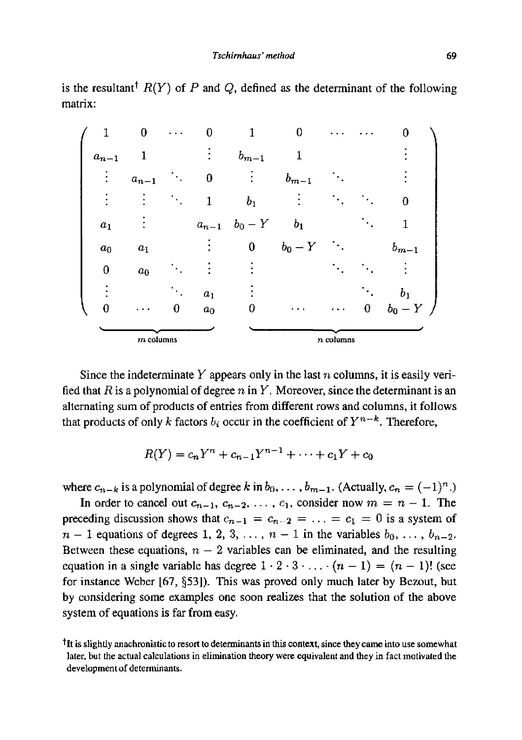
6.4 Tschirnhaus' method 67
Chapter? Roots of Unity 73
7.1 Introduction 73
7.2 The origin of de Moivre's formula 74
7.3 The roots of unity 81
7.4 Primitive roots and cyclotomic polynomials 86
Appendix: Leibniz and Newton on the summation of series 92
Exercises 94
Chapter 8 Symmetric Functions 97
8.1 Introduction 97
8.2 Waring's method 100
8.3 The discriminant 106
Appendix: Euler's summation of the series of reciprocals of perfect squares 110
Exercises 112
Chapter 9 The Fundamental Theorem of Algebra 115
9.1 Introduction 115
9.2 Girard's theorem 116
9.3 Proof of the fundamental theorem 119
Chapter 10 Lagrange 123
10.1 The theory of equations comes of age 123
10.2 Lagrange's observations on previously known methods 127
10.3 First results of group theory and Galois theory 138
Exercises 150

Contents xiii
Chapter 11 Vandermonde 153
I I.I Introduction 153
11.2 The solution of general equations 154
11.3 Cyclotomic equations 158
Exercises 164
Chapter 12 Gauss on Cyclotomic Equations 167
12.1 Introduction 167
12.2 Number-theoretic preliminaries 168
12.3 Irreducibility of the cyclotomic polynomials of prime index 175
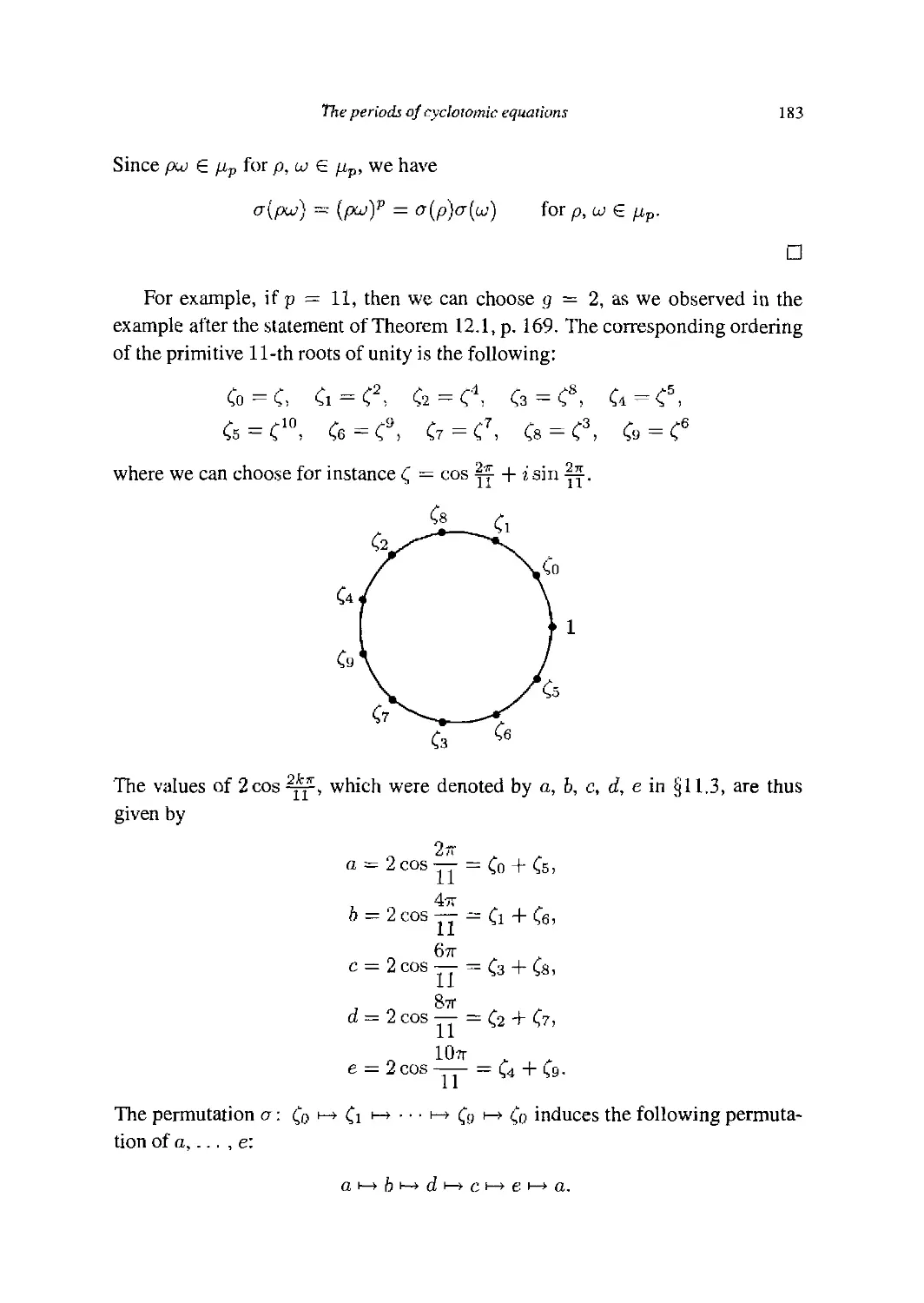
12.4 The periods of cyclotomic equations 182
12.5 Solvability by radicals 192
12.6 Irreducibility of the cyclotomic polynomials 196
Appendix: Ruler and compass construction of regular polygons 200
Exercises 206
Chapter 13 Ruffini and Abel on General Equations 209
13.1 Introduction 209
13.2 Radical extensions 212
13.3 Abel's theorem on natural irrationalities 218
13.4 Proof of the unsolvability of general equations of degree higher than 4 225
Exercises 227
Chapter 14 Galois 231
14.1 Introduction 231
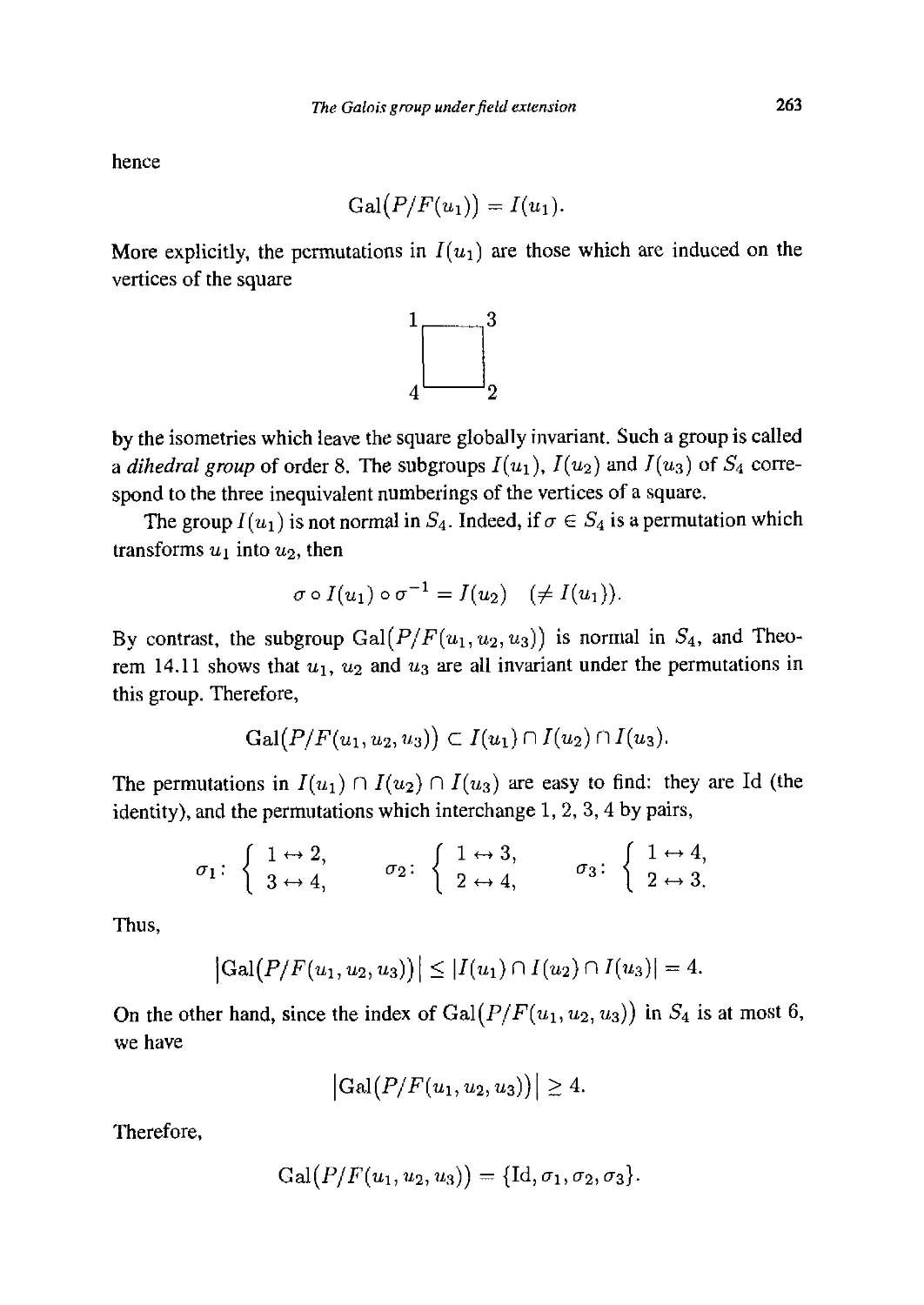
14.2 The Galois group of an equation 235
14.3 The Galois group under field extension 254
14.4 Solvability by radicals 264
14.5 Applications 281
Appendix: Galois' description of groups of permutations 295
Exercises 301
Chapter 15 Epilogue 303
Appendix: The fundamental theorem of Galois theory 307
Exercises 315
Selected Solutions 317
Bibliography 325
Index 331

Chapter 1
Quadratic Equations
1.1 Introduction
Since the solution of a linear equation aX = b does not use anything more than
a division, it hardly belongs to the algebraic theory of equations; it is therefore
appropriate to begin these lectures with quadratic equations
aX2 + bX + c = 0 (a ¿ 0).
Dividing both sides by a, we may reduce this to
X2+PX + q = 0.
The solution of this equation is well-known: when (§) is added to each side, the
square of X + | appears and the equation can be written
(*+!)'+-(!)'■
(This procedure is called "completion of the square"). The values of X easily
follow:
This formula is so well-known that it may be rather surprising to note that the
solution of quadratic equations could not have been written in this form before the
seventeenth century.* Nevertheless, mathematicians had been solving quadratic
*The first uniform solution for quadratic equations (regardless of the signs of coefficients) is due to
Simon Stevin in "L'Arithmetique" [55, p. 595], published in 1585. However, Stevin does not use
literal coefficients, which were introduced some years later by Francois Viéte: see chapter 4, §4.1.
1

2 Quadratic Equations
equations for about 40 centuries before. The purpose of this first chapter is to give
a brief outline of this "prehistory" of the theory of quadratic equations.
1.2 Babylonian algebra
The first known solution of a quadratic equation dates from about 2000 B.C.; on
a Babylonian tablet, one reads (see Van dcr Waerden [62, p, 69])
I have subtracted from the area the side of my square: 14.30.
Take 1, the coefficient. Divide 1 into two parts: 30. Multiply 30
and 30: 15. You add to J4.30, and 14.30.15 has the root 29.30.
You add to 29.30 the 30 which you have multiplied by itself: 30,
and this is the side of the square.
This text obviously provides a procedure for finding the side of a square (say
x) when the difference between the area and the side (i.e. x2 — x) is given; in
other words, it gives the solution of x2 — x = b.
However, one may be puzzled by the strange arithmetic used by Babylonians.
It can be explained by the fact that their base for numeration is 60; therefore 14.30
really means 14 • 60 + 3d, i.e. 870. Moreover, they had no symbol to indicate the
absence of a number or to indicate that certain numbers are intended as fractions.
For instance, when 1 is divided by 2, the result which is indicated as 30 really
means 30 ■ 60^1, i.e. 0.5, The square of this 30 is then 15 which means 0.25,
and this explains why the sum of 14,30 and 15 is written as 14,30.15: in modern
notations, the operation is 870 + 0,25 = 870.25.
After clearing the notational ambiguities, it appears that the author correctly
solves the equation x1 - x = 870, and gets x = 30. The other solution x = —29
is neglected, since the Babylonians had no negative numbers.
This lack of negative numbers prompted Babylonians to consider various types
of quadratic equations, depending on the signs of coefficients. There are three
types in all:
X2 + aX = b, X2 - aX = b, and X2 + b = aX,
where a, b stand for positive numbers. (The fourth type X2 4- aX +6 = 0
obviously has no (positive) solution.)
Babylonians could not have written these various types in this form, since
they did not use letters in place of numbers, but from the example above and from
other numerical examples contained on the same tablet, it clearly appears that the

Babylonian algebra
Babylonians knew the solution of
X2+aX=b as
2 L a
and of
X — aX = b as X =
How they argued to get these solutions is not known, since in every extant exam-
example, only the procedure to find the solution is described, as in the example above.
It is very likely that they had previously found the solution of geometric problems,
such as to find the length and the breadth of a rectangle, when the excess of the
length on the breadth and the area are given. Letting x and y respectively denote
the length and the breadth of the rectangle, this problem amounts to solving the
system
I x-y=a
\ xy = b.
By elimination of y, this system yields the following equation for x:
If x is eliminated instead of y, we get
y2 + ay = b.
A.1)
A.2)
A.3)
Conversely, equations A.2) and A.3) are equivalent to system A.1) after setting
y — x — a or x = y + a.
They probably deduced their solution for quadratic equations A.2) and A.3)
from their solution of the corresponding system A.1), which could be obtained as
follows: let z be the arithmetic mean of x and y.

4 Quadratic Equations
In other words, z is the side of the square which has the same perimeter as the
given rectangle:
a a
z = x-- = y+-.
Compare then the area of the square (i.e. z2) to the area of the rectangle (xy = b).
We have
whence b = z2 - (f J. Therefore, z = yj (§J + b and it follows that
a ,
- and
a
-.
This solves at once the quadratic equations x2 — ax = b and y2 + ay = b.
Looking at the various examples of quadratic equations solved by Babyloni-
Babylonians, one notices a curious fact: the third type x2 + b = ax does not explicitly
appear. This is even more puzzling in view of the frequent occurrence in Babylo-
Babylonian tablets of problems such as to find the length and the breadth of a rectangle
when the perimeter and the area of the rectangle are given; which amounts to the
solution of
x + y — a
xy = b.
A.4)
By elimination of y, this system leads to x2 + b = ax. So, why did Babylonians
solve the system A.4) and never consider equations like x2 + b — axl
A clue can be discovered in their solution of system A.4), which is probably
obtained by comparing the rectangle with sides x, y to the square with perimeter
a.
2'
■(!-*)■
One then sets x = | + z, whence y — | - z, and finishes as before.

Greek algebra
Whatever their method, the solution they get is
thus assigning one value for x and one value for y, while it is clear to us that x
and y are interchangeable in the system A.4): we would have given two values
for each one of the unknown quantities, and found
In the Babylonian phrasing, however, x and y are not interchangeable: they are
the length and the breadth of a rectangle, so there is an implicit condition that
x > y. According to S. Gandz [22, §9], the type X2 + b — aX was systematically
and purposely avoided by Babylonians because, unlike the two other types, it has
two positive solutions (which are the length x and the breadth y of the rectangle).
The idea of two values for one quantity was probably very embarrassing to them,
it would have struck Babylonians as an illogical absurdity, as sheer nonsense.
However, this observation that algebraic equations of degree higher than 1
have several interchangeable solutions is of fundamental importance: it is the
corner-stone of Galois theory, and we shall have the opportunity to see to what
clever use it will be put by Lagrange and later mathematicians.
As Andre Weil commented in relation to another topic [69, p. 104]
This is very characteristic in the history of mathematics. When
there is something that is really puzzling and cannot be under-
understood, it usually deserves the closest attention because some time
or other some big theory will emerge from it.
1.3 Greek algebra
The Greeks deserve a prominent place in the history of mathematics, for being
the first to perceive the usefulness of proofs. Before them, mathematics were
rather empirical. Using deductive reasoning, they built a huge mathematical mon-
monument, which is remarkably illustrated by Euclid's celebrated masterwork "The
Elements" (c. 300 B.C.).

Quadratic Equations
The Greeks' major contribution to algebra during this classical period is foun-
dational. They discovered that the naive idea of number (i.e. integer or rational
number) is not sufficient to account for geometric magnitudes. For instance, there
is no line segment which could be used as a length unit to measure the diagonal
and the side of a square by integers: the ratio of the diagonal to the side (i.e. V^)
is not a rational number, or in other words, the diagonal and the side are incom-
incommensurable.
The discovery of irrational numbers was made among followers of Pythago-
Pythagoras, probably between 430 and 410 B.C. (see Knorr [39, p. 49]). It is often credited
to Hippasus of Metapontum, who was reportedly drowned at sea for producing a
downright counterexample to the Pythagoreans' doctrine that "all things are num-
numbers." However, no direct account is extant, and how the discovery was made is
still a matter of conjecture. It is widely believed that the first magnitudes which
were shown to be incommensurable are the diagonal and the side of a square, and
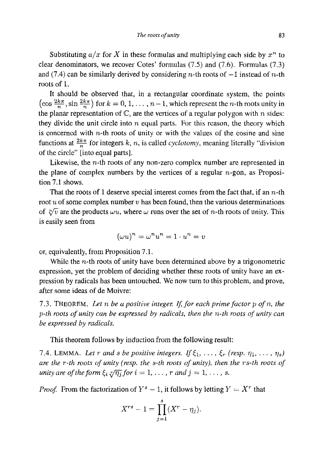
the following reconstruction of the proof has been proposed by Knorr [39, p. 27]:
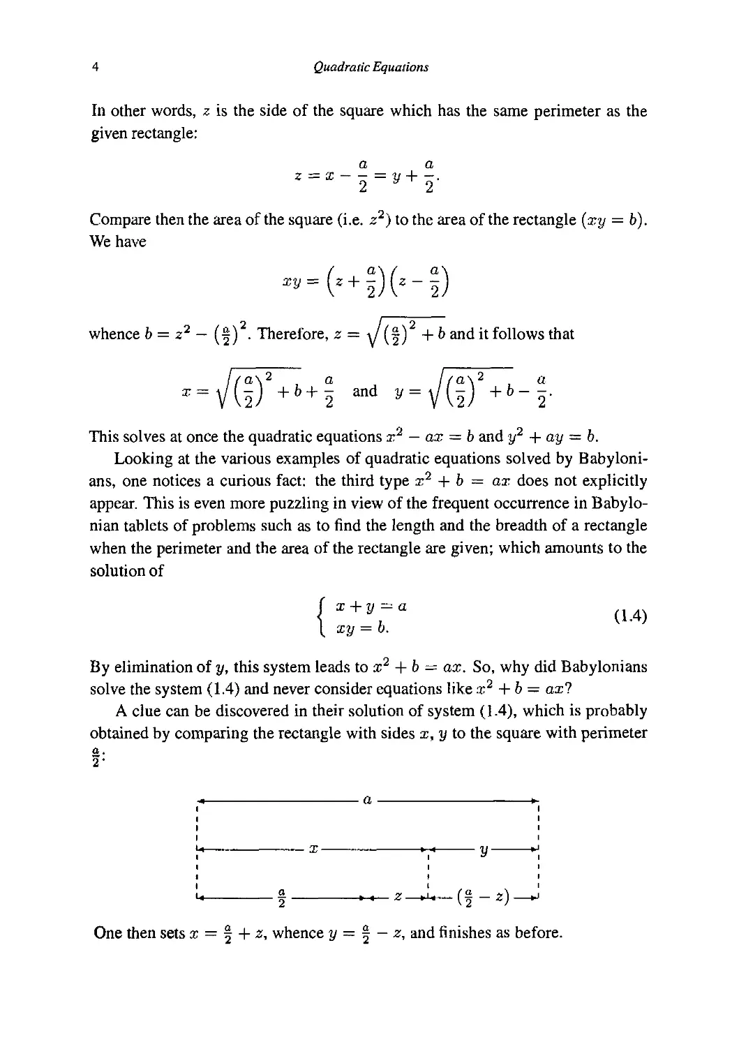
Assume the side AB and the diagonal AC of the square ABCD are both
measured by a common segment; then AB and AC both represent numbers (= in-
integers) and the squares on them, which are ABCD and EFGH, represent square
numbers. From the figure, it is clear (by counting triangles) that EFGH is the
double of ABCD, so EFGH is an even square number and its side EF is there-
therefore even. It follows that EB also represents a number, whence EBKA is a
square number.
H
D
G
A
A1
E
/ D'
K \
a /
B'
B
Since the square ABCD clearly is the double of the square EBKA, the same
arguments show that AB is even, whence A'B' represents a number.

Greek algebra 7
We now see that A'B' and A'C (= EB), which are the halves of AB and
AC, both represent numbers; but A'B1 and A'C are the side and the diagonal of
a new (smaller) square, so we may repeat the same arguments as above.
Iterating this process, we see that the numbers represented by AB and AC are
indefinitely divisible by 2. This is obviously impossible, and this contradiction
proves that AB and AC are incommensurable.
This result obviously shows that integers are not sufficient to measure lengths
of segments. The right level of generality is that of ratios of lengths. Prompted
by this discovery, the Greeks developed new techniques to operate with ratios
of geometric magnitudes in a logically coherent way, avoiding the problem of
assigning numerical values to these magnitudes. They thus created a "geometric
algebra," which is methodically taught by Euclid in "The Elements."
By contrast, Babylonians seem not to have been aware of the theoretical dif-
difficulties arising from irrational numbers, although these numbers were of course
unavoidable in the treatment of geometric problems: they simply replaced them
by rational approximations. For instance, the following approximation of V2 has
been found on some Babylonian tablet: 1.24.51.10, i.e. 1 + 24 ■ Q0~l + 51 • 6CT2 +
10 • 60~3 or 1.41421296296296..., which is accurate up to the fifth place.
Although Euclid does not explicitly deal with quadratic equations, the solution
of these equations can be detected under a geometric garb in some propositions of
the Elements. For instance, Proposition 5 of Book II states [30, v. I, p. 382]:
If a straight line be cut into equal and unequal segments, the rect-
rectangle contained by the unequal segments of the whole together
with the square on the straight line between the points of section
is equal to the square on the half.
-y-
A
K
C D
a
2
L
z
§-*
H
B
M
E
G

8 Quadratic Equations
On the figure above, the straight line AB has been cut into equal segments at
C and unequal segments at D, and the proposition asserts that the rectangle AH
together with the square LG (which is equal to the square on CD) is equal to the
square CF. (This is clear from the figure, since the rectangle AL is equal to the
rectangle DF).
If we understand that the unequal segments in which the given straight line
AB = a is cut are unknown, it appears that this proposition provides us with the
core of the solution of the system
( x + y- a
\ xy = b.
Indeed, setting z = x — | "the straight line between the points of section," it states
that b -f z2 = (|J. It then readily follows that
z =
) -b and ^2-
whence
as in Babylonian algebra. In subsequent propositions, Euclid also teaches the
solution of
x — y = a
xy = b
which amounts to x2 — ax = b or y2 + ay = b. He returns to the same type
of problems, but in a more elaborate form, in propositions 28 and 29 of book VI
(Compare Kline [38, pp. 76-77] and Van der Waerden [62, p. 121].)
The Greek mathematicians of the classical period thus reached a very high
level of generality in the solution of quadratic equations, since they considered
equations with (positive) real coefficients. However, geometric algebra, which
was the only rigorous method of operating with real numbers before the XlXth
century, is very difficult. It imposes tight limitations which are not natural from the
point of view of algebra; for instance, a great skill in the handling of proportions
is required to go beyond degree three.
To progress in the theory of equations, it was necessary to think more about
formalism and less about the nature of coefficients. Although later Greek math-
mathematicians such as Hero and Diophantus took some steps in that direction, the

Arabic algebra 9
really new advances were brought by other civilizations. Hindus, and Arabs later,
developed techniques of calculation with irrational numbers, which they treated
unconcernedly, without worrying about their irrationality. For instance, they were
familiar with formulas like
±b + 2\(ab
which they obtained from (u + vJ = u2 + v2 + 2uv by extracting roots of both
sides and replacing u and v by y/a and Vb respectively. Their notion of math-
mathematical rigor was rather more relaxed than that of Greek mathematicians, but
they paved the way to a more formal (or indeed algebraic) approach to quadratic
equations (see Kline [38, ch. 9, §2]).
1.4 Arabic algebra
The next landmark in the theory of equations is the book "Al-jabr w' al muqabala"
(c. 830 A.D.), due to Mohammed ibn Musa al-Khowarizmi.
The title refers to two basic operations on equations. The first is al-jabr (from
which the word "algebra" is derived) which means "the restoration" or "making
whole." In this context, it stands for the restoration of equality in an equation by
adding to one side a negative term which is removed from the other. For instance,
the equation
x2 = 40x - 4x2
is converted into
5x2 = 40x
by al-jabr [36, p. 105]. The second basic operation al muqabala means "the
opposition" or "balancing"; it is a simplification procedure by which like terms
are removed from both sides of an equation. For instance, al muqabala changes
50 + x2 = 29 + lOx
into
21 + x2 = lOx
[36, p. 109],

10 Quadratic Equations
In this work, al-Khowarizmi initiates what might be called the classical period
in the theory of equations, by reducing the old methods for solving equations
to a few standardized procedures. For instance, in problems involving several
unknowns, the systematically sets up an equation for one of the unknowns, and he
solves the three types of quadratic equations
X + aX = 6, X2 + b = aX, X2 =aX + b
by completion of the square, giving the two (positive) solutions for the type X1 +
b = aX.
Al-Khowarizmi first explains the procedure, as a Babylonian would have done:
The following is an example of squares and roots equal to
numbers: a square and 10 roots are equal to 39 units. The ques-
question therefore in this type of equation is about as follows: what
is the square which combined with ten of its roots will give a
sum total of 39? The manner of solving this type of equation is
to take one-half of the roots just mentioned. Now the roots in the
problem before us are 10. Therefore take 5, which multiplied by
itself gives 25, an amount which you add to 39, giving 64.
Having taken then the square root of this which is 8, sub-
subtract from it the half of the roots, 5, leaving 3. The number
three therefore represents one root of this square, which itself,
of course, is 9. Nine therefore gives that square. [36, pp. 71-73]
However, after explaining the procedure for solving each of the six types
mX2 = aX, mX2 = b, aX = b, mX2 + aX = b, mX2 + b = aX and
mX2 = aX + b, he adds:
We have said enough, says Al-Khowarizmi, so far as num-
numbers are concerned, about the six types of equations. Now, how-
however, it is necessary that we should demonstrate geometrically
the truth of the same problems which we have explained in num-
numbers. [36, p. 77]
He then gives geometric justifications for his rules for the last three types,
using completion of the square as in the following example for x2 + 10.-r = 39:

Arabic algebra
5 x A
ll
G
25
B
c
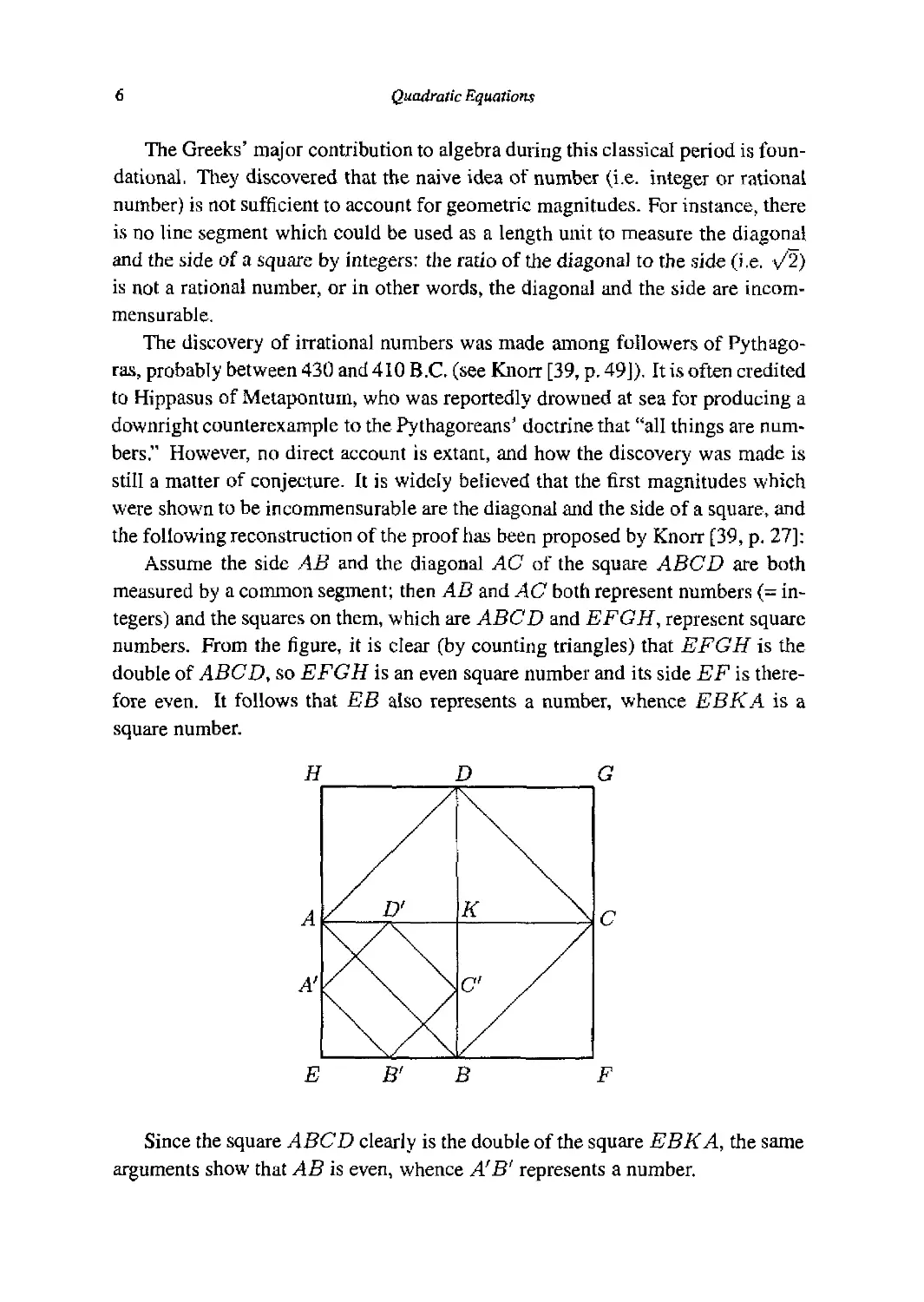
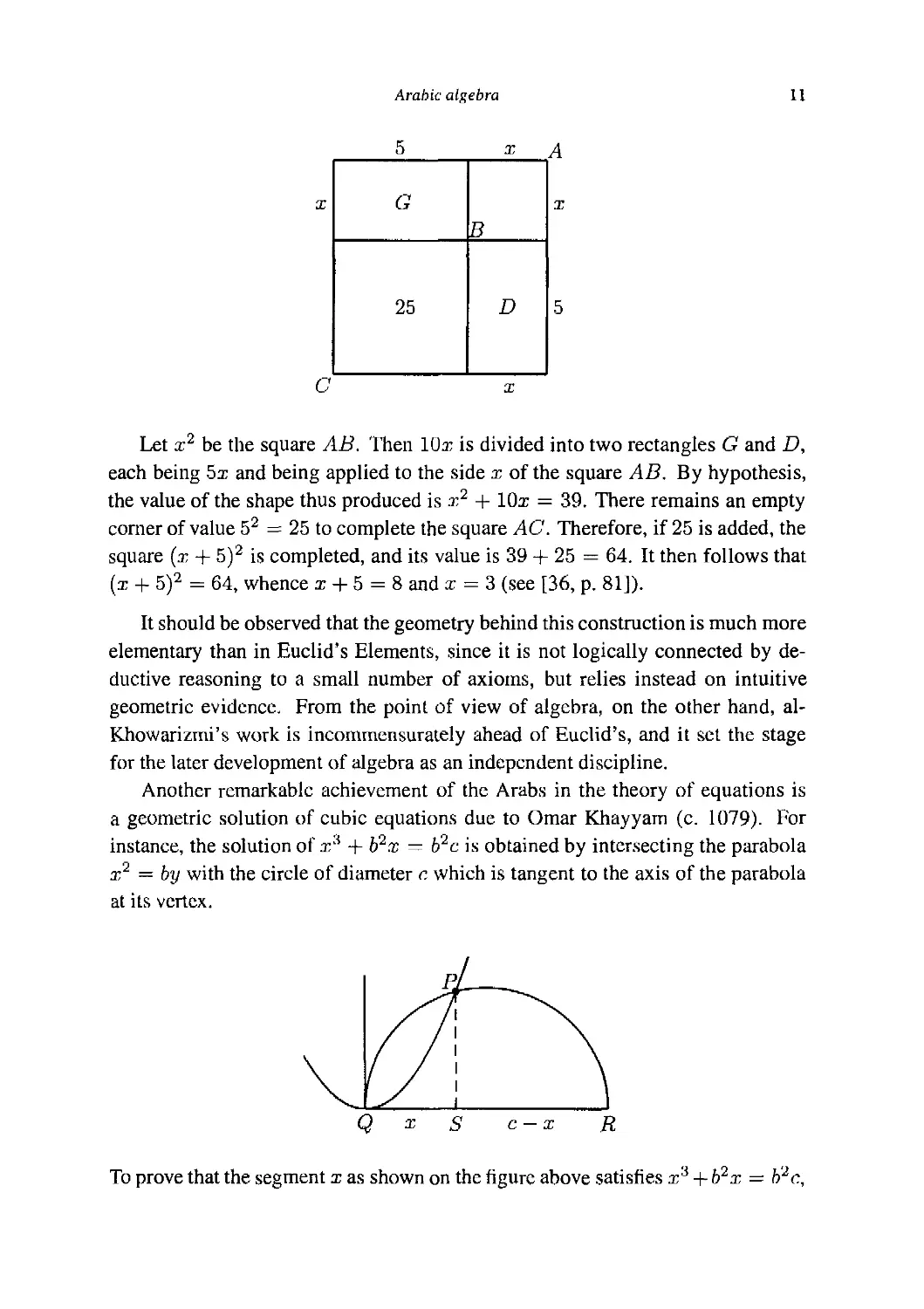
Let a;2 be the square AB. Then 10a; is divided into two rectangles G and D,
each being 5x and being applied to the side x of the square AB. By hypothesis,
the value of the shape thus produced is x? + lOx = 39. There remains an empty
corner of value 52 = 25 to complete the square AC. Therefore, if 25 is added, the
square (a; + 5J is completed, and its value is 39 + 25 = 64. It then follows that
(x + 5J = 64, whence x + 5 = 8anda; = 3 (see [36, p. 81]).
It should be observed that the geometry behind this construction is much more
elementary than in Euclid's Elements, since it is not logically connected by de-
deductive reasoning to a small number of axioms, but relies instead on intuitive
geometric evidence. From the point of view of algebra, on the other hand, al-
Khowarizmi's work is incommensurately ahead of Euclid's, and it set the stage
for the later development of algebra as an independent discipline.
Another remarkable achievement of the Arabs in the theory of equations is
a geometric solution of cubic equations due to Omar Khayyam (c. 1079). For
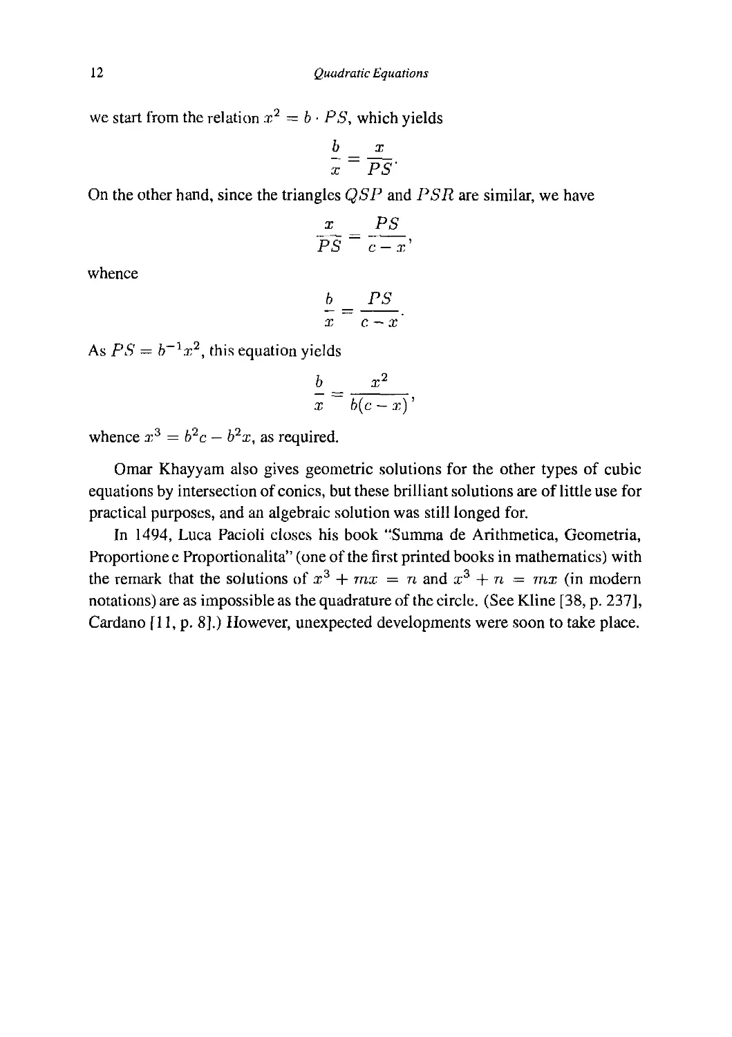
instance, the solution of a;3 + b2x = b2c is obtained by intersecting the parabola
x2 = by with the circle of diameter c which is tangent to the axis of the parabola
at its vertex.
Q x S c-x R
To prove that the segment x as shown on the figure above satisfies x'3 + b2x = b'2c,

12 Quadratic Equations
we start from the relation x2 = b ■ PS, which yields
b x
On the other hand, since the triangles QSP and PSR are similar, we have
_x^ _ _PS_
PS~c-x
whence
6 PS
x c - x
As PS — b~1x2, this equation yields
x b(c — x)'
whence x3 = b2c — b2x, as required.
Omar Khayyam also gives geometric solutions for the other types of cubic
equations by intersection of conies, but these brilliant solutions are of little use for
practical purposes, and an algebraic solution was still longed for.
In 1494, Luca Pacioli closes his book "Summa de Arithmetica, Geometria,
Proportione e Proportionalita" (one of the first printed books in mathematics) with
the remark that the solutions of x3 + mx = n and a;3 + n = mx (in modern
notations) are as impossible as the quadrature of the circle. (See Kline [38, p. 237],
Cardano f 11, p. 8].) However, unexpected developments were soon to take place.

Chapter 2
Cubic Equations
2.1 Priority disputes on the solution of cubic equations
The algebraic solution of X3 + mX — n was first obtained around 1515 by
Scipione del Ferro, professor of mathematics in Bologna. Not much is known
about him nor about his solution as, for some reason, he decided not to publicize
his result. After his death in 1526, his method passed to some of his pupils.
The second discovery of the solution is much better known, through the ac-
accounts of its author himself, Niccolo Fontana (c. 1500-1557), from Brescia, nick-
nicknamed 'Tartaglia" ("Stammerer") (see Hankel [28, pp. 360ff]). In 1535, Tartaglia,
who had dealt with some very particular cases of cubic equations, was challenged
to a public problem-solving contest by Antonio Maria Fior, a former pupil of
Scipione del Ferro. When he heard that Fior had received the solution of cubic
equations from his master, Tartaglia threw all his energy and his skill into the
struggle. He succeeded in finding the solution just in time to inflict upon Fior a
humiiiating defeat.
The news that Tartaglia had found the solution of cubic equations reached
Girolamo Cardano A501-1576), a very versatile scientist, who wrote a number
of books on a wide variety of subjects, including medicine, astrology, astronomy,
philosophy and mathematics. Cardano then asked Tartaglia to give him his so-
solution, so that he could include it in a treatise on arithmetic, but Tartaglia flatly
refused, since he was himself planning to write a book on this topic. It turns out
that Tartaglia later changed his mind, at least partially, since in 1539 he handed
on to Cardano the solution of X3 + mX = n, X:i = mX + n and a very brief
indication on X3 + n — mX in verses* (see Hankel [28, pp. 364-365]):
*As pointed out by Boorstin (cited by Weeks [66, p. Ix]), verses were a useful memorization aid at a
13

14 Cubic Equations
Quando che'I cubo con le cose appresso
Se agguaglia a qualche numero discreto:
Trovan dui altri, dijferenti in esso.
Dapoi terrai, questo per consueto,
Che'i lorprodutto, sempre sia eguale
Al terzo cubo delle cose neto;
El residuo poi suo genérale,
Belli lor lati cubi, bene sottratti
Varra la tua cosa principale.
This excerpt gives the formula for X3 + rnX = n. The equation is indicated
in the first two verses: the cube and the things equal to a number. Cosa (- thing)
is the word for the unknown. To express the fact that the unknown is multiplied
by a coefficient, Tartaglia simply uses the plural form le cose. He then gives the
following procedure: find two numbers which differ by the given number and such
that their product is equal to the cube of the third of the number of things. Then
the difference between the cube roots of these numbers is the unknown.
With modern notations, we would write that, to find the solution of
X3 + mX = n,
we only need to find t, u such that
/m\3
t — u = n and tu = [ — 1 ;
\ o /
then
The values of i and u are easily found (see the system A.1), p. 3)
7Ti\J n
j) +2
2/
time when paper was expensive.

Cardano 's formula 15
Therefore, a solution of X3 + rnX = n is given by the following formula:
However, the poem does not provide any justification for this formula. Of course,
it "suffices" to check that the value of X given above satisfies the equation X3 +
mX = n, but this was far from obvious to a sixteenth century mathematician.
The major difficulty was to figure out that
(a - bf = a3 - 3a?b + 3ab2 - b3,
a formula which could be properly proved only by dissection of a cube in three-
dimensional space.
Having received Tartaglia's poem, Cardano set to work; he not only found
justifications for the formulas but he also solved all the other types of cubics. He
then published his results, giving due credit to Tartaglia and to del Ferro, in the
epoch-making book "Ars Magna, sive de regulis algebraicis" (The Great Art, or
the Rules of Algebra [11]). A bitter quarrel then erupted between Tartaglia and
Cardano, the former claiming that Cardano had solemnly sworn never to publish
Tartaglia's solution, while the latter countered that there had never been any ques-
question of secrecy.
2.2 Cardano's formula
Although Cardano lists 13 types of cubic equations and gives a detailed solution
for each of them, we shall use modern notations in this section, and explain Car-
Cardano's method for the general cubic equation
Xs + aX2 + bX + c = 0.
First, the change of variable Y = X + | converts the equation into one which
lacks the second degree term:
q = 0 B.1)
where
= b-j and g = c-|6 + 2(|). B.2)

16 Cubic Equations
If Y = ffi+ y/u, then
i = í + u + o\tuy vf -
and equation B.1) becomes
(t + u + q) + {3\Ziü + p){\Tt + ?/u) =0.
This equation clearly holds if the rational part t + u + q and the irrational part
(v^i + ^/u)(Z\/iu + p) both vanish or, in other words, if
This system has the solution
(see A.4), p. 4); hence a solution for equation B.1) is
B-3)
and a solution for the initial equation X3 + aX2 + bX + c = 0 easily follows by
substituting for p and q the expressions given by B.2). Equation B.3) is known as
Cardano's formula for the solution of the cubic B.1).
2.3 Developments arising from Cardano's formula
The solution of cubic equations was a remarkable achievement, but Cardano's for-
formula is far less convenient than the corresponding formula for quadratic equations
since it has some drawbacks which undoubtedly baffled XVI-th century mathe-
mathematicians (to begin with, its discoverers).
(a) First, when some solution is expected, it is not always yielded by Cardano's
formula. This could have struck Cardano when he was devising examples for
illustrating his rules, such as
X3 + 16 = \2X

Developments arising from Cardano's formula 17
(see Cardano [11, p. 12]) which is constructed to give 2 as an answer. Cardano's
formula yields
X= \^8+ ^=8 = -4.
Why does it yield -4 and not 2?
It is likely that the above observation had first prompted Cardano to investi-
investigate a question much more interesting to him: How many solutions does a cubic
equation have? He was thus led to observe that cubic equations may have three so-
solutions (including the negative ones, which Cardano terms "false" or "fictitious,"
but not the imaginary ones) and to investigate the relations between these solutions
(see Cardano [11, Chapter I]).
(b) Next, when there is a rational solution, its expression according to Cardano's
formula can be rather awkward. For instance, it is easily seen that 1 is solution of
X3 + X = 2,
but Cardano's formula yields
Now, the equation above has only one real root, since the function f(X) = X3 +
X is monotonically increasing (as it is the sum of two monotonically increasing
functions) and, therefore, takes the value 2 only once. We are thus compelled to
conclude
a rather surprising result.
Already in 1540, Tartaglia tried to simplify the irrational expressions arising
in his solution of cubic equations (see Hankel [28, p. 373]). More precisely, he
tried to determine under which condition an irrational expression like y a + \Jb
could be simplified to u + -Jv. This problem can be solved as follows (in modern
notations): starting with
y a + Vb - u + y/v B.5)
and taking the cube of both sides, we obtain
a+ Vb = u3 + 3uv + Cu2 +

18
Cubic Equations
whence, equating separately the rational and the irrational parts (this is licit if a,
i>, u and v are rational numbers),
a — u3 + 2>uv
B.6)
Subtracting the second equation from the first, we then obtain
a - \fb = (u - i/vK
whence
y a— vb = u — \/v.
Multiplying B.5) and B.7), we obtain
v/a2 - b — u2 — v
B.7)
B.8)
B.9)
which can be used to eliminate v from the first equation of system B.6). We thus
get
Therefore, if a and b are rational numbers such that v'o,2 — b is rational and if the
equation
4u3 - 3( \/a2 - b)u = a
has a rational solution u, then
\J a + vb = u + \/v and ya — vb = u — y/v,
where v is given by equation B.8)
v = u2 — {/a2 — b.
This effectively provides a simplification in the irrational expressions
which appear in Cardano's formula for the solution of X3 + pX + q = 0, but
this simplification is useless as far as the solution of cubic equations is concerned.

Developments arising from Cardarlo 'íformula 19
Indeed, if a — —| and b = (§) + (§) , one has to find a rational solution of
equation B.9):
and this exactly amounts to finding a rational solution of the initial equation X3 +
pX + g = 0, since these equations are related by the change of variable X = 2u.
However, this process can be used to show, for instance, that
1 i 1 / '! A .i/]__2/I_I_l jl
•i y 3 '2 2 y 3
from which formula B.4) follows.
(c) The most serious drawback of Cardano's formula appears when one tries to
solve an equation like
X3 = 15X + 4.
It is easily seen that X = 4 is a solution, but Cardano's formula yields a very
embarrassing expression:
X =
in which square roots of negative numbers are extracted. The case where (|) +
(|J < 0 is known as the "casus irreducibilis" of cubic equations. For a long
time, the validity of Cardano's formula in this case had been a matter of debate,
but the discussion of this case had a very important by-product: it prompted the
use of complex numbers.
Complex numbers had been, up to then, brushed aside as absurd, nonsensical
expressions. A remarkably explicit example of this attitude appears in the follow-
following excerpt from chapter 37 of the Ars Magna [11, p. 219]:
If it should be said, Divide 10 into two parts the product of which
is 30 or 40, it is clear that this case is impossible. Nevertheless,
we will work thus: ...
Cardano then applies the usual procedure with the given data, which amounts to
solving X2 - 10X + 40 = 0, and comes up with the solution: these parts are
5 + \J—15 and 5 — %/—15. He then justifies his result:

20 Cubic Equations
Putting aside the mental tortures involved,* multiply 5 + \/-15
by 5 - "/-15, making 25 — (—15) which is +15. Hence this
product is 40. [ ... ] So progresses arithmetic subtlety the end
of which, as is said, is as refined as it is useless.
However, with the "casus irreducibilis" of cubic equations, complex numbers
were imposed upon mathematicians. The operations on these numbers are clearly
taught, in a nearly modern way, by Rafaele Bombelli (c. 1526-1573), in his influ-
influential treatise: "Algebra" A572). In this book, Bombelli boldly applies to cube
roots of complex numbers the same simplification procedure as in (b) above, and
he obtains, for instance
y 2 + V-121 = 2 + -/^l and y
/-L21 = 2 - -/^l,
from which it follows that Cardano's formula gives indeed 4 for a solution of
A'3 = 15X + 4.
Complex numbers thus appeared, not to solve quadratic equations which lack
solutions (and do not need any), but to explain why Cardano's formula, efficient as
it may seen, fails in certain cases to provide expected solutions to cubic equations.
tin the original text: "dismissis incruciationibus." Perhaps Cardano played on words here, since an-
another translation for this passage is: "the cross-multiples having canceled out," referring to the fact
that in the product E + V—15)E — V—IS), the terms 5^—15 and —5^—15 cancel out.

Chapter 3
Quartic Equations
3.1 The unnaturalness of quartic equations
The solution of quartic equations was found soon after that of cubic equations. It
is due to Ludovico Ferrari A522-1565), a pupil of Cardano, and it first appeared
in the "Ars Magna."
Ferrari's method is very ingenious, relying mainly on transformation of equa-
equations, but it aroused less interest than the solution of cubic equations. This is
clearly shown by its place in the "Ars Magna": while Cardano spends thirteen
chapters to discuss the various cases of cubic equations, Ferrari's method is briefly
sketched in the penultimate chapter.
The reason for this relative disregard may be found in the introduction of the
"Ars Magna" [11, p. 9]:
Although a long series of rules might be added and a long dis-
discourse given about them, we conclude our detailed consideration
with the cubic, others being merely mentioned, even if gener-
generally, in passing. For as positio [the first power] refers to a line,
quadratum [the square] to a surface, and cubum [the cube] to
a solid body, it would be very foolish for us to go beyond this
point. Nature does not permit it.
This passage shows the equivocal status of algebra in the sixteenth century.
Its logical foundations were still geometric, as in the classical Greek period; in
this framework, each quantity has a dimension and only quantities of the same
dimension can be added or equated. For instance, an equation like x2 + b = ax
makes sense only if x and a are line segments and b is an area, and equations of
21

22 Quartic Equations
degree higher than three don't make any sense at all.*
However, from an arithmetical point of view, quantities are regarded as dimen-
sionless numbers, which can be raised to any power and equated unconcernedly.
This way of thought was clearly prevalent among Babylonians, since the very
statement of the problem: "I have subtracted from the area the side of my square:
14.30" is utter nonsense from a geometric point of view. The Arabic algebra
also stresses arithmetic, although al-Khowarizmi provides geometric proofs of his
rules (see §1.4).
In the "Ars Magna," both the geometric and the arithmetic approaches to equa-
equations are present. On one hand, Cardano tries to base his results on Euclid's "Ele-
"Elements," and on the other hand, he gives the solution of equations of degree 4. He
also solves some equations of higher degree, such as X9 + 3X6 + 10=15X3 [11,
p. 159], in spite of his initial statement that it would be "foolish" to go beyond de-
degree 3. However, the arithmetic approach, which would eventually predominate,
still suffered from its lack of a logical base until the early seventeenth century (see
§4.1).
3.2 Ferrari's method
In this section, we use modern notations to discuss Ferrari's solution of quartic
equations. Let
Xa
be an arbitrary quartic equation. By the change of variable Y = X + | the cubic
term cancels out, and the equation becomes
Y4+pY2+qY+ r = 0 C.1)
* A way out of this difficulty was eventually found by Descartes. In "La Geometrie" [16, p. 5], pub-
published in 1637, he introduces the following convention: if a unit line segment e is chosen, then the
square x2 of a line segment x is the side of the rectangle constructed on e which has the same area
as the square with side x. Thus, x2 is a line segment, and arbitrary powers of x can be interpreted as
line segments in a similar way.

Ferrari 's method 23
with
C.2,
Q,
r = d —-(
Moving the linear terms to the right-hand side and completing the square on the
left-hand side, we obtain
If we add a quantity u to the expression squared in the left-hand side, we get
iY2 + ?- + u) =-qY-r+(?-J + 2uY2+pu + u2. C.3)
The idea is to determine u in such a way that the right-hand side also becomes a
square. Looking at the terms in Y2 and in Y, it is easily seen that if the right-hand
side is a square, then it is the square of \f7hxY - —4=; therefore, we should have
C.4)
and, equating the independent terms, we see that this equation holds if and only if
or equivalently, after clearing the denominator and rearranging terms,
8u3 + 8pu2 + Bp2 - 8r)u - q2 = 0. C.5)
Therefore, by solving this cubic equation, we can find a quantity u for which
equation C.4) holds. Returning to equation C.3), we then have
whence
The values of Y are then obtained by solving the two quadratic equations above
(one corresponding to the sign + for the right-hand side, the other to the sign -).

24 Quartic Equations
To complete the discussion, it remains to consider the case where u = 0 is a
root of equation C.5), since the calculations above implicitly assume u / 0. But
this case occurs only if q = 0 and then the initial equation C.1) is
Y4+pY2 +r = 0.
This equation is easily solved, since it is a quadratic equation in Y2.
In summary, the solutions of
X4 + aX3 + bX2 + cX + d = 0
are obtained as follows: let p, q and r be defined as before (see C.2)) and let u be
a solution of C.5). If q ^ 0, the solutions of the initial quartic equation are
2 "V 2 2 2^ 4
where s and e' can be independently +1 or — 1. If q = 0, the solutions are
x = ew-?--'/^a
where e and s' can be independently +1 or -1.
Equation C.5), on which the solution of the quartic equation depends, is called
the resolvent cubic equation (relative to the given quartic equation). Depending
on the way equations are set up, one may come up with other resolvent cubic
equations. For instance, from equation C.1) one could pass to
(Y2 + vJ = (-PY2 -qY-r)+ 2vY2 + v2
where v is an arbitrary quantity (which plays the same role as | + u in the preced-
preceding discussion). The condition on v for the right-hand side to be a perfect square
is then
8vZ - 4pv2 - 8rv + Apr - q1 = 0. C.6)
After having determined v such that this condition holds, one finishes as before.
This second method is clearly equivalent to the previous one, by the change
of variable v — | + u. Therefore, equation C.6), which is obtained from C.5) by
this change of variable, is also entitled to be called the resolvent cubic.

Chapter 4
The Creation of Polynomials
4.1 The rise of symbolic algebra
In comparison to the rapid development of the theory of equations around the
middle of the sixteenth century, progress during the next two centuries was rather
slow. The solution of cubic and quartic equations was a very important break-
breakthrough, and it took some time before the circle of new ideas arising from these
solutions was fully explored and understood, and new advances were possible.
First of all, it was necessary to devise appropriate notations for handling equa-
equations. In the solution of cubic and quartic equations, Cardano was straining to
the utmost the capabilities of the algebraic system available to him. Indeed, his
notations were rudimentary: the only symbolism he uses consists in abbreviations
such as p : for "plus," m : for "minus" and 5R for "radix" (= root).
For instance, the equation X2 + 2X — 48 is written as
1. quad, p : 2 pos. aeq. 48
(quad, is for "quadratum," pos. for "positiones" and aeq. for "aequatur"), and
E + v/=:15)E - y/^TE) = 25 - (-15) = 40
is written (see Cajori [10, §140])
5p : SRm : 15
5m : 9?m : 15
25m : m : 15 qdest 4.0.
Using this embryonic notation, transformation of equations was clearly a tour
de force, and a more efficient notation had to develop in order to enlighten this
new part of algebra.
25

26 The Creation of Polynomials
This development was rather erratic. Advances made by some authors were
not immediately taken up by others, and the process of normalization of notations
took a long time. For example, the symbols + and - were already used in Ger-
Germany since the end of the fifteenth century (Cajori [10, §201]), but they were not
widely accepted before the early seventeenth century, and the sign = for equality,
first proposed by R. Recordé in 1557, had to struggle with Descartes' symbol x>
for nearly two centuries (Cajori [10, §267]).
These are relatively minor points, since it may be assumed that p :, m : and
aeq. were as convenient to Cardano as +, — and = are to us. There is one
point, however, where a new notation was vital. In effect, it helped create a new
mathematical object: polynomials. There is indeed a significant step from
1. quad, p : 2 pos. aeq. 48
which is the mere statement of a problem, to the calculation with polynomials like
X2 + 2X — 48, and this step was considerably facilitated by a suitable notation.
Significant as it may be, the evolution from equations to polynomials is rather
subtle, and leading mathematicians of this period rarely took the time to clarify
their views on the subject; the rise of the concept of polynomial was most often
overshadowed by its application to the theory of equations, and it can only be
gathered from indirect indications.
Two milestones in this evolution are "L'Arithmetique" A585) of Simon Stevin
A548-1620) and "In Artem Analyticem Isagoge" (= Introduction to the Analytic
Art) A591) of Francois Viéte A540-1603).
4.1.1 L'Arithmetique
This book combines notational advances made by Bombelli and earlier authors
(see Cajori [10, §296]) with theoretical advances made by Pedro Nunes A502-
1578) (see Bosnians [5, p. 165]) to present a comprehensive treatment of poly-
polynomials. Stevin's notation for polynomials, which he terms "multinomials" [55,
p. 521] or "integral algebraic numbers" [55, p. 518] (see also pp. 570 ff) has a
surprising touch of modernity: the indeterminate is denoted by (T), its square by
B), its cube by C), etc., and the independent term is indicated by @ (sometimes
omitted), so that a "multinomial" appears as an expression like
3C) + 5© -4® + 6@) (or3C) + 5B)-4® + 6).
Such an expression could be regarded (from a modern point of view) as a finite
sequence of real numbers, or, better, as a sequence of real numbers which are all

The rise ujsymbolic algebra 27
zero except for a finite number of them, or as a function from N to R with finite
support (compare §5.1).
This exponential notation (which was not unprecedented) probably helped to
aboJish the psychological barrier of the third degree (see §3.1), by placing all the
powers of the unknown on an equal footing. It is however rather unfortunate for
equations with several unknowns.
Most important is Stevin's observation that the operations on "integral alge-
algebraic numbers" share many features with those on "integral arithmetic numbers"
(= integers). In particular, he shows [55, Probleme 53, p. 577] that Euclid's algo-
algorithm for determining the greatest common divisor of two integers applies nearly
without change to find the greatest common divisor of two polynomials (see §5.2,
and particularly p. 44).
Although the concept of polynomial is quite clear, the way equations are set
up is rather awkward in "L'Arithmetique," since equations are replaced by pro-
proportions and the solution of equations is called by Stevin "the rule of three of
quantities." In modern notation, the idea is to replace the solution of an equation
like
X2 - aX - b = 0
by the following problem: find the fourth proportional u in
X2 X
aX + b u
or, more generally, find P(u) in
X2 __ P(X)
aX + b~ P{u) '
where P(X) is an arbitrary polynomial in X, see [55, p. 592]. (Of course, the
solutions which are equal to zero must then be rejected.)
In Stevin's words [55, p. 595]:
Given three terms, of which the first B), the second (T) @), the
third an arbitrary algebraic number: To find their fourth propor-
proportional term.
This fancy approach to equations may have been prompted by Stevin's me-
methodical treatment of polynomials: an equality like
X2 = aX + b

28 The Creation of Polynomials
would mean that the polynomials X2 and aX + b are equal; but polynomials are
equal if and only if the coefficients of similar powers of the unknown are the same
in both polynomials, and this is clearly not the case here, since X2 appears on
the left-hand side but not on the right-hand side. Stevin's own explanation [55,
pp. 581-582], while not quite convincing, at least shows that he was fully aware
of this notational difficulty:
The reason why we call rule of three, or invention of the fourth
proportional of quantities, that which is commonly called equa-
equation of quantities: [ .,, ] Because this word "equation" let the
beginners think that it was some singular matter, which how-
however is common in the usual arithmetic, since we seek to three
given terms a fourth proportional. As that, which is called equa-
equation, does not consist in the equality of absolute quantities, but
in equality of their values, so this proportion is concerned with
the value of quantities, as the same is usual in everyday life.
This approach met with little success. Even Albert Girard, the first editor of
Stevin's works, did not follow Stevin's set up in his own work, and it was soon
abandoned.
Stevin's formal treatment of polynomials is rather isolated too; in later works,
polynomials were most often considered as functions, although formal operations
like Euclid's algorithm were performed. For instance, here is the definition of an
equation according to Rene Descartes A596-1650) [16, p. 156]:
An equation consists of several terms, some known and some
unknown, some of which are together equal to the rest; or rather,
all of which taken together are equal to nothing; for this is often
the best form to consider.
A polynomial then appears as "the sum of an equation" [16, p. 159]. On the
whole, the idea of polynomial in the seventeenth century is not very different
from the modern notion, and the need for a more formal definition was not felt
for a long time, but one can get some feeling of the difference between Descartes'
view and ours from the following excerpt of "La Geometrie" A637) [16, p. 159]:
(the emphasis is mine)
Multiplying together the two eguaíi'oníz-2 = Oandx-3 = 0,
we have x2 - 5x + 6 = 0, or x2 = 5x - 6. This is an equation
in which x has the value 2 and at the same time the value 3.

The rise of symbolic algebra 29
4.1,2 In Artem Analyticem Isagoge
A major advance in notation with far-reaching consequences was Francois Viete's
idea, put forward in his "Introduction to the Analytic Art" A591), of designating
by letters all the quantities, known or unknown, occurring in a problem. Although
letters were occasionally used for unknowns as early as the third century A.D.
(by Diophantus of Alexandria, see Cajori [10, §101]), the use of letters for known
quantities was very new. It also proved to be very useful, since for the first time it
was possible to replace various numerical examples by a single "generic" exam-
example, from which all the others could be deduced by assigning values to the letters.
However, it should be observed that this progress did not reach its full extent in
Viete's works, since Viete completely disregards negative numbers; therefore, his
letters always stand for positive numbers only.
This slight limitation notwithstanding, the idea had another important conse-
consequence: by using symbols as his primary means of expression and showing how
to calculate with those symbols, Viéte initiated a completely formal treatment of
algebraic expressions, which he called logistice speciosa [65, p. 17] (as opposed
to the logistice numerosa, which deals with numbers). This "symbolic logistic"
gave some substance, some legitimacy to algebraic calculations, which allowed
Viéte to free himself from the geometric diagrams used so far as justifications.
However, Viete's calculations are somewhat hindered by his insistence that
each coefficient in an equation be endowed with a dimension, in such a way that
all the terms have the same dimension: the "prime and perpetual law of equations"
is that "homogeneous terms must be compared with homogeneous terms" [65,
p. 15]. Moreover, Viete's notation is not as advanced as it could be, since he does
not use numerical exponents. For instance, instead of
Let A3 + WA = 2Z,
Viéte writes {see Cajori [10, §177])
Proponatur A cubus + B piano 3 in A aequari Z solido 2,
insisting that B and Z have degree 2 and 3 respectively.
These minor flaws were soon corrected. In "La Geometrie" A637) [16], Rene
Descartes shaped the notation that is still in use today (except for his above-
mentioned sign x> for equality). Thus, in less than one century, algebraic notation
had dramatically improved, reaching the same level of generality and the same
versatility as ours. These notational advances fostered a deeper understanding of
the nature of equations, and the theory of equations was soon advanced in some

30
The Creation of Polynomials
important points, such as the number of roots and the relations between roots and
coefficients of an equation.
4.2 Relations between roots and coefficients
Cardano's observations on the number of roots of cubic and quartic equations (see
§2.3) were substantially generalized during the next century. Progress in plane
trigonometry brought rather unexpected insights into this question.
In 1593, at the end of the preface of his book "Ideae Mathematicae" [48]
(see also Goldstine [27, §1.6]), Adriaan van Roomen* A561-1615) issued the
following challenge to "all the mathematicians throughout the whole world":
Find the solution of the equation
45X - 3795X3 + 95634X5 - 1138500X7 + 7811375X9 - 34512075X11
+ 105306075X13 - 232676280X15 + 384942375X17 - 488494125X19
+ 483841800X21 - 378658800X23 + 236030652X25 - 117679100X27
+ 4G955700X29 - 14945040X31 + 3764565X33 - 740259A'35
+ 111150X37 - 12300X3" + 945X41 - 45X43 + X45 = A.
He gave the following examples, the second of which is erroneous:
(a) if A =
(b)if.4 =
\/2, then X
= y 2 - y 2 + \J2
\
[it should be A =
then X =
[it should be X =
\
2 - t/2
*lhen professor at the University of Lou vain.

Relations between roots and coefficients 31
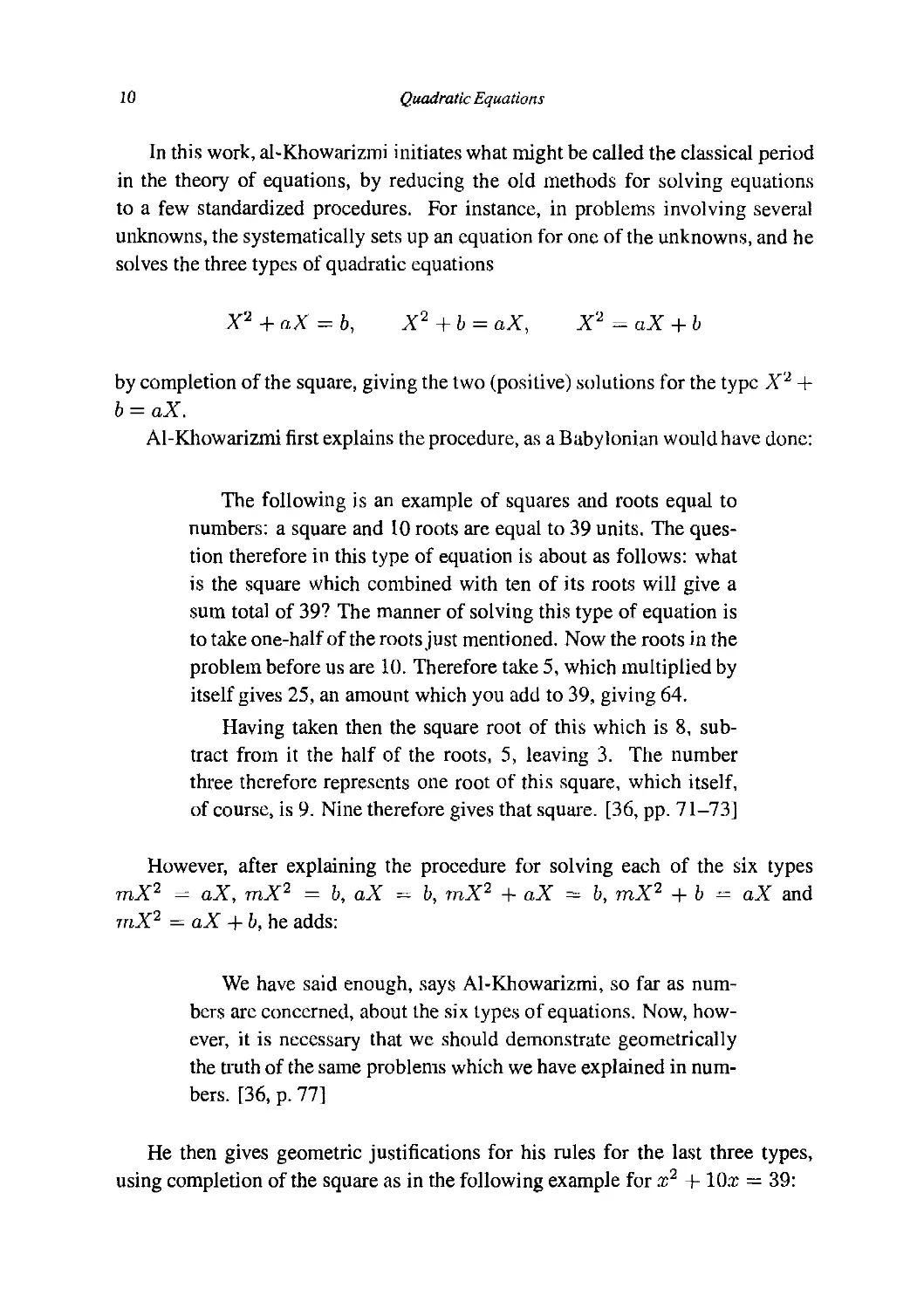
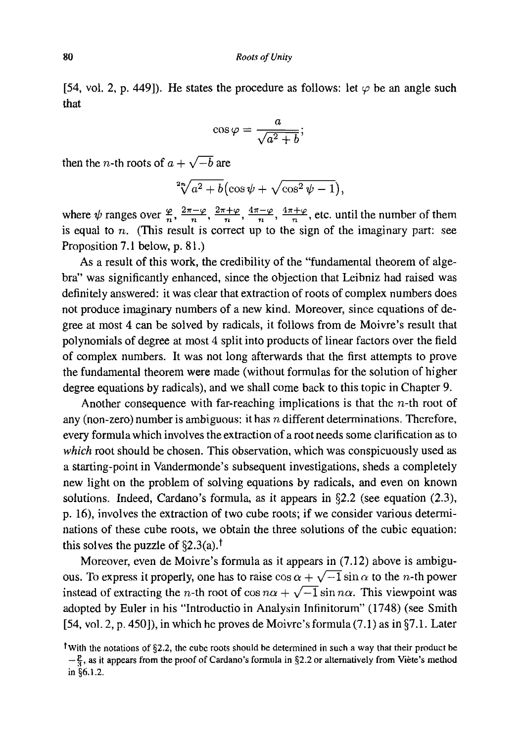
PROBLEMA MATHEMATICVM
MMiial I Kim i>t:t Mjlbimtlicu *d co-jhuimdi prcpcfilum,
SI dtiorumtcrminorum priorisad poftciiorcm pvo-
portiofir, uc i_ Q ad 45 G)_-- 3-5,5 (J) + ?) 5634
(D -" "}> 8)o(Mi) + "8|> '37J (9.) - 3451» i°7J © +
1,0530, ÓC75 (k) -- 2,3167, ói8o (ií) + 3, 8494,2375
J¡2) -- 4,8849, 411J A9) ^4,8^4,1800 {z7)-- 3,7865,
ÍSS00 (:\) + 2,3003,0651 (ir) —1,1767,9100 A7) + 4695,
5700 (I») - 1494,5040 (TJ) 4^376,4565^)- 74.0259
(_H)_+ H..U50 (O) -- 1,1300 E!>) + 945 D¿) - 45 D?) +
1 D¿), decurque terminus poftcriorjinvciiircpriorcm.
Ext>nf./um priiK/tm datum.
f p
Sltterminnipofteriorriii». i + rtin.i +riin 2. |;
ptior.Soi.viio.Dico tcrminúpriorcm cilcriin. 2 ~rbin.x
ri»». 1 +r j.
ExempUm (icHndum d*tnm.
SitccrminDjpofteciot r(ii). 1 4* ?('■■ 1 - '(<*■ i - ríi». 1 - rhiti. i-r¡,
quzriiurtriminuiprior.Soi.VTio. Tcr/r.iniisptiorcft rí«>. 2 - r¿i*. 1 +
fc bi b
Exempímm tert'mm dttum.
Sitrermingspoíccrior riw. l + r *, quxritur terminus prior.
Sou Terminus prior eft r b%u. x-r ^Mddrin. i + rJ_+ r ^ + r f i». _!_- r J_
Si in numrris abfolotis folinoroiji id proponere/ibuerit: Sit portcrior tcrmi-
4l
I OQOO,OOOO.OOOO,0000.005O,OOOO,CQOO.OC OO.OC ^O.ODOO.ÜOOO^OO
Quarríturieirninusprur. Solvtio. Terminus prior erit
«SSSSl
i&v
v^?, 0^00,0000,0000,0000. oooo,oooo,3S 50,oooo(oooo.
EXZMFLVM QV.ÍSIIVM,
C Itpofteriorterminus r tr'momlt \ JL -- r -L — r ¿/«. 1JL — r *t:
J r +16 t o+.
quariturrcrminnsprior. Hocexemptum orrnibiii M.iih-t7iit«cisacicon-
ftnicndum (it propofittim. Nondnbiioquin Lfiilf vat) C;!ltr> e)iis iolu-
uoaeni.feltem in oumciis (bUncunijs fie invemuxus.
M E-
[48, p. **iijV°] (Copyright Bibliothcque Albert 1 er, Bruxelles, Reserve précieuse, cote VB4973ALP)
= \/3.414213562373095048801688724209698078569671875375,

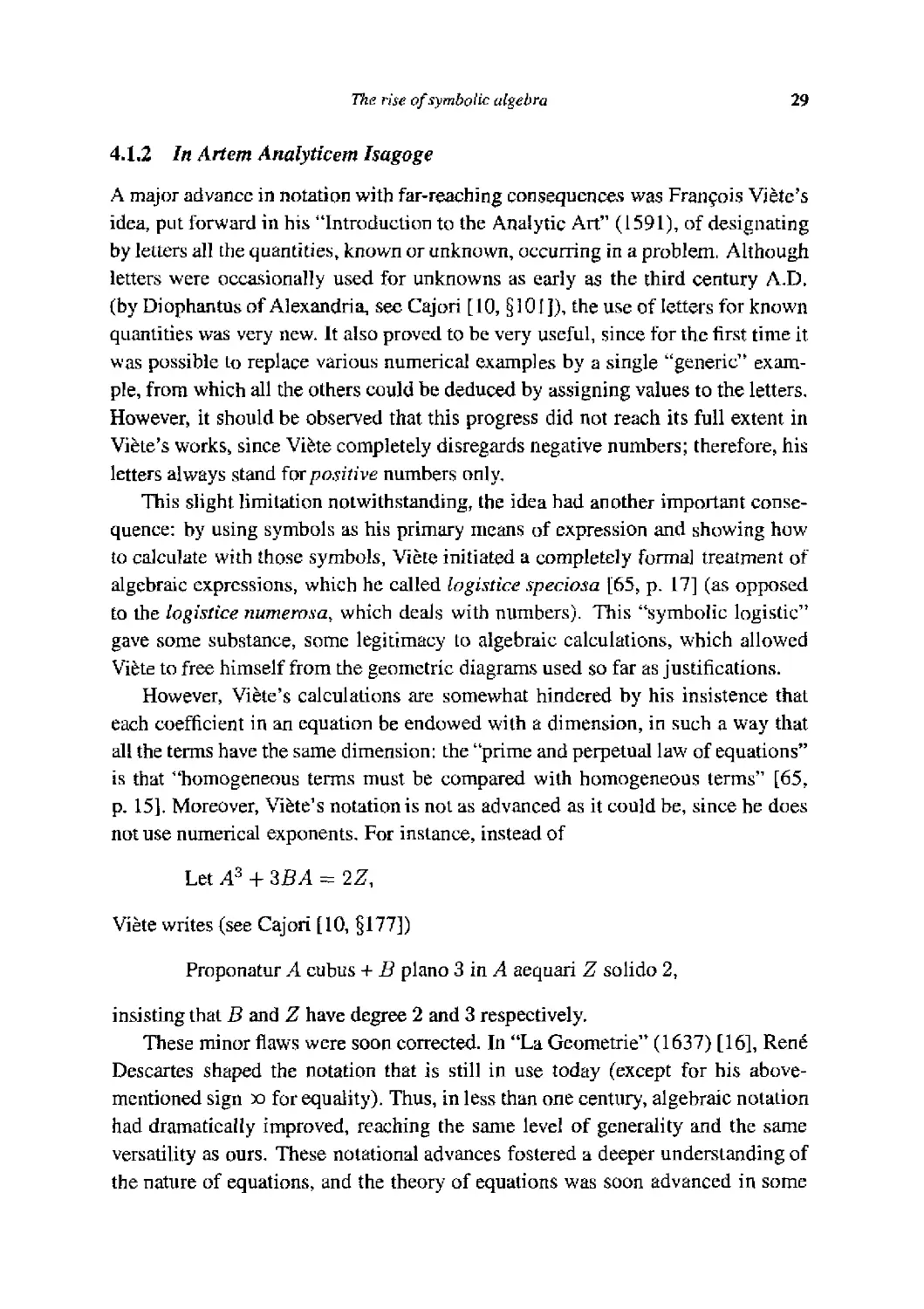
32 Hie Creation of Polynomials
then
X =
= ^0.0027409304908522524310158831211268388180,
and he asked for a solution when
Of course, this was not just any 45th degree equation; its coefficients had been
very carefully chosen.
When this problem was submitted to Viéte, he recognized that the left-hand
side of the equation is the polynomial by which 2 sin 45a is expressed as a func-
function of 2 sin a (see equation D.2) below, p. 33). Therefore, it suffices to find an
arc a such that 2 sin 45a = A, and the solution of Van Roomen's equation is
X = 2 sin a. In Van Roomen's examples:
(a) A = 2 sin ^f, and X =
(b) A should be 2 sin ^ff, and X = 2 sin ^,
(c)A = 2 sin ff, and X = 2sin ^r^,
and in the proposed problem A = 2 sin ^g, whence X = 2 sin ¡¿^i- That Van
Roomen's examples correspond to these arcs can be verified by the formulas
2 sin f = ±\/2-2cosa 2 cos f = ±v/2 + 2cosa
2 cos | = 1 2 sin f = V3
(see also remark 7.6). From these last results, the value of sin j^ an<^ °f cos fs
can be calculated by the addition formulas, since ^ = ^f — f •
It turns out that the solution 2 sin ^p- of Van Roomen's equation could also
be expressed by radicals, but this expression, which does not involve square roots
only, is of little use for the determination of its numerical value since it requires
the extraction of roots of complex numbers, see Remark 7.6, p. 85. Only the
numerical value, suitably approximated to the ninth place, is given by Viéte. But
Viéte does not stop there. While Van Roomen asked for the solution of his 45th
degree equation, Viéte shows that this equation has 23 positive solutions, and, in

Relations between roots and coefficients 33
passing, he points out that it also has 22 negative solutions [64, Cap. 6]. Indeed,
if a is an arc such that 1 sin 45a = A, then, letting
.2tt
afc=a+A-,
one also has 2 sin 45ak = A for all k = 0, 1,... , 44, so that 2 siller is a solution
of Van Roomen's equation. If A > 0 (and A < 2), then one can choose a between
Oand ^, whence
f> 0 forJfc = 0,... ,22,
2 sin Q> <
[<0 forfc = 23,... ,44.
Another interesting feature of Viete's brilliant solution [64] is that, instead of
solving directly Van Roomen's equation, which amounts, as we have seen, to the
division of an arc into 45 parts, Viéte decomposes the problem: since 45 = 32 ■ 5,
the problem can be solved by the trisection of the arc, followed by the trisection
of the resulting arc and the division into 5 parts of the arc thus obtained. As Viéte
shows, 2 sin 7ia is given as a function of 2 sin a by an equation of degree n, for n
odd (see equation D.2) below), whence the solutions of Van Roomen's equation
of degree 45 can be obtained by solving successively two equations of degree 3
and one equation of degree 5. This idea of solving an equation step by step was
to play a central role in Lagrange's and Gauss' investigations, two hundred years
later (see Chapters 10 and 12).
In modern language, Viéte's results on the division of arcs can be stated as
follows: for any integer n > 1, let [^j be the greatest integer which is less than
(or equal to) %, and define
If) f N
x
i=0 v
where (""') = ¿ZZ^ly. is the binomial coefficient. Then, for all n > 1,
2cosna = /riBcosa) D.1)
and for all odd n>l,
2sinna = (-l)(n-1)/2/nBsina). D.2)
Formula D.1) can be proved by induction on n, using
2cos(n + l)a = B cos a) B cos no) — 2cos(n — l)a

34 The Creation of Polynomials
and D.2) is easily deduced from D.1), by applying D.1) to fi — j — a, which
is such that cos,/? = sin a. (The original formulation is not quite so general, but
Viéte shows how to compute recursively the coefficients of /„, see ¡64, Cap. 9],
[65, pp. 432 ff] or Goldstine [27, §1.6].)
For each integer n > 1, the equation
MX) = A
has degree n, and the same arguments as for Van Roomen's equation show that
this equation has n solutions (at least when |j4| < 2). These examples, which are
quite explicit for n = 3,5,7 in Viéte's works [64, Cap. 9], [65, pp. 445 ft], may
have been influential in the progressive emergence of the idea that equations of
degree n have n roots, although this idea was still somewhat obscured by Viéte's
insistence on considering positive roots only (see also §6.1).
In later works, such as "De Recognitione Aequationum" (On Understanding
Equations), published posthumously in 1615, Viéte also stressed the importance
of understanding the structure of equations, meaning by this the relations between
roots and coefficients. However, the theoretical tools at his disposal were not
sufficiently developed, and he failed to grasp these relations in their full generality.
For example, he shows [65, pp. 210-211] that if an equation^
BPA -A3 = ZS D.3)
(in the indeterminate A) has two roots A and E, then assuming A > E, one has
Bp = A2 + E2
Zs = A2E + E2A.
The proof is as follows: since
BPA -A3 = ZS and BPE - E3 = Z\
one has BPA - A3 = B?E - E3, whence
Bp{A-E) = A3-E3
and, dividing both sides by A - E,
Bp = A2 + E2 + AE.
superscripts of B and Z indicate the dimensions: p is for piano and s for solido.

Relations between roots and coefficients 35
The formula for Zs is then obtained by substituting for Bp in the initial equation
D.3).
The structure of equations was eventually discovered in its proper generality
and its simplest form by Albert Girard A595-1632), and published in "Invention
nouvelle en 1'algebre" A629) [26].
As the next theorem needs new terms, the definitions will be
given first. [26, p. E2 v°]
Girard calls an equation incomplete it it lacks at least one term (i.e. if at least
one of the coefficients is zero); the various terms are called minglings ("meslés")
and the last is called the closure. The first faction of the solutions is their sum,
the second faction is the sum of their products two by two, the third is the sum of
their products three by three and the last is their product. Finally, an equation is in
the alternative order when the odd powers of the unknown are on one side of the
equality and the even powers on the other side, and when moreover the coefficient
of the highest power is 1.
Girard's main theorem is then [26, p. E4]
All the equations of algebra receive as many solutions as the
exponent of the highest quantity demonstrates, except the in-
incomplete ones: & the first faction of the solutions is equal to
the number of the first mingling, the second faction of the same
is equal to the number of the second mingling; the third to the
third, & so on, so that the last faction is equal to the closure, &
this according to the signs that can be observed in the alternative
order.
The restriction to complete equations is not easy to explain. Half a page later,
Girard points out that incomplete equations have not always as many solutions,
and that in this case some solutions are imaginary ("impossible" is Girard's own
word). However, it is clear that even complete equations may have imaginary
solutions (consider for instance x2 + x + 1 = 0), and this fact could not have
escaped Girard.
At any rate, Girard claims that the relations between roots and coefficients also
hold in this case, provided that the equation be completed by adding powers of the
unknown with coefficient 0. Therefore, the theorem asserts that each equation
Vn i o vn~2 i „ vn—A i „ vn~l i o vn—3 , „ vn—5 ,
A + S2-A + S4A + • ■ • = 8\A + S3A + SgA +••■

36 The Creation of Polynomials
or
Xn - SlXn-1 + s2l"-2 - s3Xn~3 + ■■■ + (-l)nsn = 0
has n roots xi,... ,xn such that
It should be observed that this "theorem" is not nearly as precise as the modern
formulation of the fundamental theorem of algebra, since Girard does not explic-
explicitly assert that the roots are of the form a + 6\/—T. It is therefore more a postulate
than a theorem: it claims the existence of "impossible" roots of polynomials, but
it is essentially improvable* since nothing else is said about these roots, except
(implicitly) that one can calculate with them as if they were numbers. Of course,
in all the examples, it turns out that the impossible roots are of the form a + 6-/—T,
but Girard nowhere explains what he has in mind.
One could say of what use are these solutions which are impos-
impossible, I answer for three things, for the certitude of the general
rule, & because there is no other solution, & for its utility. [26,
p.Fr°]
Girard elaborates as follows on the utility of impossible roots: if one seeks the
(positive) values of (x + IJ + 2, where x is such that x4 = Ax — 3, then since
the solutions of this last equation are 1, 1, —1 + >/—2 and -1 — y/-2, one gets
(x + IJ + 2 = 6, 6, 0 or 0, so that 6 is the unique result. One would never have
been so sure of that without the impossible roots.
Of course, Girard does not provide the faintest hint of a proof of his theorem.
It would have been very interesting to see at least how he found the relations
D.4) between the roots and the coefficients of an equation. These relations readily
follow from the identification of coefficients in
but this equality was probably not known to Girard. Indeed, Girard does not seem
to have been aware of the fact that a number a is a root of a polynomial P(X) if
* At least, the proof and, for that matter, even a correct statement of the theorem were very far beyond
the reach of seventeenth century mathematicians: see §9.2.

Relations between roots and coefficients 37
and only if X — a divides P(X): this observation is usually credited to Descartes
[16, p. 159], although Nunes may have been aware of it as early as 1567, and
perhaps earlier (see Bosnians [5, pp. 163 ff]).
On the subject of impossible roots, Descartes first seems more cautious than
Girard (the emphasis is mine):
Every equation can have as many distinct roots as the number of
dimensions of the unknown quantity in the equation. [16, p. 159]
This at least can be proved by Descartes' preceding observation (see theo-
theorem 5.15). However, Descartes further states:
Neither the true nor the false roots are always real; sometimes
they are imaginary; that is, while we can always conceive of
as many roots for each equation as I have already assigned, yet
there is not always a definite quantity corresponding to each root
so conceived of. [16, p. 175]
Around the middle of the seventeenth century, the fact that the number of so-
solutions of an equation is equal to the degree was becoming common knowledge,
like a piece of mathematical "folklore," accepted without proof and never ques-
questioned. At least, it was a good working hypothesis, and mathematicians started
to calculate formally with roots of equations without worrying about their nature,
pushing further Girard's results to discover what kind of information can be ob-
obtained rationally from the coefficients of an equation.
Girard himself had shown (omitting the details of his calculations) that the
sum of the squares of the solutions, the sum of their cubes, and the sum of their
fourth powers, can be calculated from the coefficients [26, p. F2 r°]: if x\,... ,xn
are the solutions of
Xn - SlXn'1 + S2Xn~2 - S3Xn-3 + ■■■ + (-l)nSn = 0,
let

38 The Creation of Polynomials
for any integer k; then
<J\ = Si,
IJ2 — s\ — 2S2;
cr3 = S
Around 1666, general formulas for the sum of any power of the solutions
were found by Isaac Newton A642-1727) [45, v. I, p. 519] (who was probably
unaware of Girard's work: see footnote A2) in [45, v. I, p. 518]). Newton's clever
observation is that, while the formulas for <j\, 02, ... in terms of si sn do
not seem to follow a simple pattern, yet there are simple formulas expressing a^
in terms of s\,... ,sn and a\,.., , <Jk-i- These formulas can be used to calculate
recursively the various a^ in terms of s\,... ,sn. Newton's formulas are
ÍT2 = SlO"! — 2S2,
(J3 = si<J2 - S2O1 + 3s3,
(J4 = S1ÍT3 - S2<T2 + S3CT1 - 4Si,
<r5 — S1ÍT4 — S2CT3 + ss<j2 - s4ai + 5s5,
and, generally,
íÜ^ÍÍ-l)^1^^-* + (-l)fc+1fc sk for k < n,
(Ju ^
These formulas (for k < n) were published without proof in "Arithmetica Uni-
versalis" A707) [46, p. 107] (see also [45, vol. I, p. 519; vol. V, p. 361]). Various
ingenious proofs have since been proposed (see for instance Bourbaki [6, App. 1
n° 3]); the following elementary proof is perhaps not very different from Newton's
own calculations.
For any integers a, b with 1 < a < n and b > 1, let r(a, b) be the sum of the
various different terms obtained from x\x2 ■ ■ ■ xa by permutation of x\,... , xn;
thus

Relaüons between mots and coefficients 39
and, for u, b > 2,
_(„ M - V V Th T- T-
Tl«J°J - ¿^ 2^ xil3;,2...xtcl.
¿1=1 *2<Í3<---<ía
Since, for b > 2, each term x¡ix¿2 ... xIa can be obtained as a product
the produet ¿>acrt,_i yields all the terms of r(a, £>); moreover, this produet also
yields terms like xj^ .. .xia+l, \fa<n—l. Furthermore, if b = 2, then each
of these latter terms is obtained {a + 1) times, while they are obtained only once
if b > 2. Therefore, we have the following results:
r(a, b) = sa<Ti,--¡ - t(<i. + 1,6-1) for a < n and b > 2, D.5)
t(c, 2) = san-\ - (a + l)«o+i for a < to, D.6)
r(n, íj) = snob_i for 6 > 2. D.7)
Since r(l, fc) = a^, equation D,5) with a—I and b — k yields
t-i — TB Jt — 1)
Equation D.5) with a = 2 and i> = k -1 can then be used to eliminate rB, fc - 1),
yielding
ffc = s-iOk-\ - s2Ok-2 + tC, fc - 2).
Next, we use D.5) with a = 3 and b = k — 2 to eliminate rC, fc — 2), and so on.
After a certain number of steps, we obtain
- S2ffc-2 H + (-l)fcr(fc -1,2) if fc < n,
whenee, using D.6),
<7fe = SlO-fc-l -S2O-fc-2H h (-l)feSfe_iG1+ (
If fc > to, we obtain
cffe = s^k-i - S2^fc-2 H h (-l)n+1r{n, fc + 1 - n)
whence, by D.7),
O-fe = Sifffc-! - S2Cfc-2 H h (-l)Tl+1Snt7A._n,
completing the proof.

40 The Creation of Polynomials
This, of course, was not Newton's most prominent achievement, even if we
consider only his contributions to the theory of equations. Indeed, Newton was
much more interested in numerical aspects (see for instance Goldstine [27, chap-
chapter 2]).
Numerical methods to find the roots of polynomial equations were at first one
of the several aims of the theory of equations, developed by some of the same
authors who developed other aspects: see for instance Cardano's "golden rule"
[11, ch. 30], Stevin's "Appendice algebraique" [55, pp. 740-745] or Viete's "De
numerosa Potestatum ad Exegesim Resolutione" (On the numerical resolution of
powers by exegetics) [65, pp. 311-370]. These numerical methods were much
more successful for the solution of explicit numerical equations than the algebraic
formulas "by radicals"; indeed, algebraic formulas are available only for degrees
up to 4 and they are by no means more accurate than the numerical methods (see
also §2.3). Therefore, the numerical solution of equations soon developed into
a new branch of mathematics, growing more accurate and powerful while the
algebraic theory of equations was progressively stalled.
Since the discussion of numerical methods falls beyond the scope of this book,
we take the occasion of this period of relatively low activity in algebra to justify
a pause in the historical exposition. We turn in the next chapter to a modern
exposition of the above-mentioned results on polynomials in one indeterminate,
in order to show on which mathematical base later results were grounded.

Chapter 5
A Modern Approach to Polynomials
5.1 Definitions
In modern terminology, a polynomial in one indeterminate with coefficients in a
ring A can be defined as a map
P: N^A
such that the set supp P = {n G N | Pn ^ 0}, called the support of P, is finite.
The addition of polynomials is the usual addition of maps,
(P + Q)n =Pn+Qn
and the product is the convolution product
(PQ)n = J2 P< ■ Qj-
i+j=n
Every element a e Ais identified with the polynomial a: N —» A which maps 0
to a and n to 0 for n ^ 0. Denoting by
X: N^A
the polynomial which maps 1 onto the unit element 1 G A and the other integers
to 0, it is then easily seen that every polynomial P can be uniquely written as
Therefore, we shall henceforth denote by
+ --- + anXn E.1)
41

42 A Modern Approach lo Polynomials
(as is usual!) the polynomial which maps j e N to o¡ for ¿ = 0 n and
to 0 for i > n. Accordingly, the set of all polynomials with coefficients in A
(or polynomials over A) is denoted A[X). Straightforward calculations show that
A[X] is a ring, which is commutative if and only if A is commutative.
The ring of polynomials in any number rn of indeterminatcs over A can be
similarly defined as the ring of maps from Nm to A with finite support, with the
convolution product.
Of course, the definition above is not quite natural. The naive approach to
polynomials is to consider expressions like E.1), where X is an undefined object,
called an indeterminate, or a variable. While this terminology will be retained in
the sequel, it should be observed that, without any other proper definition, to say
something is an indeterminate or a variable is hardly a definition. Moreover, it
fosters confusion between the polynomial
P(X) = a0 + aiX + ■ ■ ■ + anXn
and the associated polynomial function
P(-): A->A
which maps x £ A onto P(x) — oo + aix + • ■ ■ + anxn. This same confusion
has prompted the use of the term constant polynomials for the elements of A,
considered as polynomials. While this confusion is not so serious when A is a
field with infinitely many elements (see Corollary 5.16 below, p. 52), it could
be harmful when A is finite. For instance, if A = {oi,... , on} (with n > 2),
then the polynomial (X — a±) ■ ■ • (X — an) is not the zero polynomial since the
coefficient of Xn is 1, but its associated polynomial function maps every element
of A toO.
The degree of a non-zero polynomial P is the greatest integer n for which the
coefficient of Xn in the expression of P is not zero; this coefficient is called the
leading coefficient of P, and P is said to be monic if its leading coefficient is 1.
The degree of P is denoted by deg P. One also sets deg 0 = -oo, so that the
following relations hold without restriction if A is a domain (i.e. a ring in which
ab = 0 implies o = 0 or b = 0):
deg(P + Q) < max(degP, degQ),
deg(PQ) = deg P+deg Q.

Euclidean division 43
When A is a (commutative) field, the ring A[X] has a field of fractions A(X),
constructed as follows: the elements of A{X) are the equivalence classes of cou-
couples f/g, where /. g e A[X] and j^O, under the equivalence relation
r/g' if g'i = f'g.
The addition of equivalence classes is defined by
(/l/ffi) + U2/92) = (/1S2 + h9\)h\Q2
and the multiplication by
It is then easily verified that A(X) is a field, called the field of rational fractions in
one indeterminate X over the field A. The same construction can be applied to the
ring of polynomials in m indeterminates and yields the field of rational fractions
in m indeterminates over the field A.
However, the ring A\X] of polynomials in one indeterminate over a field A has
particularly nice properties, which follow from the Euclidean division algorithm.
These properties are reviewed in the next section.
5.2 Euclidean division
From now, we only consider polynomials over a field F.
5.1. Theorem (Euclidean Division Property). Let Pi, P2 e F[X]. If
P-2 ^ 0, then there exist polynomials Q, R e F[X] such that
P, = P2Q + R and deg R < deg P2.
Moreover, the polynomials Q and R are uniquely determined by these properties.
The polynomials Q and R are called respectively the quotient and the remain-
remainder of the division of Pi by P2.
Proof. The existence of Q and R is proved by induction on deg P1. If deg Pi <
degP2, we set Q = 0 and R = PY. If deg Pi - degP2 = d > 0, then letting
c € F be the quotient of the leading coefficient of Pi by that of P-2, we have

44 A Modern Approach to Polynomials
Therefore, by the induction hypothesis, there exist Q and R € F[X] such that
Pl-cXdP2 = P2Q + R and dcgi?<degP2.
This equation yields
Pi = PiiQ + r.Xd) + R
whence Q + cXd and R satisfy the required properties.
To prove the uniqueness of Q and R, assume
Pi = P2Q1 + Ri = P2Q2 + R2
with deg i?i < degP2 and deg R2 < degP2. Then fl, - R2 = P2{Q2 ~ Q\)
and this equality is impossible if both sides are non-zero, since the degree of the
right-hand side is then at least equal to deg P2, while the degree of the left-hand
side is strictly less than deg P2. Q
5.2. Definitions. Let Pu P2 e F[X]. We say P2 divides Pi if
P, = P2Q for some Q e F[X]
or, equivalently when P2 ^ 0, if the remainder of the division of Pi by P2 is 0.
A greatest common divisor (GCD) of Pi and P2 is a polynomial D 6 F[X]
which has the following two properties:
(a) D divides Px and P2,
(b) if 5 is a polynomial which divides Pi and P2 then 5 divides D.
If 1 is a GCD of Pi and P2, then Pi and P2 are said to be relatively prime.
Since it is by no means obvious that any two polynomials Pi, P2 have a GCD,
our first objective is to devise a method of finding such a GCD, thereby proving its
existence. We shall closely follow Euclid's algorithm for finding the GCD of two
integers or the greatest common measure of two line segments, assuming (without
loss of generality) that deg Pi > deg P2.
If P2 = 0, then Pi is a GCD of Pi and P2. Otherwise, we divide Pi by P2:
Pi=P2Qi + Ri- (E.I)
Next, we divide P2 by the remainder Ru provided that it is not zero,
Pi = R1Q2 + Ri (£.2)

Euclidean division 45
then we divide the first remainder by the second, and so on, as long as the remain-
remainders are not zero:
fíl
R,
Rn-2
= -H2Q3 +
— R
= R
= R
3Q4 +
n-lQn
nQn+l
R3
R4
+
+
Rn*
Rn+1-
(E
(£.3)
(EA)
(E.n)
.n + 1)
Since cleg P2 > deg R\ > deg R2 > .... this sequence of integers cannot
extend indefinitely. Therefore, Rn+i = 0 for some n.
Claim: If Rn+i = 0, then fin is a GCD of Pa and P2. (If n = 0, then set
To see that fin divides Pi and P2, observe that equation (E.n + 1), together
with Rn+i = 0, implies that iin divides fin-i- It then follows from equation
(E.n) that Rn also divides Rn-2- Going up in the sequence of equations (E.n),
(E.n - 1), (E.n - 2),... , (E.2), (E.I), we conclude recursively that Rn divides
ün_3, ■■- ,Ri,R\, P2andPi.
Assume next that Pi and P2 are both divisible by some polynomial S. Then
equation (E.I) shows that S also divides R±. Since it divides P2 and üi, 5 also
divides Ri, by equation (£.2). Going down in the above sequence of equations
(E.2), (E.3) (E.n), we finally see that S divides Rn. This completes the
proof that Rn is a GCD of P¡ and P2.
We next observe that the GCD of two polynomials is not unique (except over
the field with two elements), as the following theorem shows.
5.3. THEOREM. Any two polynomials Pj, P2 G F[X] which are not both zero
have a unique monic greatest common divisor DY, and a polynomial D G F[X]
is a greatest common divisor of Py and P2 if and only if D = cD\ for some
c, £ Fx (= F — {0}). Moreover, ifD is a greatest common divisor of Pi and P2,
then
D = Pit/i + P2U2 for some Ult U2 G F{X].
Proof. Euclid's algorithm already yields a greatest common divisor Rn of Pi and
P2. Dividing Rn by its leading coefficient, we get a monic GCD of Pi and P2.
Now, assume D and D' are GCDs of Pi and P2. Then D divides D' since D
satisfies condition (a) and D' satisfies condition (b). The same argument, with D

46 A Modern Approach to Polynomials
and D' interchanged, shows that D' divides D. Let D' = DQ and D = D'Q' for
some Q, Q1 £ F[X]. It follows that QQ' = 1, so that Q and Q' are constants,
which are inverse of each other. This proves at once the second statement and
the uniqueness of the monic GCD of Pi and P2, since D and D' cannot be both
monic unless Q = Q' = 1.
Suppose D is any GCD of Pi and P2; then D and the greatest common divisor
Rn found by Euclid's algorithm are related by D = cRn for some c € Fx.
Therefore, it suffices to prove the last statement for Rn. To this end, we consider
again the sequence of equations (E.I),... , (E.n). From equation (E.n), we get
Rn = Rn-2 — Rn-lQn-
We then use equation (E.n — 1) to eliminate Rn-i in this expression of Rn, and
we obtain
Rn = -Rn-zQn + Rn-2^ + Qn-lQn)-
This shows that ün is a sum of multiples of Rn-i and Rn~z- Now, Rn-i can
be eliminated using (E.n — 2). We thus obtain an expression of Rn as a sum of
multiples of .Rn_3 and ün_4. Going up in the sequence of equations (E.n — 3),
(E.n - 4),... , (E. 1), we end up with an expression of Rn as a sum of multiples
of Pi and P2,
Rn = P1U1+ P2U2
for some Uu U2 G F[X].
The argument above can be made more transparent with only a sprinkle of
matrix algebra. We may rewrite equation (E.I) in the form
(Qi l
P2 \ 1 0
equation (E.2) in the form
rj v i o; \r2
and so on, finishing with equation (E.n + 1) (with Rn+i = 0) in the form
Rn-A = (Qn+1 1\ (Rr,
Rn 1 0 0

Euclidean division 47
Combining the matrix equations above, we get
l l\ (Qi l\ (Qn
1 QJ\Q
Each matrix (^' ¿) is invertible, with inverse (J ^g;), hence the preceding
equation yields, after multiplying each side on the left successively by (° k ),
U -q2), ■•■ .
0 1 \ (Q 1 \ /0 1 \ /P
)\ )
If Ui, ... , UA G P[X] are such that
0 1 \ /0 1 WO 1
1 -Qn+J "A1 -Q2/ VI -Q
it follows that
U^Pi + U2P2 = Rn
(and U3Px + U4P2 = 0). D
Because of its repeated use in the sequel, the following special ease seems to
be worth pointing out explicitly:
5.4. COROLLARY. lfP\, P2 are relatively prime polynomials in F\X\, then there
exist polynomials V\, U-2 € F[X] such that
5.5. Remarks, (a) The proof given above is effective: Euclid's algorithm yields
a procedure for constructing the polynomials U1, U2 in Theorem 5.3 and Corol-
Corollary 5,4,
(b) Since the GCD of two polynomials Pi, P2 £ F[X] can be found by rational
calculations (i.e. calculations involving only the four basic operations of arith-
arithmetic), it does not depend on particular properties of the field F. The point of this
observation is that if the field F is embedded in a larger field K, then the poly-
polynomials Pj, iJ2 £ F[X] can be regarded as polynomials over K, but their monic
GCD in K[X] is the same as their monic GCD in P[^]. This is noteworthy in
view of the fact that the irreducible factors of Pi and P2 depend on the base field
F, as is clear from Example 5.7(b) below.

48 A Modem Approach to Polynomials
5.3 Irreducible polynomials
5.6. Definition. A polynomial F £ F[X] is said to be irreducible in F[X] (or
over F) if deg P > 0 and P is not divisible by any polynomial Q £ F[X] such
that 0 < deg Q < deg P.
From this definition, it follows that if a polynomial D divides an irreducible
polynomial P, then either D is a constant or degD = deg P. In the latter case,
the quotient of P by D is a constant, whence D is the product of P by a non-zero
constant. In particular, for any polynomial S e F[X], either 1 or P is a GCD of
P and S. Consequently, either P divides S or P is relatively prime to S.
5.7. Examples, (a) By definition, it is clear that every polynomial of degree 1 is
irreducible. It will be proved later that over the field of complex numbers, only
these polynomials are irreducible.
(b) Theorem 5.12 below (p. 51) will show that if a polynomial of degree at least
2 has a root in the base field, then it is not irreducible. The converse is true for
polynomials of degree 2 or 3; namely, if a polynomial of degree 2 or 3 has no root
in the base field, then it is irreducible over this field, see Corollary 5.13 (p. 51).
It follows that, for instance, the polynomial X2 — 2 is irreducible over Q, but not
over W. Thus, the irreducibility of polynomials of degree at least 2 depends on the
base field (compare Remark 5,5(b)).
(c) A polynomial (of degree at least 4) may be reducible over a field without
having any root in this field. For instance, in <Q[X], the polynomial X4 + 4 is
reducible since
X4 + 4 = (X'2 + 2X + 2)(X2 -2X + 2).
Remark. To determine whether a given polynomial with rational coefficients is
irreducible or not over <Q may be difficult, although a systematic procedure has
been devised by Kronecker, see Van der Waerden [61, §32]. This procedure is not
unlike that which is used to find the rational roots of polynomials with rational
coefficients, see §6.3.
5.8. THEOREM. Every non constant polynomial P € F[X] is a finite product
P = c ■ Pi ■ ... ■ P)V
where c E F* and P\, ..., Pn are monic irreducible polynomials {not neces-
necessarily distinct). Moreover, this factorization is unique, except for the order of the
factors.

Irreducible polynomials 49
Proof. The existence of the above factorization is easily proved by induction on
degP. If degP = 1 or, more generally, if P is irreducible, then P = c. ■ P\
where c is the leading coefficient of P and Pi = c^1 P is irreducible and monic.
If P is reducible, then it can be written as a product of two polynomials of de-
degree strictly less than deg P. By induction, each of these two polynomials has a
finite factorization as above, and these factorizations multiply up to a factorization
of P.
To prove that the factorization is unique, we shall use the following lemma:
5.9. Lemma. If a polynomial divides a product of r factors and is relatively
prime to the first r — 1 factors, then it divides the last one.
Proof. It suffices to consider the case r = 2, since the general case then easily
follows by induction.
Assume that a polynomial S divides a product T ■ U and is relatively prime to
T. By Corollary 5.4, p. 47, we can find polynomials V, W such that SV + TW =
1. Multiplying each side of this equality by U, we obtain
S(UV) + {TU)W = U.
Now, S divides the left-hand side, since it divides TU by hypothesis; it then fol-
follows that S divides U. □
End of the proof of Theorem 5.8. It remains to prove the uniqueness (up to the
order of factors) of factorizations. Assume
P = d\...Pn = dQ1...Qm E.2)
where c.,d € Fx and Pi,... , Pn, Qi, ■ ■ • , Qm are monic irreducible polynomi-
polynomials.
First, c — d since c and d are both equal to the leading coefficient of P.
Therefore, E.2) yields
I\...Pn = Ql...Qm. E.3)
Next, since Pi divides the product Q\... Qm, it follows from Lemma 5.9 that it
cannot be relatively prime to all the factors. Changing the numbering of Qi, • • ■ ,
Qm if necessary, we may assume that Pi is not relatively prime to Qi, so that
their monic GCD, which we denote by D, is not 1. Since D divides Pi? which is
irreducible, it is equal to Pi up to a constant factor. Since moreover D and Pi are
both monic, the constant factor is 1, whence D — P\.

50 A Modern Approach to Polynomials
We may argue similarly with Qi, since Qi is also monic and irreducible, and
we thus obtain D = Qi, whence
Pi = Qi-
Canceling Pi (= Q{) in equation E.3), we get a similar equality, with one factor
less on each side:
P2...Pn = Q2...Qm.
Using inductively the same argument, we get (changing the numbering of Q2,
... , Qm if necessary)
P2=Q2, P3=Q3, .-■ Pn=Qn,
and it follows that n < m. If n < m, then comparing the degrees of both sides of
E.3) we get
deg Qn+i = ■ ■ • = deg Qm = 0
and this is absurd since Qi is irreducible for i = 1, ,.. , m. Therefore, n — m
and the proof is complete. D
Lemma 5,9 has another consequence which is worth noting in view of its re-
repeated use in the sequel:
5.10. PROPOSITION. If a polynomial is divisible by pairwise relatively prime
polynomials, then it is divisible by their product.
Proof. Let Pi, ... , PT be pairwise relatively prime polynomials which divide a
polynomial P. We argue by induction on r, the case r = 1 being trivial. By the
induction hypothesis,
for some polynomial Q. Since Pr divides P, Lemma 5.9 shows that Pr divides
Q, so that Pi...Pr divides P. O
5.4 Roots
As in the preceding sections, F denotes a field. For any polynomial
P = a0 + aiX + ■ ■ ■ + anXn £ F[X)

Roots 51
we denote by P(-) the associated polynomial function
P(-): F^F
which maps any x e F to P(x) — a0 + aix + .,. + anxn. It is readily verified
that for any two polynomials P,Q € F[X] and any x 6 F,
(P + Q)(x) = P(x) + Q(x) and (P ■ Q)(x) = P(x) ■ Q(x).
Therefore, the map P i-> P(-) is a homomorphism from the ring F[X] to the ring
of functions from F to F.
5.11. Definition. An element a e F is a root of a polynomial P e F[X] if
5.12. THEOREM. An element a € F is a root of a polynomial P £
on/>> if(X - a) divides P.
Proof. Since deg(X - a) — 1, the remainder ¿Í of the division of P by (X — a) is
a constant polynomial. Evaluating at a the polynomial functions associated with
each side of the equation
P = (X-a)Q+R
we get
P{a) = (a - a)Q(a) + i?,
whence P{a) = R. This shows that P(a) — 0 if and only if the remainder of the
division of P by X — a is 0. The theorem follows, since the last condition means
that (X - a) divides P. D
5.13. COROLLARY. Let P E F[X] be a polynomial of degree 2 or 3. Then P is
irreducible over F if and only if it has no root in F.
Proof. This readily follows from the theorem, since the hypothesis on deg P im-
implies that if P is not irreducible, then it has a factor of degree 1, whence a factor
of the form X — a. O
5.14. Definitions. The multiplicity of a root a of a nonzero polynomial P is
the exponent of the highest power of X—a which divides P. Thus, the multiplicity
is m if (X - a)m divides P but (X - a)m+1 does not divide P. A root is called
simple when its multiplicity is 1; otherwise it is called multiple.

52 A Modern Approach to Polynomials
When the multiplicity of a as a root of P is considered as a function of P, it is
also called the valuation of P at a, and denoted va(P); we then set va(P) = 0 if
a is not a root of P. By convention, we also set va@) = oo, so that the following
relations hold for any P,Q G F[X] and any a e F
VaOP + Q) > min{Wo(P), uo(Q)), va(PQ) = va{P) + va(Q).
These properties are exactly the same as those of the function
-deg:
which maps any polynomial to the opposite of its degree, see p. 42. Accordingly,
(— deg) is sometimes considered as the valuation "at infinity."
5.15. THEOREM. Every non-zero polynomial P 6 F[X] has a finite number of
roots. If a\ ar are the various mots of P in F, with respective multiplicities
m\, ... , mr, then deg P > m\ + ... + mr and
for some polynomial Q E F[X] which has no root in F.
Proof. If «i, ... , ar are distinct roots of P in F, with respective multiplicities
nil, ■ ■ ■ i mr, then the polynomials (X — ai)mi, ... , (X — aT)mr are relatively
prime and divide P, whence Proposition 5.10 shows that
P = (X - ai)mi ---(X- ar)m'Qt
for some polynomial Q.
It readily follows that
deg P > mi + • ■ ■ + mr;
hence P cannot have infinitely many roots. The rest follows from the observation
that if ait... , ar are alt the roots of P in F, then Q has no root. d
5.16. Corollary. LetP,Q& F[X\. IfF is infinite, then P = Q ifandonly if
the associated polynomial functions P(-) and Q(-) are equal
Proof. If P(-) = Q(-), then all the elements in F are roots of P — Q, whence
P — Q = 0, since F is infinite. The converse is clear. D

Multiple roots and derivatives 53
5.5 Multiple roots and derivatives
The aim of this section is to derive a method of determining whether a polynomial
has multiple roots without actually finding the roots, and to reduce to 1 the multi-
multiplicity of the roots. (More precisely, the method yields, for any given polynomial
P, a polynomial Pg which has the same roots as P, each with multiplicity 1).
This method is due to Johann Hudde A633-1704). It uses the derivative of
polynomials, which was introduced purely algebraically by Hudde in his letter
"De Reductione Aequationum" (On the reduction of equations) A657) [31] and
subsequently applied to find maxima and minima of polynomials and rational frac-
fractions in his letter "De Maximis et Minimis" A658) [32].
5.17. Definition. The derivative dP of a polynomial P ~ a0 + axX -\ (-
anXn with coefficients in a field F is the polynomial
Straightforward calculations show that the following (familiar) relations hold:
Remark. The integers which appear in the coefficients of dP are regarded as el-
elements in F; thus, n stands for 1 + 1 + ■ ■ • + 1 (n terms), where 1 is the unit
element of F. This requires some caution, since it could happen that n = 0 in
F even if n ± 0 (as an integer). For instance, if F is the field with two elements
{0,1}, then 2 = 1 + 1 = 0 in F, whence non-constant polynomials like X2 + 1
have derivative zero over F.
5.18. LEMMA. Let a £ F be a root of a polynomial P E F[X]. Then a is a
multiple root ofP (i.e. va(P) > 2) if and only if a is a root ofdP.
Proof. Since a is a root of P, one has P = (X - a)Q for some Q £ F[X],
whence
dP = Q + (X - a)dQ.
This equality shows that X - a divides dP if and only if it divides Q. Since
this last condition amounts to (X - aJ divides P, i.e. va(P) > 2, the lemma
follows. □

54 A Modern Approach to Polynomials
5.19. PROPOSITION. Let P e F[X] be a polynomial which splits into a product
of linear factors* over some field K containing F. A necessary and sufficient
condition for the roots of P in K to be all simple is that P and dP be relatively
prime.
Proof. If some root a of P in K is not simple, then, by the preceding lemma, P
and dP have the common factor X — a in K[X\; therefore, they are not relatively
prime in K[X], whence also not relatively prime in F[X] (see Remark 5.5(b)).
Conversely, if P and dP are not relatively prime, they have in K[X\ a com-
common irreducible factor, which has degree 1 since all the irreducible factors of P
in K[X] are linear. We can thus find a polynomial X — a £ K[X] which divides
both P and DP, and it follows from the preceding lemma that a is a multiple root
ofPinK. D
To improve Lemma 5.18, we now assume that the characteristic of F is 0,
which means that every non-zero integer is non-zero in F. (The characteristic of
a field F is either 0 or the smallest integer n > 0 such that n = 0 in F).
5.20. PROPOSITION. Assume that charF = 0 and let a 6 F be a root of a
non-zero polynomial P € F[X]. Then
va(dP)=va(P)-l.
Proof. Let m = va(P) and let P = (X - a)mQ where Q e F[X] is not divisible
by X - a. Then
6P = {X- a)™-1 (mQ +{X- a)dQ),
and the hypothesis on the characteristic of F ensures that mQ ^ 0, Then, since
X — a does not divide Q, it does not divide mQ + {X — a)dQ either, whence
va(dP) = m-l. D
As an application of this result, we now derive Hudde's method to reduce
to 1 the multiplicity of the roots of a non-zero polynomial P over a field F of
characteristic zero. Let D be a GCD of P and dP, and let Ps = P/D.
5.21. THEOREM. Let K be an arbitrary field containing F. The roots of Ps
in K are the same as those of P, and every root of Ps in K is simple, i.e. has
multiplicity 1.
*In §9.2, it is proved that this condition holds for every (non constant) polynomial.

Multiple roots and derivatives 55
Proof. Since Ps is a quotient of P, it is clear that every root of Ps is a root of
P. Conversely, if a 6 K is a root of P, of multiplicity m, then the preceding
proposition shows that va(dP) = m — 1, and it follows that (X - aO™ is the
highest power of X — a which divides both P and dP. It is therefore the highest
power of X - a which divides D. Consequently, Ps is divisible by X — a but not
by (X — aJ, which means that a is a simple root of Ps. □
5.22. COROLLARY. IfP e F[X] is irreducible, then its roots in every field K
containing F are simple.
Proof. Since P is irreducible and does not divide dP, since deg dP = deg P — 1,
the constant polynomial 1 is a GCD of P and dP. Therefore, Ps = P and the
preceding theorem shows that every root of P in any field K containing F is
simple. D
This corollary does not hold if char F ^= 0. For instance, if char F = 1 and
a 6 F is not a square in F, then X2 — a is irreducible in F[X], but it has y/a as a
double root in F(-/a). (Observe that ->/a— -^/a since the characteristic is 2.)
5.23. Remarks, (a) Since a GCD of P and <9P can be calculated by Euclid's al-
algorithm (see p. 44), it is not necessary to find the roots of P in order to construct
the polynomial Ps. Thus, there is no serious restriction if we henceforth assume,
when trying to solve an equation P = 0, that all the roots of P in F or in any field
containing F are simple.
(b) In his work, Hudde does not explicitly introduce the derivative polynomial dP,
but indirectly he uses it. His formulation [31, Reg. 10, pp. 433 ff] is as follows :
to reduce to 1 the multiplicity of the roots of a polynomial
P = ao + axX + a2X2 -\ + anXn,
form a new polynomial Pi by multiplying the coefficients of P by the terms of an
arbitrary arithmetical progression m,m + r,m + 2r,... , rn + nr, so
Pi = aom + ai{m + r)X + a2(m + 2r)X2 H han(m +nr)Xn.
Then, the quotient of P by a greatest common divisor Di of P and Pi is the
required polynomial.
The relation between this rule and its modern translation is easy to see, since
Pi = mP + rXdP. Therefore, Di = D up to a non-zero constant factor, and
possibly to a factor X in £>1( if 0 is a root of P. So, Hudde's method yields the

56
A Modern Approach to Polynomials
same equation with simple roots as its modern equivalent, except that Hudde's
equation lacks the root 0 whenever 0 is a root of the initial equation.
5.6 Common roots of two polynomials
As the preceding discussion shows, it is sometimes useful to determine whether
two polynomials P, Q are relatively prime or not. The most straightforward
method is of course to calculate a GCD of P and Q, but there is another con-
construction, due to L. Euler A707-1783) (with different notations): the resultant of
P and Q. This construction is also basic for elimination theory; it will be used in
§§6.4 and 10.1.
Let
and
P = anXn
Q = bmXr
K * 0)
¿ 0)
be polynomials over a field F. The resultant of P and Q is the following
(m + n) x (m + n) determinant:
n-l
ax
a0
0
0
0
an
On-l
ax
a0
• r
0
m columns
0
0
an
an-\
a0
bm
bm-1
h
bo
0
•
0
o
bm
bm-1 ''■
h
b0 '••
0
n columns
0
0
bm
bm-1
h
bo

Common roots of two polynomials 57
5.24. THEOREM. Assume^ P and Q split into products of linear factors over
some field K containing F, and let R denote the resultant of P and Q. The
following conditions are then equivalent:
(a) P and Q are not relatively prime;
(b) P and Q have a common root in K;
(c) R = 0.
Proof (a) => (b) Let D be a GCD of P and Q. By hypothesis, D is not constant.
Moreover, since D divides P (and Q) which splits into linear factors over K, the
irreducible factors of D in K[X] have degree 1. Therefore, D has at least one root
in K, which is also a common root of P and Q since D divides P and Q.
(b) => (c) Let u 6 K be a common root of P and Q. Let
P=(X- u)Pi and Q = {X - u)Qx
where Pi, Qi £ K[X]. Then
PQi = QPi (=^-)- E-4)
From this equality, we obtain a system ofm + n equations by equating the coef-
coefficients of like terms. More precisely, if
P = anXn + an_1X"-1 + ■ ■ • + axX + a0,
Q = bmXm + bm-XXm~l + ■ ■ ■ + bxX + b0,
as above, and if
Pi = -(ziX"-1 + z2Xn-2 + ■■■+ zn^X + zn)
and
Qi - yiXm-x + y2Xm~2 + ■■■ + ym^X + ym,
then the coefficient of Xk in PQX -QiPis
arys+ ^ btzu
i-fj=fc r — s~k — m t—u~k — n
(where we set ar = 0 (resp. bt = 0) if r > n or r < 0 (resp. if í > mor
t < 0) and 2/s = 0 (resp. 2U = 0) if s > m or s < 1 (resp. u > n or u <
^Theorem 9.3, p. 116, will show that this hypothesis always holds.

58
A Modern Approach to Polynomials
1)), Therefore, equation E.4) is equivalent to the following system of equations,
whose left sides are the coefficients oiXn+m'\ Xn+m~2,... , Xn, Xn-\ ...,
X and the constant term in PQ\ — QP\.
+■
= 0
2 =0
= 0
= 0
+bozn= 0
E.5)
This system can be regarded as a system of m+n homogeneous linear equations in
theindeterminates y\,... , ym, zx,... , zn. It is easily verified that the coefficient
matrix of this system is the matrix which appears in the definition of R It follows
that R — 0, since t/j, ... , ym, z\, ... , zn is a non-trivial solution of this system.
(c) => (a) Assume now that R — 0; then, reversing the steps in the proof of
(b) => (c), we observe that the system E.5) has a non-trivial solution and conclude
that there exist non-zero polynomials Pj and Qi such that
AegP±<n-l, degQi<m-l.
(The inequalities deg Pi < n — 1 and deg Q\ < m■ — 1 occur when yi = z\ — 0.)
The preceding equality shows that P divides QP\. If P is relatively prime to Q,
then it divides Pj, by Lemma 5.9, p. 49. This is impossible since deg Pi < deg P;
therefore, P and Q are not relatively prime. D
Appendix: Decomposition of rational fractions in sums of
partial fractions
To find a primitive of a rational fraction § (where P, Q G R[X] and Q y¿ 0), it
is customary to decompose it as a sum of partial fractions in the following way.
factor Q into irreducible factors

Common roots of two polynomials 59
where Q\, ■ ■. ,Qr are distinct irreducible polynomials. Then there exist polyno-
polynomials Po, Pi,... , Pr such that
P = P+-i^ + +JL
and deg P¿ < deg Qf' for i = 1,... , r.
The existence of the polynomials Po, ... , Pr follows by induction on r from
the following proposition:
5.25. PROPOSITION. IfQ = SiS2 where Si and S2 are relatively prime polyno-
polynomials, then there exist polynomials Po, P\, P2 such that
Q~Po + Yi+Y2
and deg Pi < deg 5¿ for ¿ = 1,2.
Proof. Since Si and S2 are relatively prime, Corollary 5.4 (p. 47) yields
1 = S1T1 + S2T2
for some polynomials T\, T2- Multiplying each side by ^, we get
pIl PT<2
By Euclidean division of PT\ by S2 and of PT2 by ¿?i, we have
S2U2 + P2 and PT2 = 5, Ux +
for some polynomials U\, U2, Pi, P2 with deg P¿ < deg 5¿ for ¿ = 1,2. Substi-
Substituting for PTi and PT2 in the preceding equation, we obtain
Q S2 Si'
D
To facilitate integration, each partial fraction -£% (where Q is irreducible and
deg P < deg QTTl) can be decomposed further as
Q™ = ~Q + Q2 + " ' + Q™
with deg Pi < deg Q for i = 1, ... , m.

60 A Modern Approach to Polynomials
To obtain this decomposition, let Pi be the quotient of the Euclidean division
ofPbyQm-\
P=PlQm~1 +RX with degRx < deg Qm~J.
Since deg P < deg Qm it follows that deg P2 < deg Q. Let then P2 be the
quotient of the Euclidean division of R\ by Qm~2, and so on. Then
P = PxQm^ + P2Qm~2 + ■■■ + Pm_jQ + Pm, E.6)
and the required decomposition follows after the division of both sides by Qm.
Remark. The right-hand side of E.6) is the "Q-adic" expansion of P. When P
and Q are replaced by integers, equation E.6) shows that the integer P is written
as Pi Pa... Pm in the base Q.

Chapter 6
Alternative Methods for Cubic and Quartic
Equations
With their improved notations, mathematicians of the seventeenth century devised
new methods for solving cubic and quartic equations. The aim of this chapter is
to review some of these advances, in particular the important method proposed by
Ehrenfried Walter Tschirnhaus in 1683.
6.1 Viétc on cubic equations
Viéte's contribution to the theory of cubic equations is twofold: in "De Recogni-
tione Aequationum" he gave a trigonometric solution for the irreducible case and
in "De Emendatione Aequationum" a solution for the general case which requires
the extraction of only one cube root. These methods were both posthumously pub-
published in "De Aequationum Recognitione et Emendatione Tractatus Duo" A615)
("Two Treatises on the Understanding and Amendment of Equations," see [65]).
6.1.1 Trigonometric solution for the irreducible case
The irreducible case of cubic equations
X3+pX+q = 0
occurs when (|) + (§) < 0 (see § 2.3(c)). This inequality of course implies
p < 0, hence there is no loss of generality if the above equation is written as
X3 - 3a2X = a2b, F.1)
and the condition (|) +(|) <0 becomes a > 111. (Note that one can obviously
assume a > 0, since only a2 occurs in the given equation.)
61

62 Alternative Methods for Cubic and Quartic Equations
From the formula for the cosine of a sum of arcs (or from the general formula
D.1) in Chapter 4, p. 33), it follows that for all a G K
Ba cos aK - 3a2Bacosa) = 2aMcos3a.
Comparing with equation F.1), we see that if a is an arc such that
b
cos 3a = —,
2a
then 2a cos a is a solution of equation F.1). The two other solutions are easily
derived from this one; if ak = a + k~-, with ¿=1,2, then we also have
b
cos3afc = —,
¿a
whence the solutions of equation F.1) are
2a cos a,
2a cos (a + ~^j = —acosa — a\/3sina,
and 2acos(a + ^) = — acosa + av3sina.
Since Viéte systematically avoids negative numbers, he gives only the first
solution, which is positive if b > 0 (sec [65, p. 174]). However, he points out
immediately afterwards that a cos a + a\/3 sin a and a cos a — a\/3 sin a are so-
solutions of the equation
■)n2y y2 _ 1i
ou i — i — ci u.
This shows how clear was Viéte's notion of the number of roots of cubic equations,
6.1.2 Algebraic solution for the general case
Viéte suggested (in [65, p. 287]) an ingenious change of variable to solve the
equation
■q = 0. F.2)
Setting X = ^7 - Y and substituting in the equation above, he gets for Y the
equation

Viéte on cubic equations 63
whence Y3 can be found by solving a quadratic equation. The solutions are
Therefore, a solution of the cubic equation F.2) is given by
X--2- Y
X ~ 37 " Y'
where
2
Remarks, (a) If the other determination of 73 is chosen, namely
v'3 q
then the value of X does not change. Indeed, since (F7'K = - (|) , we have
and P
and sy
whence
P y_ P
37 3y
Incidentally, this remark also shows that Viéte's method yields the same result
as Cardano's formula, since after substituting for Y and Y' in the formula X =
-Y - Y', we obtain
(b) The case where 7 = 0 occurs only if p = 0; this case is therefore readily
solved.
(c) Viéte gives only one root, because in the original formulation the equation is*
A3 + WpA = 2Z3,
which has only one real root if Bv is positive, since the function A3 + ZBVA is
then monotonically increasing and therefore takes the value 2ZS only once.
*The exponents p, s are for piano and solido; unknowns are always designated by vowels.

64 Alternative Methods for Cubic and Quartic Equations
6.2 Descartes on quartic equations
New insights into the solution of equations arose from the arithmetic of polyno-
polynomials. In "La Geometric" Descartes recommends the following way of attacking
equations of any degree: "First, try to put the given equation into the form of an
equation of the same degree obtained by multiplying together two others, each of a
lower degree" [16, p. 192]. He himself shows how this method can be successfully
applied to quartic equations [16, pp. 180ff].
After canceling out the cubic term, as in Ferrari's method (Chapter 3), the
general quartic equation is set in the form
X4+PX2+qX + r = 0, F.3)
and we may assume q ^ 0, otherwise the equation is quadratic in X2 and is
therefore easily solved. We then determine a, b, c, d in such a way that
X4 + PX2 + qX + r = (X2 +aX + b)(X2 + cX + d).
Equating the coefficients of similar powers of X, we obtain from this equation
0 = a + c, F.4)
p = b + d + ac, F.5)
q — ad + be, F.6)
r = bd. F.7)
From equations F.4), F.5), F.6), the values of b, c and d are easily derived in
terms of a:
c = -a,
h —
u —
d =
a?
2
a2
T"
<P
h2
2
2a'
1
2a'
(Observe that a ^ 0 since q ^ 0.) Substituting for b and d in equation F.7), we
get the following equation for a:
a6 + 2pai + (p2 - 4r)a2 - q2 = 0. F.8)

Rational solutions for equations with rational coefficients 65
This is a cubic equation in a2, which can therefore be solved. If a is a solution of
this equation, then the given equation F.3) factors into two quadratic equations
whence the solutions are easily found.
6.3 Rational solutions for equations with rational coefficients
The rational solutions of equations with rational coefficients of arbitrary degree
can be found by a finite trial and error process. This seems to have been first
observed by Albert Girard [26, D.4 v°]; it also appears in "La Geometrie" [16,
p. 176].
Let
anXn + dn-il"-1 + • • • + aiX + a0 = 0 F.9)
be an equation with rational coefficients a¿ € <Q> for i = 0, ... , n. Multiplying
each side by a common multiple of the denominators of the coefficients if neces-
necessary, we may assume a¿ £ Z for i = 0, ... , n. Multiplying then each side by
a™~\ the equation becomes
(anX)n + on_1(onX)n-1 + an_2an(anX)n-2 + ■ • ■
2KX) + oooS = 0.
Letting Y — anX, we are then reduced to a monic equation with integral coeffi-
coefficients
Yn + bn^xYn-1 + bn_2Yn-2 + ■ ■ ■ + biY + b0 = 0 F4 € Z). F.10)
6.1. THEOREM. All the rational roots of a monic equation with integral coeffi-
coefficients are integers which divide the independent term.
Proof. Discarding the null roots and dividing the left-hand side of F.10) by a
suitable power of Y, we may assume bo ^ 0. Let then y € Q be a rational root of
F.10). Write y = ^ where j/i, y2 are relatively prime integers. From
yi\ \>-h fyi\
— )+o0 =

66 Alternative Methods for Cubic and Quartic Equations
it follows, after multiplication by y% and rearrangement of the terms,
1 2 + boy?)-
This equation shows that each prime factor of 1/2 divides y", whence also y\\
since yi and 1/2 are relatively prime, this is impossible unless yi has no prime
factor. Therefore yi = ±1 and y € Z.
To prove that y divides bo, consider again equation F.10) and separate off on
one side the constant term; we obtain
This equation shows that y divides b0, since the factor between brackets is an
integer. D
Tracing back through the transformations from equation F.9) to equation
F.10), we get the following result:
6.2. COROLLARY. Each rational solution of the equation with integral coeffi-
coefficients
anXn + an^iXn-1 + ■ • ■ + aiX + a0 = 0 (a¿ € 1)
has the form ya~n, where y €%isa divisor of
This last condition if very useful, in that it gives a bound on the number of
trials which are necessary to find a rational root of the proposed equation, provided
that ao t¿ 0. Of course, this can always be assumed, after dividing by a suitable
power of X.
For example, the theorem (or its corollary) shows that an equation like
Xn + a^-iX" + ■ • • + 01X ± 1 = 0
with ttj € % for i = 1,... , n — 1, has no rational root, except possibly +1 or —1.
"Other example, once very difficult" [26, E r°]: the rational solutions of
X3 = IX - 6
are among ±1, ±2, ±3, ±6. Trying successively the various possibilities, one
finds 1, 2 and -3 as solutions.

Tachimhaus' method 67
6.4 Tschirnhaus1 method
Although research on the theory of equations was not quite as active at the end of
the seventeenth century, substantial progress arose from a 4-page note by Tschirn-
Tschirnhaus [58], in 1683. This note proposes a uniform method to solve equations of
any degree.
The basic idea is very simple; it starts from the observation that it is always
possible to remove the second term of any equation
Xn + a,,.,!"-' + - • ■ + a,X + au = 0
by the simple change of variable Y = X + '-^-. (See e.g. §2.2 and §3.2). By
allowing more general changes of variable, such as
Y = Xm + i^-iX™-1 + ... + blX + bQt F.11)
Tschirnhaus aims to cancel out several terms of the proposed equation. More
precisely, by a suitable choice of the m parameters bo, E>i, ... , 6m_i, the above
change of variable yields an equation in y of the form
Yn + cn^1Yn'1 + ■ ■ ■ + ClY + co = 0
in which any m coefficients c¿ can be chosen to vanish. Roughly speaking, this
is because the m parameters bo, ... , bm-i provide m degrees of freedom, which
can be used to fulfill m conditions. In particular, taking m — n - 1, all the terms
except the first and the last could be removed, hence the equation in Y takes the
form
and is thus readily solved by radicals. Plugging in the solution Y — y/-c0 in
equation F.11), we then obtain a solution of the proposed equation of degree n
by solving an equation of degree m — n — 1, namely
Arguing by induction on the degree, it thus follows that equations of any degree
can be solved by radicals.
There is however a major obstacle, which was soon noticed by Leibniz [43,
p. 449, p. 403]: the conditions which ensure that all the coefficients c\, ... , cn_i
vanish yield a system of equations of various degrees in the parameters 6¿, and
this system is very difficult to solve. Indeed, solving this system actually amounts

68 Alternative Methods for Cubic and Quartic Equations
to solving a single equation of degree 1 • 2 - ... ■ (n — 1) = (n — 1)!. It thus
appears that this method does not work for n > 3, unless the resulting equation of
degree (n - 1)! has some particular features which make it reducible to equations
of degree less than n. This turns out to be the case for n = 4: the resulting sextic
can be seen to factor into a product of factors of degree 2 whose coefficients are
solutions of cubic equations (see Lagrange [40, Art. 41^4-5]), but for n > 5 no
such simplification is apparent. (Note that for composite n, Tschirnhaus' method
can be applied differently, and possibly more easily. For instance if n = 4, then
canceling out the coefficients of Y and Y3 reduces the equation in Y to a quadratic
equation in Y2.)
To discuss Tschirnhaus' method in some detail, we start by explaining how
the equation in Y can be found. This is a special instance of a general type of
problem which is dealt with by elimination theory. The problem is to eliminate
the indeterminate X between the two equations
Xn + a^iX"-1 + an_2Xn-2 + .-- + a1X + ao = 0, F.12)
Xm + bm^Xm-1 + bm^Xm~2 + --- + hX + bo = Y, F.13)
(with m < n), i.e. to find an equation R(Y) = 0, called a resulting equation,
which has the following properties:
(a) whenever x and y are such that equations F.12) and F.13) hold, then
R(y) - 0,
(b) whenever y is such that R(y) = 0, then equations F.12) and F.13) have
a common root x.
This last property shows that if R{Y) = 0 can be solved, then one (at least) of the
roots of equation F.12) is among the roots of equation F.13).
The properties of R(Y) can be rephrased as follows, considering F.12) and
F.13) as equations in X with coefficients in the field of rational fractions in Y:
R(Y) = 0 if and only if the polynomials
P(X) = Xn+ a».!!" +--- + a1X + a0
and
Q{X) ^Xm + bm^Xm~l + ... + blX + (ba-Y)
have a common root. As Theorem 5.24 (p. 56) shows, a solution of this problem

Tschimhaus' method
69
is the resultant* R(Y) of P and Q, defined as the determinant of the following
matrix:
/ 1
o
1
O a0
O
O 1 O
': bm-i 1
0 \ bm-l
1 t>l '.
*-i bo-Y h
0 60 -Y
0 a0
0 \
0
1
6m-l
b1
0 60 -y
m columns
n columns
Since the indeterminate Y appears only in the last n columns, it is easily veri-
verified that R is a polynomial of degree n in Y. Moreover, since the determinant is an
alternating sum of products of entries from different rows and columns, it follows
that products of only k factors 6¿ occur in the coefficient of Yn~k. Therefore,
R(Y) =
" + Cn-i
+ • • • + ClY +
where Cn_¿ is a polynomial of degree k in bo,... ,6m_i. (Actually,^ = (—1)".)
In order to cancel out Cn_l7 Cn_2, .... c\, consider now m = n - 1. The
preceding discussion shows that cn_i = Cn^2 = ■ ■ • = c\ = 0 is a system of
n - 1 equations of degrees 1, 2, 3, ... , n — 1 in the variables bQ &n-2-
Between these equations, n — 2 variables can be eliminated, and the resulting
equation in a single variable has degree 1 • 2 • 3 • ... ■ (n — 1) = (n — 1)! (see
for instance Weber [67, §53]). This was proved only much later by Bezout, but
by considering some examples one soon realizes that the solution of the above
system of equations is far from easy.
t It is slightly anachronistic to resort to determinants in this context, since they came into use somewhat
later, but the actual calculations in elimination theory were equivalent and they in fact motivated the
development of determinants.

70 Alternative Methods for Cubic and Quartic Equations
Let us consider for instance the cubic equation
X3+pX + q = 0 (p^O) F.14)
and let
Y = X2+b1X + b0. F.15)
Elimination of X between these two equations according to the method explained
above yields the following resulting equation in Y:
C3Y3 + c2Y2 + ClY + co = 0 F.16)
where
C3 = -1,
&i = 3bo — 2p,
c, = 4pb0 - 3qf>! - 36g - pb\ - p2,
co=q2 + p2b0 - pqbi + 3g60£>i - 2pb% + $- qb\ + pbQb2.
Thus, in order to cancel out C2 and c\, it suffices to let 60 = if and to choose for
61 a root of the quadratic equation
pb\ + 3qh - ~ = 0,
for instance
WIÍ+(!)-!)■
With the above choice of bo and 61, and letting A = \l(^) +(§) , we have
Therefore, a root of the resulting equation F.16) in Y is

Tschirnhaus' method 71
A root of the proposed cubic equation F.14) is then found by solving the quadrati c
equation F.15), which is now
F.17)
However, in general only one of the roots of this quadratic equation is a root of
the proposed cubic equation F.14). A better way to solve F.14) is to find the
common roots of F.14) and F.17), which are the roots of their greatest common
divisor.
Letting B = ^/A — \, one gets by Euclid's algorithm (p. 44) the following
greatest common divisor, if A ^ 0:
(It is easy to see that B2 + § 4- 0 if A ^ 0 and p ¿ 0.) There is thus only one
common root of F.14) and F.17); namely
Since B = {/-§ +y(|K + (|J, it is easily verified that
p J q j/P\3 , fí\2
= VVU +
thus the above formula for X is identical to Cardano's formula. (Compare also
Viéte's method in § 6.1.)
If A — 0, then the left-hand side of F.17) divides the given cubic polynomial,
so both roots of F.17) are roots of the proposed equation.

Chapter 7
Roots of Unity
7.1 Introduction
New branches of mathematics, such as analytic geometry and differential calculus,
came into being during the seventeenth century, and it is therefore not surprising
that investigations in the algebraic theory of equations came to a near standstill
at the end of this century, being pursued only occasionally by leading mathemati-
mathematicians such as Tschirnhaus. However, progress in other branches indirectly brought
some new advances in algebra. A case in point is the well-known "de Moivre's
formula": for every integer n and every a£l,
(cosa + ¿sina)" = cos(na) +isin(na), G.1)
which is easily proved by induction on n, since from the addition formulas for
sines and cosines it readily follows that
(cosa + ¿sina)(cos/3 + i sinC) — cos(a + 8) + isin(a + 0). G.2)
This formula G.1), and its proof through G.2), were first given by Euler in 1748
(see Smith [54, vol. 2, p. 450]) but it was already implicit in earlier works by
Cotes and by de Moivre. Actually, the above proof, simple as it is, is deceitful,
since it does not keep any record of the slow evolution which led to de Moivre's
formula. It is the purpose of this chapter to sketch this evolution and to discuss
the significance of de Moivre's formula for the algebraic theory of equations.
73

74 Roots of Unity
12 The origin of de Moivre's formula
While the differential calculus was being shaped by Leibniz and Newton, the in-
integration (or primitivation) of rational fractions was unavoidable. Very soon, for-
formulas equivalent to
ndx = for n ^ —1
and
dx
— = log i
X
became familiar, and the integration of any rational fraction in which the denom-
denominator is a power of a linear polynomial easily follows by a change of variable.
Moreover, around 1675, Leibniz had also obtained
from which the integration of other rational fractions can be derived.
The integration of rational fractions is the main theme of a 1702 paper by
Leibniz in the Acta Eruditoram of Leipzig : "Specimen novum Analyseos pro
Scientia infiniti circa Summas et Quadraturas" ("New specimen of the Analysis
for the Science of the infinite about Sums and Quadratures" [42, n° 24]). In this
paper, Leibniz points out the usefulness of the decomposition of rational fractions
into sums of partial fractions (see the appendix to Chapter 5) to reduce the inte-
integration of rational fractions to the integration of ~ and ^^ or, in his words, to
the quadrature of the hyperbola or the circle. Since this decomposition requires
that the denominator be factored in a product of irreducible polynomials, he is
thus led to investigate the factorization of real polynomials, coining close to the
"fundamental theorem of algebra" according to which every real polynomial of
positive degree is a product of factors of degree 1 or 2 (see Chapter 9).
Now, this leads us to a question of utmost importance: whether
all the rational quadratures may be reduced to the quadrature
of the hyperbola and of the circle, which by our analysis above
amounts to the following: whether every algebraic equation or
real integral formula in which the indeterminate is rational can
be decomposed into simple or plane real factors [= real factors
of degree 1 or 2], [42, p. 359]

The origin of de Moivre 's formula 75
Leibniz then proposes the following counterexample: since
z4 + a4 = (x2 + a2V^
it follows that
i4 + a4 =
(x + a
Failing to observe that
-a
he draws the erroneous conclusion that no non-trivial combination of the four
factors above yields a real divisor of x4 + a4.
Therefore, J x¿£ai cannot be reduced to the squaring of the cir-
circle or the hyperbola by our analysis above, but founds a new
kind of its own. [42, p. 360]
Even without deeper considerations about complex numbers, Leibniz could
have avoided this mistake if he had observed that, by adding and subtracting
2a2x2, one gets*
= (a;2 + a2 + y/2ax){x2 + a2 - V2ax).
As it appears from [45, v. IV, pp. 205 ff], Newton had also tried his hand at the
same questions as early as 1676, and he had obtained this factorization of x4 + a4,
as well as factorizations of 1 ± xn for various values of the integer n, (see the
appendix), but in 1702 he presumably did not care enough about mathematics any
more to point out the mistake in Leibniz's paper, had he been aware of it.
Leibniz's argument was definitively refuted by Roger Cotes A682-1716), who
thoroughly investigated the factorization of the binomials an ± xn, obtaining the
"This was pointed out by N. Bernoulli in the Acta Eruditorum of 1719.

76
Roots of Unity
following formulas:
m-1
fc=O
m-l
fc=o
(a2 -
G-3)
x + x2), G.4)
-War2), G.5)
fl
2m+1
These formulas appear in a compilation of Cotes' papers entitled "Theoremata
turn Logoinetrica turn Trigonométrica Datarum Fluxionum Fluentes exhibentia,
per Methodum Mensurarum Ulterius extensam" A722) ("Theorems, some ]o-
gometric, some trigonometric, which yield the fluents of given fluxions by the
method of measures further developed" [15, pp. 113-114]), in a very elegant form:
to find the factors of ax ± z\ it is prescribed to divide a circle of radius a into 2Á
equal parts AB, BC, CD, DE, EF, etc. Let O be the center of the circle and let
P be a point on the radius O A, at a distance OP = x (< a) from O. Then
ax - xx = OAX - OPX -AP-CP-EP- etc., and
ax + xx = OAX + OPX = BP-DP-FP- etc.
B.

The origin of de Moivre '¡formula
77
Exempli gratia (i A (it j, dividatur circumfercntia io 10 partes
atqualcs. critque A?*CT* ET*G T xIiP = OAt - O <P * cx-
iítcntc T intracirculum: & 2? F x Ü P xFTxHT*KT — OA'S
+OP'. Similiter fi \ lit tf, divifa circumfcrcntia in n partes
agúales: eric A<P-*C<P*ET*G'P*l<Pv.L<P-=.OAt-O<P*\
exilíente y ¡otra circulum5 & BT*eD'PxFeP*H'PK
[15, p. 114] (Univ. Cath. Louvain, Centre general de Documentation)
To check that this formulation is equivalent to the previous one, it suffices to
observe that, on the figure below,
we have, by Pythagoras' theorem,
CP2 = PR2 + RC2.
Since
PR= OP -OR = x- acosa and RC = asina,
it follows that
Therefore,
CP = y/x2 - 2axcosa + a2.
CP ■ C'P = x2 - 2ax cos a + a2.
Cotes' formulas were given without justification, but a proof was eventually
supplied in 1730 by Abraham de Moivre A667-1754), who had already obtained

78 Roots of Unity
some interesting results on the division of the circle. In a 1707 paper entitled
"Aequationum quaerundam Potestatis tertiae, quintae, septimae, novae, &c supe-
riorum, ad infinitum usque pergendo, in terminis finitis, ad imstar Regularum pro
Cubicis quae vocantur, Cardani, Resolutio Analytica" ("The analytic solution in
finite terms of certain equations of the third, fifth, seventh, ninth and other higher
powers, by rules similar to those called Cardano 's for the cubics", see Smith [54,
vol. 2, pp. 441 ffj), he had observed that the equation
fn(X)=2a (nodd)
where /„ is the polynomial by which 2 cos na is expressed as a function of 2 cos a
(see equation D.1) in Chapter 4, p. 33), has the solution
X = \Ja+ Va2 -1 + V a - \¡ a2 - 1,
for any value of a, whatsoever. In particular, if a = cos na, it follows that
2cosa— y coa na + V— 1 sin na + yeos na — -^—isinna, G.7)
although this formula does not appear explicitly in de Moivre's paper of 1707.
De Moivre's basic observation was that the equation fn(X) = 2a can be
obtained by elimination of z between the two equations
1 - 2a2" + z2n = 0, G.8)
1 - Xz + z2 = 0. G.9)
Indeed, equation G.9) yields
l+z2 = Xz
and, squaring both sides of this equation, we get
1 + z4 = {X2 - 2)z2.
These last equations show that, for n = 1, 2,
l + z2n = fn(X)zn. G.10)
From these initial steps, it is easily verified by induction that equation G.10) holds
for every integer n, using the recurrence formula
= Xfn(X) - fn-l{X) G.11)

The origin of de Moivre'¡formula
79
(see §4.2). Comparing G.10) with G.8), we obtain fn{X) = 2a, Now, dividing
by z both sides of G.9), it follows that X — z + z~x, while G.8) yields
zn = a ± Va2 - 1.
We thus obtain several equivalent expressions for X:
X = \Ja + s/a2 - 1 +
or X
or
a + \/a2 -1
\
X = \la + V'a2 - 1 + y a - \/a2 - 1,
X = ( Y a — \J a2 — 1J + ya — y a? — 1,
or X = I y a — \ a? — 1 I + ( V a + \l a2 — 1 I
V v / V v /
The equivalence of these expressions is easily derived from the equation
(a + \/a2 - l)(a - yja2 - 1) = 1.
De Moivre repeatedly returned to these questions in the sequel, displaying formula
G.7) quite explicitly on p. 1 of his book "Miscellanea Analytica" A730) (see
Smith [54, vol. 2, p. 446]). It is noteworthy that for X = 2 cos a and a = cos 7ia,
the values of z obtained by solving equations G.8) and G.9) are
cos na ±
-1 sin na
and
so that
X_
~2
"V" O
— I — 1 =
1 = cos a ± \/— 1 sin a,
cos na:
— 1 sin na — cos a ± v — 1 sin a
G.12)
but this was never written out explicitly by de Moivre.
Nevertheless, de Moivre's approach turned out to be quite fruitful, since Cotes'
formulas can be easily proved by pushing the preceding calculations a little further
(see Exercise 1).
In 1739, de Moivre used the trigonometric representation of complex numbers
and presumably also his formula, which certainly was thoroughly familiar to him
by then, to extract the n-th root of the "impossible binomial a + i/-6" (see Smith

80 Roots of Unity
[54, vol. 2, p. 449]). He states the procedure as follows: let y> be an angle such
that
then the n-th roots of a + %/—£> are
2\/a2 + b(cosip + \/cos2 ip — l),
where V ranges over *, n r, ^ , nr, ^y, etc. until the number of them
is equal to n. (This result is correct up to the sign of the imaginary part: see
Proposition 7.1 below, p. 81.)
As a result of this work, the credibility of the "fundamental theorem of alge-
algebra" was significantly enhanced, since the objection that Leibniz had raised was
definitely answered: it was clear that extraction of roots of complex numbers does
not produce imaginary numbers of a new kind. Moreover, since equations of de-
degree at most 4 can be solved by radicals, it follows from de Moivre's result that
polynomials of degree at most 4 split into products of linear factors over the field
of complex numbers. It was not long afterwards that the first attempts to prove
the fundamental theorem were made (without formulas for the solution of higher
degree equations by radicals), and we shall come back to this topic in Chapter 9.
Another consequence with far-reaching implications is that the n-th root of
any (non-zero) number is ambiguous: it has n different determinations. Therefore,
every formula which involves the extraction of a root needs some clarification as to
which root should be chosen. This observation, which was conspicuously used as
a starting-point in Vandermonde's subsequent investigations, sheds a completely
new light on the problem of solving equations by radicals, and even on known
solutions. Indeed, Cardano's formula, as it appears in §2.2 (see equation B.3),
p. 16), involves the extraction of two cube roots; if we consider various determi-
determinations of these cube roots, we obtain the three solutions of the cubic equation:
this solves the puzzle of §2.3(a).t
Moreover, even de Moivre's formula as it appears in G.12) above is ambigu-
ambiguous. To express it properly, one has to raise cos a + %/—lsin a to the n-th power
instead of extracting the n-th root of cos na + \/—l sin na. This viewpoint was
adopted by Euler in his "Introductio in Analysin Infinitorum" A748) (see Smith
[54, vol.2, p. 450]), in which he proves de Moivre's formula G.1) as in §7.1. Later
i the notations of §2.2, the cube roots should be determined in such a way that their product be
— if, as it appears from the proof of Cardano's formula in §2.2 or alternatively from Viéte's method
in §6.1.2.

The roots of unity
81
in the same book, comparing the power series expansions of the exponential and
of the sine and cosine functions, Euler also states
_ cos a _ )
a relation from which de Moivre's formula readily follows. Of course, once de
Moivre's formula is established, the other major results of this section, and in
particular Cotes' formulas, can be seen as easy applications. We devote the next
section to a streamlined exposition of de Moivre's results on the roots of complex
numbers along these lines.
7.3 The roots of unity
Let a and b be real numbers, not both zero, and denote by Va2 + b2 the (real,
positive) square root of a2 + b2. Since
_
there is a unique angle ip such that 0 < ip < 2n,
a
cos f =
and simp —
We thus obtain the trigonometric expression of the complex number a + bi ^ 0,
namely
a + bi = v a2 + b2(cos <p + i sin ip).
7.1. PROPOSITION. For any positive integer n, then distinct n-th mots of a + bi
are
' aJ + o (cos f-1 sin
n
n
G-13)
fork-0 n - 1.
In this formula, Va2 + b2 is the unique real positive 2n-th root of a2 + b2.
Proof. De Moivre's formula G.1) yields
+ ¿sin
n
= y az + b z(cosip + ism<p),

82 Roots of Unity
so that each of the expressions G.13) is an n-th root of o + bi. Moreover, these
expressions are easily seen to be pairwise distinct for fc = 0 n — 1, since
for these values of k it is impossible that two among the angles <P+^kn differ by a
multiple of 2tt. D
7.2. Definition. A complex number £ is called an n-th root of unity, for some
integer n, if £n = 1.
The set of all n-th roots of unity is denoted by /¿n. Thus,
By the preceding proposition we have
f 2W./77 2/ctt . 2kn , 1
fxn = \ e2h1'" = cos h ¿sin \k = 0, ... , n - 1 \,
Inn )
hence
). G.14)
This formula can be used to produce a factorization of Xn -1 into real factors;
indeed, if k + I — n, then
2/cTT 2¿7T , . 2/cTT 2¿7T
cos = cos -—- and sin = — sin ,
n n n n
whence
(v 2kn . . 2fc7r\/ 2Í-K . . 2£n\
X — cos i sin a - cos i sin =
\ n n J \ n n I
X2 -2cosí
V n
Therefore, multiplying the corresponding pairs of factors in the right-hand side of
G.14), we obtain
n-l
Xn-l = (X-l)f[ (X2 - 2cos(^)a- + l) if nis odd,
fc=i
¥■-1
t _ /l}.k"TT\ \
if n is even.
^ \ n. j /
k=\

The roots of unity 83
Substituting a/x for X in these formulas and multiplying each side by i" to
clear denominators, we recover Cotes' formulas G.5) and G.6). Formulas G.3)
and G.4) can be similarly derived by considering n-th roots of -1 instead of n-th
roots of 1.
It should be observed that, in a rectangular coordinate system, the points
(cos ^,sin~) forfc = 0, 1,... , n-1, which represent the n-th roots unity in
the planar representation of C, are the vertices of a regular polygon with n sides:
they divide the unit circle into n equal parts. For this reason, the theory which
is concerned with n-th roots of unity or with the values of the cosine and sine
functions at ^M. for integers k, n, is called cyclotomy, meaning literally "division
of the circle" [into equal parts].
Likewise, the n-th roots of any non-zero complex number are represented in
the plane of complex numbers by the vertices of a regular n-gon, as Proposi-
Proposition 7.1 shows.
That the roots of 1 deserve special interest comes from the fact that, if an n-th
root u of some complex number v has been found, then the various determinations
of y/v are the products wu, where w runs over the set of n-th roots of unity. This
is easily seen from
(WU)" = LOnUn = 1 ■ UU = V
or, equivalently, from Proposition 7.1.
While the n-th roots of unity have been determined above by a trigonometric
expression, yet the problem of deciding whether these roots of unity have an ex-
expression by radicals has been untouched. We now turn to this problem, and prove,
after some ideas of de Moivre:
7.3. Theorem. Let n be a positive integer. If, for each prime factor p ofn, the
p-th roots of unity can be expressed by radicals, then the n-th roots of unity can
be expressed by radicals.
This theorem follows by induction from the following result:
7.4. LEMMA. Let r and s be positive integers. lf£,i, ...,£,- (resp. Tji, . . . , i¡s)
are the r-th roots of unity (resp. the s-th wots of unity), then the rs-th roots of
unity are of the form t;n/rfjfori = 1, ... , r and j = 1, ... , s.
Proof. From the factorization of Ys - 1, it follows by letting Y = Xr that

84 Roots of Unity
Therefore, the rs-th roots of unity are the r-th roots of the various r}j, for j — 1,
... ,s. D
Proof of Theorem 7.3. We argue by induction on the number of factors of n. If
n is a prime number, then there is nothing to prove. Assume then that n = rs
for some positive integers r, s ^ 1. Then the number of factors of r (resp. s) is
strictly less than the number of factors of n, whence, by induction, the r-th roots
of unity £i, ... , £r and the s-th roots of unity 771, ... , r¡s can be expressed by
radicals. Since the n-th roots of unity are of the form £¿ tffjj, these can also be
expressed by radicals. D
7.5. Remark. Of course, the expressions thus obtained are not necessarily the sim-
simplest ones or the most suitable for the actual calculation of these roots. For in-
instance, since the 4-th roots of unity are ±1 and ±\/—I, the 8-th roots of unity are
obtained as
±1, iV^l, iyv^and ±\J-<f^í,
while they can also be expressed as
±1, ±a/—I, ——7=— and :
since cos f = sin \ = -4-.
Moreover, the result of Lemma 7.4 can be improved when r and s are rela-
relatively prime: in this case, one of the determinations of ^ffj is an s-th root of unity
rjk, so that the rs-th roots of unity are the products of the form ^r)k (i = 1, . • ■ , r
and k = 1 s), see Remark 7.13 (p. 90) and Exercise 3.
Theorem 7.3 shows that, in order to find expressions by radicals for the n-th
roots of unity, for any integer n, it suffices to consider the case where n is prime.
Since the equation Xn — 1 = 0 has the obvious root X = 1, we may divide
Xn - 1 by X — 1, and the question reduces to the following problem: solve by
radicals the equation
A +A + ■ • • + A -t- J. — U, (l-i-))
for n prime. This equation is readily solved for n = 2 and 3: the roots are -1 for
n = 2, and ~1±/~^ for n = 3.
For n > 5, the following trick (due to de Moivre) is useful: after division by
X2^", the change of variable Y = X + X transforms equation G.15) into
an equation of degree r~- in Y. (This trick succeeds because in the polynomial

The roots of unity 85
G.15) the coefficients of the terms which are symmetric with respect to the middle
term are equal.) Thus, for n = 5, we first divide each side of
Xa + X3 + X2 + X + 1 = 0
by X2, and the change of variable Y — X-\-X~l transforms the resulting equation
X2 + X + 1 + X-1 + X-2 = 0 into
We thus find
and the values of X are obtained by solving X + X~x = y for the various values
of Y. Thus, the 5-th roots of unity (other than 1) are the roots of the equations
Xi-Z±+^X + l = 0 and
which are
i/5-l± \/-10-2v/5 J
and
4
Similarly, for n = 7, de Moivre's trick yields for Y (— X + X~y) the cubic
equation
Y"A + Y2 - 27 - 1 = 0
which can be solved by radicals; the 7-th roots of unity can therefore be expressed
by radicals.
However, for the next prime number, which is 11, de Moivre's trick yields an
equation of degree 5, for which no general formula by radicals is known. Solving
this equation was one of the greatest achievements of Vandermonde (see Chap-
Chapter 11).
7.6. Remarks, (a) Since the roots of equation G.15) are e2k7Ti/n for k = 1, ... ,
n—\, the roots of the equation in y (= X + X-1)are
C2 w + e-2W» = 2 cos — for k = 1, ... , ^—-.
n 2

86 Roots of Unity
Therefore, the calculations above yield expressions by radicals for 2 cos ^ and
2 cos 4f as the positive and the negative root of Y2 + Y — 1 = 0,
2n x/51 4tt
2 cos — = —-— and 2 cos — =
5 2 5
(b) From Theorem 7.3 and the results above, it follows that the 2 • 33 • 52-th roots
of unity can be expressed by radicals. Hence, sin ^^ can also be expressed by
radicals, since
7T
sin
33-52 2iy >■
This explains why Van Roomen was able to give a solution by radicals in his third
example, see §4.2.
7.4 Primitive roots and cyclotomic polynomials
In this section, we complete our discussion of the elementary aspects of the theory
of roots of unity by listing several results which are more or less straightforward
consequences of de Moivre's formula.* They are a natural outgrowth of the theory
developed so far, and became known during the second half of the eighteenth
century. The central notion is the following:
7.7. DEFINITIONS. The exponent of a root of unity (, is the smallest integer e > 0
such that £fi = 1. For instance, the exponent of 1 is 1 and the exponent of —1 is
2, although 1 is an n-th root of unity for every n and —1 is an n-th root of unity
for every even n.
The n-th roots of unity of exponent n are also called primitive n-th roots of
unity.
We aim to give a complete description of the primitive n-th roots of unity and
to show that these roots are indeed primitive, in the sense that the other n-th roots
of unity can be obtained as powers of any such root. A basic ingredient in the
proofs is the following number-theoretic proposition:
^More precisely, these results follow from the fact that the set ¡xn of n-th roots of unity is a finite
subgroup of the multiplicative group of complex numbers.

Primitive roots and cyclotomic polynomials 87
7,8. THEOREM. Let d be the (positive) greatest common divisor of two integers
ni, n% Then there exist integers mi, m,2 such that
d — r¿i7r¡i +
In particular, ifrii and 712 are relatively prime, then there exist integers m^, m<i
such that
n\rt\\ + «27712 = 1.
Proof. Duplicate the arguments in the proof of Theorem 5.3 (p. 45) with integers
instead of polynomials. D
By the way, it is useful to note that most of the arguments in §§5.2 and 5.3
can be carried out with integers instead of polynomials, using the absolute value
of integers instead of the degree of polynomials; the point is that we also have a
Euclidean division property for integers: if m and n are integers and if m ^ 0,
then there are integers q, r such that
n = mq + r and 0 < r < \m\.
Moreover, the integers q and r are uniquely determined by these properties. Thus,
mimicking the proofs in §§5.2 and 5.3, we get a proof of the unique factorization
of integers into prime factors and obtain along the way other useful results like:
"If an integer divides a product of r factors and is relatively prime to the (r — 1)
first factors, then it divides the last one" (compare Lemma 5.9) or "If an integer is
divisible by pairwise relatively prime integers, then it is divisible by their product"
(compare Proposition 5.10).
Theorem 7.8 is sometimes known as "Bezout's theorem." This is clearly a mis-
misnomer, since it can be traced back at least to Bachet de Méziriac, in his "Problémes
plaisans et délectables qui se font par les nombres" A624). However, it could be
fair to associate the name of Bezout to a similar statement for polynomials with co-
coefficients in a field of rational fractions in one or several indeterminates (i.e. Theo-
Theorem 5.3 with F = K(Xl ,... , Xn) for some field K). This last result implies the
existence, for any two polynomials P\{Xi,... , Xn+i) and P^{Xi,.... Xn+1)
inn+1 indeterminates, of polynomials Qi{Xi,... ,Xn+i), Q2(Xi,... ,Xn+1)
and D{Xi,... , Xn) such that
P1Q1 + P2Q2 = D.

88 Roots of Unity
Since the indeterminate Xn+\ does not appear in D, one says that D is obtained
by elimination of Xn+i between Pi and P^. (The relation with the resultant of Pi
and P2 (considered as polynomials in Xn+1) is pointed out in Exercise 7.)
We now come back to roots of unity with the following result which charac-
characterizes the exponent of roots of unity:
7.9. LEMMA. Let e be the exponent of a root of unity C, and let m be an integer.
Then Qm = 1 if and only ife divides m. In particular, the exponent of an n-th mot
of unity divides n.
Proof. If e divides m, then m = ef for some integer /, and since £e = 1, it
readily follows from Cm = (Ce)f that Cm = 1-
Conversely, assume £m = 1 and let d be the greatest common divisor of m
and e. By Theorem 7.8, there are integers r and s such that
mr -f es = d.
Since Cd = (Cm)r(Os» we have (,d = 1; but since e is the smallest exponent for
which the power of £ is 1, it follows that d > e, whence d — e since d divides e.
Therefore, e divides m. D
7.10. Proposition. Let £ and r¡ be roots of unity of exponents e and f respec-
respectively. Ife and f are relatively prime, then £17 is a root of unity of exponent ef.
Proof. Since Cc = 1 and r\¡ = 1, we have
hence it follows from the preceding lemma that the exponent of £i?, which we
denote by k, divides ef.
On the other hand, from {(r})k = 1, it follows that
and raising each side to the power / yields
The preceding lemma then shows that e divides kf. Since e is relatively prime to
/, by hypothesis, it follows that e divides k. Likewise, interchanging C and ??> we
see that / divides k. Since e and / are relatively prime and divide k, their product
ef divides k; but we have already observed that k divides ef, hence k = ef. D

Primitive roots and cyciotomic polynomials 89
We now show that the primitive n-th roots of unity generate the other n-th.
roots of unity.
7.1 Í. PROPOSITION. ¡f'Q is a primitive n-th root of unity, then the n-th roots of
unity are of the form
Conversely, if C in an n-th root of unity such that every n-th root of unity is a power
of (, then C is primitive.
Proof. Since ( is an n-th root of unity, all the powers of ( are n-th roots of unity,
whence the set
consists of n-th roots of unity, i.e. S C ¡in. To prove that all the n-th roots of
unity are contained in S, i.e. S = ¡in, it then suffices to prove that S has n distinct
elements. This amounts to proving the following claim: the various powers C,1for
i = 0 n — 1 are pairwise distinct.
Assume on the contrary C = CJ for some i, j with 0<i < j <n — 1.
Then C,^~% — 1, whence, by Lemma 7.9, the exponent n of C divides j — i. This
is impossible, since 0 < j — i < n, and this contradiction proves the claim.
Conversely, assume that every n-th root of unity is a power of (. If £ is not
primitive, then (m = 1 for some positive integer rn < n. Then every power of
(, hence every n-th root of unity, is an m-th root of unity, i.e. ¡j,n C ¡¿m. This is
clearly impossible, since there are n distinct roots of unity while the number of
m-th roots of unity is only m. D
Remark. The proposition above shows that the (multiplicative) group /xn is gen-
generated by a single element: one says that ¡xn is a cyclic group. The proposition
also shows that the generators of \xn are the primitive n-th roots of unity.
A complete description of the primitive n-th roots of unity will be obtained as
a consequence of the following result:
7.12. Proposition. Let ( be a primitive n-th wot of unity and let k be an in-
integer. Then (k is a primitive n-th root of unity if and only ifk is relatively prime
to n,
Proof. Assume first that k and n have a common factor d ^ 1. Then

90 Roots of Unity
whence ((k)Tl/d — l since (n — 1. Therefore, the exponent of Cfc divides n/d,
hence (k is not a primitive n-ih root of unity.
Conversely, assume that Cfc is not primitive; then there is a positive integer
m < n such that (Cfc)m = 1. Since the exponent of ( is n, it follows from
Lemma 7.9 that n divides km. If n is relatively prime to k, then it divides m; but
this is impossible since m < n. Therefore, n and A; are not relatively prime. □
7.13. Remark. Let r and s be relatively prime integers and let 77 be a primitive
s-th root of unity. Proposition 7.12 shows that rf is a primitive s-th root of unity,
hence by Proposition 7.11 the s-th roots of unity are
Therefore, every s-th root of unity can be written as rf1 for some (unique) integer
i between 0 and s — 1, hence every s-th root of unity has an r-th root in ¡xs.
7.14. COROLLARY. The primitive n-th roots of unity are
2kir
f- I Sin
n n
where k runs over the positive integers which are less than n and relatively prime
to n. In particular, ifn is prime, then every n~th root of unity except 1 is primitive.
Proof. Let C = cos ^ + «sin ^. Since
r 2kir Ikix . , -1
Un = <, cos \- i sin k — 0,... , n — 1 V,
I n n i
we have by de Moivre's formula
Therefore, Proposition 7.11 shows that C, is a primitive u-th root of unity and it
follows from Proposition 7.12 that every primitive u-th root of unity is of the form
(k where A; is a positive integer relatively prime to n between 0 and ra — 1. D
We now introduce the polynomials which have as roots the primitive n-th roots
of unity. Because of their relation with the division of the circle, these polynomials
are called cyclotomicpolynomials.

Primitive roots and cyclolomic polynomials 91
7.15. Definition. The cyclotomic polynomials $„ (n = 1, 2, 3, ... ) are de-
defined inductively by 4>i (X) = X - 1 and, for n > 2,
Vn _ 1
where d runs over the set of divisors of n, with d ^ n.
In particular, if p is a prime number, we have
YP _ 1
*p(X) = -^r-- = X"-1 + Xp-2 + ■ ■ ■ + X + 1.
However, if n is not prime, it is not clear a priori that $„ is a polynomial. We
prove this and the fact that the roots of $n are the primitive n-th roots of unity
simultaneously:
7.16. Proposition. For every integer n > 1, the rational fraction $„ is a
monic polynomial with integral coefficients, and
c
where ( runs over the set of primitive n-th roots of unity.
Proof We argue by induction on n. Since the proposition is trivial for n = 1, we
assume that it holds for all integers up to n - 1. Then, for every divisor d of n,
with d t¿ n, we have
where £ runs over the roots of unity of exponent d. Since the roots of exponent d
are n-th roots of unity, it follows that <&d divides Xn — 1. Moreover, if d± and (¿2
are distinct divisors of n, then $di and <&d2 ^e relatively prime since their roots
are pairwise distinct. Therefore, by Proposition 5.10, the product Y\d $d{X) €
Z[X] divides Xn -1, and it follows that <&n(X) is a polynomial in Q[X], which is
monic since Xn — 1 and $d (for every proper divisor d of n) are monic. Moreover,
the proof of the Euclidean division property (Theorem 5.1, p. 43) shows that the
quotient of a polynomial in Z[X] by a monic polynomial in Z[X] is in Z[X].
Therefore, $n(X) E Z[X].

92 Roots of Unity
Now, the effect of dividing Xn - 1 by J] d\n ®d(X) is to remove from
all the factors X — C, where £ has exponent d ■£ n. Therefore, in &n(X) remain
all the factors X — ( where C has exponent n, and only those factors. Thus
where ( runs over the set of primitive n-th roots of unity. D
Remark It will be shown in Theorem 12.31 (p. 198) that $n is irreducible in
Q[-X], for every n. The proof is easier when n is prime, see Theorem 12.10
(p. 175).
Appendix: Leibniz and Newton on the summation of series
Around 1675, Leibniz obtained the following result, of which he was justifiably
proud:
1 111 7T
1 + 5-7+---=4-
His method was to use the formula
[-^-= tan'1 x, G.16)
which yields
í1 dx 7T
together with the power series expansion of (x2 + 1) \ namely
1
= 1 - x2 + x4 - x6 + x8
from which it follows that
/ —^ = / dx — / x2dx + I x4dx — • • •
Jo x2 + l Jo Jo Jo

Primitive roots and cyclolomic polynomials 93
Of course, the fact that the integral of the power series expansion of (x2 +1) *"l
is equal to the series of the integrals of the terms needs some justification, which
was supplied much later.
In 1676, Newton sent to Leibniz the following variant:
11111^1 n
3 5 7 9 11 13 15 2V2'
with the terse hint that it depended on the reduction of an integrand to partial
fractions (see [45, v. IV, p. 212]). It is very likely that Newton's result was obtained
from the evaluation of /0 xt+\ x ■ Indeed, the rational fraction ^d. has the
following decomposition into partial fractions:
x2 + 1 1 1 1 1
x4 + 1 2 X2 + V2X + 1 2 X2 - V2X + 1'
and, by the change of variable Y = \/2X + 1 (resp. Y = V2X - 1), it easily
follows from G.16) that
= V^tarT^v/^z+l),
x2 + V2x + 1
resp /
sp. /
J x2 -
+ 1
Therefore,
+ tan-^^ - 1)),
and since (\/2 + l)(v/2 - 1) = 1, we have
whence
r1 (x2 + l)dx 7T
x4 + l 2v^"
On the other hand, from the power series expansion
_1_ ARTO

94 Roots of Unity
it follows that
whence
/ 7 ! '-, / ^x ~r / x dx —IX ax —Ix ax + • • ■
JO x + L Jo Jo Jo Jo
1 l 1
This proves Newton's result.
Exercises
1. The aim of this first exercise is to prove Cotes' formulas along the lines of de
Moivre's calculations with polynomials (§7.2). Denote by fn{X) G Q[X] the
monic polynomial of degree n such that fnBcosa) = 2cosna (see equation
D.1) in Chapter 4, p. 33) and let, forn = 1, 2, 3,... ,
Pn(X, z) = l- fn(X)zn + z2n 6 Q[X, z].
(a) Prove: Pi(X,z) divides Pn(X,z) in Q[X, z] for every n. [Hint: Use
induction on n and the recurrence relation G.11), p. 78.]
(b) Prove: Pn{2 cos a,z)= Y[lZ_l Pi B cos (a + 2M), z) for a£l. [Hint:
Prove it first for a & fLZ, using (a) and observing that for a g ~Z the
polynomials in the right hand side are pairwisc relatively prime. Since the
coefficients of each side are continuous functions of a which are equal
outside a discrete subset of tt, they are equal for every a G K.J
(c) Show that for a — 0 both sides of the relation in (b) are squares. Extract-
Extracting the square root of each side, show that
and

Primitive mots and cyclotomic polynom ials 95
For q = ^, derive similarly the formulas
m— 1 / r* t -t \
and
m-l
Cotes' formulas G.3)-G.6) (p. 76) follow by substituting | for z and
multiplying each side by an appropriate power of a to clear denominators.
2. The following exercise aims to show some of the remarkable properties of the
polynomials fn of Exercise 1.
(a) Prove: fn(X) - 2 cos na = Uk^o{X - 2 cos (a + ^)) for a G M.
[Hint: Argue as in Exercise l(b).]
(b) Prove: fm(fn(X)) = fmn(X) for all integers m, n. [Hint: Use (a).]
(c) Prove: fm{X) • fn(X) = fm+n{X) + f\m-n\{X) for all integers m, n.
(To allow m — n, set/u(X) = 2,) [Hint: Use induction on n. Forn = 1,
use the recurrence relation G.11).J
3. Let fir = {£i,... , £r} and fi3 = {i]i,... , rja}. Assuming that r and s are
relatively prime, show that
Mrs = {&% | i = 1,... ,i-andj = 1,... ,s}.
[Hint: It suffices to prove that the products £¿tj¿ are pairwise distinct. Use Theo-
Theorem 7.8.]
4. Let (, be a root of unity of exponent e and let fc be an integer. Find the exponent
of (k. (Compare Proposition 7.12.)
5. Show that an n-th root of unity ( is primitive if and only if Cd 7^ 1 for every
proper factor d of n.
6. Let p be a prime number. Prove that
Ei _ / ° if ¿ £ Z is not divisible by p,
we \p if i e Z is divisible by p.
[Hint: Use Newton's formulas of Chapter 4.j

96 Roots of Unity
7. Let P = anXn+an-iXn~1 + - ■ -+aiX+a0 andQ = bmXnt+bm-1Xm-i +
■ • ■ + b\X + bo (with an, bm ^ 0) be polynomials over a field F, and let A be
the square matrix of order m + n which appears in the definition of the resultant
R of P and Q (so that R = det A, see §5.6, p. 56). Verify the following matrix
multiplication:
(Xm-!p ■■■ XP P Xn-XQ ■•■ XQ Q).
Multiply each side of this matrix equation by the transpose of the matrix of co-
factors of A. Considering the last entry of the resulting line matrices, conclude
that R is a linear combination of Xm~1P, ... , XP, P, Xn~lQ, .... XQ, Q,
hence that there exist polynomials {/, V 6 F[X] such that degi/ < m — 1,
deg V < n - 1 and
Using this result, give an alternative proof of Theorem 5.24.
8. This last exercise is an introduction to Euler's "totient function" (p. For any
integer n > 2, let <p(n) be the number of integers which are relatively prime to n
between Oandn- 1.
(a) Show that <p(ri) = deg $„ and that <p(n) is equal to the number of prim-
primitive n-th roots of unity.
(b) Show that <p(mn) = <p(m)<p(n) if m and n are relatively prime. [Hint:
Compare Exercise 3.]
(c) Show that f{pk) = pk~1(p - 1) for any prime number p,
(d) Derive from (b) and (c) the following formula: if n = pj1 • • • p$r (pi,
... , pr distinct prime numbers), then
(e) Show that n = Y^d\n ^(^) where d runs over the factors of n (including
n). [Hint: Compare Definition 7.15.]

Chapter 8
Symmetric Functions
8.1 Introduction
During the first half of the eighteenth century, the structure of equations, as for-
formerly investigated by Viete (§4.2), became clearer and clearer. Calculating for-
formally with roots of equations, mathematicians became aware of the kind of infor-
information that can be gathered from the coefficients without solving equations. As
Girard had shown (§4.2), for any polynomial
Xn - SlXn~l
we have
>xn
Si = 2
S2 = 2
s3 = a
— • • •
:i + ••
'l%2 +
;ix2x3
+ (-l)nsn =
(X-xl)(X-x2)--
+ i" Xn_2lTi-l3;ní
•(X
- Xn)
(8.1)
(8.2)
Sn =
The following question naturally arises: what kind of function of the roots xi,
... ,xn can be calculated from s\,... , snl
To translate properly the results of this period, laying on firm ground the for-
formal calculations with roots of polynomials, the roots xi,... ,xn should be consid-
considered as independent indeterminates over some base field F (usually, F = Q, the
field of rational numbers). Indeed, every calculation with indeterminates which
does not involve divisions by non-constant polynomials can be done as well with
97

98 Symmetric Functions
arbitrary elements in a field K containing the base field F. This is a loose transla-
translation of the fact that any map from {x\,... , xn} to K can be (uniquely) extended
to a ring homomorphism from the ring of polynomials F\xi,,., , xn] to K, map-
mapping a polynomial P(xi,... , xn) to the element of K obtained by substituting
forxi, ... ,xn their assigned values in K. (If we wish to allow divisions by non-
constant polynomials, caution is necessary since some denominators may vanish
in K.) Therefore, we introduce the following definition:
8.1. DEFINITION. If xi, .. . , xn are considered as independent indeterminates
over some base field F, the polynomial (8.1) above is called the general (or
generic) monic polynomial of degree n over F. Thus, this general polynomial
is a polynomial in one indeterminate X with coefficients in F[xi.... , zn]; it may
thus be viewed as an element in F[ii,... ,xn,X].
This polynomial is general (generic) in the following sense: if
P = Xn+ an_tXn-1 + an_2Xn-2 + --- + a1X + a0
is an arbitrary monic polynomial of degree n over some field K containing F,
which splits* into a product of linear factors in some field L containing K, so that
with u-i G L for i = 1,... , n, then there is a homomorphism F[x\.... , xn] —» L
mapping x¡ to u¿ for i = 1, ... , n. This ring homomorphism translates any
calculation with xi,... ,xn into a calculation with u\,... , un. For instance, it is
easily seen that this ring homomorphism maps si, s?,... , sn onto — ara_i, an-2,
... , (-l)noo € K, which means that
si(a;i,... ,xn) = -an_i, i.e. xi -\ r-xn = -on_i,
$2{xi,... ,!„) = an_2, i.e. xix2-\ ha:n_ixn =an_2,
sn(xi,... ,xn) = (~l)"a0, i.e. xi'-'Xn = (-l)"ao-
After this slight change of viewpoint, from arbitrary elements to indetermi-
indeterminates, the question becomes: which are the rational fractions in n indeterminates
*We shall see later that the condition that P splits into a product of linear factors in some field con-
containing K is always fulfilled, see §9.2. At this point this provision cannot be disposed of, however.
(Compare Remark 8.8(a) below, p. 105).

Introduction 99
x\, ... , xn that can be expressed as rational fractions in si, ... , sn (where si,
... , sn are defined by the equalities (8.2) above)?
The crucial condition turns out to be the following:
8.2. Definition. A polynomial P{x\,... , xn) in n indeterminates is symmet-
symmetric if it is not altered when the indeterminates are arbitrarily permuted among
themselves; i.e., for every permutation u of 1, ... , n,
P{xa(l),..., xa{n)) = P(xi,..., xn).
Similarly, a rational fraction 5 in n indeterminates is symmetric if it is not altered
when the indeterminates are permuted; i.e., for every permutation u of 1,... ,n,
P(xa{l),... ,xa{n)) =
Note that this does not imply that P and Q are both symmetric, since P and Q
can be both multiplied by an arbitrary non-zero polynomial without changing the
fraction §, but we shall see below (p. 104) that every symmetric rational fraction
can be represented as a quotient of symmetric polynomials.
Since the polynomials si,... , sn are symmetric, it is clear that every rational
fraction in si,... , sn is a symmetric rational fraction in xi,... ,xn. The converse
turns out to be also true, so that the following result holds:
8.3. THEOREM. A rational fraction in n indeterminates x\, ... , xn over afield
F can be expressed as a rational fraction in s\, ... , sn if and only if it is symmet-
symmetric.
This theorem is in fact a consequence of the analogous result for polynomials:
8.4. THEOREM. A polynomial in n indeterminates x\, ... ,xn over afield F can
be expressed as a polynomial in S\ sn if and only if it is symmetric.
These theorems are known as the fundamental theorems of symmetric frac-
fractions or symmetric polynomials respectively. The polynomials s\, ... , sn are
sometimes called the elementary symmetric polynomials, since the others can be
expressed in terms of these ones.
Because of their progressive emergence through the calculations of eighteenth
century mathematicians, these theorems can hardly be credited to any specific au-
author. (There is not much credit to give anyway, since the proofs are not difficult.)

100 Symmetric Functions
It seems that they first appeared in print around 1770, in "Meditationes Alge-
braicae" of Edward Waring A736-1798) and in "Mémoire sur la resolution des
equations" of A.T. Vandermonde, and in presumably other works. It is noteworthy
that Lagrange in 1770 qualifies the fundamental theorem of symmetric fractions
as "self-evident" [40, Art. 98, p. 372].
Therefore, the most interesting feature that one may expect of a proof is its
effectiveness: it has to provide a method to express any symmetric polynomial as
a polynomial in s\,... , sn. In the next section, we explain the particularly simple
method suggested by Waring [66, Chapter I, Problem III, Case 3], and thereafter
we shall discuss some applications, but first we point out a convenient notation
which allows to denote symmetric polynomials without writing out all the terms.
NOTATION. We let £ x^x^ ■ ■ • x)? be the symmetric polynomial whose terms
are the various distinct monomials obtained from x'^x'J ■ ■ -x1^ by permutation
of the indeterminates. Observe that this notation is slightly ambiguous, since the
total number of variables is not clear from the notation, as some of the exponents
i\, ... ,in may be zero. Therefore, the total number of variables should always
be indicated, unless it is clear from the context. For example, as a symmetric
polynomial in two variables,
whereas, as a symmetric polynomial in three variables,
£ x\x2 = x\x2 + xxx\ + x\xz + xxx\ + x%x3 + x2x\.
With this notation, the elementary symmetric polynomials can be written sim-
simply as
and sn = 1£lx1---xn (=xi---xn).
8.2 Waring's method
In order to define the degree of a polynomial in n indeterminates, we endow the set
N™ of n-tuples of integers with the lexicographic ordering. Thus (¿1,... ,in) >
(ii, • • • , Jn) if the first non-zero difference (if any) in the sequence i\ - ji,... ,
in - jn is positive. For any non-zero polynomial P = P(xi,... , xn) in n inde-
indeterminates Xi,... ,xn over a field, the degree of P is then defined as the largest

Waring's method 101
n-tuple (¿i,... ,in) 6 N" for which the coefficient of x \x ■■■ x^ in P is non-zero.
The degree of P is denoted by deg P. For instance, we have
= A,0,0,... ,0),
degs2 = (l,l,0,...,0),
(8.3)
degsn_i = A,1,..., 1,0),
deg sn = A,1,..., 1,1).
By convention, we also set degO = — oo, and the same relations as for polynomi-
polynomials in one indeterminate hold, namely
deg(P + Q)< max(deg P, deg Q), (8.4)
deg(PQ) = deg P + deg Q. (8.5)
Proof of Theorem 8.4. Waring's method to express any symmetric polynomial
P(xi,... , xn) as a polynomial in s\, ... , sn is quite similar to Euclid's divi-
division algorithm (Theorem 5.1, p. 43). The idea is to match P with a polynomial
in si,... , sn which has the same degree as P. Adjusting the leading coefficient,
we can arrange that the degree of the difference be less than deg P, and we are
finished by induction on the degree.
Let P 6 F[xi,... , xn] be a non-zero symmetric polynomial, and let
We first observe that ¿i > ¿2 > • • • > in- Indeed, if we can find among the terms
of P a term like axl1 ■••xi¿ (with a ^ 0), then we can also find all the terms
obtained from this one by permutation of x\, ... , xn, since P is symmetric.
The degrees of these terms are the various n-tuples obtained from (¿i,... ,in)
by permutation of the entries, and the greatest among these n-tuples is the one in
which the entries are in not-increasing order.
We can therefore set
f _ il-»2 J2-Í3 *n-l-¿n in
/ — s1 s2 ■ • •sn_1 sn .
By (8.3) and (8.5), we have
deg/ = (¿j - ¿2) deg(s!) + {i2 - ¿3) deg(s2) + --- + in deg(sn)
= (¿j -¿2,0,... ,0) + (¿2 -Í3,h-Í3,0,-.. ,0) + ■ • ■ + {in,... ,in)

102 Symmetric Functions
Moreover, it is readily verified that the leading coefficient of /, which is the coef-
coefficient of xl1 ■ ■ ■ xl£, is 1, so that
/ = ij1 • • -xj," + (terms of lower degree).
Therefore, if a e F* is the leading coefficient of P, so that
P = axl1 ■ ■ ■ x%£ + (terms of lower degree),
then, letting Pi = P — af, we see that deg Pi < deg P. Moreover, Pi is sym-
symmetric (possibly zero), since P and / are symmetric. We can therefore apply the
same arguments to Pi, which has lower degree than P.
In Waring's words:
The first step of the solution is to find Sa x Rb~a x Qc~b x
Pd~c...; among these terms one particular product will be the
required sum, while the remaining terms must be identified by
the same method and then discarded. [66, p. 13]
To complete the proof, it remains to prove that the process above, by which
the degree of the initial symmetric polynomial has been reduced, terminates in a
finite number of steps. This readily follows from the following observation:
8.5. LEMMA. N™ satisfies the descending chain condition, i.e., it does not con-
contain any infinite strictly decreasing sequence of elements.
Proof. As the lemma is obvious if n = 1, we argue by induction on n. If
(¿11, ¿12, • • • , ¿In) > (¿21, ¿22; • • ■ , ¿2n) > • ■ • > (¿ml, ¿m2, ■ • • j i-mn)
(8.6)
is an infinite strictly decreasing sequence in N", then the sequence of first entries
is not increasing, so that
¿11 > ¿21 > • • • > ¿ml > ' • •
Therefore, this sequence is eventually constant: there is an index M such that
¿mi = ¿mi f°r all ro > M.
We then delete the first M - 1 terms in sequence (8.6), and consider the last n — 1
entries of the elements of the remaining (infinite) sequence:
( ¿M3) ■ • • , iMn) > (¿(M+lJ, ¿(Af+lKi • • ■ )

Waring's method 103
We thus obtain a strictly decreasing sequence of elements in Nn~J. The existence
of such a sequence contradicts the induction hypothesis. D
8.6. Example. Let us express the symmetric polynomial in three variables
(that is 5 = x*X2X3 + xiX2X3 + xiX2x\ + x\x%Jrx\x\ + x\x\, see the notation
set up at the end of §8.1, p. 100) as a polynomial in s\, s2, S3. Since D,1,1) >
C, 3,0), the degree of 5 is D,1,1), so we first calculate Sj^^,
whence
-6X1^2X3 + Si S3.
It remains to express in terms of si, s2, s3 a polynomial of degree C,3,0). There-
Therefore, we calculate the cube of S2,
s32 = (£ nuK = £ x\x\ + 3]T x\x\x3 + Qx\x\x%.
Substituting for ^ x\x\ in the preceding expression of S, we obtain
S = -6^^3X3 - \1x\x\x\ + sf s3 + si.
Next, in order to eliminate J2 x^x^x^, we calculate S1S2S3,
whence
S = Gx^x^xl + sfs3 + si - ÜS1S2S3.
Since xlxlx's — S3, we finally obtain the required result:
5 = f i |
From this brief example, it is already clear that the only difficulty in carry-
carrying out Waring's method is to write out the various monomials in products like
s\' ■ • ■ s\? with their proper coefficient.
Rational fractions: proof of Theorem 8.3. Let P, Q be polynomials in n indeter-
minates x\, ... , xn such that the rational fraction £ is symmetric. In order to
prove that § is a rational fraction in si, ... , sn> we represent 3 as a quotient of

104 Symmetric Functions
symmetric polynomials in x\, ... , xn, as follows: if Q is symmetric then P is
symmetric too, since £ is symmetric, and there is nothing to do. Otherwise, let
Qi, ... , Qr be the various distinct polynomials (other than Q) obtained from Q
by permutation of the indeterminates. The product QQ\ ■ ■ ■ QT is then symmetric
since any permutation of the indeterminates merely permutes the factors. Since
^ is symmetric and £ = QQi-'-Qr' lt f°U°ws tnat tne polynomial PQi ■ ■ • Qr
is symmetric too. We have thus obtained the required representation of §. Now,
by the fundamental theorem of symmetric polynomials (Theorem 8.4), there are
polynomials /, g such that
PQi---Qr =/(si,... ,sn) and QQi ■■ -Qr =
The fundamental theorem of symmetric polynomials asserts that every sym-
symmetric polynomial P(xi,... , xn) is of the form
P{Xi,... ,!„) = f(sU... ,Sn)
for some polynomial f inn indeterminates. In other words, there is a polynomial
í{Vii ■ ■ ■ , Vn) in n indeterminates which yields P(xl,... , xn) when si, ... , sn
are substituted for the indeterminates ij\,... ,yn. However, it is not clear a priori
that the expression of P as a polynomial in si, ... , sT1 is unique, or in other
words, that there is only one polynomial / for which the above equality holds.
Admittedly, the contrary would be surprising, but no one seems to have cared
to prove the uniqueness of / before Gaass, who needed it for his second proof
A815) of the fundamental theorem of algebra [25, §5] (see also Smith [54, vol. I,
pp. 292-306]).
8.7. THEOREM. Let f and g be polynomials in n indeterminates y\, ... , yn over
afield F. Iff and g yield the same polynomial in x\, ... , xn when s\, ... , sTl
are substituted for y\, ..., yni i.e. if
f(si,... ,sn) = g(si,... ,sn) in F[xi,... , xn),
then
/(s/i,--- >yn) = g(yi,..- ,yn) inF[yu... ,yn}.
Proof. We compare the degree {i\,... , ¿T1) of a non-zero monomial

Waring'.? method 105
to the degree of the monomial
m(Si,... ,STl) = aSl1 ■■■S'n e f>i,... ,Xn].
By (8.3) and (8.5), we have
degm(si,... ,sn) = (¿i H h W2 H Mni.-- ,4-1 +4,4)-
Since the map (^,... , in) t-+ (¿, H h ¿n, ¿2 + h in, •. • , ¿n) from N™ to
N™ is injective, it follows that monomials of different degrees in F[yi, ■. ■ ,yn]
cannot cancel out in F[x\,... , x7i) when si, ... , sn are substituted for j/i, ... ,
])n. Therefore, every non-zero polynomial h 6 F\yi,... , yn] yields a non-zero
polynomial h(si,... , sn) in F[x\,... , xn]. Applying this result to h = / - g,
the theorem follows. Q
8.8. Remarks, (a) Let ¡p: F[yi,... ,yn] —* F[xi,... ,xn] be the ring homo-
morphism which maps every polynomial h(yi,... , yn) to h{sx,..., sn). The
preceding theorem asserts that <p is injective. Therefore, the image of <p, which
is the subring F[s-[,... ,sn] of F[x-[,... , xn] generated by s\, ... , sn, is iso-
morphic under (p to a ring of polynomials in n indeterminates. In other words,
the polynomials si, ... , sn in F\x\,... , xn] can be considered as independent
indeterminates. This fact is expressed by saying that s\,... ,sn are algebraically
independent.
The point of this remark is that the generic monic polynomial of degree n
over F
— S\A + S2A — . . . -f- ( —lj S7l
is really generic for all monic polynomials of degree n over a field K containing
F, Indeed, if
+ an_iA + an_2A + ■ ■ ■ + ao
is such a polynomial, then, since si,... , sn can be considered as independent in-
indeterminates over F, there is a (unique) ring homomorphism from F[s\,... ,sn]
to K which maps s\, s?, . ■. , sn to — an-i, an-2, ... , (—l)nao. This homo-
homomorphism translates calculations with the coefficients of the generic polynomial
into calculations with the coefficients of arbitrary polynomials. By contrast with
the discussion following Definition 8.1, we do not need to restrict here to polyno-
polynomials which split into products of linear factors over some extension of the base
field; this is precisely why Theorem 8.7 is significant in Gauss' paper [25], since

106 Symmetric Functions
the purpose of this work was to prove the fundamental theorem of algebra, assert-
asserting that polynomials split into products of linear factors over the field of complex
numbers,
(b) Inspection shows that the hypothesis that the base ring F is a field has not
been used in our exposition of Waring's method nor in the proof of Theorem 8.7.
Therefore, Theorem 8.4 and Theorem 8.7 are valid over any base ring. Theo-
Theorem 8.3 also holds over any (commutative) domain, but to generalize it further,
some caution is necessary in the very definition of a rational fraction.
8.3 The discriminant
Let
A{xli...,xTl)= IJ (zi-ij) eZji,,... ,!„].
Every permutation of x\,... ,xn permutes the factors x.L — Xj among themselves,
changing the sign of some of them. So, A is either left unchanged or changed into
its opposite by a permutation, and A2 is a symmetric polynomial. It follows from
Theorem 8.4 (and Theorem 8.7) that
A(xi,... ,xnJ = D(sit... ,sn)
for some (well-defined) polynomial D with integral coefficients, called the dis-
discriminant of the generic polynomial of degree n.
The discriminant of an arbitrary polynomial over a field F
Xn l 2
is then defined as D(—an_i, an_2, - ■ ■ , (—l)nao), the element in F obtained
from D(si,... , sn) by substituting the coefficients of the polynomial for s\,... ,
Sn-
In degree 2, we readily have
A(xi, x2f = (xi - x2J = x2 +x\- 2xxx2,
and this symmetric polynomial can be expressed in terms of elementary symmetric
polynomials as
2 2 = s\ -4s2.

The discriminant 107
Therefore, the discriminant of the generic polynomial of degree 2 is
2) = s( -4s2.
For degree 3, we shall use some artifices to simplify the calculations. Written out
as a sum of monomials, A(s;1, x2, x3) = (xx — x2)(x\ - x-¿)(x2 - x3) appears as
A(xi,x2,x3) = A-B
where
A = x\x2 + x2x-¿ + x3xi and B = xix2 + x2x\ + x3x\.
Therefore,
A(xi, x2, x3J = A2 +B2 - 2AB = (A + Bf - 4AB. (8.7)
Now, A + B and AB are symmetric polynomials which are not difficult to express
in terms of si, s2, S3. Straightforward calculations by Waring's method yield
the following results (with the notation set up at the end of §8.1 (p. 100), see
Example 8.6):
A + B = Yjx\x2 = sis-¿ -3s3,
AB = J2 xtx2XA + J2 x\xl + 3x2x%xl = s^s-a + -4 - Qs1s2s3 + 9s2,.
The discriminant D(si, s2, S3), which is equal to A(xi,x2, X3J, is easily calcu-
calculated from equation (8.7) above. One finds
D(si,s2, s3) — s2s2 + 18sis2s3 - 27si - 4s?a3 - 4s:].
In particular, it follows that the discriminant of X3 + pX + q is —27q2 — 4p3.
Denoting this discriminant by d, we thus have
We will now show what kind of information on the roots of polynomials with
real coefficients can be obtained from the discriminant. We shall need the follow-
following easy result:
8.9. LEMMA. If a e Cis a root of a polynomial P G R[X], then the conjugate
complex number a also is a root of P.
Proof. Conjugating each side of the equality P(a) = 0, we obtain P(a) — 0,
since the coefficients of P are equal to their own conjugate. D

108 Symmetric Functions
8.10. Theorem. Let P e M.[X] be a monic polynomial with real coefficients,
which splits^ into a product of linear factors over C, so that
P=(X-Ul)---(X-uTL)
for some U\, ... , un 6 C. Let d € M be the discriminant of P. The equality
d = 0 holds if and only if P has a root of multiplicity at least 2 in C. If all the
roots ofP are real, then d > 0. The converse is true ifn = 2, 3.
Proof. Since the calculations with the roots of the generic polynomial are also
valid with the roots «i,... , un of P (see the discussion following Definition 8.1),
we have
.. ,unJ =
This readily shows that d > 0 if all the roots u\ un are real. If P has a
root of multiplicity at least 2, then u¿ — u3■ = 0 for some indices i, j with i / j,
whence d = 0 since the product above has a zero factor. If the roots of P are all
simple, then each factor is non-zero, whence d ^ 0.
For n = 2,
d= (ui -u2J.
If ui is not real, then the preceding lemma shows that u-¿ — ~ñ\. It follows that
(ui - ui) = -(ui — U2), hence
(ui - u2) = -(ui - u2)(ui - w2) = -|«i - W2I ,
and d < 0.
Similarly, for n = 3,
d = (ui - u2J(ui - u3J(u2 - u3J.
If one of the roots, u\ say, is not real, then its conjugate uT is among u2, U3.
Without loss of generality, we can assume ñ\ = u2. Then (X - u\){X — u2) 6
R[X], whence
(A -
^The fundamental theorem of algebra (Theorem 9.1, p. 115) will show that this is no restriction on P.

The discriminant 109
This shows U3 e IR. Now
(«1 ~ «2) = -(«1 - U2), (til - U3) = («2 - U3),
and (íx2 — us) = (i¿i — 113).
Therefore,
■ «3) = -(«I - 1Í2)(U1 - ti3)(ti2 - ti3),
whence
CÍ = -|(iXi - U2)(iXl - ti3)(ti2 - U3)\2 < 0.
D
8.11. Remarks, (a) For n > 4, the sign of d determines the number of real roots
of P up to a multiple of 4, see Exercise 4.
(b) The first statement (about multiple roots) in the preceding theorem is valid over
an arbitrary field. Thus, we now have two necessary and sufficient conditions for
a (monic) polynomial to have at least one multiple root in some extension of the
base field: its discriminant has to be zero or, equivalently, the polynomial has
to have a non-constant common divisor with its derivative (see Proposition 5.19,
p. 53). The equivalence of these two conditions can be verified directly by using
Theorem 5.24. Indeed, the discriminant of a monic polynomial P is equal (up to
sign) to the resultant of P and its derivative dP; see Exercise 6.
8.12. Corollary. Letp, q e M. The equation
has three distinct real solutions if and only if"(|) -H (|) < 0.
Proof. This readily follows from the preceding theorem, since the discriminant d
Of X3 + pX + q is
(§)")•
(See equation (8.8), p. 107.) D
This corollary shows that the "casus irreducibilis" of cubic equations (see
§2.3(c)) is precisely the case where the equation has three distinct real roots.

110 Symmetric Functions
Appendix: Euler's summation of the series of reciprocals of perfect
squares
Around 1735, Euler succeeded in finding the sum of the series E£li T&> thus
achieving a result that had baffled Leibniz and Jacques Bernoulli (see Boyer [8,
ch. 21, n° 4] or Goldstine [27, §3.2]). His method was to apply to a certain power
series the relations between roots and coefficients of polynomials.
For the generic polynomial
X" - SlXn~l + s2Xn-2 - • • ■ + {-l)nsn = (X-x1)---(X- xn),
we have seen that
and sn — x i - - ■ xn.
Therefore, using the notation set up at the end of §8.1 (p. 100) for rational frac-
fractions,
and 52 (Ti ■■■Zn-i)~1
By the same calculations as for Newton's formulas in §4.2, we then obtain
etc.
Now, if ui, ... , un are the roots of an arbitrary (not necessarily monic) polyno-
polynomial
anXn + an_1Xn-1+--- + aiX+ a0, (on ¿ 0)
then ui,... , un are the roots of the monic polynomial
Xn + on-jo-1^-1 + • • ■ + aia;1^ \

The discriminant 111
Substituting —an-\a~l, an-2a~x (—l^aoa'1 fur si, s2. - ■ ■ » sn in the
calculations above, it follows (provided that a0 ^ 0) that
u^ + '-' + u'1 = -aiañ\ (8.9)
ui2 + ■ ■ ■ + u~2 = (of - 2a2a0)añ2, (8.10)
u^3H \-un3 - (-a:ix +1¿a2a1ao ~ 3a3al)%3. (8.11)
As Euler pointed out, these calculations yield interesting results when applied to
the sine function, considered as the "infinite polynomial"
z3 z5 zr
which has as roots 0, ±ir, ±2tt, ±3tt, ... Dividing the series by z to get rid of the
root 0, and changing the variable to x — z1, we obtain the series
i x2 x3
I 1 l...
3! 5! 7!
with roots 7T2, BttJ, CttJ, ... Then equations (8.9), (8.10), (8.11), etc. with
n = oo, «o = 1» o,\ — — jt, ü2 — ^f, &3 — —-f], etc. yield
fc=l fe=l fc=1
Multiplying both sides by the appropriate power of ir, we obtain
00 1 2 °° 1 -r4 °° 1 tt6
¿--fc2=~6~' ^F^EÍO1 ¿^F = 9451 etC'
fc=l fc=l Í! = l
That Euler's calculations are valid is of course not obvious, but they can be rigor-
rigorously verified. The point is that the sine function can be expressed as an infinite
product
sin2 = zTTfl- t-^t) forseC.
sin z = z Y[ (l -
Note also that the above calculations do not yield any information on the values
of Riemann's zeta function
fc=l

112
Symmetric Functions
at odd integers s. Indeed, very little is known about these values. Until recently, it
was not even known whether CC) is rational or not. This question was answered
in the negative by Roger Apery in 1978 (see Van der Poorten [60]).
Exercises
1. The following exercise provides an alternative procedure for calculating the
discriminant of a polynomial. Let
P(X) =Xn- SlXn~l + ■■■ + (-l)nsn = (X-x1)-.-(X- xn),
let ai — 5Z"=i xj for i = 1, 2,... and let A and B be the n x n matrices
/ 1
\
-Í1-1
/ TI CJ\ G2
B =
&2n-2/
(a) Show that det A = Yli>j(xi ~ xj)- (The matrix A is called a
(b) Show that B — AAl (where A1 denotes the transpose of A).
(c) Derive from (a) and (b) that the discriminant of P{X) is
D(su... ,sn) = detB.
(d) Use this result to prove that the discriminant of the polynomial Xn +
pX + q is
2. Let x\, X2, X3 be the roots of the cubic equation X3 + pX + q — 0. Prove that
the equation whose roots are (xi — X2J, (xi — X3J and (x2 — X3J is
Y3 + 6pY2 + 9p2Y
27q2) - 0.

The discriminant 113
This equation is called the equation of squared differences of the given cubic equa-
equation.
3. Let
P{X) = X4 - SlX3 + s2X2 - s3X + s4
= (X- Xl)(X - x2)(X - x3)(X - 14),
and let
Ui = (Xi +X2)(X3 + X4), Vi = XiX2 + X3X4,
«2 = (Xi + X3)(x2 + X4), V2 = XiX3 + X2X4,
U3 = (Xi + X4)(x2 + X3), V3 = X1X4 + X2X3.
(a) Show that the equation which has as roots uit u2 and u3 is
Q(Y) =Y3- 2s2Y2 + {si + Sls3 - 4s4)Y
- {S1S2S3 - S^Si -S3) = 0
and that the equation which has as roots v\, v2 and v3 is
R(Z) = Z3 - s2Z2 + (Sls3 - 4s4)Z - D<?4 - 4s2s4 + sj) = 0.
(Compare equations C.5) and C.6) in chapter 3, pp. 23 and 24.)
(b) Show that the discriminants of P, Q and R are all equal. [Hint: Prove
that A{Xi,X2,X3,Xi) = -A(u!,U2,u3) = -A(vi,v2,v3).]
4. Let P £ R[X] be a monic polynomial with real coefficients, which splits into
a product of linear factors over C, so that P = (X — ui) ■ • • (X — un) for some
Ui 6 C. Assume that the roots ui un of P are pairwise distinct and denote
by r the number of real roots among u\ un and by d the discriminant of P.
Show that n — r is an even integer, which is divisible by 4 if and only if d > 0.
5. Let P = (X - n) ■ • ■ (X - xn) and Q = (X - 3/1) • ■ • (X - j/m). Show that
the resultant of P and Q is
n m n m
n iite - ja)=n ^te)=(-Dn n pw-
[Hint: Consider xi xn, yi ym as indeterminates and use Theorem 5.24,
p. 56.]

114 Symmetric Functions
6. Let P = (X — xi) ■ ■ • (X — xTl); let tí denote the discriminant of P, and R the
resultant of P and its derivative dP. Show that
[Hint: Calculate dP(xi) and use Exercise 5.]

Chapter 9
The Fundamental Theorem of Algebra
9.1 Introduction
The title of this chapter refers to the following result:
9.1. THEOREM. The number of roots of a non-zero polynomial over the field C
of complex numbers, each root being counted with its multiplicity, is equal to the
degree of the polynomial.
Equivalently, by Theorem 5.15, the fundamental theorem of algebra asserts
that every polynomial splits into a product of linear factors in C[X}. There is also
an equivalent formulation in terms of real polynomials only:
9.2. THEOREM. Every (non-constant) real polynomial can be decomposed into
a product of (real) polynomials of degree 1 or 2.
The equivalence of these statements will be proved in Proposition 9.6 below.
Theorem 9,1 can be traced back to Girard, in a considerably looser form (see
§4.2, p. 35). Indeed, Leibniz's proposed counter-example (in §7.2, p. 75) clearly
shows how remote a proof still was at the beginning of the eighteenth century.
Yet, during the first half of this century, de Moivre's work had prompted a deeper
understanding of the operations on complex numbers and opened the way to the
first attempts of proof.
Since the ultimate structure of R (or C) is analytical, it is not surprising to
us that the first idea of a proof, published in 1746 by Jean le Rond d'Alembert
A717-1783), used analytic techniques. However, an analytic proof for what was
perceived as an algebraic theorem was hardly satisfactory, and Euler in 1749 tried
a more algebraic method. Euler's idea was to prove the equivalent Theorem 9.2
115

116 The Fundamental Theorem of Algebra
by an induction argument on the highest power of 2 which divides the degree.
Omitting several key details, Eulcr failed to carry out his program completely,
so that his proof is only a sketch. Some simplifications in Euler's proof were
subsequently suggested by Daviet Francois de Foncenex A734-1799), and La-
grange eventually gave in 1772 a complete proof, elaborating on Euler's and de
Foncenex's ideas and correcting all the flaws in their proofs.
All, but one. As Gauss noticed in 1799 in his inaugural dissertation [23, §12],
a critical flaw remained. Lured by the custom inherited from seventeenth century
mathematicians, Lagrange implicitly takes for granted the existence of n '"imag-
'"imaginary" roots for any equation of degree n, and he thus only proves that the form
of these imaginary roots is a + b^/^1 with a, b £ M. Gauss also shows that
the same criticism can be addressed to the earlier proofs of Euler, de Foncenex
and d' Alembert [23, §§6ff] and he then proceeds to give the first essentially com-
complete proof of the fundamental theorem of algebra, along the lines of d' Alembert's
proof.
In 1815, Gauss also found a way to mend the Euler-de Foncenex—Lagrange
proof [25], and he subsequently gave two other proofs of the fundamental Theo-
Theorem 9.1.
The proof we give is based upon the Euler-de Foncenex-Lagrange ideas.
However, instead of following Gauss' correction, we use some ideas from the
late nineteenth century to prove first Girard's "theorem" on the existence of imag-
imaginary roots (of which nothing is known, except that operations can be performed
on these roots as if they were numbers). Having thus justified the postulate on
which Euler's proof implicitly relied, we are then able to use Euler's arguments
in a more direct way, to prove that the imaginary roots are of the form a + b-^-l
(with a, b € IR). We thus obtain a streamlined and almost completely algebraic
proof of the fundamental theorem of algebra, also found in Samuel [52, p. 53].
9.2 Girard's theorem
In this section, we let F be an arbitrary field. The modern translation of Girard's
intuition is as follows:
9.3. THEOREM. For any non constant polynomial P E F[X], there is afield K
containing F such that P splits over K into a product of linear factors, i.e.
P = a{X-x1)---{X~xn) inK[X).

Girará's theorem 117
The field K is constructed abstractly by successive quotients of polynomial
rings by ideals.
We first recall that an ideal in a commutative ring A is a subgroup / of the
additive group of A which is stable under multiplication by elements in A, i.e.
such that ax £ I for a G A and x G /. In order to define the quotient ring of A
by /, we set, for a £ A,
a + I={a + x\x<=I}.
This is a subset of A, and from the hypothesis that /isa subgroup of the additive
group of A, it easily follows that, for a,be A,
a + I = b+I if and only if a - b <= /. (9.1)
We then set
A/I={a+I\aeA}.
The condition that I is an ideal ensures that the operations on A induce a ring
structure on A/I, by
(a + I) + (b + I) = {a + b)+I and (a + I)(b +1) = ab + I.
The ring A/1 is called the quotient ring of A by the ideal /.
The zero element in this quotient ring is 0 + I (= I), also denoted simply as
0; therefore, (9.1) shows that in A/1
a + I = 0 if and only if a& I. (9.2)
We shall need the following instance of this construction: let A = F[X] and let /
be the set (P) of multiples of a polynomial P,
(P) = {PQ\QeF[X]}.
It is readily verified that (P) is an ideal of F[X], so that we can construct the
quotient ring F[X}¡(P). This construction is essentially due to Kronecker A823-
1897), although a special case had been considered earlier by Cauchy. (In 1847,
Cauchy represented C as the quotient ring R[X]/(X2 + 1).)
The basic lemma required for the proof of Guard's theorem is the following:
9.4. LEMMA. IfPe F[X] is irreducible, then F[X)/{P) is afield containing
F anda root of P.

118 The Fundamental Theorem ofAlgebra
Proof, In order to show that F[X]/(P) is a field, it suffices to prove that every
non-zero element Q + (P) in F[X]/(P) is invertible. Since Q + (P) ^ 0, it
follows from (9.2) above that Q £ (P), i.e. that Q is not divisible by P. Since P
is irreducible, P and Q are then relatively prime, whence, by Corollary 5.4, p. 47,
PPi + QQi = 1
for some Pi,Qi £ F[X], This relation shows that QQ\ — 1 is divisible by P, so
that, by (9.1) above,
QQi + (P)=l + (P).
Therefore,
which means that Qx + (P) is the inverse of Q + (P) in
The map a >-* a + (P) from .F to F[X]/(P) is injective since no non-zero
element in F is divisible by P. Therefore, this map is an embedding of F in
F[X]/(P), and F is thus identified to a subfield of F[X\/{P). We can thus
consider P as a polynomial over F[X]/(P), and it only remains to prove that
F[X]/(P) contains a root of P.
From the definition of the operations in F[X]/(P) it follows that
Therefore, by (9.2) above,
P{X + (P)) = 0,
which means that X + (P) is a root of Pin F[X]/(P). D
Proof of Theorem 9.3. We decompose P into a product of irreducible factors in
F[X]:'
P = P1.--Pr.
Let s be the number of linear factors among Pi,... , Pr. The integer s is thus the
number of roots of P in F, each root being counted with its multiplicity. (Possibly
s = 0, since P may have no root in F.)
We argue by induction on (dcg P) - s, noting that this number is equal to the
degree of the product of the non-linear factors among Pi,... , PT.

Proof of the fundamental theorem 119
If (deg P) — 3 = 0, then each of the factors PT, ... , PT is linear, and we can
choose K — F.
If (degP) — s > 0, then at least one of the factors P\, ... , PT has degree
greater than or equal to 2. Assume for instance that deg Pi > 2, and let
F, = F[X}/A\).
Since Pi has a root in F\, the decomposition of Pi over F\ involves at least one
linear factor, by Theorem 5.12 (p. 51), whence the number Si of linear factors in
the decomposition of P into irreducible factors over F\ is at least s+1. Therefore,
(deg P) — s\ < (deg P) — s, and the induction hypothesis implies that there is
a field K containing Fj such that P splits into linear factors over K. Since F\
contains F, the field K also contains F and satisfies all the requirements. □
9.3 Proof of the fundamental theorem
Instead of proving Theorem 9.1 directly, we shall prove an equivalent formulation
in terms of real polynomials. We first note for later reference the following easy
special case of the fundamental Theorem 9.1:
9.5. LEMMA. Every quadratic polynomial over C splits into a product of linear
factors in C[X].
Proof. It suffices to show that the roots of every quadratic equation with complex
coefficients are complex numbers. This readily follows from the usual formula
by radicals for the roots (§1.1), since, by Proposition 7.1 (p. 81), every complex
number has a square root in C D
We now prove the equivalence of several formulations of the fundamental the-
theorem.
9.6. PROPOSITION. The following statements are equivalent:
(a) The number of roots of any non-zero polynomial over C is equal to its
degree (each root being counted with its multiplicity).
(b) Every non-constant polynomial over M. has at least one root in C
(c) Every non-constant real polynomial can be decomposed into a product
of (real) polynomials of degree 1 or 2.
Proof, (a) =>• (b) This is clear.

120 The Fundamental Theorem of Algebra
(b) => (c) By Theorem 5.8 (p. 48), it suffices to show, assuming (b), that every irre-
irreducible polynomial in M\X] has degree 1 or 2. Let P be an irreducible polynomial
in R[X], and let a e C be a root of P.
If a € R, then X - a divides P in R[X], whence deg P = 1 since, by defi-
definition, an irreducible polynomial cannot be divided by a non-constant polynomial
of strictly smaller degree.
If a $ R, then a ^ a, and a is also a root of P, by Lemma 8.9, p. 107.
Therefore, by Proposition 5.10 (p. 50), P is divisible by (X-a)(X-a) in C[X\.
But (X -a)(X - a) lies in R[X] since
(X -a)(X -a) =X2 - (a + a)X + aa.
Therefore, P is also divisible by (X - a)(X - a) in R[XJ (see Remark 5.5(b),
p. 47), whence the same argument as above implies deg P = 2.
(c) =*• (a) Let P € C[X\ be a non-constant polynomial. We extend to C[X] the
complex conjugation map from C to C by setting X = X; namely, we set
ao + a,\X + - ■ • + anXn = üq + o,\X + ■ ■ - + a,nXn.
The invariant elements are readily seen to be the polynomials with real coeffi-
coefficients. Therefore, PP € R[X] and it follows from the hypothesis (c) that
PP = Pi - . . . ■ Pr
for some polynomials Pi,... , Pr e R[X] of degree 1 or 2.
By Lemma 9.5, the real polynomials of degree 2 split into products of linear
factors in C[X], whence PP is a product of linear factors in C[X]. Therefore,
every irreducible factor of P in C[X] has degree 1, so that P splits into a product
of linear factors in C[X], which proves ¡a). D
As we noted in the introduction, every proof of the fundamental theorem of
algebra uses at some point an analytical (or topological) argument, since W (or C)
cannot be completely defined without reference to some of its topological proper-
properties. The only analytical result we shall need in our proof is the following:
9.7. LEMMA. Every real polynomial P of odd degree has at least one root in R.
Proof. Since deg P is odd, the polynomial function P(): E —> R changes sign
when the variable runs from — oc to +oo, so, by continuity, it must take the value
0 at least once. D

Proof of the fundamental theorem 121
The continuity argument, according to which every continuous function which
changes sign on an interval must take the value 0 at least once, may seem (and was
for a long time considered as) evident by itself. It was first proved by Bolzano in
1817 (see Dieudonné [18, p. 340] or Kline [38, p. 952]), in an attempt to provide
"arithmetical" proofs to the intuitive geometric arguments that Gauss used in his
1799 proof of the fundamental theorem.
Proof of the fundamental theorem. We shall prove the equivalent formulation (b)
in Proposition 9.6, that every real non-constant polynomial has at least one root
inC.
Let P € R[X] be a non-constant polynomial. Dividing P by its leading coef-
coefficient if necessary, we may assume that P is monic. We write the degree of P in
the form
degP = n = Tm
where e > 0 and m is odd. If e = 0, then the degree of P is odd, and the preceding
lemma shows that P has a root in M. We then argue by induction on e, assuming
that e > 1 and that the property holds when the exponent of the highest power of
2 which divides the degree of the polynomial is at most e — 1.
Let K be a field containing C, over which P splits into a product of linear
factors:
(The existence of such a field K follows from Theorem 9.3.) Fore € R and for i,
j' = 1,... , n with i < j, let
= (Xi + Xj) + CXiXj.
Let also
The coefficients of Qc are the values of the elementary symmetric polynomials in
the roots Vij[c). These coefficients are therefore the values of symmetric polyno-
polynomials in x\, ... , xn with real coefficients, hence they can be expressed in terms
of the values of the elementary symmetric polynomials in x±, ... , xn, by the
fundamental theorem of symmetric polynomials (Theorem 8.4, p. 99). Since the

122 77te Fundamental Theorem of Algebra
values of the elementary symmetric polynomials in xi, ... , xn are the coeffi-
coefficients of P, which are real numbers, it follows that the coefficients of Qc also are
real numbers.
Moreover, the degree of Qc is n'~ ', whence
degQc = 2e-1(rnBem-l)),
and the integer between brackets is odd. We may therefore apply the induction
hypothesis to conclude that Qc has at least one root in C, i.e. j/r(c),s(c)(c) e C
for some indices r(c), s(c). If we let the real number c run over the set of real
numbers, the indices r(c), s(c) for which yr(c),s(c)(c) S C cannot be all distinct,
since the set of indices is finite, while R is infinite. Therefore, we can find some
distinct real numbers c\, C2 such that r(ci) — r{c2) and -s(ci) — s{c2). Denoting
by r and s these common indices, this means that
{xr +xa) +CiXTxs e C and (xr + xs) + C2Xrxs e C,
with c\, c-2 € K and ci ^ C2. By subtraction, these relations imply
(ci - c2)a;ra;., G C,
whence iris € C Comparing this result with the relations from which it has
been derived, we obtain moreover xr + xs s C. This shows that the coefficients
of the polynomial
X2 - {xr+xs)X +xrxs
are complex numbers, and it then follows from Lemma 9.5 that its roots xr and xs
are complex numbers. We have thus shown that at least one of the roots xi,... ,
xn of P in K is a complex number, as was required. D
9.8. Corollary. Over C, the irreducible polynomials are the polynomials of
degree 1. Over R, the irreducible polynomials are the polynomials of degree 1,
and the polynomials of degree 2 which have no real root.
Proof. This readily follows from the fundamental Theorem 9.1 or the equivalent
Theorem 9.2, since, by Theorem 5.12 (p. 51), the irreducible polynomials which
have a root in the base field have degree 1. D

Chapter 10
Lagrange
10.1 The theory of equations comes of age
In the second half of the eighteenth century, the algebraic theory of equations is
ripe for new advances. All the more or less elementary facts on polynomials are
well-known, and computational skills are very high, even by modern standards.
Moreover, deeper insights on the ambiguity of roots of (complex) numbers be-
become available through de Moivre's work. The relevance of these insights for the
problem of solving equations by radicals is obvious (see the end of §7.2), and one
may venture the hypothesis that de Moivre's work provided an important stimulus
to new research in the algebraic theory of equations.
Whatever its origin, it is clear that the spirit of the most significant research in
this period is completely different from that of Cardano and his contemporaries:
no direct application to the solution of numerical equations is expected, and no
reference to any practical problem is made, even allusively. The subject has be-
become pure mathematics, and is pursued for its own interest. Within less than a
century, in the hands of several mathematicians of genius, it will undergo a rapid
development which will dramatically change the whole subject of algebra.
The earliest works in this line appear in the sixties of the eighteenth century,
when Euler and Bezout devise various new methods to solve equations of degree
at most 4, which can seemingly be extended to equations of higher degree. One
of these methods, proposed by Bezout in 1765, is of particular interest because of
its explicit use of roots of unity; it is in fact very close to a method of Euler, and
has deep resemblances to Tschirnhaus' method.
123

124 Lagrange
The idea* is to eliminate the indeterminate Y between the two equations
X = a0 + aiY + a2Y2 + ■■■ + a^iF" A0.1)
Yn = 1, A0.2)
producing an equation of degree n in X,
Rn(X) = 0,
as in Tschirnhaus' method (see §6.4). Dividing Rn by its leading coefficient if
necessary, we can assume that Rn is monic. The properties of Rn(X) imply that
if x, y are related by equations A0.1) and A0.2), i.e. if
x = an + a\Lú + o2^2 + • ■ • + an^iu>n~l
for some n-th root of unity u>, then x is a root of Rn(X), whence Rn(X) is
divisible by X — (an. + a^uj + • • ■ + fln^iw11}, Regarding ao, oi, ... , an~i
as independent indetermi nates, the values of x corresponding to the various n-th
roots of unity u> are all different, so that, by Proposition 5.10 (p. 50),
- (a0 + aiw + ■ • ■ + a^^'1)), A0.3)
where the product runs over the n different n-th roots of unity u>. The roots of
Rn(X) = 0 are thus known.
Now, to solve an arbitrary monic equation P{X) = 0 of degree n, the method
is to determine the parameters a0, oj, ... , an_i in such a way that the polyno-
polynomial Rn{X) be identical to P{X). The solutions of P{X) =0 are then readily
obtained in the form a0 + a\u + - ■ • + a^-iw11.
Of course, whether it is possible to assign some value to ao, ... , an_i in such
a way that Rn becomes identical to P is not clear at all, but this turns out to be the
case for n = 2,3 or 4, as we are about to see.
The method for constructing Rn(X) by elimination of Y between equations
A0.1) and A0.2) has already been discussed in §6.4. For the small values of n,
'according to Bezout's presentation; in Eu!er's work, equation A0.2) is replaced by Yn = b and in
A0.1), one of the coefficients a¿ is chosen to be 1. Tschirnhaus* method can be presented in asimilar
way, replacing equation A0.2) by Yn = b and A0.1) by Y = a0 4- a\X -) h an_2Xn-2 4-

The theory of equations comes of age 125
the following results are found:
R2(X) = (X - aof - a2,
/i3(Aj — (X — oqJ — 'jQ,\&2\A. — op) — XP'i ~l" ^2I
Ri(X) = (X — ooL — 2D + 2oia3)(X — ooJ — 4a2(aj + a2)(X — ao)
- (a4 - 02 + a\ + 40^203 - 2a203).
Alternatively, these results can be obtained from equation A0.3) by expanding the
right-hand side.
To obtain the solutions of the cubic equation
X3+pX + q = Q A0.4)
(to which the general cubic equation can be reduced by a linear change of variable,
see §2.2), it now suffices to assign values to 00, ai and a^ in such a way that
Ra(X) takes the form X3 + pX + q. We thus choose ao = 0 and determine ai
and 02 by
-3o1o2=p A0.5)
-(a3 + a%)=q A0.6)
(compare §2.2). The first equation gives the value of 02 as a function of ai; sub-
substituting this value in the second equation yields the following quadratic equation
in a?:
A root of this equation is easily found: one can choose for ax any cube root
of -§ + vW+W or -1 - /iif^W. Letting then a2 = -£, it
follows that equations A0.5) and A0.6) both hold, whence Rs(X) = X3+pX+q.
Then, equation A0.3) shows that the solutions of equation A0.4) are of the form
ojoi + w2a2, where ui runs over the set of cube roots of unity. If £ denotes one
of these cube roots other than 1, then the cube roots of unity are 1, ( and C2, and
therefore the solutions of A0.4) are
ai+02, Cfti+C2ft2 and C2Qi+Ca2-
(Note that C4 = C-)
Remark. The fact that one can choose a0 — 0 obviously follows from the partic-
particular form of the proposed cubic equation A0.4), which lacks the term in X2. The

126 Lagrange
general case is in no way more difficult and could be treated in the same way, but
the calculations are less transparent.
Similarly, for equations of degree 4 such as
X4+pX2 + qX + r = 0, A0.7)
we seek values of ao, ai, a<¿ and a3 for which Ra{X) = X4 + pX2 + qX + r.
As above, we choose ao = 0 and we are left with the equations
P, A0.8)
-4a2(a'í + a\) = q, A0.9)
~(af -afi+al+ 4oio^a3 - 2rafa|) = r. A0.10)
Substituting in the third equation (a, + a\J - 2a2a\ for of + 03, we get
-r = (a| + a\J - ¿ia\a\ + 4(ai A3H3 - Q%.
Equations A0.8) and A0.9) can then be used to eliminate a} and a3 from this
equation. The resulting equation is a cubic equation in a\, from which a value
of a2 can be determined. Values for 01 and 03 are then easily found from equa-
equations A0.8) and A0.9), and the roots of the proposed quartic equation A0.7) are
obtained in the form ai<x> + a2w2 + a3a;3, where u> runs over the set of 4-th roots
of unity. Letting i denote (as usual) a square root of -1, the 4-th roots of unity are
1, i, —1, —i and the roots of the quartie equation A0.7) are
Qi + 0-2 + 03! io-i —a.2— ias, —0,1 + Q2 ~ a3 and — iai — 02 + ia¡.
As noted above, the principle of this method, whence also its difficulty, is not very
different from that of Tschirnhaus' method. To its credit, one can nevertheless
observe that the method of Euler and Bezout leads to easier calculations, that it
is somewhat more direct and, what is more significant for later researches, that
Bezout's method stresses the importance of the roots of unity. Altogether, it does
not represent a very substantial progress.
The first really important burst of activity in the theory of equations takes place
only a few years later, around 1770, with the almost simultaneous publication of
Lagrange1 s "Reflexions sur la resolution algébrique des equations" and Vander-
monde's "Mémoire sur la resolution des equations," and of comparatively less
important works such as Waring's "Meditationes Algebricae," which we already
quoted in Chapter 8. Among all the works of this period, Lagrange's massive pa-
paper clearly is the most lucid and the most comprehensive. Therefore, it proved to

Lagrange 's observations on previously known methods 127
be also the most influential. Moreover, Lagrange provides an almost unhoped-for
link between the early stages of the theory of equations and the subsequent pe-
period, by first reviewing the various methods for equations of degree 3 and 4, and
the attempts at equations of higher degree so far proposed, before making his own
highly original observations.
We shall thus begin our study of the two critical works of this period with
Lagrange's paper, and discuss Vandermonde's memoir in the next chapter.
10.2 Lagrange's observations on previously known methods
Lagrange's discussion of the previously known methods is not a mere summary,
it is a vast unification and reassessment of these methods. His very explicit aim is
to determine not only how these methods work, but why.
I propose in this Memoir to examine the various methods
found so far for the algebraic solution of equations, to reduce
them to general principles, and to let see a priori why these
methods succeed for the third and the fourth degree, and fail
for higher degrees.
This examination will have a double advantage: on one hand,
it will shed a greater light on the known solutions of the third and
the fourth degree; on the other hand, it will be useful to those
who will want to deal with the solution of higher degrees, by
providing them with various views to this end and above all by
sparing them a large number of useless steps and attempts. [40,
pp. 206-207]
The phrase a priori keeps recurring throughout Lagrange's work. It is the hall-
hallmark of his new fruitful methodology. Lagrange started from the rather obvious
observation that the various methods for solving equations have a common fea-
feature: they all reduce the problem by some clever transformations to the solution
of a certain auxiliary equation of smaller degree. A posteriori, when these clever
transformations have been found, one can only ascertain that the method pro-
provides the required solutions from those of the auxiliary equation, but this does not
yield any valuable insight into the solution of equations of higher degree. Indeed,
the only evidence that supports the belief that Tschirnhaus', Euler's or Bezout's
method could be applied to equations of higher degree is that the approach is

128 Lagrange
the same in all cases, that the first calculations are parallel, and that it works for
equations of degree 2, 3 or 4. This is rather scant evidence.
To find out a priori why a method works, Lagrange's highly original idea is to
reverse the steps, and determine the roots of the auxiliary equations as functions
of the roots of the proposed equation. The properties of the roots of the auxiliary
equation then become apparent, and they clearly show why these roots provide
the solution of the proposed equation.
As a first example, we take Cardano's method for cubic equations, which is the
first method scrutinized by Lagrange. Lagrange begins with a careful description
of the method. The cubic equation
X3 + aX2 + bX + c = 0
is first reduced to the form
by the change of variable X' — X+f. Next, by setting X' = Y + Z, the equation
becomes
(Y3 + Z3 + q) + {Y + Z)CYZ + p) = 0.
The solutions of the cubic equation are then obtained from the solutions of the
system
From the second equation comes
and, substituting in the first equation, one gets
whence
6 + qY3 (I)
Y6 + qY3 - (I) = 0. A0.12)
This is the auxiliary equation, which Lagrange terms the "reduced" equation, on
which Cardano's method depends. From this equation, the values of Y are easily

Lag range's observations on previously known methods 129
obtained, since it is really a quadratic equation in Y3. The corresponding values
of Z are derived from A0.11), and the solutions of the initial equation are then
Since the reduced equation A0.12) has degree 6, it has six roots, so we end up with
six roots for the initial equation of degree 3. In fact, it can be seen that these six
values of X are pairwise equal, so that each root of the cubic equation is obtained
twice. Indeed, let y\, y2, ... ,y& be the six roots of A0.12). Since this equation
is quadratic in Y:i, their cubes yf, ... , i/g take only two values v\, v2, whose
product is viv2 = -(§) .since—(|) is the constant term of A0.12). Changing
the numbering if necessary, we may assume
Vi = 2/1 = 2/3 = vi and vl = vl = vl = V2-
So, 2/i, 2/2.2/3 (resp. 2/4,2/5, ye) are the various cube roots of v\ (resp. v2). There-
Therefore, denoting by w a cube root of unity other than 1, we may assume
2/2 = wj/i, 2/3 = w22/i and y5 = W2/4, 2/G = w2i/4-
Since wiu2 = —C) > there are some determinations of the cube roots of v-i and
v2 which multiply up to — |. Assume for instance (renumbering yit ... , ?/6 if
necessary) that
l'4 = -~
Then
and similarly
p
2/32/5 = --•
Therefore, if we denote by Zi the value of Z which corresponds to j/¿ by A0.11),
we have
^1=2/4, ¿2= yo, ^3 = 2/5, ^4 = 2/1) Z5 = 2/3 ^d ^0=2/2,
and it follows that j/¿ + z¿ takes only three different values, namely
2/1 + Í/4, 2/2 + 2/6 = w2/i + w22/4 and 2/3 + 2/5 = ^V + wí/4,

130 Lagrange
which yield the three roots of the initial cubic equation in the form
a
a=i = -2 +i/i +2/4,
+uyi +u>2y4, A0.13)
a , 2
^3 = -3+u;yi
So, we see a posteriori how the reduced equation provides the solution of the
initial cubic equation.
To understand a priori why it does, Lagrange determines 2/1, ... , y& as func-
functions of xi, x2 and x%. This is fairly easy: it suffices to solve the system A0.13)
for 2/1 and 2/4, and the other ?/¿'s are multiples of 2/1 or 2/4 by w or a»2. It is even
easier if one notices that, since w is a cube root of unity other than 1, it is a root of
X3-l 2
so that w2 +w + 1 = 0. Therefore, multiplying the second equation of A0.13) by
J2, the third by w and adding to the first, one obtains
whence
Likewise, one obtains
1/
Vi = ^{
V i = 3 (xi +
and the other roots of the reduced equation are easily obtained by multiplying yx
or i/4 by worw2. One thus gets
2/2 = ó
o
2/3 = -Á
ó
1
7/5 = -
o
2/6 = g(

Lagrange 's observations on previously known methods 131
Thus, the roots of the reduced equation are all the expressions obtained from
¿ {xi + u>x2 + w2x3) by permutation of xi, x2 and x3, and the purpose of solving
the reduced equation is to determine some (whence all) of these expressions.
From this observation, Lagrange draws some clever conclusions. First, it ex-
explains why the reduced equation has degree 6. Indeed, since the coefficients of the
reduced equation are functions of the coefficients of the proposed equation, which
are the elementary symmetric polynomials in xi, x2, x$, it follows that these coef-
coefficients are symmetric. Therefore, if some expression of x\, x2, x3 is a root of the
reduced equation, every other expression obtained from this one by permutation
of xi, X2, X3 also is a root of this equation. Since j/4 takes six different values by
permutation of x\, x2, x3( these six values are the roots of the reduced equation,
which has therefore degree 6.
Moreover, it explains why the reduced equation is a quadratic equation in V3:
this is because y\ takes only two values by permutation of x\, x%, X3. Indeed,
since w3 = 1, one has for instance
wxi + J2x2 + x3 = w(xi + wxj -I- w2x3)
and it follows that
Likewise, we obtain
and
íü2x2 + x3K ^ (w2xi +x2
LÜ2X2 + WX3K = {J2X1 + LJX2 + X3K 5= (wxi +X2+
Therefore, the two values of y\ are
/1 \^
3K and {-) (Xl +lj2x2
which are the roots of a quadratic equation.
The general result behind these arguments is the following:
10.1. PROPOSITION. Let f be a rational fraction in n indeterminates x\, ... ,
xn. If f takes m different values^ when the indeterminates x\, ... , xn are per-
í Properly speaking, one should say "if the permutations of xi, ... , xn in / give rise to m different
rational fractions." However, Lagrange's use of the term "values of a rational fraction" will be retained
in the sequel since it is more suggestive and should not cause any confusion.

132 Lagrange
muted in all possible ways, then f is a root of a monic equation 0 = 0 of degree
m, whose coefficients are symmetric in xu ... , xn, whence expressible as func-
functions of the elementary symmetric polynomials (by the fundamental theorem of
symmetric fractions, Theorem 8,3, p. 99). Moreover, if f is a root of another
equation $ — 0 with coefficients symmetric in x-¡, ... , xTl, then
deg <I> > in.
Proof. Let A, A, • ■ ■ , /m be the various values of / obtained by permutation of
xj,... ,xn (with / = /i, say), and let
Since every permutation of x\ xn permutes the /¿'s among themselves, the
coefficients of ©, which are the elementary symmetric polynomials in f\, ... ,
fm, are not altered when the indeterminates xi,... , xn are permuted. Therefore,
these coefficients are symmetric in x\,... , xn, and the equation © = 0 satisfies
the required properties.
If $(Y) is another polynomial with symmetric coefficients such that <3>(/) =
0, then, for any i = 1,... , m, the permutation of x\, ... , xn which gives to /
the value /¿ transforms $(/) into $(/¿), since it does not change the coefficients
of $. Thus, $(/,) = 0 for i = 1, ... , m, whence $ has m different roots and
it follows that deg $ > m (and, in fact, $ is divisible by 9, by Proposition 5.10,
p. 50). D
For instance, the polynomial x\ + lúx<¿ + u>2xs takes six different values by
permutation of x\, x%, x$. It is therefore a root of an equation of degree 6 with
symmetric coefficients, and of no equation of smaller degree. On the other hand,
(xi + LüX2 + w2x3K takes only two different values, whence it is a root of a
quadratic equation.
After Cardano's method, Lagrange investigates Tschirnhaus' method. If the
change of variable
transforms a given cubic equation in X with roots x\, x2, x% into an equation like

Lagrange 's observations on previously known methods 133
which has as roots ^c, w y/c and w2 y/c (where, as above, u> denotes a cube root
of unity other than 1), then we can assume
x\ + hxi + b0 = tyc,
l +b0=Lj^c, A0.14)
+b0 = lo2 tyc.
Multiplying the second equation by a», the third by a»2 and adding to the first, we
obtain
{x\ -\-wx\ + w2xg) +b1(x1
Since 1 + lo + J1 = 0, it follows that
= _»;+o,»3 + ^S- (I0J5)
X\ + U)X + W2X
This rational fraction takes only two values under the permutations of x\, x2,13,
namely
»;+^+^»g and
6 and ^ i^i
Xi + ÜJX2 + <¿2X3 X\ + UJ2X2
Therefore, i>i can be determined by solving the quadratic equation
The coefficients of this quadratic equation are symmetric in x\, x2, £3, and can
therefore be calculated from the coefficients of the proposed equation. On the
other hand, adding the equations A0.14) and taking into account the fact that
1 + w + lü'¿ = 0, we obtain
(x\ + x22 + xl) + 61A1 + x2 + 13) + 36O = 0.
Since x2 + x\ + x2 and x\ + x2 + X3 are symmetric in xi, x2, 13, they can
be calculated from the coefficients of the proposed equation. This last equation
then shows that fco can be rationally calculated from 61 and the coefficients of the
proposed equation. Similarly, multiplying the equations A0.14), we obtain
b={x\ + 61X1 + bo)(xl + hx2 + bo){xl + 61x3 + 60).
Since this expression is symmetric in xi, x2, X3, it can be rationally calculated
from &!, 60 and the coefficients of the proposed equation. Once bo, 61 and c have

134 Lagrange
been calculated, the roots xi, x-i and £3 can be rationally calculated as explained
in §6.4 (p. 71). Therefore, Tschirnhaus' method for the cubic equation requires
only the solution of a quadratic equation, beyond rational calculations; ultimately,
this is because the rational fraction h\ in A0.15) takes only two values.
Thereafter, Lagrange successively scrutinizes Euler and Bezout's methods,
and the various methods for equations of degree 4. Each time, he shows how
the roots of the auxiliary equations can be expressed in terms of those of the pro-
proposed equation, and he observes that the number of values of these expressions is
less than the degree of the proposed equation.
For degree 4, Ferrari's method reduces the quartic equation
Xa + pX2 + qX + r = 0
to
by the choice of a suitable u (see §3.2). This last equation splits into two quadratic
equations
% and X2 + H + u = -
2
which yield the roots x\, X2, £3, £4 of the proposed quartic equation. Renumber-
Renumbering the roots if necessary, we may assume that Xi and X2 are the roots of the first
quadratic equation and that x¡ and X4 are the wots of the second one. Then, since
the constant term is the product of the roots, it follows that
whence
+ Z3Z4 = p + 2m. A0.16)
Since p is the coefficient of X2 in the quartic equation, it is the second symmetric
polynomial in xlt x2,13, x4, i.e.
P = X1X2 + X\X'i + X1X4 + X2X$ + X2XA + X3X4.
Substituting for p in A0.16), the following value of u is found:
U= ~

Lagrange's observations on previously known methods 135
This expression takes only three values when x\, x2, x% and £4 are permuted.
This explains why u is a root of a cubic equation.
Lagrange concludes his review with the attempted applications of Tschirn-
haus', Euler's and Bezout's methods to equations of higher degree. He then ob-
observes that, according to Bezout's method (see §10.1), the roots of the proposed
equation of degree n are obtained in the form ao -\-a\w + a2w2 H \-an_iwn~l,
where w runs over the set of n-th roots of unity. If £ is a primitive n-th root of
unity, then by Proposition 7.11 (p. 89) the n-th roots of unity are 1, (, B, • • • ,
C™. Substituting successively 1, (, B,... , <^n~1 fora», we obtain the following
expressions of the roots:
Xi = a0 + ai + a2 -\ h an-i,
xn = ao + «iC" + «2C2(n) + • •' + «n-iC(nJ,
whence, in general,
n-l
Xi = Y^ «¿C(i)j' for ¿ = 1, ... , n. A0.17)
3=0
This system is easily solved for ao, tii, ... , an-i'- to obtain the value of ak, it
suffices to multiply each of these equations by a suitable power of ( so that the
coefficient of ah be 1, and to add the equations thus produced. We obtain
n n—1 n
¿=1 j=0 '¿=1
If j ^ k, then ^'~fc is an n-th root of unity different from 1. Therefore, (j~k is a
root of
Xn-l
X-l
whence
= Xn~1 + Xn~2 + ■ ■ ■ + X + 1,

136 Lagrange
Therefore, in the right-hand side of A0.18), all the terms vanish except the term
corresponding to the index j = k, which is nak. Thus, equation A0.18) yields
A0.19)
It is easily seen that, if x\ xn are considered as independent indeterminates,
all the values of ak obtained by the various permutations of xi, ... , xn are dis-
distinct. Therefore, a/, is a root of an equation of degree n!. However, Lagrange
shows* that a% takes only (n - 1)! values. Moreover, if n is prime, then a£ is a
root of an equation of degree n - 1 whose coefficients can be determined from the
solution of a single equation of degree (n-2)!. Thus, forn = 5, the determination
of a\ still requires the solution of an equation of degree 3! = 6.
If n is not prime, the result is more complicated. Using the same arguments
as in the case where n is prime, Lagrange shows that if n = pq with p prime,
and if k is divisible by q, then a\ is a root of an equation of degree p — 1 whose
coefficients depend on a single equation of degree , _1?1, l)p. For n = 4, it
follows that d\ can be found by solving an equation of degree 1 24/!2!\a = 3,
but for n = 6 the determination of a\ requires the solution of an equation of
degree 1 26Á^a = 10. These results led Lagrange to doubt the possibility of
solving algebraically the general equations of degree 5 or higher, although he
cautiously avoided to reject this possibility too categorically. The conclusion of
his investigations of previously known methods is given in Article 86 [40, pp. 355—
357], which is quoted here extensively to give an idea of Lagrange's leisurely style
of writing.
As should be clear from the analysis that we have just given
of the main known methods for the solution of equations, all
these methods reduce to the same general principle, namely to
find functions of the roots of the proposed equation which are
such: Io that the equation or the equations by which they are
given, i.e. of which they are the roots (equations that are usually
called the reduced equations), happen to be of a degree smaller
than that of the proposed equation, or at least decomposable in
other equations of a degree smaller than this one; 2° that the
* Lagrange's arguments are elementary, but can be more easily explained when they are related to some
subsequent results of Lagrange and with the help of an appropriate notation. Therefore, we postpone
the proof of this result to the next section (see Proposition 10.8, p. 149).

Lagrange 's observations on previously known methods 137
values of the sought roots can be easily deduced from them.
The art of solving equations thus consists of discovering
functions of the roots which have the above-mentioned proper-
properties; but is it always possible to find such functions, for equations
of any degree, i.e. for any number of roots? That is a question
which seems very difficult to decide in general.
As to equations which do not exceed the fourth degree, the
simplest functions which yield their solution can be represented
by the general formula
X\ + WI2 + W2X3 + • • • + /"'in,
x\, x<i, X3, ... , xn being the roots of the proposed equation,
which is assumed to be of degree n, and w being an arbitrary
root other than 1 of the equation
wn - 1 = 0,
i.e. an arbitrary root of the equation
w»-l + w"-2 + w"-3 + . . . + 1 = 0,
as follows from what has been shown in the first two sections
about the solution of equations of the third and the fourth degree.
[■■■ ]
It thus seems that one could conclude from this by induction
that every equation of any degree will also be solvable with the
help of a reduced equation whose roots are represented by the
same formula
X\ + UÍX2 + UJ2X'i + UJ3X4 + ■ ■ • .
However, after what has been proved in the preceding section
about the methods of MM. Euler and Bezout, which readily lead
to such reduced equations, one has, it seems, the occasion to
convince oneself beforehand that this conclusion will be defec-
defective from the fifth degree on; hence it follows that, if the alge-
algebraic solution of the equations of degree higher than four is not
impossible, it must rely on some functions of the roots, other
than the above.

138 Lagrange
The polynomials of the form
Xl + ÍÜX2 + UJ2XS H h Ljn~1Xn,
where w is an n-th root of unity, were subsequently christened Lagrange resol-
resolvents. As we have seen, they originate from the works of Euler and Bezout, and it
will be clear later that they play a prominent role in Galois' theory of equations.
For the convenience of later reference, we recapitulate the formula which yields
the roots of equations of any degree n in terms of Lagrange resolvents.
FORMULA. lft(u>) denotes the Lagrange resolvent
t(u>) = xi+ LÜX2 + w2X3 H h tJn~1xn,
where u> is an n-th root of unity, then for i = 1, ... , n,
where the sum runs over all the n-th roots of unity.
This was shown above: see equations A0.17) and A0.19).
10.3 First results of group theory and Galois theory
In the final section of his paper, Lagrange draws from his investigations some
general conclusions concerning the degree of the equations by which functions of
the roots of a given equation can be determined. Proposition 10.1 above (p. 131) is
a first instance of Lagrange's observations, but in his conclusions Lagrange goes
much farther. In effect, he begins to calculate with permutations of the roots,
obtaining first results in group theory and Galois theory.
Remarkably enough, these results were achieved without even devising a no-
notation for permutations, which were indeed very new objects to calculate with.
Unfortunately, this makes Lagrange's arguments sometimes hard to follow. To
facilitate our exposition of Lagrange's results, we shall not refrain from using
modern notation. Thus, for any integer n > 1, we denote by Sn the symmetric
group on {1,... , n}, i.e. the group of permutations of 1, ... ,n. For a £ Sn and
for any rational fraction f inn indeterminates i1( ... , xn, we set
\J \ 1 ' ' ' " ' Tl)) / ^iT(l) !••' )*£G(n)/'

First results of group theory and Galois theory 139
So, Sn can be considered as the group of permutations of xi, ... , xn, and Sn
acts on the rational fractions in x\,... , xn by permuting the indeterminates. For
any rational fraction /, we denote by /(/) the subgroup of permutations a G Sn
which leave / invariant, (sometimes called the isotropy group of /), i.e.
/(/) = {aeSn \er(f(xli... ,!„)) =/(n)...,iB)}.
We generally denote by \E\ the number of elements in a finite set E, which is
called the order of E, if E is a group. Thus, for instance
In his Article 97, Lagrange proves the following theorem:
10.2. THEOREM. Let f — /{xi,... , xn) be a rational fraction in n indetermi-
nates. The number m of different values that f takes under the permutations of
x\, ... , xn is equal to the quotient ofn\ by the number of permutations which
leave f invariant,
n!
m =
Proof. Let /i, ... , fm be the various values of / (with / = f\, say). For i — 1,
... ,m, let I(f i—» ft) be the set of permutations a € Sn such that a(f) = fü
thus,
Now, fix some i = 1,... ,m and some a € /(/ >—> /¿). If t g /(/), then
whence uot£ /(/ i—t /¿}. Conversely, if p € /{/ h-> /¿), then cr" o ^
Since
P = (to((t-1 op),
it follows that every element in /(/ h-> f{) is of the form got where r e /(/).
Therefore, composition on the left with a defines a bijection from /(/) onto
I(f i-» fi), hence

140 Lag range
Since every permutation in Sn maps / onto one of its values /i,... , fm, we have
a decomposition of Sn as a disjoint union
whence
¿=i
Since |5n| = n! and since each term in the right-hand side is equal to \I(f)\, this
last equation yields
n!=m-|/(/)|.
Ü
Here now are Lagrange's own words (in free translation, and with slight no-
tational changes to fit the notation of this section). To understand the following
quotation, one needs to know that 0 is the polynomial
0@= It (t-a(f(xu...,xn))),
whose roots are the values of / under the permutations of x\, ... , xn (compare
Proposition 10.1, p. 131).
Although the equation O = 0 must in general be of degree
l-2-3-...-n = n!, which is equal to the number of permutations
of x\, . . . , xn, yet if it happens that the function be such that
it does not receive any change by some or several permutations,
then the equation in question will necessarily reduce to a smaller
degree.
Assume, for instance, that the function f(x\, X2,x3,x4,...)
be such that it keeps the same value when x\ is changed into x,2,
x-2 into a;3 and z<¡ into x\, so that
f(xi,x2,x3,x4,...) = f(x2,x3,xi,X4,.. .),
it is clear that the equation O = 0 will already have two equal
roots; but I am going to prove that with this hypothesis all the
other roots will be pairwise equal too. Indeed, let us consider

First results of group theory and Galois theory 141
an arbitrary root of the same equation, which be represented by
the function f(x4, ar3, z1; x2,. ■.), as this one derives from the
function f(xi, x2, x3, x4,...) by changing xi into z4, x2 into
x3, x3 into x\, x4 into x2, it follows that it will have to keep the
same value when we change in it x4 into i3, i3 into xi and x\
into z4; so that we shall also have
f(x4,x3,xi,x2,...) = f(x3,xi,x4,X2,...).
Therefore, in this case, the quantity O will be equal to a square
92 and consequently the equation O = 0 will be reduced to this
one 9 = 0, which will have dimension ^ ■
Likewise, one will prove that if the function / is by its own
nature such that it keeps the same value when two or three or
a greater number of different permutations are made among the
roots x\, x2, x3, xa, ... , xn, the roots of the equation 0 = 0
will be equal three by three or four by four or, etc.; so that the
quantity 0 will be equal to a cube 03 or to a square-square 04
or, etc., and therefore the equation 0 = 0 will reduce to this one
0 = 0, whose degree will be equal to j, or equal to ^, or, etc.
To see the link between Lagrange's argument in the quotation above and the
preceding proof, let / = f(xi,x2,x3,x4,...) and /¿ = J(x4,x3,xl,x2,...),
and let a be the permutation x1 >-* x4, x2 >-> z3, z3 i-> xi, x4 i-> x2,... so that
<r(f) = fit i.e. a € /(/ ^ fi).
Lagrange's observation is that if t: x-¡ i-* x2 i—> x% \—> x\ is in /(/), then
ir o t : x\ h-+ X3, i2Hii,i3H x4, x4 1—► x2, ... is such that
ctot(/)=/¿, i.e. (tot £ I(f ^ fi).
This is indeed the crucial step in the proof.
The theorem which is often referred to as "Lagrange's theorem" nowadays
deals with the order (i.e. the number of elements) of subgroups of a group. It is
stated as follows:
10.3. THEOREM. Let H be a subgroup of a finite group G. Then \H\ divides \G\.
Proof. For g 6 G, define the (left) coset gH by
gH = {gh I h G H}.

142 Lagrange
We readily have \gH\ = \H\, since multiplication by g defines a bijection from H
onto gH. Since g = g\ € gH, it is clear that every element of G is in some coset.
Moreover, if two cosets have a common element, then they are equal, indeed, if
there exists an element x € G such that x € g\H D <?2#, let x = gih\ =
for some fti, ft-2 € H, then every element 31/1 g ^if can be written as
so that 51H C <?2#- Interchanging the indices 1 and 2, we obtain #2^ C g\H,
whence g\H = g2Ü.
This shows that the group G decomposes into a disjoint union of cosets. Since
the number of elements of each of these cosets is equal to ¡ H |, it follows that | H \
divides |G| (and the quotient of \G\ by \H\ is the number of different cosets in a
decomposition of G, which is called the index of H in G). D
Although the pattern of this proof is quite similar to that of Theorem 10.2 (ob-
(observe that/(/ >-> fa) isaleft coset of /(/)), Lagrange did not reach this generality,
nor did he need to. His primary concern was to obtain some information on the
number of values of functions, whence, by Proposition 10.1 above (p. 131), on the
degree of the equation by which a given function of the roots can be determined.
In this respect, his achievement is even more stunning: he proves a "relative
version" of Proposition 10.1 above, which can be seen as a part of the fundamental
theorem of Galois theory for the splitting field of the general polynomial:
Now, as soon as the value of a given function of the roots
xi,... , xn has been found, either by the solution of the equa-
equation 0 — 0 or otherwise, I claim that the value of another arbi-
arbitrary function of the same roots can be found, and that, generally
speaking, simply by a linear equation, except for some particu-
particular cases which demand an equation of the second degree, or of
the third, etc. This Problem seems to me to be one of the most
important of the theory of equations, and the general Solution
that we are going to give will shed a new light on this part of
Algebra. [40, Art. 100]
Lagrange's result can be stated more precisely as follows:
10.4. THEOREM. Let f and g be two rat tonal fractions in n indeterminates x\,
... , xn. If f takes m different values by the permutations which leave g invari-
invariant, then f is a root of an equation of degree m whose coefficients are rational
fractions in g and in the elementary symmetric polynomials $1, ... , sn.

First results of group theory and Galois theory 143
In particular, if / is invariant by the permutations which leave g invariant, then
/ is a rational fraction in g and s\,... , sn.
Proof. We begin with the special case above, i.e. we first assume m = 1. Then, let
gi,... , gr be the different values of g under the permutations of x\,... ,xn (with
gi = g, say). Let /i = /, f2, ■ ■ ■ , fr be the corresponding values of /, in the
sense that if a permutation of x i,.., ,xn gives to g the value gi (for some i), then
it gives to / the value /¿. The possibility of defining such a correspondence from
the values of g to the values of / follows from the hypothesis that / is invariant
under the permutations which leave g invariant. Indeed, this hypothesis means
that I{g) c /(/); thus, if a and p both give to g the value gi, then the proof of
Theorem 10.2 shows that p = a o t for some t € I{g), and the hypothesis ensures
that t € /(/), whence p(f) = <r(/). We may therefore define /, = a(f) for any
a £ Sn such that a(g) = gi.
Consider then the following expressions, which are denoted by ao,... , ar_i:
O0 = /l + h + ■ ■ ■ + fr
ai =/lgl + Í292 + \~ frQr
a2 - hg\ + ¡202 + -'- + frg2r A0.20)
ar-1 = fig7;'1 + f29r2~1 +■■■ + fr9r~l-
From the definition of /¿ and glt it follows that every permutation of x1, ... ,xn
merely permutes the terms in ao, ... , ar_i, so that each of these expressions is
symmetric in xi, ... , xn and can therefore be calculated as a rational fraction
in si,,.. , sn, by the fundamental theorem of symmetric fractions (Theorem 8.3,
p. 99).
Now, the idea is to solve system A0.20) for A, ... , fr. However, the usual
elimination method would yield f\ in terms of ao,... , a,._i (thus, eventually, in
terms of si,... , sn) but also of gi,... , gr, while we need an expression of /i in
terms of si,... , sn and g\ only.
Lagrange then uses the following trick: let
9{Y) = (Y - gi)(Y - g2) ■■■(¥- gr) = Yr + b^Y'-1 + --- + b0.
Dividing this polynomial by Y — g\, we obtain
1>{Y) = (Y - 92) ■ ■ ■ (Y - gr) = Yr~l + cr_2Yr'2 + ■ ■ ■ + c0

144 Lagrange
and the coefficients cq,c\, ... , cv_2 are rational fractions in b0, bi,... , 6r_1 and
<ji, as is easily seen by carrying out explicitly the division of 0(Y) by Y - gx.
Now, the coefficients bo, ... , £>r_i of 6 are symmetric in g\, ... , gr whence also
in xi, ... , xn, and can therefore be calculated in terms of slt... , sn. Thus, cq,
ci, ... , Cr-2 are rational fractions in g\ and s\,... , sn.
Multiplying the first equation of A0.20) by c0, the second by c\, the third by
C2, etc. and the last by 1, and adding the equations thus obtained, we obtain an
equation in which the coefficient of fc (for i = 1, ... , r) is the polynomial i}>{Y)
calculated at Y — g^ namely
Since I4>{g2) = ■ ■ ■ — tp(gr) = 0, we thus end up with an expression of f\ as a
rational fraction in g and s\,... , sn,
£ / \ ii
as was required.
This proves Theorem 10.2 in the special case where m = 1, but the general
case follows easily. Indeed, assume now that / takes m values fu ... , fm under
the permutations which leave g invariant. Then / is a root of the equation
and this equation satisfies the required properties since its coefficients are sym-
symmetric in fi, ... , fm, whence invariant under the permutations which leave g
invariant, whence, by the special case above, rational fractions in g and si,... ,
sn. n
Lagrange's result is even more genera! than the above, since he also considers
the case where Xj, ... , xn are related by some algebraic relations (this occurs
when x\, ... , xn are the roots of some particular equation instead of the general
equation of degree n), but the theorem above gives the flavor of Lagrange's proof
and covers the essential part of the applications that Lagrange had in mind, since
his purpose was to investigate the solution of general equations.
After Lagrange's preceding result (Theorem 10.2), the solution of general
equations is much enlightened indeed. The strategy appears as follows: to solve
the general equation of degree n, one has to find a (finite) sequence of rational
fractions Vq, V\, ... , Vr in n indeterminates x\, ... , x7i such that the first func-
function Vo is symmetric in xi xn> the last function Vr is one of the roots, say
Vr = xi, and for i = 1,... , r, the function Vt satisfies either

First results of group theory and Galois theory 145
A) V" = V i or
B) the number of values of V,; under the permutations which leave V»_i in-
invariant is strictly less than n.
In case A), the function V¿ can be calculated from the preceding ones by extracting
an n-th root, and in case B) it can be found by solving an equation of degree
less than n, by Theorem 10.2. Since the last function is a root of the proposed
equation, it means that a root can be found by successive extractions of roots and
solutions of equations of lower degree. The sequence Vo, Vlf ... , Vr indicates
in which order the calculations can be arranged. The other roots can be found
likewise, substituting for Vo, Vi, ... , Vr similar functions. (More precisely, for
any a e Sn, the root (t(V,) can be found by the sequence ít(Vó) = Vó, cr(V\),
... , ir(Vr).) For n = 2, one chooses
Vo = (xi - x2J,
V1=Xl- x2,
V2=xv
Thus, Vi can be found by extracting the square root of Vo, and V2 can then be
found rationally, since V2 — ~ (Vx + (xi + x2)).
For n — 3, one can choose for Vo any symmetric function, next (denoting by
lo a cube root of unity other than 1)
Vi = (xi + u)x2 + oj2x3K,
V*2 = X'i + LOX2 + LO X3,
V3 = XL
Since Vi takes only two values by all the permutations of #i, x2, x3, it can
be found by solving a quadratic equation. Next, V2 is found by extracting a cube
root of Vi and finally, since Vi is invariant under the permutations which leave V2
invariant (as only the identity leaves V2 invariant), it can be determined rationally
from V2, i.e. by solving an equation of degree 1. Likewise, x2 and £3 can be
determined rationally from V2.
For n = 4, one can choose for Vq any symmetric function, next
V2 = xi +x2,
Vz=xx.

146 Lagrange
Indeed, Vi can be determined by solving a cubic equation since it takes only
three values by the permutations of xi, x2, x$, z4. Next, V2 can be determined by
a quadratic equation since it takes only two values under the permutations which
leave Vx invariant, and finally V3 can be found by a quadratic equation since it
takes only two values under the permutations which leave V2 invariant. The root
x2 is then readily found, since it is the other root of the quadratic equation which
yields the value of V3 (= x\), and the other roots x3 and x4 are found by similar
calculations: £3 + X4 is the other root of the equation which yields the value of
V2, and x3, ar4 are the roots of a quadratic equation. This is the pattern which is
suggested by Ferrari's solution of quartic equations. Of course, other choices are
possible; for instance, using Lagrange's resolvents, one could choose
Vi =(zi - x2 + x3 - Xif,
V2=xi-x2 + x3- x4,
The first function VI is the root of a cubic equation, and V2, V3 are obtained
by solving successively two quadratic equations.
These are, if I am not mistaken, the genuine principles of the
solution of equations and the analysis which is most suitable to
lead to it; everything is reduced, as is seen, to a kind of calculus
of combinations, by which the results to which one is led are
found a priori. It would be opportune to apply it to the equa-
equations of the fifth degree and higher degrees, whose solution is so
far unknown; but this application requires a too large amount of
researches and combinations, whose success is, for that matter,
still very dubious, for us to tackle this problem now; we hope
however to come back to it at another time, and we will be con-
content to have here set the foundations of a theory which seems to
us new and general. [40, Art. 109]
To conclude this chapter, we now apply the results above to sketch a proof
of the properties of "Lagrange resolvents," which we have pointed out in §10.2,
at least for the case where n is prime. We shall need the following result on the
existence of rational fractions which are invariant under a prescribed group:
10.5. PROPOSITION. For any subgroup G in Sn, there exist.1; a rational fraction
f in n indeterminates such that /(/) = G.

Firs t results of group theory and Galois theory 147
Proof. Choose a monomial m which is not invariant under any (non-trivial) per-
permutation of the indeterminates, for instance m — x\x\x\ ■ ■ ■ x™, and let
Since for any r € G the set of products {t o a \ a G G] is G, it follows that
whence
T(/) = / f°r any t E G.
Therefore, G C /(/).
On the other hand, if /? £ G, then the monomial p(m) appears in p(/) but not
in /, so p{/) ^ /. Thus, G = /(/). D
Henceforth, to simplify notation a little, we index the indeterminates from 0.
We shall thus consider Sn as the group of permutations of {0,1,... , n - 1}, and
we now define certain permutations which have interesting properties in relation
with Lagrange's resolvents.
For any integer k relatively prime to n, we denote by
ak: {0,1,... ,n-l}^{0,l,.-.,n-l}
the map defined as follows: for any i € {0,1,... , n - 1}, the image <Jk(i) is
the unique integer j between 0 and n — 1 such that ik — j is divisible by n (i.e.
ik = j mod n, using a notation which will be introduced in §12.2). In other
words, j is the remainder of the division of ik by n.
10.6. Proposition. For any integer k relatively prime to n, the map ak is a
permutation of {0,1,..., n — 1}.
Proof. By Theorem 7.8 (p. 86), it is possible to find integers í, m such that
kt + mn=l, A0.21)
For any i € {0,1,... ,n — 1}, the definition of <Jk{i) shows that ik — crk(i) is
divisible by n, hence ik£ — a\¿ (i)£ is divisible by n. Adding imn, which is clearly

148 Lagrange
divisible by n, we see that i(kl + mn) — Gk{i)£ is divisible by n. By A0.21), it
follows that
i - crk{i)¿ is divisible by n. A0.22)
This last relation means that (r¿((ik(i)) = i, so that a¿ o ak is the identity on
{0,1,... , n — 1}. Interchanging k and £ in the above discussion, it follows that
GfcOG£ also is the identity on {0,1,... , n—1}. Therefore, erg and ak are reciprocal
bijections of{0,l,...,n—1} onto itself. D
From now on, we assume that n is a prime number, so that <7¿ is defined for
any i — 1, ... , n — 1. We denote by t the cyclic permutation On 1h2h
■••Kn-luO and by GA(n) the subgroup of Sn generated by cti, ... , crn_i
and t. It can be shown that
|GA(n)| =n{n- 1)
(see Exercise 5). In fact, from a less elementary point of view, GA(n) can be
identified to the group of affine transformations of the affine line over the field
with n elements: r generates the group of translations while a\, ... , <rn_i are
homotheties.
Let y be a rational fraction in x0, xi, ... , xn_i such that I(V) — GA(n)
(the existence of such a function is ensured by Proposition 10.5) and, for any n-th
root of unity w, let t(w) denote the following Lagrange resolvent:
t(u>) = Xq + UJXl +U>2X2 + ■ 1
10.7. THEOREM. Assume n is prime. If to ^ 1, then t(u>)n is a root of an equa-
equation of degree n — 1 whose coefficients are rational fractions in V and in the
elementary symmetric polynomials in x0 Zn-i- Moreover, V is a root of
an equation of degree (n — 2)! whose coefficients are rational fractions in the
elementary symmetric polynomials.
Proof The fact that V is a root of an equation of degree (n — 2)! readily follows
from Proposition 10.1 and Theorem 10.2, since I(V) has n{n — 1) elements. To
prove the rest, it suffices, by Theorem 10.4, to show that t(w)n takes n - 1 values
by the permutations which leave / invariant, i.e. by the permutations in GA(n).
First, we consider the action of ak'-
Í7fc(t(w)) = IO+WIffl(l) +LO2XakB) H^'

First results of group theory and Galois theory 149
Since u>n = 1, relation A0.22) yields
uji = (ujeyk^ foxi = 0, 1,... ,n-l.
Therefore,
which shows
ak(t(u))=t(ue). A0.23)
Next, we consider the action of r. Since
we have
for any n-th root of unity u>. Since w~n = 1, this last equation yields
This result, together with A0.23), shows that under any product of the permuta-
permutations cti, ... , crn_i, r the function t(ui)n takes one of the values t(u)n, t[w2)n,
... , t[dn~1)n, which are pairwise different if w ^ 1. Since GA(n) is gener-
generated by cti, ... , crn_i, r, this means that t(w)n takes n — 1 values under the
permutations in GA(rc), and the proof is complete. D
Simpler arguments yield the number of values of t(u)n:
10.8. PROPOSITION. The function t(u)n takes (n - 1)! values under the permu-
permutations of xo, ..., xn-i.
Proof Let A; be the number of values of i(w)n. At the end of the preceding proof,
it was shown that t(u)n is invariant under r, whence also under all the powers r2,
t3, ... , r". Thus, |/(i(w)n) | > n, and Theorem 10.2 shows that
On the other hand, it follows from Proposition 10.1 (p. 131) that t(w)n is a root
of an equation Q(Y) = Oof degree A;. Thus, i(w) is a root of &(Yn) = 0, which
has degree kn\ but since t(w) takes n! different values under the permutations

150 Lagrange
of the variables, it cannot be a root of an equation of degree less than n\, by
Proposition 10.1. Therefore, kn > n\, hence
D
This proposition remains valid with the same proof when n is not prime, since
the permutations a^ were not used.
Exercises
1. As in Exercise 3 of Chapter 8, let
Ui = (Zi +Z2XZ3+Z4), Vi - XXX2 + X3X4,
U2 = (x1+X3)(x2+X4), V2 =XxX3 +X2X4,
X3), V3 = +
Show that v\, v2 and «3 are rational fractions in u\, u2, u3 with symmetric coef-
coefficients. Use this result to show how the cubic equation which has as roots vi,v2,
«3 is related to the equation with roots ui, u2, U3. (Compare Exercise 3 of Chap-
Chapter 8). Same questions with u*i = (xi— 0:2+^3— X4J, w2 = (xi+x2— x3— x¿J,
W3 = (xi — X2 — X3 + X4J instead of v\, v2, V3.
2. Use the arguments in the proof of Lagrange's theorem (Theorem 10.4, p. 142)
to express xix2 as a rational fraction of xi + x2 with coefficients symmetric in
the three indeterminates xi, x2, x3. Is this expression unique?
3. Find all the polynomials / = axi + bx2 + cx3 (with a,b,ce C) which have
the property that x\, x2, x3 can be rationally expressed from / with symmetric
coefficients and such that /3 takes only two values by the permutations of x\, x2,
x3.
4. Let n be a prime number. For any n-th root of unity w, let
t(ui) = xo+ uxi H 1- u)rl~1xn-.1.
Show that t(wk)t(Lú)~k is a rational fraction in t(u>)n with symmetric coefficients,
for any integer k.

First results of group theory and Galois theory 151
5- Let n be a prime number and use the notation of Proposition 10.6 and after.
Prove that r o cr¿ = ct¿ o rk for some k. Deduce that
GA(n) = {di o Tj | i = 1, ... , n - 1 and j = 0,... , n - 1}
and that |GA(n)| = n{n- 1).
6. Show that for any group G and any subgroup H, the map g k+ g~l (which is
an anti-automorphism of G) induces a bijection between the set of left cosets of
H in G and the set of right cosets of H.

Chapter 11
Vandermonde
11.1 Introduction
Alexandre-Théophile Vandermonde A735-1796) is not a mathematician in the
same class as Lagrange or Euler. His contributions to mathematics were scarce
and hardly influential. Ironically enough, he is most often remembered nowadays
for a determinant which bears his name but is not to be found in his papers: Van-
Vandermonde determinants may have been so christened because someone misread
indices for exponents (see Lebesgue [41, pp. 206-207]).
Nevertheless, his work, remarkably described by Lebesgue [41], shows that
brilliant ideas and deep insights come not only from first-class mathematicians.
Several of Lagrange's ideas were indeed discovered simultaneously or perhaps
even a little earlier by Vandermonde. Most notably, Vandermonde performed cal-
calculations with permutations and singled out the functions known as Lagrange re-
resolvents, but his exposition is less clear, less authoritative than Lagrange's.
Moreover, the delay in publication was such that Vandermonde's "Mémoire
sur la resolution des equations" [59] appeared two years after the first part of La-
Lagrange's "Reflexions sur la resolution algébrique des equations." Lagrange was
already famous at that time, and Vandermonde's self-effacing comment (in a foot-
footnote added in proof)
One will notice some conformities between this [Lagrange's]
work and mine, of which I cannot feel but flattered. [59, p. 365]
did not help to secure notoriety for his paper. However, Vandermonde can be cred-
credited with a real breakthrough in the theory of equations: the solution of cyclotomic
equations. This was definitely not obtained previously by Lagrange.
153

154 Vandermonde
We shall divide up our discussion of Vandermonde's memoir into two parts:
the discussion of general equations, which is somewhat analogous to Lagrange's,
and the solution of cyclotomic equations.
11.2 The solution of general equations
Vandermonde's starting point is that the formula which yields the solutions of an
equation in terms of the coefficients is necessarily ambiguous, since it must take
as values the various roots. He then separates the solution into three "heads" [59,
p. 370]:
Io To find a function of the roots, of which it can be said, in some sense, that
it equals such of the roots that one wants.
2° To put this function in such a form that it be indifferent to interchange the
roots in it.
3° To substitute in it the values of the sum of the roots, the sum of pairwise
products, etc.
Consider for instance the solution of quadratic equations
with roots xi, x2. The function
F2(xi,x2) - -((zi +x2) + 1/B1 -X2J)
satisfies the condition in Io, since its value is x± or x2, depending on the choice
of the square root of (a;i —x2J, namely
V(xl - X2J = ±{xi ~ X2).
Since moreover F2(xi!x2) is not altered when the roots xi and x2 are inter-
interchanged, it is already in the form which is called for by 2°. Finally, 3° requires
the evaluation of F2 (x i,x2) in terms of si and s2. This is quite easy:
X\ + x2 — si and (x1 — x?) = sf — 4^2,
whence
F2(x1,x2) = - fa + sjs'f - 4sa).

The solution of general equations 155
Vandermonde first solves in full generality problem 3°. He thus proves the funda-
fundamental theorem of symmetric functions, which says that every symmetric function
can be evaluated in terms of the elementary symmetric polynomials (Theorem 8.3,
p. 99).
He then solves problem Io, displaying the following formula:
n-l
VW) A1-1)
where
Vi = p\xl H V p\xn
and pi,... , pn denote the n-th roots of unity (including 1).
To see that this function indeed answers to head Io, we have to prove that for
any fc = 1, ... , n, some determination of the n-th roots y/Vf can be chosen
in such a way that Fn(xx,... , xn) = Xk- This can be done as follows: choose
Then
n-l
(nxk + £
Fn(x1, ...,!„) = - (
Now, pllpj is an n-th root of unity, different from 1 if fc ^ j, hence it is a root of
.A — 1
Therefore,
¿=i
and equation A1.2) simplifies to
Fn(xi,... ,xn) = Xk-
Of course, if n > 3 the function Fn{xx,... ,xn) also has other determinations
besides xi,... , xn, but this does not seem to matter to Vandermonde.

156 Vandermonde
It is instructive to compare Vandermonde's formula A1.1) to Lagrange's for-
formula, p. 138. It turns out that the functions V¿ are none others than Lagrange
resolvents. To establish this point, choose a primitive n-th root of unity w; the
various n-th roots of unity are then powers of u>, and we can set pt = uik~1 for
k = 1,... , n. Then
Vi = {uPfi! + {ul)ix2 + {u>2yx3 + ■■■ + (w-1)'!»,
hence
Vi = xi + ¿X2 + (u>iJx3 +■■■ + (¿)n-lxn
and it follows that V¿ is the Lagrange resolvent which was denoted by i(w8) in the
formula of p. 138.
Problems Io and 3° are thus completely solved by Vandermonde; the real
stumbling-block is of course problem 2°. For n = 3, Vandermonde observes that,
choosing p\ =\, p2= i*) and pz = w2, where u> is a cube root of unity other than
1, the functions involved in F3(xi,x2, xa), which are
? = (zi + wx2 + uj2x3f and V23 = {Xl + u>2x2
V? = (zi + wx2 + uj2x3f and V23 =
are not invariant under all the permutations of x1( x2. ^3> but every permutation
either leaves Vj3 and K23 invariant or interchanges V^3 and V23. Therefore, in order
to make the function ^3B:1, X2, ^3) invariant under all the permutations, it suffices
to substitute for V^ and V23 an ambiguous function which takes the values Vf1
and Vr¿. Such a function has been found previously in the solution of quadratic
equations: it is
\
So, problem 2° is solved for n — 3.
Vandermonde argues similarly for n = 4, using Fi(xi, X2, x¡, x¿). He also
points out that in this case, since n is not a prime number, other functions can be
chosen instead of -£4@:1, x2, X3, x¿¡), for instance

The solution of general equations 157
where
Wi = xi + x2 - x3 - Xi,
W2 = xi - x2 + x3 - Xi,
W3 = xi - x2 — Z3 + 14.
It is easy to put G4 in such a form that it is not altered when X\,x2,xz, x4 are
permuted, since every permutation interchanges W%, W2 and W$. It therefore
suffices to replace them by Fa(Wi, W2, Wf), which takes the values W?, W$
and W¿ and can be put in symmetric form, as previously observed.
For n > 5, the problem is that the functions V" for i = 1,... , n — 1 are not
interchanged among themselves when the indeterminates are permuted. Indeed,
the function V" takes (n —1)! values under the permutations of the indeterminates
(see Proposition 10.8, p. 149). Nevertheless, for n = 5 Vandermonde succeeds
in reducing the determination of Vj5 to the solution of an equation of degree 6
(compare Theorem 10.7, p. 148). For n = 6, he shows that his method requires
the solution of an equation of degree 10 or 15.
Inconclusive as it is, this section is not devoid of interest, since it prompts
Vandermonde to initiate fairly explicit calculations with permutations. He decom-
decomposes the symmetric polynomials (which he calls "types") into sums of "partial
types" which are, in fact, sums of the values that a monomial takes under a sub-
subgroup of the symmetric group (especially, but not exclusively, cyclic subgroups).
For instance, for three variables a, b, c, he denotes
[a p 7 ] = cfb^c1 + o^b01^ +
ii iii i
(where a, C, 7 are pairwise distinct integers). The Latin subscripts indicate that
in the second term the exponents a, C, 7 must be changed in such a way that 7
takes the first place, a the second and C the third; the third term is obtained from
the second as the second was obtained from the first, and so on for the next terms,
as long as this process yields new monomials. The function thus produced is ob-
obviously invariant under the (cyclic) subgroup of S3 generated by the permutation
a t—> b 1—* c 1-+ a. (Compare the proof of Proposition 10.5, p. 146.)
Sometimes, Vandermonde also uses a more general notation, which includes
all the partial types which are invariant under the same group of permutations, but

158 Vandermonde
he stops short of devising a notation for permutations. For instance,
[ a b c d e ]
v i iv ii iii
(where a, b, c, d, e are the indeterminates) is a generic notation for the various
partial types which are invariant under the permutation which sets the letters a,
b, c, d, e in the order b, d, e, c, a indicated by the Latin numerals, i.e. under the
permutation at—>bt->dt—>ct-*et—>a.
This notation allows Vandermonde to perform coherently some very compli-
complicated explicit calculations, but he cannot elude the conclusion that his method for
equations of degree at least 5 leads to equations of ever higher degree, and that it
may therefore not work eventually.
That is all that the calculations taught me on this object, and I
do not have enough faith in conjectures in such a thorny matter
to dare try one here. I will only add that I have not found any
partial type involving five letters which depends on an equation
of the fourth or the third degree, and I am convinced that such a
type does not exist. [59, p. 414]
However, that is not the end of the story. In the final two articles of his paper,
Vandermonde briefly considers cyclotomic equations.
11.3 Cyclotomic equations
Recall from §7.3 (see Theorem 7.3, p. 83) that the problem of determining radical
expressions for the roots of unity had been reduced to the solution by radicals of
the cyclotomic equations
$P(X) = Xp~l + Xp~2 + • • • + X + 1 = 0
forp prime. Moreover, for p odd, de Moivre had shown that the change of variable
Y = X + X~l converts $P{X) = 0 into an equation of degree E^-. Thus, for
p = 11, the solution of the cyclotomic equation requires the solution of
Y5 + YA - AYZ - 3F2 + 3F + 1 = 0,
which de Moivre had been unable to solve by radicals. We also recall from Re-
Remark 7.6 (p. 85) that, since the roots of $p are the complex numbers e2*7"/11

Cyctolomic equations 159
for k = 1, ... , 10, it follows that the roots of the equation in Y are the values
2cos^f forfc = 1,... ,5.
Vandermonde in fact uses the (obviously equivalent) change of variable Z =
—(X + X'1), which yields the equation
Z5 -Zi-4Z3+3Z2 + 3Z-l=0. A1.3)
The roots of this equation, which are denoted by a, b, c, d, e, are chosen as
a—— 2 cos—, 6=-2 cos—,
6tt , 8tt IOtt
c=— 2 cos—, d = — 2 cos—, e = — 2 cos——.
It is useful to note, with Vandermonde, that the trigonometric formula
2 cos a cos 0 = cos(a + 0) + cos{a - C) A1.4)
yields relations between a, b, c, d and e. For instance, substituting f~ for a and
/?, we obtain
cos — = cos — + cos 0,
whence
a2 = -6 + 2.
Likewise, substituting j^ for a and y^ for /?, we find
ai) = —c — a,
and so on. Thus, substituting for a and 0 successively the various angles ^p for
k = 1,... , 5, the trigonometric equation A1.4) yields linear expressions for the
products of roots. Observing these expressions, Vandermonde draws an amazing
conclusion, which enables him to find expressions by radicals for the eleventh
roots of unity. Here are Vandermonde's own words, in the penultimate article of
his paper [59, pp. 415^116]:
In the particular cases where there are equations between the
roots, the method just explained may be used to solve, without
resorting to the general solution formulas. The equation r11 —

160 Vandermonde
1 = 0 will provide us with an example: it leads (article VI) to
this one
X5 - Xa - 4X3 + 3X2 + 3X - 1 = 0,
and denoting its roots by a, b, c, d, e, it will readily follow from
article XI
a2 = -b + 2, b2 = -d + 2, c2 = -e + 2, d2 = -c + 2,
e2 = -a+ 2,
ab = —a — c,bc= —a — e,cd= —a — d,de = —a — b,
ac= -b — d> bd = -b — e, ce = —b - c,
ad = —c — e, be = —c — d,
ae — —d — e,
and all the partial types of the form [ a b c d e } will
v i iv ii iii
have a purely rational value; thus, taking everywhere in article
XXVIII [ a 0 e S 7 ] instead of [ a 0 7 5 e }
v i iv ii iii v iii iv i ii
we will find [... ]
X = -[1 + A' + A" + A'" + Aiw]
with
A' = y~ (89 + 25V5 - 5^-5+ 2V5 + 45^-5 -
A" = v/-j (89 + 25%/5 + 5\/-5 + 2\/5 - 45^-5 -
A'"= V t(89 ~ 25V^- 5^-5 + 2v/5 -
"= ^/^(89 - 25\/5 + 5\/-5 + 2\/5 + 45\/-5 -
Vandermonde's brilliant (but not quite explicit) observation is that the permu-
permutation dHÍ)HcincHCH(i preserves the relations between the roots. For
instance, applying this permutation to the relation
a2 =-b + 2,

Cyclotomic equations 161
i.e. changing a in b and b in d, we obtain
b2 = -d + 2,
and this relation actually holds! (Compare Exercise 2).
This is very significant since the relations between the roots can be used to
lower the degree of any polynomial in a, b, c, d, e, eventually providing a linear
expression. Thus, suppose / is a polynomial in five variables (of any degree).
Using the relations between the roots, we can eventually find
f(a,b,c,d,e) = Aa+ Bb + Cc+ Dd + Ee + F A1.5)
for some numbers A, B, ... , F which can be explicitly determined from the
coefficients of /. Now, since the permutation a \—•■ £> i—> d -r-* c ^ e v-> a
preserves the relations which have been used in simplifying the expression of
f(a, b, c, d, e), we can perform the same simplification procedure changing a in b,
bind, d in c, c in e and e in a at each step, and we end up with
/(b, d, e, c, a) = Ab + Bd + Ce + Dc + Ea + F.
This point is somewhat delicate, since the expression A1.5) of /(a, b, c. d, e] is
not unique. Indeed, since the coefficient of ZA in A1.3) is the opposite of the sum
of the roots, it follows that
+c+d+e = l. A1.6)
Therefore, we have for instance
Aa + Bb+Cc+Dd + Ee+ F =
(A + F)a + (B+ F)b+ (C + F)c + (D + F)d + (E + F)e.
This does not matter, however, as long as we use the same procedure to sim-
simplify f(a, b, c, d, e) and (after the permutation at-*bi->dt-^ci—> e \-* a)
f(b,d,e,c,a).
If we apply this observation to the Vandermonde (-Lagrange) resolvents
Vi(a, b, c, d, ef = {p\a + p\b + p\c + p\d + p\ef
where pi, ... , p¡, are the 5-th roots of unity, we find
Vi(a, b, c, d, ef = Aa +Bb +Cc +Dd +Ee +F A1.7)
where A, B,,.. , F are rational expressions in pi,.., , p5.

162 Vandermonde
Applying the permutation four times, we obtain
Vi(b, d, e, c, af = Ab + Bd + Ce + Dc + Ea + F,
Vi(d, c, a, e, b)ñ = Ad + Bc + Ca+De + Eb + F,
- A1,
Vi(c, e, b, a, df = Ac+ Be + Cb + Da + Ed + F,
Vi(e, a, d, b, cf = Ae + Ba + Cd+ Db + Ec + F.
Now, if we choose p\ = 1, p2 = ui, pz = w3, pi — u>2 and p5 = w4, where
is some primitive 5-th root of unity, then
Vi(a, £>, c,d,e) = a+ <¿b + íü2id + w3ic + w4ie,
and the permutation aH¡)H(¡Hcnei->a then leaves V¿(a, b, c, tí, e
invariant. Indeed, this permutation changes V¡ (a, b, c, d, e) into
Vi(b,d,e,c,a) = b +
and since w5 = 1, we have
Vi(bt d, e, c, a) = u)~lVi{a, b, c, d, e)
(compare the proof of Theorem 10.7, p. 148). Therefore,
,e,c,af = Vl(a,b,c,d,eM.
Likewise, the left-hand sides of the equalities A1.7) and A1.8) are all equal to
Vi(a, b, c, d, e)s. Therefore, summing up all these equalities, we obtain
5KK K c, d, eM = (A + B + C + D + E)(a + b + c + d + e) + 5F.
Using A1.6) we conclude
Vi(a, b,c,d,eM = \{A + B + C + D + E) + F.
Since A, B, ... , F can be rationally calculated from w, which is already ex-
expressed by radicals (see §7.3), it follows that the functions V? can be expressed
by radicals. Therefore, a, b, c, d, and e can also be expressed by radicals. Using
the formula F$(a, b, c, d, e) of §11.2 (and A1.6)), we obtain
With hindsight, and with a view towards a possible generalization to cyclotomic
equations of higher degree, the crucial steps in the calculations above appear to be

Cyclotomic equations 163
(a) the existence of relations among the roots, which can be used to reduce
to degree 1 each polynomial expression in the roots;
(b) the existence of a cyclic permutation of the roots which preserves the
relations above.
Given (a) and (b), we number the roots in such a way that the cyclic permuta-
permutation be
and the same arguments as above then show that the n-th power of each Lagrange
resolvent of the form
t(u>) = xi -f- 0JX2 + uj a?3 -)- ■ • ■ + wn~ xn,
for any n-th root of unity w, is a rational expression in oj. Arguing inductively, we
may assume that an expression by radicals has been found for w. Then ¿(w)™ can
be expressed by radicals and the roots x\, ... , xn can also be found by radicals,
by Lagrange's formula (p. 138), namely
Now, (a) is clear for the cyclotomic equations $p for any prime p or, rather, for the
equations obtained by deMoivre's change of variable Y = X + X~l, whose roots
are 2 cos — for k = 1,... , E^-. Indeed, the same trigonometric equation A1.4)
yields the required relations. But (b) is very far from clear! Yet Vandermonde
simply states [59, p. 416]
Since, to solve the equation
Xm _ Xm-\ _ (m _ l)Xm-2 + etc. = 0,
the question is at most to determine (article VI) the quantity
which is indifferently one of its roots, and by no means to ar-
arrange it in such a way that it be indifferent to interchange the
roots among themselves, this solution will always be very easy.
And he leaves it at that.
Yet, he had certainly noticed that the relations were not preserved by any per-
permutation of the roots. The existence of a cyclic permutation which does preserve
the relations is a very remarkable, and quite mysterious, property of cyclotomic

164 Vandermonde
equations, which should have awaken Vandermonde's curiosity. If he had investi-
investigated this property, he could have developed the theory of cyclotomy about thirty
years before Gauss.
Moreover, Vandermonde had pinpointed the very basic idea of Galois theory:
in order to determine the "structure" of an equation, deciding eventually whether
it is solvable by radicals, and more generally to evaluate its difficulty, one has
to look at the permutations of the roots; but one needs only to consider those
permutations which preserve the relations between the roots,*
This is a conspicuous example of a deep insight which was completely wasted.
To conclude this chapter, I could do no better than to quote Lebesgue [41, p. 222-
223]:
Surely, any man who discovers something truly important is left
behind by his own discovery; he himself hardly understands it,
and only by pondering over it for a long time. But Vandermonde
never came back to his algebraic investigations because he did
not realize their importance in the first place, and if he did not
understand them afterwards, it is precisely because he did not
reflect deeply on them; he was interested in everything, he was
busy with everything; he was not able to go slowly to the bot-
bottom of anything. [ ... ] To assess exactly what Vandermonde
saw, understood and what he did not catch, one would have to
reconstruct not only the mind of a man from the eighteenth cen-
century, but Vandermonde's mind, and at the moment when he had
a glimpse of genius and went ahead of his age. When trying
to do so, one will always give too much or too little credit to
Vandermonde.
Exercises
1. List all the terms in the partial types
[ a /? 7 5 e ], [ a e «5 /? 7 ], [ a 7 /? e 5 ]
v iii iv i ii v iii iv i ii v iii iv i ii
"This restriction does not appear for general equations since their roots are independent indetermi-
nates. In this case, there is no relation to preserve, so every permutation is admissible.

Cyclotomic equations 165
and [a 5 e 7 0 ]. Show that the sum of all these partial types is also
v iii iv i ii
a partial type. What is the subgroup of 5s which leaves this new partial type
invariant? [59, Art. 24, p. 391]
2. Show that the permutation a 1—+61—t c >—» <i >—» e 1—► a does not preserve
ff-, c = 2 cos |y,
the relations among a = 1 coa |y. & = 2 cos ff-, c = 2 cos |y, d = 2 cos |j and
3. Show that the permutation a *-* b *-^> c *-^> a preserves the relations among
a - 2 cos 2£, 6 = 2 cos ^ and c = 2 cos ^.
4. Find a permutation of the numbers 2 cos ^ for k = 1,... , 6, which preserves
the relations among them.

Chapter 12
Gauss on Cyclotomic Equations
12.1 Introduction
The contributions of Carl Friedrich Gauss A777-1855) to the theory of equations
measure up to the outstanding advances he made in many other research areas.
They occupy a special place in his work however, since they were among his ear-
earliest achievements. They can be divided up into two main topics: the fundamental
theorem of algebra A799) which we already discussed in Chapter 9, and the solu-
solution of cyclotomic equations.
Gauss' results on cyclotomic equations show how to complete Vandermonde's
arguments to provide inductively expressions by radicals for the roots of unity
(see Corollary 12.29, p. 195), but they far exceed this goal. In effect, they yield a
thorough description of the possible reductions of cyclotomic equations of prime
index to equations of smaller degree. Thus, in a brilliant way, they carry out for
cyclotomic equations the program envisioned by Lagrange: to solve an equation
by determining successively certain functions of the roots. As Gauss shows, the
solution of $p(X) = 0 can be reduced to the solution of equations of degree
equal to the prime factors of p — 1. In particular, the 17-th roots of unity can be
determined by solving successively four quadratic equations, since 17 — 1 = 24.
As an application of this result, it follows that the regular polygon with 17 sides
can be constructed by ruler and compass; this result was obtained by Gauss as
early as 1796, and it is said to have been decisive in his vocation (see Biihler [9,
p. 10]). This application will be discussed in an appendix to this chapter.
A definitive account of his results on cyclotomic equations was published by
Gauss as the seventh and final section of his epoch-making treatise on number the-
theory, "Disquisitiones Arithmeticae" A801). The inclusion of such algebraic results
167

168 Gauss on Cyclotomic Equations
in a book on number theory was commented by Gauss himself in the preface [24,
P-8]:
The theory of the division of the circle, or of regular polygons,
which is treated in section VII, does not belong by itself to Arith-
Arithmetic, but its principles cannot be found but in Higher Arith-
Arithmetic: this may appear to geometers as unexpected as the new
truths that follow from it, and which they will see, I hope, with
pleasure.
Accordingly, our review of Gauss' results will be preceded by some number-
theoretic preliminaries. Thereafter, we divide the contents of the seventh section
of the "Disquisitiones Arithmeticae" into three sections: first, we prove the irre-
ducibility of cyclotomic equations of prime index, which is a key result in Gauss'
investigations; next, we discuss the possible reductions of cyclotomic equations
and we finish with the solvability by radicals of the cyclotomic equations and aux-
auxiliary equations. Some extra results which are needed to justify some of the steps
in Gauss' proofs will be found in the final section.
It should be noted that we only review those results of section VII of the "Dis-
"Disquisitiones Arithmeticae" which directly concern the theory of equations. Several
details which are meaningful in view of applications to number theory will be
omitted.
12.2 Number-theoretic preliminaries
At the very beginning of the "Disquisitiones Arithmeticae" [24, Art. 2], Gauss
introduces the following notation, which has gained wide acceptance and will be
used repeatedly in the sequel: if a, b and n are integers and n ^ 0, one denotes
a = b mod n
whenever a —bis divisible by n. The integers a and b are then said to be congruent
modulo n. The explicit reference to the modulus n is sometimes omitted when no
confusion is likely to arise. It is readily verified that this relation is an equivalence
relation which is compatible with the sum and the product of integers, i.e., if
ai = bi mod n and a-i = 62 mod n, then ai + 0,2 = bi + 62 mod n and a\a2 =
£>ii>2 mod n.
In the sequel, we focus on the case where the modulus n is prime. This case
has very distinctive features. We shall prove in particular the following result,

Number-theoretic preliminaries 169
which plays a key role in Gauss' investigations on cyclotomic equations:
12.1. THEOREM. For any prime number p, there exists an integer g whose vari-
various powers g°, g1, g2 gv~2 are congruent to 1, 2, ... , p — 1 modulo p (not
necessarily in that order).
In the course of proving this theorem, we shall see that an integer g satisfies
the condition of the theorem if and only if
gp~l = 1 mod p and g1 ^ 1 mod p for i = 1,... , p — 2.
Therefore, any such integer g is called a primitive root of p. (It would be more
accurate, although not shorter, to call it a primitive (p — l)-st root of 1 modulo p.)
For instance, 2 is a primitive root of 11, since modulo 11 we have
2° = 1, 21 = 2f 22ee4, 23=8, 24 = 5,
25 = 10, 26 =9, 27 = 7, 2s = 3, 29 = 6.
By contrast, 3 is not a primitive root of 11, as 35 = 1 mod 11, whence 36 = 3,
37 = 32, 38 = 33,... and the powers of 3 take modulo 11 only the values 3° = 1,
31 = 3, 32 = 9, 33 = 5 and 34 = 4.
The proof of Theorem 12.1 occupies the rest of this section. We closely follow
one of the two proofs which Gauss included in the "Disquisitiones Arithmeticae"
[24, Art. 55].
12.2. Lemma ([24, Art. 14]). Let a, b be integers and let p be a prime number.
ab = Q mod p,
then a = 0 mod p or b = Ü mod p.
This amounts to the well-known fact that if a prime number divides a product
of integers, then it divides one of the factors. To prove it, it suffices to mimic the
proof of Lemma 5.9, p. 49, substituting integers for polynomials.
12.3. Proposition ([24, Art. 43]). Let p be aprime number and let a0) aj,
... ,a¿be integers. !fa¿^0 mod p, then the congruence equation
adXd + dd-iX1*-1 + ■ ■ ■ + aiX + a0 = 0 mod p A2.1)
has at most d incongruent solutions modulo p.

170 Gauss on Cyclotomic Equations
Proof. We argue by induction on d. Since the case d = 0 is trivial, we may
assume inductively that every congruence equation of degree d — 1 has at most
d - 1 solutions modulo p.
If equation A2.1) has d + 1 solutions^,... , xd+i pairwise distinct modulo
p, then the change of variable Y = X-xi transforms equation A2.1) into another
equation of degree d,
adYd + a'^^-1 + ■ ■ ■ + a[Y + a'o = Q mod p
which has the same leading coefficient ad and has the d + 1 solutions
0, x2 ~ xi, ... , xd+1 -xi.
Since 0 is a root, it follows that a'o = 0 mod p and the equation in Y can be
written
Y{adYd + a'd^Yd-2 + --- + a'1)=ü mod p.
Now, xi — X}, x3 — n,... , Xd+i —x\ are non-zero roots of this equation, hence,
by Lemma 12.2, they are roots of the second factor adYd~1 + ■ ■ ■ + a\, which is
a polynomial of degree d—1. This contradicts the induction hypothesis. D
12.4. Remark. As with any other equivalence relation, the congruence relation
defines a partition of the set on which it is defined into equivalence classes. The
congruence class modulo n of an integer m consists of all the integers which are
congruent Co m moduio n or, in other words, of aíí the integers of the form kn-i-rn,
for fc e 1.
Since the congruence relation is compatible with the sum and the product of
integers, these operations induce well-defined operations on the set of congruence
classes of integers, and it is readily verified that this set inherits the commuta-
commutative ring structure of Z. The ring of congruence classes modulo n is denoted by
Z/nZ. (Compare §9.2). This ring has only finitely many elements, namely the
congruence classes modulo n of 0,1,.,, , n — 1,
Lemma 12.2 asserts that Z/pZ is a domain, for p prime, and the arguments in
Proposition 12.3 show, more generally, that an equation of degree d with coeffi-
coefficients in a domain has at most d solutions in the domain.
In fact, since Z/nZ is finite, it is easily seen that this ring is a field whenever it
is a domain. Indeed, if aX = 0 mod n implies X = 0 mod n, then the products
ax are pairwise distinct modulo n when x runs over 0, 1, ... , n - 1. Therefore,
one of these products is congruent to 1 modulo n. This proves that a is invertible

Number-theorelic preliminaries 17 i
modulo n. Consequently, for p prime, the ring Z/pZ is a field, which is denoted
byFp.
For the proof of Theorem 12.1, we also need the following result, due to Pierre
de Fermat A601-1665), and proved by Gauss in [24, Art. 50]:
12.5. Theorem (FERMAT). Letp be any prime number and let a be an integer.
If a ^ Ü mod p, then aP = 1 mod p.
Proof (Euler). We shall prove
ap = a mod p for every integer a. A2.2)
It will then follow that
a(ap~1 — 1) = 0 mod p for every integer a,
hence, by Lemma 12.2, ap~1 -1st) mod p whenever a ^ 0 mod p.
The basic observation is that the binomial coefficients (?) = ¿!/F.í¿)¡ are all
divisible by p for i = 1,... , p - 1. Therefore,
(a + l)p = aP + 1 mod p for every integer a,
and it easily follows by induction on a that A2.2) holds for every positive integer
a. The property for negative a is then readily proved, since
(-a)p = — ap mod p
for every integer a and every prime p. (For p — 1, observe that -1=1 mod
2.) □
12.6. COROLLARY. Let p be a prime number. The following conditions on an
integer g are equivalent:
(a) gp~l = 1 mod p and g1 ^ 1 mod pfor i = 1, .... p — 2;
(b) the powers g°, g1, ..., gp~2 take the values 1, 2, ... , p - 1 modulo p.
Proof, (a) =» (b) If gp~l = 1 modp, then g ^ 0 mod p and it follows from
Lemma 12.2 that the values modulo p of the powers g°, g1, ... , gp~2 range in
{1, 2,... ,p - 1}. Therefore, to prove (b), it suffices to show that the powers gl
are pairwise distinct modulo p for i = 0,1,... , p - 2.
Assume on the contrary
g1 = gi mod p

172 Gauss on Cyclolomic Equations
for some integers i, j between 0 and p - 2, and i < j. Then,
hence, by Lemma 12,2,
gi~% = 1 mod p.
Since j — i is an integer between 1 and p — 2, this relation contradicts (a),
(b) => (a) From (b), it clearly follows that g ^ 0 mod p, whence
gp~l = 1 mod p,
by Theorem 12.5. Moreover, condition (b) ensures that g1 ^ g° for i = 1, ... ,
p - 2, hence
gl ^ 1 mod p for i = 1, ... , p — 2.
(Compare Proposition 7.11, p. 89.) D
As previously noted, every integer g satisfying the equivalent conditions (a)
and (b) in Corollary 12.6 is called a primitive wot of p.
We now introduce the following technical definition: for any prime number
p and any integer a relatively prime to p, the exponent (modulo p) of a is the
smallest positive integer e such that ae = 1 mod p. Thus, the integers of exponent
p — 1, which will be shown to exist for every prime p, are the primitive roots of p.
(Compare Definitions 7.7, p. 86.)
12.7. LEMMA. Let e be the exponent (modulo aprime numberp) of an integer a
relatively prime top, and let m be an integer. Then am = 1 mod p if and only if
e divides m. In particular, e divides p — 1.
Proof. The same arguments as in the proof of Lemma 7.9, p. 88, apply. □
Of course, it is not clear a priori that there exist integers of exponent e for
every divisor e of p — 1. As a first step in the proof of Theorem 12.1, we now
show the existence of such integers in the case where e is the power of a prime
number.
12.8. LEMMA ([24, ART. 55]). Let p and q be prime numbers. If some power
qm of q divides p — 1, then there exists an integer of exponent qm (modulo p).

Number-theoretic preliminaries 173
Proof. By Proposition 12.3, the congruence equation X'^^9 = 1 mod p has at
most fj> — l)/q solutions (modulo p). Therefore, one can find an integer x which
is not a root of this equation and is relatively prime to p. Let then a = ^(p)/1?
By Fermat's theorem (Theorem 12.5), we have x?J-1 = 1 mod p, hence
aq =1 mod p.
Lemma 12.8 then shows that the exponent of a divides q7n. On the other hand,
a? = a;(p-i)/9 =¿ l mod p,
so the exponent of a does not divide qm~l. Since q is prime, the only (positive)
integer which divides qm but not qm~l is qm, and the exponent of a is therefore
equal to qm. D
Proof of Theorem 12.1. Let
be the decomposition of p - 1 into a product of prime factors, where qj, ... , qr
are pairwise distinct prime numbers. By Lemma 12.8, one can find integers oi,
... , ar of respective exponents g™1,... , q™r modulo p. To prove the theorem,
we show that the product a\ • • ■ aT has exponent p — 1, and is therefore a primitive
root of p.
Let e be the exponent of aj ■ ■ • ar. Lemma 12.7 shows that e divides p — 1.
If e t¿ p — 1, then e lacks at least one of the prime factors of p — 1 and divides
therefore (p — l)/q% for some i = 1, ... , r. Assume for instance e divides
(P - l)/<7i- Then, by Lemma 12.7,
(aí---ar)í-p-1)/'11 = 1 mod p. A2.3)
Now, since the exponent q™* of a; divides (p — l)/(?i for ¿ = 2,... , r, we have
a(p-i)/9! = x mod p for i = 2, ... , r.
Therefore, equation A2,3) yields
a(r1)/91 = 1 mod p.
This congruence shows, by Lemma 12.7, that the exponent q™1 of a\ divides
{p - l)/<?i. Therefore, p - 1 is divisible by tf™1+1- This1S a contradiction, which
shows that is was absurd to assume e ^ p - 1. (Alternatively, the claim that

174 Gauss on Cydotomic Equations
e = p — 1 can also be proved by the same arguments as in Proposition 7.10,
p. 88.) D
12.9. Remarks, (a) If g is a primitive root of an odd prime p, then ^
—1 modp. Indeed, since
it follows that giP^1)/2 is a root of the congruence equation
X2 = 1 mod p.
Now, this equation has two roots modulo p (see Proposition 12.3), which are 1
and —1, so
g(p-l)/2 _ ±]_ mod p
Since i? is primitive, no power of exponent smaller than p — 1 is congruent to
1; therefore, gb-1)/2 = 1 mod p is impossible and it follows that ^d3)/2 =
— 1 modp.
(b) Fermat's theorem (Theorem 12.5) can also be proved by the following elab-
elaboration on Lagrange's theorem (Theorem 10.3, p. 141): for any element a of a
(multiplicative) group G, define the order (or the exponent) of a as the smallest
positive integer e such that ae = 1 in G. If the order of a is finite, and denoted by
e, then it is easily seen that the set
S={l,a,a2,... ,ae~1} CG
is a subgroup of G, and the arguments in Corollary 12.6 or Proposition 7.11 (p. 89)
show that the elements 1, a,,.. , ae~1 are pairwise distinct, whence \S\ = e. By
Lagrange's theorem, it follows that e divides \G\ (if G is finite). In particular,
a|G| = 1 for all a £ G, if G is finite.
Fermat's theorem follows by applying this result to the multiplicative group
Fp - Fp \ {°l of £ne field with p elements. (Compare Remark 12.4.)
(c) Tracing back through the proof of Theorem 12.1, it appears that the only in-
information on Fp which was needed (besides the fact that F* is an abelian group)
was that the equation X^p~l^q = 1 does not have more than (p — l)/q solu-
solutions. Therefore, the arguments in this proof provide the following result: if a
finite abelian group G is such that for every integer n the equation X" = 1 has at

¡mducibility of the cyclotomic polynomials of prime index 175
most n solutions in G, then G is cyclic, i.e. G is generated by a single element,
G - {I,a, a2,... , a101} for some o e G.
In particular, every finite subgroup of the multiplicative group of a field is cyclic.
12.3 Irreducibility of the cyclotomic polynomials of prime index
The aim of this section is to provide a proof and develop some of the consequences
of the following theorem:
12.10. THEOREM. For every prime p, the cyclotomic polynomial
%{X) = Xv~x + Xp~2 + • • • + X + 1
is irreducible over the field of rational numbers.
This theorem was first proved by Gauss in Article 341 of the "Disquisitiones
Arithmeticae." Since then, it has been generalized, and the proofs have been sim-
simplified by several mathematicians, including Eisenstein, Dedekind, Kronecker,
Mertens, Landau and Schur. Instead of following Gauss' own proof, which re-
requires a careful analysis of several cases, we shall follow Eisenstein's ideas, which
are simpler and in some sense more general, in that they provide a useful sufficient
condition for the irreducibility of polynomials over Q. In §12.6, we prove some
generalizations of this theorem, after Dedekind and Kronecker. The proofs given
there yield an alternative proof of Theorem 12.10. The starting point of all the
proofs is a result known as "Gauss' lemma" [24, Art. 42]:
12.11. LEMMA (GAUSS). If a monic polynomial in <Q[X] divides a monic poly-
polynomial with integral coefficients, then its coefficients are all integral.
Proof, Let/ = Xn+an-\Xn~1-\ hajX+a0 e Q[X] be a monie polynomial
which divides a monic polynomial P € Z[X], and let g e <Q>{X] be the quotient,
fg = Pe Z[X\.
Since P and / are monic, g is monic too. Let
g = Xm + 6ro_iJC1"-1 + ■ ■ ■ + hX + b0 e q[X\.
We have to prove that the coefficients a0, ai,... , an_i are all integers. Suppose
the contrary and let d be the least common multiple of the denominators of ao,

176 Gauss on Cyclotomic Equations
... ,on_i; then
f=(
where d,a'n_1,...,a'o are relatively prime integers. Similarly, let
m
g=-{eX
where e, b'm_1, ... , b'o are relatively prime integers. Let p be a prime number
which divides d. Since d, a'n_x, ... , a'o are relatively prime, there is a greatest
index k such that p does not divide a'k. Let also t be the greatest index such that
p does not divide b't (if p does not divide e, let £ = m and 6^ = e). Since
/g = P e Z[X], it follows that
(dXn + «dX"-1 + ■ • ■ + a¿)(eXm + b'n_íXm-i + ■ • ■ + &£,) G deZ[X],
In particular, the coefficient of Xk+t in the product is divisible by p since p divides
d, i.e.
Since o¿ = 0 mod p for i > k and ¿>j- = 0 mod p for j > i, we have
Ea,-6,- = fli-iíí mod ü.
Therefore, the previous equation yields
a'kb'e = 0 mod p.
This is a contradiction, since p does not divide a'k nor b'e. O
12.12. THEOREM (EisenSTEIN). Let P be a monk polynomial with integral co-
coefficients,
Pvt i vt — 1 i i v i ^- i? r vi
= X +Ct-\A + ■ ■ ■ + ciX + Co G ü[AJ.
If there is a prime number p which divides c¿ for i — 0, ..., t — 1 but such that p2
does not divide co, then P is irreducible over Q.
Proof. Assume on the contrary that

hreducibility of the cyclotomic polynomials of prime index 177
for some non-constant polynomials /, g 6 Q[X], of degree n and m respectively.
Since P is monic, we may assume that / and g are both monic, whence, by Gauss'
lemma (Lemma 12.11), that / and g have integral coefficients. Let
/ = Xn + an_,Xn-1 + ■ ■ ■ + aiX + a0 e 1[X\
and
g = Xm + t^-iX™ + ■ ■ • + b,X + b0 e Z\X\.
Since aobo = cq, it follows that p divides ao or bo, but not both since p2 does
not divide cq. Since / and g are interchangeable, we may assume without loss of
generality that p divides a0 but not &o.
Let then i be the largest index such that p divides a¿; thus, p divides a¿ for
k < i but not for k = i + 1 (possibly, i = n — 1; we then let a¿+i = 1). Now,
the idea, as in the proof of Gauss' lemma, is to look at a well-chosen coefficient
in the product fg; namely, we consider the coefficient of X'+1, which is
Ci+l = oi+] bo + a{bi + o,_2Í>2 H 1" ao&j+i- A2.4)
(We let bm = 1 and bj = 0 if j > m). Since i + 1 < n < t, the hypothesis
ensures that ci+i is divisible by p; but since a¿, a¿_i,... , ao are all divisible by
p, it follows from A2.4) above thatp divides ai+ib0. This is a contradiction since
it was assumed that p does not divide a¿+i nor bo. D
Proof of Theorem 12.10. If $P(X) is not irreducible, then there is a factorization
for some non-constant polynomials /, g in Q[X]. The change of variable X =
Y + 1 converts this equation into
Since f(Y + 1) and g(Y + 1) are non-constant polynomials in Q[Y], it follows
that $P(Y + 1) is reducible in Q[Y]. But since
(Y + 1)p - 1
*Pir+l)- (y+1)_1,
it follows by expanding the numerator that
p\ 3 (p) y + p
\ y + + (

178 Gauss on Cyclotomic Equations
(where (?) = v¡? F_^¡ is the binomial coefficient), and this polynomial is easily
seen to be irreducible by Eisenstein's criterion. Therefore, $P(X) is irreducible.
a
The importance of this theorem lies in the fact that it enables us to reduce to
a standard form every rational expression in the p-th roots of unity. We denote
by fj,p the set of p-th roots of unity, as in §7.3, and by Q(/¿p) the set of complex
numbers which are rational expressions in these p-th roots of unity. Thus, letting
Mp= {pi,--- , Pp},
we have
\fíg
Pli • • • i Pp)
This set is clearly a subfield of C, since it is closed under sums, differences, prod-
products and division by non-zero elements.
Recall from Proposition 7.11, p. 89 (and Corollary 7.14, p. 90) that if < is any
p-th root of unity other than 1, then every p-th root of unity is a power of £ with
an exponent between 0 and p — 1. Thus
^{l.CC2,...,^-1}
and the complex numbers which are denoted by pi,... , pp above are powers of
C,. Therefore, every rational expression in pi pp is a rational expression in £,
and conversely, so that
{^|| 1 f,g € Q[X] and
12.13. THEOREM. Every element in Q(/¿P) can be expressed in one and only
one way as a linear combination with rational coefficients of the p-th roots of
unity other than 1,
aiC + a2C2 + ---+ap-iCp~1 {(H £ Q).
Since some of the arguments used in the proof will be useful in various con-
contexts, we shall quote them in full generality.
12.14. Lemma. Let P and Q be polynomials with coefficients in some field F,
and assume P is irreducible in F[X}. If P and Q have a common root in some
field K containing F, then P divides Q.

Irreducibility of the cyclotomic polynomials of prime index 179
(Compare Gauss [24, Art. 346].)
Proof. If P does not divide Q, then P and Q are relatively prime, since P is
irreducible. Corollary 5.4 (p. 47) then shows that there exist polynomials U, V in
F[X] such that
P(X)U(X)+Q(X)V(X) = 1.
Substituting in this equality the common root u of P and Q for the indeterminate
X, we obtain
P{u)U(u)+Q{u)V{u) = l inK.
Since P(u) = Q(u) = 0, this equality yields 0 = 1 in K. This contradiction
shows that P divides Q. D
Now, consider a field F and an element u in a field K containing F. We
generalize the above definition of Q(/ip), denoting by F(u) the set of elements in
K which are rational expressions of u with coefficients in F,
F(u) = \l^\ e K I /, g e F[X] and g(u) ^ o}.
The set F(u) is obviously closed under sums, differences, products and divisions
by non-zero elements, and is therefore a subfield of K.
If u is a root of some non-zero polynomial P £ F [X], then it is a root of some
monic irreducible factor of P. Indeed, if P = cP\ ■ ■ ■ Pr is the decomposition of
P into prime factors according to Theorem 5.8 (p. 48), then the equation P(u) =
0 implies that jPj(u) = 0 for at least one index i. Therefore, substituting for
P a suitable monic irreducible factor if necessary, we may assume P itself is
irreducible and monic.
12.15. PROPOSITION. Ifu e K is a root ofan irreducible polynomial P € F[X]
of degree d, then every element in F(u) can be uniquely written in the form
ao + aju + O2U2 + • • • + ad-iu^1 with a¿ £ F.
Proof. Let f(u)/g(u) be an arbitrary element in F(u). Since g(u) ^ 0, the
polynomial g is not divisible by P, and is therefore relatively prime to P, since P
is irreducible. By Corollary 5.4 (p. 47), there exist polynomials h and U such that
g{X)h{X) + P(X)U(X) = 1 in F[X].

180 Gauss an Cyclotomic Equations
Substituting u for the indeterminate X in this equation, and taking into account
the fact that P{u) — 0, we get
g(u)h(u) = 1 in K.
This shows that f{u)jg{u) can be written as a. polynomial expression in u,
$$=/(»)*(«) »*■
Now, let R be the remainder of the division of fh by P,
fh = PQ + R. inF[X], with degR < d - 1.
Since P(u) = 0, it follows that
f(u)h{u) = R(u) in K,
and since R e -F[^] is a polynomial of degree at most d — 1, we have converted
an arbitrary rational expression f{u)/g(u) e .F(u) into a polynomial expression
of the type
a0 + aiu H 1- ad-iu^1
with a; 6 F.
To prove the uniqueness of this expression, assume
a0 + aiu H had-iu^1 = b0 +biu -\
for some a0,... , a^-i, bo,... , bj-i € F. Collecting all the terms on one side,
we see that u is then a root uf the polynomial
V{X) = (a0 - 6o) + (ai - b,)X + ■■■ + (a^-i - bd.1)Xd-1 £ ^[X].
From Lemma 12.14, it follows that P divides V, but since deg V < d - 1, this is
impossible unless V = 0, Therefore,
<zo — foo = ai — &i = ■ • • = <*d-i ~ ^ii-i = 0.
a
12.16. Remark. There is only one monic irreducible polynomial P e F[X] which
has u as a root. Indeed, if Q e F[X] is another polynomial with the same proper-
properties, then Lemma 12.14 shows that P divides Q and, reversing the roles of P and
Q, that Q divides P also. Since P and Q are both monic, it follows that P — Q.
Moreover, among the non-zero polynomials in F[X] which have u as a root, P

Irreducibility of the cyclotomic polynomials of prime index 181
is the polynomial of least degree since it divides all the others. Therefore, this
(unique) monic irreducible polynomial P e F[X] which has u as a root is called
the minimum polynomial of u over P.
Proof of Theorem 12.13. We already observed above that Q(/xp) = Q(C)- Since
C is a root of $p, which is irreducible by Theorem 12.10 and has degree p - 1,
it follows from Proposition 12.15 that every element a e Q(/¿p) can be uniquely
expressed in the form
a = a0 + aiC + a2B + ■■■ + ap_2CP~2 A2.5)
for some a¿ € <Q. To obtain the required form, it now suffices to use the fact that
%@ = l + C + C2 + • • • + C = o. A2.6)
This equation shows that
ao^-aofC + C' + '-' + C11-1),
whence, substituting in A2.5) above,
a = (a1- ao)C + (a2 - ao)B + ■■■ + (ap_2 - ao)Cp~2 + (-Oo)^-
The uniqueness of this expression follows from the uniqueness of expression
A2.5). Indeed, if
aiC + • ' • + ap-iC71 = &iC + • ' ' + fcp-iC",
then, using A2.6) to eliminate Cpwl. we get
- Op^i + (aj - ap_i)C + h (ap^2 - ap_i)Cp =
- 6p-i + (¿i - feP-i)C + • • • + (bp-2 - 6P-i)Cp-
By the uniqueness of expression A2.5), it follows that the coefficients of 1, £, C2,
... , Cp^2 on both sides are equal, and consequently
D
12.17. Remark. For later use, we note the expression of rational numbers in the
form indicated by Theorem 12.13: it easily follows from A2.6) that any element
a e Q is expressed as

182 Gauss on Cyclotomic Equations
12.4 The periods of cyclotomic equations
Let p be a prime number and let C e C be a primitive p-th root of unity (i.e. a p-th
root of unity other than 1, see Corollary 7.14, p. 90). If m and n are integers such
that m = n mod p, then Cm = Cn-
Now, let g be a primitive root of p. Since the integers g°, g1, g2, ... , gp~2
are congruent modulo p to 1, 2, 3, ... , p - 1 (in some order), it follows that the
complex numbers
are the same as
c, c2-c3,
in some order. Therefore, letting Q = ("' for i = 0, ... , p - 2 to facilitate
notations, the set of p-th roots of unity is
MP = {l>Co,Ci> ■ • ■ ,CP-2}-
It turns out that this new ordering Co, Ci» • • • > Cn-2 of the primitive p-th roots of
unity is exactly the ordering for which Vandermonde's arguments in §11.3 can be
carried out. More precisely, the point is that the cyclic permutation
O ■ Co ^ Cl ^ ' ' ' >-> Cp-2 >-> Co,
extended to fip by setting cr(l) = 1, preserves the relations among the roots Co,
... , Cp-2- This is the essence of the following proposition:
12.18. Proposition. For p, w € ¿¿p,
cr(puj) =a(p)a{uj).
Proof. For i = 0, ... , p - 3, we have cr(Q) = C¿+i, hence, by definition of Ci
andC¿+i,
This equation also holds for i = p - 2, since Cp-2 = C9" and gp~l = g° mod p
by Fermat's theorem (Theorem 12.5, p. 171). It also holds trivially with 1 instead
of Ci', thus,
a(p) = p9 for all p € fj,p.

The periods of cyclotomic equations
Since ptu E fip for p, w e fip, we have
= {ptü)p = o(p)cr(uj) for p, i
183
D
For example, if p = 11, then we can choose g — 2, as we observed in the
example after the statement of Theorem 12.1, p. 169. The corresponding ordering
of the primitive 11-th roots of unity is the following:
Co ~ C, Ci = C í C2 = C1 C3 = C , C4 = C 1
C5 = C ) Ce = C i Or = C , C& — C > C9 = C
where we can choose for instance C = cos j[ + i sin |y.
^8 Ci
.Co
The values of 2 cos ^, which were denoted by a, b, c, d, e in §11.3, are thus
given by
a =
4-7T
47T
= 2 cos—- =Ci + C6,
= 2 cos-- =C3 + Cs,
11 ^ ' ""
IOtt a a
e = 2 cos— =C4 + C9-
The permutation a: Co h~* Ci
tion of a,... , e:
C;? '—'■Co induces the following permuta-

184 Gauss on Cyclotomic Equation.'!
This is the permutation which played a crucial role in §11.3.
Thus, mimicking the arguments in our comments to Vandermonde's solution
of $ii(X) = 0, it is not hard to see that the cyclotomic equation $P(X) = 0 is
solvable by radicals for every prime p. However, this result appears as secondary
in Gauss' investigations and we postpone its proof to the next section. Gauss'
primary concern is to decompose the solution of cyclotomic equations into the
simplest steps as possible.
This decomposition is achieved as follows: for any two positive integers e, /
such that
Gauss defines e complex numbers which he calls the periods of f terms:
V0 = Co + Ce + C2e H h Ce(/-1),
Wl — Cl + Ce+1 + Üe+1 + h Ce(/-1) + 1>
rJ = C2 + Ce+2 + C2M-2 H h Ce(/-l)+2)
We~l = C«-l + C2e-1 + C3e-1 H 1" Cp-2-
In particular, the periods of 1 term are the roots Co. Ci> • ■ ■ ■> Cp-2. and the
(unique) period of p — 1 terms is the sum of all the p-th roots of unity other than 1
or, in other words, the sum of all the roots of i>p. This period is therefore rational,
it is the opposite of the first coefficient of <f>p,
Co + Ci + --- + Cp-2 = -1.
As a further example, for p > 3, the periods of two terms can be seen to be
the values of 2 cos — for k = 1, .,. , E^-. This was already shown above for
p — 11, but can be proved in general by considering the form of these periods,
By definition of the indexing, we have
and since g(p x^2 = -1 mod p by Remark 12.9(a), it follows that
i^G + cr1.

The periods of cyclotomic equations 185
Therefore, the ^~- periods of two terms are the roots of the equation of degree
obtained from *P(X) = 0 by setting Y = X + X'1. This proves the claim,
in view of Remark 7.6, p. 85.
As Gauss shows, the periods of / terms thus defined have the following re-
remarkable properties:
12.19. PROPERTY. Any period of f terms can be determined rationally from any
other period of f terms.
12.20. PROPERTY. /// and g are two divisors ofp — 1 and if f divides g, then
any period of f terms is a root of an equation of degree g/f whose coefficients
are rational expressions of a period of g terms.
These properties will be proved below, see Corollary 12.24 (p. 190) and Corol-
Corollary 12.26 (p. 191).
Thus, the periods can be used to provide remarkable examples of the step-by-
step solution of equations as envisioned by Lagrange. Fix a sequence of integers:
/0=p-l, /l, ..., fr-l, fr = 1
such that fi divides /¿_i for i = 1,... , r, and define V¿ to be a period of /¿ terms
(arbitrarily chosen) for i = 0,... , r. Then Vq is rational and for i = 1,... , r, the
complex number V¿ can be determined by solving an equation of degree fi-i/fi
whose coefficients are rational expressions in V¿_!. Since Vr is a period of 1 term,
this process eventually yields a primitive p-th root of unity. The other p-th roots
of unity are then readily obtained as powers of this one.
The choice of V¿ among the periods of /¿ terms does not affect essentially
the solution, since Property 12.19 shows that the periods of /¿ terms are rational
expressions of each other.
Of course, it is not clear a priori that the equation which is used to determine
Vi from Vj_i is solvable by radicals, since fi-i/fi might exceed 5, but Gauss
further proves that these equations are indeed solvable by radicals for any value
of fi-i/fi, including p- 1. (This case occurs if r = 1.) If one wants to deal with
equations of the smallest degrees as possible, one can choose the sequence /o, /i,
... , fr in such a way that the successive quotients /¿-i//¿ are the prime factors
which divide p - 1, but this is in no way compulsory.

186 Gauss on Cyclotomic Equations
Take for instance p = 37 and look at the lattice of divisors of p - 1 = 22 • 32:
36
18
12
(In this diagram, a straight line indicates a relation of divisibility.) To every path
going down from 36 to 1 (without going up at any step) corresponds a pattern
of solution of 4>37(X) = 0 by successive equations, whose degrees are the suc-
successive quotients. For instance, if we choose the path 36, 12, 6, 1, then we first
determine a period of 12 terms by an equation of degree 36/12 = 3, next a period
of 6 terms by an equation of degree 12/6 = 2 and finally a period of 1 term, i.e. a
primitive 37-th root of unity, by an equation of degree 6.
Instead of solving directly this last equation, one could determine a period of
3 terms by an equation of degree 6/3 = 2 and a period of 1 term by an equation
of degree 3. This amounts to refine the proposed path into 36, 12, 6, 3,1.
For p = 17, the lattice of divisors of p — 1 = 24 is much simpler, it is
16
Thus, a primitive 17-th root of unity can be determined by solving successively
four quadratic equations. This is the key fact which leads to the construction of
the regular polygon with 17 sides by ruler and compass (see the appendix).
We now turn to the proof of Properties 12.19 and 12.20, which we adapt from

The periods of cyclotomic equations 187
Gauss' own arguments with the added thrust of some elementary linear algebra."
First, we define a map from the field Q(fip) onto itself, extending by linearity the
map a defined on ¿¿p. (See the definition of a before Proposition 12.18, p. 182.)
We thus set
o H V ap_2Cp-2) = ao^Co) H V ap-2Or(Cp-2);
+ aiCi H r ap-3<CP-3 + ap-2CP-2) =
«uCi + a\-Qi H 1- flp-:iCP-2 + ap_2Co-
Theorem 12.13 shows that this is sufficient to define cron the whole of Q(fip).
12.21. PROPOSITION. The map a is a field automorphism of Q(^v) which leaves
every element o/Q invariant.
Proof. That a is bijective and that
a(ua + vb) = ua(a) + vcr(b)
for a, b £ Q(fJ.p) and u, v £ Q (i.e. that a is Q-linear) readily follow from the
definition of a. Moreover, since by Remark 12.17 the rational numbers a € Q are
written as
a = (-a)Co + (-a)Ci + • ■ • + (-a)Cp-2,
the definition also shows that every rational number is invariant under a.
Thus, it only remains to prove
a[ab) = cr(a)cr(b) for all a, b £ Q(/¿p).
This was already proved in Proposition 12.18 in the particular case where a, b £
Up. From this case, the general case can be derived as follows: let
p-2 p-2
a = 2_, aid ^d b — VJ bjC,j
i=0 j=0
* Gauss' original arguments also use linear algebra, but expressed in an elementary way via systems of
linear equations, see [24, Art. 346].

188 Gauss on Cydotomic Equations
with at, bj e Q for all i, j. Then
p-2
i,3=0
whence, since a is Q-linear,
p-2
On the other hand, we have
p-2
Therefore, Proposition 12.18 shows that a[ab) = a(a)cr(b). □
Remark. The irreducibiiity of <J>P was used above in an essential, but rather im-
implicit, way. Indeed, that the map a is well-defined on Q(f¿p) results from the fact
that the expression aoCo + • ■ • + aP-2Cp-2 for the elements in Q(¿ip) is unique;
the proof of this fact, in Theorem 12.13, ultimately relies on the irreducibiiity
Let now e and / be (positive) integers such that
Denote by K¡ the set of elements in Q(/jp) which are invariant under ae. Since
a, whence also ae, is a field automorphism of Q(jup) which is the identity on Q,
the set Kf is clearly closed under sums, differences, products and divisions by
non-zero elements, and contains Q. In other words, Kf is a subfield of Q(/jp)
containing Q. Using the standard form of the elements in Q(/¿p), a standard form
for the elements of Kf is easily found, as the next proposition shows.
12.22. PROPOSITION. Every element in Kf can be written in a unique way as a
linear combination with rational coefficients of the e periods of f terms.

The periods of cydotomic equations 189
Proof. Let a be an arbitrary element in Q(jup), which we write as follows:
0.= aoCo + dlCl^ 1" Ge-lCe-l
1" a2e-lC2e-l
Then, by definition of cr,
cre(a) = aoCe
+ CLe(,2e + ae+lC2e+l + h
+ ■■•
If <?e{a) = a, then, by Theorem 12.13, the coefficient of Q in the two expressions
above are the same, for i = 0,... , p — 2, hence
HO = O-e ~ a2e = '•• = ae(/^l);
a¡ = ae+i = a2e+i = ■•■ = ae(/-i)+i)
ae-l = Q2e-1 = O-3e,-\ = • ■ " = ap-2-
Therefore, every element a 6 K; can be written as
i +Ce+i H f-Ce(/
+ ■■•
+ ae_l(Ce-l + C2e-1 + • • ■ + Cp-2)-
This proves that a is a linear combination of the periods, since the expressions
between brackets are the periods of / terms.
The uniqueness of this expression of a readily follows from Theorem 12.13,
which asserts that every element in Q(/xp) can be written in only one way as a
linear combination of Co,. ■ ■ , Cp-2- d
12.23. PROPOSITION. Let rjbea period off terms. Every element in Kf can be
written as
for some ao, ■ ■ ■, ae_i £ Q.

190 Gauss on Cyclotomic Equations
Proof. Since Kf is a field containing Q, it can be considered as a vector space
over Q in a natural way: the vector space operations are induced by the operations
in the field. To prove the proposition, it obviously suffices to show that 1,17, ... ,
rf~l is a basis of Kj over Q. In fact, it even suffices to prove that 1,17,... , rf~x
are linearly independent over Q, since Proposition 12.22 show that the e periods
of / terms form a basis of Kf over Q, hence that diniQ K¡ = e.
In order to prove this linear independence, suppose
ao + air] + htJe-ii?6 = 0 A2.7)
for some rational numbers ao,... , ae_i. Then jj is a root of the polynomial
P(X) = aQ + aiX + --- + ae-XXe-\
Applying <t, next a2, a3 and so on until ae~l to both sides of A2.7), and taking
into account the fact that the coefficients a¡ are invariant under <x, we observe that
<r{r¡), <J2(rf), ... , <Je~1{rj) are roots of P(X) too. Now, r¡, a(r]), ... , ae~1(r¡)
are the e periods of / terms, which are pairwise distinct by Proposition 12.22.
Since the polynomial P(X) has degree at most e — 1, it cannot have as roots the
e periods of / terms, unless it is the zero polynomial. Therefore,
ao = ■ ■ - = ae_i = 0,
and this proves the linear independence of 1, i?,... , r]e. D
] 2.24. COROLLARY. Ifr¡ and r¡' are periods off terms, then
rf = a0 + air) H i- ae-ir¡e~1
for some rational numbers ao, .. . , ae_i.
Proof. This readily follows from the proposition, since rf e Kf. D
This corollary proves Property 12.19 of the periods. In order to prove Prop-
Property 12.20, we now introduce another pair of integers g, h such that
gh — p— 1,
and assume that / divides g. Then, denoting k — g/f — e/h, we have
ae = {ah)h.

The periods of cyclolomic equations 191
Therefore, every element invariant under ah is also invariant under cre, which
means that
Kg C Kf.
12.25. PROPOSITION. Let f and g be divisors ofp — 1. Iff divides g, then every
element in Kf is a root of a polynomial of degree g/ f with coefficients in Kg.
Proof. For a £ Kf, we consider the polynomial
P(X) = (X-a)(X- ah(a)) (X - a2h(a)) ■ ■ ■ (X - (^"^(a))
with the same notation as above. This polynomial has degree k = g/ f, and its
coefficients are the elementary symmetric polynomials in a, crh(a), a2h(a), ... ,
o-^fc-i) (a). Since
the map ah permutes a, ah(a), ,.. , ah^k~1\a) among themselves and leaves
therefore the coefficients of P invariant. This shows that the coefficients of P are
in Kg. The polynomial P thus satisfies the required properties. D
The proof of Property 12.20 can now be completed.
12.26. Corollary. Let f and g be divisors ofp - 1 and let r\ and i be periods
of' f and g terms respectively. If f divides g, then t¡ is a root of a polynomial of
degree g/f whose coefficients are rational expressions <?/£.
Proof. Since £ £ Kg and r¡ £ K¡, this corollary readily follows from Proposi-
Propositions 12.25 and 12.23. □
It is instructive to note, with a view towards the modern framework of Galois
theory, that the subfields Kf form a lattice of subfields of Q(/xp), which is anti-
isomorphic to the lattice of divisors of p - 1, since Kg C K¡ if and only if /
divides g. Thus, if for instance p = 37, the periods define the following lattice of

192 Gauss on CyclotomiC Equations
subfieldsof Q(/z37):
^36
(A straight line indicates a relation of inclusion.)
12.5 Solvability by radicals
After his careful analysis of the periods of cyclotomic equations and their prop-
properties, Gauss shows in Art. 359-360 of "Disquisitiones Arithmeticae" that the
equations by which the periods are determined can be solved by radicals. His
exposition in this part is more sketchy and slurs at some points over a non-trivial
difficulty which will be pinpointed below.
We use the notation of the preceding section. In particular, we let e, / and g,
h be two pairs of integers such that
ef = gh = p- 1.
We assume that / divides g and set
We denote by rH f?e-i (resp. £o £ft-i)tne periods of / (resp. g) terms,
17» = <i + Ce+i + C2e+¿ + " ■ • + Ce(/-1)-H)
£j = 0 + (h+j + C2h+j + 1" (h(g-l)+j-
In Corollary 12.26, we have seen that, when the periods £o, ■ - ■ , 6¡-i are
considered as known, then any period rn can be determined by an equation of
degree g/f. Our aim in this section is to show that this equation is solvable by
radicals.

Solvability by radicals 193
Consider for instance the equation which yields tjq. (The arguments for the
other periods is exactly the same, but the notation is more complicated.) We
denote this equation of degree k by P(X) = 0. Since the coefficients of P are in
Kg, they are invariant under ah; hence, by repeatedly applying ah to both sides
of the equation P(Oo) =0we find
= 0.
Therefore, the roots of P are r¡0 and its images under ah, a2h,... , aht-h~ 1\ which
In order to prove that P(X) = 0 is solvable by radicals, it suffices, after
Lagrange's formula (p. 138), to show that the k-xh power of the Lagrange resolvent
(where u is a fc-th root of unity) can be calculated from the periods of g terms.
12.27. PROPOSITION. For every k-th root of unity u>, the complex number t(u>)k
has a rational expression in terms ofu> and of the periods of g terms.
Proof. First, we observe that, by Proposition 12.22, the product of any two periods
of / terms can be expressed as a linear combination of the periods of / terms. We
thus have relations among the periods, which can be used to reduce to 1 the degree
of any polynomial expression in the periods. In particular,
t(oj)h = (í7o
-i \-ah-\7)h-i
A2.8)
where the coefficients ao> ■ ■ • , o-e-i are rational (in fact polynomial) expressions
in u! over Q.
Since the relations among the periods r¡o, ... , r¡e_i are preserved under <rh,
by Proposition 12.21, we can replace r¡o by 0-^G70) = rjh, Vi by <Jh{r]\) = 17/1+1,

194 Gauss on Cyclotomic Equations
etc. in the above calculation of t(u>)k. We thus find
{ kl)k = aor}h ^ + Q.h-yrj2h-i
+ ■■■
H (- ae_iJ7/,_!.
This yields an expression of (cr'^ifu;))) . However, since
we have
so that A2.8) and A2.9) are two expressions of t(uj)h. Replacing in the initial
calculation of t(u>)k the period r?i by <J2h{r]i), next by a'ih {r\i), ... , a^-1) (rji)
(for i = 0,... , r - 1), we still find A; - 2 other expressions of t(uj)k. Inspection
shows that the coefficients of a given period ?y¿ in these various expressions are aj,
a¡+/M ai+2/í> ■ ■ ■ , a¿+íi(íc-i)' Therefore, if we sum up all these expressions, we
get
kt(u)k = (a0 H + aft(fc_i))(?7o H 1- r]h(k-i))
+ (a! + h a/,(fc_1)+1)(i7i + • • ■ + J7h((._i)+1)
+ ■•■
+ {o-h-i H h ae-i)(i7h-i H (- i7e-i).
Since íji+T/h+iH l-í?/i(fc-i)+i = íi for i = 0,... , h-1, it follows that i(w)fc
is rationally expressed in terms of w and £0, .., , £h_i, as
i(w)fc = -((aoH + a/l(fc-i))£o + --- + (ah-i + h ae-i)£ft-i)-
a
12,28. Remark. The above proof is quite similar to that of Gauss, but the final
arguments are different. Gauss argues as follows: after observing that the right-
hand sides of A2.8) and A2.9) are equal, since both are expressions of t(u))k, he
draws the conclusion that the coefficients of any given period are the same in both

Solvability by radicals 195
expressions, hence
a0 = ah — 0,2h '— ' ' " = «/i(fc-l)i
«l = a/i+i = «2/i+i =
a^_i = a2/i-l = «3/i-l = ' ' ' = «e-l-
These equalities can be used to simplify A2.8) to
■ ■ • + r)h(k-i))
+ •••■
+ aft_i(j7h_i +J?2^-i H hi7e-i).
This completes the proof of the proposition, since the expressions between brack-
brackets in the right-hand side are the periods of g terms.
However, the comparison of coefficients, which was also used in the proof of
Proposition 12.22 above, is justified only insofar as the expression of an element
as a linear combination of r¡Q, ... , í?e-i (or> more generally, of Co, ■ ■ • , Cp-2) is
known to be unique. This was shown in Theorem 12,13 (p. 178) for linear combi-
combinations with rational coefficients, which was sufficient to prove Proposition 12.22,
but here the scalars are rational expressions of a fc-th root of unity u>, so new ar-
arguments are needed.
From the proof of Theorem 12.13, it is clear that the crucial fact on which
this uniqueness property ultimately relies is the irreducibility of <bp. Therefore,
in order to justify Gauss' argument, we need to prove the irreducibility of $p not
only over the field Q of rational numbers, but over Q(w), where ui is a k-th root
of unity for some integer k dividing p — 1. This will be done in the next section,
see Corollary 12.33, p. 200.
To complete this section, we observe with Gauss [24, Art. 360] that the full
generality of periods is not needed if we only aim to show that the roots of unity
can be expressed by radicals.
12.29. COROLLARY. For every integer n, the n-th roots of unity have expressions
by radicals.
Proof. We argue by induction on n. The corollary is trivial if n — 1 or 2, so we
may assume that for every integer k < n the k-Üi roots of unity are expressible by
radicals. If n is not prime, then Theorem 7.3 (p. 83) and the induction hypothesis

196 Gauss on Cyclotomic Equations
readily show that the n-th roots of unity can be expressed by radicals. We may
thus assume that n is prime. We then order the n-th roots of unity other than 1 as
at the beginning of § 12.4 with the aid of a primitive root of n and we consider the
Lagrange resolvent
t(w) = Co + W<1 + ■ ■ • + w"~2C«-2
(where w is an (n — l)-st root of unity). By the induction hypothesis, cj can be
expressed by radicals. The preceding proposition (with k = g = n — 1) then
shows that ¿(w)" has a rational expression in terms of w, whence an expression
by radicals. Lagrange's formula (p. 138) now yields expressions by radicals for
the n-th roots of unity,
12.6 Irreducibility of the cyclotomic polynomials
The aim of this section is to justify Gauss' argument (see Remark 12.28), by
proving the irreducibility of the cyclotomic polynomial 5>p over Q(/¿fc), when p is
a prime number and k is an integer which is relatively prime to p.
A proof of this result was first published by Kronecker in 1854. The proof we
give is inspired by some ideas of Dedekind (see Van der Waerden [61, §60], Weber
[67, §174]). It holds in fact for any integer n instead of p. Its essential step is to
prove the irreducibility of <E>n over Q, which was first established for non-prime n
by Gauss in 1808 (see Bühler [9, p. 74]).
12.30. Lemma. Let f be a monic irreducible factor of &n in Q[X] and letpbe
a prime number which does not divide n. If us £ C is a root of f, then cjp also is
a root of f, so
Proof. Assume on the contrary that f(u) = 0 but /(wp) ^ 0. Since <£„ divides
X" - 1, we have
Xn - 1 = fg A2.10)

Irreducibility of the cyclotomic polynomials 197
for some monic polynomial g E Q[X], Since /(w) = 0, it follows that utn = 1,
whence also, raising both sides to the p-th power,
K)n = i.
In other words, üjp is a root of Xn — 1. Since on the other hand it was assumed
that /(wp) t¿ 0, equation A2.10) implies
This last equality shows that w is a root of g(Xp). Therefore, by Lemma 12.14
(p. 178), f(X) divides g(XP). Let h(X) e Q[X] be a monic polynomial such
that
g{X*) = f(X)h{X). A2.11)
Gauss' lemma (Lemma 12.11, p. 175) and equations A2.10) and A2.11) show
that /, g and h have integral coefficients. Therefore, we may consider the poly-
polynomials /, g~ and h whose coefficients are the congruence classes modulo p of the
coefficients of /, g and h respectively, i.e. the images of these coefficients in Fp
(= Z/pZ, see Remark 12.4, p. 170). By reduction modulo p, equations A2.10)
and A2.11) yield
Xn - 1 = 7(X)g[X) in FP[X] A2.12)
and
g(Xp)=J(X)h(X) m¥p[X}. A2.13)
Now, Fermat's theorem (Theorem 12.5, p. 171) says that aP = a for all a € Fp.
Therefore, if
g[X) - a0 + aiX + • • • + Or-iX*-1 + Xr,
we also have
g{X) - og + a\X + ■ ■ ■ + a£_1Xr-1 + Xr,
whence
g{X") = ap0 + ap

198 Gauss on Cyclolomic Equations
Since (u+v)p = up + vp in Fp (because the binomial coefficients (p) are divisible
by p for i = 1,... , p — 1), it follows that
g(Xp) = {ao + aiX+--- + a^X^1 + Xrf = g(X)p in ¥P[X}.
Thus, equation A2.13) can be rewritten as
and this shows that / and g are not relatively prime. Let tp(X) € FP[X] be a
non-constant common factor of / and g. Equation A2.12) shows that if2 divides
Xn - 1. Let
Xn - 1 = tp2i> in ¥P[X}.
Comparing the derivatives of both sides, we obtain
nX"-1 = <p ■ {2dip -w+tp- dr¡)),
whence ip divides Xn — 1 and nXn~1. This is impossible since Xn — 1 and
nXn~1 are relatively prime in FP[X]. (It is here that the hypothesis that p does
not divide n is needed.) This contradiction shows that the hypothesis /(wp) ^ 0
was absurd. D
12.31. Theorem. For every integer n > 1, the cyciotomic polynomial $„ is
irreducible over Q,
Proof, Let / be a monic irreducible factor of $Tl in <Q?[X]. We shall prove that
every root of <&„ in C is a root of /. Since the roots of <£„ are simple, it will then
follow from Proposition 5.10 (p. 50) that $n divides /, hence that <£„ = /, since
/ and <&Tl divide each other and are both monic.
Let C be a root of /. Then C is a root of $„, which means that C is a primitive
n-th root of unity. From Proposition 7.12 {p. 89) we recall that any other primitive
n-th root of unity has the form (k, where k is an integer relatively prime to n
between 0 and n. Factoring k into (not necessarily distinct) prime factors
we find, by successive applications of the preceding lemma,
/(C) = o =► /(CP1) = o => /(<P1P2) = o => ■ • ■

Irreducibility of the cyclotomic polynomials 199
Thus, / has as root every primitive n-th root of unity, i.e. every root of <í>n. D
12.32. THEOREM. If m and n are relatively prime integers, then <&n is irre-
irreducible over Q(pm).
Proof. Let / be a monic irreducible factor of <t>n in Q(^tm) [X] and let £ € C be a
root of /. Arguing as above, we see that it suffices to prove
f((k) = 0
for every integer k relatively prime to n between 0 and n.
Let 77 be a primitive m-th root of unity. As observed before Theorem 12.13,
p. 178, we have Q(/Jm) = Q0?)i hence, by Proposition 12.15, every coefficient of
/ is a polynomial expression in r\ with rational coefficients. Therefore,
for some polynomial ip(Y, X) e Q[Y, X}.
Let now p = Qr]. Since rn and n are relatively prime, it follows from Proposi-
Proposition 7.10 (p. 88) that p is a primitive mn-th root of unity. Moreover, since m and
n are relatively prime, Theorem 7.8 (p. 86) shows that there exist integers r and s
such that
mr -f ns = 1.
Since (n = 1 and rf1 = 1, this equation implies that
( = (mr = p™ and r¡ = vns = Pns-
Since /(() = 0, we have 93G7, () = 0, or
Lemma 12.14, p. 178, and the preceding theorem then show that <&mn {X) divides
<p(Xns, Xmr) and it follows that
^(wns,a;mr) = 0 A2.14)
for every primitive mn-th root of unity u>.
For any integer k relatively prime to n between 0 and n, let
i = kmr -\- ns.

200 Gauss on Cyclotomic Equations
Since mr + ns = 1, we have mr = 1 mod n and ns = 1 mod m, whence
f. = k mod ra and £—1 mod m. A2.15)
It follows that C£ = C* and rf = r/, and since we already observed that £ = pTnT
and 7} = pn3, we have
On the other hand, the congruences in A2.15) also show that £ is relatively prime
to mn. Therefore, // is a primitive mn-th root of unity, and equation A2.14)
yields
fc} = 0,or/{Cfc) = 0. D
12.33. COROLLARY. Let p be a prime number and let k be an integer which
divides p—1. Let also Q € C be a primitive p-th root of unity. Then every element
in Q(/ifc)(/ip) can be uniquely written in the form
for some at, ... , ap_! in
Proof. The hypothesis on k ensures that k is relatively prime to p, hence <&p is
irreducible over Q^fc), by the preceding theorem. The corollary then follows by
the same arguments as in the proof of Theorem 12.13, p. 178. □
Appendix: Ruler and compass construction of regular polygons
We aim to find a process to construct regular polygons in the plane, using ruler
and compass only. It is clear that this construction should be possible whenever
the center of the polygon (i.e. the center of the circumscribed circle) and one of
its vertices are arbitrarily chosen. Therefore, we may regard the center O and one
of the vertices A as given, and we have to determine the other vertices. From the
two given points O and A, new points can be constructed by a (finite) sequence of
operations of the following types:
A) draw a line through two points already determined,

Irreductbility of the cyclotomic polynomials 201
B) draw a circle with center a point already determined and radius the dis-
distance between two points already determined.
New points are determined as intersection points of the lines or circles drawn
according to A) and B). The points which can be thus determined are called
constructible points.
The problem is to decide for which values of n the vertices of the regular poly-
polygon with n sides, with center O, and A as one of the vertices, are constructible. To
solve this problem, we first give an algebraic characterization of the constructible
points, via their coordinates in a suitable basis, which we construct as follows: we
consider the perpendicular to O A through O and denote by B one of the intersec-
intersection points of this perpendicular and the circle with center O and radius O A:
(Observe that the point B is constructible).
PROPOSITION. A point in the plane can be constructed by ruler and compass
from O and A if and only if its coordinates in the basis (OA, OB) can be obtained
from 0 and 1 by a (finite) sequence of operations of the following types:
(i) rational operations,
(ii) extraction of square roots.
Proof. First, we show that the points whose coordinates satisfy the condition
above are constructible.
Since the perpendicular through a given point to a given line can be con-
constructed by ruler and compass, a point with coordinates (a, b) is constructible if
(and only if) the points (a, 0) and @, b) are constructible. Moreover, since @, b)
is the intersection of the axis OB with the circle with center O passing through
F,0), it suffices to consider points with coordinates (u, 0). So, we have to prove
that a point with coordinates (u, 0) is constructible with ruler and compass if u is
obtained from 0 and 1 by a sequence of operations (i) and (ii) above.

202
Gauss on Cyclotomic Equations
We argue inductively on the number of operations. Thus, we shall prove that
if (u,0) and(f, 0) are constructive, then (u + v,0), (u-v,0), (uv,0), (t¿t)"'1,0)
(assuming jj^O) and {\/u, 0) (assuming u > 0) are constructive.
This is clear for (u + v, 0) and {u — v, 0). In order to construct (uv, 0) and
(uv~1,0), we consider the figure below:
Z
B
O
Since BX and YZ are parallel,
X
OX _ OY
OB ~ OZ'
Y
Since B = @,1), it follows that, denoting X - (z,0), Y = (y,0) and Z =
(O,*),
x=yz~l, or y = xz.
Therefore, if we regard X and Z as given, we can construct Y by drawing the
parallel to BX through Z. This construction yields {xz, 0) from {x, 0) and @, z)
(or, equivalently, {z, 0)). On the other hand, if we regard Y and Z as given, then
we can obtain X by drawing the parallel to YZ through B; this yields {yz,0)
from (y, 0) and @, z) (or [z, 0)).
To complete the proof of the "if part, it only remains to show that [y/u, 0)
can be constructed from [u, 0) (assuming u > 0). This can be done as follows:

Irreducibility of the cyclotomic polynomials 203
Let U be the point with coordinates A+u, 0) and let X be one of the intersection
points of the perpendicular to OU through A with the circle with diameter OU.
We thus have X = A, x) for some x. Since the triangles O AX and XAU are
similar, we have
AX AU
O A AX'
whence
x u r-
- = - or x = -/"•
1 x
Since the point (x, 0) can be easily determined from A, x), this construction
yields {i/u, 0) from (u, 0),
We have thus proved that the points whose coordinates are obtained from 0
and 1 by rational operations and extraction of square roots are constructible.
To prove the converse, we first observe that if a line passes through two points
(ai, bj) and (a2l 62). then its equation has the form
aX + ,8Y = 7
where a, ft and 7 are rational expressions of ai, a-¿, bi and £>2- (Specifically,
a = b% ~ bi, C = ai — a.2 and 7 = b\Oa - a\b-¿.) Likewise, the equation of a
circle with center (a\, b^) and radius the distance between (a2.. b2) and (a3, S>3) is
[X - axJ + (Y-b1J = (a2 - a3f + (b2 - 63J
hence it has the form
X2 + Y2 ^
where a, /?, 7 are rational expressions of ai, a2, «3, ¿1, i>2» f>3- Now, direct
calculations show that the coordinates of the intersection point of two lines
ctiX+/3iY = 7i and a2X + fcY = 72
are rational expressions of au Pi, jL, a2, /?2, 72- Thus, if a point is constructed
as the intersection of two lines passing through given points, its coordinates are
rational expressions of the coordinates of the given points.
Similarly, it can be seen that the coordinates of the intersection points of a line
and a circle
piY = 71 and X2 + Y2 -

204 Gauss on Cyclotomic Equations
are obtained by rational operations and extraction of a square root from cti, /?i, 71,
. 02, 72- Therefore, if a point is constructed as the intersection of a line through
given points and a circle with given center and with radius the distance between
given points, then its coordinates are obtained from the coordinates of the given
points by rational operations and extraction of a square root.
Finally, the intersection of two circles
X2 + Y2 = a1X + p1Y + 7l and X2 + Y2 = a2X + foY + 72
can be obtained as the intersection of the circle
and the line
axX + CiY + 71 = a2X + C2Y + 72,
hence the same conclusion as for the preceding case holds. These arguments show
that the coordinates of the constructible points are obtained by operations (i) and
(ii) from the coordinates of O and A, i.e. from 0 and 1. D
This constructibility criterion seems to have been first published by Pierre
Laurent Wantzel A814-1848) in 1837, but it was undoubtedly known to Gauss
(and presumably also to others) around 1796.
THEOREM. Ifp is a prime number ofthe form p = 2m + 1 (with m € N) then the
regular polygon with p sides can be constructed with ruler and compass.
Proof. Since p — 1 is a power of 2, the lattice of divisors of p — 1 is a chain
2m = p - 1
I
2m-l
nm-2
2
I
1.

Irreducibility of the cyclotomic polynomials 205
Therefore, the results of §12.4 show that the periods of two terms can be deter-
determined by solving a sequence of quadratic equations. Since, as observed p. 184, the
periods of two terms are the values 2 cos —, for k — 1,... , 2^, and since the
solution of a quadratic equation only requires rational operations and extraction
of square roots, it follows that cos ^ can be obtained from the integers (or even
from 0 and 1) by rational operations and extraction of square roots. The preceding
proposition then shows that the point with coordinates (cos —, 0) is constructible.
The point P = (cos 2^L, sin 2¿L) can then be obtained as the intersection of
the circle with center O and radius O A with the perpendicular to OA through
(cos ^,0). The point P is a vertex of the regular polygon with p sides. In fact,
it is one of the two vertices which is closest to A, and the other vertices can be
found by reproducing the distance AP on the circle. D
If a prime number p has the form 2m +1, then it is easily seen that misa power
of 2. Indeed, if m is divisible by some odd integer k, then 2m + 1 is divisible by
2m/fc + 1, as can be seen by letting X = 2m/fc in the relation
Xk + 1 = {X + lXX* + Xk~2 + ■ ■ ■ + X + 1).
Thus, the prime numbers which satisfy the hypothesis of the proposition are in
fact of the form p = 22n + 1 for some integer n. These prime numbers are
called Fermat primes, after Pierre de Fermat, who conjectured that the number
Fn = 22 + 1 is prime for every integer n. For n = 0, 1, 2, 3, 4, this formula
yields 3, 5,17, 257 and 65537, which are indeed prime, but in 1732 Euler showed
that ¿<5 = 641 • 6700417. Since then, the numbers Fn have been shown to be
composite for various values of n, and no new Fermat prime has been found.
Although it has not been proved that no other Fermat prime exists, it is at least
known that there is no such prime between 65538 and 1039456 (i.e. Fn is not
prime for 5 < n < 16).
COROLLARY. The regular polygon with n sides can be constructed with ruler
and compass ifn is a product of distinct Fermat primes and of a power of 2.
Proof. Since the regular polygon with n sides is constructible when n is a power
of 2 (by repeated bisections of angles) or when n is a Fermat prime (by the preced-
preceding theorem), it suffices to show that when n\ and n2 are relatively prime integers
such that the regular polygons with n\ and n2 sides are constructible, then the
regular polygon with n\n2 sides is constructible.
If ni and «2 are relatively prime, Theorem 7.8 (p. 86) shows that there exist
integers mi and m2 such that mjni + m2ri2 = 1. Multiplying both sides by

206 Gauss on Cyclotomic Equations
~^-, we get
2tt 2tt 27r
mi h m,2 — = .
ri2 n\
Therefore, the arc ^—- can be constructed by reproducing a certain number of
times the arcs ^ and ^2L, and it readily follows that the regular polygon with nin2
sides can be constructed from the regular polygons with rii and n2 sides. D
Remark. It can be proved that the converses of the theorem and of the corollary
above also hold. Thus, the regular polygon with n sides can be constructed with
ruler and compass if and only if n is a product of distinct Fermat primes and of a
power of 2. This result is explicitly stated (withoutproof) by Gauss [24, Art. 366],
but a smooth proof of these converses requires a detailed analysis of field degrees,
which would carry us too far afield. Therefore, we refer the interested reader to
Carrega [12, Chap. 4] or Stewart [56, Chap. 17] for a proof. We also refer to
Hardy and Wright [29, §5.8] for an explicit geometric construction of the 17-gon
with ruler and compass.
Exercises
1. Recall from Exercise 7 of Chapter 7 that for every integer n > 2, the number of
integers which are relatively prime to n between 0 and n is denoted by ip(n). Prove
the following generalization (due to Euler) of Fermat's theorem (Theorem 12.5,
p. 171): d^n) = 1 mod n for every integer n > 2 and every integer a relatively
prime to n.
2. Show that Girard's theorem (Theorem 6.1, p. 65) readily follows from Gauss'
lemma (Lemma 12.11, p. 175).
3. Prove that the periods with an even number of terms are real numbers.
4. Prove that the set of periods of / terms does not depend on the choice of a
primitive root of p nor of a primitive p-th root of unity. More precisely, let ^ and
C £ C be primitive p-th roots of unity, let g, g' £ % be primitive roots of p and
let p - 1 = ef for some positive integers e, f. Denote & — Q3' and Q = ('° l
for v = 0,... , p - 2. Show that for any i = 0 / - 1, there is an integer _;'
between 0 and / - 1 such that
Ct + Ce+i H H Ce(/-l)+t = Cj + Ce+3 H ^ C(f-l)+j

Irreducibitity of the cyctotomic polynomials 207
5. With the notation of Proposition 12.22, p. 188, prove that if Kg C Kf, then /
divides g. Moreover, show that in this case, á\vn.K3 K¡ = g/f.
6. The following exercise provides complementary observations to the proof of
Corollary 12.29, p. 195. Let the notation be as in Corollary 12.29. Show that
f (cj) ^ 0 and that t(uk)t(u>)~k has a rational expression in terms of u/, for k £ Z.
(Compare Exercise 4 of Chapter 10.) Conclude that it suffices to extract a single
[ri — l)-st root to determine Q.
1. By looking at the algebraic expression of 5-th roots of unity, find a construction
of regular pentagons by ruler and compass. Find also a construction of regular
20-gons.

Chapter 13
Ruffíni and Abel on General Equations
13.1 Introduction
Lagrange's investigations were primarily aimed at the solution of "general" equa-
equations, i.e. equations whose coefficients are letters, such as
Xn - SlXn-1 + s2Xn-2 + (-l)nsn = 0
(see Definition 8.1, p. 98). At about the same time when Gauss completed the
solution of the class of particular equations which arise from the division of the
circle (known as cyclotomic equations), Lagrange's line of investigation bore new
fruits in the hands of Paolo Ruffini A765-1822). In 1799, Ruffini published a
massive two-volume treatise: 'Teoría Genérale delle Equazioni" [51, t. 1, pp. 1-
324], in which he proves that the general equations of degree at least 5 are not
solvable by radicals.
Ruffini's proof was received with skepticism by the mathematical community.
Indeed, the proof was rather hard to follow through the 516 pages of his books. A
few years after the publication, negative comments were made but, to Ruffini's dis-
dismay, no clear, focused objection was raised. Vague criticism was denying Ruffini
the credit of having validly proved his claim. Negative reactions prompted Ruffini
to simplify his proof, and he eventually came up with very clean arguments, but
distrust of Ruffini's work did not subside. Typical in this respect is the follow-
following anecdote: in order to get a clear, motivated pronouncement from the French
Academy of Sciences, Ruffini submitted a paper to the Academy in 1810.. A year
later, the referees (Lagrange, Lacroix and Legendre) had not yet given their con-
conclusions. Ruffini then wrote to Delambre, who was secretary of the Academy, to
withdraw his paper. In his reply, Delambre explains the referees' attitude:
209

210 Ruffini and Abel on General Equations
Whatever decision Your Referees would have reached, they had
to work considerably either to motivate their approval or to re-
refute Your proof. You know how precious is time to realize also
how reluctant most geometers are to occupy themselves for a
long time with the works of each other, and if they would have
happened not to be of Your opinion, they would have had to be
moved by a quite powerful motive to enter the lists against a
geometer so learned and so skillful. [51, t. 3, p. 59],
At least, unconvincing as it was, Ruffini's proof seems to have completed the
reversal of the current opinion towards general equations: while the works of
Bezout and Euler around the middle of the eighteenth century were grounded on
the opinion that general equations were solvable, and that finding the solution of
the fifth degree equations was only a matter of clever transformations, the opposite
view became common in the beginning of the nineteenth century (see Ayoub [4,
p. 274]). Some comments of Gauss may also have been influential in this respect.
In his proof of the fundamental theorem of algebra, [23, §9], Gauss writes:
After the works of many geometers left very little hope of ever
arriving at the resolution of the general equation algebraically, it
appears more and more likeiy that this resolution is impossible
and contradictory.
He voiced again the same skepticism in Article 359 of "Disquisitiones Arithmeti-
cae."
Ruffini's credit also includes advances in the theory of permutations, which
was crucial for his proof. Ruffini's results in this direction were soon generalized
by Cauchy. Incidentally, it is noteworthy that Cauchy was very appreciative of
Ruffini's work and that he supported Ruffini's claim that his proof was vaiid (see
[51, t. 3, pp. 88-89]). In fact, it now appears that Ruffini's proofs do have a
significant gap, which we shall point out below.
In 1824, a new proof was found by Niels-Henrik Abel A802-1829) [1, n" 3],
independently of Ruffini's work. An expanded version of Abel's proof was pub-
published in 1826 in the first issue of Crelle's journal (the "Journal fiir die reine und
angewandte Mathematik") [1, n° 7]. This proof also contains some minor flaws
(see [1, vol. 2, pp. 292-293]), but it essentially settled the issue of solvability of
general equations.
Abel's approach is remarkably methodical. He explains it in some detail in the
introduction to a subsequent paper: "Sur la resolution algébrique des equations"

introduction 2\\
A828) [l,n° 18].
To soive these equations [of degree at most 4], a uniform method
has been found, and it was believed that it could be applied to
equations of arbitrary degree; but in spite of the efforts of a La-
grange and other distinguished geometers, one was not able to
reach this goal. This led to the presumption that the algebraic
solution of general equations was impossible; but that could not
be decided, since the method which was used could not lead to
definite conclusions except in the case where the equations were
solvable. Indeed, the purpose was to solve equations, without
knowing whether this was possible. In this case, one could get
the solution, although that was not sure at all; but if unfortu-
unfortunately the solution happened to be impossible, one could have
sought it for ever without finding it. In order to obtain unfail-
unfailingly something in this matter, it is therefore necessary to take
another way. One has to cast the problem in such a form that it be
always possible to solve, which can be done with any problem.
Instead of seeking a relation of which it is not known whether
it exists or not, one has to seek whether such a relation is in-
indeed possible. For insLance, in the integral calculus, instead of
trying by a kind of divination or by trial and error to integrate
differential formulas, one has to look rather whether it is pos-
possible to integrate them in this or that way. When a problem is
thus presented, the statement itself contains the seed of the solu-
solution and shows the way that is to be taken; and I think that there
will be few cases where one could not reach more or less impor-
important propositions, even when one could not completely solve the
question because the calculations would be too complicated.
The method which is thus advocated by Abel can be interpreted in the realm of
algebraic equations as a kind of generic method. One has to find the most genera!
form of the expected solution and work cm it to investigate what kind of informa-
information can be obtained on this expression if it is a root of the general equation, Abel
thus proves, by an intricate inductive argument, that if an expression by radicals
is a root of the general equation of some degree, then every function of which it
is composed is a rational expression of the roots (see Theorem 13.13, p. 224, for
a precise statement). This fills a gap in Ruffini's proofs. Some delicate arguments
involving the number of values of functions under permutations of the variables

212 Ruffini and Abel on General Equations
and, in particular, a theorem of Cauchy generalizing earlier results of Ruffini,
complete the proof. This last part of the proof can be significantly streamlined by
using arguments from the last of Ruffini's proofs, as Wantzel later noticed. In the
following sections, we shall present this easy version, but we point out that this
approach unfortunately downplays the advances in the theory of permutations (i.e.
in the study of the symmetric group Sn) which were prompted by Ruffini's earlier
work.
13.2 Radical extensions
Abel's calculations with expressions by radicals, which we discuss in this sec-
section and the following as a first step in the proof that general equations of degree
higher than 4 are not solvable, can be adequately cast into the vocabulary of field
extensions. This point of view will be used throughout since it is probably more
enlightening for the modern reader.
An expression by radicals is constructed from some quantities which are re-
regarded as known (usually the coefficients of an equation, in this context) by the
four usual operations of arithmetic and the extraction of roots. This means that
any such expression lies in a field obtained from the field of rational expressions
in the known quantities by successive adjunctions of roots of some orders. In fact,
it is clearly sufficient to consider roots of prime order, since if n = p\ ■ ■ -pr is the
factorization of a positive integer n into prime factors, then
This shows that an n-th root of any element a can be obtained by extracting a
Pi-throota1^1 of a, next ap2-throot of a1/?1 and so on. Moreover, it obviously
suffices to extract p-th roots of elements which are not p-th powers, otherwise the
base field is not enlarged. We thus come to the notion of a radical field extension.
Before spelling out this notion in mathematical terms, we note that, in order to
avoid some technical difficulties, we shall restrict attention throughout the chapter
to fields of characteristic zero; in other words, we shall assume that 1+H (-1 ^
0 or that every field under consideration contains (an isomorphic copy of) the field
Q of rational numbers. This is of course the classical case, which was the only
case considered by Ruffini and Abel.
13.1. Definitions. A field R containing a field F is called a radical extension
of height 1 of F if there exist a prime number p, an element a e F which is not a

Radical extensions 213
p-th power in F and an element u e R such that
R = F(u) and uv = a.
Such an element u is sometimes denoted by a1//p or f/a, and, accordingly, one
sometimes writes
R = F(a}lv) or R
This is in fact an abuse of notation, since the element u is not uniquely determined
by a and p. There are indeed p different p-th roots of a. Worse still, the field R
itself is in general not uniquely determined by F, a and p. For instance, there are
three subfields of C which qualify as QB1/3). (See however Exercises 4 and 5.)
Therefore, the notation above will be used with caution.
Radical extensions of height h, for any positive integer h, are defined induc-
inductively as radical extensions of height 1 of radical extensions of height h-1. More
precisely, a field R containing a field F is called a radical extension of height h
of F if there is a field R\ between R and F such that R is a radical extension of
height 1 of Ri and i?i is a radical extension of height h — 1 of F. Thus, in this
case we can find a tower of extensions between R and F,
R D fli D R2 D ■ ■ ■ D Rh-i 3 F
such that, letting R—RQ and F = Rh, we have for i = 0,... , h — 1
for some prime number pi and some element a¡ € Ri+i which is not a pi-th power
in.Ri+i.
We simply term radical extension any radical extension of some (finite) height
and, for completeness, we say that any field is a radical extension of height 0 of
itself.
The definitions above are quite convenient to translate into mathematically
amenable terms questions concerning expressions by radicals. For instance, to
say that a complex number z has an expression by radicals means that there is a
radical extension of the field Q of rational numbers containing z. More generally,
we shall say that an element v of a field L has an expression by radicals over some
field F contained in L if there is a radical extension of F containing v.
Likewise, we say that a polynomial equation P[X) = 0 over some field F is
solvable by radicals over F if there is a radical extension of F containing a root

214 Ruffini and Abel on General Equations
of P. In the case of general equations
P(X) = (X-Xl)---(X- Xn) = Xn- SlX-1 + ■■■ + (-l)«.,n = 0,
we are concerned with radical expressions involving only the coefficients si, -. ,
s7l, so the base field F will be the field of rational fractions in .sl5 ... , sn (which
can be considered as independent indeterminates, according to Remark 8.8(a),
p. 105). To be more precise, we have to specify a field of reference in which
the rational fractions are allowed to take their coefficients. A logical choice is
of course the field Q of rational numbers, but in fact, since we are aiming at a
negative result, the reference field can be chosen arbitrarily large. Indeed, we
shall prove that if an equation is solvable by radicals over some field F, then it
is solvable by radicals over every field L containing F; therefore, if the general
equation of degree n is not solvable over C(si,... ,sn), it is not solvable over
Q(si,... , sn) either.
Of course, Ruffini and Abel did not address in these terms the problem of
assigning a reference field, but their free use of roots of unity suggests that all the
roots of unity are at their disposal in the base field. The choice ,F = C(si,... ,sn)
seems therefore close in spirit to Ruffini's and Abel's work.
The hypothesis that the base field contains all the roots of unity also has a
technical advantage, in that it allows more flexibility in the treatment of radical
extensions, as the next result shows:
13.2. PROPOSITION. Let R be a field containing a field F. If R has the form
R = F(u) for some element u such that u71 € F for some integer n, and if F
contains a primitive n-th root of unity (hence all the n-th roots of unity, since the
other roots are powers of this one), then R is a radical extension ofF.
In other words, in the definition of radical extensions, we need not require that
the exponent n be a prime number, nor that u" be not the n-th power of an element
in F, provided that F contains a primitive n-th root of unity.
Proof. We argue by induction on n. If n = 1, then u £ F, hence R = F and R
is then a radical extension of height 0 of F. We may thus assume that n > 2 and
that the proposition holds when the exponent of u is at most n - 1.
If n is not prime, let n = rs for some (positive) integers r, s < n. By
the induction hypothesis, F(u) is a radical extension of F(ur) and F(uT) is a
radical extension of F, since ur satisfies {ur)s e F. Therefore, F(u) is a radical
extension of F, since it is clear from the definition that the property of being
radical is transitive, namely, in a tower of extensions F C K C L, if L is a radical

Radical extensions 215
extension of K and K is a radical extension of F, then L is a radical extension
ofF.
If n is prime, we consider two cases, according to whether un is or is not the
n-th power of an element in F. If it is not, then R is a radical extension of F, by
definition. If it is, let
for some b e F. If b = 0, then u = 0 and R = F, a radical extension of height 0
of F.\fbj= 0, then the preceding equation yields
hence u/b is an n-th root of unity. Since the n-th roots of unity are all in F, it
follows that u/b G F, hence u € F and again R = F, <x radical extension of
height OofF. D
As an application, we have the following result, which will be useful later
through its corollary:
13.3. PROPOSITION. Let R and L be subfields of a field K, both containing a
subfield F. Assume F contains the field C of complex numbers, so that all the
roots of unity are in F. If R is a radical extension of F, then there is a radical
extension SofL containing R and contained in K.
Proof. We argue by induction on the height of R. If this height is zero, then
R = F and we can choose S = L. We may thus let the height of R be h > 1 and
assume that the proposition holds for radical extensions of height at most h — 1.
By definition of radical extensions of height h, we can find inside R a radical
extension R¡ of F of height h - 1 and an element u such that
R = Ri(u) and up e Ri
for some prime number p. By the induction hypothesis, there is a radical extension
Si of L in K which contains i?i. Then up 6 Si and Proposition 13.2 shows that
Si(u) is a radical extension of L. This extension is contained in K, since it s K
and S\ C K, and it contains R, since R = Ri(u) and Ri c Si. It thus satisfies
the required conditions. D
13.4. COROLLARY. Letvi, ... ,vn be elements of a field K containing a field F.
Assume that F contains C and that each ofv\,...,vn lies in a radical extension

216 Ruffini and Abel on General Equations
of F contained in K, Then there is a single radical extension of F in K which
contains all ofvl, ... , vn.
Proof. We argue by induction on n. There is nothing to prove if n = 1, so we
may assume that n > 2 and that the corollary holds for n — 1 elements. Hence,
there is a radical extension L of F in K which contains v\, ... , vn-\. Let R be
a radical extension of F in K containing vn. The preceding proposition shows
that there is a radical extension S of L in K containing ft. Since S contains both
L and R, it contains v\, ... , vn. Since moreover S is a radical extension of L,
which is a radical extension of F, it is a radical extension of F, O
So far, we have dealt only with the case where roots of unity are in the base
field. In order to reduce more genera] situations to this case, we have to use Gauss'
result that every root of unity has an expression by radicals. Since we now have
a formal definition for "expression by radicals," it seems worthwhile to spell out
how Gauss' arguments actually fit in this framework.
13.5. Proposition. For any integer n and any field F, the n-th roots of unity
lie in a radical extension of F.
Proof. It suffices to show that a primitive n-th root of unity C lies in a radical
extension of F, since the other n-th roots of unity are powers of C and lie therefore
in the same radical extension as £.
We argue by induction on n. For n = 1, we have £ = 1, hence C lies in F,
which is a radical extension of height 0 of itself. We may thus assume that n > 2
and that the proposition holds for roots of unity of exponent less than n.
If n is not prime, let n = rs for some (positive) integers r, s < n. Then
Cr is an s-th root of unity. By the induction hypothesis, we can find a radical
extension Ri of F containing C,r. By the induction hypothesis again, we can find
a radical extension R2 of i?i (hence also of F) which contains a primitive r-th
root of unity. Then, since £r 6 R2, it follows from Proposition 13.2 that i?2(C) is
a radical extension of R2, hence of F. The proposition is thus proved in this case.
If n is prime, then we have to use Gauss' results. First, we can find a radical
extension Ri of F which contains the (n - l)-st roots of unity, by the induction
hypothesis. We then consider the Lagrange resolvents t(u>) as in the proof of
Corollary 12.29, p. 195. By Proposition 12.27, p. 193, we have
í(w)"-1 G Ri
for every (n - l)-st root of unity u>. Therefore Proposition 13.2 shows that

Radical extensions 217
Ri(t(u>)) is a radical extension of R\. Adjoining successively all the Lagrange
resolvents i(u>), we find a radical extension R2 of Ri, whence of F, which con-
contains t(u>) for all u> £ /¿n-i- From Lagrange's formula (p. 138) it follows that £
can be rationally calculated from the Lagrange resolvents, hence £ £ /2a and the
proof is complete. □
We now aim to prove the afore-mentioned fact that solvability of an equation
by radicals over some field F implies solvability by radicals over any larger field
L. This fact may seem obvious, since every expression by radicals involving
elements of F is an expression by radicals involving elements of L. However, it
needs a careful justification. The point is that, in building radical extensions or
expressions by radicals, we allow only extractions of p-th roots of elements which
are not p-th powers in F, but these elements could become p-th powers in the
larger field L.
13.6. LEMMA. Let L be afield containing a field F. For any radical extension R
ofF, there is a radical extension S ofL such that R can be identified to a subfield
ofS.
Proof. We argue by induction on the height h of R. If h = 0, then R= F and we
can choose S = L.
If h = 1, let R = F(u) where u is such that up = a for some element
a e F which is not a p-th power in F. Let also K be a field containing L and
over which the polynomial Xp - a splits into a product of linear factors. (The
existence of such a field K follows from Girard's theorem (Theorem 9.3, p. 116).)
Since it is one of the roots of Xp — a, it can be identified with an element in K,
and every rational fraction in it with coefficients in F, i.e. every element in R, is
then identified with an element in K. We may thus henceforth assume that R is
contained in K.
If a is not a p-th power in L, then L(u) is a radical extension of height 1 of L,
and this extension contains R since it contains F and u. It thus fulfills the required
conditions.
If a is a p-th power in L, then let b e L be a p-th root of a,
Since the p-th powers of u and 6 are equal, it follows that
1.
ÍUY
Kb) =

218 Ruffini anti Abel on General Equations
Therefore, u/b is a p-th root of unity, and Proposition 13.5 shows that there is a
radical extension 5 of L which contains u/b. Since b e L, it follows that u 6 5,
hence R c S and the proof is complete in the case where the height h of R. is 1.
If h > 2, the lemma readily follows from the preceding case and the induction
hypothesis. Indeed, we can find in R a subfield fíi which is a radical extension
of height h - 1 of F and such that R is a radical extension of height 1 of Ri.
By the induction hypothesis, we may assume that Ri is contained in a radical
extension Si of L and, by the case h — 1 already considered, R can be identified
to a subfield of a radical extension 5 of Si. The fieid S is then a radical extension
of L and it satisfies the condition of the lemma. □
13.7. THEOREM. Let P be a polynomial with coefficients in a field F. IfP(X) =
0 is solvable by radicals over F, then it is solvable by radicals over every field L
containing F.
Proof. Let R be a radical extension of F containing a root r of P. The preceding
lemma shows that we may assume R is contained in some radical extension 5 of
L. The radical extension S then contains the root r, hence P(X) — 0 is solvable
by radicals over L. D
The following special case of the theorem is particularly relevant for this chap-
chapter:
13.8. COROLLARY. If the general equation of degree n
P(X) = {X-Xl)---(X- xn) = Xn - siX"-1 + ■ • ■ + (-l)nSn = 0
is not solvable by radicals over C(si,... , sn), then it is not solvable by radicals
over Q(si,... , sn) either.
We may thus henceforth assume that the base field contains all the roots of
unity.
13.3 Abel's theorem on natural irrationalities
Any proof that the general equation of some degree is not solvable by radicals
obviously proceeds ad absurdum. Thus, we assume by way of contradiction that
there is a radical extension R of C(sy,... , sn) which contains a root Xi of the

Abel 's theorem on natural irrationalities 219
general equation
(X - xx) ■■■(X-xn)=Xn- s}Xn-' + s2Xn~2 -■■■ + (-l)n.sn = 0.
The first step in Abel's proof (which was missing in Ruffini's proofs) is to show
that R can be supposed to lie inside C(xi,... ,xn). This means that the ir-
irrationalities which occur in an expression by radicals for a root of the general
equation of degree n can be chosen to be natural, as opposed to accessory irra-
irrationalities, which designate the elements of extensions of C(si,... ,sn) outside
C(xi,... ,xn) (see Ayoub [4, p. 268]). (The terms "natural" and "accessory"
irrationalities were coined by Kronecker.)
The aim of this section is to prove this result, following Abel's approach in [1,
n° 7, §2],
13.9. LEMMA. Let pbe a prime number and let a be an element of some field F,
which is not a p-th power in F.
(a) For k = 1, ... , p - 1, the k-th power ak is not a p-th power in F either.
(b) The polynomial Xp — a is irreducible over F.
Proof, (a) If k is an integer between 1 and p - 1, then it is relatively prime to p,
whence by Theorem 7.8 (p. 86) we can find integers £ and q such that pq + k£ — 1.
Then
a = (aq)p(aky.
Therefore, if ak = 6^ for some b G F, then we have
in contradiction with the hypothesis that a is not a p-th power in F. This contra-
contradiction proves (a).
(b) Let P and Q be polynomials in F[X] such that
Xp - a = PQ.
We may assume that P and Q are monic, and we have to prove that P or Q is the
constant polynomial 1. Let K be an extension of F over which Xp - a splits into
a product of linear factors. (The existence of such a field follows from Girard's
theorem (Theorem 9.3, p. 116).) Since the roots of Xp - a are the p-th roots of a,

220 Ruffini and Abel on General Equations
which are obtained from any of them by multiplication by the various p-th roots
of unity (see §7.3), we have in K[X]
Y[(X-u,u)=PQ
where u e K is one of the p-th roots of a in K. This equation shows that P and
Q split in K[X] into products of factors X — urn. More precisely, fip decomposes
into a union of disjoint subsets / and J such that
-uju) and Q
Consider then the constant term of P, which we denote by b. The above factor-
factorization of P shows that
where k denotes the number of elements of /. Since wp = 1 for any u> £ /, we
get by raising both sides of the preceding equality to the p-th power
Part (a) of the lemma then shows that k = 0 or k — p. In the first case P = 1 and
in the second P = Xp - a, whence Q = 1. D
Let now R be a radical extension of height 1 of some field F. By definition,
this means that there exists an element u e R such that R = F(u) and vP — a for
some element a e F which is not a p-th power in F. Using the preceding lemma,
we can give a standard form to the elements of R.
13.10. COROLLARY. Every element v £ R can be written in a unique way as
v = v o + v\u + V2U + • • ■ + t)p_iup~1,
for some elements vq, Vi, ... , vp-\ € F.
Proof. This readily follows from Proposition 12.15 (p. 179), by the preceding
lemma. D
In fact, when v e R is given beforehand outside F, then the element u can be
chosen in such a way that v\ = 1 in the expression above, as we now show:

Abel 's theorem on natural irrationalities 111
13.11. LEMMA. Let Rbe a radical extension of height 1 of some field F and let
veR-tfvgF, then the element u e R such thai R = F(u) and vP e R can be
chosen in such a way that
V =VQ +U + V2U2 + ■ ■ • + Vp^.\UP~1
for some v0, v\, ... , vp-i G F.
Proof. Let u' be an element of R such that R = F(u') and u/P — a' for some
elementa' € F which is not a p-th power in F. ByCorollary 13.10, we may write
'2 + ■■■ + v'p^u'p-1
for some v'o, ... , v'p_1 € F. These elements are not all zero since v g F. Let k
be an index between 1 and p — 1 such that v'k ^ 0, and let
u = v'ku'k. A3.1)
Raising both sides of this equation to the p-th power, we get
vP = v'kpa'k.
This shows that u satisfies the equation vP = a with a = v'kFa' € F.
If a is the p-th power of an element in F, then the last equation shows that a'
also is a p-th power in F. But then it follows from Lemma 13.9(a) that a' itself is
a p-th power in F, which contradicts the hypothesis on v!. Therefore, a is not a
p-th power in F.
Since u £ R, we obviously have F(u) C R- In order to prove that R — F(u),
it thus suffices to show that every element in ñ has a rational expression in u with
coefficients in F. We first show that the powers of u' have such expressions. For
any i = 0,... , p — 1, we get by raising both sides of equation A3.1) to the ¿-th
power
ui = v'kiu'H. A3.2)
Now, recall the permutation a¿ of {0,1,... ,p — 1} which maps every integer i
between 0 and p - 1 to the unique integer ak(i) between 0 and p — 1 such that
o-fe(i) = ik mod p
(see Proposition 10.6, p. 147). By definition of ak(i), there is an integer m such
that
ik - (Tk(i) =pm,

222 Ruffini and Abel on General Equations
hence
u'ik =
Therefore, recalling that u'p = a' and letting 6¿ = (v'^a'771)-1 for i = 0, ... ,
p - 1, we get from equation A3.2)
for i = 0 p — 1. Now, every x £ i? has an expression
p-i
¿=o
with Xi e F for i = 0,... , p - 1, which can be alternatively written as
p-i
\~~^ l(Tk(i)
as <Tfc is a permutation of {0,... ,p~ 1}. SubstitutingÍíju1 foru'11* , we obtain
p-i
i=0
This shows that every element in ñ has a rational expression in u with coefficients
in F, whence R — F(u). For the given d e fi, the coefficient of -u in this
expression is 1, since taking i = 1 in the calculations above, we find erfc(l) = fc
and m = 0, whence bi = v'k~^. This completes the proof. D
13.12. LEMMA. We keep the same notation as in Lemma 13.11 and assume
moreover that F contains a primitive p-th root of unity C, (whence all the p-th
roots of unity, since the others are powers ofQ. Ifv is a root of an equation with
coefficients in F, then R contains p roots of this equation, and u, vq, 1/2, . - ■ ■ vp-1
are rational expressions of these roots with coefficients in
Proof. Let P e F{X) be such that P(v) = 0. Using the expression of v as in
Lemma 13.11, we derive from P another polynomial Q with coefficients in F,
Q(Y) = P(yo + Y+ v2V2 + ■■■+ vi^2) € F[Y\.
This definition is designed so that the equation P(v) = 0 yields Q{u) — 0. On
the other hand, u is also a root of the polynomial Yp - a, which is irreducible
by Lemma 13.9(b). Therefore, Lemma 12.14 (p. 178) shows that Yp - a divides

Abel's theorem on natural irrationalities 223
QiY), and it follows that every root of Yp - a is a root of QiY). Since the roots
of Yp — a are the p-th roots of a, which are of the form (%u, for i = 0,... , p — 1,
we have
Q(Cu) = 0 fori = 0,... ,p-1. A3.3)
Let then
Zi=vo + ?u + v2Biu2 +■■■+ Vp.xCfc-^V-1
fori = 0, ... , p - 1. Equation A3.3) yields
P(z¿)=0 fori = 0, p-l,
which proves that fi contains p roots of P. To complete the proof, we now show
that u, vq, i>2, ■ ■ ■ , fp-i are rational expressions of zq zp-i, by calculations
which are reminiscent of Lagrange's formula (p. 138). Grouping the terms which
contain a given factor VjU> in the sum of Q~zkZi, we have
2C~ife*i=2BCu~fc)i)^ for* = 0,...,p-l, A3.4)
where we have let vi = 1. If j ^ k, then ^J"fc is a p-th root of unity other than 1,
whence a root of
t=0
Therefore,
p-l
Hence, all the terms with index j ^ k vanish in the right-hand side of A3.4), and
it remains
y~]C~ifcit = PvkUk for k — 0, ... , p — 1.
i=0
This proves that vkuk is a rational expression (indeed a linear expression) of z0,
... , 2p_i with coefficients in Q(CP). In particular, for k = 1, we see that u is
such an expression, and since Vk — (i>kuk)u~~k, it follows that vo, v2, . ■ - , vp--¡
also are rational expressions of zq, ... , 2p_i with coefficients in Q(Cp)- Q

224 Ruffini and Abel on General Equations
Now, we let
K = C[xu...,xn)l
where xj, ... , xn are independent indeterminates over C, and we denote by F
the subrield of symmetric fractions. By Theorem 8.3 (p. 99), we have
F=C(su...,sn),
where s\, ... , sn are the elementary symmetric polynomials in x\ xn.
13.13. Theorem (of natural irrationalities). If an element v e K lies
in a radical extension ofF, then there is inside K a radical extension ofF con-
containing v.
Proof. We argue by induction on the height of the radical extension R of F con-
containing v, which is assumed to exist. There is nothing to prove if the height of R
is 0 (i.e. if R = F) since in this case R lies inside K. We may thus assume the
height of R is h > 1 and consider R as a radical extension of height 1 of some
subfield ñi, which is a radical extension of F of height ft, — 1.
If v e Ry, then we are done by the induction hypothesis. For the rest of the
proof, we may thus assume that v lies outside R\. Lemma 13.11 then shows that
for some element u such that up 6 Ri (for some prime p) and
v = vo + u + v2u2 + ■-■ + Vp-iU?-1 A3.5)
for some elements v0, v^, . ■. , vp^i £ fli. Now, Proposition 10.1 (p. 131) (and
its proof) show that every element in if is a root of a polynomial with coefficients
in F, which splits into a product of linear factors over K (its roots are the various
"values" of the element under the permutations of ii, ... , xn). In particular, v
is a root of an equation with coefficients in F (whence in R\), whose roots all
lie in K. Therefore, we can apply Lemma 13.12 to conclude that u, vq, v-¿, ... ,
Vp-i G K,
But uv, t/o, V?,... , Vp^-i also lie in fii, which is a radical extension of height
h — 1 of F. By the induction hypothesis, up, vo, V2> . ■. , wp-i all lie in radical
extensions of F inside K and, by Corollary 13.4, p. 215, we can find a single
radical extension R' of F inside K containing up, vq, V2, .. ■ , vp-\. Since vP €
R', the field R'{u) is a radical extension of R!, hence a radical extension of F.

Proof of the unsolvability of general equations of degree higher than 4 225
Since moreover we have already observed that u £ K, we have R'(u) c K, and
equation A3.5) shows that v <= R'{u). This completes the proof. D
13.4 Proof of the unsolvability of general equations of degree higher
than 4
In order to prove that general equations of degree higher than 4 are not solvable
by radicals, we have to show, according to Definitions 13.1 above, that for n > 5
there is no radical extension of C(si,... , sn) containing a root Xi of the general
equation of degree n
(X - Xl) ■ ■ ■ (X - xn) = Xn- SiX"-1 + ■ • ■ + (-l)nan = 0.
The proof we give below is based upon Ruffini's last proof A813) [51, vol. 2,
pp. 162-170]. It is sometimes called the Wantzel modification of Abel's proof
(see [51, vol. 2, p. 505] and Serret [53, n° 516]), although Wantzel was relying on
Ruffini's papers (see Ayoub [4, p. 270]).
13.14. LEMMA. Let u anda be elements of C(xi,... , xn) such that
up = a
for some prime number p, and assume n > 5. Ifais invariant under the permuta-
permutations
a: Xi i—> X2 •—♦ £3 •—♦ X\\ Xi >-* Xi for i > 3
and
t: 13 h» i4 h i5 h X3; Xi i-> Xi fort = 1, 2andi > 5,
then so is u.
Proof. Applying a to both sides of the equation up = a, we get a(u)p — a, hence
a{uf = up.
Since the lemma is trivial if u = 0, we may assume u ^ 0 and divide both sides
of the preceding equation by up. We thus obtain
V u ) ~h

226 Ruffini and Abel on General Equations
whence
a(u) —
for some p-th root of unity wa. Applying a to both sides of this last equation,
we get <J2{u) — J^u, next a3(u) = J^u. Since <r3 is the identity map, we have
cr3(u) = u, whence
<4 = 1. A3.6)
Arguing similarly with r instead of a, we find
with
¡4 = 1. A3.7)
From these equations, we also deduce
a o t(u) = w<juyu and a2 o t{u) = u'^lütu.
However, since
a o t : si m i2 n ij i-* i4 w 15 M n; £¿ i—> j;¿ for ¿ > 5
and
(j2ot: iiM^Ht^H-t^M^Hta;!; Xji-tj, for¿ > 5,
we have (a o rM = (a2 o rM = Id (the identity map), whence the arguments
above yield
KwrM = (u>lu>Tf = 1. A3.8)
Since
uff = wS(w«rWTM(u£(jT)-5,
equations A3.6) and A3.8) yield
¿¿a = 1.
From A3.8), we then deduce wj = 1, and since

Proof of the unsolvability of general equations of degree higher than 4 227
it follows from equation A3.7) that u>T = 1. This shows that u is invariant under
o and t. D
13.15. COROLLARY. Let R be a radical extension o/C(si,... ,sn) contained
in C(xi,... , xn). Ifn > 5, then every element of R is invariant under the per-
permutations a and t of Lemma 13.14.
Proof. We argue by induction on the height of R, which we denote by h.lih = 0,
then R = C(si,... ,sn) and the corollary is obvious. If h > 1, then there is an
element ue/i and a radical extension fti of height h — 1 of C(si,... , sn) such
that
ñ = J?i(u) and upeñ!
for some prime number p. By induction, we may assume that every element of ft,
is invariant under a and r. The lemma then shows that u is also invariant under a
and r, and, since the elements in R are rational expressions of u, it readily follows
that every element in R is invariant under a and r. D
We thus reach the conclusion:
13.16. THEOREM. Ifn>5, the general equation of degree n
P(X) = (X-x1).--(X- xn) =Xn- siX"-1 + ... + (-l)nsn = 0
is not solvable by radicals over Q(sj,... , sn), nor over C(s\,... , .sn).
/ According to Corollary 13.8, it suffices to show that P(X) = 0 is not
solvable by radicals over C(si,... , sn). Assume on the contrary that there is a
radical extension R of C(si,... , sn) containing a root Xi of P. Changing the
numbering of x\, ... , xn if necessary, we may assume that i = 1. Moreover,
by the theorem of natural irrationalities (Theorem 13.13), this radical extension R
may be assumed to lie within C(xif,,. , xn). Then, Corollary 13.15 shows that
every element of R is invariant under a and r. But ^eñ and x\ is not invariant
under a. This is a contradiction. D
Exercises
1. Show that over M. and over C, every equation of any degree is solvable by
radicals.

228 Rnffini and Abel on General Equations
2. Show that the general cubic equation
(X - n)(X - x2){X - x3) = X3 - .SlX2 + s2X - S3 = 0
is solvable by radicals over Q(si, s2, s3). Construct explicitly a radical extension
of Q(si, S2, S3) containing one of the roots of this cubic and show that this radical
extension is not contained in Q(xx, rr2,13}. Thus, the solution of the general cubic
equation by radicals over Q(si, s2, s3) involves accessory irrationalities.
Same questions for the general equation of degree four.
3. Let O (resp. £3) be a primitive 7-th (resp. cube) root of unity. Show that Q{C,7)
is not a radical extension of Q, but that Q(f7, £3) is a radical extension of Q.
4. Let iZ be a radical extension of a field F, of the form R = f^a1/*5), for some
a € .F which is not a p-th power in F. Find an isomorphism which is the identity
on F
F\X)liX? ~a)^R.
Conclude that all the fields of the form F(a1/p) are isomorphic, under isomor-
isomorphisms leaving F invariant.
5. Show that there are three different subfields of C of the form QB1/3). Show
that if F is a subfield of C containing a primitive p-th root of unity, then for any
a € F which is not a p-th power in F there is only one subfield of C of the form
6. To make up partially for the lack of details on the early stages of the theory of
groups in Ruffini's and Cauchy's works, the following exercise presents a result
of Cauchy on the number of values of rational fractions under permutations of
the indeterminates, which was used in Abel's proof that general equations are not
solvable by radicals.
Let n be an integer, n > 3, let A = A(zi,... , xn) be the polynomial defined
in §8.3 and let I (A) c Sn be the isotropy group of A, i.e.
/(A) = {a e Sn I <r(A) = A}.
(This subgroup of Sn is called the alternating group on {1,... , n}, and denoted
An.)
(a) Show that any permutation of n elements is a composition of permuta-
permutations which interchange two elements and leave the other elements in-
invariant. (Permutations of this type are called transpositions.)

Proof of ¡he unsolvability of general equations of degree higher than 4 229
(b) Show that a permutation leaves A invariant if and only if it is a composi-
composition of an even number of transpositions.
(c) Let p be an odd prime, p < n. Show that the cyclic permutations of
length p
(where h, ... , ip € {1,... , n}) generate /(A).
[Hint: By (b), it suffices to show that the composition of any two trans-
transpositions is a composition of cycles of length p.]
(d) Let again p be an odd prime, p < n, and let V be a rational fraction in x\,
... ,xn which takes strictly less than p values under the permutations of
x\,... ,xn. Show that V has the form V = R + AS where R and S are
symmetric rational fractions, hence that the number of values of V is 1
or 2.
[Hint: Show that V is invariant under the cyclic permutations of length
P-]
(e) Translate the result above in the following purely group-theoretical terms:
if G C Sp is a subgroup of index < p (with p prime), then G contains the
alternating group Ap.
[Hint: Use Proposition 10.5, p. 146.]

Chapter 14
Galois
14.1 Introduction
After Gauss, Ruffini and Abel, the two major classes of equations have been
treated thoroughly, with divergent results: the cyclotomic equations of any de-
degree are solvable by radicals, while the general equations of degree at least five
are not. Thus, the next obvious question arises: which are the equations that are
solvable by radicals?
Abel himself addressed this question and returned several times to the theory
of equations, which he called his "theme favori" [1, t. II, p. 260]. Following a clue
from Gauss, he discovered a large class of solvable equations, which contains in
particular the cyclotomic equations. In the introduction to the seventh chapter of
"Disquisitiones Arithmeticae," in which he discusses cyclotomic equations, Gauss
had written [24, Art. 335]:
Moreover, the principles of the theory that we are about to ex-
explain extend much farther than we let it see here. Indeed, they
apply not only to circular functions, but also with the same suc-
success to numerous other transcendental functions, e.g. to those
which depend on the integral J /?* 4 and also to various kinds
of congruences.
The integral J .^ 4 occurs in the calculation of the length of an arc of the lem-
niscate, as the integral J-^fe^ = sin x occurs for the arc of the circle.
Following this clue, Abel realized that Gauss' method for cyclotomic equa-
equations could also be applied to the equations which arise from the division of the
lemniscate. In complete analogy with Gauss' results on the constructibility of
231

232 Galois
regular polygons with ruler and compass, Abel even proved that the lemniscate
can be divided into 2n + 1 equal parts by ruler and compass, whenever 2n + 1
is a prime number (see [1, t. II, p. 261], Rosen [49]). Pushing his investigations
further, Abel eventually came to the following grand generalization (published in
1829) [1,1.1, p. 479]:
THEOREM (ABEL). Let P be a polynomial with roots r\, ... , rn. If the roots
T2, ..., rn can be rationally expressed in terms ofr\, i.e. if there exist rational
fractions 62, ■ ■., 0n such that
n = Oi(ri) fori = 2, ... ,n
and if moreover
eiej(r1)=ejei(rl) for alii, j
then the equation P(X) — 0 is solvable by radicals.
This theorem applies in particular to cyclotomic equations
$P(X) = X?-1 + Xp-2 + ■ ■ ■ + X + 1 = 0,
for p prime. Indeed, the roots of $p are the primitive p-th roots of unity and,
denoting one of the roots by £, the other roots are powers of £. Rational fractions
9-2, ■. . , 0P-i as above can thus be chosen to be
9i(X) = Xi fot i = 2, ...,p-l.
The above condition obviously holds, since
Elaborating again on these results, Abel was closing in on general necessary and
sufficient conditions for an equation to be solvable by radicals. He was working on
a comprehensive memoir on this subject [1, t. II, n° 18], when he was prematurely
carried off by tuberculosis in 1829.
The honor of finding a complete solution to the problem eventually fell to an-
another young genius, Evariste Galois A811-1832), who was only 18 in 1830 when
he submitted to the Paris Academy of Sciences a memoir on the theory of equa-
equations. In this memoir, he described what is now known as the Galois group of
an equation, and applied this new tool to derive conditions for an equation to be
solvable by radicals. The referee was Jean-Baptiste Joseph Fourier A768-1830),
who died a few weeks later. Galois' memoir was then lost in Fourier's papers (see

Introduction 233
however Galois' collected papers [21, pp. 103-109]). The next year, a second
memoir was submitted by Galois, but rejected by the Academy because it was not
sufficiently developed. Galois died in a duel the following year, without having
had the occasion to submit a more thorough (or rather, a less sketchy) exposition
of his ideas. His "Mémoire sur les conditions de résolubilité des equations par
radicaux" [21, pp. 43 ff] (see also Edwards [20, App. 1]) is indeed very terse and
makes rather difficult reading. Fortunately, Joseph Liouville A809-1882) gener-
generously took the trouble to decipher Galois' memoir, and he published it in 1846
with some explanations of his own, thus rescuing Galois theory from complete
oblivion.
The basic idea of Galois is to associate to any* equation a group of permuta-
permutations of the roots. This group consists of all the permutations which preserve the
relations among the roots; it thus shows to what extent the roots are interchange-
interchangeable. Galois* brilliant insight was that this group provides an effective measure
of the difficulty of an equation. In particular, the solvability of the equation by
radicals can be translated in terms of the associated group. This is achieved by
describing the behavior of the group under extension of the base field. Of these
fertile new ideas, Galois offers a single application, proving that irreducible equa-
equations of prime degree are solvable by radicals if and only if any of the roots can
be rationally expressed in terms of two of them.
This brief summary of Galois' memoir does not do justice to the novelty of
the ideas it contains. Indeed, it is not clear at all how to characterize the permu-
permutations which preserve the relations among the roots in this general context. (For
the particular case of cyclotomic equations, see §§11.3 and 12.4.) This difficulty
seems especially overwhelming if one avoids making use of the notion of field,
which is the central notion in Galois theory, but which was not available at the
time when Galois wrote his memoir. Galois solves the problem by using the ir-
irreducibility of polynomials with awesome virtuosity. The concept of field (and
of extension of fields) becomes transparent in the first few lines of his memoir,
where he emphasizes that in his discussion of irreducibility, the base field can be
arbitrary:
Definitions. An equation is said to be reducible if it admits
rational divisors; otherwise it is irreducible.
It is necessary to explain what is meant by the word rational,
because it will appear frequently.
*almost any, in fact: see the beginning of § 14.2.

234 Galois
When the equation has coefficients that are all numeric and
rational, this means simply that the equation can be decomposed
into factors which have coefficients that are numeric and ratio-
rational.
But when the coefficients of an equation are not all numeric
and rational, one must mean by a rational divisor a divisor whose
coefficients can be expressed as rational functions of the coeffi-
coefficients of the proposed equation, and, more generally, by a ratio-
rational quantity a quantity that can be expressed as a rational func-
function of the coefficients of the proposed equation.
More than this: one can agree to regard as rational all ra-
rational functions of a certain number of determined quantities,
supposed to be known a priori. For example, one can choose a
particular root of a whole number and regard as rational every
rational function of this radical.
When we agree to regard certain quantities as known in this
manner, we shall say that we adjoin them to the equation to be
resolved. We shall say that these quantities are adjoined to the
equation.
With these conventions, we shall call rational any quantity
which can be expressed as a rational function of the coefficients
of the equation and of a certain number of adjoined quantities
arbitrarily agreed upon. [... ]
One sees, moreover, that the properties and the difficulties
of an equation can be altogether different, depending on what
quantities are adjoined to it. [20, pp. 101-102]
Our discussion of Galois' memoir follows Galois' own order of propositions.
We thus begin with the definition of the Galois group of an equation, next investi-
investigate the behavior of the Galois group under extension of the base field, and deduce
a necessary and sufficient condition for an equation to be solvable by radicals, in
terms of its Galois group. In the final section, the application of this condition to
irreducible equations of prime degree will be described. In an appendix, we re-
review Galois' notation for groups of permutations, which deviates from the modem
notation.

The Galois group of an equation 235
14.2 The Galois group of an equation
In this chapter, as in the preceding one, we consider only fields of characteris-
characteristic zero, so that we are allowed to divide by non-zero integers unconcernedly.
Another word of caution: we shall often have to substitute in a rational fraction
/ £ F(x\,... , xn) elements ai,... , an in F for the indeterminates xi,... , xn,
yielding an element /(ai,... , art) € F. Whenever this is done, it is implicitly
assumed that the rational fraction / can be represented in the form / = P/Q
where P and Q are polynomials in F[xi,... ,xn] such that Q{ax,... , an) ^ 0.
We then set
,/ v P(ali- ■ • ,an)
f(ai,... ,an) = — ^r.
For technical reasons which will be pointed out below (see Lemma 14.6),
Galois associates a group to equations with simple roots only. This is not a serious
restriction, since Hudde's method transforms any equation into an equation with
simple roots, see Theorem 5.21 p. 54 and Remark 5.23, p. 55. For the rest of this
section, we shall thus consider a monic polynomial P(X) of degree n over a field
F, which has n distinct roots in some field containing F (see Girard's theorem
(Theorem 9.3, p. 116)),
P(X) = Xn - ajX"-1 + a2Xn~2 + (-l)nan = (X - rt) ■ ■ ■ (X - rn)
with tii, ... , an in F and n, ... , rn in some field containing F. Extending
slightly the notation of Proposition 12.15, p. 179, we denote by F(ri,... , rn) the
field of rational fractions in n, ... , rn with coefficients in F. Thus
F(ru... ,rn) ={f{rll... ,rn) | / eF(z!,... ,xn)}.
It is worth emphasizing that, since rj,... , rn are not independent indeterminates
over F, an element in F(r\,. -. , rn) can be written in the form /(ri,... , rn) in
more than one way. For instance, 0 can be written as P(ri) for any i — 1, ... ,
n. This is very important in view of the fact that we shall consider permutations
a of r\, ... , tv, although /(<7(ri),.... <r(T-n)) is well-defined for any rational
fraction / e F{x\,... , xn) whose denominator docs not vanish for x¿ = <?(n),
defininga(f(r1,... ,rn}) by
<r(f(n,... , rn)) = f{a(n),.,., tr(rn)) A4.1)
requires caution, since it is not clear that the right-hand side depends on the value
/()"!,... , rn) only, and not on the rational fraction f{x\,... , xTJ). More pre-

236 Galois
cisely, we have to check that if g is another rational fraction such that
9(ri,--- ,rn) = /(n,... ,rn),
then
g(ff(ri),... ,<r(rn)) = /(cr(n),... ,<7(rn)).
If this is not the case, then equation A4.1) does not make sense.
The distinction between the form of an element /(n,... , rn) (i.e. the rational
fraction f(x\,... , xn)) and its value (in F(r\,... , rn)) is emphasized by Galois
himself [21, p. 50], [20, p. 104]:
Here we call a function invariant not only if its form is un-
unchanged by the substitutions of the roots, but also if its numerical
value does not vary when these substitutions are applied.
In order to define the Galois group of the equation P{X) = 0, some prelim-
preliminary results are needed. The proofs of these results will be given later, to avoid
interrupting by lengthy proofs the course of reasoning.
RESULT 1. There is an element V e F(n,... ,rn) such that
ri<EF(V) fori = l,...,n.
The proof will be given below, see Proposition 14.7, p. 245.
The elements V for which this condition holds are called Galois resolvents of
the equation P(X) = 0 over the field F. This terminology (which is of course
not due to Galois) stems from the observation that in order to solve the equation
P(X) = 0 it suffices to determine V, since the roots r\,... , rn of P are rational
fractions in V.
RESULT 2. For every element u G F(r\,... , rn), there is a unique monic irre-
irreducible polynomial n € F[X] such that n(u) = 0. This polynomial -k splits into
a product of linear factors over F{r\,... , rn).
The proof will be given in Proposition 14.8 below (p. 247).
The polynomial tt is called the minimum polynomial ofu over F. (Compare
Remark 12.16, p. 180.)
The Galois group of the equation P(X) = 0 over F can now be described as
follows: let V be a Galois resolvent, so that for i = 1,... , n,

The Galois group of an equation 237
for some rational fraction /¿(X) e F(X). Let Vx, ... , Vm e F(n, - ■ • , rn) be
the roots of the minimum polynomial of V over F (with V = V\, say).
RESULT 3. For any j = 1, ..., m, theelements /i(V,), /2(V^), /n(V¿) are
the mots r-¡, ..., rn ofP, in some order.
The proof will be given in Proposition 14.10 below (p. 249).
From this result, it follows that for j = 1,... , m, the map
<Tj : tí i-* /i(Vj-) for i = 1 n
is a permutation of n, ... , rn. The set {íji, ... , am] is called the Galois group
of P(X) = 0 over F, and denoted by Gal(P/F). To justify this terminology, we
shall prove
RESULT 4. The set G&\(P/F) is a subgroup of the group of all permutations of
n, ..., rn. It does not depend on the choice of the Galois resolvent V.
The proof will be given in Corollaries 14.13 and 14.14 below (pp. 252 and
253).
It is noteworthy that the order of the Galois group Qs\{P/F), which is denoted
above by in, is equal to the degree of the minimum polynomial 7r of a Galois
resolvent V. Without further assumption on P, this order is not related in any way
whatsoever to the degree n of P (see however Exercise 1).
In the course of proving Result 4 (which is not to be found explicitly in Galois'
memoir), we shall establish the following major property of the Galois group,
which is Proposition 1 in Galois' memoir [21, p. 51], [20, p. 104]:
RES ult 5. Let /(i i,... , xn) be a rational fraction in n indeterminates x i,...,
xn with coefficients in F. Then
/(n,.-.,rn)€F
if and only if for all <j € Gai{P/F),
/(n,.-- ,rn) = f(a(ri),... ,a(rn)).
The proof will be given in Theorem 14.11 below (p. 250).
This result will enable us to prove moreover that the equation

238 Galois
(see equation A4.1)) makes sense for a g Gal(P/F) and defines an extension of
a to an automorphism of F(r\,... , rn) which leaves every element in F invari-
invariant.
To illustrate the steps which lead to the construction of the Galois group of an
equation, we consider the following easy example: let
P{X) =(X- 1)(X2 - 2){X2 - 3)
= {X - 1)(X - V2){X + V2){X - y/3)(X + \/3).
We denote the roots of P as follows:
n = 1, ri = v/2, r3 = -v/2, r4 = VÜ, r5 = -\/§.
In order to determine the Galois group of P{X) — 0 over the field Q of rational
numbers, we first choose a Galois resolvent. We claim that the element
satisfies the required conditions. To prove it, we square both sides of the equation
V - ti — r\, which yields
V2 - 2r2V + 2 = 3. A4.2)
We then obtain t<¿, whence also rs since r$ — — r-¿, as rational expressions of V,
namely
V2-l 1-V2
Similarly, from V - r4 = r2 we get
r4" 2V ' r5~ 2V '
Since r\ = 1 is a rational expression of n. in V (trivially), this shows that every
root of P has a rational expression in V, hence Visa Galois resolvent of P( X) —
0 over Q, as claimed.
The next step is to find the minimum polynomial of V over Q. From equa-
equation A4.2), a rational equation in V can be obtained by isolating on one side the
term containing r2 and squaring both sides. We thus get
V4 - 1W2 + 1=0,

The Galois group of an equation
239
hence V is a root of the polynomial X4 - 10X2 + 16 Q[X], It is easy to check
that this polynomial factors as
A — 1UA -+■ 1 =
(A- - (V2 + V3)) (X - (\/2 - y/3)) {X - (-V2+ y/S)) {X - (-yfi- y/S))
and that the factors on the right-hand side cannot be combined to yield a non-trivial
divisor of X4 - 10X2 + 1 with rational coefficients. Therefore, X4 - 10X2 + 1
is irreducible, hence it is the minimum polynomial of V over <Q>.
At the same time, we have found the roots of this polynomial, namely
Vi = V = V2 + \/3, V2 = \/2 - \/3,
The determination of the Galois group of P(X) = 0 is now only a matter of
straightforward calculations: in the rational fractions /¿ (X) which are such that
n = fi(V) for i = 1,... ,5, i.e.
MX) =
MX) =
X2 + l
MX) = -MX),
2X '
X2-l
2X '
MX) = -MX),
we substitute successively Vi, V2, V3, V4 for X and we obtain the elements of
Gal(P/Q) as
Explicitly,
Vj-.n^fiM) forj = l,...,4.
<7i = Id (the identity)
7'1
7'3
7'2
(T4 :
7'2
7'3
7-5
Thus, the Galois group of P(X) — 0 over Q consists of the permutations of n,
... , rr, which leave rx invariant and which either leave invariant or interchange
r2 and 7-3 on one side and r4 and rs on the other side.

240 Galois
This was predictable from the heuristic point of view that the permutations
in the Galois group are the permutations which preserve the relations among the
roots. Indeed, the roots \/2 and — \/2 play exactly the same role with respect to
rational numbers, there is no way to distinguish one from the other with the aid
of rational numbers. They can therefore be interchanged by the Galois group.
Similar arguments hold for \/3 and — %/3, but the roots of the various factors
X - 1, X2 — 2 and X2 — 3 of P cannot be interchanged, since for instance T2
satisfies r\ — 2 = 0 whereas r^ does not. The permutations o\, <T2, a%, o^ above
are therefore the only permutations which preserve the relations among the roots.
With hindsight, it appears that the most tricky points in the determination of
the Galois group of an equation are
(a) to find the roots of the given equation,
(b) to find a Galois resolvent,
(c) to determine its minimum polynomial,
(d) to find the roots of the minimum polynomial.
In fact, point (b) is not too much of a problem, since the proof of the existence
of a Galois resolvent (which will be given in Proposition 14.7 below, p. 245) is
sufficiently explicit to provide a method to find one. Likewise, the proof of the
existence of the minimum polynomial (see Proposition 14.8 below, p. 247) yields
a polynomial of which the Galois resolvent is a root. It thus "suffices" to find
an irreducible factor of this polynomial which has the Galois resolvent as a root.
This could be a formidable task, however. Similarly, to find the roots of the given
equation and of the minimum polynomial explicitly enough so that the subsequent
calculations could be performed can prove to be a daunting problem.
Of course, Galois was well aware of these problems:
If you now give me an equation that you have chosen at your
pleasure, and if you want to know if it is or is not solvable by
radicals, I could do no more than to indicate to you the means
of answering your question, without wanting to give myself or
anyone else the task of doing it. In a word, the calculations are
impracticable.
From that, it would seem that there is no fruit to derive from
the solution that we propose. Indeed, it would be so if the ques-
question usually arose from this point of view. But, most of the time,
in the applications of the Algebraic Analysis, one is led to equa-
equations of which one knows beforehand all the properties: prop-

The Galois group of an equation 241
erties by means of which it will always be easy to answer the
question by the rules we are going to explain. [ ... ] All, that
makes this theory beautiful and at the same time difficult, is that
one has always to indicate the course of analysis and to foresee
its results without ever being able to perform [the calculations].
[21, pp. 39-40]
These last remarks will be clear from the following examples.
14.1. Example. The Galois group of the general equation of degree n
P(X) = Xn- SiX" + ■ ■ • + (-l)".sn = (X - x,) ■ ■ ■ (X - xn) = 0
over the field F of rational fractions in sj, ... , sn (over some field of constants
k) is the group of all permutations of x\, ... , xn. It can thus be identified with
the full symmetric group Sn.
Indeed, if we assume by way of contradiction that Ga\(P/F) is not the group
of all permutations of zi, ... , xn, then by Proposition 10.5 (p. 146) we can find
a rational fraction /(z,,... , xn) e k(xi,... , xn) (= F(xi,..., xn)) which is
not symmetric (i.e. not in F) but such that
),... ,a(xn)) = f(xu. ..,!„) for all a € Gal(P/F).
This contradicts Result 5 above.
14.2. Example. The Galois group over Q of the cyclotomic equation of prime
index
XP-1 + XP-2 + ■ ■ ■ + X + 1 = 0
(with p prime) is a cyclic group of order p —X.
To prove this, we retrace the steps in the determination of the Galois group.
Let C be any primitive p-th root of unity, i.e. any root of $p(X). Since the other
roots of $P(X) are powers of C. we can choose C itself as a Galois resolvent of
®p[X). Since $P(X) is irreducible, the minimum polynomial of C is
Choosing a primitive root g of p, we denote
as in §12.4. Thus, the roots of $P(X) are <0, .. ■ , Cp-2. and the rational fractions
fi are now

242 Galois
According to the definition (p. 237), the elements of Gal($p/<Q>) are
o-j: Cm •-* /«(C#) forj=0,...,p-2.
Since
and since, by Fermat's theorem (Theorem 12.5, p. 171), gp~l = g° modp, it
follows that the above description of cr, can be simplified to
where the subscript i+ j is taken modulo p— 1 (i.e. replaced by the integer between
O and p — 2 congruent to i + j, if i + j > p - 1),
Therefore,
gj^v{ forj=0,...,p-2,
hence Galf^/Q) is generated by the single element u\ (which was denoted a in
§12.4). It is thus a cyclic group of order p — 1.
MJ. Example. Let P be a polynomial with simple roots n, ... , rn for which
Abel's condition (in the theorem quoted in §14.1) holds, i.e. there are rational
fractions &i{X) e F[X) such that
n = 6i(ri) for i = 2, ... , n
and
^t^j (ri) = Qj ®i (ri) for all í, j.
Then the Galois group of the equation P(X) = 0 over F is commutative. (This is
why commutative groups are often called abelian groups.)
Indeed, in this case one can choose r\ as Galois resolvent. Since r\ is a root
of P, its minimum polynomial divides P, by Lemma 12.14, p. 178, hence the
roots of the minimum polynomial of n are among ri, ... , rn. Changing the
numbering if necessary, we may assume that these roots are rx, ... , rm (with
m < n). According to the definition of the Galois group (p. 237), the elements of
Gal(P/F) are <ti, ... , <rm where
<7j : ri^t 8i(r,) for i = 1,... , n and j — 1,... , m.

The Galoii group of an equation 243
Since
and since Abel's condition holds, we have
6i{Tj) = 6iQi{rl)=6j{ri),
hence
Uj : Ti i-> 6j (r¿) for ¿ = 1, ... , n and j — 1, ... , m.
It then follows that, for all j, k between 1 and m,
(Tj o(Tk: n h^ 8j8k(n) = 6j9k8i[ri)
and
<7fc o (Tj : r¿ h
Therefore, commutativity of Gal(P/F) readily follows from Abel's condition.
We now turn to the proofs of the results quoted above. First, we prove the
following easy elaboration on Lemma 12.14 (p. 178), which will be repeatedly
used in the sequel:
14.4. LEMMA, Let f 6 F(X) be a rational fraction in one indeterminate over
afield F and let V be a root of some irreducible polynomial tr £ F{X] (in some
field containing F). If f(V) = 0, then f(W) = 0 for every root W ofir.
Proof. Let / = P/Q for some polynomials P, Q £ F[X] such that Q{V) ^ 0
and P(V) = 0. By Lemma 12.14 (p. 178), this last equation implies that tt divides
P, hence P(W) = 0 for every root W of tt. On the other hand, if Q{ W) = 0 for
any root W of tt, then the same argument shows that Q(V) = 0, a contradiction.
Therefore, P(W) = 0 and Q{W) ¿ 0, hence f(W) =0. D
(Compare Lemma 1 in Galois' memoir [21, p. 47], [20, p. 102].)
14.5. LEMMA, Let g be a polynomial in n indeterminates x\, ... , xn over some
field K. If g is invariant under every permutation of x% ... , x,tl then it can be
written as a polynomial in X\ and the elementary symmetric polynomials S\, ... ,
sn_i in Xi, ... , xn.

244 Galois
Proof. We consider g as a polynomial in X2 xn with coefficients in K\x-\\.
From Theorem 8.4 (p. 99) and Remark 8.8(b) (p. 105) it follows that g can be
written as a polynomial in the elementary symmetric polynomials s\, ... , s'n_l
in X2 %n* with coefficients in K[xi]. Therefore, there exists a polynomial g'
such that
.. ,arn)=ír'{a:i,sÍ,... ,sLi), A4.3)
where
s[ = XI + • ■ ■ + Xn, s'2
To complete the proof, it now suffices to observe that one can substitute for s\,
... , s'n_1 polynomials in x\ and si, ... , su_i. A simple way to obtain explicit
formulas for s[t... , s'n_l is to divide by X — x\ the general polynomial
" + • ■ • + (-l)"aB
and
We
(X-X1)---(X-
to identify the result with
{X-xi).
thus get
■ • (X - xn)
i
S2 = S2 —
So = ¿13
Xn)
= X
s2xl
vn VTi-
^ sv — S\j\
■n-1 - s[Xn-2
+ x2
+ S]_x\ - xl,
hence, substituting for s\,... , s'n_l in equation A4.3) we obtain
ff(xj,... ,xn) =g'(xi,si -xx,... ,.sn_i-sn_2a:i + h (-lI1"^™),
and the right-hand side is a polynomial in xi and s\, S2, ■.. , sn-i. D
From this point on, we make use of the notation set at the beginning of this
section. Thus, P is a polynomial of degree n over some field F, with distinct roots
r¡,... , rn in some field containing F,
P(X) =!"- aiX"-a + • • • + (-l)"an = (X - n) ■ • • (X - rn).

The Galois group of an equation 245
14.6. LEMMA. There is a polynomial f G F[xi,... ,xn] such that the various
elements in F(ri,... , rn) obtained from f by substituting r\, ... , rn for the
indeterminates x\, ..., xnin all n\ possible ways are allpairwise distinct.
Proof. Let L(xi,... , xn) = A\Xi -) \-Anxn, where Ai, ... , An are indeter-
indeterminates. The equality between two values of L obtained by substituting r\, ... ,
r.n for x\, ... , xn in some ways is a linear equation in A\, ,.. , An (with coef-
coefficients in F(r\,... , rn)). Writing down all the possible equalities yields a finite
number ((^!), in fact) of homogeneous linear equations in Ai, ... , An, none of
which is trivial, since n rn are pairwise distinct. The solutions of these
equations in Fn form a union of proper (vector-) subspaces of Fn. Now, since F
is infinite (as its characteristic is assumed to be zero), Fn is not a union of a finite
number of proper subspaces, hence we can find a n-tuple («i,... , an) in Fn for
which none of the equations in A\,... , An holds. The resulting polynomial
f{x\,..., xn) = aixi + ■ ■ ■ + anxn
satisfies the condition of the lemma. D
This lemma is Lemma 2 in Galois' memoir [21, p. 47], [20, p. 102], It obvi-
obviously does not hold if multiple roots are allowed, i.e. if n,... ,rn are not pairwise
distinct. We can now prove Result 1 (p. 236), which asserts the existence of Galois
resolvents:
14.7. Proposition. There is an element V e F(n,... ,rn) such that
ri€F(V) fori = l,...,n.
Proof. Let / 6 F[xi,... , xn] be a polynomial as in Lemma 14.6, and let
V = /(nl...,rn)GJF(r1>...,rn).
We are going to show that ri, ... , rn are in F(V). It is of course sufficient to
spell out the arguments for one of the roots n, ... , rn, say for n, since the same
proof applies to any of them, by a simple change of numbering.
We consider the polynomial
g(xlt... ,xn) = Y[(y - /(a*, a(x2),..., ff(in))) G F(V)[xu ... ,*„],
where a runs over all the permutations of X2, ... , xn. Since g is symmetric in
x2, . ■. , xny Lemma 14.5 shows that g can be written as a polynomial in x\ and

246 Galois
the elementary symmetric polynomials si,... , sn_i in xi,... , xn. Let
g(xi,x2,... ,xn) -
for some polynomial h with coefficients in F(V). Therefore, substituting in vari-
various ways the roots ri, ... , rn of P for the indeterminatcs x\, ... , xTl, which has
the effect of substituting ai,... , an_i £ F for si, ... , sn_i, we obtain
,r2,... ,rn) = h{ruau... ,an_i) A4.4)
and
9(ri,ri,r2,... ,ri-i,ri+i,... ,rn) = h(n,au... ,an_i). A4.5)
Now, since / satisfies the property in Lemma 14.6 and V = /(r1;... , rn), we
have
V ¿ f(n, ff(ri), <r(r2),... , <r(r¿_i), <r(ri+i),... , <r(rn))
for ¿ t¿ 1 and for any permutation a of {ri,... , r¿_i, r¿+i,... , rn}. Therefore,
9(n,ri,r2)... ,r¿_i,r¿+i,... ,rn) ^ 0 fori ^ 1.
On the other hand, the definitions of g and V readily show that
,... ,rn) = 0.
In view of equations A4.4) and A4.5), these last relations show that the polyno-
polynomial
h{X,a1,...,an.1)eF(V)[X]
vanishes for X = r\ but not for X = r¿ with i ^ 1. Therefore, it is divisible by
X — r\ but not by X — r¡ for i^\.
We then consider the monic greatest common divisor D(X) of P(X) and
h(X,a1,...,an-1)inF(V)[X].Sm<xinF(n,...,rn)[X],
it follows that D splits over F(ri,... , rn) in a product of factors X - r¿. Since
X - ri divides both P{X) and /i(X, a1,... , an_i), it divides D. On the other
hand, /i(X, a\,... , an_!) is not divisible by X - r, for i ^ 1, hence D has
no other factor than X - r\. Thus, D = X - r\ whence r\ e F(V) since
D e F{V)[X}. D

77ie Galois group of an equation 247
This proposition is Lemma 3 in Galois' memoir [21, p. 49], [20, p. 103].
We now turn to the proof of Result 2 (p. 236), about the existence of minimum
polynomials:
14.8. PROPOSITION. (a) Every element u £ F(ri,... , rn) has a polyno-
polynomial expression in n, ... , rn, namely
u = ip(ru... ,rn)
for some polynomial <p € F[x\,..., xn]-
(b) For every element u £ F(ri,... ,rn), there is a unique monk irre-
irreducible polynomial tt e F[X] such that tt(u) = 0. This polynomial
n splits into a product of linear factors over F(r i,... , 7-?l).
Proof. The proofs of these two results are intertwined: we first establish (b) for
those elements u which have a polynomial expression in r\, ... , rn and then
deduce (a). The proof of (b) will then be complete.
Step 1: proof of (b) for the elements which have a polynomial expression in r\,
..., rn. Let u e F(ri,... , rn) be such that
u = <p(rr,... ,rn)
for some polynomial <p 6 F[x\,... , xn]. According to the observations before
Proposition 12.15 (p. 179) and Remark 12.16 (p. 180), it suffices to show that u
is a root of some polynomial with coefficients in F which splits into a product of
linear factors over F(ri,... ,rn). Let
Q{X,Xl,... ,xn) = 1[(X - <p(<T(Xl),... ,a{xn)))
where o runs over the set of all permutations of x\,... , xn. Since & is symmetric
in xi,... , xn, we can write 0 as a polynomial in X and the elementary symmetric
polynomials s\,... , sn in xi,... , xn, by Theorem 8.4 (p. 99) and Remark 8.8(b)
(p. 105). Let
for some polynomial $ with coefficients in F. Substituting r^, ... , rn for the
indeterminates xit... , xn, we obtain
u ... ,rn) = $(X,au ... ,an) e F[X}.

24fi Galois
Since, by definition of 9,
e(u,ri,... ,rn) =0,
it follows that ${X, oi,... , on) is a polynomial in F[X] which has u as a root.
Moreover, since ©(X, n,... , rn) is a product of linear factors, it follows that
$(X, ai,... , an) splits into a product of linear factors over F(ri,... , rn).
(The point of taking for tp a polynoitiiai is that Q(X, xi,... , xn) is then a
polynomial, hence &(X, r\,... , rn) is defined. Otherwise, it would not be clear
that no denominator vanish when ri,... , rn are substituted for x\,... , xn.)
Step 2: proof of (a). Let V £ F(ri,... ,rn) be defined as in the proof of Propo-
Proposition 14.7. Since ri, ... , rn have been shown to be rational fractions in V, it
follows that u also is a rational fraction in V, so u e F(V). Since V has a
polynomial expression in r\, ... , rn, we can apply step 1 and Proposition 12.15
(p. 179) to derive that u can be expressed as a polynomial in V. Let
u = Q{V)
for some polynomial Q e F[X]. Substituting f(ri,... , rn) for V, we obtain
u = Q(f(ru...,rn)).
This is a polynomial expression in n,... , rn, since Q and / are polynomials. D
14.9. COROLLARY. Let V be any Galois resolvent ofP(X) = 0 over F and let
Vi, ... ,Vm be the roots of its minimum polynomial over F (among which V lies).
Then
Proof. Since t\, ... , rn are rational fractions in V, we have
F(n,...,rn)cF(V).
On the other hand, by the preceding proposition, the roots Vi, ... , Vm of the
minimum polynomial of V are in F(ri,... , rn), hence
Since the inclusion
F{V)cF{Vu,..,Vm)

The Galois group of an equation 249
is obvious (as V lies among Vi,... , Vm), the three inclusions above yield
D
We now come to the proof of Result 3 (p. 237), which is Lemma 4 in Galois'
memoir [21, p. 49], [20, p. 104]. We let V be a Galois resolvent of P(X) =0and
we let
ri=fi(V) fori = l,...,n,
for some rational fraction /¿(X) € F{X), We denote by Vi = V,V2, ■-., Vm
the roots of the minimum polynomial of V over F, which are in F{r\,... , rn),
by Result 2.
14.10. PROPOSITION. For i = 1, n andj = 1, ..., m, the element /¿(V^)
is a root of P. Moreover, for any given j = 1, ... , m, the wots fi(Vj), ...,
fn(Vj) arepairwise distinct, so that
Proof. Since /¿(Vi) = r¡ for i = 1 n, we have P(/f (Vi)) = 0. Therefore,
by Lemma 14.4, applied to the rational fraction P(/,(X)) £ F(X), it follows
that
(From this argument, it follows at the same time that /¿(Vj) is defined.)
Moreover, if for some i, k = 1 n and some j = 1,... , m,
then V, is a root of the rational fraction f, — fk, hence by Lemma 14.4 again,
This shows that r¡ = rt, whence i = k since the roots r1(... , rn are assumed to
be pairwise distinct. □
This proposition shows that for all j = 1,..., m, the maps
<Tjin = fi(Vi) ~ fi(Vj) for i = 1,... , n

250 Galois
are permutations of r1;... ,rn. We set
(although it is not yet clear at this stage that this set does not depend on the
choice of the Galois resolvent V), and we prove the following major property
of Gal(P/F), which was announced as Result 5 on p. 237:
14.11. THEOREM. Let f(xi,... , xn) be a rational fraction in n indeterminates
X\, ... , xn, with coefficients in F. Fora € Gal(P/F), the element
..,<r{rn)) eF(ru... ,rn)
is defined whenever f(r\,... , rn) is defined. Moreover,
f(ru...,rn)GF
if and only if
/(o-(ri),... ,o-(rn)) = f(ri,... ,rn)
forallaeG&l(P/F).
Proof. Let / = <p/tp, where <p, ip € F[x\,... , xn]. We have to prove first that
ifií>(ri,... ,rn) ¿ 0, then^(o-(ri),... ,<r(rn)) ^ 0 for every a G Gal(P/F).
Substituting for r\, ... ,rn their rational expression in V, we get
for some rational fraction g e F(X).
Let now a be a permutation in Gal(P/F). If V is the root of ir such that
then
Therefore, if ^(cr(ri),... , a(rn)) = 0, then V is a root of g and by Lemma 14.4
it follows that g(V) = 0, whence ip(ri,... , rn) = 0.
This shows that /(cr(r'i),... ,<r(rn)) is defined when /(j*i, ... ,rn) is de-
defined. To prove the rest, we substitute for ri, ... ,rn their rational expression in
V in f(n,..., rn), obtaining
f(ri,...,rn)=f(h(V),...,fn(V))=h(V)

The Galois group of an equation 251
where
h(X) = f(f1(X),...jn(X))eF(X).
If/(rl5... ,rn)eF,then
h(X)-f(ri,...,rn)£F(X).
Since this rational fraction vanishes for X = V, it also vanishes for X = Vi,... ,
Vm, by Lemma 14.4. Therefore,
Vj),..., /n(V5)) = f(ru ... , rn) for j = 1.... , m
whence, using the definition of o¿,
/(o-j(t-i), ... ,Gj(rn)) =/(ri,... ,rn) for j = 1,... , m.
Conversely, if this last equation holds, then
/0"i,. • • ,rn) = HVj), for i = 1,... , m
hence
,... , rn) = I (^(Va) + • • ■ + /»(Vm)). A4.6)
Since the rational fraction h{x{) + ■ ■ ■ + h(xm) is clearly symmetric in the inde-
terminates xi,... , xm, it can be expressed as a rational fraction in the elementary
symmetric polynomials s\, ... , sm. Therefore, substituting V\, ... , Vm for x\,
..., xm, it follows that the right-hand side of A4.6) can be rationally calculated
from the coefficients of the polynomial tt which has as roots V\, ... , Vm, and is
thus an element in F. Hence, equation A4.6) shows that
D
14.12. COROLLARY. Each permutation <j e Gal(P/F) can be extended to an
automorphism of F(r\,... ,rn) which leaves every element in F invariant, by
setting
c(/Oi, • • ■ , rn)) = /(o-(ri),... , <r(rnj)
for any rational fraction f(x\,... , xn) for which f{r\,... ,rn) is defined.

252 Galois
Proof As pointed out at the beginning of this section, we first have to prove that
c(/(ri > • ■ • i rn)) is well-defined by the equation above, i.e. that it does not really
depend on the rational fraction / € F(xi,... , xn), but only on /(ri,... , rn).
Assume thus
f(ri,... ,rn) =5G*1,... ,rn)
for some rational fractions /, g £ F(xi,... ,xn). Then the rational fraction /-g
vanishes for x4 = r¿ (i = 1,... , ri), i.e.
The preceding theorem shows that for all a £ Gal(P/F),
(/ - g)(<r(ri),..., <r(rn)) = (/ - g)(n, ...,rn) = 0,
hence
This shows that /(cr(ri),... , cr(rn)) depends only on the value of the element
/(ri,... , rn) £ F(ri,..., rn), and not on the choice of the rational fraction
f(xi,... ,xn) which represents it.
Since <7 is clearly bijective on ^G*1,... , rn), the fact that it is an automor-
automorphism of F(ri,... , rn) readily follows from its definition, since
/(ff(ri),... , a(rn)) + g(<r{n),... , <r{rn)) = (/ + ff)(ff(ri),... , <r(rn))
and
/(o-(n),... ,cr(rn)) .5(o-(n),... ,cr(rn)) = (fg)(G(n),... ,cr(rn)).
D
14.13. COROLLARY. The set Gal(P/F) ¿oej noi depend on the choice of the
Galois resolvent V.
Proof. Let V £ F(ru ... , rn) be another Galois resolvent of P(X) = 0 and let
tt' be its minimum polynomial over F. Let also f[ £ F(X), for i — 1,.... n, be
a rational fraction such that
fori = l,...,n. A4.7)

The Galois group of an equation 253
We have to show that every element of Gal(P/F), as defined above with the aid
of V, is also an element of Gal(P/F) as defined with respect to V. The converse
will then be clear, by interchanging V and V.
Let thus a £ Gal(P/F). We have to show
for some root W of it'. In order to find a suitable W, we use the extension of a
to F(r\,... , rn). From equation A4.7), it follows by applying a to both sides
since a leaves every element in F invariant. Similarly, since V is a root of n1, it
follows that
i.e. <t(V) is a root of tt'. The element W = cr(V') thus satisfies the required
conditions. D
We now complete the proof of Result 4 (p. 237), and thus finish proving the
results which were announced at the beginning of this section.
14.14. COROLLARY. Gal(P/F) is a subgroup of the group of all permutations
i, ... ,rn.
Proof. That the identity map is in Gal(P/F) is clear, since this map is ai in the
definition of the Galois group, p. 237. It thus remains to show that Gal(P/F) is
stable under composition of maps and under inversion.
Let a e Gal(P/F). By definition of Gal(P/F),
for some j = 1,... , m. Proposition 14.10 shows that Vj is also a Galois resolvent
of P(X) = 0, hence we can define Gal(P/F) with the aid of Vj instead of
V = V\. Since V\ and Vj are roots of the same minimum polynomial n, it then
follows that the map
is also an element of Gal(P/F). This map is the inverse of a, hence we have
shown that Gal(P/F) is stable under inversion.

254 Galois
In order to prove that for any r e Gal(P/F) the composition roa also is
in Gal(P/F), we consider again the definition of Gal(P/F) with respect to Vj.
Thus,
t: fi(Vj) \-* /i(Vfc) for some k = 1 m
and it follows that
to a: ni-> fi(Vk).
Therefore, rojg Gal(P/F). D
14.3 The Galois group under field extension
In the definition of the Galois group of an equation, the base field F plays a rather
inconspicuous, yet important, role. It is the purpose of this section to bring it
into focus and to investigate what happens to the Galois group when the base
field is enlarged by the adjunction of roots of auxiliary polynomials. In view of
applications to solvability by radicals, the crucial case is the adjunction of p-th
roots of elements, i.e. roots of auxiliary equations of the type Xv — a (where p
can be chosen to be prime: see the beginning of §13.2).
As in the preceding section, we denote by P a monic polynomial of degree n
over some field F, which has n distinct roots r*i,... , rn in some field S containing
F,
P(X) = X" - aiXn~' + ■■■ + (-l)"on = (X - n) • • ■ (X - rn).
The existence of such a field S follows from Girard's theorem (Theorem 9.3,
p. 116). In fact, the field S can be chosen arbitrarily large, since only the subfield
F(rj:... ,rn) matters for the determination of the Galois group of P{X) — 0
over F, Therefore, if some field K containing F is given, we can assume that
S contains K. Indeed, it suffices to apply Girard's theorem with base field K
instead of F. This allows us to mix elements in K and elements in F(ri,... , rn)
in calculations and, in particular, to consider the field if(fi,... , rn) of rational
fractions in t\, ... , rn with coefficients in K. We can then determine the Galois
group of P(X) = 0 over K as well as over F, by the method of the preceding
section. Here is how these Galois groups compare:
14.15. PROPOSITION. If K is afield containing F, then G&l(P/K) is a sub-
subgroup o/Gal(P/F).

The Calais group under field extension 255
Proof. Let V be a Galois resolvent of P{X) = 0 over F, For i = 1, ... , n,
n € F(V)
and since F(V) C K(V), every root r¿ of P is a rational fraction of V with
coefficients in K, hence 1^ is also a Galois resolvent of P(^) = 0 over K. If, for
¿ = 1,... , n,
for some rational fraction /¡ G F(-X"), then the same fraction /¿ can be used to
determine Ga\(P/K) and Gal{P/F). The only difference is that the minimum
polynomial tt of V over F may not be irreducible over K. The minimum polyno-
polynomial of V over K, which we denote by 6, is then different from tt, but in any case
9 divides -it, by Lemma 12.14, p. 178. Therefore, the roots of 6 are among those
of it.
Since the permutations in Gal(P/K) are of the form
c: r¿ i-> /f (V) for i = 1, ... , n
where V is a root of 9, while the permutations in Gal(P/F) have the same form,
but with V a root of tt, it follows that Gal(P/if) C Gal(P/F). D
Our aim in the rest of this section is to obtain additional information on the
relations between Gal(P/K) and Gal(P/F), under certain assumptions on K.
More precisely, we shall show that if K is obtained by adjoining a root of an
irreducible auxiliary equation T(X) = 0, then the quotient
|GaJ(P/F)|
\G3l(P/K)\'
i.e. the indext of Gal(P/X) in Gal(P/F), divides the degree of T. If on the other
hand the field K is obtained by adjoining all the roots of the equation T{X) = 0,
then the following property holds:
a o r o a'1 G Gal{P/K) for tr G Gal(P/F) and r G Gal{P/K).
This property is expressed by saying that Gal(P/K) is a normal subgroup of
t Recall from the proof of Theorem 10.3 {p. 141), that the index of a subgroup H in a group G, denoted
by (G : H),is the number of (left) cosets of H in G. If G is finite, the proof of Lagrange's theorem
(Theorem 10.3) shows that equivalently (G : H) = \G\/\H\.

256 Galois
14.16. LEMMA. Let -k be an irreducible polynomial over a field F, and let K be
afield containing F and such that i\ splits into a product of linear factors over K.
Let also f.g.he F[X, Y]. If for some root Vofn in K,
f(X, V) = g(X, V)h(X, V) inK{X\
then
f(X, W) = g(X, W)h(X, W) in K[X]
for every root W of-n.
Proof. Regarding /, g and h as polynomials in one indeterminate X over F[Y],
we can write
f(X, Y) - g(X, Y)h(X, Y) = cr(Y)Xr + ■ ■ ■ + co(Y)
for some polynomials cr(Y),... ,co(Y) e F[Y]. The hypothesis that f(X, V) =
g(X, V)h(X, V) implies that
d(V)=Q for¿ = 0, ... ,r.
Therefore, Lemma 14.4 (p. 243) implies
a(W) = Q fori=Q,...,r,
for every root W of ■n, hence
f(X,W)=g(X,W)h(X,W).
a
Henceforth, we denote by T an irreducible polynomial of degree t over F.
From Corollary 5.22 (p. 55) it follows that T has only simple roots in any field
containing F. Thus, over a suitable field,
T(X) = (X - Ul) ■ • ■ (X - ut)
where it!,... , ut are pairwise distinct.
14.17. THEOREM. The index of"Gal(P'/'F'(u,)) in Gal(P/F) divides t.
Proof. Let V be a Galois resolvent of P(X) = 0 over F. As we have seen in the
proof of Proposition 14.15, V is also a Galois resolvent of P(X) = OoverF(iti).
We let 8 (resp. it) denote its minimum polynomial over F(ui) (resp. F). Since

The Galois group under field extension 257
the permutations in Gal(P/F) are in 1-1 correspondence with the roots of it, and
those in Gal(P/F(iti)) with the roots of 9, we have to prove
deg7r
divides t.
From Lemma 12.14, p. 178, we know that 9 divides n. Let then
n = 0X A4.8)
for some polynomial A G F(ui)[X}. Let also
0(X) =Xr + 6r_1Xr-1 + • • ■ + biX + bo.
Since 6o,... , 6r_i G F(ui), these elements have polynomial expressions in ui,
by Proposition 12.15, p. 179. Let
for some polynomial #¿ G F[Y], Let then
G(X,Y) = Xr + 9r_1(Y)Xr-1 + ■■■ + 91(Y)X + 0o(Y) e F[X,Y],
so that
Q{X,u1) = 0{X).
Acting similarly with A, we construct a polynomial A(X, Y) e F[X, Y] such that
A(X,u1) = \(X).
Equation A4.8) can then be rewritten
*{X) = Q(X,u1)A(X,u1)
and the preceding lemma yields
tt(X) = Q(X, Ui)A{X, Ui) for i = 1,... , t.
Multiplying these equations, we get
*(Xy = Q(X, Ul) ■ • • Q(X, ut)A(X, Ul) • ■ • A(X, ut) A4.9)
mF{uu...,ut)[X].

258 Galois
We claim that in fact the product Q(X, iti) ■ ■ ■ Q(X, ut) is a polynomial with
coefficients in F. Indeed, since the polynomial
is clearly symmetric in the indeterminates Ví, ... , Yt, it can be expressed as
a polynomial in X and the elementary symmetric polynomials in Vj, ... , Yt.
Therefore, substituting u i,... , ut for Yi,... ,Yt yields a polynomial in X whose
coefficients can be calculated from the coefficients of the equation T(Y) = 0
which has u-¡, ... , ut as roots. Since the coefficients of T are in F, it follows that
as claimed.
Equation A4.9) shows that this product divides 7r(X)*. Since i\ is irreducible
over F, it follows that
G(X,u1)---Q(X,ut)=7r(X)k A4.10)
for some integer k between 1 and t. Comparing the degrees of both sides, we get
tr — k deg i\
and since r = deg 6, it follows that
degTT
-—- divides t.
deg<?
a
With the same notation, we now prove the other property announced at the
beginning of this section:
14.18. THEOREM. Oal(P/F(ui,... ,uf)) is a normal subgroup in Gal(P'/F),
i.e. if a £ Gú{P/F) andr e Gal(P/F(uu ... , ut)), then
Proof. Let V be a Galois resolvent of P{X) = 0 over F (whence also over
F(uí, ... , ut)). We let <p (resp. n) denote the minimum polynomial of V over
F(ui,... , itt) (resp. over F) and let A, ... , /„ € ^(^Q be rational fractions
such that

The Galois group under field extension 259
Any permutation r € Gal(P/F(tii, ... , ut)) then has the form
r: n =ii{V) >-> fi{V) fori=l n A4.11)
where V is a root of ip.
lía G Gal(P/F), then <r extends to an automorphism of F (ri,... ,rn) which
leaves every element of F invariant, by Corollary 14.12. Therefore, applying a to
both sides of the equation
- 0,
we get
ir(a(V)) =0.
This shows that <j{V) is a root of n, hence, by Proposition 14.10, every root n,
... , rn of P is a rational fraction in <r(V). In other words, tr(V) is a Galois
resolvent of P(X) = 0 over F, hence also over F(u\,... , ut).
Since GalfP/Ffii!,... , ut}) does not depend on the choice of a Galois re-
resolvent (Corollary 14.13), to describe its elements we can choose any Galois re-
resolvent we find convenient. It turns out that cr{V) is quite suitable to describe
ero ro a~x. Indeed, A4.11) readily yields
a or o a'1: fi(<r(V)) m- h{a{V')).
Therefore, in order to prove that a o r o u~l £ Gñ\{P/F(ui,... , ttt)), it suf-
suffices to prove that cr(V) is a root of the minimum polynomial of a(V) over
F(uu... ,ut).
Let W be a Galois resolvent of T(X) = 0 and let W\ Ws be the roots
of its minimum polynomial over F (among which W lies). By Corollary 14.9, we
have
In fact, since W can be any of W\,... , Ws, we also have
F(ui, ...,«() = F(Wi) for any i = 1 s.
The extension F(u\,... , ut) can thus be regarded as an extension of F by a single
element W\. Duplicating the arguments in the proof of Theorem 14.17 above, we
produce a polynomial $(X, Y) £ F[X, Y] such that
1)eF(ui ut)[X]

260 Galois
and we obtain as in this proof an equation similar to A4.10), namely
for some integer i between 1 and s. Since a{V) is a root of n, this equation shows
that a(V) is a root of some factor $(X, Wk).
In order to show that $(X, Wk) is the minimum polynomial of a(V) over
F(ui,,.. , ut), it suffices to prove that this polynomial is irreducible. If it factors
over F(u\,... , ut), then since F(u\,... ,ut) — F(Wk), the factorization can be
written in the form
= r(x,wk)A(x,wk)
for some polynomials F, A with coefficients in F. Hence, by Lemma 14.16,
Since $(X, W\) — <p(X) is irreducible, it follows that the above factorization is
trivial, whence also the factorization of $(X, Wk)- Therefore, $(X, Wk) is the
minimum polynomial ofa(V) over F(u\,... , ut).
Thus, what we have to prove is that a(V) is a root of §(X, Wk), as cf{V),
assuming that V is a root of ${X, W\) (= <p(X}), as V.
Since by Corollary 14.9 (p. 248), F(n,..., rn) = F{V), we have
V' = g{V) A4.12)
for some rational fraction g(X) € F(X). In fact, by Proposition 12.15, p. 179,
we can choose g to be a polynomial in F[X}. Since $(V', W\) = 0, we have
hence V is a root of the polynomial $(g{X), Wx) g F{u\,... , ut)\X] and, by
Lemma 12.14, p. 178, $(X, Wx) divides $(g{X), WY), Let
=<S>(X,W1)*(X,W1)
for some polynomial * £ F[X, Y\. Lemma 14.16 (p. 256) then shows that
Hg(X), Wk) - *(x, wfc)*(^, wk)
and since cr(V) is a root of <J>(.X, W¿) it follows that
*{g{v{V)),wk)=o.

The Galois group under field extension 261
Now, applying a to both sides of A4.12) yields
<J{V!)=g{a{V))!
hence the preceding equation shows that cf{V) is a root of $(X, Wk), as was to
be shown. D
m
14.19. Remark. This theorem does not yield the index of Gal(P/F(tti,... , ut))
in Gsl(P/F), but some information can be obtained from Theorem 14.17. Indeed,
since U2 is a root of the polynomial
T{X)-
■y
which has degree t — 1» it follows that the degree of the minimum polynomial of
u2 over F{ui) is at most í - 1, hence by Theorem 14.17,
(Gal(P/F(«i)) : Gal(P/F(Ul) «a))) < t - 1.
Likewise, since u$ is a root of
T(X)
(X -
which has degree t — 2, we have
(Gal(P/F(ui,u2)) :Gal(P/F(ui,«2>U3))) < t - 2,
and so on.
Now, the index of Gal(P/F(ui,.. - , ut)) in Gal(P/F) can be calculated as
|Gal(P/F)|
|Gal(P/F(ui,... ,«*))!
|Gal(P/F)| |Gal(P/F(m))} |Gal(P/F(m, ■ ■ ■ ,ut-i))|
|Gal(P/F(u!))| ' |Gal(P/F(ui,ua))f " |Gal(P/F(ui,... ,ut))¡ '
hence the above bounds and Theorem 14.17 yield
(Gal(P/F) : Gal(P/F(«i,... , uÉ))) < tí.

262 Galois
14.20. Example. As an illustration of Theorems 14.17 and 14.18, we now show
how the Galois group of the general equation of degree 4 is affected by the ad-
adjunction of one or all of the roots of a resolvent cubic. Let thus
P(X) = {X- Xl)(X - x2)(X - x3)(X ~ x4) =
X4 - SlX3 + s2X2 - s3X + s4 = 0
be the general equation of degree 4, with base field the field of rational fractions
(for some field of constants k\ for instance k = Q or C). By Example 14.1
(p. 241), the Galois group Gal(P/F) is the group of all permutations of x-¡, x2,
£3, x4, which can be identified with the symmetric group 1S4,
Gal(P/F) = S4.
From Lagrange's discussion of the solution of equations of degree 4 (see § 10.2),
it follows that the roots of Ferrari's resolvent cubic equation are
x4),
«2 = -5C:1 +X3){x2+x4),
«3 - -5C:1 + 3:4)C:2 + ^3}-
Since none of these roots is in F, the resolvent cubic is irreducible over F, by
Corollary 5.13, p. 51. We can therefore apply Theorems 14.17 and 14.18 (and
Remark 14.19) to conclude that Gal(P/F(i¿i)) is a subgroup of index 3 (whence
of order 8) inGal(P/F), and that Gal (P/F(ulju2,us)) is a normal subgroup in
Gal(P/F), of index at most 6.
In fact, it is not difficult to determine these groups explicitly, as we now show.
By Theorem 14.11, the permutations in Gal(P/F(i¿1}) leave «1 invariant. There-
Therefore, denoting by /(ui) as in §10.3 the subgroup of S4 consisting of all the per-
permutations which leave i¿i invariant, we have
Gal(P/F(«i)) C /(«O.
Since, by Lagrange's theorem (Theorem 10.2, p. 139), the index of I(ui) in S4 is
3 (i.e. the number of values of u\ under the permutations in S4), it follows that

The Galois group under field extension 263
hence
More explicitly, the permutations in /(ui) are those which are induced on the
vertices of the square
1
by the isometries which leave the square globally invariant. Such a group is called
a dihedral group of order 8. The subgroups /(ui), Z(«2) and I(u3) of S4 corre-
correspond to the three inequivalent numberings of the vertices of a square.
The group I(ui) is not normal in 54. Indeed, if a 6 S4 is a permutation which
transforms u\ into u2, then
By contrast, the subgroup Gal(P/.F(ti.i, u-2,u3)) is normal in 54, and Theo-
Theorem 14.11 shows that i¿i, u2 and u3 are all invariant under the permutations in
this group. Therefore,
Gal(P/F(ui,u2,u3)) C /(ui) n I(u2) n J(u3).
The permutations in /(ui) n /(u2) n /(U3) are easy to find: they are Id (the
identity), and the permutations which interchange 1, 2, 3, 4 by pairs,
3-4, ¿' \ 2-4, J- i 2-3.
Thus,
On the other hand, since the index of Gal(P/F(ui, u2, u3)) in 54 is at most 6,
we have
Therefore,
,U2,ua)) - {Id, cri,cr2,cr3}.

264 Galois
To finish this section, we record the following straightforward consequence of
Theorems 14.17 and 14.18:
14.21. Corollary. Let K be a radical extension of height 1 ofF,
K = F(u) with up = a
for some prime number p and some a € F which is not a p-th power in F. If F
contains a primitive p-th root of unity, then Gal(P/K) is a normal subgroup of
indexlorpinGal{P/F),
Proof. We apply the results above to the polynomial
T{X) =Xp-a,
which is irreducible, by Lemma 13.9, p. 219. Since F contains a primitive p-th
root of unity £, it follows that adjoining u, which is one of the roots of T, amounts
to adjoining all the roots of T, since the other roots are £u, £2u,... , ¿¡p~1u. Thus,
and therefore Ga\(P/K) is a subgroup of G&\[P/F) which is of index p by The-
Theorem 14.17 and is normal by Theorem 14.18. D
Remark The applications to the solvability of equations by radicals use Theo-
Theorems 14.17 and 14.18 only through the above corollary. In fact, only the special
case of the corollary was stated instead of Theorem 14.18 in the original version
of Galois' memoir, with a sketch of proof. It was replaced by the general state-
statement of Theorem 14.18 at a later stage, presumably on the eve of the duel, with
the comment "one will find the proof." The above proof is taken from Edwards
[20].
14.4 Solvability by radicals
The solvability of an equation by radicals can now be translated into a condition on
the Galois group of the equation. However, the notion of solvability by radicals in
Galois' memoir is slightly different from that of §13.2, in that Galois requires all
the roots of the equation (instead of one of them) to have an expression by radicals.
To distinguish this condition from that of §13.2, we say that a polynomial equation
with coefficients in a field F is completely solvable (by radicals) over F if there
is a radical extension of F containing all the roots of the equation.

Solvability by radicals 265
This distinction is significant when dealing with arbitrary equations, and more
specifically with equations P{X) = 0 in which the left-hand side is a reducible
polynomial. In this case, solving the equation amounts to finding a root of one
of the factors of P, and the difficulty of finding such a root can be completely
different from factor to factor. For instance, over C(.si,... , sn) the equation
{X - l)(Xn - SiX"-1 + 32Xn-'i + (-l)nsn) = 0
is solvable by radicals, since X - 1 = 0 is solvable, but it is not completely
solvable by radicals if n > 5, since general equations of degree at least 5 are not
solvable by radicals (Theorem 13.16, p. 227).
We shall prove however that if the polynomial P is irreducible over F, then the
equation P(X) = 0 is solvable by radicals over F if and only if it is completely
solvable by radicals over F.
In his memoir, Galois only considers the complete solvability of equations
without multiple roots. Since the crucial case is the solution of irreducible equa-
equations (to which one is led by factoring the given polynomial) and since in this case
both notions are equivalent, it turns out that Galois' results are actually sufficient
to investigate the more general notion of solvability of equations by radicals.
The central result of this section is the following:
14.22. THEOREM. Let P be a polynomial over afield F, and assume P has only
simple roots in any field containing F. The equation P{X) = 0 is completely
solvable over F if and only if its Galois group Gal(P/F) contains a sequence of
subgroups
Gtd(P/F) = Go D Gi D G2 D ■ ■ o Gt = {Id}
such that, for i = 1, ... , t, the subgroup Gi is normal of prime index in G¿_i.
(Possibly, t = 0, i.e. Gal{P/F) = {Id}.)
Accordingly, a finite group G is said to be solvable if it satisfies the condition
of the theorem, i.e. if it contains a sequence of subgroups starting with G and end-
ending with {Id}, such that each subgroup is normal of prime index in the preceding
one.
The result above is Proposition 5 in Galois' memoir [21, pp. 57 ff], [20,
pp. 108-109]. Its proof can actually be adapted to yield a necessary and suffi-
sufficient condition for one of the roots r of P to have an expression by radicals. The
condition is the same except that Gt is not required to be reduced to the identity
alone, but is instead required to contain only permutations which leave r invariant.

266 Galois
Although the "only if part follows relatively easily from the preceding results,
the "if1 part requires some preparation. More specifically, we need some results
on group theory. First, we recall from the proof of Theorem 10.3 (p. 141) that
(left) cosets of a subgroup if in a group G are the subsets of G of the form
oH={<rt\$€H}, forcreG,
and that the number of distinct cosets of H in G is the index (G : H), which is
equal to the quotient | G\/\FI\ if G is finite, by Lagrange's theorem (Theorem 10.3,
p. 141).
14.23. Lemma. aH = tH if and only ifa~l r 6 H.
Proof. If aH — tH, then, in particular, r • 1 € aH, hence t = cr£ for some
£ S H, and
Conversely, if a~1r e H, then the equation
fff = t((<7-1t)-1£)
shows that trií c tíT, while the equation
shows that rj? c crif. D
14.24. Lemma. Let G\ D G2 3 G3 ¿e a c/iam of subgroups. IfG\ is finite,
then
{d : O3) = (Gl : G2)(G2 : G3).
In particular, ifOs is a subgroup of prime index in G\, then either Gi = Gx or
G2 = G3.
Proof. This is clear if the index of G3 in G\ is calculated as
J£i(=]Gi| JG2I
|G3| |G2|'|G3r
D
Remark. The lemma also holds without the hypothesis that Gi is finite, but the
proof is more delicate. This more general case will not be needed.

Solvability by radicals 267
14.25. PROPOSITION. Let H and N be subgroups of a group G, and define a
subset H ■ N of G by
If N is normal in G, then H ■ N is a subgroup of G and H C\ N is a normal
subgroup of H. If moreover N has prime index in G, and G is finite, then either
H-N = Nor else H ■ N = G.
IfH -N = N, then H C N, hence HC\N = H.
If H ■ N = G, then the index qfHnNinH is equal to the index ofN in G,
Moreover, in this case, every coset ofN in G has the form £N for some £ € H.
Proof. The normality of H Pi N in H readily follows from that of JV in G, and
showing that H ■ N is a subgroup of G is a straightforward verification. First, the
unit element 1 in G is in H ■ N since it can be written as the product of the element
1 6 H and the element 1 g N.
Next, H ■ N is stable under products, since for fi, £2 G H and v\, i/2 G N,
where ^¿"Vi^ G N since N is normal.
Finally, H • N contains the inverse of each of its elements, since for £ e H
and v G N,
We thus have inclusions of subgroups
G D H ■ N 3 N.
If the index of JV in G is prime, then it follows from Lemma 14.24 that either
H-N = N otH-N = G. In the first case, we have // c N since H is obviously
contained in H ■ N. In the latter case, we can find, for every element a 6 G,
elements £ e H and v g JV such that
From Lemma 14.23, it then follows that
a-N =

268 Galois
hence every coset of N in O has the form £N for some £ £ H.
To prove the rest, we define a bijection between the set of cosets of H Pi N in
H and the set of cosets of N in G, by
£(iT n JV) ^ £AT for f € JT.
That this map is onto follows from the last observation, that every coset of Ar has
the form £N for some £ e H. To prove the injectivity, we assume ^ and ^ 6 if
are such that £1 A1" = £2^. Lemma 14.23 then shows that
hence
since £1 and ^2 are both in H. Applying Lemma 14.23 again, we obtain
f1(HnAr) = i2(//niV).
We have thus proved that
(G: N) = {H :HnN).
D
Remark. The results in this proposition can be put in a somewhat better perspec-
perspective by making use of the notion of factor group of a group by a normal subgroup.
Essentially, the proposition asserts that the inclusion of H in H ■ N induces an
isomorphism of factor groups
H j^ H-N
HDN ' N '
This result is valid even when G is infinite. We have avoided this presentation,
however, since the notion of factor group does not appear in Galois' papers and
may have been unknown to Galois.
14.26. COROLLARY. Let N be a normal subgroup of prime index p in a finite
group G. If a is an element of G outside N, then ap S N.
Proof. Consider the p + 1 cosets
N, aN, ... , apN.

Solvability by radicals 269
Since the index of N in G is p, these cosets cannot be pairwise distinct, hence we
can find integers m, n between 0 and p, with m < n, such that
amN = anN.
Lemma 14.23 then yields
We may thus consider the smallest integer k > 0 such that ak e N. The preceding
argument shows that k < p. To complete the proof, it thus suffices to show that
k > p. In order to do this, we are going to show that every coset of N in G is one
of the following:
N, aN, ..., ct^íV.
It then readily follows that the index p of N in G is at most equal to k. Let
H = {<rl | i G Z}. This is clearly a subgroup of G and since a 0 N, it follows
that H ■ N jí N. Therefore, the preceding proposition shows that H ■ N = G and
that any coset of iV in G has the form a1 N for some ieZ. Dividing i by k, we
get i = kq + r for some integers q and r, with 0 < r < k. Then
a^T = (CTfc)'7 G AT,
hence, by Lemma 14.23,
^N = urN.
This proves the claim, since r is between 0 and p — 1. D
As a further consequence of Proposition 14.25, we record the following result,
which will be quite useful in proofs by induction:
14.27, COROLLARY. Every subgroup H of a (finite) solvable group G is solv-
solvable.
Proof. Let
be a sequence of subgroups in G, each of which is normal of prime index in the
preceding one. We have to find a similar sequence in H. Consider
l^---2Hr\Gt = {l}. A4.13)

270 Galois
Applying Proposition 14.25 with G¿ instead of G, with £?¿+3 instead of N and
H n Gi instead of H, we deduce that H Pi G¿+i is a normal subgroup of H n G¿,
and that either
iinGi+^iinG; or (HnGl:HnGi+-i) = (Gi : G1+1).
Therefore, after deleting repetitions in the sequence A4.13), we get a sequence of
subgroups in H with the required properties. D
After all these preliminaries on group theory, we now come back to the so-
solution of equations by radicals. We use the same notation as in the preceding
sections. Thus, we consider a polynomial
P{X) =Xn~ aiXn~l + a2Xn~2 + (~l)nan = (X - n) • ■ ■ {X - rn)
with coefficients a\,... , an in a field F and pairwise distinct roots rlt... , rn in
some field containing F. Our next result is a kind of converse of Corollary 14.21.
14.28. LEMMA. Let N be a normal subgroup of prime index p in Gal(P/F). //
F contains a primitive p-th root of unity, then there exists a radical extension K
ofF in F{rx,... , rn), of the form
K = F
for some a £ F, such that
Gsd{P/K) = N.
Proof. We proceed by several steps. First, we pick a permutation a in Gal(P/F)
but not in N.
Step 1. Let x G F(ri,... , rn) be such that v{x) = x for all v G N. We claim:
• If a{x) = x, then x E F.
• lfa{z) t¿ x, and if t e Gal(P/F) is such that t(i) = x, then t g N.
Let X be the set of permutations in Ga\(P/F) which leave x invariant, i.e.
X = {t g Gal(P/F) |T(a:)=!r}.
This set is obviously a group, which contains N, by hypothesis. From the inclu-
inclusions
Gal(P/F) DX DN

Solvability by radicals 271
and from the hypothesis that the index of N in G&\{P/F) is prime, we deduce by
Lemma 14.24
X = N or X = Gai(P/F).
If u(x) = x, then a G X and therefore X ^ N since a 0 N. It then follows that
X = Gal(P/F), hence Theorem 14.11 (p. 250) shows that x £ F.
If o{x) / x, then ct 0 X, hence X ± Ga\(P/F). Therefore, X = N, which
means that every permutation in Gal(P/F) which leaves x invariant is in N.
Step 2. There is an element v G F(r^,... ,rn) which is invariant under every
permutation in N but is not in F.
Let f(xi,..., xn) be a polynomial in F[x\,... ,xn] which has the property
of Lemma 14.6 (p. 245), i.e. that the n! elements of F(r\,... , rn) obtained by
substituting n, ... , rn for the indeterminates in all possible ways are pairwise
different, and let V = /(n,... ,rn). The proof of Proposition 14.7 (p. 245)
shows that V is a Galois resolvent of P(X) = 0 over F, hence the degree of its
minimum polynomial over F is equal to \Gal(P/F)\. Consider then the polyno-
polynomial
H(X-v(V)).
The coefficients of this polynomial are clearly invariant under N. If they were
all in F, then V would be a root of a polynomial of degree \N\ over F. This
is impossible since the minimum polynomial of V over F has degree larger than
| AT|. Therefore, at least one of the coefficients is invariant under TV but is not in
F. This coefficient can be chosen for v.
For every p-th root of unity w G F, we define a kind of Lagrange resolvent
t(u) = v + u<j{v) + ■ ■ ■ + ujp-1crp-1(v).
Step 3. (j{t{oj)) = u~lt{u), and v(t(tj)) = t{u) for all veN.
The powers of u> are in F and are therefore invariant under every permutation
in Gal(P/F), by Theorem 14.11 (p. 250). Thus,
ct(í(w)) = o{v) + ua2(v) + ■ ■ ■ + u)p-1ap(v)
or, equivalently,
u(t{uj)) = w-1 (ap(v) + ua{v) +■■■ + w" a"'1 (v)),

272 Galois
and
v(t(u)) = v(v) + uvo-(v) H h tjp~1vaf'~1(v),
for every v £ N.
Corollary 14.26 shows that ap e JV, hence a7'(v) — v and it readily follows
that
cr(í(w)) = W-:í(w).
On the other hand, since N is a normal subgroup of G&\(P/F), we have
o~l oi/ocr1 £ÍV for every is £ N and every ¿ = 0,... , p — 1
whence
<r~* o f o cr1 (i>) = ü for every is £ N and every í = 0,... , p — 1,
Applying G* to both sides of this equation, we get
v ool (v) = a1 (v) for every v £ N and every i = 0, ... , p — 1,
hence
v (t(uj)) = t(u) for every v G JV.
Step 4, t (w)p G i1 for every p-th root of unity w, and there is a p-th root of unity
w t¿ 1 such that f (w) 7¿ 0.
From step 3 it follows that t(w)p is invariant under a and under every permu-
permutation in N. Step 1 shows that t(ui)P therefore lies in F.
If we assume t(u) = 0 for every p-th root of unity w ^ 1, then Lagrange's
formula (p. 138)
yields
and this equality shows, by Step 3, that v is invariant under a. Since it is also
invariant under N, it follows by Step 1 that v is in F; this is a contradiction, since
v has been chosen outside F in Step 2.

Solvability by radicals 273
Let thus wbea p-th root of unity such that w^ 1 and t(u>) 7^ 0, and let
Step 4 and Proposition 13.2 (p. 214) show that K is a radical extension of F, of
the form F{allp). To complete the proof, it now suffices to show:
StepS. Gai{P/K)=N.
Since t(w) t¿ 0 and w ^ 1, Step 3 shows that t(w) is not invariant under
a. Therefore, K ^ F, hence if is a radical extension of height 1 of F. From
Corollary 14.2Í (p. 264), it then follows that Qsl(P/K) is a subgroup of index p
in Gal(P/F), whence
\Gal(P/K)\ = |JV|.
Moreover, as <r(t(w)) / i(w), Step 1 shows that every permutation in Gal(P/F)
which leaves t(w) invariant is in N. As t(w) G K, the permutations in Gai(P/K)
leave t{w) invariant, by Theorem 14.11 (p. 250), hence
Ged(P/K) C N.
Since these groups have the same order, Gal(P/if) cannot be strictly smaller than
jV,so
Gal(P/K) - N.
D
Proof of Theorem 14.22. We first prove, by induction on \Gal(P/F)\, that if the
equation P(X) = 0 is completely solvable over F, then G&\(P/F) is solvable. If
\Ga\[P/F)\ = 1, then Gal(P/F) = {Id}, and this group is trivially solvable. We
may thus assume that completely solvable equations with Galois group of order
less than that of P{X) = 0 over F have solvable Galois groups. Let R be a radical
extension of F which contains all the roots of P. From Theorem 14.11 (p. 250)
it follows that every element in R is invariant under Gal(P/ii). Therefore, every
root of P is invariant under the permutations in Gal(P/ñ), which means that
Gal(P/fi!) = {Id}, This shows that there exist radical extensions K of F such
that
\G&\(P/K)\ < \Gal(P/F)\.
We may thus consider the smallest prime p for which the extraction of a p-th root
decreases the order of the Galois group of P. Explicitly, we let p be the smallest

274 Galois
prime number for which there exists a radical extension L of F such that
Gal{P/L) = Gal(P/F)
and
|Gal(P/L(a1/i'))|<|Gal(P/JF)|
for some a G L which is not a p-th power in L.
By Proposition 13.5 (p. 216), there is a radical extension of L which contains
a primitive p-th root of unity. Moreover, inspection of the proof of this proposition
shows that there is such an extension R' which is obtained from L by extractions
of q-ih roots for prime numbers q < p. Therefore, by definition of p, we have
) = Gal(P/L) = Gal{P/F).
Moreover, by Proposition 14.15 (p. 254),
hence
Since R' contains a primitive p-th root of unity, Gal(P/.R'(a1/:P)) is a normal
subgroup of index p in Gal(P/i?') = Gai(P/F), by Corollary 14.21 (p. 264).
Since P(X) = 0 is completely solvable over F, it is also completely solvable
over R'(a1/p), by Theorem 13.7 (p. 218). (Note that the proof of that theorem
holds without change for complete solvability instead of solvability.) Therefore,
by the induction hypothesis, we can find a sequence of subgroups
G^P/R'ia1^)) DG2D---DGt = {Id}
such that each subgroup is normal of prime index in the preceding one. The se-
sequence
Gal(P/F) D Gal(P/i?'(a1/p)) D G2 D ■ ■ O Gt = {Id}
then shows that Gal(P/F) is solvable.
We now prove that, conversely, solvability of Gal(P/F) implies complete
solvability of P(X) = 0 by radicals over F. We argue again by induction on

Solvability by radicals 275
If \Gai(P/F)\ = 1, then the only permutation in Gal(P/F) is the identity,
which leaves every root invariant. Therefore, by Theorem 14.11 (p. 250), all the
roots of P are in F, which is a radical extension of height 0 of itself.
We may thus assume, by induction, that equations with solvable Galois group
of order less than that of P over F are completely solvable. Since G&l(P/F) is
solvable, it contains a normal subgroup N of prime index. Let
p = (Gal(P/F) : JV).
By Proposition 13.5 (p. 216), there exists a radical extension R of F which con-
contains all the p-th roots of unity. If
|Gal(/Vi?)| < \Gal(P/F)\,
then we can resort to the induction hypothesis, since by Corollary 14.27 (p. 269),
Gal(P/i?) is a solvable group. The equation P(X) = 0 is thus completely solv-
solvable over R, hence there exists a radical extension R' of R which contains all
the roots of P. Since the field R' is also a radical extension of F, the proof is
complete in this case. If on the contrary
Gal(P/i?) = Gal(P/F),
then we resort to Lemma 14.28, which shows that there is a radical extension R"
of R such that Gal(P/R") = N. Since then
| < |Gal(P/F)|,
we conclude as above by the induction hypothesis. D
14.29. Remark. Assume all the roots of unity are in the base field F, The last part
of the proof above then shows that if the Galois group Gal(P/F) is solvable, i.e.
if there exists a sequence of subgroups
Gal(P/F) = GoDG1>oG, = {Id},
with Gi normal of prime index in G;_i for i — 1, ... ,t, then a radical extension
of F containing all the roots of P can be obtained by t extractions of roots. First,
the extraction of a (Go : Gx)-th root, which reduces the Galois group to G\, next
the extraction of a (G\ : G2)-th root, which reduces the Galois group to G2, and
soon.
14.30. Example. Theorem 14.22 (p. 265) illuminates the solution of equations of
degree 3 and 4 by radicals, as we now show. First, we define for any integer n > 2

276 Galois
a subgroup An of the symmetric group Sn: it is the group of all permutations in
Sn which leave invariant the polynomial A(xi,... , xn) used in the definition of
the discriminant (see §8.3),
A(xu... ,xn) =
Thus, with the notation of §10.2,
The group An is called the alternating group on {1,... , n}. (See Exercise 6 of
Chapter 13.)
As noted in §8.3, any permutation of the indeterminates either leaves A in-
invariant or transforms it into its opposite —A. Therefore, by Lagrange's theorem
(Theorem 10.2, p. 139), the subgroup An has index 2 in Sn,
Moreover, it is easily seen that An is normal in Sn. One has to see that for all
a £ Sn and for all t e An, a or o a^1 G An. This is clear if a e An, since An
is stable under products; if on the contrary a g An, then a^1 g An, whence
() \) = -A.
Therefore,
a or o a'1 (A) — -a o r(A) = -or(A) = A,
which shows that a o r o a~l e An, as claimed.
Consider now the general equation of degree n,
P(X) = (X - Xl) ■ ■ ■ (X - xn) = Xn- ^X"-1 + ■ ■ ■ + (-l)"sn = 0
over F = C(s\,... , sn). (The field of constants is chosen to be C so that all the
roots of unity are in F.) By Example 14.1 (p. 241), the Galois group Gal(P/F)
can be identified with Sn. Since A2 is the discriminant,
A2 = D(Sl,...,sn)eF,
it follows that A is a root of the polynomial
X3-D{su...,sn)eF[X].

Solvability by radicals 111
Hence, by Theorem 14.17 (p. 256), Gal(P/F(A)) is a subgroup of index 2 in
Gal(P/F) = Sn. Since the elements inGal(P/F(A)) leave A invariant (Theo-
(Theorem 14.11, p. 250), we have
() C An
whence
since these groups both have index 2 in Sn and have therefore the same number of
elements. (The fact that An is normal in Sn then also follows from Theorem 14.18
(p. 258), since adjoining one of the root of a quadratic polynomial amounts to
adjoining both roots.)
Let now n = 3. The sequence of subgroups
S3DA3D {Id}
shows that 53 is solvable, since the index of A$ in 53 is 2 and that of {Id} in A3
is I A31 — 3. Therefore, the general equation of degree 3 is completely solvable
by radicals. Moreover, a radical extension of F containing all the roots can be
obtained by two extractions of roots: first, the extraction of a square root, which
reduces the Galois group from 53 to A3, and then the extraction of a cube root,
which reduces the Galois group to {Id}. More precisely, the discussion above
shows that the square root which has to be extracted first is that of the discriminant
D(si,S2,s3), since indeed Gal(P/F(A)) = A3. (In Cardano's formula, the
expression under the square root is indeed the discriminant, see §8.3.)
Now, consider n — 4. In Example 14.20 (p. 262), we have seen that the
adjunction to F of all the roots of Ferrari's resolvent cubic reduces the Galois
group to
V = {Id,cri,(T2,CT3},
where a\, cr2 and 03 commute and satisfy o\ = o\ = a\ = Id. Therefore,
{Id, <ti}, {Id, cr2} and {Id, 0-3} are normal subgroups of index 2 in V. Moreover,
a direct verification shows that a1, 02 and 0-3 leave A invariant, whence
V C A4.
Counting elements, we get
{M : V) = 3.

278 Galois
Moreover, since V is normal in 54 (see Example 14.20, p. 262), it is a fortiori
normal in A4. The sequence
S4DA4D V D {Id,^} D {Id}
then shows that ^4 is solvable. Consequently, the general equation of degree 4 is
completely solvable by radicals over F. The above sequence of subgroups shows
moreover that a radical extension of F containing all the roots is obtained by the
following operations:
A) the extraction ofa square root of the discriminant D(si, S2> S3, «4). which
reduces the Galois group to A4;
B) the extraction of a cube root, which reduces the Galois group to V;
C) and D) the successive extraction of two square roots, which reduce the
Galois group to {Id, ai] and then to {Id}.
In fact, the first two steps are achieved by the solution of Ferrari's resolvent cubic,
which requires first the extraction of a square root of its discriminant. Therefore,
extracting a square root of D(si,s2, S3, S4) amounts to extracting a square root
of the discriminant of the resolvent cubic. Indeed, it is readily verified by a direct
computation that these two discriminants are equal. (See Exercise 3 of Chapter 8.)
From the preceding discussion, it follows at the same time that every equation
of degree 3 or 4 is completely solvable by radicals, since the Galois group of such
an equation is a group of permutation of the roots, which can be identified, via a
numbering of the roots, to a subgroup of S3 or S4 and is therefore solvable, by
Corollary Í4.27 (p. 269).
To finish this section, we turn to the (not necessarily complete) solvability of
equations by radicals.
14.31. THEOREM. Let r be a root of a polynomial P over some field F, and
assume P has only simple mots in any field containing F. The root r has an
expression by radicals over F if and only if Gal(P/F) contains a sequence of
subgroups
Gal(P/F) = Go D Gj. D G2 3 ■ • ■ D Gt
such that Gi is normal of prime index in Gi^ifori = 1,..., t, andr is invariant
under every permutation in Gt. (Possibly, t — 0.)

Solvability by radicals 279
The proof is the same as for Theorem 14.22 {p. 265), except that one has to use
induction on other integers than \Qal(P/F}\. For the "only if part, use induction
on the number of elements in the set
{<r(r)\<T€G*l(P/F)}
(which is called the orbit of r under Gal(P/_F)); for the "if part, use induction
on the length t of the sequence of subgroups of Gal(P/F), Details are left to the
reader.
Using this theorem and Theorem 14.22 (p. 265), we are now able to show that,
as claimed in the introduction to this section, the two notions of solvability by
radicals are equivalent for irreducible polynomials. We shall need the following
characterization of irreducible equations through their Galois group:
14.32. PROPOSITION. A non-constant polynomial P € F\X\ without multiple
root in any extension of F is irreducible over F if and only if the Galois group
Gal(P/F) is transitive on the roots ofP, i.e., for any two roots rit r¿ of P, there
is a permutation a e Gal(P/F) such that
a(n) = tj.
Proof. If P is not irreducible, let
P = P1P2
for some non-constant polynomials Pi, P2 6 F[X]. If n is a root of Pi, then
Pi(ri)=0,
whence, applying a € Ga\(P/F) to both sides of this equation,
Pi (o-(ri)) = 0 for all a 6 Gb1(P/F).
Thus, no permutation in Gal(P/F) carries n to a root of Pj. Therefore, this
group is not transitive on the roots of P. Conversely, assume Gal{P/F) is not
transitive on the roots of P. Then, there are roots r,-, r2 of P such that r» is not
mapped onto r.j by any permutation in G&l{PjF). Let
R = {o(n) I a e G&\(P/F)}
and let

280 Galois
The coefficients of Pi are in F, by Theorem 14.11 (p. 250), since they are invariant
under G&l(P/F). Moreover, the elements in R are roots of P, hence Pi divides
P. On the other hand, the hypothesis on rit tj implies that tj $ R. There is thus a
root of P which is not a root of Pi. Therefore, the degree of Pi is strictly smaller
than that of P, and it follows that P is not irreducible in F[X}. □
14.33. PROPOSITION. Let P be an irreducible polynomial over some field F.
The equation P(X) = 0 is completely solvable by radicals over F if and only if
it is solvable by radicals over F.
Proof. It obviously suffices to prove the "if part. We first note that, by Theo-
Theorem 5.21 (p. 54), irreducible polynomials have no multiple root in any extension of
the base field. We may thus use Theorems 14.22 (p. 265) and 14.31, together with
Proposition 14.32, to translate the proposition into the following purely group-
theoretical statement:
Claim: Let G be a transitive group of permutations of a set {r±,... , rn}. If G
contains a sequence of subgroups
G = Go D t?i D ■ ■ • D Gt (S)
such that Gi is normal of prime index in G¿_i for i = 1, ... , t, and such that
every permutation in the last subgroup Gt leaves one of the elements (ri, say)
invariant, then G is solvable.
Since G is transitive, we can find, for i — 2, ... , n, a permutation o i 6 G
such that
= n.
We then use the inner automorphism r >—► a\ o r o a 11 of G, which transforms
the given sequence of subgroups into
G = Go D (at o d o err1) D • ■ ■ D (ct¿ o G¡ o ct), (Sí)
a sequence in which each subgroup is normal of prime index in the preceding one,
and the last subgroup <r¿ o Gt o a leaves r¿ invariant.
Intersecting with Gt all the subgroups in the sequence (S2), we get
Gt 2 (GiPl^oGiocr-1)) D (Gin(cr2oG2oG^1)) D ■■■ f

Applications 281
By Proposition 14.25 (p. 267) (see also the proof of Corollary 14,27, p. 269), each
subgroup is normal of index 1 or a prime number in the preceding subgroup. The
given sequence (S) can thus be continued up to Gt n @2 ° Gt ° a2 *)»which leaves
invariant both n and r2.
Intersecting with Gt n (G2 ° Gt o cr^1) all the subgroups in sequence (S3), we
get a sequence similar to (S¡¿), beginning with Gt n (a2 ° Gt o a^1) and ending
with
a subgroup which leaves invariant r-¡, r-¿ and r^. This sequence can be used to
extend the sequence previously constructed. Continuing in the same way (and
deleting the possible repetitions), we construct a sequence of subgroups of G,
each of which is normal of prime index in the preceding one, which ends with
Gt n (a2 o Gt o cjJ1) n---n(jnoGto cr^1).
Since this group leaves invariant all of n, ... , rn, it is reduced to {Id}, and the
sequence of subgroups thus constructed shows that G is solvable. D
14.5 Applications
We present two applications of Galois' theory: the first one is due to Galois him-
himself, and deals with irreducible equations of prime degree; ihe second one proves
the theorem of Abel stated in §14.1, namely that equations which satisfy Abel's
condition are solvable by radicals.
In the last part of his memoir, Galois determines the Galois groups of irre-
irreducible equations of prime degree which are solvable by radicals (completely
or not; these properties are equivalent, by Proposition 14.33). In view of The-
Theorem 14.22 (p. 265) and Proposition 14.32, this amounts to the determination of
the solvable transitive groups of permutations of p elements, for p prime, i.e. of
the solvable transitive subgroups of Sp.
Before discussing Galois' result, we review some basic observations about
groups of permutations, which will play a crucial role in the sequel.
14.34. DEFINITIONS. Let G be a group of permutations of a set E. For any
a G E, we define the orbit of a under G as the set of elements in E where a can
be mapped by a permutation in G, i.e.
G{a) = {(t(o) I a G G}.

282 Galois
We also define the isotwpy subgroup of a in G as the set of permutations in G
which leave a invariant,
IG(a) = {a 6 G | a (a) = a}
(compare §10.3).
The same arguments as in the proof of Lagrange's theorem (Theorem 10.2,
p. 139) yield the following result:
14.35. Theorem. IfG is finite, then for any a 6 B,
\G\ = [G(a)\-\IG(a)\.
Proof. For any b e E, let
IG{a y->b) = {aeG\ a{a) = b}.
Arranging the elements of G according to where they map a, we obtain a decom-
decomposition of G into disjoint subsets
G= LJ -fc(a^i)),
b€G(a)
whence
-»6)|. A4.14)
beG(a)
Now, if 6 6 G(a) then b = o{a) for some cr 6 G and it is readily checked that
Ic{a i-+ b) = o- o Ig{o).
Therefore, all the sets /^(a i-+ 6) for b £ G(a) have the same number of elements
as Ig(o), and A4.14) yields
\G\ - \G(a)\ ■ \IG(a)\.
The following observations on the orbits under G will often be useful in the
sequel;
14.36. Proposition. With the same notation as in Definitions 14.34,
(a) for any x G G{a), we have G(x) — G(a);

Applications 283
(b) any two orbits under G are either disjoint or identical;
(c) the set E decomposes into a union of disjoint orbits under G.
Proof, (a) Let x — a(a) for some a 6 G. Then
G{x) = G(a(a)) = {Goa){a).
Since composition on the right with u is a bijection from G onto G, it follows that
G o a — G, hence
G{x) = G{a).
(b) Let a, b 6 E be such that G{a) n G{b) is not empty. There is then an
element x 6 Gia) n GF). By (a), we have G(a;) = G{a) and G(a;) = G{b),
hence G(a) and GF) coincide.
(c) This readily follows from (b). Indeed, if A is a subset of E containing one
element from each orbit under G, then
E = U G(a),
a€A
and the orbits G(a) are pairwise disjoint. D
We thus obtain a first result on transitive subgroups of Sp:
14.37. COROLLARY. Let Gbea transitive group of permutations of a set E with
p elements (p prime), and let N be a normal subgroup ofG. IfN ^ {Id}, then N
is transitive on E.
Proof. Decompose E into a union of disjoint orbits under TV,
E= \jN(a).
aeA
Counting elements, it follows that
To complete the proof, it now suffices to show that any two orbits have the same
number of elements. Indeed, denoting this number by n, the equality above yields
P = n-\A\

284 Galois
and since p is prime, there are only two possibilities: either n — 1, which means
that N leaves every element of E invariant, hence that N = {Id}; or n = p and
|j4| = 1, which means that N is transitive on E. Thus, it only remains to prove:
Claim: \N{a)\ = \N(b)\ for any a,beE.
Since G is transitive on E, there is a permutation a 6 G such that a(a) = b.
Then
a o N o a (b) = a o N(a),
On the other hand croJVocr = N since N is normal in G, hence
N(b) = a o N{a).
Therefore, composition with the permutation a induces a bijection from N(a)
onto N(b). This proves the claim. D
In order to state Galois' classification of the solvable transitive subgroups of
Sp, we recall the group GA(p) defined before Theorem 10.7, p. 148. For no-
tational convenience, we consider Sp as the group of permutations of the set
{0,1,... ,p — 1} (instead of {1,... ,p}), and we define
r: Oh-»li—>■■•!—ip- li—>0.
Using the congruence relation modulo p, we can recast the definition of t as
r: iHti + l modp
fora; G {0,... ,p - 1}, since (p — 1) + 1 = 0 mod p.
For i = 1,... , p — 1, we also define permutations a¿ by
ctj : x t—> ix mod p.
(Compare the definition before Theorem 10.7, p. 148.) The group GA(p) is the
subgroup of Sp generated by a\, ... , <7p_i and r. It is readily checked that the
elements of GA(p) are the permutations of the form
x >—> ax + b mod p
where a € {1,... ,p - 1} and 6 6 {0,... ,p - 1}. (This shows that |GA(p)| =
p{p — 1), as claimed in §10.3.)
Galois' result (in Proposition 7 of his memoir [21, pp. 65 ff], [20, pp. 111-
112]) is that GA(p) is essentially the only solvable transitive subgroup of Sp:

Applications 285
14.38. THEOREM. Every solvable transitive group of Sv is conjugate to a sub-
subgroup of GA(p), i.e. is of the form a o H o a~l for some a £ Sp and some
subgroup H o/GA(p). In particular, the order of such a group divides p(p — 1).
Conversely, every subgroup of Sp which is conjugate to a subgroup ofGA(p) is
solvable.
An interpretation of this theorem, in the light of Lagrange's investigations, is
that no reduction can be carried out beyond the equation of degree (p — 2)! of
Theorem 10.7, p. 148. The following property of GA(p) is crucial for the proof
of the theorem:
14.39. Lemma. Letr e GA(p) be defined as above by
t(x) = x+1 mod p forx 6 {0,... ,p — 1}
and let íeSp.í/tforor1 e GA(p), then 6 6 GA(p).
Proof. We first show that 8or oO'1 is a power of r. Assume on the contrary
8oTo8~1: x i—> ax + b mod p
for some a ^ 0, 1 mod p. Then it is easily seen by induction on i that
(fioTor1)*: x>-^aix+(ai~1 H + a + 1N mod p.
In particular,
(8 oto é»-i)P-i: x H-» av-lx + (ap~2 + ■ ■ ■ + a + 1N mod p.
Now, since a ^ 0 mod p, we have ap~1 = 1 mod p by Fermat's theorem (Theo-
(Theorem 12.5, p. 171). Moreover, multiplying the coefficient of 6 by a — 1 we get
(a - 1)K~2 + ■ ■ ■ + a + 1) = a?-1 -1=0 mod p.
Since a — 1 ^ 0 mod p, it follows that the coefficient of 6 is 0 mod p, hence
(tfoTotf-y-1 =Id.
Since
(flo-TofT1)?-1 =6otp-1o6-\
this last equality yields tp~1 = Id, a contradiction. Therefore, as claimed,

286 Galois
for some integer i between 1 and p — 1.
Composing both sides by 9 on the right, we get
6 o t = Tl o 9
which means that for all x — 0,... , p — 1,
9{x + 1) = 9(x) + i mod p.
Arguing by induction on x, it follows that
6{x) = ix + 9@} mod p
for all x = 0,... , p - 1. This shows that 9 = t6^ o CTi, whence 9 6 GA(p). D
Proof of Theorem 14.38. Let G be a solvable transitive subgroup of Sp and let
G = GoDGiD---DGt = {Id} A4.15)
be a sequence of subgroups, each of which is normal of prime index in the pre-
preceding one. Since G is transitive, Corollary 14.37 (p. 283) implies that Gi is
transitive (unless (?i = {Id}, i.e. t = 1), whence also that G2 is transitive (unless
G2 = {Id}, i.e. t = 2), and so on up to Gt-i-
By Theorem 14.35 (p. 282), the number of elements in the orbit of any element
in {0,... ,p — 1} divides |Gt_ij. Since Gt-\ is transitive on {0,... ,p — 1}, it
follows that p divides |Gt-i|; but the order of Gt-\, which is the index of Gt in
Gt_1, is prime, hence
\Gt-i\=P-
The subgroup of Gt-i generated by any element other than Id is then equal to
Gt-i, since its order is a divisor of p. It follows that Gt-i is generated by a single
permutation, which must be a cycle of length p, i.e. a permutation
7: ¿1 t—> ¿2 >—> • • • >-> ip 1—* i\
where ¿1, ¿2, ... , ip are 0, 1, ... , p — 1 in some order. Let a 6 Sp be the
permutation
¿1
■ ¿2
a:
K P-

Applications 287
Then
a~l 070a: Oi—tli—>2h->•■•(—> p — 1 >—> 0,
i.e. with the same notation as above,
a~l o 7 o a = t.
For i — 0, 1, ... , t, let G¿ be the image of G¿ under the inner automorphism
(hqo{oü of Sp,
G'i = a oGioa.
Transforming the given sequence A4.15) by this inner automorphism, we get a
similar sequence
G'Q D G[ D ■ ■ ■ D G't = {Id}
in which each subgroup is normal of prime index in the preceding subgroup.
Moreover, since Gt-\ is generated by 7, the next-to-last subgroup G't_1 is gener-
generated by t. Thus, G't_x C GA(p).
The subgroup G't_l is normal in G't_2, hence for any 6 € G't_2,
60T06-1 eG'^.
Consequently,
60T06-1 e GA(p) for all 9 6 G't_2,
since G't_l c GA(p). Lemma 14.39 then shows that G't_2 C GA(p). We can
now repeat the same arguments with G't_2 and G't_3 instead of G't_1 and G't_2,
to conclude that G't_3 C GA(p). Repeating the same arguments as many times as
needed, we eventually obtain G'o C GA(p). Since G = a o G'o o a~1, it follows
that G is conjugate to the subgroup G'o of GA(p).
In order to prove that, conversely, every subgroup of Sp which is conjugate to
a subgroup of GA(p) is solvable, it suffices, by Corollary 14.27 (p. 269), to prove
that G A(p) itself is solvable. To this end, we choose a primitive root g of p (see
Theorem 12.1, p. 169) and, for any factor e of p — 1, we define a subset He of
GA(p) by
He =
{x i-> getx + c mod p I c = 0,... ,p — 1 and i = 0,... , (p - l)e~1 - 1}.

288 Galois
A straightforward verification shows that this set is a normal subgroup of GA(p).
Moreover, we clearly have
pip - 1)
\He\ = —^—.
If e, e' are factors of p — 1 such that e divides e', then
and by comparing the orders of these groups we see that the index of He> in He is
e'/e. Let now
be the decomposition of p — 1 into a product of (not necessarily distinct) primes,
and let
eo = 1, ei = <?i, e2 = <7i<72, ■■•, er_! = <?j • • -qr-i, er=p-l,
so that e,_i divides e¿ for i = 1, ... , r, with quotient e¿/e¿_! = <?¿, a prime
number. The sequence of subgroups
GA(p) = ffep D Hei D ■ ■ ■ D Her D {Id}
then shows that GA(p) is solvable. D
Another characterization of the solvable transitive subgroups of Sp can be
derived from the preceding theorem:
14.40. THEOREM. A transitive subgroup ofSp is solvable if and only if no per-
permutation in G leaves two elements of{0,... , p — 1} invariant, except the identity.
Proof. Assume first that G is solvable. By Theorem 14.38, there is a permutation
a € Sp such that
aC GA(p).
If 8 6 G leaves two elements u, v invariant, then a~l o 9 o a 6 GA(p) leaves
a (u) and a~l (v) invariant. But it is readily verified that no permutation of the
form
x i-v ax + b with a 6 {1,... ,p — 1} and 6 6 {0,... ,p - 1}
(i.e. no permutation in GA(p)) except the identity, leaves two elements invariant.
Therefore, a^1 o 6 o a = Id, hence 9 — Id.

Applications 289
Conversely, if no permutation in G, besides the identity, leaves two elements
invariant, then for u, u G {0,... ,p — 1} with u ■£ v.
Therefore, the set of permutations in G, other than Id, which leave an element
invariant decomposes into the following union of disjoint subsets of G;
(/G(«)~{Id}). A4.16)
In order to calculate the number of permutations in this set, we observe that, since
G is transitive,
G(u) = {0,... ,p-l} forallue{0,... ,p-l}.
Therefore, by Theorem 14.35,
p ■ \Ig{u)\ = \G\ for all u € {0,... ,p - 1}.
Letting q = |/c(u)| for u € {0,... ,p - 1}, we have
\G\=pq
and, using the decomposition A4.16), it follows that the number of elements in
G, other than Id, which leave an element invariant is p(q — 1). There are there-
therefore p - 1 permutations in G which leave no element invariant. Let 9 be such a
permutation.
Claim: 9 is a cycle of length p,
9: ¿1 M ¿2 Hi ■ ■ • HI ¿p M ¿1
where ¿i,..., ip are 0, 1, ... , p — 1 in some order, and the elements of G which
leave no element invariant are 9, 92, ... , 9P~1.
Let T be the subgroup of G generated by 9,
T = {9k \keZ}.
We first show that It(u) = {Id} for every u € {0,... , p - 1}. Indeed, if
ek(u) = u,
then, applying 9 to both sides, we get
9k(9(u)) = 0(u),

290 Galois
hence every permutation in /r(w) leaves invariant the two elements u, 8{u). From
the hypothesis on G, it follows that It{u) is reduced to {Id}.
By Theorem 14.35, this result implies that
\T(u)\ = \T\ foralluG{0,...,p-l}.
Considering then the decomposition of {0,... ,p — 1} into a union of disjoint
orbits under T,
{0,...,p-l}= \jT(u).
By counting elements, we get
P = n-\T\
where n is the number of distinct orbits. Since p is prime and \T\ > 1, it follows
that \T\ - p and n = 1, hence 9 is a cycle of length p. Then, 9,92, ... , 8P~l
leave no element invariant and lie in G. There is no other permutation in G with
this property, since their total number is p — 1, as previously noted. This proves
the claim.
Let then a G Sp be defined by
a: <
¿2
, p -11-f ip
so that, with the same notation as above,
a 08 oa = t.
Let p be any element in G. Since p o Q o p~l is an element of G which leaves no
element of E invariant, it is some power of 6. Let
Po9op-1=6k
for some k between 1 and p - 1. Transforming this equation by the inner auto-
automorphism £ 1—* a o £ o a of Sp, we get
(a o/jo a) or o (a; o¿> o et)^1 = rfc.
Lemma 14.39 then shows that a o p o a e GA(p).

Applications 291
We have thus proved
d'!oGoaC GA(p),
hence G is conjugate to a subgroup of GA(p), and is therefore solvable. D
Of course, in order to justify the introduction of groups and to demonstrate the
power and usefulness of this new tool, one has to come up with some new results
which do not refer to groups in their statement but require some group theory in
their proof. Only a couple of such results are quoted by Galois. The following is
Proposition 8 in his memoir [21, p. 69], [20, p. 113]:
14.41. COROLLARY. Let P be an irreducible polynomial of prime degree over a
field F. The equation P(X) = 0 ¿5 solvable by radicals over F if and only if all
the roots ofP can be rationally expressed over F from any two of them.
Proof Denoting by r\,... ,rp the roots of P (in some extension of F) and trans-
transforming the condition that P{X) = 0 is solvable by radicals into a condition on
groups by Theorem 14.22, p. 265 (and Proposition 14.33, p. 280), we have to
prove that Gal{P/F) is solvable if and only if
n, ■ - - , rp G F(ri, tj) for any i, j ~ 1,... , p with i ^ j.
First, we note that the irreducibility hypothesis on P implies that Gal(P/F) is
transitive on n, ... , rp, by Proposition 14.32 (p. 279). We may thus apply the
preceding results on transitive subgroups of Sp.
If 7-i,... , rp have rational expressions in r¿, rj over F, then every permutation
in Ga\(P/F) which leaves invariant r; and rj must leave invariant r\,... , rp. It
is thus the identity. From the characterization of solvable transitive groups of
permutations of p elements in Theorem 14.40, it then follows that Gal(P/F) is
solvable.
Conversely, if Gal(P/F) is solvable, then by the same characterization,
Gal(P/F(rh rj)) = {Id} for any i, j = 1,... , p with i^j,
since Theorem 14.11 (p. 250) shows that Gai(P/F(rit rj)) only contains permu-
permutations which leave r¿ and r, invariant. Therefore, this group leaves n, ... , rp
invariant, whence
by Theorem 14.11. D

292 Galois
This corollary can be effectively used to produce examples of non-solvable
equations over the field Q of rational numbers, as we now show.
14.42. COROLLARY. Let P be an irreducible polynomial of prime degree over
Q. If at least two roots of P, but not all, are real, then P{X) = 0 is not solvable
by radicals over Q.
Proof. Let ri, ... , rp be the roots of P, and assume n, r2 € R and rp 0 R.
Then Q(ri,r2) C R, hence rp 0 Q(ri,r2) and the preceding corollary shows
that P(X) = 0 is not solvable over Q. D
The above condition on the roots of P is not hard to check in specific exam-
examples. If the degree of P is a prime congruent to 1 mod 4, it can even be done
purely arithmetically with the aid of the discriminant, as the next corollary shows:
14.43. COROLLARY. Let P be amonic irreducible polynomial of prime degree p
over Q. Assume p = 1 mod 4. If the discriminant of P is negative, then P(X) =
0 is not solvable by radicals over Q.
Proof. By Exercise 4 of Chapter 8, the condition on the discriminant readily im-
implies that the number of real roots of P is not 1 nor p. D
As a specific example, equations
X5 - pqX +p = 0
where p is prime and q is an integer, q > 2 (or q > 1 and p > 13) are not solvable
by radicals over Q, since X5 — pqX + p is irreducible over Q, as Eisenstein's
criterion (Proposition 12.12, p. 176) readily shows, and its discriminant is negative
(see Exercise 1 of Chapter 8 for the calculation of this discriminant).
As a last application of Galois' investigations of equations of prime degree,
we now give another proof of the Ruffini-Abel Theorem 13.16, p. 227.
14.44. COROLLARY. Forn > 5, the general equation of degree n is not solvable
by radicals (over k(si,... , sn)).
Proof. We have seen in Example 14.1 (p. 241) that the Galois group of the general
equation of degree n is the group of all permutations of the roots, which can be
identified to Sn. Since this group is obviously transitive on the roots, it follows
from Proposition 14.32 (p. 279) that the general equation of degree n is irreducible
(over k(si,... , sn}), hence that solvability of this equation implies its complete

Applications 293
solvability (by Proposition 14.33, p. 280), which implies the solvability of Sn (by
Theorem 14.22, p. 265).
Consider first the case n = 5. In this case we can apply Theorem 14.38 to
conclude that S5 is not solvable, since \S5\ > 4 • 5.
It then follows from Corollary 14.27 (p. 269) that Sn is not solvable for n > 5,
since S5 can be identified to the subgroup of Sn which leaves all the elements of
{1,... , n} invariant, except {1,... , 5}. D
We now turn to the theorem of Abel quoted in §14.1.
14.45. THEOREM. Let P be a polynomial of degree n over some field F, with
roots t\ Tn in some field containing F. If there exist rational fractions 02,
... ,0ne F(X) such that
fi = #¿(n) for i = 2, ... ,n
and
6i{6i{rl))=6j{6i{rl)) for alii, j,
then the equation P(X) = 0 is completely solvable by radicals over F,
Proof. Using Hudde's trick in Theorem 5.21 (p. 54), we may assume without loss
of generality that the roots rlt ... , rn are pairwise distinct. By Example 14.3
(p. 242), the Galois group Ga\(P/F) is abelian. Therefore, by Theorem 14.22
(p. 265), it suffices to prove the following group-theoretical statement:
14.46. Proposition. Every (finite) abelian group is solvable.
Proof. Since every subgroup of an abelian group is normal, it suffices to prove
that every finite abelian group G ^ {1} contains a subgroup Gi of prime index.
Arguing by induction on the order of G, we then construct a sequence of
subgroups
GD Gj D G2 D---DGr = {1}
each of which is normal of prime index in the preceding one. This sequence shows
that G is solvable.
It thus only remains to prove the existence of a subgroup of prime index in
each finite non-trivial abelian group. This is a special case (H = {1}) of the
following result:

294 Galois
14.47. LEMMA. Let H be a subgroup of a finite abelian group G. If H =¿ G,
then there exists in G a subgroup G\ of prime index which contains H.
Proof. We argue by induction on the index (G : H), which is assumed to be at
least 2. If (G : H) = 2, 3 or any other prime number, then G\ = H satisfies the
required conditions. Assume then (G : H) is not prime. Pick a in G but not in
H and consider the minimal exponent e > 0 for which ae € H. Let also p be a
prime factor of e and
p = ae/p.
Then p g H (otherwise e would not be minimal), and pP £ H. Consider then
It is easily checked that H' is a subgroup of G containing H, and that the cosets of
H in H' are H', pH', p2H', ...,(f-lH' (compare the proof of Corollary 14.26,
p. 268), so that
{H':H)=P.
Therefore, H' ^ G, since by hypothesis (G : H) is not prime, and
(G : H') < (G : H).
From the induction hypothesis, it follows that there exists in G a subgroup G\ of
prime index which contains -H', hence also H. □
Remark. Proposition 14.46 can be used to show that the definition of solvability
given after the statement of Theorem 14.22 (p. 265) in the case of finite groups
has other equivalent formulations, which make sense for infinite groups as well.
For each group G, we define a derived subgroup G'\ it is the subgroup of G
generated by commutators <jt<t~1t~1, for a, t G G. For any positive integer
n > 2, the n-th derived group G^ is inductively defined as the derived subgroup
PROPOSITION. The following conditions on a group G are equivalent:
(a) there exists an integer n such that G^ = {1};
(b) G contains a sequence of subgroups
G = Go D Gi D ■ ■ • D Gt = {1}

Applications 295
such that each subgroup G¿ is normal in the preceding subgroup G¿_i,
with abelian factor group Gi-i/Gitfori — 1, ... , r.
Moreover, ifG is finite, these conditions are also equivalent to:
(c) G contains a sequence of subgroups
G = GodGiD---dGt = {1}
such that each subgroup is normal of prime index in the preceding one.
Proof, (a) => (b) The sequence defined by C?¡ = G^> satisfies the required condi-
conditions.
(b) =*■ (a) Since Gi_i/Gj is abelian, we have G-_x C G,,. By induction, it
follows that GO C Gu hence (?<*> = {1}.
(cj => ffoj Each factor group Gj_i/Gj for i = 1,... , r has prime order and is
therefore abelian, since it is generated by any single element (except the identity).
(b) => (c) ifG is finite: By Proposition 14.46, each factor group Gj_i/Gj
contains a sequence of subgroups
in which each subgroup has prime index in the preceding subgroup. Taking
inverse images of Hn, ... , HiTi under the canonical projection n: Gj_i -+
Gi-x/Gu we obtain a sequence of subgroups
in which each subgroup is normal of prime index in the preceding subgroup. The
sequences thus obtained can be joined end to end to produce a sequence of sub-
subgroups starting at G and ending with {1}, in which each subgroup is normal of
prime index in the preceding one. This shows (c). D
Appendix: Galois' description of groups of permutations
Although groups of permutations have been widely used in the preceding discus-
discussion of Galois' results, it should be observed that the notion of group in Galois'
papers is slightly different from the modern one. Indeed, in Galois' approach to
groups of permutations of a set E, the central role is played by the arrangements^
'Galois uses the term "permutation" for what is called an "arrangement" here, and "substitution" for
what is usually called "permutation" nowadays. Because of possible confusions, we avoid using

296 Galois
of the elements of E, which are the various ways of ranging the elements of E in
a row, while nowadays the fundamental objects are the substitutions (or permuta-
permutations), i.e. the 1-1 mappings from E onto itself.
The purpose of this appendix is to present Galois' description of groups and
to point out how Galois' definitions are related to modern ones.
Let £ be a finite set and let Í2 be the set of arrangements of the elements of E.
Thus, if for instance E — {a, b, c}, then
fi = {abc, acb, bac, bca, cab, cba}.
We denote by Sym(£) the set of substitutions of E (which have been up to here
called permutations of E). The substitutions of E induce substitutions of Í1 in an
obvious way: a substitution cr transforms an arrangement a = abc... intocr(a) —
cr(a)a(b)a(c).... This action of Sym(E) on H has the following remarkable,
yet obvious, property: for any a, /? G ÍÍ, there is one and only one substitution
a 6 Sym(£l) such that <x(a) = /3. (This property is sometimes expressed as
follows: fi is ^principal homogeneous set under Sym(i?).)
Definitions. A group of arrangements of £ is a non-empty subset A of fi
which has the following property: for any £, tj, £ € A, the substitution which
transforms £ into rj transforms £ into an arrangement which also belongs to A.
In other words, if cr 6 Sym(E) is such that <r(£) G A for some £ € A, then
<t@ G A for all £ e A, i.e. a(A) c A (and in fact o-(A) = A since the number
of arrangements in <r(A) is the same as in A).
A group of substitutions of E is (as usual) a subgroup of Sym(£l).
PROPOSITION. There is a 1-1 correspondence between groups of substitutions of
E and groups of arrangements of E which contain a given arrangement a. This
correspondence associates to any group of substitutions G the orbit G(a) C fi,
and to any group of arrangements A the set {a € Sym(i?) | a(a) G A).
Proof. First, we show that G(a) is a group of arrangements of E. Let cr e
Sym(£) be such that <r(£) G G(a) for some £ G G(a); we have to prove
a(G(a)) = G(a), The hypotheses that £ and a(£) are in G yield
É = r(a) and ct(O = 0(q) for some t,9gG.
the term "permutation" as far as possible in the appendix, and use "arrangement" and "substitution"
instead.

Applications 297
Hence, a o r(a) = 8(a) and therefore
a o t = 8.
This equality shows that a G G, whence a o G = G and cr[G(a)) — G(a).
Next, we prove that if A is a group of arrangements containing a, then the set
Sa{A) = {a G Sym(E) \ a(a) € A}
is a subgroup of Sym(E). This set contains the identity, since
Id(a) = a G A.
lfa,T G S'cfA), then the property of groups of arrangements, applied with £ = a,
r/ = a^a) and £ = t(ci), yields
a o r(a) € j4,
hence acre Sa(A). Likewise, if a € -^(A), the same property applied with
£ = <r(a), 7] — a and £ = a yields
hence cr G Sa (A). This shows that Sa (A) is a group of substitutions.
To complete the proof, it remains to see that the maps
G^G(a) and A >-► Sa(A)
are reciprocal bijections, i.e. that
Sa(G{a))=G A4.17)
and
Sa(A)(a) = A. A4.18)
These equalities both readily follow from the definitions (and the fact that fi is a
principal homogeneous set under Sym(E)). D
COROLLARY. If a and ¡3 both belong to a group of arrangements A, then
{a € Sym(.E) | a(a) G A} = {a G Sym(E) \ oifi) € A},
i.e., with the notation of the preceding proof,

298 Galois
Proof. Equation A4.18) yields
CeSa{A){a),
which means that C is in the orbit of a under the group Sa(A). Therefore, by
Proposition 14.36(a) (p. 282),
Sa(A)(a) = Sa{A){C)
whence, by equation A4.18),
A = SQ{A){0).
Taking the images of both sides under Sp and applying A4.17) (with ¡3 instead of
a and SQ(A) instead of G), we get
S0(A) = Sa(A).
D
This corollary shows that the group of substitutions Sa (A) which corresponds
to a given group of arrangements A does not depend on the choice of a particular
reference arrangement a in A. By contrast, the choice of a reference arrangement
a plays an important role for the passage from groups of substitutions to groups of
arrangements, since different groups of arrangements may correspond to the same
group of substitutions. For instance, if E = {a, 6, c} as above and if G = {Id, t},
where r interchanges a and b and leaves c invariant, then choosing as reference a
the arrangement abc we get the group
{abc,bac}
whereas taking bca as reference we get
{bca,acb}.
This shows that groups of substitutions are more natural than groups of arrange-
arrangements, in that they do not depend on the choice of a reference arrangement. Cer-
Certain passages in his memoir leave no doubt that Galois was aware of the fact that
the basic notion was ultimately that of substitution, instead of arrangement. How-
However, he seems to have settled for arrangements because of their more concrete,
tangible nature, as the following quotations suggest.
The following is from the introductory principles [21, p. 47], [20, p. 102]:

Applications 299
The initial permutation one uses to describe substitutions is en-
entirely arbitrary when one is dealing with functions, because there
is no reason, in a function of several letters, for a letter to occupy
one position rather than another. Nonetheless, since one can
hardly comprehend the idea of a substitution without that of a
permutation, we shall frequently speak of permutations, and we
shall consider substitutions only as the passage from one permu-
permutation to another.
After his Proposition 1 [21, p. 53], [20, p. 106] (i.e. Theorem 14.11 above,
p. 250), Galois writes:
Scholium. Clearly in the group of permutations under discus-
discussion the disposition of the letters is of no importance, but only
the substitutions of the letters by which one passes from one
permutation to the other.
A positive point in Galois' description with groups of arrangements is that the
notion of subgroup, and particularly of normal subgroup, arises in a fairly natural
way, as we now show.
If H is a subgroup of a group of substitutions G, then the corresponding group
of arrangements H(a) (obtained from a reference arrangement a) is clearly a
subgroup of G(a). Moreover, the decomposition of G into left cosets of H
G= \J croH
cr£R
where R is a set of representatives of the cosets of H in G, i.e. a subset of G
containing one and only one element from each coset, yields a decomposition of
the group of arrangements G(a), as follows:
G(a) = \Ja{H(a)).
tr€R
The subsets a(H{a)), for a G R, are pairwise disjoint and are in fact subgroups
of G(a), since the equality
v(H(a)) =(aoHo u'l)(a(a))
shows that a{H{a)) is the orbit of <r(a) under the group of substitutions a o H o
a~l. The set a(H(a)) is therefore the group of arrangements containing a{a)
and associated with the group of substitutions <r o H o a.

300 Galois
The normality of H in G translates as follows: the groups of substitutions of
each a(H(a)) are all equal to H. Indeed, this condition amounts to
a o H o cr~1 = H for all a G R
and since every element in G has the form a o t for some a € R and some r £ H,
it follows that
p o II o p~1 = H for all p G G.
For instance, let E = {a, b, c}, let G = Sym(E') and H — {Id, r} where r
interchanges a and 6 and leaves c invariant. Choose a = abc as reference arrange-
arrangement. Then G(a) is the group of all arrangements of a, b, c, which decomposes
into three subgroups: H{a) and two other subgroups of the form a{ll{a)), which
are obtained by applying a single substitution to all the arrangements of H(a):
abc
b a c
abc
a c b /
b a c a c b
b c a cab
cab \
cba
b c a
cba.
One passes from the first subgroup of arrangements (which is H(a)), to the second
one by applying on all the arrangements the substitution ¡me (or, equivalently,
the substitution ohchIhb), and to the third one by applying a <~> b <~> c i—>
a (or, equivalently, a «-» c).
That H is not normal in G is reflected in the fact that the three groups of
arrangements do not have the same group of substitutions. Indeed, the first group
of substitutions is H, the second is {Id, a «-» c} and the third is {Id, b <-> c}.
If we choose instead of H the group N = {Id, a h i n c h a, bhch
6 i—> a} (which is the alternating group on E), then the corresponding decompo-

Applications 301
sition of O{a) is
abe
b c a
ahc cab
a c b /
b a c
b c a
cab %.
cba acb
cb a
b a c.
The second subgroup of arrangements is obtained from the first by applying the
substitution b «-» c, and the two subgroups both have N as group of substitutions.
Exercises
1. Let P be a polynomial over some field F. Show that if P is irreducible over F,
then |Gal(P/F)| is divisible by the degree of P.
2. Let V be a Galois resolvent of an equation P{X) = 0 over a field F. Show that
for any a G Gal(P/T), the function a{V) also is a Galois resolvent of P{X) — 0,
3. Show that an equation P(X) = 0 is completely solvable by radicals over a
field F if and only if for each irreducible factor Q of P, the equation Q(X) = 0
is solvable by radicals over F.
4. Let P{X) = {X-xi)- ■ ■ (X~xn) = Xn-s1Xn-1+s2Xn'2- • -+(-l)nsn
be the general polynomial of degree n over some field of constants k, and let
F = k($i,... ,sn). Let u e k(xi,... ,xn) and let u\, ... ,ur be the various
(distinct) values of u under the permutations of xu ... , xn (with u = ui, say).
Show that the polynomial (X - ui) ■ ■ ■ [X — ur) is irreducible over F. Deduce
as in Example 14.30 (p. 275) that Qsl(P/F{u)) = I{u).
5. Let G be a group of substitutions of a finite set E, let H be a subgroup of G and
let a be an arrangement of the elements of E. Show that the group of arrangements
G{a) can be decomposed into subgroups which have H as group of substitutions.
Show that this decomposition is identical to G(a) = UcrGRa-[H(a)) (where ñ is

302 Galois
a set of representatives of the left cosets of H in G) if and only if H is normal
inG.

Chapter 15
Epilogue
Although Galois' memoir is nowadays regarded as the climax of several decades
of research on algebraic equations, the first reactions to Galois' theory were nega-
negative. It was rejected by the referees, because the arguments were "not clear enough
nor developed enough" (Taton [57, p. 121]), but also for another, deeper motive:
it did not yield any workable criterion to determine whether an equation is solv-
solvable by radicals. In that respect, even the application to equations of prime degree
indicated by Galois (see Corollary 14.41, p. 291) is hardly useful, as the referees
pointed out:
However, one should observe that [the memoir] does not
contain, as [its] title promised, the condition of solvability of
equations by radicals; indeed, assuming as true M. Galois' pro-
proposition, one would not derive from it any good way of deciding
whether a given equation of prime degree is solvable or not by
radicals, since one would have first to verify whether this equa-
equation is irreducible and next whether any of its roots can be ex-
expressed as a rational fraction of two others. The condition for
solvability, if it exists, ought to have an external character which
can be verified by inspecting the coefficients of a given equation
or, at most, by solving other equations of degrees lower than that
of the proposed equation. (Taton [57, p. 121])
Galois' criterion (see Theorem 14.22, p. 265) was very far from being external;
indeed, Galois always worked with the roots of the proposed equation, never with
its coefficients.* Thus, Galois' theory did not correspond to what was expected, it
*It is telling that the proposed equation is nowhere displayed in Galois' memoir.
303

304 Epilogue
was too novel to be readily accepted.
After the publication of Galois' memoir by Liouville, its importance dawned
upon the mathematical world, and it was eventually realized that Galois had dis-
discovered a mathematical gem much more valuable than any hypothetical external
characterization of solvable equations. After all, the problem of solving equations
by radicals was utterly artificial. It had focused the efforts of several generations
of brilliant mathematicians because it displayed some strange, puzzling phenom-
phenomena. It contained something mysterious, profoundly appealing. Galois had taken
the pith out of the problem, by showing that the difficulty of an equation was
related to the ambiguity of its roots and pointing out how this ambiguity could
be measured by means of a group. He had thus set the theory of equations and,
indeed, the whole subject of algebra, on a completely different track.
Now, I think that the simplifications produced by the ele-
elegance of calculations (intellectual simplifications, I mean; there
is no material simplification) are limited; I think the moment will
come where the algebraic transformations foreseen by the spec-
speculations of analysts will not find nor the time nor the place to
occur any more; so that one will have to be content with having
foreseen them. [... ]
Jump above calculations; group the operations, classify them
according to their complexities rather than their appearances;
this, I believe, is the mission of future mathematicians; this is
the road on which I am embarking in this work. [21, p. 9]
Thereafter, the theory of equations slowly disappeared, while new subjects
emerged, such as the theory of groups and of various algebraic structures. This
final stage in the evolution of a mathematical theory has been beautifully described
by A. Weil [68, p. 52]:
Nothing is more fruitful, as all mathematicians know, than
these dim analogies, these foggy glimpses from one theory to the
other, these stealthy caresses, these inexplicable jumbles; noth-
nothing also gives more pleasure to the researcher. A day comes
when the illusion dissipates; the vagueness changes into cer-
certainty; the twin theories disclose their common fount before van-
vanishing; as the Glta teaches, one reaches knowledge and indif-
indifference at the same time. Metaphysics has become mathemat-

305
ics, ready to make the substance of a treatise whose cold beauty
could not move us any more.
The subsequent developments arising from Galois theory do not fall within
the scope of these lectures, so we refer to the papers by Kiernan [37] and by Van
der Waerden [63] and to the book by Novy [47] for detailed accounts. There is
however one major trend in this evolution that we want to point out: the gradual
elimination of polynomials and equations from the foundations of Galois theory.
Indeed, it is revealing of the profoundness of Galois' ideas to see, through the var-
various textbook expositions, how this theory initially designed to answer a question
about equations progressively outgrew its original context.
The first step in this direction is the emergence of the notion of field, through
the works of Kronecker and Dedekind. Their approaches were quite different but
complementary. Kronecker's point of view was constructivist. To define a field
according to this point of view is to describe a process by which the elements of
the field can be constructed. By contrast, Dedekind's approach was set-theoretic.
He does not hesitate to define the field generated by a set P of complex numbers as
the intersection of all the fields which contain P. This definition is hardly useful
for determining whether a given complex number belongs to the field thus defined.
Although Dedekind's approach has become the usual point of view nowadays,
Kronecker's constructivism also led to important results, such as the algebraic
construction of fields in which polynomials split into linear factors, see §9.2. The
next step is the observation by Dedekind, around the end of the nineteenth century,
that the permutations in the Galois group of an equation can be considered as
automorphisms of the field of rational fractions of the roots (see Corollary 14.12,
p. 251). Moreover, the newly developed linear algebra was brought to bear on
the theory of fields, as the larger field in an extension can be regarded as a vector
space over the smaller field.
These ideas came to fruition in the first decades of the twentieth century, as
witnessed by the famous treatise of B.L. Van der Waerden "Modcrne Algebra"
A930) (of which [61] is the seventh edition). The treatment of Galois theory in
this book is based on lectures by E. Artin. It states as its "fundamental theorem"
a 1-1 correspondence between subfields of certain extensions (those which are
obtained by adjoining all the roots of a polynomial without multiple root), nowa-
nowadays called Galois extensions, and the subgroups of the associated Galois group.
This correspondence is not quite explicit in Galois' memoir. It can be observed
in the dual statements of Corollary 14.21 (p. 264) and Lemma 14.28 (p. 270),
and in the proof of the criterion for solvability of an equation by radicals (Theo-

306 Epilogue
rem 14.22, p. 265), but in this proof it is obscured by the fact that roots of unity
are not assumed to be in the base field, while they are needed for the application
of Corollary 14.21 or Lemma 14.28.
In Van der Waerden's book, the treatment of Galois theory clearly emphasizes
fields and groups, while polynomials and equations play a secondary role. They
are used as tools in the proofs, but the main theorems do not involve polynomials
in their statement.
A few years later, the exposition of Galois theory further evolved under the
influence of Emil Artin, who once wrote [3, p. 380]:
Since my mathematical youth, I have been under the spell of the
classical theory of Galois. This charm has forced me to return
to it again and again, and to try to find new ways to prove these
fundamental theorems.
In his book "Galois theory" [2] A942), Artin proposes a new, highly orig-
original, definition of Galois extension. The extension is looked at from the point
of view of the larger field instead of the smaller. An extension of fields is then
called Galois if the smaller field is the field of invariants under a (finite) group
of automorphisms of the larger. This definition and some improvements in the
proofs enabled Artin to further reduce the role of polynomials in the basic results
of Galois theory, so that the fundamental theorem can now be proved without ever
mentioning polynomials (see the appendix).
Artin's exposition has nowadays become the classical treatment of Galois the-
theory from an elementary point of view. However, several other expositions have
been proposed in more recent times, inspired by the applications of Galois the-
theory in related areas. For instance, the Jacobson-Bourbaki correspondence [33,
p. 22] yields a uniform treatment of both the classical Galois theory and the Ga-
Galois theory for purely inseparable field extensions of height 1, where restricted
p-Lie algebras are substituted for groups. In another direction, the Galois theory
of commutative rings due to Chase, Harrison and Rosenberg [13], has inspired
new expositions which stress the analogy between extensions of fields and cov-
coverings of locally compact topological spaces, see Douady [19] (compare also the
new version of Bourbaki's treatise [7]).
Through its applications in various areas and as a source of inspiration for new
investigations, Galois theory is far from being a closed issue.

307
Appendix: The fundamental theorem of Galois theory
To conclude these lectures, we now give an account of the 1-1 correspondence
which is now regarded as the fundamental theorem of Galois theory, after Artin's
classical exposition in [2].
15.1. DEFINITIONS. Let K be a field containing a subfield F, The dimension of
K, regarded as a vector space over F, is called the degree of K over F, and is
denoted by [K : F],so
[K : F] = dimF K.
The group of (field-)automorphisms of K which leave F elementwise invariant is
called the Galois group ofK over F, and is denoted by Ga\(K/F),
Ga\(K/F) = AutF K.
The extension K/F is called a Galois extension if F is the field of all elements
which are invariant under some finite group of automorphisms of K. In other
words, denoting by Ka the field of invariants under a group G of automorphisms
of AT, i.e.
KG = {x e K | a{x) = x for all a e G},
the extension K/F is Galois if and only if there exists a finite group G of auto-
automorphisms of K such that F = Ka.
For instance, if F is a field of characteristic zero and if rlt ... , rn are the
roots of a polynomial with coefficients in F, then Theorem 14.11, p. 250 (and
Corollary 14.12, p. 251) show that F(ri,... ,rn) is a Galois extension of F.
15.2. Theorem (Fundamental theorem of Galois theory). Let K be
a field containing a subfield F. If F = KG for some finite group G of auto-
automorphisms ofK, then
[K:F] = \G\ and G = G&\{K/F).
The field K is then a Galois extension of every subfield containing F. Moreover,
there is a 1-1 correspondence between the subfields of K containing F and the
subgroups ofG, which associates to any subfield L the Galois group Gal(K/L) c
G and to any subgroup H C G its field of invariants KH.

308 Epilogue
Under this correspondence, the degree over F of a subfield ofK corresponds
to the index in G of the associated subgroup,
[L:F]=(G: Gal{K/L)) and (G : H) = [KH : F].
Furthermore, a subfield LofK is Galois over F if and only if the corresponding
subgroup Gal{K/L) is normal in G. The Galois group Ga\(L/F) is obtained
by restricting to L the automorphisms in G, and the restriction homomorphism
induces an isomorphism G/ Gal{K/L) ^* Gal(L/F).
Thus, it follows from Theorem 14.11 (p. 250) that the group Gal(P/F) de-
defined in §14.2 is the Galois group of F{ri,... , rn) over F, provided that its ele-
elements are considered as field-automorphisms of F(r\,,., , rn) instead of permu-
permutations of ti, ... , rn.
The proof of this theorem requires some preparation. We start with a very
simple observation which parallels Lemma 14.24, p. 266:
15.3. LEMMA. Let K D ¿3 Fbea tower of fields. Then
[K:F} = [K:L][L:F).
Proof. Let (fc¿)¿€/ be a basis of K over L and (ij)jej be a basis of L over F. If
we prove (fci¿j)(¿j)e/x j is a basis of K over F, the lemma readily follows.
The family {ki£j)^j)€ixj spans K since every element x € K can be written
for some Xi e L, and decomposing
with yij € F, we end up with
x =
jéJ
To show that the family (fci¿j)(¿ij)€/x j is linearly independent over F, consider

309
for some y¿j G F. Collecting terms which have the same index i, we get
(
¿el j€J
hence
0 foralHe/,
since (ki)i£¡ is linearly independent over L, hence also
Vij - 0 for all iel.jeJ,
since (¿j)j£j is linearly independent over jF. D
The basic observation which lies at the heart of the proof of the fundamental
theorem is known as the lemma of linear independence of homomorphisms. It is
due to Artin, and generalizes an earlier result of Dedekind.
15.4. LEMMA. Consider distinct homomorphisms o\, ... , on of afield L into
afield K. Then <7i, ... , an, viewed as elements of the K-vector space T{L, K)
of all maps from L to X, are linearly independent over K. In other words, ifa\,
... , an 6 K are such that
a1cr1(a;) + H anan (x) — 0 forallxeL,
then ai = ■ ■ ■ = an = 0.
Proof. Assume on the contrary that o^,.... oy, are not independent, and choose
a\,... ,an € K such that
ai(Ti{x) + ■ ■ ■ + anan(x) = 0 forallzeL A5.1)
with ai,... , an not all zero, but such that the number of a¿ ^ 0 be minimal. This
number is at least equal to 2, otherwise one of the <r¿ would map L to {0}. This is
impossible since, by definition of homomorphisms of fields, <t¿A) = 1 for all i.
Changing the numbering of cti, ... , crn if necessary, we may thus assume without
loss of generality that ai ^ 0 and a2 ^ 0.
Choose t 6 L such that a\{i) ^ a-2{£). (This is possible since <7i ^ a2.)
Multiplying both sides of A5.1) by cri(£), we get
x) + ■ ■ ■ + anai(e)an(x) = 0 for all x 6 L. A5.2)

310 Epilogue
On the other hand, substituting Ix for x in equation A5.1), and using the multi-
multiplicative property of ct¿, we get
aiC7i(¿)<7i(z) + h anan(e)an(x) = 0 forallxeL. A5.3)
Subtracting A5.3) from A5.2), the first terms of each equation cancel out and we
obtain
a2((Ji(e) - (J2(e))a2(x) + ■■■ + an(ai(¿) - an{í))an{x) = 0 for all x € L.
The coefficients are not all zero since vi(£) ^ 02 (^)> but this linear combination
has fewer non-zero terms than A5.1). This is a contradiction. D
Remark. Only the multiplicative property of <7i,... , an has been used. The same
proof thus establishes the linear independence of distinct homomorphisms from
any group to the multiplicative group of a field.
15.5. Corollary. Leta-i, ..., an be as in Lemma 15.4 and let
F = {x G L | <ti(x) = ... = an{x)}.
Then [L:F]> n.
Proof. Suppose, by way of contradiction, [L : F] < n, and let [L : F] = m.
Choose a basis i\, ... , im of L over F and consider the matrix (<7i(¿¿)) i<i<n
l<j<m
with entries in K.
The rank of this matrix is at most m, since the number of its columns is m,
hence its rows are linearly dependent over K. We can therefore find elements ai,
... , an € K, not all zero, such that
a.xoi{tj) + ■ ■ ■ + anan{tj) = 0 for j = 1, ... , m. A5.4)
Now, any x 6 L can be expressed as
for some Xj 6 F. Multiplying equations A5.4) by 0i(Xj) (which is equal to
<7¿(zj) for all i, since Xj 6 F) and adding the equations thus obtained, we get
ai<Ti{x) + ■ ■ ■ + anan{x) =0.
This contradicts Lemma 15.4. D

311
We are now ready for the proof of Theorem 15.2. We let F — K° for some
finite group G of automorphisms of the field K.
Stepl: [K:F) = \G\.
Applying Corollary 15.5 with L — K and {<ti, ... , an} = G, we already
have
[K:F]>\G\.
If [K : F] > \G\, then for some m > n(= \G\) we can find a sequence k\,... ,
km of elements of K which are linearly independent over F. The matrix
has rank at most n, hence it columns are linearly dependent over K. Let a\,... ,
a-m 6 K, not all zero, such that
Vi{h)ai + ■ ■ ■ + (Ti{km)am = 0 fori = 1,... , n. A5.5)
Changing the numbering of k\, ... , km if necessary, we may assume ax yL 0.
Moreover, multiplyinga\,... , am by a common non-zero element of K, we can
transform ai into any other non-zero element of K, and we may therefore assume
that a\ has the following property:
(Since crj,... , a~l are linearly independent over K, by Lemma 15.4, we have
<7fx + (- cr-1 ^ 0 in ^(ii, A"), hence there exists ai € K for which the
property above holds.)
Applying a~x to equations A5.5) and adding up the equations thus obtained,
we get
ki{eTl{ai) + ■■■ + c^M) + ■ ■ • + km(ai l{am) + ■■■ + cr-l(am)) = 0
i.e., since G = {crlt... ,an} = {af1,... , a},
■ • • + km(J2 »W) = 0.
The coefficients of ki,... , km are invariant under G and are not all zero, by the
hypothesis on a\. Therefore, this equation is in contradiction with the hypothesis
that fei, ... , km are linearly independent over K. Thus,
[K:F] = \G\.

312 Epilogue
Step2:G = G&l(K/F).
Let G = {en,... ,an}. We already have G C Gal{K/F), by definition.
Suppose, by way of contradiction, that Gal(K/F) contains an element r which is
not in G. Clearly,
{x e K | <7j(x) = • • • = an{x)} D {x 6 K | <7i(x) = ■ • ■ = an(x) = r(x)}.
ButF = {x € K | ox{x) = ■ ■ ■ = crn{x)} since F = KG, and
{x 6 K | ^(x) = • ■ • = an(x) = r(x)} D F
since t?i,... , <rn, t 6 Gal(/Í/F) = Autp /Í. Therefore, the last inclusion is an
equality, and Corollary 15.5 yields
[K:F]>n+l.
This is a contradiction, since it was seen in Step 1 that [K : F] = n.
Step 3: Gal(K/KH) = H and (G : H) = [KH : F] for any subgroup H of G.
The first equality follows from Step 2, with H instead of G. To obtain the sec-
second equality, we compare the following equalities which are derived from Step 1:
[K:F] = \G\ and [K:KH] = \H\.
Since the degiees of field extensions are multiplicative (by Lemma 15.3),
[K: F] = [K:KH][KH :F]
hence the preceding equalities yield
[K" : F] = |f| = {G : H)-
Step 4: KG*lWV = L and [L : F] = (G : Gal(K/L)) for any subfield LoiK
containing F.
By restriction to L, each a 6 G induces a homomorphism of fields
a\L: L^K.
If two such homomorphisms coincide, say
<t\l = t\l for some a, r 6 G,
then o{t) = t(í) for all I 6 L, hence r o a{i) = i for all I 6 L. Therefore

313
which amounts, by Lemma 14.23, p. 266, to
a o Gal{K/L) = t o Gh\(K/L).
Therefore, if (G : Ga\{K[L)) = r and if o\, ... , ay are elements of G in pair-
wise different cosets of Gal(K/L), then the homomorphisms cr¿J¿ are pairwise
different. Since <ti(z) = • • • = ar(x) for any x £ F, Corollary 15.5 implies that
[L:F]>r (=(G:Gsl(K/L))).
On the other hand, the inclusion L C /fGai(K/L) and Step 3 yield
[L:F]< [ü<3ai{K:/L):F) ;F}=(G: G&\(K/L)),
hence, by the preceding inequality,
[L:F] = (G:Ga\{K/L)).
Moreover, since L C i^Gal(^/¿) ^d since these fields both have the same (finite)
dimension over F,
Steps 3 a.ld 4 show that the maps H t-+ fCH and L >-» Ga^/i/L) are recipro-
reciprocal bijections between the set of subgroups of G and the set of subfields of K
containing F. These maps clearly reverse the inclusions,
H QJ=^ KH 2KJ and LcM=> Gt>l(K/L) 2 Gal(K/M).
Moreover, from Step 4 it also follows that each subfield L of K containing F is
the field of invariants of some finite group of automorphisms (viz. of G&l(K/L)),
hence K is Galois over L.
To complete the proof of the fundamental theorem, it now suffices to show
that normal subgroups correspond to fields which are Galois over F.
Step 5: Gal(K/a(L)) = a o Gal(K/L) o cr for any a 6 G and any subfield L
of K containing F.
This readily follows from the inclusions
a o Gal(K/L) o ct C Ga.\(K/a(L))
and
a o Gol(K/a(L)) o a C Gal{K/L),

314 Epilogue
which are both obvious.
Step 6: If L is a subfield of K containing F such that Gal(K/L) is normal
in G, then L is Galois over F, and there is an isomorphism G/Gal(K/L) —*
Gal(L/F) obtained by restricting to L the automorphisms in G.
By Step 5, the hypothesis that Gal(K/L) is normal in G implies that any
£7 G G induces by restriction to L an automorphism
which leaves F elementwise invariant. We thus have a restriction map
res: G -> Gal(L/F).
Since the kernel of this map is Ga^if/L), there is an induced injective map
res: G/Gal(#/L) - Gal(L/F).
Now, Steps 4 and 1 yield
hence the groups G/ G-a\(K/L) and Gal(L/F) have the same finite order, and
the injective map RsJ is therefore an isomorphism.
Step 7: If L is a Galois extension of i1 contained in K, then Ga^if/L) is a normal
subgroup of G.
Let (G : Gal(if/L)) = r (= [L : F], by Step 4), and let cri, ... , oT be
elements of G in the r different cosets of Ga\(K/L). We have shown in the proof
of Step 4 that the restrictions <7¿|¿: L —> K yield pairwise different homomor-
phisms of L in K which restrict to the identity on F. On the other hand, it follows
from Corollary 15.5 that there are at most r homomorphisms of L in K which
restrict to the identity on F. Therefore, any such homomorphism has the form
<tí\l for some i — 1,... , r.
Now, since L is assumed to be Galois over F, we can find r automorphisms
of L leaving F elementwise invariant. These automorphisms can be regarded as
homomorphisms from L into K, since L C K, hence they have the form a^x,.
Thus,
and consequently cti, ... , ur map L into L,
(Ti(L) = L for i = 1,..., t.

315
By Step 5, it follows that
oí o Ga\(K/L) o a'1 = Gal(K/L) for i = 1,.... r.
Since every element a e G has the form <r¿ o r for some ¿ = 1,... , r and some
t e Qal(K/L) we also have
a o Gal(/sT/L) o ct = Gal(K/L) for all ct 6 G,
hence Gsl(K/L) is normal in G.
Exercises
1. Let G = {o-!,... , an} be a group of automorphisms of a field /f and let
ei, ... , en be a basis of /Í over /i0. Show that the matrix (<T¿(ej)I<¿ .<n is
invertible in the ring ofnxn matrices over if.
2. 77ie a/m of the following exercise is to provide another approach to the proof of
the fundamental correspondence (Theorem 15.2). Let K/F be a Galois extension
of fields with Galois group G and let !F{G, K) be the K-vector space of all maps
from G to K.
(a) Show that there is a well-defined F-linear map
<p: K®FK
such that (p(a ® £>)(cr) = a(aN for a,b £ K.
(b) Consider /Í ®f if as a vector space over K by (a <g> 6) • k — a ® bk.
Show that </? is /(Minear and bijective.
[Hint: show that the matrix of <p with respect to suitable bases of K ® K
and of T{G, K) over K is that of Exercise 1.]
(c) Let G act on K®K by o(a®b) — a(a)®b. Show that the corresponding
action on T{G, K) is such that ct/(t) = f(ra).
(d) Let G act on K®K by <r(a®6) = a<g>aF). Show that the corresponding
action on J={G, K) is such that ct/(t) = a(f(a~'lT)).
(e) Show that a /f-subalgebra of K®K is globally invariant under the action
of G defined in (d) if and only if it has the form L®pK for some subfield
LoiK containing F.
[Hint: for any /f-subalgebra A of K ® K, define L={xeK\x®l£
A}. Show that every £)¿=1 a¿ ® 6; 6 ^4 is in L <g> K by induction on the
number r of terms,]

316 Epilogue
(f) Establish a 1-1 correspondence between /f-subalgebras ofJr(G, K) and
partitions of G by mapping every partition G = \JiEl G¿ to the subalge-
bra
{/: G -* K | f(a) = f(r) if a and r belong to the same G¿}.
Show that a subalgebra of T{G, K) is globally invariant under the action
of G in (d) if and only if the corresponding partition is a decomposition
of G into left cosets of some subgroup.
(g) Use the bijection <p and parts (e) and (f) to set up a 1-1 correspondence
between subfields of K containing F and subgroups of G. Use the action
of G defined in (c) to show that this correspondence is the same as that in
Theorem 15.2.

Selected Solutions
Chapter 10
Exercise 1. For i = 1, 2, 3, the permutations of x\, ... , X4 which leave u¿ in-
invariant are the same as those which leave v¿ invariant. Therefore, t>¿ is a rational
fraction in u¿ with symmetric coefficients. Denoting by si, s2 the first two ele-
elementary symmetric polynomials (see equation (8.2), p. 97), it is easily checked
that Vi = s2 - Ui fori = 1, 2, 3, and
W\ = s\ — 4u2, W2 = s\ — 4tti, W3 = sf — 4u3.
Therefore, if P(X) (resp. Q(X), resp. i?(X)) is the monic cubic polynomial with
roots Ui, U2, W3 (resp. vi, v2, v3, resp. t^i, w2, ^3), then
P(X) = -Q(s2 -X) = -&R{*i - 4X),
Q(X) = -P(s2 - X), R(X) = -6
Exercise 2. In order to reproduce the notation of Theorem 10.4, p. 142, let
gi=x\+x2, g2=xi+xs, 93 = x2+x3,
h = xix2, f2 - xix3, /3 =
Then
S
= s2, a,\ = s\s2 — 3s3, a2 =
+ (flj + S2)r - (fllS2 - S3),
- 2Sl)Y + (gj - 2sl9l + s\ + s2),
317

318 Selected Solutions
and
\ 3 + s| - SiS3
_
s2
This expression is not unique. Indeed, it is clear that /i = s3/X3 and g\ =
si - X3, hence /1 = s3(si — g\)~l. This non-uniqueness stems from the fact that
#(<7i) = 0- Indeed, it is easy to check that
s2Y2 -
3Y2 - AsxY + si + s2
S3 s20(Y)
¿i- Y (
Exercise 3. Let a: x¡ >-» x2 >-> x3 i-v ij, If cr(/3) ^ /3 then /3, cr(/3) and
cr2(/3) are pairwise distinct. This contradicts the hypothesis that /3 takes only
two values. Therefore <r(/3) = f3 and it follows that a(f) = w/ for some cube
root of unity u>. Comparing coefficients in a(f) and /, we obtain A = uiB =
uJC, whence
/ = A(xi + lj2x2
Moreover, u> ^ 1 since n, x2 and x3 can be rationally expressed from /.
Exercise 4. By Theorem 10.4 (p. 142), it suffices to prove that t{u>k)t{ui)~k is
invariant by the permutations which leave t(ui)n invariant, i.e. by r: xi 1—> x2 1—>
■■■HinHi! (and its powers) (compare Proposition 10.8, p. 149). This is
clear, since r(i(u;fc)) = ui~kt(uik).
Exercise 5. Identifying {0,1,... , n — 1} with Fn, we can represent <r¿ and r as
follows:
Oi(x) = ix, t(x)=x + 1 forx6Fn.
Then t o <t¿(x) = ix + 1 and <r¿ o rfc(x) = i(x + k), hence r o ctj = ctj o rfe
if i/c = 1 mod n. One easily checks that if 07 o tj = ak o t1, then i = k
and j = £ (for ¿ = 1, ... , n - 1 and j = 0, ... , n — 1), and it follows that
|GA(n)| = n(n - 1).

Selected Solutions 319
Chapter 11
Exercise 1.
[ a P 7 6 s } = aabpcfdse£ + a5b€c0<Pea + albac€dPes
iv
a e 6 C 7 ] = a^VdV + a0b'yc£d5ea + asbacrd€e>3
iv
[a 7 /? e 5 ] = aab^(Pd€e6 + aeb&cld^ea + a0bacsd?ee
iv
[ a S s 7 0 ] = aabsc€(Pe0 + a'<bi}csd€ea + a€bac?dse<
v i" iv i ü +aí^
The sum of these four partial types is a partial type corresponding to the subgroup
generated by the permutations r: a \~* e *—* b i-> c i—* cí i—»a and a: a i—s- a,
b m d i-» c H+ e i-» 6. If a, 6, c, <i, e are numbered as a = 0, b = 2, c — 3, tí = 4,
e = 1, then the subgroup is GAE) C 5g (see p. 148).
Exercise 2. Applying a\-*b\-^cy-*d^-*ey-*aio both sides of a2 = 6 + 2 (for
instance), one gets b2 = c + 2, a relation which does not hold.
Exercise i. The relations between a, b, c are the following:
a? = b + 2, b2=c + 2, c2=a + 2,
ab = a + c, be = b + a, ca = c + b.
It is readily verified that these relations are preserved under bhíh-íchu,
Exercise 4. Using the fact that 2 is a primitive root of 13, it follows from Proposi-
Proposition 12.18, p. 182 (see also Proposition 12.21, p. 187) that 2cos ^l ,_► 2 cos ~ >-►
2cosff >-* 2cos^ n 2cos|| i-> 2 005^ i-> 2cos^| preserves the rela-
relations among 2 cos ~ 2 cos ~~,
Chapter 12
Exercise 3. Periods with an even number of terms are sums of periods of two
terms, which are real numbers, see p. 184.

320 Selected Solutions
Exercise 4. Let £ = ££(= C,'9' ) for some k = 0, ... , p - 2 and let g = g'1
for some interger Í, which is prime to p — 1 since g is a primitive root of p (see
Proposition 7.12, p. 89). A straightforward computation yields Q — Cauy where
a: {0,... ,p-2} -> {0,... ,p-2} isdefinedby a(a) = ¿a + fc modp-1, for
a = 0,... , p - 2. The same arguments as in Proposition 10.6, p. 147, show that
cr is a permutation. Moreover, a = i mod p - 1 implies a(a) = a(i) mod p — 1,
hence
E c = E £■
a=imode /3=<r(i)mode
Exercise 5. Let ef = gh = p — 1. If if, C if/, then
<7e(Co + Ch + ■ " • + 0.(9-1)) = Co + 0. + ' ■ ■ + Cfc(a-l).
In particular, ue(Co) — Ce 's °f the form ^ for some £. It follows that e = /i£,
hence h divides e and / divides g.
Let 77 be a period of / terms. From Proposition 12.23, p. 189, it follows that
Kf — Kg{r¡). Now, Proposition 12.25 (p. 191) shows that T] is a root of a polyno-
polynomial of degree k = g/f over ifs. It is not a root of a polynomial of smaller de-
degree, since if P(rj) = 0 with P e Kg[X], then P(ah(r))) = P(a2h(r))) =••■ =
P(crh(k~1)(r¡)) — 0. Therefore, g/f is the degree of the minimum polynomial
of 77 over Kg (see Remark 12.16, p. 180), and it follows from Proposition 12.15,
p. 179, that dim/f9 Kf = g/f.
Chapter 13
Exercise 1. The fundamental theorem of algebra (Theorem 9.1, p. 115) shows that
all the roots of any polynomial equation P(X) = 0, with P € R[X] (resp. C[X}),
are in C, which is a radical extension of R (resp. C).
Exercise 2. From Lagrange's result (Theorem 10.4, p. 142), it is known that x\,
X2 and 2:3 can be rationally expressed from t = xi + ljx2 + l*j2X3, where u> =
^(-l + v^)- Explicitly,
1 3
A straightforward computation yields
o(si +*+(«?- 3s2)i~1)•

Selected Solutions 321
where A = (xi -x2)(zi -x3)(x2 -x3) = -¿D(si,s2, s3), where D(si, s2, S3)
is the discriminant (see §8.3). Therefore, a radical extension of Q(si, s2, S3) con-
containing xi can be constructed as follows:
Ro = QOi, s2, s3),
R2 =
The field /J2 is not contained in Q(si, 2:2,£3) since ^/—3D(si, S2,ss) is not in
Q[x\, X2¡za). in order to show that Q(a;i, a^t^s) does not contain any radical
extension of Q(si, S2, S3) containingx\ (or x<¿ or 2:3), one can argue as in §13.4: if
u € Q{ii, ^2,2:3) has the property that some power up (with p prime) is invariant
under 17: 11 h i2 « 13 h ilt then it is invariant under a. Indeed, from
<j{up) = up, it follows that o(u) — wu for some p-th root of unity w. Since
cr3 = Id, one has u = a'3[u) = u>3u, hence p — 3. But 1 is the only cube root of
unity in Q(x 1, x2, S3), so ct (u) = u.
In order to obtain a solution of the general equation of degree 4, one first solves
a resolvent cubic equation, for instance the equation withrootu = {xx +x2)(x^ +
14), i.e.
X3 - aiX2 + a2X - a3 = 0
with aj = 2s2, ^2 = 52+ S1S3 — 4*4, 03 = S1S2S3 — sfsi - «3. (See Exercise 3
of Chapter 8.) Then, v — x\ + x2 is obtained as a root of the quadratic equation
X2 - SlX + u = 0.
(The other root is 2:3 + x±.) Then x\ and X2 are obtained as roots of
+
(«1 -«)(S2 -ti)-S3
(Observe that the constant term is 212:2, expressed as a function of v, u and the
symmetric polynomials.) Therefore, a radical extension of Q(s\, s%, S3, S4) con-

322 Selected Solutions
taining x\ can be constructed as follows:
= R0(V-'¿D{aua2,a3))
(= Ro(\/—'¿D(si,S2, S3, S4)), see Exercise 3 of Chapter 8,)
u= -(ai +i+(a?-3a2)í) e R2
ó
where
Then
Let then
then n =
Exercise 3. Since 3 is a primitive root of 7, Proposition 12.21 (p. 187) shows that
there is an automorphism a of Q(C?) defined by ^(G) = G- Suppose QfC?) is
radical over Q; then there is a tower of extensions
Q(C?) = Ro 3 fli D • ■ O Rh = Q
where fí¿ = JR¿+i(uj) with uj1' = a¿ for some prime number p¿ and some element
a.i e Ri+i which is not a pi-th power in Ri+\.
We are about to prove that if ai is invariant under a2, then u¿ is invariant
under a2 too. Therefore every element in Ri is invariant under a2. By induction,
it follows that every element in Rq = Q(C7) is invariant under cr2, a contradiction.
From <72(a;) = a¿, it follows that <72(u¿)Pl = u?', whence <j2(uí) = ljuí for
some pi-th root of unity w € Q(C?). By Theorem 12.32, p. 199, the cyclotomic
polynomial <&Pi is irreducible over Q(fr) if ft ^ 7. Therefore, the only prime
numbers p¿ such that Q(C?) contains a prth root of unity other than 1 are pi — 2
or 7.
Now, Corollary 13.10 (p. 220) shows that dimfli+1 Ri = p^. Therefore, it is
impossible that p¿ = 7, since dimQ<Q(C7) = 6, by Theorem 12.13, p. 178. If

Selected Solutions 323
Pi = 2, then w — 1 or —1. However, it is impossible that cr2(u¿) = -uit since
by applying a2 twice to both sides of this equation one gets ct6(uj) = —u¿, a
contradiction since <r6 — Id. Therefore, the only possibility is that <72(u¿) = uit
and the claim is proved. On the other hand, Q(C7, C3) is radical over Q. Indeed,
let
be the periods of three terms of $7 = 0. It is readily checked that 770 + t?i = -1
and jyoi?! = 2, hence rj0, m = ¿A ± v/=7). Now, let i - C? + C3C7 +
then
andí3 = 8+2íjo+3C3+6C3í?o e Q@s,»fo) - ^(v711^, v/=7).henceQ(C3l Ct) =
Q(C3,170, t) = Q(v^-3, V^T, t) is a radical extension of Q.
Exercise 4. If R = F(u) with up = a, an isomorphism /: F[X]/(XP — a) ^> R
is given by f(P{X) + (X" - a)) = P(u).
ExerciseS. The cube roots of 2 in C are ^6», \{-l + ¿v^v^and 1(-1 -
i\/3) \fi» Since the last two are not in R, the field Q( ^2) c R contains only one
cube root of 2. Since, by the preceding exercise, all the fields obtained from Q by
adjoining a cube root of 2 are isomorphic, they all contain only one cube root of
2. Therefore,
)) and Q(|(-l-
are pairwise distinct subfields of C.
Chapter 14
Exercise 1. By Proposition 14.32, p. 279, GalfP/F) acts transitively on the roots
of P. By Theorem 14.35, p. 282, it follows that the number of roots of P divides
Exercise 2. Applying a to the expressions r¿ = fi{V), we get <r(r¿) = /¿ (<r(V)),
and since {<r(ri),... ,<r(rn)} = {n,... ,rn} it follows that rt, ... , rn have a
rational expression in a(V).

324 Selected Solutions
Exercise 3. This follows from Proposition 14.33, p. 280, by induction on the
number of irreducible factors of P.
Exercise 4. Irreducibility of [X — ui) ■ ■ ■ (X - ur) over F readily follows from
Proposition 14.32, p. 279.
Exercise 5. If T is a set of representatives of the right cosets of H in G, then
G(a) = U HT(a)
is a decomposition of G(a) into subgroups which have H as group of substitu-
substitutions. If this decomposition is the same as G(a) = U^eñ <T(^(Q0)> tr|en for each
a 6 R there is a r € T such that aoH = Hor.ln particular, a — ao\á = t¡ot
for some 77 6 if. Therefore, for all £ € if,
a o £ o t = a o £ o a o 17 € fí,
hence crofoir G if. This proves that if is normal in G. The converse is clear,
since if H is normal, then a o H = H o a for all <r € G.

Bibliography
[1] N.-H. Abel, (Euvres completes, B vol.) (L. Sylow and S. Lie, eds.), Gr0ndahl
&S0n, Christiania, 1881.
[2] E. Artin, Galois Theory, Notre Dame Math. Lectures, Notre Dame Univ.
Press, Ind., 1948.
[3] , Collected Papers (S. Lang and J. Tate, eds.), Addison-Wesley,
Reading, Mass., 1965.
[4] R.G. Ayoub, Paolo Ruffini's contributions to the quinde, Arch. Hist. Exact
Sci., 23 A980/81), 253-277.
[5] H. Bosmans, Sur le "Libro de algebra" de Pedro Nuñez, Biblioth. Mathem.,
(Ser. 3)8A908), 154-169.
[6] N. Bourbaki, Algebre, chapitres 4 et 5, Hermann, Paris, 1967.
[7] , Algebre, chapitres 4á7, Masson, Paris, 1981.
[8] C.B. Boyer, A History of Mathematics, J. Wiley & sons, New York, N.Y.,
1968.
[9] W.K. Bühler, Gauss. A Biographical Study, Springer, Berlin, 1981.
[10] F. Cajori, A History of Mathematical Notations, vol 1: Notations in Elemen-
Elementary Mathematics, Open Court, La Salle, 111., 1974.
[11] G. Cardano, The Great Art, or the Rules of Algebra, translated and edited by
T.R. Witmer, MIT Press, Cambridge, Mass., 1968.
[12] J.-C. Carrega, Théorie des corps. La regle et le compás, Coll. formation des
enseignants et formation continue, Hermann, Paris, 1981.
[13] S.U. Chase, D.K. Harrison, A. Rosenberg, Galois theory and Galois coho-
mology of commutative rings, Mem. Amer. Math. Soc. 52 A968), 1-19.
[14] P.M. Cohn, Algebra, vol. 2, J. Wiley & sons, London, 1977.
[15] R. Cotes, Theoremata turn Logometrica turn Trigonométrica Datarum Flux-
325

326 Bibliography
ionum Fluentes exhibentia, per Methodum Mensurarum ulterius extensam,
pp. 111-249 in Harmonía Mensurarum, sive Analysis & Synthetis per Ra-
tionum & Angulorum Mensuras promotae: Accedunt Alia Opuscula Mathe-
maticaper Rogerum Cotesium (R. Smith, ed.) Cantabrigiae, 1722.
[16] R. Descartes, The Geometry, translated from the French and Latin by
D.E. Smith and M.L. Latham, Dover, New York, 1954.
[17] , Geometría B vol.), trad. F. Van Schooten, Ex typographia Blaviana,
Amstelodami, 1683 (ed. tertia).
[18] J. Dieudonné, Abrégé d'histoire des mathématiques 1700-1900 B vol.),
Hermann, Paris, 1978.
[19] R. Douady, A. Douady, Algebre et theories galoisiennes B vol.) Cedic—
Fernand Nathan, Paris, 1977,1979.
[20] H.M. Edwards, Galois Theory, Graduate Texts in Math. 101, Springer, New
York, N.Y., 1984.
[21] É. Galois, Écrits et mémoires mathématiques d'Évariste Galois, (R. Bourgne
et J.-P. Azra, éd.), Gauthier-Villars, Paris, 1962.
[22] S. Gandz, The origin and development of the quadratic equations in Baby-
Babylonian, Greek and early Arabic algebra, Osiris 3 A937), 405-557.
[23] C.F. Gauss, Demonstrado nova theorematis omnemfunctionem algebraicam
rationalem integram unius variabilis in factores reales primi vel secundi
gradus resolví posse, Apud C.G. Fleckeisen, Helmstadii, 1799. (Werke Bd
III, Georg 01ms, Hildesheim, 1981, pp. 1-30.)
[24] , Disquisitiones Arithmetical Apud Gerh. Fleischer Iun. Lipsiae,
1801. (Werke Bd I, Herausg. Konig. Ges. Wiss. Gottingen, 1870.)
[25] , Demonstratio nova altera theorematis omnemfunctionem alge-
algebraicam rationalem integram unius variabilis in factores reales primi vel
secundi gradus resolví posse, Coram. soc. regiae scient. Gottingensis recen-
tiores 3 A816). (Werke Bdlll, Georg Olms, Hildesheim, 1981, pp. 31-56.)
[26] A. Girard, Invention Nouvelle en I'Algebre, réimpression par D. Bierens De
Haan, Muré Fréres, Leiden, 1884.
[27] N.H. Goldstine, A History of Numerical Analysis from the 16th through the
19th century, Studies in the History of Math, and Phys. Sciences 2, Springer,
New York, N.Y., 1977.
[28] H. Hankel, Zur Geschichte der Mathematik in Alterthum und Mittelalter,
Teubner, Leipzig, 1874.
[29] G.H. Hardy, E.M. Wright, An Introduction to the Theory of Numbers,
Clarendon Press, Oxford, 1979.

Bibliography 327
[30] T.L. Heath, The Thirteen Books of Euclid's Elements, Cambridge Univ.
Press, Dover, New York, N.Y., 1956.
[31] J. Hudde, Epístola prima, de Reductione Aequationum, in [17, vol. 1],
pp. 406-506.
[32] , Epístola secunda, de Maximis et Minimis, in [17, vol. 1], pp. 507-
516.
[33] N. Jacobson, Lectures in Abstract Algebra, vol. Ill, Van Nostrand, New York,
N.Y., 1964.
[34] , Basic Algebra 1, Freeman, San Francisco, Ca., 1974.
[35] I. Kaplansky, Fields and Rings, Chicago Lectures in Math., Univ. Chicago
Press, Chicago, 111., 1972.
[36] L.C. Karpinski, Robert of Chester's Latin Translation of the Algebra of Al-
Khowarizmi, Univ. of Michigan Studies, Humanistic series 11, MacMillan,
New York, N.Y., 1915.
[37] B.M. Kiernan, The development of Galois Theory from Lagrange to Artin,
Arch. Hist. Exact Sci., 8 A971), 40-154.
[38] M. Kline, Mathematical Thought from Ancient to Modern Times, Oxford
Univ. Press, New York, N.Y., 1972.
[39] W.R. Knorr, The Evolution of the Euclidean Elements, Synthese Historical
Lib. 15, D. Reidel, Dordrecht, 1975.
[40] J.-L. Lagrange, Reflexions sur la resolution algébrique des equations, Nou-
veaux Mémoires de l'Acad. Royale des sciences et belles-lettres, avec
1'histoire pour la méme année, I A770), 134-215; 2 A771), 138-253.
(CEuvres de Lagrange, vol. 3 (J.-A. Serret, éd.) Gauthier-Villars, Paris, 1869,
pp. 203-421.)
[41] H. Lebesgue, L'oeuvre mathématique de Vandermonde, Enseignement Math.
Ser. II, 1A955), 201-223.
[42] G.W. Leibniz, Mathematische Schriften, Bd V, herausg. von C.I. Gerhardt,
Georg Olms, Hildesheim, 1962.
[43] , Der Briefwechsel von Gottfried Wilhelm Leibniz mit Mathematik-
ern, herausg. von C.I. Gerhardt, Georg Olms, Hildesheim, 1962.
[44] P. Morandi, Field and Galois Theory, Graduate Texts in Math. 167, Springer,
New York, N.Y., 1996.
[45] I. Newton, The Mathematical Papers of Isaac Newton, ed. by D.T. White-
side, vol. I: 1664-1666, Cambridge Univ. Press, Cambridge, 1967; vol. IV:
1674-1684, Cambridge Univ. Press, Cambridge, 1971; vol. V: 1683-1684,
Cambridge Univ. Press, Cambridge, 1972.
[46] , TTie Mathematical Works of Isaac Newton, vol. 2, assembled with

328 Bibliography
an introduction by D.T. Whiteside, The sources of science, Johnson Reprint
Corp, New York, London, 1967.
[47] L. Novy, Origins of Modern Algebra, Noordhoff, Leyden, 1973.
[48] A. Romanus, Ideae Mathematicae Pars Prima, sive Methodus Polygonorum,
apud Ioannem Masium, Lovanii, 1593.
[49] M. Rosen, Abel's theorem on the lemniscate, Amer. Math. Monthly 88
A981), 387-395.
[50] J. Rotman, Galois Theory Bd edition), Universitext, Springer, New York,
N.Y., 1998.
[51] P. Ruffini, Opere Matematiche C vol.), E. Bortolotti, ed., Ed. Cremonese
della Casa Editrice Perrella, Roma, 1953-1954.
[52] P. Samuel, Théorie algébrique des nombres, Coll. Méthodes, Hermann,
Paris, 1971.
[53] J.-A. Serret, Cours d'algebre supérieure B vol.), Gauthier-Villars, Paris,
1866Cémeéd.).
[54] D.E. Smith, A Source Book in Mathematics B vol.), Dover, New York, N.Y.,
1959.
[55] S. Stevin, The Principal Works of Simon Stevin. Volume IIB: Mathematics,
D.J. Struik, ed., C.V. Swets en Zeitlinger, Amsterdam, 1958.
[56] I. Stewart, Galois Theory, Chapman and Hall, London, 1973.
[57] R. Taton, Les relations d'Évariste Galois avec les mathématiciens de son
temps, Rev. Hist. Sc. 1 A948), 114-130.
[58] E.W. Tschirnhaus, Methodus Anferendi Omnes Términos intermedios ex data
aequatione, Acta Eruditorum (Leipzig) A683), 204-207.
[59] A.T, Vandermonde, Mémoire sur la resolution des equations, Histoire de
l'Acad. Royale des Sciences (avec les mémoires de Math. & de Phys. pour
la meme année, tires des registres de cette Acad.) A771), 365-416.
[60] A. Van der Poorten, A proof that Euler missed ... Apery's proof of the irra-
irrationality of<C), Math. Intel. 1 A979), 195-203.
[61] B.L. Van der Waerden, Algebra B vol.), Gth ed. of Moderne Algebra), Hei-
delberger Taschenbiicher 12 & 23, Springer, Berlin, 1966 & 1967.
[62] , Science Awakening I, Noordhoff, Leyden, 1975.
[63] , Die Galoissche Theorie von Heinrich Weber bis Emil Artin, Arch.
Hist. Exact Sci. 9 A972), 240-248.
[64] F. Vieta, Ad Problema quod omnibus Mathematicis totius orbis constru-
endum proposuit Adrianus Romanus Francisci Vietae Responsum, apud
Iametium Mettayer, Parisiis, 1595.

Bibliography 329
[65] , The Analytic Art, translated by T.R. Witmer, Kent State Univ. Press,
Kent, Ohio, 1983.
[66] E. Waring, Meditationes Algebraicas, translated by D. Weeks, Amer. Math.
Soc, Providence, RI, 1991.
[67] H. Weber, Lehrbuch der Algebra, Bd. I, F. Vieweg u. Sohn, Braunschweig,
1898.
[68] A. Weil, De la métaphysique aux mathématiques, Sciences A960), 52-56.
(CEuvres Scientifiques-Collected Papers, vol. 2, Springer, New York, N.Y.,
1979, pp. 408^12.)
[69] , Two lectures on number theory, past and present, Enseignement
Math. 20 A974), 87-110. ((Euvres Scientifiques-Collected Papers, vol. 3,
Springer, New York, N.Y., 1979, pp. 279-302.)

Index
Abel, Niels-Henrik, 210-212
Abel's condition, 231-232,242-243,
293-294
theorem on natural irrationalities,
219-225
abelian group, 242
al-Khowarizmi, Mohammed ibn Musa,
9-11,22
Alembert, Jean Le Rond d\ 115
algebra
Arabic, 9-12,22
Babylonian, 2-5, 7, 22
Greek, 5-9, 21
alternating group, 228, 276
Apery, Roger, 112
Artin, Emil, 305-306,309
Bachet de Méziriac, Claude, 87
Bernoulli, Jacques, 110
Bernoulli, Nicholas, 75
Bezout, Etienne
Bezout's method, 123-126,134-137
Bezout's theorem, 87
elimination theory, 69
Bolzano, Bernhard, 121
Bombelli, Rafaele, 20, 26
Bourbaki, Nicolas, 306
Cardano, Girolamo, 13-15,21-22,25-26,
40
Cardano's formula, 15-20,78,
128-132,277
casus irreducibilis, 19,109
Cauchy, Augustin-Louis, 117, 210-212,
228
complete solvability (by radicals), 264
congruence (modulo an integer), 168
constructible point, 201
coset, 141,255
Cotes, Roger, 75-77
Cotes-de Moivre formula, 73, 76-81,
83, 94-95
cyclic group, 89
cyclotomic polynomial (or equation),
90-92,231
Galois group, 241-242
irreducibility, 175-178,188, 196-200
solvability by radicals, 83, 158-164,
192-196
cyclotomy, 83
Dedekind, Richard, 196,305, 309
degree (of a field extension), 307
Delambre, Jean-Baptiste, 209
derivative (of a polynomial), 53
Descartes, Rene, 22, 28-30, 37
Descartes' method for quartic
equations, 64-65
Diophantus of Alexandria, 8, 29
discriminant, 106, 112-114,276-278,292
331

332
Index
Eisenstein, Ferdinand Gotthold Max, 176
elementary symmetric polynomial, 99
elimination theory, 56, 68, 88, 124
equation
cubic, 13-20,61-63,70-71,109,
125-126,128-134,156,277
cyclotomic, see cyclotomic polynomial
general, 98, 209, 241, 276, 292
of squared differences, 113
quadratic, 1-11
quartic, 21-24, 64-65,126, 134-135,
156-157, 262-264, 277-278
rational, 65-66
resolvent cubic, 24, 262-264,277
Euclid, 5-8,11,22
Euclid's algorithm, 27,44
Euclidean division property, 43, 87,91
Euler, Leonhard, 56, 73, 80, 96,110,115,
171,205,206
Euler's method, see Bezout's method
exponent
of a root of unity, 86
of an element in a group, 174
of an integer modulo a prime, 172
Fermat, Pierre de
Fermat prime, 205
Fermat's theorem, 171,174, 206
Ferrari, Ludovico, 21
Ferrari's method, 22-24,134-135, 262,
277-278
Ferro, Scipione del, 13
Fior, Antonio Maria, 13
Foncenex, Daviet Francois de, 116
Fontana, Niccolo, see Tartaglia
Fourier, Jean-Baptiste Joseph, 232
fundamental theorem
of algebra, 36,74, 80, 104, 115-122
of Galois theory, 142, 307-316
of symmetric fractions or polynomials,
99-106
Galois extension (of fields), 307
Galois group
of a field extension, 307
of a polynomial, 237
Galois resolvent, 236, 245
Galois, Évariste, 232-234,236, 240,264,
298,303-304
Gandz, Solomon, 5
Gauss, Carl Friedrich, 167
on cyclotomic equations, 175-196, 231
on number theory, 168-175
on regular polygons, 206
on the fundamental theorem of algebra,
104,105,116,121,210
Girard, Albert, 28, 35-38,65
Guard's theorem, 35, 116
greatest common divisor (GCD), 44
group
early results, 138-142,157,228
Galois, see Galois group
of arrangements, 296
of substitutions, 296
height (of a radical extension), 213
Hero, 8
Hippasus of Metapontum, 6
Hudde, Johann, 53
ideal (in a commutative ring), 117
index (of a subgroup), 142, 266
irreducible polynomial, 48
isotropy group, 139,282
Jacobson, Nathan, 306
Khayyam, Omar, 11
Kicrnan, Melv in, 305
Knon, Wilbur Richard, 6
Kronecker, Leopold, 48,117,196,219,
305
Lacroix, Sylvestre-Framjois, 209
Lagrange, Joseph-Louis, 100,116,
126-146,153,209,285
Lagrange resolvent, 138, 146-150,156,
193, 196, 271

Index
333
Landau, Edmund, 175
leading coefficient, 42
Lebesgue, Henri, 153,164
Legendre, Adrien-Marie, 209
Leibniz, Gottfried Wilhelm, 67, 74-75,
92-93,110
Liouville, Joseph, 233
Mertens, Franz, 175
minimum polynomial, 181,236
Moivre, Abraham de, 77-81, 83, 84, 115,
123,158
de Moivre's formula, see Cotes-de
Moivre formula
monic polynomial, 42
Newton, Isaac, 38, 74, 75, 93-94
Newton's formulas, 38-39,110
normal subgroup, 255
Novy, Lubos, 305
Nunes, Pedro, 26, 37
orbit, 279, 281
order
of a group, 139
of an element in a group, 174
Pacioli, Luca, 12
period (of a cycJotomic equation), 184
primitive
root of a prime number, 169
root of unity, 86
Pythagoras, 6
quotient ring (by an ideal), 117
radical
expression (solution) by radicals, 213,
264
field extension, 213
Recordé, Robert, 26
regular polygon, 83, 167, 200-206
resultant, 56, 69,96,113
Romanus, Adrianus, see Van Roomen,
Adriaan
root
common root of two polynomials, 56
multiple root, 51, 108
of a complex number, 80, 81
of a polynomial, 51
of unity, 82
rational, 65
Ruffini, Paolo, 209-212,219,225
ruler and compass constructions, 167,
200-206,232
Schur, Issai, 175
solvable group, 265, 294
Stevin, Simon, 1, 26-28,40
symmetric group Sn, 138
symmetric polynomial (or rational
fraction), 99
Tartaglia, 13-15,17
transitive (group of permutations), 279
Tschirnhaus, Ehrenfried Walter, 67-68
Tschirnhaus' method, 68-71,132-134
Van der Waerden, Bartel Leendert, 305
Van Roomen, Adriaan, 30-34
Vandermonde, Alexandre-Théophile, 100,
153-164,182
Viéte, Francois, 1, 29, 32-35, 40, 61-63
Wantzel, Pierre Laurent, 204, 212, 225
Waring, Edward, 100-103,126
Weil, Andre, 5, 304