Dynamic Programming
and Optimal Control
Volume II
Dimitri P. Bertsekas
Massachusetts Institute of Technology
Athena Scientific, Belmont, Massachusetts
Athena Scientific
Post Office Box 391
Belmont, Mass. 02178-9098
U.S.A.
Email: athenascWworld.std.com
Cover Design: Anu Ga.lla.ger
© 1995 Dimitri I’. Bertsekas
All rights reserved. No part of this book may be reproduced in any form
by any electronic or mechanical means (including photocopying, recording,
or information storage and retrieval) without permission in writing from
the publisher.
Portions of this volume are adapted and reprinted from t he author’s Dy-
namic Programming: Delernmi.isl.ic and Stochastic Mod.cl.s. Prentice-IIall,
1987, by permission of Prcnticc-llall, Inc.
Publisher’s Cataloging-in-Publication Data
Bertsekas, Dimitri P.
Dynamic Programming and Optimal Control
Includes Bibliography and Index
1. Mathematical Optimization. 2. Dynamic Programming. I. Title.
QA402.5 .B465 1995	519.703	95-075941
ISBN 1-886529-12-1 (Vol. I)
ISBN 1-886529-13-2 (Vol. 11)
ISBN 1-886529-11-6 (Vol. I and II)
Contents
1.	Infinite Horizon — Discounted Problems
v" 1.1. Minimization of Total Cost Introduction ..............p. 2
1.2.	Discounted Problems with Bounded Cost per Stage ... p. 9
1.3.	Finite-State Systems Computational Methods...........p. Hi
1.3.1.	Value Iteration and Error Bounds...............p.	19
1.3.2.	Policy Iteration ..............................p.	35
1.3.3.	Adaptive Aggregation...........................p.	11
1.3.4.	Linear Programming.............................p.	19
/ 1.1. The Role of Contraction Mappings.....................p.	52
1.5.	Scheduling and Multiarmed Bandit Problems............p.	54
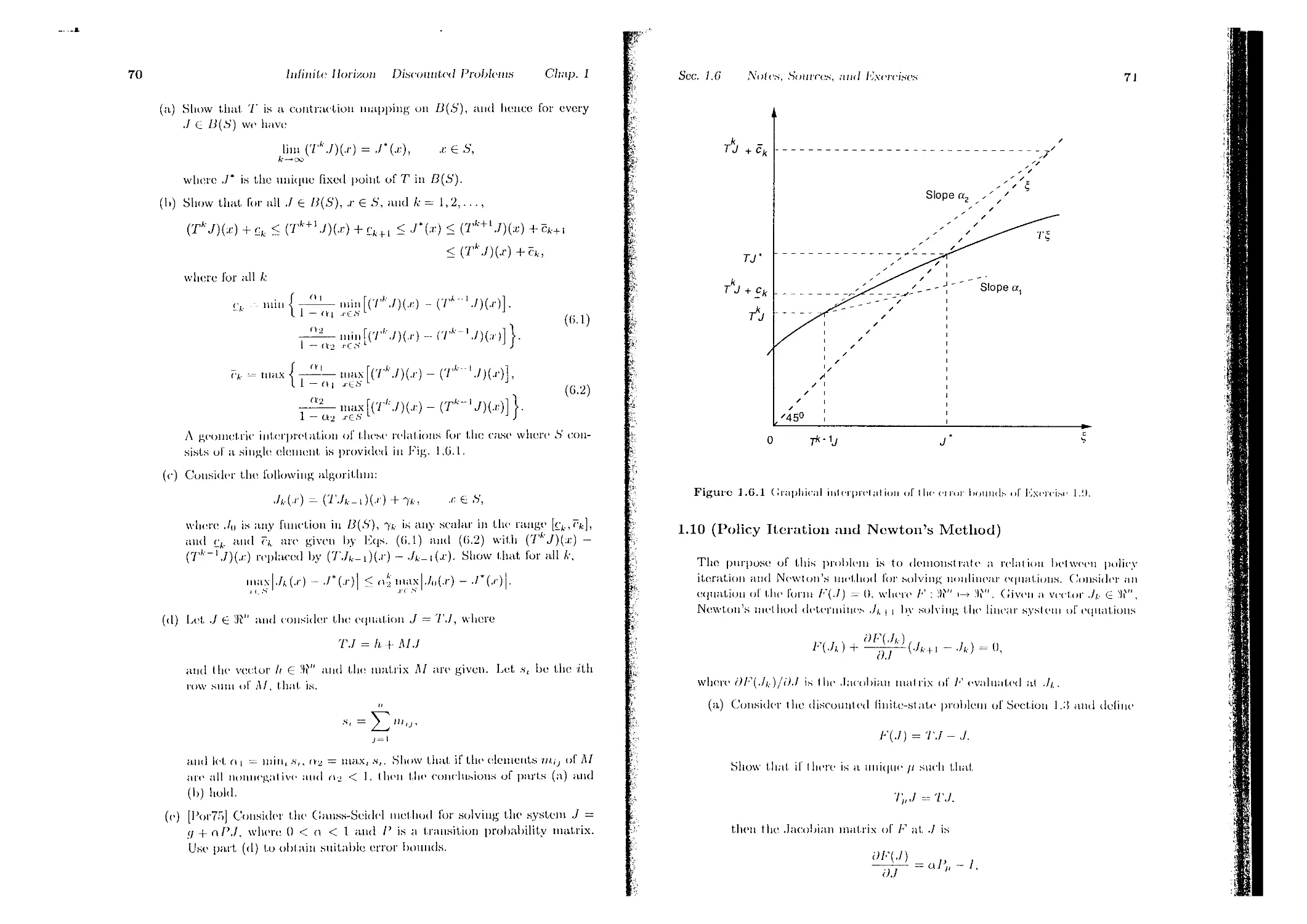
1.6.	Notes. Sources, and Exercises........................p.	61
2.	Stochastic Shortest Path Problems
v 2.1. Main Results...........................................p.	78
2.2.	Computational Methods................................p.	87
2.2.1.	Value Iteration................................p.	88
2.2.2.	Policy Iteration ..............................p.	91
2.3.	Simulation-Based Methods.............................p.	94
2.3.1.	Policy Evaluation by Monte-Carlo Simulation . . . p.	95
2.3.2.	Q-Learning.....................................p.	99
2.3.3.	Approximations.................................p. 101
2.3.4.	Extensions to Discounted Problems..............p. 1-18
2.3.5.	The Role of Parallel Comput ation..............p. 120
2.4.	Notes, Sources, and Exercises........................p. 121
3.	Undiscounted Problems
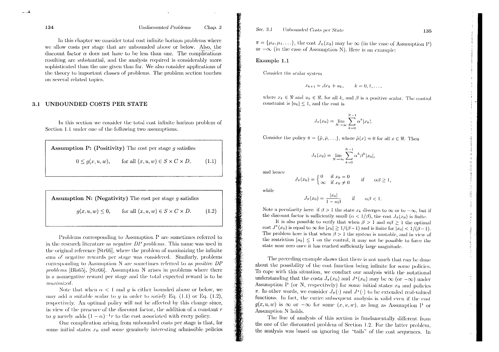
3.1.	Unbounded Costs per Stage?............................p.	134
3.2.	Linear Systems and Quadratic Cost.....................p.	150
3.3.	Inventory Control.....................................p.	153
3.4.	Optimal Stopping......................................p.	155
3.5.	Optimal Gambling Strategies...........................p.	160
». -I
iv	(\>ult4ifs
3.6.	Noustationary and Periodic Problems ...................p.	167
3.7.	Noles, Sources, and Exercises..........................p.	172
4.	Average Cost per Stage Problems
4.1.	Preliminary Analysis...................................p.	181
•1.2. Optimality Conditions.................................p.	lf)l
4.3.	Computational Methods..................................p.	202
4.3.1.	Value Iteration.................................p.	202
4.3.2.	Policy Iteration................................p.	213
4.3.3.	Linear Prograinming..............................p.	221
4.3.4.	Simulation-Based Methods ........................p.	222
4.4.	Infinite State Space ..................................p.	226
4.5.	Notes, Sources, and Exercises..........................p.	229
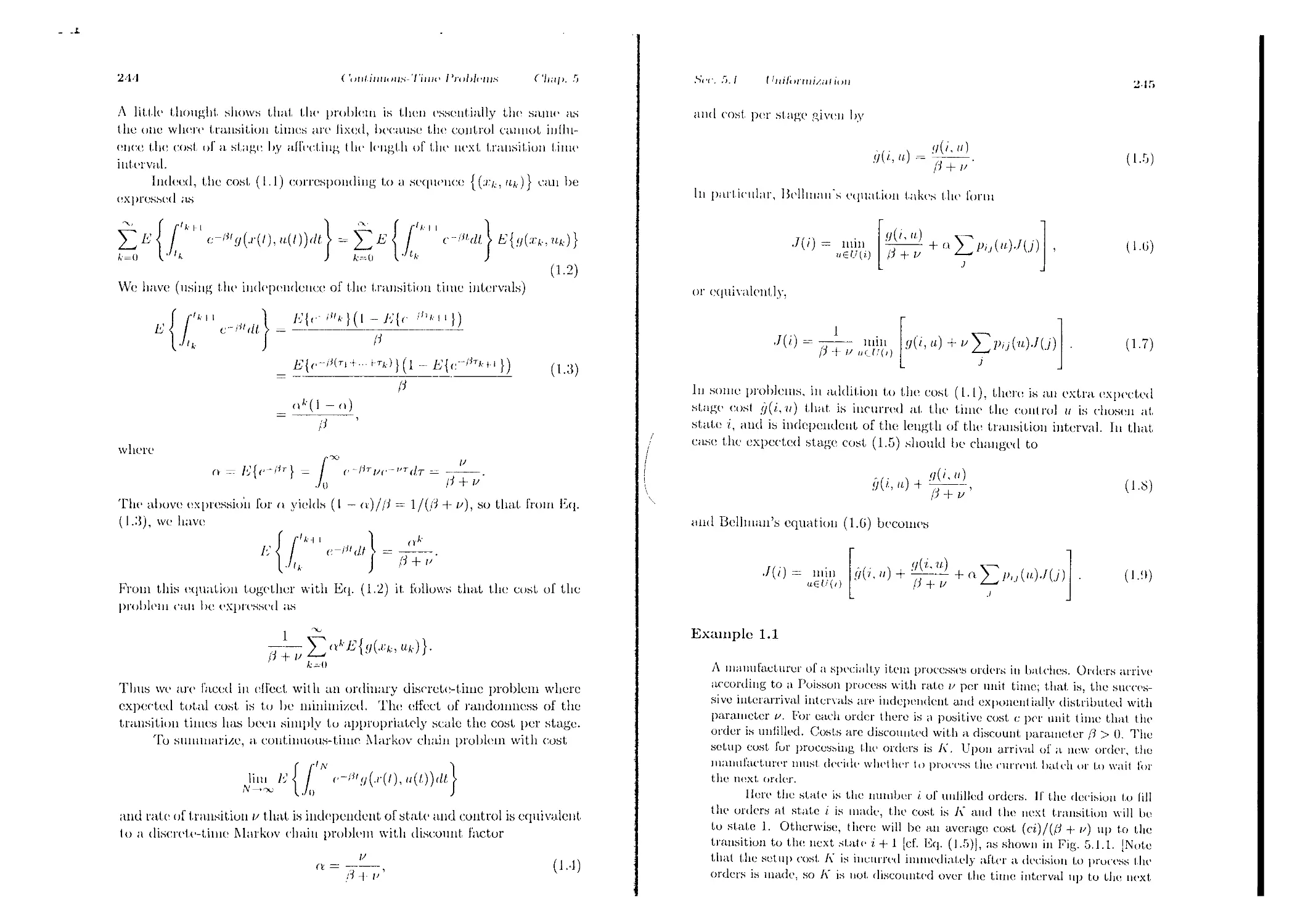
5.	Continuous-Time Problems
5.1.	Uniforniization .......................................p.	212
5.2.	Queueing Applications..................................p.	250
5.3.	Semi-Markov Problems...................................p.	261
5.4.	Notes, Sources, and Exercises..........................p.	273

CONTENTS OF VOLUME 1
1.	The Dynamic Programming Algorithm
1.1.	Introduction
1.2.	The Basic Problem
1.3.	The Dynamic Programming Algorithm
1.4.	State Augmentation
1.5.	Some Mathematical Issues
l.(i. Notes, Sources, and Exercises
2.	Deterministic Systems and the Shortest Path Problem
2.1.	Finite-State Systems and Shortest Paths
2.2.	Some Shortest Path Applications
2.2.1.	Critical Path Analysis
2.2.2.	Hidden Markov Models and the Viterbi Algorithm
2.3.	Shortest Path Algorithms
2.3.1.	Label Correcting Methods
2.3.2.	Auction Algorithms
2.1.	Notes. Sources, and Exercises
3.	Deterministic Continuous-Time Optimal Control
3.1.	Continuous-Time Optimal Control
3.2.	The Hamilton Jacobi Bellman Equation
3.3.	The Pontryagin Minimuni Principle
3.3.1.	An Informal Derivation Using the 11JB Equation
3.3.2.	A Derivation Based on Variational Ideas
3.3.3.	The Minimum Principle for Discrete-Time Problems
3.4.	Extensions of the Minimum Principle
3.1.1.	Fixed Terminal State
3.4.2.	Free Initial State
3.4.3.	Free Terminal Time
.3.4.4	. Time-Varying System and Cost
3.4.5.	Singular Problems
3.5.	Notes, Sources, and Exercises
4.	Problems with Perfect State Information
4.1.	Linear Systems and Quadratic Cost,
4.2.	Inventory Control
1.3.	Dynamic Portfolio Analysis
4.4.	Optimal Stopping Problems
4.5.	Scheduling and the Interchange Argument
1.6.	Notes, Sources, anil Exercises
.1
vi	C'oiitenls
5.	Problems with Imperfect State Information
5.1.	Reduction to the Perfect Information Case
5.2.	Linear Systems mid Quadratic (lost
5.3.	Minimum Variance Cont rol of Linear Systems
5.1.	Sufficient Statistics and Pinite-State Markov Chains
5.5.	Sequential Hypothesis Test ing
5.6.	Notes, Sources, and Exercises
G. Suboptimal anti Adaptive Control
6.1.	Certainty Equivalent and Adaptive Control
6.1.1.	Caution. Probing, and Dual Control
6.1.2.	Two-Phase Control and Identilial>ilitу
(i.	1.3. Certainty Equivalent Control and Identifiability
6.1.1.	Self-liming Regulators
6.2.	Open-Loop Feedback Control
6.3.	Limited Lookahead Policies and Applications
6.3.1.	Flexible Manufacl iiring
6.3.2.	Computer Chess
6.1. Approximations in Dynamic Programming
6.1.1. Discretization of Optimal Control Problems
6.4.2. Cost-to-Co Approximation
6.1.3. Other Approximations
6.5.	Notes, Source's, and Exercises
7. Introduction to Infinite Horizon Problems
7.1.	An Overview
7.2.	Stochastic Shortest Path Problems
7.3.	Discount<'d Problems
7.4.	Average Cost Problems
7.5.	Notes, Sources, and Exercises
Appendix A:	Mathematical Review
Appendix B:	On Optimization Theory
Appendix C:	On Probability Theory
Appendix D:	On Finite-State Markov Chains
Appendix E:	Least-Squares Estimation and Kalman Filtering
Appendix F:	Modeling of Stochastic Linear Systems
ABOUT THE AUTHOR
Dimitri Bertsekas studied Mechanical and Electrical Engineering at
the National Technical University of Athens, Greece, and obtained his
Ph.D. in system science from t he Massachusetts Institute of Technology. He
has held faculty positions with the Engineering-Economic Systems Dept.,
Stanford University and the Electrical Engineering Dept., of the Univer-
sity of Illinois, Urbana, lie is currently Prolessor of Electrical Engineering
and Computer Science at the Massachusetts Institute of Technology, lie
consults regularly with private industry and has held editorial positions in
several journals. He has been elected Fellow of the IEEE.
Professor Bertsekas has done research in a broad variety of subjects
from control theory, optimization theory, parallel and distributed computa-
tion, data communication networks, and systems analysis. He has written
numerous papers in each of these areas. This book is his fourth on dynamic
programming and optimal control.
Other books by the author:
1)	Dynamic Programming and Stochastic Control, Academic Press, !!)“(>.
2)	Stochastic Optimal Control: The Discrete-Time Case, Academic Press.
1978 (with S. E. Shreve: translated in Russian).
3)	Constrained Optimization and Lagrange Multiplier Methods, Academic
Press, 1982 (translated in Russian).
J) Dynamic Programming: Deterministic and. Stochastic Models. Prenti-
ce-Hall, 1987.
.5) Data Networks. Prentice-Hall, 1987 (with R.. G. Gallager; translated
in Russian and Japanese): 2nd Edition 1992.
G) Parallel and Disl ributed Computation: Numerical Methods. Prentice-
Hall, 1989 (with J. N. Tsitsiklis).
7) Linear Network Optimization: .Algorithms and. Codes, M.I.T. Press
1991.

This two-volume book is based on a. first.-year gradual,e course' on
dynamic programming and optimal control that 1 have taught, lor over
twenty years al. Stanford University, t he University of Illinois, and the Mas-
sachusetts Institute of Technology. The course has been typically attended
by students from engineering, operations research, economics, and applied
mathematics. Accordingly, a principal objective of the book has been to
provide a. unified treatment of the subject., suitable for a broad audience.
In particular, problems with a continuous character, such as stochastic con-
trol problems, popular in modern control theory, arc simultaneously treated
with problems with a discrete character, such as Markovian decision prob-
lems, popular in operations research. Furthermore, many applications and
examples, drawn from a broad variety of fields, are discussed.
The book niay be viewed as a greatly expanded and pedagogically
improved version of my 1987 book “Dynamic Programming: Deterministic
and Stochastic Models," published by Prcntice-Ibill. I have included much
new material on deterministic and stochastic shortest, path problems, as
well as a new chapter on continuous-time optimal cont rol problems and the
Pontryagin Maximum Principle, developed from a dynamic programming
viewpoint. 1 have also added a fairly extensive exposition of simulation-
based approximation techniques for dynamic programming. These tech-
niques, which are often referred to as “neuro-dynamic programming" or
"reinforcement learning,” represent a breakthrough in the practical ap-
plication of dynamic programming to complex problems that, involve I hi'
dual curse of large dimension and lack of an accurate mathematical model.
Other material was also augmented, subst.antia.lly modified, and updated.
With the new material, however, the book grew so much in size I hat it.
became necessary to divide it into two volumes: one on finite horizon, and
the other on infinite horizon problems. This division was not, only nat ural in
terms of size, but. also in terms of style and orient at ion. The first, volume is
more oriented towards modeling, and the second is more oriented towards
mathematical analysis and computation. To make the first volume self-
contained for instructors who wish to cover a. modest amount, of infinite
horizon material in a course that is primarily oriented towards modeling,
-. .1
x	Preface
conceptualization, and finite horizon problems, I have added a final chapter
that provides an introductory treatment of infinite horizon problems.
Many topics in the book are relatively independent of the others. 1‘or
example Chapter 2 of Vol. 1 on shortest path problems can be skipped
without loss of continuity, and the same is true for Chapter 3 of Vol. 1,
which deals with continuous-time optimal control. As a result, the book
can be used to teach several different types of courses.
(a)	A two-semester course that covers both volumes.
(b)	A one-semester course primarily focused on finite horizon problems
that covers most of the first volume.
(c)	A one-semester course focused on stochastic optimal control that, cov-
ers Chapters 1, 4, 5, and 6 of Vol. 1, and Chapters 1, 2, and 4 of Vol.
11.
(c)	A one-semester course that covers Chapter 1, about 50% of Chapters
2 through (i of Vol. I, and about 70% of Chapters 1, 2, and 4 of Vol.
If. This is tiie course I usually teach at MIT.
(d)	A one-quarter engineering course that covers the first, three chapters
and parts of Chapters 4 through 6 of Vol. I.
(e)	A one-quarter mathematically oriented course focused on infinite hori-
zon problems that covers Vol. II.
7dic mathematical prerequisite for the text, is knowledge of advanced
calculus, introductory probability theory, and matrix-vector algebra. A
summary of this material is provided in the appendixes. Naturally, prior
exposure to dynamic system theory, control, optimization, or operations
research will be helpful to the reader, but, based on my experience, the
material given here is reasonably self-contained.
The book contains a large number of exercises, and the serious reader
will benefit greatly by going through them. Solutions to all exercises are
compiled in a manual that is available to hist rectors from Athena Scientific
or from the author. Many thanks are due to the several people who spent
long hours contributing to this manual, particularly Steven Shreve, Eric
Loiedennan, Lakis Polymenakos, and Cynara \Vu.
Dynamic programming is a conceptually simple technique, that can
be adequately explained using elementary analysis. Yet a mathematically
rigorous treatment, of general dynamic programming requires the compli-
cated machinery of measure-theoretic probability. My choice has been to
bypass the complicated mathematics by developing the subject in general-
ity, while claiming rigor only when the underlying probability spaces are
countable. A mathematically rigorous treatment, of the subject is carried
out ill my monograph "Stochastic Optimal Control: The Discrete Time
Case,'’ Academic Press, 1978, coauthored by Steven Shreve. This mono-
graph complements the present text and provides a solid foundation for the
Preface	xi
subjects developed somewhat informally here.
Finally, I am thankful to a number of individuals and institutions
for their contributions to the book. My understanding of the subject was
sharpened while ! worked with Steven Shreve on onr I97S monograph.
My interaction and collaboration with John Tsitsiklis on stochastic short-
est. paths and approximate dynamic programming have been most valu-
able. Michael Caramanis, Emmanuel I'eruandcz-Gaucherand, Pierre Hum-
bid, Lennart Ljimg, and John Tsitsiklis taught from versions of the book,
and contributed several substantive comments and homework problems. A
number of colleagues offered valuable1 insights and information, particularly
David Castanon, Eugene Feinberg, and Krishna Pattipati. NSF provided
research support. Prentice-Hall graciously allowed the use of material from
my 1987 book. Teaching and interacting with the students at. MIT haw1
ke.pt up my interest and excitement for the subject.
Dimitri I’. Bertsekas
bertsekas (.о1) ids. mit.edu

1
Infinite Horizon -
Discounted Problems
Contents
1.1.	Minimization of Total Cost - Introduction.............p.	2
1.2.	Discounted Problems with Bounded Cost per Stage ... p. 9
1.3.	Finite-State Systems - Computational Methods..........p.	16
1.3.1.	Value Iteration and Error Bounds................p.	19
1.3.2.	Policy Iteration................................p.	35
1.3.3.	Adaptive Aggregation............................p.	44
1.3.4.	Linear Programming..............................p.	49
1.4.	The Role of Contraction Mappings......................p.	52
1.5.	Scheduling and Multiarmed Bandit Problems.............p.	54
1.6.	Notes, Sources, and Exercises.........................p.	64

2	liilinil.e Horizon Discounted Problems C7iap. I
This volume focuses on stochastic optimal control problems with an
infinite number of decision stages (an infinite horizon). An introduction
to these problems was presented in Chapter 7 of Vol. 1. Here, we provide:
a more comprehensive analysis. In particular, we do not assume a finite
number of states and we also discuss the associated analytical and compu-
tational issues in much greater depth.
We recall from Chapter 7 of Vol. I that then' are four classes of infinite
horizon problems of major interest.
(a) Discounted problems with bounded cost per sl.age.
(1>) Stochastic shortest pat h problems.
(c) Discounted and undiseounted problems wit h unbounded cost, per st age.
(d) Average cost per stage problems.
Each one of the first four chapters of the present, volume considers one
of tile above problem classes, while tin' final chapter extends t he analysis to
continuous-time problems with a countable number of states. Throughout
this volume we concentrate on the perfect, information case, where each
decision is made with exact knowledge' of the current system state. Im-
perfect state informat ion problems can be treated, as in Chapter 5 of Vol.
1. I>y reformulation into perfect, informal ion problems involving a sufficient,
statistic.
1.1 MINIMIZATION OF TOTAL COST - INTRODUCTION
We now formulate the total cost minimization problem, which is the
subject, of this chapter and t.ho next two. This is ini infinite horizon, sta-
tionary version of the basic problem of Chapter 1 of Vol. I.
Total Cost Infinite Horizon Problem
Consider the stationary discrete-time dynamic system
•'g-n =/(ag, u/,-, tag.), k = 0,1,...,	(1.1)
where for all the state .ig is an clement of a space S', the control оis
an element of a space C, and the random disturbance ng is an ('lenient,
of a space D. We assume that D is a countable set. The control ng. is
constrained to take values in a given nonempty subset U(:r.k) of C, which
depends on the current slate .г/,, [a/,, о ('(.ig), lor all ,/g. C 5]. The random
disturbances ug..к = 0, I,..., have identical statistics and are characterized
by probabilities P(- | .ig, ig) defined on D, where | Xk- iik) is the
Sac. 1.1
Minimization ol Total Cost Introduction
3
probability ol occurrence of Wk, when the current, stair: and cont rol are .17.
and u.f,.. respectively. The probability of «,7. may depend explicitly on .17.
and Hi,, but. not, on values of prior disturbances 117. ।......u\}.
Given an initial state xo, we want to find a policy тг = {/ro,//1,..
where /17 : S t-» C, fik^Xk) G U(xk)> for all € S, к -= 0,1................ that,
minimizes t he cost, function f
(N-l	4
Л(-Со) = lim E < V <>ау(.га-.//а(-'ч), 117.) > .	(1.2)
N—>c*j "’a-	I	I
fc=0,L,,..	I fc=0	)
subject to the system equation constraint (1.1). The cost per stage у :
S x C x D 1—> 'li is given, and cr is a positive scalar referred to as t.he
discount factor.
We denote by И the set of all admissible policies тг, that is, the set of
all sequences of functions тг = {po,/<r,   } with //7 : S C, IIk-(x) e U(x)
for all x E S, к ~ (), 1.... The opt imal cost, funct ion ./* is delined by
J*(.r) = min,/тг(х), .r E S.
wen
A stationary policy is an admissible policy of the form тг —
and its corresponding cost function is denoted by ,/p. For brevity, we
refer to {ц.р. ..} as the stationary policy /1. Wc say that /1 is optimal if
Jii(x) = .7*(.i.') for all states x.
Note that, while we allow arbitrary state and control spaces, we re-
quire that the disturbance space be countable. This is necessary to avoid
the mathematical complications discussed in Section 1.5 of Vol. 1. The
countability assumption, however, is satisfied in many problems of inter-
est, notably for deterministic optimal control problems anil problems with
a finite or a countable number of states. For other problems, our main
results can typically be proved (under additional technical conditions) by
following the same line of argument as the one given here, but also by
dealing with the mathematical complications of various measme-theoret ic
frameworks; see [BeS78].
The cost Л(.г0) given by Eq. (1.2) represents the limit, of expected
finite horizon costs. These costs are well defined as discussed in Section
f In what follows we will generally impose appropriate assumptions on the
cost per stage <1 and the discount factor n that, guarantee that the limit delining
the total cost ./„(.t’o) exists. If this limit is not known to exist, we use instead
the dclinit ion
Г N -1
E(xi>) = lim sup E <2 O1 </(.17,,/ц;(.17.), 117.)
у ..^	"4	i—1
i.	11.1,	</ u
.. .ж
4	Horizon Discounted Problems Chap. I
1.5 of Vol. 1. AuotlicT possibility would be to minimize over 7r the expected
infinite horizon cost
F S	П’а) > .
* -<>.*!,. . I* 0	J
Such a cost, would require а Гаг more complex mathematical formulation (a
probability measure' on the space of all disturbance sequences; see [BeS"8]).
However, we mention that, under the assumptions that, we will be using,
the preceding expression is equal to the cost given by Eq. (1.2). This
may be proved by using the monotone convergence! theorcin (see Section
3.1) and other stochastic convergence theorems, which allow interchange of
limit and expectation under appropriate! conditions.
The DP Algorithm for the Finite-Horizon Version of the Problem
Consider any admissible polit y rr = {//.o,/<i,...}, any positive integer
JV. and any function ./ : S l)i. Suppose that we accumulate the costs of
the lirst. N stages, and to them we add the terminal cost oa'.7(.cn), for a.
total expected cost
(	N' 1	1
Г s o-v./(.r,v) + У7 <|/'.'/('''А’,/'а (.'т). if*) г •
* o/l.... I	*-ll	J
The minimum of this cost over тг can be calculated by starting with <yN J(x)
and by carrying out N iterations of the corresponding DP algorithm ol
Section 1.3 of Vol. I. This algorithm expresses t.he optimal (Ar — /c)-stage cost
starting from state .r, denoted by ./* (.r), as the minimum of the expected
sum of the cost, of stage V — k and t.he optimal (V — A: — ])-st.age cost
starting from the next stale. It. is given by
.//,.(./)— min	U, 1 w, «’)) }•	= 0, 1, • • • , N-1.
ned(.i)
(1.3)
with the. initial condition
Av (') = ол'./(.г).
For all initial stales .r, the optimal /V-st.age cost, is the function ./i>(.c)
obtained from t.he last, step of the DP algorithm.
Let. us consider for all A' and .r, the functions given by
.	-Lv-*(.f)
Sec. 1.1
Miuimizat ion of Total Cost Inf roeliicf.ioi)
□'lien is the optinitil A'-stage cost, Jo(.r), while the DI’ recursion (I ..3)
can lie equivalent ly be written in terms of the functions If. as
VA.+ i(.r) = min /r{e/(.r, a, ui) + oVf. (J'(;r. a, <(')) }, /.’= 0. 1, . . . , .V - 1.
aCt'(.r)
with the initial condition
lh(.r) = ./(.r).
The above algorithm can be used to calculate? all. the optimal finite
horizon cost functions with a single. DI’ recursion. In particular, suppose
that we have computed the optimal (Ar — l)-st,age cost function V\_|.
Then, to calculate the optimal Л'-stage cost function Vn, we do not need
to execute1 the A’-stage DP algorithm. Instead, we can calculate1 V\ using
the one-stage iteration
!>(.;)= min u. «’) +ol'.v-i «.«'))}.
More generally, starting with some1 terminal cost function, we1 can
consider applying repeatedly the1 DP iteration as above. With each appli-
cation, we will be? obtaining the? optimal cost function of some? finite: horizon
problem. The1 horizon of this problem! will be1 longer by one1 stage1 eiver the1
heaizon of the prcceeling problem. Note- that, this e-enivenience1 is possible1
only because we are dealing with a stationary system anel a common cost
function g for all stage?s.
Some? Shorthand Notation
The: precexling mctlmel of calculating finite horizon optimal exists mo-
tivates the introeluction of twei mappings that play an impeirtant theoretical
role anil proviele1 a convenient shorthand notation in expressions t hat woulel
be toe> complicated to write? eitherwise.
For any function : S’ e—> 3?. we1 consider the1 function obtaine'il by
applying t.he Di’ mapping to ./, anel we- de'imte1 it by f
= min E u, ic) + aj(f(.r, a, u-)') } , j: € S'.	(1-1)
u'
Since1 (T,/)(•) is itself a, funct ion elefiiietel on the state space’ S', we1 view T as
a mapping that transforms the function ./ on .S' into t he lunction 7’./ on .S'.
Neite1 that T.J in the optimal cost function for the on.c-sla.gc probit in that
has stage cost, g and terminal cost. n.7.
j Whenever we1 use the mapping T, we1 will impose’ sufficient assumpliems Ie>
guarantee? that the cxpectexl value involveel in Eq. (1.1) is well elefineel.
6
bilinite Horizon Discounted Problems
(Imp. I
Similarly, for any funct ion .] : ,S' >—> iff and any control function p. :
5 C, we denote
(7;,./)(.z:) = /;{z/(.r,/z(.r), zzz) п-.7(/(.г,	<<’)) } , G S.
IV
Again, T;1.7 may be viewed as the cost function associated witli /z for the
one-stage problem that has stage cost g and terminal cost о J.
We will denote by Tk the composition of the mapping T with itself к
times; that is, for all к we write
(7'*,/)(.r)= (7’(7'A->./))(.;;), x G 5.
Thus Tk,) is the function obtained I>y applying tdie mapping 7’ to the
function Tk~1./. For convenience, we also write
(T"J)(x)	,7(x), .rcS.
Similarly, I’j'i.i is defined by
(7’Д./)(.г)= (7;,(7;;-l.7))(.r), xGS,
and
(Tz?.7)(,:) = .7(.r), X G S.
It can be verified by induction that (7,/,',7)(x) zs the optimal cost for the.
к-stage, о-discounted problem until initial state, x, cost per stage g, and
terminal cost Junction a1'./. Similarly, (TfJ)).!:) is the cost of a. policy
for the same problem. To illustrate the case where к = 2, note
that
(7’2.7)(x) = min E{u(x, a, in) 4- о (T .J) (ffr, a, zz;))}
llt£(/(x) 11!
= min ZJ < z/(.z:, Un, zz'o) + a min 75 •{ g(f(x, zzn, w(l), щ, Wi)
1/oGZdr) 1'4, I	“0."’<())'Z’l I
+ O-7(/(/(.r, an, ZZ’o), ZZ.,, zz-,)) 11
= mill Id < <i(.r. Ho, Ii’u) + min E\<ig(f (>'., Un,up), щ ,Wi)
H'u I	i'I tG(7(r,<i|).l,,o)) "’I t
+ <'2./	"0, »',)). zz,, zz-,)) | j.
The last expression can be recognized as the DP algorithm for the 2-stage,
o-discounted problem with initial state x, cost per stage g, and terminal
cost function zi2.7.
Finally, consider a X'-stage policy те = {/'<». Mi,    , pi,-i}. Then, the
expression	   7’/IA, ^.))[х) is delined recursively lor z = 0,... I: — 2
by
СЛо he н ''' ho. -1 )(•'') ~ СЛо (he 11 ' ‘iic i-^))(a;)
and represents the cost of the policy тг for the к-stage, a-discounted problem
with initial state x, cost, per stage g, auel terminal cost, function akJ.
Sec. 1.1
Miniuiiziition ofTolnl Cost hit i oiIik I ion
7
Some Basic Properties
The following monotonicity property plays a fundamental role in the
developments of tins volume.
Lemma 1.1: (Monotonicity Lemma) For any functions J : .5' >—>
Ji and J' : S JR, such that
,7(.r) < ./'С7-'), for all ;i: г S’,
and for any function ц-.S^C with p(x) e P(-r), for all a: G S, we
have
(Tfc J)(.r) < (7X/')(.r), for all .r £ S, k = 1, 2,...,
(7p)(.r) < (T/f J')(.r), for all G 5, k =1,2,...
Proof: The result follows by viewing (TkJ)(.n) and (7’(('.7)(.r) as A ’-stage
problem costs, since as the terminal cost, function increases uniformly so will
the A'-stage costs. (One can also prove t he lemma by using a straight forward
induction argument.) Q.E.D.
For any two functions J : S >—» ft and .J' : 5	3i, we write
J < .1’	if J(.c) < ./'(.r) for all •<’ G S’.
With this notation, Lemma 1.1 is stated as
.!<.]'	=> TkJ < Tk.I', /,’=1,2.................
.]<]'	=>	T(c./<Tp./',	/.’=1,2,...
Let us also denote by c : S'R the unit function that takes the value
1 identically on S’:
e(.r) = 1, for all ,r € S.	(1.6)
We have from the definitions (1.4) and (1.5) of T and 7’;,, for any funct ion
J : S >—> 4? and scalar r
(T(./ + re))(.r) = (T./)(.r)4-or, .rG.S,
+ /’<’))(./.•) = (/),./)(.r) + о;;	.1- G s.
More generally, the following lemma can be verified by induction using the
preceding two relations.
-. -Ж
Iiilinite Horizon Discounted Problems C'liap. 1
Lemma 1.2: For every A:, function J : S' н and scalar r, we have	))i, stationary policy //.,	
(Tfc(J + rc))(.c) = (TkJ)(x) + akr,	for all x e S',	(1.7)
(7;A(J + r())(.r) = (7;'.J)(,:)+nAr,	for all x 6 S’.	(1.8)
A Preview of Infinite Horizon Results
It is worth at this point to speculate on the type of results that we
will he aiming for.
(а)	Convcrqtmce of the DP Alt/oritlmi. Let Jo denote the zero function
[Jo (•'•') - 0 for all Since the infinite horizon cost, of a policy is, by
definition, the limit, of its /.'-stage costs as /.' —> oe, it is reasonable to
speculate that the optimal infinite horizon cost is equal to I,he limit
of the optimal L-stage costs; that, is,
J*(.r) =	x e 5.	(IT)
This means that if we start, with the zero function Jo and iterate with
the DP algorithm indefinitely, we will get. in the limit tin; optimal cost,
function J*. Also, for о < 1 and a bounded function J, a terminal
cost, ak J diminishes with /.:, so it. is reasonable to speculate that, if
<1 < 1,
J‘(.r) — lim (7'A'J)(.r), for all ,r S' and bounded functions J.
(1.10)
(b)	Hcll.ni.au s Equation. Since by definition we have for all x 6 S
(7'A и Jn)(.r) = min A {//(.c. a, w) + o(TA Jo)(/(x, u, w)) } , (l.H)
i/CO’(.г) u-
it. is reasonable to speculate that if 1mm _ ю Tk Ju = J* as in (a) above,
then we must have by taking limit, as k —> oo,
./*(.;:)— min	a, iv) + a J* (f(x, n, w))}, x. e S’, (1.12)
lit (-'(.r) in
or, equivalently,
J*=7’J*.	(1.13)
This is known as Bellman's equation and asserts that the optimal
cost function J* is a fixed point of the mapping T. We will see that
tier. 1.2
Disciitmled I’го/di'iiis with Hounded (-05/ per .Stage
!)
Bellman’s equation holds for all the total cost minimization problems
that we will consider, although depending on our assumptions, its
proof 1-пи be quite complex.
(c)	('liararh Ti.zahon tij OiiUmal Slalioiuin) I 'olicics. If we view Bellman’s
equation as the DP algorithm taken to its limit as k tx. it is
reasonable' to speculate that it attains t he minimum in the right -
hand side of Bellman’s equation for all .r, t hen the stationary policy
// is optimal.
Most of the analysis of total cost infinite horizon problems revolves
around the above three issues and also around the issue' of ellicient com-
putation of .7* and an optimal stationary policy. Bor the discounted cost
problems with bounded cost per stage considered in this chapter, and for
stochastic shortest path problems under our assumptions of Chapter 2. the
preceding conjectures are correct. For problems with unbounded costs per
stage and for stochastic shortest path problems where our assumptions of
Chapter 2 are violated, there may be counterintuitive mathematical phe-
nomena that invalidate some of the preceding conjectures. This illustrates
that infinite horizon problems should be approached carefully and with
mathematical precision.
1.2 DISCOUNTED PROBLEMS WITH BOUNDED COST PER
STAGE
We now discuss the simplest, type of infinite horizon problem. We
assume the following:
Assumption D (Discounted Cost - Bounded Cost per Stage):
The cost per stage <j satisfies
|</(x, w, w)| < Л/, for all (r, u, w) e S x C x D, (2.1)
where M is some scalar. Furthermore, 0 < a < 1.
Boundedness of I.he cost, per st age is not as restrict! ve as might appear.
It holds for problems where the spaces S, C, anil D are finite sets. Even
if these spaces are not finite, during the computational solution of the
problem they will ordinarily be approximated by finite sets. Also, it is
often possible to reformulate the problem so that it. is defined over bounded
regions of the state and control spaces over which the cost is bounded.

10	/н/нп/с lhni/,i>u I )isci unit < ‘t I I ’i < tblemx	I
The following proposition shows that the DP algorithm converges to
the optimal cost, function ./* for an arbitrary bounded starting function
This will follow as a, consequence of Assumption D, which implies that the
"tail'' of the cost after st,age N, that is,
Г л
E < ^2	«г)
4-400	U;=/V
diminishes to zero as N —> oo. Furthermore, when a terminal cost, <\N
is added to the Л'-stage cost, its effect diminishes to zero as N oo if J
is bounded.
Proposition 2.1: (Convergence of the DP Algorithm) For any
bounded function ./ : S *—> !)i, the optimal cost function satisfies п -t ,
J‘(./:)= lim (TNJ)(:r), for all j: e S. (2.2)
Proof: For every positive integer Z\, initial state .r(> C .S', and policy тг —
{/to, /zi,. . .}. we break down the cost E(.i'a') into the portions incurred over
the first. l\ stages and over t he remaining st,ages
С V - 1	'j
Л(.со) = lim E< 52па,.9(л-,/Ц-(а),1^) ?
l а —о	)
f к' -1	>
- E < пМ-'Чи/М-а) jo.) >
I A'--(l	J
p'-l	A
4- Jini E <	u’a) > •
~4°° Ia=A’	J
Since by Assumption D we have |</(.rt,//а (.га ), ttg ) | < Л/, we also obtain
p -1	V	rv
lim E < Y oA'.<7(j\.,//,t.(.rA:), utfc) > < M Y ak = -----------.
l А — /V	)	k=K
Using these relations, it follows that
M-nO - ------------ол ni;tx||
I - u	.ct 5 ‘
Г	Д 1	1
<	E < (\к.](.гк) + У j	u’k) >
V	A:^()	J
a/cA/
<	.Лг(.'о) Ь ------1- inaxl J(.v;)|.
1 — о	.rt s ‘	1
Sec. 1.2
I )i,s< < unit < ’< I /’/<»/>/(/jj.-. with lit и 11 и /<•< I ( *<».«./ /»<•/ S/.U4-
I I
By taking the minimum over 7Г, we obtain for all .z.’o and A',

<>M7
1 — a
— aK max|.7(z)|
nKif
<	4- ------к (\K' max|./(.r)
and by taking the limit as A' —> oc, the result- follows. Q.E.D.
Note that based on the preceding proposition, t he DP algorithm may
be used to compute at least an approximation to ,7*. This computational
method together with some additional methods will be examined in the
next section.
Given any stationary policy /i, we can consider a uiodilied discounted
problem, which is the same as t.he original (except, that, the control constraint
set contains only one element, for each state the control //.(j:); that is,
the control constraint set is U(x) = {//.(r)} instead of U(x). Proposition
2.1 applies t.o this modified problem and yields the following corollary:
Corollary 2.1.1: For every stationary policy p, the associated cost
function satisfies
= Jim (T;f J)(.r), for all x e S.	(2.4)
The next proposition shows that .7* is the unique solution of Bellman's
equation.
Proposition 2.2: (Bellman’s Equation) The optimal cost func-
tion J* satisfies
J*(.r) = min E{g(x, u, w) + aJ* (j(x, u, «')) }, for all x e S.
(2.5)
or, equivalently,
J*=TJ*.	(2.6)
Furthermore, J* is the unique solution of this equation within the class
of bounded functions.
-..Л
12	infinite Horizon — Discounted Problems Chap. 1
Proof: from Eq. (2.3), we have lor all .r E S and N,
where ./ц is the zero function [./o(:r) = 0 for all .r £ S]. Applying the
mapping 7’ to this relation and using t.he Monotonicity Lemma 1.1 as well
as Lemina 1.2, we obtain for all .r E 5 and N
oN + 'l\l	+
(7’./*)(.r) - Ц---- < (T"+LJ())(.r) < (7’.7’)(.,;) + ----.
1—0	1—0
Since (TN • 1 .7o)(.r) converges to ./*(.r) (cf. Prop. 2.1), by taking the limit
as N —> oo in the preceding relation, we obtain J* = TJ*.
To show uniqueness, observe that if J is bounded and satisfies J =
7’.7, then .7 = lini.v .TN,/, so by Prop. 2.1, we have ,7 = J*. Q.E.D.
Based on t.he same reasoning we used t.o obtain Cor. 2.1.1 from Prop.
2.1, we have:
Corollary 2.2.1: For every stationary policy p, t.he associated cost
function satisfies
J,,,(x) = E{<7(:i;,/z(;r), w) + oJ;i(/(.r,/((.r), w))}, for all z e S,
w k
(2-7)
or, equivalently,
I — т I
Furthermore, ,7M is the unique solution of this equation within the class
of bounded functions.
The next, proposition characterizes stationary optimal policies.
Proposition 2.3: (Necessary and Sufficient Condition for Op-
timality) A stationary policy p is optimal if and only if //. (.r) attains
the minimum in Bellman’s equation (2.5) for each e S\ that is,
7’.7* --7),./*.	(2.S)
Proof: If 7’.7* = 7),./*, then using Bellman’s equation (.7* = TJ*), we
have .7* = T/iJ*, so by the uniqueness part of Cor. 2.2.1, we obtain .7* — J,r,
Sec. 1.2 Discounted Problems with Bounded Cost per Stage	13
that, is, p is optimal. Conversely, if the stationary policy p is optimal, we
have, J* = ,/ц. which by Cor. 2.2.1, yields ./* = 7),./*. Combining this with
Bellman's equation (,/* = TJ*), we obtain TJ' — I),J*. Q.E.D.
Note that Prop. 2.3 implies the existence of an optimal stationary
policy when the minimum in the right-hand side of Bellman's equation is
attained for all .r 6 .9. In particular, when U(.r) is finite for each ,r C .S', an
optimal stationary policy is guaranteed to exist.
We finally show the following convergence rate4 est imate’ for any bounded
function J:
inax|(7't'./)(.r) — J*(,r)| < (J- max| J(.r) - ./’'(;/•)]. k = 0, I, . . .
This relation is obtained by combining Bellman’s equation and the following
result:
Proposition 2.4: For any two bounded functions J : S J' :
S e-» 3?, and for all к = 0,1,..., there holds
max|(7’A: J)(.r) — (T’M')(a,)| < оЛ тах|,7(ж) — ,7'(a;)|.	(2.9)
Proof: Denote
r = “дФС'') - •/,(-'-)|-
Then we have
J(.r) - c < J'(.r) < J(j:) + c, ;r £ S.
Applying T1- in this relation and using the Monotonicity Lemina 1.1 as well
as Lemma 1.2, we obtain
рт.ф) - o'T < (Tfc./')(.r) < (TC/)(.t-) + <J-c, ,r & S.
It follows that
|(7*./)(.r)-(7’C7')(.r)| <cJc, .ceS.
which proves t.he result. Q.E.D.
As earlier, we have:
Infinite Horizon Discounted Problems Cluip. I
...л
Corollary 2.4.1: For any two bounded functions J : S >—» K, J' :
S >—» li, and any stationary policy /1, we have
шах|(Тд J)(x) -	< ak max| J(x) - J'(x)|, к = 0,1,...
т. £ .S’	tr G S
Example 2.1 (Machine Replacement)
Consider an infinite horizon discounted version of a problem we formulated
in Section 1.1 of Vol. 1. Here, we want to operate elliciontly a machine that
can be in any one of n stat.es, denoted 1,2,	State 1 corresponds to a
machine in perfect condit ion. The transition probabilities ptJ are given. There
is a cost y(/’) for operating for one time period the machine when it. is in state
L The options at the start of each period are to (a) let the machine operate
one more period in the state it currently is, or (b) replace the machine with a
new machine (state 1) at a cost R. Once replaced, the machine is guaranteed
to stay in state 1 for one period; in subsequent periods, it may deteriorate
to state's j > 1 according to tin* transit ion probabilities pij. We assume an
infinite horizon and a discount factor о £ ((), 1), so the theory ol this section
applies.
Bellman’s equation (cf. Prop. 2.2) takes the form
(i) = min
/? + .</(!)+ <».7*(1), <;(:)+ <i
By Prop. 2.3, a stationary policy is optimal if it replaces at. states i where
/?	o-C(l) <	-I- O ) J'u-C(j),
and it does not replace at states i where'
H l-.y(l) t o./*(l) <j(i) + O Vpo-F(j).
We can use' the convergence of t he DP algorithm (cf. Prop. 2.1) to
characterize the optimal cost function using properties of the finite horizon
cost functions. In particular, the DP algorithm starting from tin» zero function
takes the* form
/(.(/) - 0,
(7’./„)(t) = min |Л + y(l). </(/)],
Ser. /..3 Finite-Stele Systems C\>ni/>iil;>Li<ni;il Methedx
(Ta./0)(z) = min I\ 4- .7(1) + (\(Tk -l./o)(l), 1/(0 -1-o ^	'
./^1
Assume that g(i) is nondecreasing in /, and that the transition probabilities
satisfy
n	n
- 1, • ,- 1.
for all functions ,/(i), which arc monotonically iiondccrcasing in i. It can be
shown that this assumpt ion is satisfied if and onl.y if, for every A:. У'( ki>,,
is monotonically nondecreasing in i (see [Hos83b|, p. 252). The assumption
(2.10) is satisfied in particular if
P,j = 0, if j < i.
i.e., the machine cannot go to a bel ter slate wit h usage, and
1>,j <	if i < J,
i.e., there is greater chance of ending at a bad state j if we start at a worse
state i. Since //(/) is noildecreasing in i. we have t hat ('/’,/<,)(/) is nondecreasing
in i, and in view of the assumption (2.10) on the transition probabilities, the
same is true for (7’2./,,)(i). Similarly, it. is seen that, for all Ar, (Tk.)„)(/) is
iiondccrcasing in i and so is its limit
,/‘(i) = (Нп^(7’‘-./„)(,).
This is intuitively clear: the.' optimal cost should not decrease as the machine
starts at a worse initial state. It follows that the function
.</(/) -I- О ,./•(./)
is nondecreasing in i. Consider the set. of slates
I « + .<;(!) 4-o,7’(l) < </(<) +	/*(./') j ,
and let.
.» __ f smallest state in S'h if Sit is nonempty,
I 11 + 1	otherwise.
Then, an optimal policy takes the form
replace if and only if 1 > «*,
as shown in 1’ig. 1.2.1.
16
InlhiiU' lloij/лч! Discounted Problems	I
..I
Replace
Figure 1.2.1 Determining the optimal policy in the machine replacement exam-
ple.
1.3 FINITE-STATE SYSTEMS - COMPUTATIONAL METHODS
In this section we discuss several alternative approaches for numeri-
cally solving t he discounted problem with bounded cost per stage. The first
approach, value iteration, is essentially the DP algorithm and yields in the
limit the optimal cost function and an optimal policy, as discussed in the
preceding section. We will describe some variations aimed at accelerating
convergence. Two other approaches, policy iteration and linear program-
ming, terminate in a. finite number of iterations (assuming the number of
states -md controls are finite). However, when the number of states is large,
these approaches are impractical because of large overhead per iteration.
Another approach, adaptive aggregation, bridges the gap between value
iteration and policy iteration, and in a sense combines the best features of
both methods.
In Section 2.3 we will consider some additional methods, which are
well-suited for dynamic systems that, are lim'd to model but, relatively easy
to simulate. In particular, we will assume in Section 2.3 that the transition
probabilities of t.he problem are unknown, but, the system’s dynamics and
cost structure can be observed through simulation. We will then discuss
the methods of temporal diflcrences and Q-lcaniing, which also provide
conceptual vehicles for approximate forms of value iteration and policy
Sec. I.:’,
1чilil.i'-St:it <• Sv.sf enis	( \>ni/>nl:il ioinil Met In и/s
17
iteration using, for example, neural networks.
Throughout this section we assume a discounted problem (Assump-
tion D holds). We further assume that t lit' stale, control, and disturbance
spaces underlying the problem are finite sets, so that we are dealing in
effect with the control of a finite-stale Markov chain.
We first translate some of our earlier analysis in a notation that is
more convenient for Markov chains. Let. the state space .S' consist, of //
states denoted by 1.2..... n:
•S'	{ I.-.!..a}.
Wre denote by /),,(</) the transition probabilities
P,j(«) = P(m+i = J |	= i, ttk = «),	', J e .S’, Il G //(/).
These transition probabilities may be given a priori or may be calculated
from flat system equation
•'Mi =	"/. "'a)
and t.he known probability distribution P(- | .r, u) of t he input disturbance
ii’k- Indeed, we have
/"./(") = /’("'•'.A") I '• ")•
where ll’4(u) is the (finite) set
li',j(u) = {m G D | /(/, u., ic) = j}.
To simplify notation, we assume that the cost per stage does not.
depend on tv. This amounts to using expected cost per stage in all calcula-
tions, which makes no essential difference in the definit ions of the mappings
T and 7), of Eqs. (1.1) and (1.5). and in the subsequent, analysis. Thus, if
is the cost of using и at. state i and moving t.o .state j, we use as
cost per stage the expected cost. </(/, u) given by
n
.'/('") = ^2/м(").')(ь "•./)
M
The mappings T and 7), of Eqs. (1.4) and (1.5) can be written as
= min
n
.'/('") + '> 52/M ("PC/)
i = 1,2......n.
18
Jnlinitr IliH’i/.ou II Vob/rni.s Chap. I
('VX') = ./'(0) + "^/^(/XOpUX	':== i’2’ •  •
j-i
Any function 7 on 5, as well as t.he functions TJ and 7),./ may be
represented by the n-dimensional vectors
V7(")
/(7’7X1)
\(TJ)(n)

For a stationary policy //, we denote by P/(, the transition probability
matrix
//>n(/'(l))	7Л„(/л(1))>
7 a	;	:	;
' ' ' Phh (/'('')) /
and by fhi the cost vector
/.7(1./Х0) \
.7/, =
\,7("./X")) /
We can then write in vector notation
7 [i J — fiji + o/p./.
The cost, function 7;, corresponding to a stationary policy p is, by
Cor. 2.2.1, the unique solution of the equat ion
J it — 7//7p — <][! + ci I /IJ i!.
This equation should be viewed as a system of v. linear equations with
n. unknowns, the components Jlt(i) of the n-dimcnsional vector Jt,. The
equation can also be written as
(I-nPpJn =!!„,
or, equivalently,
Jl, = (l -llPuP'fJli.	(3.1)
where I demotes t he n x и ident ity matrix. The invertibility of t.he matrix
I — <>/), is assured since we have proved that the system of equations
representing 7,, = Ti,Jfl has a unique solution for any vector //,, (cf. Cor.
2.2.1). For another way to see that 1 — (>P(, is an invertible matrix, note
that the eigenvalues of any transition probability matrix lie within the unit
circle of the complex plane. Tims no eigenvalue of <i/’M can be equal to 1,
which is the necessary and sullicient condition for I — аРц to be invertible.
Sec. I..'I	/'’iiiite-Stiite Systems ( mm/mfi/timsil Met boils	19
1.3,1 Value Iteration and Error Bounds
Ik’re we start with any n-dimensioual vector ./ and successively com-
pute 7V, T-.J..... By Prop. 2.1, we have for all i.
Ilin (74',/)(/') л.
f;—
Furthermore, by Prop. 2.1 [using = ./* in E<|. (2.9)], the error sequence
|(TkJ){i) — J*(i)| is bounded by a constant multiple of aK', for all i £ S.
This method is called value iteration or successive approximation. The
method can be substantially improved thanks to certain monotonic error
bounds, which are easily obtained as a byproduct, of the computat ion.
The following argument is helpful in understanding the nature of t hese
bounds. Let us first break down the cost of a stationary policy p into the
first stage cost and the remainder:
•-M') //('-/'A')) +	| ,r() = /}.
It follows that
where c is the unit vector, i =(1,1,..., 1)', a,nd fl and fl arc t.he minimum
and maximum cost per stage:
fl = min 7(1. //,(/)), fl = maxy(i, p(i)).
Using the definition of fl and fl. we can st,lengthen the bounds (3.2) as
follows:
These bounds will now be applied in the context of the value iteration
method.
Suppose that, we have a vector .J and we compute
I s fl — SJii + о I),./.
By subtracting this equation from the relation
fl/i. Ui< + o7y(./y,
t
20
bilinite I/orizon Discounted Problems Cluip. I
we obtain
= T„. 7 - J -1- oP^J,,
This equation can be viewed as a variational form of the equation =
7),.7ц, and implies that — J is I lie cost ucclor associated with, the station-
ary policy /i and a, cost per .stage vector equal to Tlt./ — .7. Therefore, the
bounds (3.3) apply wit h replaced by — .7 and </,, replaced by 7),./ — J.
It, follows that,
1 - <r
07
where
7 = min [(7),,/)(/,) - .7(7)],	7 = max[(7),.7)(i) - .7(7)].
Equivalently, for every vector .7, we have
.7 4--c < T.,J + co. < Jt, < 7), ,7 + ce < J + —e,
о	о
where	_
07	_ tn
c = ——.	c = -——.
1—0	l—o
The following proposition is obtained by a more sophisticated application
of the preceding argument,.
Proposition 3.1: For every vector J, state i, and k, we have
(7’<7)(/) + e, <(Т>- + '.1)^ + с,,+ }
~ V	(3.4)
< (7^+iJ)(t) + cfc+1
<(^.7)(t) + (T,
= .min [(TAj)(i)-(^-i.7)(t)],	(3.5)
a- = -^~ max [('^ J)(t) - (T^1.7)(/)].	(3.6)
1 — (\-I - L,..., 11 L
Sec. l.:i Finite-State Systems f'ompnlat tonal Methods
21
Proof: Denote
7 -= Jilin „[('/’./)(/) - ./(/)].
We have
./ + 7<’ < TJ.	(3.7)
Applying 7’ to both sides and using the monotonicity of 7’, we have
7’./ I tty > T-J.
and, combining this relation with E<|. (3.7). we obtain
.7 I (1	0)70 w | oqc w T-J.	(3.8)
This process can be repeated, first, applying T to obtain
TJ + (о -I- o2he < T-J T <i V < 7'3(./).
and then using Eq. (3.7) to write
J + (1 + о + o2)7c < TJ + (o + o-'2)qc < T2J + o'27<’ < 7’3./.
After steps, this results in the inequalities
< T'- + 'J.
Taking t.h<' limit, as - -x.' and using I,he equality c, = 07/(1 ~ o). we
obtain
J T c < 7 J + Cj c < L ~J + oCj (‘ 7 J*,	(3.9)
where c, is defined by Eq. (3.3). Heplacing J by T!<J in this inequality, we
have
7*"./c,.,,^ ./7
which is the second inequality in Eq. (3. 1).
From E<[. (3.8). we have
07 < join (J(7’-./)(/) - (7’./)(/)].
22
Infinite' Horizon Discounted Problems
Chap. I
and consequent ly
<1C| < I'J.
Using this relation in ICtj. (3.9) yields
7 J + C|(' S I “•/ I e.jC.
and replacing ./ 1 >y 7’*' we have the lirst inequality in Eq. (3.1). Au
analogous argument shows the last t wo inequalities in Eq. (3.1). Q.E.D.
We note t hat the preceding proof does not rely on the finiteness of the
state space, and indeed Prop. 3.1 can be proved for an infinite state space
(see also Exercise l.f)). The following example demonstrates tin' nature of
the error bounds.
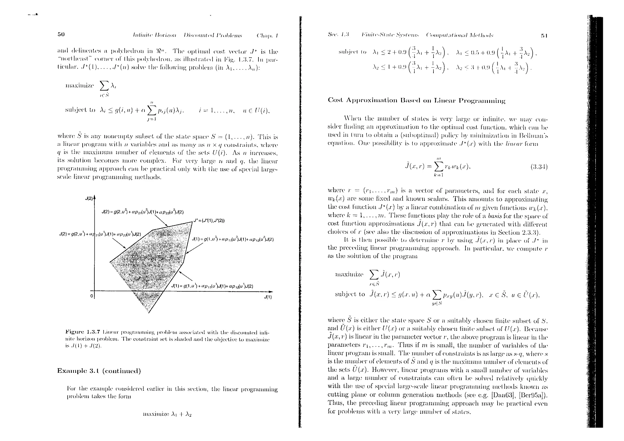
Example 3.1 (Illustration of the Error Bounds)
Consider a problem where there are two states and two controls
.S — {1.2),	(' -{ и 1. и “}.
The transition probabilities corresponding to the controls n1 and u2 are as
shown in log. 1.3.1: that is, the transition probability matrices are
'The transition costs are
.7(1. n1) = 2.	.7(1, i/2) =t)..r>,	.1/(2, a1) =1,	</(2, ii2) = 3,
and the discount factor is n = 0.9. The mapping 7’ is given for i = 1,2 by
{2	2	>
7(i, и1) -I- о y^/>o(»')70’). .</('', ч2) + <‘52ро(и2).1(.7) 7 •
j ।	j-i	J
The scalars c,. and сд of Eqs. (3.5) and (3.6) are given by
iiiiu{(7’*./)()) - (7’* './)(!), (T\/)(2) - (Ta'“'./)(2)},
e, n ma.x{(7’l./)(l) - (Tk 1./)(!), (7’‘ ,/)(2) - (7’A ~ 1 ./)(2)}.
The results of the value iteration met hod starting with the zero function ,/u
[./,,(1) = ./,,(2) = 0] are shown in Pig. 1.3.2 and illustrate the power of the
error bounds.
Sec. 1.3 Finite-State Systenis ( 'oiuput at/опа/ Met hod>
23
(a)	(b)
Figure 1.3.1 State transition diagram for Example 3.1: (а) и = a1; (b) и -- и'2
		(/’''•M (2)	+<.4	(7'М.Ю) +n-	+<lk	(T'U^CZ) +</.-
0	I)	0				
1	0.500	1.000	5.000	9.500	5.500	10.000
2	1.287	1.562	6.350	8.375	6 .(>25	8.650
3	1.811	2.220	6.856	7.767	7.232	8.1 11
4	2.414	2.745	7.129	7.540	7.160	7.870
5	2.896	3.247	7.232	7.417	7.583	7.768
6	3.343	3.686	7.287	7.371	7.629	7.712
7	3.741)	4.086	7.308	7.345	7.654	7.692
8	4.099	4.441	7.319	7.336	7.663	7.680
9	4.422	4.767	7.324	7.331	7.669	7.676
10	4.713	5.057	7.326	7.329	7.671	7.674
11	4.974	5.319	7.327	7.328	7.672	7.673
12	5.209	5.554	7.327	7.328	7.672	7.673
13	5.421	5.766	7.327	7.328	7.672	7.673
14	5.612	5.957	7.328	7.328	7.672	7.672
15	5.783	6.128	7.328	7.328	7.672	7.672
Figure 1.3.2 Peitoitii.iiicc ol (Ik* value item I i< >i i iix'lliod with and without the
error bounds of Prop, 3.1 for the problem of Example 3.1.
Termination Issues - Optimality of the Obtained Policy
Let us now discuss how to use the error bounds to obtain an optimal
-. .1
24	hdinit.c Horizon Discounted Problems Chiip. I
or near-optimal policy in a finite number of value iterations. We lirst note
that given any J, if we compute TJ ami a policy ц attaining the minimum
in I he calculation ol 7’./, i.e.. 7),./ — 7’.7, then we can obtain t.he following
bound on the siiboptimalily of /t:
max(7)—./*(/)] < - '‘(1- (ma.x[(7’.7)(z) - .7(/)] - inin[(7V)(/') - .7(7)]) .
(3.10)
To see this, apply Eq. (3.-1) with к = I to obtain for all i
Ct <./*(0- (7’./)(,) <e15
and also apply Eq. (3.1) with /r - I and with Tlt replacing T t.o obtain
c, </,,(/)- (7;,.7)(Z) = ./,,(/)- (LT.7)(7) < cq.
Subtracting the above two equations, we obtain the estimate (3.10).
la practice, one terminates the value iteration method when the dif-
ference (q. — q) of the error bounds becomes sufficiently small. One can
then Lake as linal estimate, of .!* the. “median”
or the “average”
II
Л = TkJ +	- £((7’A'•/)(/) - (T^'./)(7))e.	(3.12)
//,( 1 — n)
Both of these vectors lie in t.he region delineated by the error bounds. Then,
the estimate (3.10) provides a bound on the suboptimality of the policy p
at taining the minimum in t.he calculation of 7’A'.7.
The bound (3.10) can also be used to show that after a sufficiently
large number of value it ('rat ions, the st at ionary policy pA' that at tains the
minimum in t.he /rth value iteration [i.e. (7’ n7'A-l).7 = TA .7] is optimal.
Indeed, since the number of stationary policies is finite, there exists un
f > 0 such that if a st ationary policy )i satisfies
inax [./,,(/) - ./’(')] <
then // is optimal. Now let. /r be such that for all к > к we have
(max[(7’A./)W - (7* './)(/)] - nun [(7’A./)(,) - (7’A-‘./)(/)]) < c
Then from Eq. (3.10) we see that for all к > к, the stationary policy that
attains the minimum in the A'th value iteration is optimal.
See. 1.,'J l''imte-Stnto Systems Com[>iit.;itio:i;il Methods
25
Rate of Convergence
To analyze t lie rate о I con vergence of value i I era I ion with error bounds,
assume that there is a stationary policy //,* that attains the minimum over
fl in the relation
min Т1,'Г>‘~ 1 J — TkJ
lor all sufficiently large, so that eventually the met hod reduces to I lie
linear iteration
J : = fhi* + J-
In view of our preceding discussion, this is true for example if//* is a unique
optimal stationary policy. Generally t.he rate of convergence of linear itera-
tions is governed by the maximum eigenvalue modulus of the matrix of the
iteration [which is a in our case, sine/' any transition probability matrix has
a unit, eigenvalue with corresponding eigenvector c = (1,1,..., 1)'. while
all other eigenvalues lie within the unit, circle of t he complex plane).
It turns out, however, that when error bounds are used, the rat/'
at which the iterates .7/,. and .7,. of Eqs. (3.11) and (3.12) approach the
optimal cost vector J* is governed by the modulus of the subtlominanI
eigenvalue ol th/' transition probability matrix /)<•. that is. the eigenvalue
with second largest modulus. The proof of this is outlined in Exercise 1 .IS.
For a. sketch /if the ideas involved, let. Ai..... A„ 1 >/' the eigenvalues of
ordered according to decreasing modulus; that is
IM > |A2| >••> |A„|,
with A] equal to 1 ami A2 being t.he siibdominant eigenvalue. Assume that
there is a set of linearly independent. eigenvectors ci,/’2.e„ correspond-
ing to A|,A2...............................................A„ with с, = c — (1, 1... ., 1)'. Then th/' initial error
J — -7;1» can be expressed as a linear combination /if the eigenvectors
/ - •<,’ - £ I C T 52<jCj
j--2
for sonic scalars 41. £2,. . . .  Sim'/' 7),»./	//,,» -t-ol),*./ and --
Sis* +/'f',,» .7Z,». successive errors arc related by
T„»J =/!/>(./ -.7,,.), for all .1.
Thus t.he error after /,' iterations can be written as
II
J = 2
Using th/' error bounds/if Prop. 3.1 amounts to a. translation 01'7*../ along
the vector c. Thus, at best, th/' error bounds are tight enough to eliminate
the component ri*£t/’ of the error, but. cannot, affect t.he remaining term
ak Zq=2 A*'$//’j, 'vhi/'h diminishes like <ia'|A2|a' with A> being the stibdom-
inant eigenvalue.
luliiiite Horizon DHionnted I’roblonis C'hiip. 1
Л
26
Problems where Convergence is Slow
In Example 3.1, the convergence ol' value iteration with tin» error
bounds is very fast. For this example, it can be verified that //*(1) = »2,
/Г (2) = id , and that
/1/4 3/4 \
W 1/4 /
The eigenvalues of //,* can be calculated to be A| = 1 and A2 = which
explains the fast convergence1, since the modulus 1/2 of the subdominant
eigenvalue A2 is considerably smaller than ones On the other hand, there
arc situations where convergence of the method even with the use of error
bounds is very slow. For example, suppose that Pfl* is block diagonal with
two or more blocks, or more generally, that //,• corresponds to a system
with more than one (('current class of state's (see Appendix D of Vol. 1).
Then it can be shown that, the subdominant eigenvalue A2 is equal to I,
and convergence it typically slow when <1 is close' l.o 1.
As an example, consider tin' following three simple deterministic prob-
lems, each having a single policy and more' than one recurrent class of
states:
Problem 1: 11 --3, P,, = t hrce-dimensional ident ity, <;(/,//.(«)) = i.
I’ 10I1I.1111. 2: 11 — Г>. // = live-dimensional ident ity. </(/,/;(/’)) = i.
Problrm 11 — (>, </(/’,/1(1)) -- i and
/1	0	0	0	0	()\
0	0	1	0	0	0
_ 0	1	0	0	0	0
'' ~	0 0 0 Old 
0	0	0	0	0	1
\()	0	0	10	0/
Figure 1.3.3 shows the number of iterations needed by the value it-
eration method with and without the error bounds of Prop. 3.1 to find J,,
wit hin an error per coordinate of less than or equal to 10~G max;
The starting function in all cases was taken to be zero. The performance
is rather unsatisfactory but, nonetheless, is typical of situations where
the subdominant eigenvalue modulus of the optimal transition probabil-
ity matrix is close to 1. One possible approach to improve the performance
of value iteration for such problems is based on the adaptive aggregation
method to be discussed in Section 1.3.3.
Sec. 1.3 ldni(e-Sl<i(e Systems ( *<>liipu(;H ioiifd Mel hods
	Pr. 1 о .9	Pr. 1 о = .99	Pr. 2 о .9	Pr. 2 о .99	Pr. 3 о - .9	Pr. 3 о .99
W/out bounds	131	1371	131	1371	132	1392
With bounds	127	1333	129	1352	131	1371
Figure 1.3.3 Nunibrr of it era t ions for t he value it erat ion met he к I with mid with-
out error bounds. The problems arc deterministic. Because' the siibdoiiiinaiit
eigenvalue of the I ransit ion probability matrix is equal to 1, the error bounds are
inclfect ive.
Elimination of Nouopt,iinal Actions in Value Iteration
We know from Prop. 2.3 that,, il ft £ I7(i) is such that
<7(t. ft) + о ^2p,;(f/)J*0) > 7*(1).
J-1
then ft cannot be optimal at state /; that is, for every optimal stationary
policy /(, we have //.(/) yf ft. Therefore, if we are sure that the above
inequality holds, we can safely eliminate ft from the admissible set U(i).
While we cannot check this inequality, since we do not know the optimal
cost function ,7*. we can guarantee that it holds if
</(i. ii) + о ^21>ij(.ii)d.(.j) > J(i).	(3.13)
j = i
where 7 and 7 are upper and lower bounds satisfying
7(i)<7*(i)<7(0.	/ = 1....»
The preceding observation is the basis for a useful application of the
error bounds given earlier in Prop. 3.1. As these bounds arc computed
in the course of the value iteration method, the inequality (3.13) can be
simultaneously checked and nonopt,iinal actions can be eliminated from the
admissible set with attendant savings in subsequent computations. Since’
the upper and lower bound functions .7 ami 7 converge to J*, it can be seen
[taking into account the finiteness of the const raint set U(/)] t hat event ually
all nonopt,iinal fi £ U(i) will be eliminated, I,hereby reducing the set, U(i)
after a finite number of iterations to the set of controls that are optimal at
i. In this manner the computational requirements of value iteration can lie
substantially reduced. However, t he amount, of computer memory required
to maintain the set of controls not as yet eliminated at each i E S may be
increased.
28
lillinite Idiii/Ain Discounted I’mldeins C'hap. I
..ж
Gauss-Seidel Version of Value Iteration
In the value iteration method described earlier, the estimate ol' t.he
cost function is iterated for all states simultaneously. An alternative is to
iterate one state at a time, while incorporating into the computation the
interim results. This corresponds to using what is known as the Guus.s-
Si idcl. niclli.od. lor solving the nonlinear system ol equations J - I'd (see
[BeT8!)a] or [OrR7(l]).
For mdimensional vectors define the mapping F by
(/'•/)(!)
(3.1 1)
and, for i = 2,. . ., n,
(/<’./)(/)= min </(«, u) + пУ/!,i(ii.)(FJ)(j) + <> ^2/»,.;(«)•/(.;) 
In words, (/'’./)(/) is computed by the same equation as (7V)(i) except that
the previously calculated values (F./)(l),..., (FJ)(i — 1) are used in place
of ./(1),...../(/ - 1). Note that the computation of FJ is as easy as the
computation oiT.J (unless a. parallel computer is used, in which case the
computation of 7’./ may potentially be obtained much faster than FJ; see
[TsiSO], [BeTIJla] for a. comparative analysis).
Consider now the value iteration method whereby we compute J, FJ,
F2J,.... The following propositions show that the method is valid and
provide an indication of better performance over the earlier value iteration
method.
Proposition 3.2: Let J, J' be two n-diinensional vectors. Then for
any k — 0, 1,...,
max|(FM)(i) — (Fk J')(i)| < <ifc max| J(i) — J'(i)|.	(3.16)
Furthermore, we have
(FJ‘)(i) = J*(i), i G 5,	(3.17)
lim (FF/)(i) = J‘(i), i€ S.	(3.18)
Sec. I..'I
I'inili'-State S\^Iciiis	iniiel M<-llnxl>
2!)
Proof: It is sullicient to prove Eq. (3.16) lor Л- — 1. We have by the
definition of /’ and Prop. 2.4,
|(F./)(1)-(E.7')(1)| y. <i iimx|./(/) - ,/'(/)|.
Also, using this inequality.
|(F./)(2) -(FJ’)(2)\ -o.nax{|(F,/)(l) - (/’./')( I )|. |./(2) - ,/'(2)|.
И")
< о inax|.7(/) - J'(r)|.
Proceeding similarly, we have, for every i and j < i,
|(A./)(j) - U</')(j)| < a imix|./(t) - ./'(')!
so Eq. (3.16) is proved for к = 1. The equation FJ* = /* follows from the
definition (3.14) and (3.15) of F, and Bellman’s equation J* = TJ*. The
convergence property (3.18) follows from Eqs. (3.16) and (3.17). Q.E.D.
Proposition 3.3: If an n-diiuensional vector ./ satisfies
J(<) < (rJ)(i) < г =
then
(T‘ J)(j) < (FV)(i) < J*(i), z = l,...,n, /,:=!,2,... (3.19)
Proof: The proof follows by using the definition (3.14) and (3.15) of F.
and the monotonicity property of T (Lemma 1.1). Q.E.D.
The preceding proposition provides the main motivation for employ-
ing the mapping F in place of T in the value iteration method. The result
indicates that the Clauss-Seidel version converges faster than the ordinary
value iteration method. The faster convergence property can be substan-
tiated by further analysis (see e.g., [BeTSfla]) and has been confirmed in
practice through extensive experimentation. This comparison is somewhat
misleading, however, because the ordinary method will normally be used
in conjunction with the error bounds of Prop. 3.1. One may also employ
error bounds in the Clauss-Seidel version (see Exercise 1.9). However, there
is no clear superiority of one met hod over the ot her when bounds are in-
troduced. Furthermore, the ordinary method is better suited for parallel
computation than the Clauss-Seidel version.
30	Infinite Horizon Di^eounl<></ I’robleins ('hap. I
We note that, there is a more flexible form of the Clauss-Seidel method,
which selects states in arbitrary order to update I heir costs. 1'liis met hod
maintains an approximation ./ to the optimal vector .)*. and at each itera-
tion. it. selects a. state i and replaces ./(/) by (T.7)(i). The remaining values
•/(./), 1 И1 b are left unchanged. The choice of the state i at each iteration
is arbitrary, except for the restriction that, all slates are selected infinitely
often. This method is an example of an ii.si/ii<'liroiion..s Ji.re.il point iteration.
and can be shown to converge to .7* starting from any initial .7. Analyses
of this type of mid,hod are given in [Ber82a], and in Chapter 6 of [BeT8f)a]:
see also Exercise 1.15.
Generic Rank-One Corrections
We may view value iteration coupled with t he error bounds of Prop.
.3.1 as a method that makes a correction to the result.» of value iteration
along the unit vector c. It is possible to generalize the idea of correction
along a fixed vector so that it works for any type of convergent linear
iteral ion.
Let us consider the case of a single st ationary policy /i and an iteration
of the form J	I'.l, where
./ = II/, + Qii.l-
Here, Qt, is a matrix with eigenvalues strictly within the unit circle, and
/у, is a vector such that
•/„ =
An example is the Gauss-Seidel iteration of Section 1.3.1, and some other
(examples are given in Exercises 1.4, 1.5, and 1.7, and in Section 5.3. Also,
the value iteration method lor stochastic shortest path problems and a
single stationary policy, to be discussed in Section 2.2, is of the above
form.
Consider in place of .7 := an iteration of the form
.7 := I'.l,
where .7 is related to .7 by
.7 = .7 + yd.
with tl a fixed vector and у a scalar to be selected in some optimal manner.
In particular, consider choosing 7 by minimizing over 7
j|./ + 7d - I'V + 7<0If"-
which, by denoting
Sec. 1.3 b'initi'-St nt c Systems ('inninitiil iolinl Mel hods
31
can be written as
||./- К/ I Э(</ -.)|p.
By setting to zero tlie derivative of this expression with respect to * . it is
straightforward to verify that the optimal solution is
- --)'(/'•/ - •')
Thus the iteration J := IM can lie written as
./ := MJ.
where
MJ = IM + §c.
We note that this iteration requires only slightly more computation than
the iteration J := IM. since the' vector z is computed once and the com-
putation of у is simple.
A key question of course is under what circumstances the iterat ion
J := MJ converges faster than the iteration J := IM, and whether indeed
it converges at all t.o Jf,. It, is straightforward I,о verify t hat, in the case
where Qt, = o/’;, and </ — c, the it,oration J := MJ can be written as
!1
[compare with Eq. (3.12)]. Thus in this case the iteration J := d/(./) shifts
the result TltJ of value iteration to a vector that, lies somewhere in tin'
middle of the error bound range given by Prop. 3.1. By the result of this
proposit ion it. follows that t he iteration converges I,о
Generally, however, the iteration J MJ need not converge in the
case where the direction vector d is chosen arbit rarily. If on t he other hand
d is chosen to be an eigenvector of Qt,, convergence can be proved. This
is shown in Exercise 1.8, where it is also proved t hat, if d is tin. eigen w-
tor eoirespondiny Io the dominant ci.geimii.lue of Qt, (the. one. with. largest
modulus), the convcrgen.ee, rate of the iteration. J := A/J is governed by the
subdominant. eigenvalue ofQ,, (the one with, second, largest niotltilus). One
possibility for finding approximately such an eigenvector is to apply F a
sufficiently large number of times to a vector J. In particular, suppose that
the initial error J — can be decomposed as
tt
7 ~ 'hi ~	. Sj' .i
J=1
for some scalars .......f,,. where c,.....c„ are eigenvectors of Q,,. and
Ai,...,A„ are corresponding eigenvalues. Suppose also that Ai is the
32
Inlinilc Horizon Discounted Problems ('hnp. I
-Ж
unique dominant eigenvalue, that is, |A;| < |Ai| for j = 2,..., n. Then
the difference Fk+[,l — ]<’>.,/ is nearly equal to £1 (A,4 ' - A,)ci for huge к
and can be used to estimate the dominant eigenvector ci. In order to decide
whether к lias been chosen large enough, one can test to see if I,he angle
between the successive dillerenees 1 1,! — Fk J and Fk J - /'* 1 J is very
small; if this is so, the components of Fk+l.J — FkJ along the eigenvectors
<2.....c„ must also be very small. (For a. more sophisticated version of
t his argument., see [Ber93], where the generic rank-one correct,ion method
is developed in more general form.)
We can thus consider a two-pha.se approach: in the’ first phase, we
apply several times the regular iteration .7 := F.J both to improve our esti-
mate of ,7 and also to obtain an est imate d of an eigenvector corresponding
to a dominant eigenvalue; in the second phase we use the modified iterat ion
.7 := hl.I that involves extrapolation along </. it can be shown that the
two-pha.se method converges to ,7/, provided the error in t.he estimation of
d is small enough, that is, t.he cosine of t.he angle between d and Q^d as
measured by the ratio
(/‘47 _	-i,/)'( Fk~ i J - Fk~-O)
j|/47 - 7-A-1 ,/||  ||7^~1 (.7) -	-2,/||
is sufficiently close to one.
Not.i't hat the computation of the first phase is not wasted since it uses
the iteration J : = F.J that we are trying to accelerate. Furthermore, since
the second phase involves the calculation of F.J at the current iterate .7, any
error bounds or termination criteria based on F.J can be used to terminate
the algorithm. As a result, the. same Unite termination mechanism can be
used for both iterations J := F.J and .7 : = hid.
One difficulty of the correction method outlined above is that the
appropriate vector d depends on and therefore also on /;. In the case
of optimization over several policies, the mapping F is defined by
г
II
(F./)(i) = min //,(//) +	</o(")'7(./)
J- I
1 = 1,..., n. (3.20)
One can then use the rank-one correction approach in two different ways:
(1) Iteratively compute the cost vectors of the policies generated by a
policy iteration scheme of the type discussed in the next subsection.
(2) Guess at an opt imal policy within the first phase, switch to the second
phase, and then return to the first phase if the policy changes “sub-
stantially’' during the second phase. In particular, in the first phase,
t.he iteration .7 := F.J is used, where F is the nonlinear mapping of
Eq. (3.20). Upon switching to the second phase, the vector z is taken
Sec.. 1.3
I'init e-St ;it < Systems ( \ >ni{ nil-it i< ni;il McIIhhS
33
to be equal to where //,* is the policy that attains the minimum
in Eq. (3.2(1) at the time ol the switch. The second phase consists ol
the it era! ion
.1 = MJ = /<’,/ + уг,
where /•’ is the nonlinear mapping of Eq. (3.20), and / is again given
by
To guard against subsequent changes in policy, which induce cor-
responding changes in the matrix Q,,», one should ensure that the
method is working properly, for example, by recomputing </ if the
policy changes and/or the error Ц7Л/ — ,/|| is not reduced at a sat-
isfactory rate. This method is generally effective because the value
iterat ion met hod typically finds an opt imal policy much before it. finds
t he optimal cost vector.
It should be mentioned, however, that the rank-one correction method
is ineffective, if there is little or no separation between the dominant, and
the subdoininant eigenvalue moduli, both because the convergence rate of
the method for obt aining d is slow, and also because the convergence rate
of the modified iteration .7 M.J is not much faster than the one of th<'
regular iteration .7 := b'J. For such problems, one should try corrections
over subspaces of dimension larger than one (see [Ber!)3], and the adaptive
aggregation anil multiple-rank correction methods given in Section 1.3.3).
Infinite State Space — Approximate Value Iteration
The value iteration method is valid under the assumptions of Prop.
2.1, so it is guaranteed to converge t.o .7* for problems with infinite state
and control spaces. However, for such problems, the method may be im-
plementable only through approximations. In particular, given a function
.7, one may only be able to calculate a function .7 such that
(3.21)
where f is a given positive scalar. A similar situation may occur even
when the state space is Unite but the number of states is very large, d’hen
instead of calculat ing (7’./)(.r) for all stales .r, one may do so only for some
states and est imate (7’./)(.i.') for t he remaining states .i: by some form of
interpolation, or by a least-squares error lit. of (T.7)(.r) with a. fimetion
from a suitable parametric class (compare with t.he discussion of Sect ion
2.3). Then the function -7 thus obtained will satisfy a relation such as
(3.21).
inax|./(.r) - (T./)(.r)| < r,
.. .ж
3d	hiliiiilf Ihni.'ott I yisct unit id PrttltlvHix С’/ьч/,. /
We are thus led to consider the approximate value iteration method
that generates a sequence {.//. } satisfying
uiax|.4+1(.r)-(T.4)(.r)| <<.	/, = 0,1,...	(3.22)
starting from an arbitrary bounded function ./(). Generally, such a sequence
“converges” to ./* to within an error of</(l - o). To see this, note that,
Eq. (3.22) yields
— re < Ji < /'./a + re.
By applying 7 to this relation, we obtain
T-Jo — orc < TJi < T2.Jy + nrc,
so l>y using Eq. (3.22) to write
7’./| - <<’ < .1-2 < 7 -/| I <<’
we have
T2.!» - c(l + o)c < -h < T2J„ + f(1 + a)e.
Proceeding similarly, we obtain for all A' > 1,
7’A ’ 1 Jo — <-( 1 + о +  • • + oA'~1 )c < Jk < 7’A - 1 •/(> + r(l + a +    T <P'_ ')e.
By taking the limit, superior and I,he limit, inferior as к -  oo, and by using
the fact, linu—cv 7’A'./() = ./*, we see t hat,
./*--------< < lim inf .4- < limsup.4 < .!* 3------—c.
1 - Г1	A' = oc	1 — О
It, is also possible to obtain versions of the error bounds of Prop. 3.1
for the approximate value iteration met hod. We have from that proposit ion
7’./*- -	min[(7'.4)(.r)-.4(.r)]e<./*
< Г,,к +	1^[(7’Л)(.г) - ./д (.г)]с.
By using Eq. (3.22) in the above relation, we obtain
• 4l 1 - К' -	— min [.//,. + 1 (.r) + < - /*(./•)]<' < ./*
1 — О .rf=.S L	J
< л ( I + cc + -t-n iiia,x[j/,_H(.'r) + f - Jk(./:)]c,
1 — H zG.S' L	J
or
<+a min.,.G.s-[./A..H(.r) - .//.-(.г)|
/. . . - _____________L_____________-‘ , I *
( d-rimax.,.(-.s [.//.-g । (.f) - .4(;r)]	i
< -4 i i 3---------------------7-------------------c.
I - о	>
These bounds hold even when the state space is infinite because the bounds	|
of Prop. 3.1 can be shown for an infinite' state space as well. However, for	f
these bounds to be useful, one should know r.
1.3.2 Policy Iteration
The policy iteration algorithm generates a sequence of stationary poli-
cies, each with improved cost, over the preceding one. Given the station-
ary policy //, and the corresponding cost function an improved policy
{/7,//,...} is computed I>y minimization in the DI’equation corresponding
to Jfl. that is. T-fi.l,, = T./p. and the process is repeated.
The algorithm is based on the’ following proposition.
Proposition 3.4: Let p, and //, be stationary policies such that. T^Jtl =
or equivalently, for i = 1,..., n,
II	II
з(г,7*(г))+о ^7^(Д(г))./л0) = min v(i, u) + о. V (а)./л(у) .
7=1	L	j=i
Then we have
4(0 <	(3.23)
Furthermore, if /1 is not optimal, strict inequality holds in the above
equation for at least one state i.
Proof: Since J/z = (Cor. 2.2.1) and, by hypothesis. = T.)ti. we
have for every /.
M') = .'/('•//(/)) + 0	,(//.(/))./,,(.;)
j-1
= (Зд(')-
Applying repeatedly on both sides of this inequality and using t he mono-
tonicity of 1- (Lemma 1.1) and Cor. 2.1.1, we obtain
> /pdp >  • • > ГЗ •/,, >    > Jii 11^ l~ /,, = •//,.
proving Eq. (3.23).
If ./,, -- ./77, then from the preceding relation it. follows that -
Tj7.7;, and since by hypothesis we have TjjJii = 77/p., we obtain = T.Jf,.
implying that ,/z, = ./* by Prop. 2.2. Thus // must, be optimal. It. follows
that if /I is not optimal, then	for some st.ate i. Q.E.D.
36	luliiiitt' llori/.on I )i.s<4 unit c< I	('h.q>. I
Policy Iteration Algorithm
Step 1: (Initialization) Guess an initial stationary policy /z°.
Step 2: (Policy Evaluation) Given the stationary policy /zA:, com-
pute the corresponding cost function J k from the linear system of
equations
(/ - o/',fc)J/lfc = (i^-
Step 3: (Policy Improvement) Obtain a new stationary policy
Hk+l satisfying
1J .,k — T J ,,k.
If ,lflk = stop; else return to Step 2 and repeat the process.
Since the collection of all stationary policies is finite (by the finite-
ness of S and O') and an improved policy is generated at every iteration,
it follows that the algorithm will find an optimal stationary policy in a
finite number of iterations. This property is the main advantage of pol-
icy iteration over value iteration, which in general converges in an infinite
number of iterations. On the other hand, finding the exact value of Jr
in Step 2 of the algorithm requires solving the system of linear equations
(I —	The dimension of this system is equal to the num-
ber of st.ates, and thus when this number is very large, the method is not
attractive.
Figure 1.3.4 provides a geometric interpretation of policy iteration
and compares it with value iteration.
We note that in some cases, one can exploit the special structure of
the problem at, hand to accelerate policy iteration. For example, sometimes
we can show that if /(. belongs to some restricted subset Л/ of admissible
control functions, then ,//t has a. form guaranteeing that /7 will also belong
to the subset ЛЛ In this case, policy iteration will be confined within
the subset Л/. if the initial policy belongs to Л/. Furthermore, the policy
evaluation step may be facilitated. For an example, see Exercise 1.14.
We now demonstrate policy it,erat ion by means of the example con-
sidered earlier in this section.
Example 3.1 (continued)
Let us go through the calculations of the policy iteration method:
Initialization: We select, the initial stationary policy
111 i >	I	< J /1\	‘2
/'• (1) = и. ,	/I. (2) = и .
Sec. /.3
I'initc Xlttle Xyslriiis (‘t ни/>ut .it it >11.1/ Melhtitl.'-
37
Figure 1.3.4 Geometric interpretation of policy iteration and value iteration.
Each stationary policy /1 defines the linear function <ifl I- счРц.1 of the vector ./.
and TJ is the piecewise linear function min/([<//f 4 о/p./]. The optimal cost ./*
satisfies J* = TJ*. so it is obtained from the intersection of the graph of TJ and
the 45 degree line shown. The value iteration sequence is indicated in the top
figure by the staircase construction, which asymptotically leads to J*. The policy
iteration sequence terminates when the correct linear segment of the graph nfTJ
(i.e., the optimal stationary policy) is identified, as shown in the bottom figure.
38
bilinite I lori/.on	I )ixci >i 11 it < •• 1 Problems (7iap. I
.. «ж
Policy Evaluation: We obtain Jfio through the equation J/(o = 7’о J о or.
equivalent ly, the linear system of equal ions
Лз'О) =	+ <ipn("' i) + opi-iG?(2).
-/,,<>(2) = '/('Л"2) + op-2i (a2)-/,,<>( 1) + np22(«2)-/,,i>(2).
Substituting the data of the problem, we have
./ ,,(1) = 2 t 0.9- ~  ./„(I) + 0.9  1  ./ »(2),
1	I
./„„(2) = 3 + 0.9 - 1 I) + 0.9 	(2).
Solving this system of linear ('({nations for ♦/,<(!) and .//to(2), we obtain
,//(o(l) — 21.12,	,/?t(2) -25.9G.
Policy Improvement: We now lind /л1 (I) and p’(2) satisfying 7‘ ।./ (l —
T,) n. We have
(7'.//,0)(l) = inin 12 + 0.9	• 21.12 + j  25.96
0.5+ 0.9	-21.12 + -25.9(1)
= iniii{24.12,23.45} = 23.45,
(7’./p0)( 1) = mi" < 1 + 0.9	• 24.12 +  25.96
3 + 0.9
21.12 + ~ -25.96
4
= inin{2.3.12, 25.95} = 23.12.
4’110 minimizing controls are
/,1(0 = „Л //(2) = n'.
Policy Evaluation: We obtain ./(1i through the equation ./^i —
(>) = .'/(I - »2) + «Pi i("2)-/„। (0 + '1/Л2(«2)-У i (2),
ЛЯ1) = -'/(‘Л "') + пр-т (»')•/,,! (1) + op22(u')-/;,i(2).
See. i.:{
riuite-St:ile Systems ( 'tmijmt :it i<mill Mctlunls
3!»
Substitution of tho data of the problem and solution of the system of equal ions
yields
, i (11 ~ 7.3.3,	,/(i i (2) ~ 7.67.
Policy Improvement: We perform the minimization required to lied 7'7 j :
)(1) = min
 7.33 +
= miu{3.67, 7.33} =
7.33,
(T7pl )(2) = min
1
4
lienee we have 7 t = T.l i . which implies that p.1 is optimal and 7 । — J':
//*(!) = a2, p*(2) = u',	7*(1)~7.33,
Modified Policy Iteration
When the number of states is large, .solving the linear system (/ —
aP^i. ).f к = U^k in the policy evaluation step I >y direct methods such as
Gaussian elimination can be prohibitively time-consuming. One way to
get around this difficulty is to solve the linear system iteratively by using
value iteration. In fact, we may consider solving the system only approx-
imately by executing a limited number of value iterations. This is called
the modijied policy deration olyorithni.
To formalize this method, let Jo be an arbitrary //.-dimensional vector.
Let ttii.    be positive integers, and let the vectors ,I\. .h,. . . and the
stationary policies po. p.j. ... be defined by
T^.lk -T./k,	-h. (l -T’^./k. h (I. I,--.
Thus, a stationary policy /А is defined from -h. according to T k.Jk = TJk-
and t.he cost. J к is approximately evaluated by ntk — 1 a<Iditioilai value
iterations, yielding the vector ,Jk । |. which is used in turn to define /Л1 1.
We have the following:
40
InliiiHe Horizon Discounted Problems
Chap. 1
Proposition 3.5: Let {./»,} and {/nJ; be the sequences generated by
the modified policy iteration algorithm. Then {J^} converges to J’.
Furthermore, there exists an integer к such that for all к > к, /Л is
optimal.
Proof: Let r be a scalar such that the vector Jo, defined by Jo = Jo + re,
satisfies TJo < Jo- [Any scalar г such that max, [(TJo)(?) — Jo(/)] <
(I <i)r lias this property.] Define lor all k. Jk\ i 7’/,”1 J*. Then, it can
be seen by induction that for all к and m = 0,1,. . ., m/,, t.he vectors T”'k.Jk
and dilfer by t he multiple of t.he unit vector co"'0 1 " 1 "'l 1 и"с. It,
follows that if Jo is replaced by Jo as the starting vector in I he algorithm,
the same sequence of policies {///. } will be obtained; that is, wo have for all
k
T^Jr^TJ,..
Now we will show that for all к we have- < 7VJU. Indeed, we have
T и Jo = 7’Jo < Jo, from which we obtain
;u = l,2,...
so that.
7>7, = TJt < Tfl„Ji = 7’;;'” H7o < 7;7Jo = 'Jx < TtloJo = TJo.
This argument can be continued to show that for all k, we have J/, <
T-h. i, so that
7a- <7’<7o, A: = 0,1,...
On the other hand, since TJo < Jo, we have J’ < Jo, and it, follows
that application of any number of mappings ol the iorm 7], to Jo produces
functions that are bounded from below by .T. Vlllis.
7 • J... a-= 0.1....
By taking the limit as A' -e -x. we obtain lim/,. . x •/;, ('/ = J'(') h>r '•
.md since Inn,, . x <T, Л '	(1. we obtain
^liin Ji,(i) = J‘('l, i ~ 1....."
Since the number of stationary policies is finite, there exists an T > 0
such that if a stationary policy // satislies
max[j,,(/) - J*(t)] < Г.
Sec. I..'l	e-St.m<• .Systems Computational Methods
11
then ц is optimal. Now let A’ be such that lor all k > k we have
j£~ (niax[(7'.A-)(/) .A-(')] nun [(7’.A-)(') -A-(0])-'-
Then from Eq. (3.10) we see that for all A' > A’, the stationary policy fik'
that satisfies T k.Jk = 7’-A- is optimal. Q.E.D.
Note that if ntr = 1 lor all A' in the modified policy it erat ion algoril Inn,
wc obtain the value iteration method, while if пц. — oo we obtain the policy
iteration met hod. where the policy evaluation step is performed iteratively
by means of value iteration. Analysis and computational experience suggest
that it is usually best, to take /»/.. larger t han 1 according t.o some heuristic
scheme.. A key idea here; is that, a value iteration involving a single policy
(evaluating 7),,/ for some //. and ./) is much less expensive than an iteration
involving all policies (evaluating 7'./ for some ./), when the number of
controls available at each state is large. Note that error bounds such as
the ones of Prop. 3.1 can be used to improve the approximation process.
Furthermore., Gauss-Seidel iterations can be used in place of the usual value
iterations.
Infinite State Space - Approximate Policy Iteration
The policy iteration method can be defined for problems with infinite
state and control spaces by means of the relation
T к i i •/. *- = T.1 к, A: = 0 1,....
The proof of Prop. 3.4 can then be used to show that the generated se-
quence of policies {/?•'} is improving in the sense that, J i < ./,* for all
k. However, for infinite state- space problems, I,he policy evaluation step
and/or the policy improvement step of the method may be implementable
only through approximations. A similar situation may occur even when
the state space is finite but, the number of states is very large.
We arc thus led to consider an approximate policy iteration method
that generates a sequence of stationary policies {//*} and a corresponding
sequence of approximate cost functions {.A } satisfying
max |./A,(.r)-./A.(.r)|< A k = 0,1,...	(3.2-1)
.r 6 5	t
and
max I(7)p_> J;,- )(.r) - (7.A. )(z )| A <.	к - l>. 1... .	(3.2'i)
where b and t are some positive scalars, and //’ is an arbitrary station-
ary policy. We call this the (ippro.fimate policy iteration algorithm. The
following proposition provides error bounds for this algorithm.
42
Infinite Hori/.on Di.sconnl.ed Problems ('hup. /
..Il
Proposition 3.6: The sequence {/ik} generated by the approximate
policy iteration algorithm satisfies
lim sup max
c + 2nd
(1 — a)2
(3.26)
Proof: Krom Eqs. (3.24) and (3.25), we have for all
7z,n i ./;p - <n*»c < T/(hi -Л- < 'l .Jk +
where c = (1, 1,. . . , 1)' is the unit vector, while from Eq. (3.21), we have
for all /.•
7’./;, < 7’./;p 4- tide.
By combining these two relations, we obtain for all /,
I '•/,/ - 77/zd + (' + 2оЛ)с < T^-1,,1. h (< 4- 2o<*>)c.	(3.27)
1'i'oni Eq. (3.27) and the equation T^/,,1 t = ./pZ. , we have
7’p t i a <	+ (< + 2od)c.
By subtracting from this relation the equation 7’p-n Jp + i = -/^a+i, we
obtain
7'(/- I I .//(A- — 7,,A t 1 ./;|A t 1 < .//(A- — 7,рч-1 + (< + 2(ld)c,
which can be writ ten as
-//(a t i - 7zp- < <>/'), + (< + 2<id)e,	(3.23)
where l‘\ is the function given by
= (>-l(7;p, ,./„,,+ 1)(.r) - o-- '(7>U./,p.)W
= E{,/;p +, (/ (,r,	1 (,r),»’)) — (J U /'A +1 ('-’) , "')) } 
Let.
Then we have 7). (,r) <	f”1' all .r C .S’, and Eq. (.3.28) yields
0,- < o£a- i- < I- 2<>л,
Sec. 1.3
Finite-Stale Systems C'cin/iut;il ioicil Methods
Let
<* = ('') ~ 7 "(•'))
From Eq. (3.27) and I lie relation
~ 7*W) <
which follows from Prop. 2.1, we have
T)p. ( । .l^k < T.l^. + (< + 2oh)c <	4- aCy 4 (< 4 2<u'i)c.
We also have
7),n । ./(p. —	1 i + 7’zjo i ./;1r - 7’p-.( । Jfy4 ।.
and by subtracting the last two relations, we obtain
- •/’ < (i(j. + <il'\ 4 (< 4 2oh)c,
From this relation we see that
Ц-П < <"<A- + «ЧА- 4 f + 2nd.
By taking tlit- liinit superior as к -e oc and by using Eq. (3.29), we obtain
г + 2аЛ
(1 - о) lim sup 0,. < о---------1< + 2nd.
A—ex.	1 - <i
This relation simplifies to
..	t + 2оЛ
Inn sup < T.--------ex.
A-.oo (1— rl)‘
which was to be proved. Q.E.D.
Proposition 3.6 suggests that, the approximate policy it,orat ion met hod
makes steady progress up to a point and then the iterates ./ t oscillate
wit,hili a neighborhood of the optimum J*. This behavior appears to be
typical in practice. Note that for <*> = () and < = 0, Prop. 3.6 shows that
the cost sequence {./pr} generated by t he (exact) policy iteration algorit hm
converges to J\ even when the state space is infinite.
-Ж
44	tntinite Horizon Discounted Problems CIui/i. 1
1,3.3 Adaptive Aggregation
Let. us now consider an alternative to value iteration for perform-
ing approximate evaluation of a stationary policy //., that is, for solving
approximately tin? system
Л' - /
Tins alternative is recommended for problems where convergence of value
iteration, even with error bounds, is very slow. The idea here is to solve
instead of t.he system	another system of smaller dimension,
which is obtained by lumping together the states of the original system
into subsets Si, S-2,.. ., Sm that can be viewed as aggregate states. These
subsets arc disjoint and cover the entire state space, that is,
5 = Si U S-> u   • и s„,.
Consider the n x m matrix 11' whose Zth column has unit entries at coor-
dinates corresponding to states in .S', and all other entries equal to zero.
Consider also an tn x n matrix Q such that tin: ith row of Q is a probability
distribution (</,, ,..., </,„) with qis = 0 if s (f S;. The st.ruct.uix: of Q implies
two useful properties:
(a)	QIT = I.
(b)	The matrix
S = QP„\V
is an in x in transition probability matrix. In particular, the i/th
component of П is equal to
D j = 52<iis 52
.s£.S',	lets J
and gives the probability that, the next, state will belong to aggregate
state S', given that t.he current state is drawn from the aggregate
stale S, according to the probability distribution {r/,.s | s E S’,}. The
transition probability matrix H delines a Markov chain, called the
aggregate Markon chain. whose stat.es arc the in aggregate states.
Kigurc 1.3.5 illustrates the aggregate Markov' chain.
Aggregate Markov chains are most useful when their transition be-
havior captures the broad attributes of the behavior of the original chain.
This is generally true if the slates of each aggregate state are “similar" in
some sense. Let us describe one such situation. In particular, suppose that
we have an estimate ./ of Jz, and (hat we postulate that over the slates s
of (’very aggregate stale Si the variation, ./,,(«) — J(.s) is constant. This
amounts to hypothesizing that for some m-dinicnsional vector g we have
=- IT//.
Sec. /..'J
I'i uile-St al <• S'v.steius C'i>m/iul;it i<in;il Met hulls
45
Figure 1.3.5 Illustration of the aggregate Markov chain. In this example, the
aggregate states are 5| — {1,2,3}, .S’2 — {-1,5}, and 5’,; = {(>}. The matrix 1Г
Ims-columns (I. 1, 1,(1,(),(>)', (0,0,0, 1, 1,0)', ami (0, 0, 0, 0, 0, 1)'. In this example,
the matrix Q is chosen so that each of its rows defines a nnilorni probability
distribution over the states of the corresponding aggregate state. Tillis the rows of
Q are (1/3, 1/3, 1/3,11,0,0), (0.0,0, 1/2, 1/2,0), and (0,0,0,11,0, 1). The aggregate
Markov chain lias transition probabilities rn = ^(/>21 + />23), ri2 - (pi t + Pal).
>'13 = 0. 1'21 = 5 (p.12 + Раз), r22 = 5/45. '"2.3 = .jPKi. ''31 = 0. '32 = Ц» and
143 = 0.
13y cotiillining t.he equations 7},.,/ = </,, + <i/’,.7 anil </(l = (7 — of},)./,,. we
have
(7= J.
This is the variational form of the equation = T^Jf, discussed earlier in
connection with error bounds in Section 1.3.1, and can be used equally well
for evaluating Let us multiply both sides with Q and use the equation
Jp — J = Wy. We obtain
which, by using the equations = I and R = Ql’^W. is written as
(J - o/?),i/ = Q(T„.J - ./).
This equation can be solved for y, since 7?. is a transition probability matrix
and therefore the matrix I — nR is invertible. Also, by applying 7}, t.o both
sides of the equation .7,, = ./ + Wy, we obtain
7/,. = 7},./;, = 7},./ 4 о//,11’//.
We thus conclude that, if the variation of — .7(.s) is roughly con-
stant over the states .s of each aggregate state, then the vector 7/,./-bo//, II'?/
is a good approximation for ./,,. Starting with ,/. this approximation is ob-
tained as follows.
_. .1
46	liilinite Hoii/Aiu D'lMOiuited I’roblvius ('biiy. I
Aggregation Iteration
Step 1: Compute 7}, J.
Step 2: Delineate the aggregate states (i.e., doline IV) and specify
tin: matrix Q.
Step 3: Solve fur у the system
(I -nI7)/y = (?(7’„./ - ./).	(3.30)
where R = QP^W, and approximate .Jt, using
.J := TltJ + nP.Wy.	(3.31)
Note that, the aggregation iteration (.3.31) can be equivalently written
as
./ :=7),(,7 + Il’/y),
so it. differs from a value iteration in that it. operates with Tt, on J -t- \Vy
rather than
Solving the system (3.30) in the aggregation iteration has an inter-
esting interpretation. It. can be seen that у is the o-discountcd cost vector
corresponding to tlie transition probability matrix R and the cost-per-stage
vector	— J). Thus, calculating у can be viewed as a policy evalua-
tion step for t.he aggregate Markov chain when the cost per stage for each
aggregate state .S’, is equal to
E<a.s((7;,j)W-./(.s)).
which is the average 7),./ — ./ over the aggregate state Si according to the
distribution | s fc S,}. A key attractive aspect of the aggregation
iteration is that t.he dimension of the system (3.30) is m (the number of
aggregate states), which can be much smaller than и (the dimension of the
system Jfl = arising in the* policy evaluation step of policy iteration).
Delineating the Aggregate States
A key issue is how to identify the aggregate states 5j,. .., 5',,, in a.
way t hat the error — ./ is of similar magnitude in each one. One way
to do this is to view 7),./ as an approximation to and to group together
states i with comparable magnitudes of (7'),.7)(i) — J(i). Thus the interval
[c.c], where
c = mm[(7),./)(/) - ./(/)], c = max[(’7|,./)(z) - J(z)],
Sec. I.:!
h'inite-Stiite Systems C'om/mt.nt iomd Methods
47
is divided into in segments and membership ol a slate / in an aggregate
state is determined by the segment within which (7),./)(/)	./(/) lies. By
this we mean that for each state i. we set i t Si if (7),./)(,) - ./(?) = c. and
we sot,
/ £ .S't. if (7),./)(/) - J(i) - <_• - (A- - Ф с (О, Л].
where
h =
III,
This choice is based on the conjecture that, al least near convergence.
(T;I./)(?) — ./(/) will be of comparable magnitude for states i for which
Jii(i) — ./(/) is of comparable magnitude. Analysis and experimentation
given in [BeC89] has shown that the preceding scheme often works well
with a small number of aggregates st.at.es in (say 3 to 6), although the
properties of the method are yet fullv understood.
Note that the aggregate states can change from one iteration to the
next, so the aggregation scheme “adapts’’ I,о the progress of the computa-
tion. The criterion used to delineate the aggregate states does not exploit
any special problem structure. In some cases, however, it is possible to take
advantage of existing special structure and modify accordingly the method
used to form the aggregate states.
Adaptive Aggregation Methods
It is possible to construct, a number of methods that calculate by
using aggregation iterations. One possibility is simply to perform a se-
quence of aggregation iterations using the preceding method to partition
the state space into a few, say 3 to 10, aggregate states. This method
can be greatly improved by interleaving each aggregation iteration with
multiple value iterations (applications of the mapping Tt, on the current it-
erate). This is recommended based on experimentation and analysis given
in [BeC’89], to which we refer for further discussion. Au interesting em-
pirically observed phenomenon is that the error between the iterate and
J/z is often increased by an aggregation iteration, but. then unusually large
improvements are made during the next few value iterations. This sug-
gests that the number of value iterations following an aggregation iterat ion
should be based on algorithmic progress: that is, an aggregation iteration
should be performed when the progress of the value iterations becomes rela-
tively small. Some experimentation may be needed with a given problem to
determine an appropriate criterion for switching from the value iterations
to an aggregation iteration.
Then1 is no proof of convergence of t he scheme just, described. On the
basis of computational experimentation, it appears reliable in practice. Its
convergence nonetheless can be guaranteed by introducing a feature that

48	lu/iiiife Horizon Discounted Problems Chap. 1
enforces some irreversible progress via t.he value iteration method following
an aggregation iteration. In particular, one may calculat.e the error bounds
of Prop. 3.1 at the value iteration Step 1, and impose a requirement that,
the subsequent, aggregation iteration is skipped if these error bounds do
not improve by a certain factor over the bounds computed prior to the
preceding aggregation iteration.
'Го illustrate the effectiveness of the adaptive aggregation method,
consider the three deterministic problems described earlier (cf. Pig. 1.3.3),
and the performance of the method with two, three, and four aggregate
states, starting from the zero function. The results, given in Pig. 1.3.G,
should be compared with those of Fig. 1.3.3.
It. is intuitively clear that the performance of the aggregation method
should improve as t he number of aggregate states increases, and indeed the
computational results bear this out. The two extreme cases where in = n
and in = 1 are of interest. When in — n, each aggregate state has a single
state and we obtain I he policy iteration algorithm. When ш = 1, there is
only one aggregate state, IT is equal to the unit vector c = (1,. . ., I)', and
a straight forward calculation shows (.hat. for the choice Q = (1/n, . . . , I//(),
the solution of the aggregate system (3.30) is
From this equation (using also the fact /),c — c), we obtain the iteration
’ := T"7 +	- •/(’))<	(3.32)
which is the same as the rank-one correction formula (3.12) obtained in
Section 1.3.1 and amounts to shifting the result Tz,7 of value iteration
within the error bound range given by Prop. 3.1. Thus we may view the
aggregation scheme as a. cont inuum of algorithms with policy iteration and
value iteration (coupled with t he error bounds of Prop. 3.1) included as the
two extreme special cases.
Adaptive Multiple-Rank Corrections
One may observe that, the aggregation iteration
I- II'//).
amounts to applying 7), to a correction of .) along the subspace spanned
by the columns of II’. Once the matrix II' is computed based on the adap-
tive procedure discussed above, we may consider choosing the vector ij in
alterant ive ways. An interest ing possibility, which letuls to a generalization
Sec. 1.3
I'inile-St-iit e Systems ( omputat ion;d Met hods
49
No. of aggregate states	I’r. 1 0 = .9	I’r. 1 0 = .99	I’r. 2 0 = .9	I’r. 2 0 = .99	I’r. 3 0 = .9	I’r. 3 0	.99
2	14	13	9	9	S3	505
3	1	1	3	3	61	367
1			3	3	26	351
Figure 1.3.6 Number of iterations of adaptive aggregation methods with two,
three, and Гонг aggregate slate's Io solve t he problems of b’ig. 1.3.3. Kach low ol
Q was chosen to define a uniform probability distribution over the states of the
corresponding aggregate stale.
of t.he rank-one correction method of the preceding subsection, is to select
у so that
\\./ + \Vy~Tl,(J + \\'y)\\2	(3.33)
is minimized. By setting to zero the gradient, with respect, to у of the above
expression, we can verify that the optimal vector is given by
v = (Z'Z)-'Z'(T/(,/-./),
where Z = (I — ng,)IV’. The corresponding iteration then becomes
J := g,(J + IF//) = T„.J + ng,IT//.
Much of our discussion regarding the rank-one correction method also
applies to this generalized version. In particular, we can use a. two-phase
implementation, which allows a return from phase two to phase one when-
ever the progress of phase two is unsatisfactory. Furthermore, a. version of
the method that works in the case of multiple policies is possible.
1.3.4 Linear Programming
Since lim,у —,TN.J = ./* for all .J (cf. Prop. 2.1), we have
.J <TJ =>	./<./* =T.J*.
Thus J* is the “largest” ./ that satisfies the constraint J < 7'./. 'This
constraint can be written as a finite system of linear inequalities
7(i) <</(/,«) +о ^2 p,, (a)./(7).	/=1....11.
50
liiliuilv llori/.oii Dixcounled Problems (-Imp. 1
and delineates a polyhedron in ')?". The optimal cost, vector J* is t.he
'northeast ' corner of this polyhedron, as illust rated in Fig. 1.3.7. In par-
ticular. •/*(!)....../*(/;) solve the following problem (in A,.........A„):
maximize A,
II
subject to A, < (j[i, u) + n	Il G Гф).
2=1
where S' is any nonempty subset of the state space S' = (!,..., n). This is
a linear program wit h /I variables and as many as /1 x q constraints, where
q is the maximum number of elements of t.he sets U[i). As n increases,
its solution becomes more complex. For very large n and q. the linear
programming approach can be practical only with the use of special large-
scale linear programming methods.
Figure 1.3.7 Linear programming problem associated with the discounted infi-
nite horizon problem. 'Che constraint set is shaded and the objective to maximize
is ./(!) + ./(2).
Example 3.t (continued)
For the example considered earlier in this section, the linear programming
problem takes t he form
maximize Ai + A,
S<-e. /.3
I' iiiil c-Sl:it e Systems	( '< mquil,/I u>n;il Melh<nls
51
subject to A, < 2 + 0.9 ( j z''1 + jA,
A2 < I + 0.9	+ p\2
A, < 0.5 + ().!) (--A, + ^A,
Aj < 3 I 0.9 (jAi 5 -’.vj
Cost Approximation Based on Linear Programming
When the number of slates is very large or infinite, we may con-
sider finding an approximation to the optimal cost, function, which can be
used in turn to obtain a (siiboptimal) policy by minimization in Bellman's
equation. One possibility is to approximate ./*(./) with the Ипсат form
III
r) =	(3.34)
A--1
where г = (/q......rin) is a vector of parameters, and for each state ,r,
шд.(.г) are some fixed and known scalars. This amounts to approximating
the cost function ,/*(./) by a linear combination of/// given functions //g.(.r),
where k = 1,. .., ///. These functions play t.he role of a basis for the space of
cost function approximations J(.r.r) that can be generated with different
choices of r (see also the discussion of approximations in Section 2.3.3).
It is then possible t.o determine r by using ./(./,/) in place of ./• in
the preceding linear programming approach. In particular, we compute /'
as the solution of the program
maximize ,/(./•, /)
.re.s
subject to ,7(.r, /)< //(./.'//) + а p.,.y(//.)./(//, /), ./ e 5, //e tr(./’),
;>e.s'
where S is either the state space S or a suitably chosen finite subset, of 5.
and £/(./ ) is either U(.r.) or a suitably chosen finite subset of ft(./.'). Because
is linear in the parameter vector r, t he above program is linear in tlie
parameters /q,... , r,,,. Thus if in is small, the number of variables of the
linear program is small. The number of constraints is as large as s-q, where .s-
is t.he number of elements of 5 and q is t he maximum number of elements of
the sets U(.r.). However, linear programs with a small number of variables
and a large number of constraints can often be solved relatively quickly
with the use of special large-scale linear programming met hods known as
cutting plane or column generation methods (see e.g. [Dan63], [Ber95a]).
Thus, the preceding linear programming approach may be practical even
for problems with a very large number of states.
.. .*
52	lu/inil<• ll<>ri/,on Discounted Problems Chnp. 1
Approximate Policy Evaluation Using Linear Programming
In I,he case of a. very large or infinite slate space, it is also possible
to use linear programming to evaluate approximately the cost function
of a stationary policy /t in the context of the approximate policy iteration
scheme discussed in Section 1.3.2. Suppose that we wish to approximate J,,
by a function ./(•,?•) of a given form, which is parameterized by the vector
г = (г,	The bound of Prop. 3.G suggests that we should try to
determine the parameter vector r so as to minimize
max|.7(.r,7’) - ./„(.r)|.
From the error bounds given just prior to Prop. 3.1, il can also be seen
that we have
niax|.7(.r, r) - .7,,(/)| < —— max|.7(.r,/•) - (7),.7)(.r. r)|.
,!'(->	1 — <1 .r€5
T’his motivates choosing r by solving the problem
min max|,7(.r, r) — (7), .7)(.r, r)|,
r .res
where S' is either the state space S' or a suitably chosen finite subset of S’.
The preceding problem is equivalent to
minimize z
subject to
•7(.r. /)
” ° ^2/’-' W (/'('’))-7(1/, r)
«С s
x e S'.

When ./(.r,r) has t.he linear form (3.31). this is a linear program in the
variables z and	r,„.
1.4
THE ROLE OF CONTRACTION MAPPINGS
Two key structural properties in IIP models are responsible lor most,
of the mat hemal ical results one can prove about them. The lirsl is the
monolonicilI/ propcih/ of t he mappings 7’ and 7), (cf. Lemma 1.1 in Section
1.1). This property is fundamental lor total cost, infinite horizon problems.
For example, il. forms the basis for the results on positive and negative DP
models to be shown in Chapter 3.
Sec. /. / The Hole ol Coni met ion khipi>i,4P'
When the cost per stage is bounded and there is discounting, however,
we have another property that si l engthens the clients of monotonicity: the
mappings T and 7), are contraction mappings. In this section, we explain
the meaning and implications of this property. The material in this section
is conceptually very important., since contraction mappings are present in
several additional DP models. However, the main result of this section
(Prop. 4.1) will not be used explicitly in any of t.he proofs given later in
this book.
Let B(S) denote the set. of all bounded real-valued functions on 5.
With every function .J : S ct that belongs to /1(5), we associate the
scalar
||.7|| =max|,7(.r)|.	(4.1)
[As an aid for the advanced reader, we mention that, the function ||  |[ may
be shown to be a norm on the linear space B(S), and with this norm B{S)
becomes a complete normed linear space [Lue69].] The following definit ion
and proposition arc' specializations to 73(,S’) of a. more general notion and
result, tiiat, apply t.o such a. space (see, e.g., references [LiStil] and [Lueti!)]).
Definition 4.1: A mapping H : B(S) 73(5) is said to be a con-
traction mapping if there exists a scalar p < 1 such that,
\\HJ - HJ'W < p\\J - J'\\, for all J, J' ё 73(S),
where ||  || is the norm of Eq. (4.1). It is said to be an m-stagc.
contraction mapping if there exists a positive integer m and some p < 1
such that
< p\\J - ,/'||, for all .7, J' e 73(5),	(4.2)
where 77’" denotes the composition of H with itself ni times.
The main result concerning contraction mappings is the following.
For a proof, see references [LiSGl] and [LueGf)].
Proposition 4.1: (Contraction Mapping Fixed-Point Theo-
rem) If H : B(S) ь-+ B(S) is a contraction mapping or an m-st.age
contract ion mapping, then I here exists a. unique fixed point of //; that
is, there exists a unique function J* ё B(S) such that
II J* = J*.
л
54
Intinito Horizon Discount rd Problems
Cliaj). 1
Furthermore, if ./ is any function in 1/(5) and IIh is the composition
of II with itself к times, then
^lim ||7lV- ./* *|| = 0.
Now consider the mappings T and 7), defined by Eqs. (1.1) and (1.5).
Proposition 2.4 and Cor. 2.4.1 show that T and 7), are contraction map-
pings (p = o). As a result, I he convergence of the value iteration method to
the unique fixed point, of 7' follows direct ly from t he contraction mapping
theorem. Note also that, by Prop. 3.2, the mapping !•' corresponding to
the Gauss-Seidel variant of t he value iteration met hod is also a. contraction
mapping with p = <i, and the convergence result, of Prop. 3.2 is again a
special case of the contraction mapping theorem.
1.5 STOCHASTIC SCHEDULING AND THE MULTIARMED
BANDIT
In the problem of t.liis section there are n projects (or activities) of
which only one can be worked on at any time period. Each project, i is
characterized at time к by its state If project i. is worked on at time k,
out; receives an expected reward <5R1 (.r(.), where <i G (0. 1) is a discount
factor; the state ,rj. then evolves according to the equation
.r*. ( i =	if i is worked on at, time k, (5.1)
where is a random disturbance with probability distribution depending
on .r). but, not. on prior disturbances. The states of all idle projects are
unaffected; t.liat. is,
•г/ч t ~ ’Г ' *K ’(4(’ 111 fbne k-	(5.2)
We assume perfect, state information and that the reward functions /?'(•)
are uniformly bounded above and below, so the problem comes under the
discounted cost framework of Section 1.2.
We assume also that, at any time к there is the option of permanently
retiring from all projects, in which case a reward ofcAI is received and no
additional rewards are obtained in the future. The retirement reward M
is given and provides a parameterization of the problem, which will prove
very useful. Not.e that for А/ sufficiently small it, is never optimal to retire,
thereby allowing the possibility of modeling problems where retirement is
not a real option.
:	Sec. /.5	.S'( oc/iasl ic Seht •<! Illi UK nail I hi' Mult hirnieil H;ui</il	55
i	The key characteristic of the problem is tint independence ol' the
1	projects manifested in our three basic assumptions:
I	1. States of idle projects remain fixed.
j	2. Rewards received depend only on the state of the project currently
t	engaged.
!
(	3. Only one project can be worked on tit a time.
I
(	The rich structure implied by these assumptions makes possible a
j	powerful methodology. It turns out that, optimal policies have the form of
;	an index rulc\ that is, for each project i, there is a function in.'(.r') such
i	that an optimal policy at time k is to
Г	retire if M > max{ in' (.r(.)},	(5.3a)
[•	J
work on project, i if in'(x'k) — max{///•'(./[)} > M. (5.3b)
i
j	Thus n?'(.rj.) may be viewed as an index of profitability of operating the
!	ith project, while M represents profitability of retirement at time k. The
?	optimal policy is to exercise the option of maximum profit,ability.
।	The problem of this section is known as a niult.iarmed, bandit prob-
1	lem. An analogy here is drawn between project scheduling and selecting
I	a sequence of plays on a slot machine that lias several arms corresponding
to different but unknown probability distributions of payolf. With each
play the distribution of the selected arm is better identilied, so t.he tradeoff
I here is between playing arms with high expected payolf and exploring the
|b	winning potent ial of other arms.
Index of a Project
Let J(x.M) denote the optimal reward attainable when t.he initial
state is x. = (.id,... ;x") and the retirement reward is 1\1. From Section
1.2 we know that, for each А/,	is the unique bounded solution of
Bellman's equation
~ max j^A/, max L' (,т, Л/, ./)j , for all ,r,	(5.-1)
where L' is defined by
Р(ж,Л/, .7) = H'(x') + <> E{J (.id
The next proposition gives some useful properties of J.
x'~1, w'), .n'+1,.. .,	A/) }.
(5.5)
56
Inlinih' 1 lol i/.on	Discinullcd Problems
Ch;i/>. I
.ж
Proposition 5.1: Let В = max; max^i | Л’(ж1)|. For fixed x, the
optimal reward function ./(.г, A/) has the following properties as a
function of M:
(a) J(x, M) is convex and monotonically uondecreasing.
(1>) J(.v,M) is constant for M < —13/(1 — a).
(c) ./(x, M) = HI for all M > 13/(1 - <>).
Proof: Consider the value iteration method starting with the function
./of-г, A/) — inax[(), А/J.
Successive iterates are generated by
./*.+ i ('', A/) = max pl/, max L'(./.-, Л/, Л )j .	/. = (),!......... (5.6)
and we know from 1’rop. 2.1 of Seclion 1.2 that
litn ./*(./•, A/) = ./(./:, A/), for all x, M.	(5.7)
We show inductively that .Jf,.(j:,HI) has the properties (a) to (c) stated in
the proposition and, by taking the limit as k —> oa, we establish the same
properties for ./. Clearly, ./(>(.r, A/) satisfies properties (a) to (c). Assume
that ./j,.(.r,Af) satisfies (a) to (c). Then from Eqs. (5.5) and (5.6) it follows
that .//,. |_ j (ж, A/) is convex and monotonically uondecreasing in Л/, since
the expectation and maximization operations preserve these properties.
Verification of (b) and (c) is straightforward, and is left for the reader.
Q.E.D.
Consider now a. problem where there is only one project that can be
worked on, say project i. The optimal reward function for this problem
is denoted ,/'(.?:', A/) and has the properl ies indicated in Prop. 5.1. Л
typicai form for J‘(x’, A/), viewed as a function of Л/ for fixed x‘, is shown
in Fig. 1.5.1. Clearly, there is a minimal value /»'(.;;') of Л/ for which
./'(.r', A/) =- A/; that is,
iii'(x') = min{А/ | ./'(.<', A/) = A/}, for all x'.	(5.8)
The function m'(.r') is called the inile.r fini< I ion (or simply index) of project
i. It provides an indifference threshold at each state; that is, m' (x1) is
the retirement reward for which we are indifferent between retiring and
operating the project when at state
Our objective is to show the optimality of the index rule (5.3) for the
index function defined by Eq. (5.8).
S('C. I.Г)
57
S’lochastic Scliediding and the Mult i.-inurd Huiidil
Figure 1.5.1 Form ol the zt.li project reward function ./'(.r'.A/) for fixed .r' and
definition of the index
Project-by-Project Retirement Policies
Consider first a problem with a single project., say project /, and a
fixed retirement reward Al. Then by the definition (5.8) of the index, an
optimal policy is to
retire project i. if ni'(.i:') < Al.	(5.9a)
work on project i if	///'(.r') > Al.	(5.9b)
In other words, the project is operated continuously up to the time that
its state falls into the rdiivnienl set,
S1 = {.r' \ in'(.r')< Al}.	(5.10)
At that time the project is permanently ret ired.
Consider now the inultiproject problem for fixed retirement reward
Al. Suppose at. some time we are at. state ,r = (.r1,. .. ,.;")• 1-a‘t us ask two
questions:
1. Does it make sense to retire (from all projects) when there is still
a project i. with state .u' such that in'(.f') > АГ’ The answer is
negative. Retiring when m'(.r') > Al cannot be optimal, since ii
we operate project, i exclusively up to the time that its state ./' tails
wit hin the retirement set S' of Eq. (5.10) and I.hen retire, we will gain
58
hilinitc lloi i/.чн Disciiiintcil I ’r<>1 tlt'iiis
CIi.ii>. I
a. higher expect ed reward. [This follows from the definition (5.8) of the
index and t he nature of t he opt imal policy (5.!)) for t.he single-project
problem.]
2. Does it ever make sense to work on a project i with state in the
retirement set S' of Eq. (5.10)? Intuitively, the answer is negative:
it. seems unlikely that a project, unattractive enough to be retired if
il were the only choice would become attractive merely because of
the availability of other projects that are independent in the sense
assumed here.
We are led therefore to the conjecture that there is an optimal project-
by-project retirement (PPR) policy that, permanently retires projects in the
same way a.s if they were the only project, available. Thus at each time a
1’1’R. policy, when at state j: = (.r1,. . . ,.r"),
permanently retires project i.	if j:1 a S',	(5.11a)
works on sonic project	if .r? S-i for some j, (5.11b)
where S' is the /'th project retirement set of Eq. (5.11). Note that, a PPR
policy decides about retirement of projects but does not specify the project
to be worked on out. of I,hose not. yet. retired.
The following proposition substantiates our conjecture. The proof is
lengthy but. quite simple.
Proposition 5.2: There exists an optimal PPR policy.
Proof: In view of Eqs. (5.1), (5.5), and (5.11), existence of a 1’PR. policy
is equivalent to having, for all i.
M > £'(./, Л/,./),	for all ./• with .C € S',	(5.12a)
l\l < L'(.r.,.M..I),	for all .r with ./•' i S',	(5.12b)
where I.' is given by
L'(.r.M.J) -- IP(.,') I O /.’{./(.r1_______/'	______/-".AZ)},
(5.13)
and ./(.c, A/) is the optimal reward function corresponding to x and M.
'I’he it.h single-project opt imal reward funct ion J' clearly satisfies, for
all ,r',
•J1 (.r1, M) < J{.r'....r1"1, ./', ,r' + l,.r", AZ), (5.14)
since having t he option of working at projects other than i cannot decrease
tin’ optimal reward. Kurt hern tore, from the definition of the retirement, set
S' [cf. Eq. (5.10)],
.r'^N', if AZ </?-(./')+ n	A/)}.	(5.15)
S<f. I.Г,
SI < uliu^l ir Siliutlulii ii\ ,ui<l Ihu A lull i.11 ui<-< I /luruh'l
59
Using Eqs. (5.13) to (5.15), we obtain Eq. (5.12b).
It. will sullice to show Eq. (5.12a) for i I. Denote:
r - (.r2....r"): The state ol all projects other than project 1.
J_(e A/): Tllc optimal reward fund ion for I he problem resnlt ing after
project 1 is permanently retired.
J(.r', z. -V): The optimal reward function for the problem involving
all projects and corresponding to state .г = (.r'.n).
We will show the following inequality lor all .r (.r', r):
J(t. A/) < ./(.r1, ,r. M) < J(j. A/) T (./ '(.r1. A J) - A/).	(5.16)
In words this expresses the intuitively clear fact that, at, stale (.r1. t) one
would be happy to retire project 1 permanently if one gets in return the
maximum reward that can be obtained from project I in excess of the
retirement reward Л/. We claim that to show Eq. (5.12a) for z = 1. it will
sullice to show Eq. (5.16). Indeed, when .r1 G 5'1, then J1 (.r1. A/) = Л/.
so from Eq. (5.16) we obtain J(.i:j,T,A7) = Jf.r.A/), which is in turn
equivalent to Eq. (5.12a) for i = 1.
We now turn to the proof of Eq. (5.16). Its left, side is evident.
To show the right sick1, we proceed by induction on t.he value iterat ion
recursions
Jy+I(.r
x) = max pl/, Z?1 (.r1) + <\E{ Ji, (/ (./-1. in1). .r) }.
max{Zf'(.r') +	, E'
(E "”))}]•
(5.17a)
Л:+1(т) = lllax ЛЛ1Ш1Х[/?'(<') + oZ?{JA.(/'’'U, <"'))}]
(5.17b)
•Лу-ь I ) = Illilx [А/. Я1 (!') +	'"'))}] 1	(5.17c)
where, for all i ф 1 and z = (.r2..r"),
F'(t, te') = (,r2
.r'~ 1, ./ '(.r1. te’), .r' t 1, . . . ,.;:").	(5.18)
The initial conditions for the recursions (5.17) are
JoU'.x) = Л/.
J(l(i) - -v.
J’U1) = Л/,
for all (,c*. E)
for all z,
for all .r1.
(5.19a)
(5.19b)
(5.19c)
We know that	J(.r'. a A/), Jj.(l) J(t.A/). and J'(.r') -
./'(.i:1, AJ), so to show Eq. (5.16) it will sullice to show that, lor all k and
60	hdiiiite Попкой Discounted Problems ('/in/). I
In view of the definitions (5.19), we see that Eq. (5.20) holds for A: = 0.
Assume that it holds for some k. We will show that it. holds for /.: I I. From
E<|. (5.17) and t.he induction hypothesis (5.20), we have
A+i(-i-',£) < max [л/, /£'(./:') + aE{Jk.{^ + .7/, (/' (.г1, ш1)) - Л/ },
niax [/?-(.«:') +оЬ’{Д.(^и-+ 4U1) - Mo-
using the facts	M and -7/(x1) — А/ Iе'- ^*1- (5.17)], and the
preceding equation, we see t hat
•Al I (<’, 21) < ina.x[A|, /А],
where
/I, ,пах[Л/. /»’>(.,>) I <>/{./;(./'(.,!,«'))}] -|-o(7,(x) - A/).
= max A 7, max ]/?'('') + <> /''{ J k. (7'1'(x, in')) }] I- о (.// (.i:1) — A/).
Using Eqs. (5.17b), (5.17c), and the preceding equations, we see that
.A. + i(.r',l) < тах[./‘ + 1(.г‘)+2А.и)~Л/, JA.+ I (x) + .7* (x1) - Al]. (5.21)
It can be seen from Eqs. (5.17) anil (5.19) that •//.(t1) < •7/+1(-<'1) and
Jk.(K) < 4+iW for all k, x1, and x, so from Er,. (5.21) we obtain that
Eq. (5.20) holds for к + 1. The induction is complete. Q.E.D.
As a first step towards showing optimality of the index rule, we use
the preceding proposition to derive an expression for the partial derivative
of .7(.r, Al) with respect of Al.
Lemma 5.1: For fixed x, let Km denote the retirement time under
an optimal policy when the retirement, reward is Al. Then for all M
for which 0J(.c, M)/0M exists we have
^ = 4^ = 4
Proof: Fix x and А/. Let тг* be an optimal policy and let Km be the
retirement time under тг*. If тг* is used for a problem with retirement
reward Al -|- <. we receive
E{reward prior to retirement} + (Л/ I < )5 {н,'с] = J(x, Al) + еЕ{плл/}.
Sec. I..‘> Slochust ic SclnxluliHg ;ui<l the Nlull ini med linii'lil	6 I
The optimal reward ./(.r, Al + c) when the retirement, reward is Al + <. is
no less than the preceding expression, so
+ <) > ./(./•, л/) + </;{<>'<«/ }.
Similarly, we obtain
,/(.r. Л/ - <-) > ,/(.r. Al) - < £’{<i}.
For e > 0, these two relations yield
./(.r.A/)-,/(.,:. Л/ -r) < /;{о/<д,} < .7(.rjW+<)- ,/(.r,A/)
< <
The result follows by taking e —► 0. Q.E.D.
Note that the convexity of .7(.r, ) with respect, to Л/ (Prop. 1.1) im-
plies that the derivative Al)/<)A1 exists almost everywhere with re-
spect to Lebesgue measure [Roc70]. Furthermore, it. can be shown I,hat
<Э7(х, A/)/cW exists for all Al for which the optimal policy is unique.
For a given Al. initial state ,r, and optimal PPR. policy, let T, be
the retirement time of project i. if it were t.he only project available, let 7’
be the retirement time for the multiproject problem. Both T, and T take
values that are either nonnegative or oo. The existence of an optimal PPR.
policy implies that we must have
T = 7\ + • • • + Tn
and in addition 1), I = 1,..., are independent random variables. There-
fore,
} = E {<Ci+ +7'>} =	}.
7=1
Using Lemma. 5.1, we obtain
i)J(EM) = A o.Ht',Ai)	r
0Л1 -I J- dAI '
i=l
Optimality of the Index Rule
We are now ready to show our main result..
Proposition 5.3: The index rule. (5.3) is an optimal stationary policy.
.. ..ж.
hiliiulf I h >ri/,i m I )is(<>iiiil t'd I'robk'inx ( I
Proof: Fix .r — (.r1,. . . denote
zzz(.r) = inax{7zzJ (./')} .
and let / be such that.
zzz'(.r') = inax{zzzJ ('')}•
If zzz,(:/-) < Л/ t he optimality of the index rule (5.3;i) at state x follows from
the existence of an optimal PPR policy. If ui(x) > Al, we note that
Л/) = IV (.:') + al-:{.l'(p(x', zz>'), A/)}
and I h(4i nsr this relation together with E<|. (5.22) t.o write
<)./(x, A/) _ i).J'(x', A/) . . (l./px-i, Al)
oTi ~ ~i)Ki 11 м/
— E
l) ЛI
X' -1, /' (./', Z(Z'). .z:' + l,..., ,-r’1, A/) },
and finally
а/(.г,л/)
UTi

where
Л'(.г.Л/,./) = IV(x') 1 <J-:{.px',...,x'
1,	n"), X'"1,..., X", A/) }.
(The interchange of differentiation and expectation can be justified for
almost all A/; see [Ber73a].) By the existence of an optimal PPR policy,
we also have
,/(.r, zzz(.z:)) = L1 (x, zzi(.z'), .J).
Therefore, the convex functions </(.r, Л/) and L'(x, Л/,./) viewed as func-
tions of Л/ for fixed x are equal for А/ = zzz(.r) and have equal derivative
for almost, all Al < in(.r). 11 follows that for all A! < m.(x) we have
J(x, Al) -- L'(x, Al,.I).
This implies that, the index rule (.5.3b) is optimal for all x with zzz(.r) > Al.
Q.E.D.
Sec. I..r> Sitic S<li<<lnlinp, :m<l the Mult hit ine<l Ihnnlit	63
Deteriorating and Improving Cases
It is evident, that great simplification results from the optimality of
the index rule (5.3). since optimization of a multiproject problem has been
reduced to it. separate single-project optimization problems. Nonetheless,
solution of each of these single-project problems can be complicated. Under
certain circumstances, however, the situation simplilies.
Suppose that for all /', and <r' that can occur with positive prob-
ability, we have either
< z//'(/'(.i-', ze'))	(5.23)
or
m’(.r') >	(/'(.r', »,')).	(5.2-1)
Under Eq. (5.23) [or Eq. (5.24)] projects become more (less) profitable
as they arc worked on. We call these cases improving mid del e.riora,ting.
respectively.
In the improving case the nature of the optimal policy is evident:
either retire at the first period or else select a project with maximal index
at the first period and continue engaging that project for all subsequent
periods.
In the deteriorating case, note that Eq. (5.24) implies that, if retire-
ment is optimal when at state .r' then it is also optimal at each state
/‘(r1,™1). Therefore, for all ,r' such that Al = ///,'(./.') we have, for all tv'.
./'(.г', AL) = Al, J'(fa>'), Al) = Al.
From Bellman's equation
./'(.r',xW) = шах [ЛГ, /?'(.(') + aE{j' «"), A/)}]
we obtain
;//'(./') = /?.'(./') + am'(.r')
or
/"'(/') --=	(5.25)
I - n
Thus the optimal policy in the deteriorating case is
retire il Al > max,;  [ _ and otherwise engage the project z with
maximal one-step reward I?'(.r').

64	Infinite Horizon Discounted Problems ('Imp- I
Example 5.1 (Treasure Hunting)
Consider a search problem involving N sites. Isach site i may contain a.
treasure with expected value г,. A search at site i costs r, and reveals the
treasure with probability /7, (assuming a treasure is there). Let P, be the
probability that there' is a treasure at sit<! i. We take P, as the state of the
project corresponding to searching site i. Then the corresponding one-step
reward is
= /U>, -c,.	(5.26)
If a search at, site I does not reveal the treasure, the probability P, drops to
~p = P,(l - /A)
'  /’,(1 -/X) + 1
as can be verified using Bayes’ rule. If the search finds the treasure, the
probability drops to zero, since the treasure is removed from the site.
Based on this and I he fact, that /i’'(/’,) is increasing with P, [cl'. Eq. (.5.26)], it.
is seen that the deteriorating condition (5.24) holds. Therefore, it is optimal
to search the site i lor which the expression /?'(/<) of Eq. (5.26) is maximal,
provided max, H'(P,) > (I, and to retire if /"(/',) < I) lor all i.
1.6 NOTES, SOURCES, AND EXERCISES
Many authors have contributed to the analysis of the. discounted
problem wit h bounded cost per stage, most notably Shapley [Slia53], Bell-
man [Bel57], and Blackwell [Bla.G5], For variations and extensions ol the
problem involving multiple criteria, weighted criteria, and constraints, sec
[FeS94], [Gho90], [Kos89], and [WhKSO]. The mathematical issues relating
to measurability concerns are analyzed extensively in [BcS78], [DyY79],
and [Her89j.
The error bounds given in Section 1.3 and Exercise 1.9 are improve-
ments on results of [MeQGG] (sec [Por71], [I’or75]. [Ber7G], and [PoT78]).
The corresponding convergence rate was discussed in [Mor71] and [MoW77j.
The Gauss-Seidel method for discounted problems was proposed in [Kus71]
(see also [1 lasGS]). An extensive discussion of the convergence aspects of
the method and related background is given in Section 2.G of [BeT89a].
The material on the generic rank-one correction, including the convergence
analysis of Exercise 1.8, is new; see [Ber93], which also describes a multiple-
rank correction method where the elfcct of several eigenvalues is nullified.
Value iteration is particularly well-suited for parallel computation; see e.g.,
[AMT93], [BeT89a|.
Policy iteration for discounted problems was proposed in [Bel57j. The
modified policy iteration algorithm was suggested and analyzed in [PuS78]
and [PuS82]. The approximate policy iteration analysis and the conver-
gence proof of policy iteration for an infinite state space (Prop. 3.(1) are
new and were developed in collaboration with .1. Tsitsiklis. 'The relation
between policy iteration and Newton’s method (Exercise 1.10) was pointed
out in [PoA69] and was further discussed in [PuB78].
The material on adaptive aggregation is due to [BeC89]. In an al-
ternative aggregation approach [SPK89], the aggregate states arc fixed.
Changing adaptively the aggregate states from one iteration to the next
depending on tlie progress of the computation has a. potentially significant
effect on the efficiency of the computation for difficult problems where the
ordinary value iteration method is very slow.
The linear programming approach of Section 1.3.4 was proposed in
[D’EpGO]. There is a relation between policy iteration and the simplex
method applied to solving the linear program associated with the dis-
counted problem. In particular, it. can be shown that t.h<; simplex method
for linear programming with a block pivot ing rule is mathematically equiv-
alent to the policy iteration algorithm. Then' are also duality connections
that relate the linear programming approach with randomized policies,
constraints, and multiple criteria; see e.g.. [Kal83], [Put.94], Approxima-
tion methods using basis functions and linear programming were proposed
in [ScS85].
A complexity analysis of finite-state infinite horizon problems is given
in [PaT87], Discretization methods that approximate inlinite state space
systems with finite-state Markov chains, are discussed in [Ber75], [Fox71],
[HaL8G], [Whi78], [\Vhi79], and [\Vhi80a]. For related multigrid approxima-
tion methods and associated complexity analysis, see [C11T89] and [ChT91 ].
A different approach to deal with infinite state spaces, which is based on
randomization, has been introduced in [Rus91]; see also [Hns95], Further
material on computational methods may be found in [Put 78].
The role, of contraction mappings in discounted problems was first,
recognized and exploited in [Slia53], which considers two-player dynamic
games. Abstract DP models and the implications of monotonicity and con-
traction have been explored in detail in [Den67], [Ber77], [BeS7S], [VePS 1],
and [VeP87].
The index rule solution of the multiarnied bandit problem is due to
[Git79] and [GiJ74]. Subsequent contributions include [Whi80b]. [Kel81],
[Whi81], and [Whi<82]. The proof given here is due to [Tsi8G]. Alternative
proofs and analysis are given in [VWB85], [NTW89], [Tso91], [Web92],
[BeN93], [Tsi93b], [BPT94a], and [BPT94b], Much additional work on the
subject, is described in [Kum85] and [KuVSG].
Finally, we note that even though our analysis in this chapter requires
a countable disturbance space, it may still serve as (he starling point of
analysis of problems with uncountable disturbance space. This can be done
by reducing such problems to deterministic problems with state space a set
of probability measures. The basic idea of this reduction is demonstrated
.11
GG	Infinite Horizon Discounted Problems Clnij). 1
in Exercise 1.13. The advanced reader may consult. [13eS78] (Section 9.2),
and see how such a, reduct ion can be ellected for a very broad class of finite
and infinite horizon problems.
EXERCISES
1.1
Write a computer problem and compute iteratively the vector satisfying
/l\	/3/4	1/4
./„ =	2	+ ci 1/1 3/4 - c
W	\ 0
0 \
c
1-е/
Do your computations lor all combinations of о = 0.9 and cr = 0.999, and
( — 0.5 and c = 0.001. Try value! iteration with and without, error bounds,
and also adaptive aggregation with two aggregate classes of states. Discuss
your result.s.
1.2
The purpose of this problem is to show that shortest path problems with
a discount factor make! little sense. Suppose that we have a graph with a
nomicgntive length c/.;, for each arc: (/,/). The cost of a path (io, ii ,...,/,„)
is У/(l' o1' <c,A ,A., ।, where <i is a discount factor from (0,1). Consider the
problem of finding a path of minimum cost that connects two given nodes.
Show 11,nt this problem need not have a solution.
1.3
Consider a problem similar to that of Scct.ion 1.1 except that when we are at
state .r*, there is a probability /1 where 0</f< 1, that the next state
will be? determined according to ,rA r i = ilk, ng) and a probability (1—/1)
that the system will move to a termination state, where it stays permanently
thereafter at no cost. Show that even if ci = 1, the problem! can be put into
the' discounted cost framework.
Sec. 1.6 Notes. Sources. mid Exercises	67
1.4
C’onsider a problem similar to that of Section 1.2 except that the discount
(actor о (kipends on the current state .га . the cont rol u-к, and the disturbance
that is. the cost function has t hr form
where
О U’ о (./-(I. //(,{./()). »’())o (./’; . Il] (.Г] ), U’l )    О (.Q..	). U’A).
with o(.r. и. tv) a given function satisfying
I)	< min{n(.r, u. tv) | .г € S. и G C, iv G 11}
< inax{o(.r, a, iv) | j; G -S’, и G C. w G I)}
< I.
Argue that the results and algorithms of Sections 1.2 and 1.3 have direct
counterparts for such problems.
1.5 (Column Reduction [Por75])
The purpose of this problem is to provide a t ransformation of a certain ty pe
of discounted problem into another discounted problem with smaller discount
factor. Consider the //-state discounted problem under the assumptions of
Section 1.3. The cost per stage* is </(/,?/,), the discount factor is o, and the
transit ion prol >abilil ies are p, ,(<i). For each j — I,.. . ,	1(4.
m.	= min min pt, (a).
...n	•
For all /, j. and //, let
1 - L/..,. <
assuming that t < 1-
(a)	Show that //,,(//) an* transition probabilities.
(b)	Consider the discounted problem with cost per st age <y(Z, ?/.), discount
factor o(l - £2"_] n>j)' transition probabilities Show that
this problem has the same optimal policies as the original, and that its
optimal cost vector J' satisfies
о У'" . in ,J'{j)
r f +	' e,
1 — n
where ./* is the optimal cost vector of the original problem and c is the
unit vector.
G8
Infinite Horizon Discounted Problems Chap. I
l.G
Let, J : S t—► 3i be any bounded funct ion on S and consider the value iteration
method ol Section 1.3 with a starting function ./ : S >—> li of the form
./(.r) = ./(') + r, .res,
where r is some scalar. Show that the bounds (7*J)(.r) + Ci,. and (7*J)(x)+cfe
of Prop. 3.1 arc independent of the scalar r for all £ 5. Show also that if S
consists of a single state .r (i.e., S = {./'}), then
(7’./)(.r) + c, = (7’./)(.r)+m =
1.7	(Jacobi Version of Value Iteration)
Consider the problem ol’ Section 1.3 and the version of the value iteration
method that starts with an arbitrary function ,/ : S SJ£ and generates
recursively F./, F~./,. .., where F is the mapping given by
(FJ)(i) = min

1 - «/><.(»)
Show that. (/-’*’./)(/) —♦ J’(i) as k oo and provide a rate of convergence
estimate that is at least as favorable as the one for the ordinary method (cf.
Prop. 2.3).
1.8	(Convergence Properties of Rank-One Correction [Ber93])
Consider the solution of the system .7 = where F : St" и St" is the
mapping
FJ = h + QJ.
h is a given vector in St", and Q is an n x 11. matrix. Consider the generic
rank-one correction iteration J : = MJ. where M : St" St" is the mapping
MJ = FJ S-уг.
z = Qd,
(d-z)'(F.I -J)
||d-<
(a) Show that any solution ./* ol the system J — /'./ satislies J* = .MJ*.
(li) Verify that the value iteration method that uses the error bounds in the
manner of lt<|. (3.12) is a. special case of the iteration •/ := MJ with d
equal to the unit vector.
See. 1.6 Notes, Sources, and ICxereises
69
(<:) Assumet hat d is an eigen vector ol (^, let z\ be (he corresponding eigen-
value', and let Л|.........A,( i be t he remaining eigenvalues. Show (hat
MJ can be written as
MJ - h i /Г./.
where h. is some vector in 9t" and
Show also that lid = 0 and that for all к and 7,
Hk = HQ1' 1,	A/1./ A/(Fi'
furthermore, the eigenvalues of li, are 0, A ।,.. ., A„ ।. ('This last state-
ment requires a somewhat complicated proof; see [Ber93].)
(d) Let d be as in part (c), and suppose that, cj..c'n — i are eigen vectors
corresponding to Ai,...,A„_|. Suppose that a vector J can be writ fen
as
n - I
./ = .r + ^ + £c<,„
7-1
where ./* is a solution of the system. Show that, for all к > 1,
Mk.i = ./*	»<-.
so that if’ A is a dominant eigenvalue and Ai,...,A„-i lie within the
unit circle, A/*J converges to ./* at a. rate governed by the subdominant
eigenvalue. Л’о/.е; This result can b< generalized for the case where Q
does not have a full set of linearly independent, eigenvectors, and for the
case where F is modified through multiple-rank corrections [Ber9.3],
1.9 (Generalized Error Bounds [Ber76])
Lot 6’ be a set and B(5) be the set of all bounded real-valued funct ions on
S. Let T : U(S) 1 > B(.S') be a mapping with the following two properties:
(1) TJ < TJ' for all 7, J' E B(5) with ./ < ./'.
(2) For every scalar r yf 0 and all .1: € 5.
(T(./+ rc)) (.r)— r)
Ul <--------------------------< O2
where* <11, ri2 an* two scalars with 0 < <i| < n--j < 1.
70
Infinite Horizon Discounted Problems Chap. 1
(a)	Show that 7’ is a contraction mapping on B(.S'), and hence for every
J C B(S) we have
lim (7‘*./)(.r) = ./*(./;), .r G S,
where ,/* is the unique fixed point of T in 73(5).
(b)	Show that for all J G £J(S'), J' E and k = 1,2,. ..,
(TkJ)(x) + ck < (TA + 1 ,/)(.r) + e, + 1 < J*(.r) < (7’fc+1./)(;r) +cr-+1
< (TkJ)(x)+ck,
where for all k
Lk - "‘in |	— min [('У1'’ ./)(.r) - (7,A './)(.()].
:n"£'s	.	«-i)
T-^- mm[(7</)(.r) - (7’''-}•
= max / ~r'— max[(7'‘j)(.r) - (7’t ^ ./)(.<)],
U o, .cs	(C2)
max[(Tk J)(.,.) - (Tk~1 J)(.r)] .
1 — Q-j ,rCS L	J J
Л geometric interpretation of these relations for L1kj case where .S' con-
sists of a single element is provided in Fig. 1.6.1.
(c)	Consider tin* following algorithm:
Mr) (TJk- I )(.r) + 7a-. .r e S’,
where ./» is any function in /7(5’), 7. is any scalar in the range [<7.,Cfc],
and <7, anil ck are given by Eqs. (G.l) and (li.2) with (T1'—
(T1, ~1 ./)(.;:) replaced by (7'./у_ i)(.r) — .A-i(j'). Show that for all k,
тах|.Л(.г) - ,/*(.r)| < 02 max|./o(.r) - ./*(.r)|.
(d)	Let .7 G It" and consider the equation J = TJ, where
TJ = h + MJ
and the vector h G 3?" and the matrix M are given. Let s, be the ith
row sum of M. that, is,
.s. = ±»b,
and let о । = min, .s,, o2 = max, s,. Show that if the elements of M
are all nonnegat ivc and n2 < 1. then the conclusions of parts (a) and
(b) hold.
(e)	[Por7.r>] Consider the Clauss-Seidel method for solving the system J =
<1 + aPJ. where 0 < <1 < 1 and /’ is a transition probability matrix.
Use part (d) to obtain suitable error bounds.
See. 1.6 Notes, Sources, and T.xereises
71
Figure 1.6.1 Graphical inierprrlat ion of the ciroi bounds of Exercise 1.!).
1.10	(Policy Iteration and Newton’s Method)
The purpose of this problem is to demonstrate a relation between policy
iteration and Newton’s method for solving nonlinear equations. Consider an
equation ol the form F(J) = 0. where /*’ : 3?"	Ji'". Civen a vector ./(. C -h'”,
Newton’s method determines ,/A । , by solving the' linear system of equations
Р(Л) + ---у- (-Л-+1 - -h ) ~ 0,
where }/(),! is the Jacobian matrix of /*' evaluated at .
(a)	Consider the discounted finite-state problem of Scct.ion 1.3 and define
F(./) - TJ - J.
Show that if there is a unique // such that
T„ J - TJ.
then the Jacobian matrix of F at, ./ is
<^V) P /
~7л7~ = аР'-~л
72
lu/iiiih' Horizon Discounted Problems (’iiup. I
.,1
where I is the п x n identity.
(b)	Show that, the policy iteration algorithm can be identifier! with Newton’s
met hod lor solving /'’(•/) — 0 (assuming it gives a unique policy at each
step).
1.11	(Minimax Problems)
1 ’rovide* analogs of I he results and a Igor it hms of Sect ions 1.2 and 1.3 lor (he
minimax problem where the cost is
i
A' 0,1...
</ is bounded, .q. is generated by .q. ( i =	///. (.rranel lV‘(.r, it.) is a
given nonempty subset of D for each (.r. it.) G .S' x (\ (Compare* wit h Exerehsc
1 ,.rj in Chapter 1 of Vol. 1.)
1.12	(Data Transformations [Scli72])
A linite-stat.e problem where* the discount factor at each stage depends on
the state can be* transformed into a problem with stale indepenelent discount
factors. To sex* this, consider the following set. of e'epiations in the* variables

./(/) — in i 11
+52'"-./("Ob) ,	' = i, •  ",
(6.3)
where* we assume* that lor all i. и G H(i). and j. тч(и) > 0 anil
and drliia*. for all i and
Sec. 1.6
i\oh‘s. Sources. and
73
Show that, for all i and j.
and that a solut ion {./(/) | > — I} <->1 h'< 1- ((>.3) is also a solut ion ol t he
equations
./(/) = min
utl'ld
</{> ") + (")/(./)
1.13	(Stochastic to Deterministic Problem Transformation)
Under the assumptions and notation of Section 1.3. consider the controlled
system
in 1-1 = p/.T/4, A- — 0, 1.... ,
where />a is a probability distribution over 8 viewed as a row vector, and PPA
is the transition probability matrix eoi responding to t he control funct ion ///, .
The state is щ and the control is /ц. Consider also the cost function
Show that the optimal cost and an optimal policy for the deterministic prob-
lem involving the above' system and cost function yield the optimal cost and
an optimal policy for the discounted cost problem of Section 1.3.
1.14	(Threshold Policies and Policy Iteration)
(a)	Consider the machine replacement example* of Section 1.2, and assume
that, the condition (2.10) holds. Let us define a threshold policy to be a
stat ionary policy that replaces if and only if the state is greater than or
equal to some fixed state /. Suppose that we start the policy iterat ion
algorithm using a threshold policy. Show that all the subsequently
generated policies will be threshold policies, so that the algorithm will
terminate after at, most n iterations.
(b)	Prove t he result ol part (a) for the asset, selling example of Section 1.2.
assuming that there is a finite number of values that the oiler can
take. Here, a threshold policy is a stationary policy that sells the asset
if the oiler is higher than a certain lixed nuiubcr.
.л
74	Infiniti' Horizon Discounted Problems Chap. 1
1.15	(Distributed Asynchronous DP [I3er82<i], [BcT89a])
The value it.eration method is well suited for distributed (or parallel) compu-
te! ion since* t he iteration
./(,) := (7’./)(i)
can be executed in parallel lor all state's i. Consider the* finite-state discounted
problem of Section 1.3, and assume that the* above iteration is executed a.syn-
ehron.imsly at. a. diIferent. proee*ssor i lor each slate* /. By this we* mean that,
the* ?th processor holds a ve*ctor 7' and upelat.es the* Zth component of that,
vector at arbitrary time's with an it.('rat ion of the* form
•/>) : (7’./')(/),
and at arbitrary time's transmits the results of the latest computation toother
processors in who then update* •/"'(/) according to
Assume that all processors never stop comput ing and transmit ting the* results
of their computation to the other processors. Show that the estimates 7/ of
the optimal cost function available* at. each processor / at time / converge* to the
optimal solution function 7* as / — oc. Hint-. Let J and 7 be two functions
such that	ami 7’7 < 7, and suppose that, for all initial estimates 7g
of the* proex'ssors, we* have* 7 <	< 7. Show that the* estimates 7/ of the
processors at. time / sat isfy 7 J! < 7 for all / > 0, and 7’7 < 7/ < 7’7 for /,
sufficiently large*.
1.16
Assume* that we* have two gold mine's, Anaconda and Bonanza, and a. gold-
mining machine*. Le*t .r,\ and xy be the* ciirreuit amounts of golel in Anae-onda
and Bonanza, re*spe*ctive*ly. When t he machine! is used in Anaconda (or Bo-
nanza), there is a probability рд (or pp, respectively) that, гд-гд (or ryxip
respectively) of the* gold will be* mined without damaging the machine, and a
probability 1 — рд (or 1 — рв, respectively) that the machine* will be damaged
be'voiiel re*pair and no gold will be mim*el. We* assume that 0 < r,\ < 1 and
()	I.
(a)	Assume that p.\ — pn — p, where ()</>< 1. Find the* mine selec-
tion policy that maximizes the* e'Xpected amount of gold mined before
the machine breaks down. Ili.nl,: This problem can be! viewed as a
discounted multiarme*d bandit problem with a discount factor p.
(b)	Assume* that p,i < 1 and рц — 1. Argue that the! optimal cxpe'ctcd
amount of gold mined has the form 7*(.гд,.ср) = 4д(хд) + xy, where
7д(.гд) is the! optimal expected amount of gold mined if mining is
re*stricte*d just to Anacouela. Show that there! is no policy that attains
the* optimal aiiioiinl, 7*(.гд,.гв).
Sec. 1.6 Notes. Sources, and I£xercises
75
1.17 (The Tax Problem [VWI385])
T'liis problem is similar to the mult iarmed bandit problem. The only (inference
is that, if we engage project. / at, period A:, wo pay a tax t^C’1 (.r1) for (miry
other project j [fol a tot al of nA X-/;/, '' (/J )l’ instead of earning a reward
(\к	The objective is to find a project, selection policy that minimizes
the total tax paid. Show that the problem can be converted into a bandit
problem with reward function for project i equal to
E'(E) = С"(E) — (iE{C"	« «>'))}
1.18 (The Restart Problem [KaV87])
The purpose' of this problem is to show that the index ol a project in the
mult iarmed bandit context can be calculated by solving an associated infinite*
horizon discounted cost problem. In what follows we consider a single project
with reward function 7?(.r), a fixed initial state ./(». and the* calculation of the
value of index for that state. Consider the problem where at state
.ед. and time A- there arc two options: (1) Continue, which brings reward
с/’7?(.га-) and moves the project to state ~	or (2) restart the
project, which moves the state to j'q. brings reward cvk/?(./•(>), and moves the
project to state jj,H ] = f(.ru.u'). Show that the optimal reward functions of
this problem and of the bandit problem with Л/ = are identical, and
therefore the optimal reward for both problems when starting at ./\i equals
7//(.ro). Hint: Show that Bellman’s (‘({nation for both problems takes tin* form
./(-/) = Шахраи) + a E {./ (/(.ro, »’))},	+ <iE{.I »')) }].

Stochastic Shortest Path
Problems
Contents
2.1.	Main Results........................................p.	78
2.2.	Computational Methods...............................p.	87
2.2.1.	Value Iteration...............................p.	88
2.2.2.	Policy Iteration..............................p.	91
2.3.	Simulation-Based Methods............................p.	94
2.3.1.	Policy Evaluation by Monte-Carlo Simulation . . . p.	95
2.3.2.	Q-Learning....................................p.	99
2.3.3.	Approximations................................p.	101
2.3.4.	Extensions to Discounted Problems.............p.	118
2.3.5.	The Role of Parallel Computation..............p.	120
2.4.	Notes, Sources, and Exercises........................p.	121

78	.S'toc/i.istic Shortest, I'.illi Problems Clmii. 2
In this chapter we consider a. stochastic version of the shortest path
problem discussed in Chapter 2 of Vol. 1. Ли introductory analysis of this
problem was given in Section 7.2 of Vol. I. The analysis of this chapter is
more sophisticated and uses weaker assumptions. In particular, we make
assumptions that generalize those made for deterministic shortest path
problems in Chapter 2 of Vol. 1.
In this chapter we also discuss another major topic of this book. In
particular, in Section 2.3 we develop simulation-based methods, possibly
involving approximations, which are suitable for complex problems that
involve a large number of states and/or a lack of an explicit mathematical
model. These methods are most economically developed in the context
of stochastic shortest path problems. They can then be extended to dis-
counted problems, and this is done in Section 2.3.1. further extensions to
average cost per stage problems are discussed in Section 4.3.4.
2.1 MAIN RESULTS
Suppose that we have a graph with nodes 1, 2,..., n, t, where t is a
special state called the destination or the termination state. We can view
the deterministic shortest path problem of Chapter 2 of Vol. I as follows:
we want to choose for each node i yf t, a successor node /i(i) so that (i. //(/))
is an arc, and the path formed by a sequence of successor nodes starting at
any node j terminates at t. and has the minimum sum of arc lengths over
all paths that start at j and terminate at t.
The stochastic shortest path problem is a generalization whereby at
each node i, we must, select a probability distribution over all possible
successor nodes j out of a given set of probability distributions pijln) pa-
rameterized by a control w. £ U(i). For a given selection of distributions
and for a. given origin node, the path traversed as well as its length are
now random, but we wish that the path leads to the destination t with
probability one and has minimum expected length. Note that if every fea-
sible probability distribution assigns a probability of 1 to a single successor
node, we obtain the deterministic shortest path problem.
We formulate this problem as the special case of the total cost infinite
horizon problem where:
(a)	There is no discounting (<» = 1).	:
(b)	The state space is S — {1.2....nJ} with transition probabilities
denoted by
p,.M =	= j I -i'k = i.uk = u). i.jes, ueU(i).
Furthermore, the destination I is absorbing, that is, for all n £ U(t),
p;t(u) = 1.
Sec. 2.1
Л/.lill Hcsults
7!)
(c)	The control constraint set. lt(i) is a finite set for all i.
(cl) A cost is incurred when control и e U(i) is selected. luirther-
itiore, the destination is cost-free; that, is, </(/, u) = 0 for all
Note that as in Section 1.3. we assume that (he cost per stage does
not depend on io. This amounts to using expected cost per st.age in all
calculations. In particular, if the cost of using «. at. state i and moving to
state j is i)(i. u. j), we use as cost per stage the expected cost
(<
») =	“-.у)-
j=i
We are interested in problems where either reaching the destination
is inevitable or else there is an incentive to reach the destination in a finite
expected number of stages, so that the essence of the problem is to reach
the destination with minimum expected cost. We will be more specific
about this shortly.
Note that since the destination is a. cost-free and absorbing state,
the cost, starting from / is zero for every policy. Accordingly, for all cost
functions, we ignore the component that corresponds to t and define the
mappings T and 7), on functions J with components ./(1) ,/(n). We
will also view the functions J as «-dimensional vectors. Thus
'7(b'') +
j = i
(T.7)(i) = min
i = 1,. . ., n,
(T„.7)(/) =	Z = 1, •.. ,n.
As in Section 1.3, for any stationary policy //, we use the compact
notation
/ Pi i (p(l))	Pi,.(/'(I))
n ;	:	i
\ Pal (/'('"))	Pllll (/'("•))
and
/.7(1,P(l))
.'//< )
We can then write, in vector notation
80	ic SJiortesI l^ith I’loblcms ('h.ip, 2
In Ierins of this notat ion, tin' cost function of a, policy тг = {//», // i.   } can
he written as
/.vi	\
•/yr — In 11 sup / pl(  •  7 д. । ./о lini sup I </p)( F / 1 p(J   'I ii f. . fjp i 1 .
' ' * — \ ./
where Ju denotes the zero vector. The cost function of a stationary policy
// can be written as
A’ — l
= limsnp7’/У"'./о = limsup 5^ I’lir/i!-
'	‘	A—(1
The stochastic shortest path problem was discussed in Section 7.2 of
Vol. I, under (he assumption that, all policies lead to the destination with
probability 1. regardless of t he initial st ate. In order to analyze the problem
under weaker conditions, we introduce the notion of a proper policy.
Definition 1.1: A stat ionary policy //, is said to be propel' if, when
using this policy, there is positive probability that the destination will
be reached after at most n stages, regardless of the initial state; that
is, if
(>t, = max P{:i:„ yf t | .гц = r,//} < 1.	(1.1)
i -- 1...., n.
Л stationary policy I hat is not, proper is said to be improper.
With a little thought., it can be seen that. //. is proper if and only if
in the Markov chain corresponding to //, each state i is connected to the
destination with a path of positive probability transitions. Note from the
def ini t ion (1.1) that
P{.r>„ I | .co = '/'} = /J{.r2„ t | .I',,	= i.p}
X lJ{.r„ I | ,Г() = I . fl.}
< ft-
More generally, for a proper policy p. the probability of not reaching the
dost inat ion after !; st ages diminishes as ' regardless of t he initial st ale;
that is,
I’i'l, I | .io = /,//} < PpA/"J. i = l....,n.	(1.2)
Thus the destination will eventually be reached with probability one under
a proper policy, Eurthermore. tli(> limit, defining the associated total cost.
Sec. 2.1
Main Kc.sults
«1
vector ,/p will exist and lie finite, since the expected cost inclined in the
/rth period is bounded in absolute value by
p,1/'7"-1 max |//(/.//(/)) |.
/	1..1/
(1.3)
Note that, under a proper policy, the cost structure is similar to the one lor
discounted problems, the main difference being that, the effective discount,
factor depends on I he current state and stage, but builds up to al least /if,
per n stages.
Throughout this section, we assume the following:
Assumption 1.1: There exists at least, one proper policy.
Assumption 1.2: For every improper policy //,, the corresponding
cost. is oo for at. least one state i; that is, some component of the
sum ]Cto’ PpUii diverges to oo as A —> oo.
In the case of a deterministic shortest path problem, Assumption 1.1
is satisfied if and only if every node is connected t.o the destination with a
path, while Assumption 1.2 is satisfied if and only if each cycle t hat does
not. contain the destination has positive length. A simple condition that,
implies Assumption 1.2 is that the cost. <j(i. u) is strictly positive for all
i I and ii E U(j). .Another important case where Assumptions 1.1 and
1.2 are satisfied is when all policies arc proper, t hat. is. when termination is
inevitable under all stationary policies (this was assumed in Section 7.2 of
Vol. I). Actually, for this case, it is possible to show that mappings 7’ and
7), are contraction mappings with respect to sonic norm [not necessarily
the maximum norm of Eq. (1.1) in Chapter Ij: see Section 1.3 of [BeTfSfla],
or [Tse'JO]. As a result of this contraction property, the results shown
for discounted problems can also be shown for stochastic shortest path
problems where termination is inevitable under all stationary policies. It
turns out, however, that similar results can bo shown even when some
improper policies exist: the results that we prove under Assumptions 1.1
and 1.2 are almost as strong as those for discounted problems with bounded
cost per stage. In particular, we show I,hat:
(a)	Tin’ optimal cost, vector is the unique solution of Bellman's equation
.7* = T.J*.
(b)	'The value iteration method converges t.o the optimal cost vector •/*
for an arbitrary starting vector.
- ..1
82	.Sloeh.ist.ie .Sli(irte,st. Pith Problems Chap. 2
(с)	Л stationary policy /I is optimal if and only if /),./* = TJ*.
(d)	The policy iteration algorithm yields an optimal proper policy start-
ing from an arbit rary proper policy.
The following proposition provides some basic preliminary results:
Proposition 1.1:
(a)	For a proper policy /t, the associated cost vector Jtl satisfies
lim (7)';'./)(i) = Jz,(i), i =	(1.4)
к—*oo
for every vector J. Furthermore,
j — т I
and Jz, is the unique solution of this equation.
(b)	A stationary policy /t satisfying for sonic vector J,
J(r) > (T(1.J)(i), i = l,...,n,
is proper.
Proof: (a) Using an induct ion argument., we have for all ./ € !)i" and A: > 1
k-1
7'‘-./ = P‘7+^/7//„.	(1.5)
Equation (1.2) implies t hat for all J € W", we have
lim l^J = 0,
so t hat.
r- -1
lim 7)7./ = lim У Р’У')» = Л'1
III— (>
where the limit above can be shown to exist using Eq. (1.2).
Also we have by definition
t[+,j = !Jlt + Wu,
and by taking the limit as A- —* oo, we obtain
A* = fM + PfiJiu

Sec. 2.1 Mnin (ic.sult.s	83
which is equivalent t,o Jt, =
Filially, to show uniqueness, note that if J = !},,!, then we have
./ = TkJ for all k. so that. J ~ Ниц ,lX, TkJ J*,.
(b) The hypot hesis ./ > 7},./. t he monotonicity of 7),, and ICq. (1.5) imply
that
A—J
./ > 7p =	+ 52	/ i--'....
т=Л)
If//, were not proper, by Assumption 1.2, some component ol the sum in
the right-hand side of the above relation would diverge to oc as k —» oe,
which is a cont radict ion. Q.E.D.
The following proposition is the main result of this section, and pro-
vides analogs to the main results for discounted cost problems (Props.
2.1-2.3 in Section 1.2).
Proposition 1.2:
(a)	The optimal cost vector J* satisfies Bellman’s equation
J* = TJ*.
Furthermore, J* is the unique solution of this equation.
(b)	We have
lim (Tk J)(г) = J*(j), i = l,...,n,
for every vector ./.
(c)	A stationary policy /1 is optimal if and only if
TtlJ* = TJ*.
Proof: (a), (b) We first show that. T has al. most, one fixed point. Indeed,
if J and J' are two fixed points, then we select // and fi' such that J = TJ —
TltJ and J' = TJ1 = T^J’-, this is possible because the control constraint
set is linite. By Prop. 1.1(b). we have that // and //' are proper, and Prop.
1.1(a) implies that J = Jz, and J' = Jfli. We have J = TkJ < Tk,J for
all к > 1, and by Prop. 1.1(a), we obtain .7 <	71*',./ = ./,,» = J'.
Similarly, J1 < J, showing that J = J' and that T has at most one fixed
point.
..11
84	St< ic Shot It's! l\ilh I’iftl ilt'iiis	2
We next show that. /' has at least, one fixed point.. Let, // be a. proper
policy (there exists one by Assumption 1.1). Choose /А such that.
'/>•//< ^4-
Then we, have- ./fl =	By Prop. 1.1(b), //' is proper, and using
the monotonicity of 7),/ and Prop. 1.1(a), we obtain
•A' —	= J/>.	(l.G)
Continuing in the same manner, we construct, a. sequence {//.'} such that
each //*' is proper and
•/,/ >	c..	/.- = 0,1....	(1.7)
Since the set of proper policies is finite, some policy /I must, be repeated
within the sequence {//* }, and by Eq. (1.7), we have
I/, = I J),.
Thus is a lixed point of 7’, and in view of tin; uniqueness property shown
earlier, •/,, is the unique fixed point of T.
Next, we show that t he unique fixed point, of 7’ is equal to t he optimal
cost vector ./*, and that Tk.J —> ,Jr for all ./. The construction of the
preceding paragraph provides a proper //. such that 71.//1 = .7,,. We will
show I hat. 7'A./ —+ J;, for all ./ and that. = ,/*. Let <• = (1,1,..., I), let.
A > 0 be some scalar, and let. ./ be the vector satisfying
7), .7 .7 - Ac.
There is a. unique such vector because the equation .7 = 7], J + Ac can be
written as ./ = <;(l 4- Ac 4- so ./ is the cost, vector corresponding to )i.
for </,, replaced by r/z, 4-Ac. Since //. is proper, by Prop. 1.1(a), J is unique.
Furthermore, we have < ./, which implies that.
./,< = 7'./,, < 7’j < 7),.7 = .7 - Ac < .7.
Using I he monotonicity of 7' and t he preceding relat ion, we obtain
= 74/,, < Tkj < T1' - l.j <j. k > 1.
Hence, 74/ converges to sonic vector ./, and we have
T.l = T( lim 747).
See. 2.1 M.iiu Hesults	S5
The mapping 7’ cun be seen to be continuous, so we can interchange 7'
with the limit in the preceding relation, thereby obtaining 7	7'7. By the
uniqueness ol' (lie fixed point of 7’ shown earlier, we must have 7 It
is also seen that
- he = 7’7,, - he < 7'(7,, - he) < 7’7,, - 7,,.
Thus, 7’A'(7,, — h<) is monotonically increasing and bounded above. As
earlier, it follows that lini/,^,^ 7’*'(7,, — he) = 7,,. For any 7. we can find
h > 0 such t hat
7,, - he < J < J.
By the monotonicity of 7’. we then have
21Л(-Л, -- he) < ТЧ < TkJ, /.>!,
and since liin/,. >x, 7’A(./,, ~ he) = liui/.. 7’fcJ = 7,,, it. follows t hat,
lint 7’A'7
A —	'
To show that 7,, = 7*. take any policy ?r = {/i(),/ri, . . We have
Л'о ''' 7,,,,.. i 'h> — 7 A 7o,
where 7ц is the zero vector. Taking the liinsup of both sides as /, oc in
the preceding inequality, we obtain
•4 > 7,„
so /t is an optimal stationary policy and 7,, = 7*.
(c) If /I is optimal, then J/t = 7* and, by Assumptions 1.1 and 1.2, /< is
proper, so by Prop. 1.1(a), T^J* = 7),7,, = 7,, = J* = TJ*. Conversely,
if J* = 7’7* — 7’,,7*, it follows from Prop. 1.1(b) that // is proper, and by
using Prop. 1.1(a), we obtain 7* = 7,,. Therefore. //. is optimal. Q.E.D.
The results of Prop. 1.2 can also be proved (with minor changes)
assuming, in place of Assumption 1.2, that и.) > 0 for all i and u. t U(i).
and that there exists an optimal proper policy; six- Exercise 2.12.
Compact Control Constraint Sets
It turns out. that. th(> licitcness assumption on tin’ control constraint
U(i) can be weakened. It. is sufficient that, for each /, U(i) be a compact
subset of a Euclidean space, and that, and i)(i, u.) be continuous
in и over U(i). for all / and j. Under these compactness and continuity
assumptions, and also Assumptions l.l and 1.2, Prop. 1.2 holds as stated.
'Fhe proof is similar to the one given above, but is technically much more
complex. It. can be found in [BeTf) 11>].
л
86
Stochastic Shortest Path Problems Chap. 2
Underlying Contrcictions
We mentioned in Sect,ion 1.4 that, the strong results we derived for
discounted problems in Chapter 1 owe their validity to the contraction
property of the mapping 7'. Despite the similarity of Prop. 1.2 with the
corresponding discounted cost results of Section 1.2, under Assumptions 1.1
and 1.2, the mapping T of this section need not. lie a contraction mapping
with respect to any norm; see Exercise 2.13 for a counterexample. On the
other hand there is an important special case where T is a contraction
mapping with respect to a weiyhtcil .sup noiin. In particular, it can be
shown that if all .stationary policies are proper, then there exist, positive
constants a,......r„ and some у with 0 < ~ < 1. such that we have for all
vectors ./] and ./2,
,	_	< 7 J',1'1*,, уЩ')
Л proof of this fact is outlined in Exercise 2.14.
Pathologies of Stochastic Shortest Path Problems
We now give two examples (.hat illust rate the sensitivity of our results
to seemingly minor changes in our assumptions.
Example 1.1 (The Blackmailer’s Dilemma [Whi82])
This example shows that the assumption of a finite or compact control con-
straint set, cannot be easily relaxed. Here, t here arc two states, state 1 and
the destination state* I. At state 1, we can choose* a control u with 0 < a < 1;
we then move* to state t at no cost with probability a2, and stay in state 1 at
a cost. — (t with probability 1 — u2. Note that every stationary policy is proper
in the sense that it leads to the destination with probability one.
We may regard a as a demand made by a blackmailer, and state 1 as
the* situation where* the victim complies. State* / is the* situatiem whore* the
victim refuses te> yield to the; blackmailer's demand. The? problem then can
be? seen as one whereby the blackmailer tries to maximize his total gain by
balancing his desire for increased demands with keeping his victim compliant.
If contreds were chosen from a Jinitc siibse*t of the interval (0, i], the
problem woulel come under the* framework of this section. The optimal cost
would then be* finite*, and there* would exist. an optimal stationary policy. It
turns out., however, that without Ike Jiniteness restriction the optimal cost
starting at state I is —oo and there crisis no optimal stationary policy. In-
deed, for any stationary poliey // with //.(I) u, we* have?
./„(I) = -u + (l - u2)./„( I)
from which
Ml) = -1-
a
See. 2.2	ional Methods
«7
Therefore, min,, Jfl (1) — — oc and ./*(1) = — oc, but. there is no stationary
policy that achieves the* optima] cost. Note also that this situation would
not change if the constraint set were и G [0, I] (i.e.. и ~ 0 were an allowable
control), although in this case* the stationary policy that applies //(1) = 0 is
improper and its corresponding cost, vect or is zero, thus viola ting Assam pt ion
1.2.
An interesting tact about this problem is that there is an optimal non-
stationary policy tv f<jr which .7^(1) = — og. ’Fins is tin* policy 7r = {//(>, ft i. . . .}
that applies ft(1) = '/(A- + I) at time A' and state 1. where у is a scalar in
the interval (0,1/2). We leave the verification of this fact, to the reader.
What happens with the policy tv is that the blackmailer requests diminishing
amounts over time, which nonetheless add to og. However, the probability
of the victim's refusal diminishes at a. much faster rate over (inn*, and as a
result, the probability of the victim remaining compliant, forever is strictly
positive, leading t.o an infinite total expected payoff to the blackmailer.
Example 1.2 (Pure Stopping Problems)
This example illustrates why we need to assume that all improper policies
have infinite cost for at. least some initial state (Assumption 1.2). Consider
an optimal stopping problem where a state-dependent cost is incurred only
when invoking a stopping act ion that drives t he system to the destination; all
costs are zero prior to stopping. Eventual stopping is a requirement here, so
to properly formulaic* such a stopping problem as a total cost infinite* horizon
problem, it is essential to make the stopping costs negative (by adding a nega-
tive constant to all stopping costs if necessary), providing an incentive to stop.
We then conic under the* framework of this section but with Assumption 1.2
violated because the improper policy that never stops does not yield infinite*
cost for any starting state. Unfortunately, this seemingly small relaxation of
our assumptions invalidates our result s as shown by tin* example of Fig. 2.1.1.
This example is in effect a deterministic shortest path problem involving a
cycle with zero length. In particular, in the example* there is a (nonoptimal)
improper policy t hat у ielels finite' cost for all initial states (rather than in fin it e*
cost for some* initial state*), and 7’ has multiple* fixed points.
2.2
COMPUTATIONAL METHODS
All the* methods developtxl in connect.ion with the* elise*emiite*el cost
problem in Sect ion 1.3, have stochastic shortest, path analogs. For example,
value iteration works as shown by Prop. 1.2(b). Furthermore, the (exact
and approximate*) linear programming approach also has a straightforward
extension (of. Section 1.3.4), since J* is the largest, solution of the system
of inequalities J < TJ. In this section, we will discuss in more* detail some

SUh'IkisIir Shortest Pi'tibliviis Пир. 2
Cost = 0 Cost = -1 Cost = 0
Transition diagram and
costs under policy
Cost = 0 Cost = 0 Cost = 0
Transition diagram and
costs under policy
l/E/E-}
Figure 2.1.1 Example where Prop. 1.2 fails to hold when Assumption 1.2 E
violated. ’There are two stationary policies, // and //', with transition probabilities
and costs as shown. The equation J -- TJ is given by
./(1)	-1,./(->)}.
./(2) = ./(I),
and is satisfied by any J of tin' form
•/(I)	./(2) A
wit li Л < — I. I lere the proper policy // is opt imal and the corresponding optimal
cost vector is
./(I) -- - 1.	./(2) - -1.
The dillicnlty is that the improper policy // has limit' (zero) cost for all initial
states.
of the major methods, and we will also focus on some stochastic shortest,
path problems with special structure. It turns out that by exploiting this
special structure, we can improve the convergence properties of some of
(lie methods, hor example, in deterministic shortest, path problems, value
iteration terminates finitely (Section 2.1 of Vol. 1), whereas this does not
happen for any significant class of discounted cost, problems.
2.2.1 Value Iteration
As shown by Prop. 1.2(b), value iterat ion works lor st ochast ic shortest
path problems. I'’url hern юге, several of the enhancements and variations
of value iteration for discounted problems have* stochastic shortest path
analogs, hi particular, (.here are error bounds similar to the, ones of Prop.
3.1 in Section 1.3 (alt hough not. <|inte as powerful: see Section 7.2 of Vol.
1). It. can also be shown that the Gauss-Seidel version of the method works
and that it.s rate of convergence is typically faster than that, of the ordi-
nary method (Exercise 2.G). lutrl hcrniore, the rank-one correct ion method
described in Section 1.3.1 is straightforward and effective, as long as there
is sonic separation between the dominant and the subdomiliant eigenvalue
moduli.
Finite Termination of Value Iteration
Generally, the value iteration method requires an infinite number of
iterations in stochastic shortest path problems. However, under special
circumstances, the method can terminate finitely. Л prominent example
is lite case of a deterministie shortest path problem, but there are other
more general circumstances where termination occurs. In particular, let us
ii ss ii n i e thul lhe / га и si t i on probabilit у yrn ph co rrcs po n <1 i n у to sonic oplininl
stationin'!/ policy p* is acyclic. By this we mean that, there are no cycles
in the graph that has as nodes the states 1......n.t, and has an arc (/../)
for each pair of states i and / such that /л, (/'*(!)) > 0. We assume in
particular that there are no positive self-transition probabilities /g, (/'*('))
for i / t. but it turns out that under Assumptions 1.1 and 1.2, a stochas-
tic. shortest path problem with such self-transitions can be converted into
another stochastic shortest, path problem where />,,(») = 0 for all i ф I and
и £ ('(/). bi particular, it. can be shown (Exercise 2.8) that the modified
stochastic shortest path problem that has costs
+n--------TV- ' = 1.........."•
in place of <i(i.u). and transition probabilities
instead of p,,(u) is equivalent to the original in the sense that it has the
same optimal costs and policies.
We claim that, under the preceding acyclicity assumption. Ihc ralne
iteration method will yield ./* after al. most, n iterations when startl'd Jrom
the. vector J yiven by
){i) = ^.	/1-1.....n.	(2.1)
To show this, consider the sets of states ,S’o, .S'i.delined by
•S,	!').	(2.2)
S\ + t = {' I Po (/'*(')) = 0 нН J i U(„=()S,„}, A' = 0, I.... (2.3)
and let be the last of these sets that, is nonempty. Then in view of our
acyclicity assumption, we have
uL<A--{i..........»./}•	(-J)
Let us show by induction that., starting from the vector J ol Eq. (2.1). the
value iteration method will yield lor A: -- I). I.A’,
(TA./)(|) = ./*(/), for all i £	i. yA t.
—1
90
.Stoc/ia-sllc Shortest /’at/i Problems Chap. 2
Indeed, this is so for A- = 0. Assume that (TkJ)(i) — ./•(<) if i fc Ukn„nSm.
Then, by the monotonicity of T, we have for all i,
•/’(') < ./)(,),
while we have by the induction hypothesis, t he definition of the sets S^,
and t he optimality of p*,
(V* 1 1 ./)(/)<</(/,/Р (/)) +	£
= ./*(/), for all i G l/X'oA,,,, l Ф t.
гГ11с last two relations complete the induction.
Thus, we have’ shown that, under the acyclicity assumption, at the
Art.h iteration, the value iteration method, will set to the optimal values the
costs of stale’s in the set. In particular, all optimal costs will be found
after I.' it era! ions.
Consistently Improving Policies
The properties of value iteration can be furl.her improved if there is
an optimal policy //* under which from a. given state, we can only go to a
state1 of lower cost; that is, for all i, we have
/Л.у (/'*(0) -	=>	•/‘(') > •/*(./)
We call such a. policy conszsZwiZ/y improninij.
Л case where a consistently improving policy exists arises in deter-
ministic. shortest pat,li problems when all the arc lengths are positive. An-
other important case arises in continuous-space shortest path problems; see
[Tsi!)3a] and Exercise 2. It).
The transition probability graph corresponding to a. consistently im-
proving policy is seen to be acyclic, so when such a policy exists, by the
preceding discussion, the value iteration method terminates finitely. How-
ever. a stronger property can be proved. As discussed in Chapter 2 of Vol.
I, for shortest path problems with positive art' lengths, one can use Dijk-
stra’s algorithm. This is the label correcting method, which removes from
the OPEN list a node with minimum label al. each iteration and requires
just, oik’ iteration per node. A similar property holds for stochastic shortest
path problems if there is a consistently improving policy: if one removes
from the OPEN list a state j with minimum cost, estimate, ./(j), the Gauss-
Seidel version of I he value iteration method requires just one iteration per
stall’; see Exercise 2.1 I.
Eor problems where a consistently improving policy exists, it is also
appropriate to use st raightforward adaptations of the label correcting short-
est path methods discussed in Section 2.3.1 of Vol. 1. In particular, one may
approximate the policy of removing from the OPEN list a minimum cost
state by using the bld’’ and LLL stralegies (see [PBT95]).
See. 2.2	Conipiit.nliontil Methods
91
2.2.2 Policy Iteration
The policy iteration algorithm is bast’d on I he const riicl ion used in I he
proof of Prop. 1.2 to show that T has a. fixed point. In the typical iteration,
given a proper policy p anil the corresponding cost, vector one obtains a
new proper policy p satisfying T^J,, = TJlt. It was shown in Eq. (1.6) that
J-p < 'h‘- 4 <’al1 l,e scen also that strict inequality' Jfiii) < •//,(') holds for
at least one state i, if p is nonoptinial; otherwise we would have Jt, — TJlt
and by Prop. 1.2(c), p would be optimal. Therefore, the new policy is
strictly better if the current policy is nonoptinial. Since the number of
proper policies is finite, the policy iteration algorithm terminates after a
finite number of iterations with an optimal proper policy.
It is possible t.o execute approximately the policy evaluation step of
policy iteration, using a finite number of value iterations, as in the dis-
counted case. Here we start, with some vector ./(). I'or all A’, a stat ionary
policy /«*' is defined from Jk according to 7’ * ./*. = 7’.//,., the cost. J* is
approximately evaluated by — 1 additional value iterations, yielding the
vector Л + i, which is used in turn to define //Л+1. The proof of Prop. 3.5
in Section 1.3 can be essentially repeated to show that Jk —» J*, assuming
that the initial vector Jo satisfies 7’Jo < Jo. Unfortunately, the require-
ment TJo < Jo is essential for the convergence proof, unless all stationary
policies are proper, in which case T is a contraction mapping (cf. Exercise
2.14).
As in Section 1.3.3, it is possible to use adaptive aggregation in con-
junction with approximate policy evaluation. However, it is important, that,
the destination t forms by itself an aggregate state, which will play the role
of the destination in the aggregate Markov chain.
Approximate Policy Iteration
Let us consider an approximate policy iteration algorithm that gen-
erates a sequence of stationary policies {/J } and a. corresponding sequence
of approximate cost vectors {Jk} satisfying
ninx |./A.(/) -	л.(-/)| < A, A=(). 1,...	(2.5)
I — 1 ,,,II	'
and
max |(T?.+ lJ/;)(/)-(rjfc)(/)| <c, A; = 0,1,...	(2.6)
where b and ( an* sonic positive scalars, and //° is souk* proper policy. Ono
difficulty with such an algorithm is that, even if the current, policy /Т is
proper, the next policy //Л+t may not. be proper. In this case, we have
Т^А+1(1) = oo for some i, and the method breaks down. Note, however,
that for a sufficiently small c, Eq. (2.6) implies that T t 11 Jk = TJk. so by
Prop. 1.1(b),	+ 1 will be proper. In any case, we will analyze the method

92	Stochastic Shortest Path Problems (’hap. 2
under the assumption that all generated policies are proper. The following
proposition parallels Prop. 3.6 in Section 1.3. It. provides an estimate of
the difference .7 p - J* in terms of t he scalar
P = max P{.rn t. | .го =
I — I... ,Il
p; proper
Note that for every proper policy p. and state i, we have P{.i'a /= I | .ip =
i, //} < 1 by the definition of a proper policy, and since the number of
proper policies is finite, we have p < 1.
Proposition 2.1: Assume that the stationary policies pk generated
by the approximate policy iteration algorithm arc all proper. Then
lim sup max (.7 a (i) - J*(i)) <	(2.7)
A-^oc	'	(1 - pY
Proof: 'rhe proof is similar t.o the one of Prop. 3.6 in Sect ion 1.3. We
modify the arguments in order to use the relations + re) < T),./ T re
ami /'//c < pc, which hold for all proper policies p and positive scalars r.
We use l£<|s. (2.5) and (2.6) to obtain for all k
। 1 -'p < 7’./,,* T (c -I- 2h)e < 7'p ./;it 4- (<- + 2<5)c.	(2.8)
Prom Eq. (2.8) and t he eqilal ion 7’p.7;p - ./a. we have
7'p. ( i /,,* <	+ (r + 2h)c.
By subtracting from this relation the equation 7’;p +।-J^kt i = ./^a -i ।, we
obtain
7,p f i -7;p - T^k । । .7/za \ i < J^k ~ 7f,k n + (с + 2Л)е.
This relation ran lie written as
< 7’p+1 (J^k i i ~ J;p.) + (c + 2<*>)c,	(2.9)
where /'p i i is t.he transition probability matrix corresponding t.o /Л 1 1.
Let.
sA = niax (.7 /. + I(0 - .7,p(')).
I.11	'
Then E<j. (2.9) yields
sA-c < 4A'/’,a i-ic + (< + 2Л)с.
Er
g- See. 2.2	(’ouiputatioual Мг11ю<1ь	93
у By multiplying this relation with F а+i and by adding (< + 2b)e. we obtain
Й
8‘
f	< £a ^/(a i к' I (< I ча-/’7* 11 <• I -(< I
b
(f. By repeating this process for a total of n. — 1 times, we have
f	SA ' i. sU’"a I l<’ I "(' I L /<A' I /'(' I 2b>)< .
Thus.
«,.<4^.	(-.in)
1 - (>
Let. p' be an optimal stationary policy. From Eq. (2.8). we have
Tt,k+iJflk <	+ (c + 2b)c
= 4-V ~ W + /* + (f + “iby
= 4* (4A “	+ (' + ‘^)c-
We also have
TJjAi+l Jl. = J 14 I + T A A 1 Jf, A — 4,A-4 1 ./ АЧ 1 = J A-t 1 + /’*АЧ I (Jflk ~ ./,,A I I )
By subtract ing the last, two relations, and by using t.he definit ion of 4 and
Eq. (2.10). we obtain
4m ~ /* < /)<• (// _ G*) T + l — 44 + 4 +
— e,i‘ (7,A' — -/‘J 1- 4T'pt i' I- (< + ft'’)'’
<4’(4*- -/*) +^А-еТ(г4-2<<))с	С2-Ш
Let
Ck -- max (-/ a (/) -
I- I.....It ‘
Then Eq. (2.11) yields, for till
e 11 c о,- 4‘r ~ь
(1 -p + /?)(f+ 2Л)
--------------------(
1
By innltii>lyiiig this relation with and by adding (1—p+n)(<+2<5>)a /( 1—
p), we obtain
..	(1 - P E 7i)(c + 2Л)	,	2(1 - p 4- n)(( + 2b)
Ck+P- < 8A-i -------------------1-------------'' L M ' ?<’-l ------------:------------c
— /)	1	— n
94
Stochnstie Short-vst Path Problems
Chap. 2
By repeating this process for a total of n — 1 times, we have
, pn «0 - /> + n)(f + 2/>)	?t(l -р + п)(^ + 2й)
U !-,/• < C-l’’<< -I-------i------------< < pCkf 4----------:------------e.
I /'	I - /'
By taking the limit superior as k -c oo, we obtain
,,	. "U	+ 2Л)
(1 -p)hm.siip<*; < -----------------------,
к	1 - P
which was to be proved. Q.E.D.
The error bound (2.7) uses I he worst-case estimate of the number of
stages required to reach I. with positive probability, which is n. We can
strengthen tin; error bound if we have a better estimate. In particular, for
all in > 1, let.
P„, = max P{:i:„, yt t | j:0 = /,//.},
i-— 1.......II
fl: pl opei
and let Til be the minimal in for which p,„ < 1. Them the proof of Prop.
2.1 can be adapted t.o show that
Inn sup max (J a (z) - ./*(/.)) < -------------------------.
(1-РшГ
2.3 SIMULATION-BASED METHODS
The computational methods described so far apply when there is a
mat hematical model of the cost structure and the transition probabilities
of tin; system. In many problems, however, such a model is not available,
but instead, th<; system and cost structure can be simulated. By this we
mean that the state space and the control space are known, and there is a
computer program that, simulates, for a given control n, the probabilistic
transitions from any given state z t.o a. successor state j according to the
transition probabilities p,,(u), and also generat.es a corresponding transi-
tion cost z/(z, n.j). It is then of course possible to use repeated simulation to
calculate (at least approximately) the transition probabilities of the system
and I he expected st age cost s by averaging, and then t.o apply the met hods
discussed earlier.
The methodology discussed in this section, however, is geared towards
an alternative’ possibility, which is much more attractive when one is faced
with a large and complex system, and one contemplates approximations:
rather than estimate explicitly the transition probabilities and costs, we
See. 2.3 Siiimliitioii-Diuied Methods
95
estimate the cost, function of a given policy by generating a number of
simulated system I rajectoric.s and associated costs, and by using some form
of “least-squares fit."
Wit l>ii> this context, then' arc a number ol possible approximation
techniques, which for the most part are patterned alter I.hr' value and the
policy iteration methods. We focus first on exact, methods where estimates
of various cost, functions are mamtamed in a. “look-up table" t hat, contains
one entry per state. We later develop approximate methods where cost,
functions are maintained in a “compact." form; t hat is, they are represented
by a function chosen from a parametric class, perhaps involving a feature
extraction mapping or a neural network. We first, consider these methods
for the stochastic shortest path problem, and we later adapt, them for the
discounted cost problem in Section 2.3.4.
To make the notation better suited for the simulation context, we
make a slight change in the problem definition. In particular, instead of
considering the expected cost.	at state i under control a. we allow
the cost, a to depend on the next state j. Thus our notation for the cost per
stage is now </(/, u.j). All the results and the entire analysis of the preceding
sections can be rewritten in terms of the new notation by replacing </(i. u)
with do(").'/('• »•./)•
2.3,1 Policy Evaluation by Monte-Carlo Simulation
Consider the stochastic shortest path problem of Section 2.1. Suppose
that we are given a fired stationary policy /i and we want to calculate’ by
simulation the corresponding cost vector . One possibility is of course to
generate, starting from each i. many sample’ state t ra jectories ami average
the corresponding costs to obtain an approximation to We can do
this separately for each possible init ial state, but. a. more ellicient met hod is
to use each trajectory to obtain a cost sample for many states by considering
the costs of the trajectory portions that start at these states. If a stall’ is
encountered multiple times within the same trajectory, the corresponding
cost samples can be treated as multiple independent, samples for t hat state, j
To simplify notation, in what follows we do not show the dependence
of various quant ities on the given policy. In particular, t he transit ion prob-
ability from i to j, and the corresponding stage cost are denoted by p,z and
in place of />,,(//.(/)) and	j), respect ively.
To formalize the process, suppose that, we perform an inlinite number
of simulation runs, each ending at the termination state /. Assume also
that within the total mmiber of runs, each state is encountered an inlinite
f The validity of doing so is not quite obvious because in the case of multiple
visits to the same state within the’ same trajectory, the corresponding multiple
cost samples are correlated, since portions of the corresponding cost sequence are
shared by these cost samples. Гог a justifying analysis, see Exercise 2.15.
96	Slorha.st ic Siu>rl<*>•/ I'rolih'iiix ('hiip. 2
number ol limes, Consider the /nth time a given state i is encountered,
and let (z, /1, i->, •.., /,v ,1) be t he remainder of t he corresponding t rajcctory.
Let <(/,'/") be the corresponding cost, of reaching slate; /,
<(/, in) = .</(/, /1) + </(/i. /2) + •   T I).
We assume (.lull the simulations correctly average the desired quantities;
that is, for all states i. we have
Mv-lIZ Z<:u)
III — 1
We can iteratively calculate the sums appearing in the above equa-
tions by using the update formulas
fi’V) := -M') +	(<'(.' in) ~ Ji'(i'))-	= W-.......
where
1
7<„ = —,	///=1.2,...,
in
and the initial conditions are, lor all /,
1,(1) =0.
The normal wav to implement the preceding algorithm is to update
the costs ./;,(/) at. the end of each simulat ion rim that generates t.lie state
tra jectory (/j. /2,. . ., in. I), by using for each k = 1.N. the formula
MM : = •/,,(/>.) +7„,a (.//(//,.. //,. 1 1) + //(/;. 1 ,. ii..' 2) + • • • +.7('.v. I) - -MM)>
(3.2)
where ////, is the number of visits thus far to state T and 7,„A. = 1/m/,..
There are also forms of the law of large numbers, which allow the use of
a different stepsize 7„,A. in the above equation. It can be shown that, for
convergence of iterat ion (3.2) to the correct cost value /,,.(/*), it is sufficient
that 7,„a, be diminishing at t he rate of one over the number of visits to state
T-
Monte-Carlo Simulation Using Temporal Differences
An alternative (and essentially equivalent) method to implement the
Monte-Carlo simulation update (3.2), is to update ll,(ii ) immediately after
t/Gi-M and /2 are generated, then update ,/,,(/1) and ,/,,(/2) immediately
after //(/2,/з) and /3 are generated, and so on. The method uses the quan-
tities
M 1) + MM I-1) - -MM- A- = l,...,Ar,	(3.3)
Sec. 2..Ч
Sninilnl inn Ihiseil Mel hails
<17
with ii\'+i = /. which lire calk'd l.eiiij>oin,l diffiiinns. They represent the
difference between the current estimate •/,,(//,) of i.q/ei-tcil cosl l<> go to the
termination state and the prcilictcd cosl to go to the terminal ion state.
!lUk-- b,' l l) +	1 I )
based on the simulated outcome of the current stage. Given a sample state
trajectory ('i.ej......h\-J). the cost, update Ibrnmla (3.2) can be rewri 11 ci i
in terms of the temporal differences <1/, as follows [to see this, just add the
formulas below and use the fact (i,v +1) =	= ()]:
Following the state transition (ii./a). set
dji (l 1)  — J i< (l 1 ) T " hi i d I — d)i{l I ) T ") hi । (,fj)! I , 1’2 ) T dfi (^2) ' d fl (! I ) ) 
Following the stale transition (1'2, in). set.
dfi{i i)	dfi (/1) + 7 in [ dj — .lft (? i) + 7,,, 1 (f/(i'2. Ci) T df, (/ n) — dfl (/•_»)).
dfili-n)	df,(l2) + 'fm-jdn = dfifin) + "nil-2 in) + df,[i:’,) — d/,(is)').
Following the state transition (i.vJ), set
dfl ( ' 1 ) • = dfl (/ 1 ) I "hi I dЛ' dj! (/ I ) T " HI ] (//(bv • / ) df, ( / i\l )) ,
df.Un) := df,(h>) + ',„2d,v = ./,,(/'2) +g,„2 (.'/(. gv./) - •//i('.v))-
dz,(dv) := dfi(i,x) + yni.vd.v = Jfi^N) + 7»,4. (</('/,v. t) - •//i(dv))-
The stepsizes 7пц.. A’ = I......Ad are given by 7„,A. = l/nii... where
mi,, is the number of visits already made to stair* ik- bi the ease where tin*
sample trajectory involves at. most one visit to each state, the preceding
updates are equivalent to the update (3.2). If there are multiple visits to
some st,ate during a sample trajectory, there is a dillerence between the pre-
ceding updates and the update (3.2). because the updates corresponding Io
each visit, to the given state affect, the updates corresponding I,о subsequent
visits to the same state. However, this is an effect which is of second order
in the stepsize 7. so once 7 becomes small, the differeuce is negligible.
98
Shic Sh<nt<'.s( l^tlh Problems ('h;ip. 2
TD(A)
The preceding i11iploiilentat ion of I he Mont e-Carlo simulation method
for evaluating the cost of a policy // is known as TD(1) (here TD stands
for Temporal Differences). Л generalization of TD(I) is TD(A), where A is
a. parameter with
0 < A < I.
Given a. sample trajectory (zi,..., zl/y, / ) with a corresponding cost, sequence
i/(/j,/2)..!/('«,/),	TD(A) updates the cost estimates J/((zli),..., ./,,(zljv)
using t he temporal differences
-- ii. i i) I •//d'Z ii)-	к - 1........N,
and I he equal ions
following the transition (zj,z2).
following the t ransition (z2. hi),
/,,(zj) := .//,(гi) +
f -А/, (z 1) . Jj, (z ।) _h 3»» । Az/’2 ,
t ;=	+ 7'»2(^'
and more generally for к — 1, . . . , N,
' -M71) : =
•/z,(z2) := ./,,(/2) + 7,„2AA'"2(/fc,
. ./,,(z't) :=	+ 7ш(//а-.
following the transition (ц.,'4 + i).
'the use of a value of A less than 1 tends to discount I,he effect of
the temporal differences of state transitions far into the future on the cost
estimate of the current state. In the case where A = 0, we obtain the TD(0)
algorithm, which following the transition (za.,z'a;+i) updates ./,,(«*:) by
•M'i) '= -///(za) + 7-'<z, (.'/('A'.'A 4-l) + •//(zifeH l) -	(3-4)
'Dus algorithm is a special case of an important stochastic iterative algo-
rithm known as the .s7oz7z.(z.s7zc approximation (or liobbins-Monro) method
(see e.g., [BMPDOj, [BeT89a], [LjS<83]) for solving Bellman’s ccpiatious
^{.'/('A-, «А4 1) + •//(('A'+1)} — ’fiiVk) = o.
In this algorithm, the expected value above is approximated by using a
single sample at each iteration [cl. Eq. (3.-1)).
The stepsizes 7„4, need not be equal to 1 /rri*:, where mt is the number
of visits thus far to state zj., but they should diminish to zero with the
number of visits to each state. For example one may use the same stepsize
7,„ =. 1/zzz for all states within the zzzth simulation trajectory. With such
Sec. 2.3
Siiuul;di<iii-I $<4.S( •< / A h * I f и x Is
99
a stepsize and under some technical conditions, chief of which is that each
state i — 1,, . ., n is visited infinitely often in the course of the simulation,
it can be shown that, tor all A G [0, 1], the cost estimates ./,,(/) generated
by TD(A) converge, to the correct values with probability 1.
While TD(A) yields the correct values of •/,,(/) in the limit regardless
of the value of A, the choice of z\ may have a substantial effect on the rate
of convergence. Some experience suggests that using A < 1 (rather than
A = 1), often reduces the number of sample trajectories needed to attain
the same variance of error between ./;t(z) and its estimate. However, at,
present there is no analysis relating to this phenomenon.
Simulation-Based Policy Iteration
The policy evaluation procedures discussed above can be embedded
within a simulation-based policy iteration approach. Let us introduce the
notion of the Q-factor of a state-control pair (i, u) and a st ationary policy
p, defined as
QpG,») = ^2 Л, (")('/('. u.j) + ./,<(./))•	(3.5)
j=t
It is the expected cost corresponding to starting at state z, using control
и at the first stage, and using the stationary policy /z at the second and
subsequent st.ages.
The Q-factors can be evaluated by first, evaluating as above, and
then using further simulation and averaging (if necessary) to compute the
right-hand side of Eq. (3.5) for all pairs (z,u). Once this is done, one can
execute a policy improvement step using the equation
p(z') = arg min <X(z,rt). z = l,...,/z.
uEU(i)
(3.6)
We thus obtain a version of the policy iteration algorithm that combines
policy evaluation using simulation, and policy improvement using Eq. (3.6)
and further simulation, if necessary. In particular, given a policy //. and its
associated cost vector Jlt, t he cost of the improved policy ./g is computed
by simulation, with /7(z) determined using Eq. (3.6) on-line.
> 2.3.2 Q-Learning
We now introduce an alternat ive method for cases where I here is
; no explicit model of the system ami the cost struct tire. This method is
; analogous to value iteration and has the advantage that it can be used
1, directly in the case of multiple policies.
Instead of approximating t he cost.
function of a particular policy, it updates direct ly the (^-factors associated
with an optimal policy, thereby avoiding the multiple policy evaluation

100	St (></hist ic Si и tri гз/ /\itii Prol)l<4HS C’/iap. 2
steps of the policy iteration method. These Q-factors are defined, for all
pairs (/, a) I>y
J--I
ITom this definition and Bellman’s equation, we see that, the Q-factors
satisfy for all pairs (/,«,),
II	/
W, ") = УтД") (+ '“hi QU,«-')),	(3.7)
,i -1
and it can be shown that, the; Q-factors are the unique solution of t.he
above system of equations. The proof is essentially the same as the proof
of existence and uniqueness of solution of Bellman’s equation; see Prop.
1.2 of Section 2.1. In fact, by introducing a Systran whose slates are the
original states 1I together with all the pairs (/, n.), the above system
of equations can be seen to be a special case of Bellman’s equation (see
Exercise 2.17). Furthermore, the Q-fact,ors can be obtained by the iteration
II	/	X
Q(i, n.)	\ Pi(«) '/(',",/) + min Q(/, "'))• for all (/,?/.),
' \	/
which is analogous to value iterat ion. Л more general version of this is
II
Q(i. u) :=	+
j-1
when1 q is a stepsize parameter with 7 G (t), 1]. that may change from one
iteration to the next.. The Q-learning method is an approximate version of
this iteration, whereby the expected value is replaced by a single sample,
i.e.,
Q(z, "):== Q(/. ")+"i (</(/. "..;) + min Q(j, u’) -
Here j and </(/. 11, j) are generated from t he pair (/. a) by simulation, that
is, according to the transition probabilit ies ptJ(, u)- Finis Q-learning can be
viewed as a combinat ion of value iteration and simulation.
Because Q-learning works using a. single sample per iteration, it is
well suited for a. simulation context. By contrast, there is no single sample
version of the value iteration method, except in special cases [see Exercise
2.9(d)]. The’ reason is that, while it. is possible’ to use a single-sample
approximat ion of a term of the form /y’{min[-]}. such as the one appearing
.'/(' "-J) + min QU,11’) • (3-8)
Sec. 2.3
Siimihil ion-lhiscd M<'t hods
10 1
in the Q-factor equation (3.S), it is not, possible to do so for a term of the
form lliili[/•>’{}], such as t he one appearing in Bellman's <*<j11;11 i<>11.
To guarantee the convergence of the Q-learning algorithm to the opti-
mal Q-factors, all state-cont rol pairs (z, u) must be visited infinitely often,
and the stepsize у should be chosen in some special way. In particular, if
the it,eration corresponds to the /nth visit, of the pair (/, u), one may use in
the Q-learning iteration the stepsizc 7/,. = c/m, where c is a positive con-
stant. We refer to [TsifM] for a proof of convergence of Q-learning under
very genend conditions,
2.3.3 Approximations
We now consider approximatioii/suboptimal coni rol schemes t hat, ar<
suitable for problems with a large number of states. The discounted ver-
sions of these scheme’s, which are discussed in Section 2.3.1. can be adapted
for the case of an infinite state space. Generally there are t,wo types of ap-
proximations to consider:
(a)	Approximation of the optimal cost, function J*. This is done by us-
ing a function that, given a state /, produces an approximation ./(/'. /)
of J* (z) where г is a parameter/weight vector that is typically deter-
mined by some form of opt imization; for example, by using some type
of least squares framework. Once ,/(/, r) is known, it can be used in
real-time to generate a subopthnal control at any state / according to
II
p(/J = argjmn V/i,///,)(//(/. u,j) + ./(./,?)).
An alternative possibility, which docs not, require the real-time cal-
culation of the expected value in the above formula, is I,о obtain ap-
proximations Q(z. ". r) of the Q-factors Q(/. (/), and then to generate
asuboptimal control at any state i, according to
p(z) = arg min Q(/,u, r).
It is also possible, to use approximat ions .//,(/. r) of t he cost, funct ions
.7/t of policies // in an approximate policy iteration scheme. Note
that the cost approximation approach can be enhanced if we have
additional information on the true functions Q(J.it). or •/,,(/).
For example, if we know that J*(i) > 0 lor all /. we may first compute
the approximation ./(/./') by using some method, and then replace
this approximation by max{0. ,/(/'./)}. This idea applies to all the
approximation procedures of this section.
(b)	Approximation of a policy //. or the optimal policy //*. Again this
approximation will be done by some function parameterized by a
-.-I.
102	Stochaslic Short<\st I’ntli Problems C!hii[>. 2
parameter/weight vector r, which given a .state i, produces an ap-
proximation of /i(i) or an approximation /?(i,r) of/t*(i). The
paranictcr/weight vector r can be determined by some type of least
squares optimization framework.
In this section we discuss several possibilities, emphasizing primarily
the cast; of cost approximation. The choice of the struct ure of the approx-
imating functions is very significant for the success of the approximation
approach. One possibility is to use the linear form
•/(/, r)	(3.9)
A-- 1
where r = (ri,...,/',„) is the parameter vector and tz.g.(i) are some fixed
and known scalars. This amounts to approximating the cost, function J* by
a linear combination of in given basis functions (ug.(l),..., ug.(n)), where
/,: = l,...,zn.
Example 3.1	: (Polynomial Approximations)
An important example of linear cost approximation is based on polynomial
basis functions. Suppose that the state consists ol 7 integer components
ji, . . ., j;,,, each taking values within some limited range of the nonnegative
integers. 1‘or example, in a queueing system, .17. may represent the number
of customers in the /.:th queue, where k = 1,... ,7. Suppose that we want to
use an approximating function that is quadratic in the components a*.. Then
we can deline a total of 1 + 7 + 72 basis functions that depend on the state
./• = (j i,... ,.f,y) via
Wu(.r) = 1, nik(-i-) = a'l.', ti4s(.r) = J'r.r.s, /с, .s = 1,..., 7.
An approximating function that is a linear combination of these functions is
given by
<1	<1	<1
J(.r, г) = ги +	14.14. + У7 У?
fe=i	r = i .s=l
where tin' parameter vector r has components r(). r*.. and r/...,, with A’,.s =
1,...,7. hi fact, any kind of approximating function that is polynomial in
the components .iq,. .., .r,, can be constructed in this way.
Example 3.2	: (Feature Extraction)
Suppose that through intuition or analysis we can identify a number of char-
acteristics of the state that affect the optimal cost function in a substantial
way. We assume t hat these characteristics can be numerically quantified, and
that they form a 7-dimensional vector /(z) = (/1 (Oi • •  , A(')) > called the
feature vector of state i. For example, in computer chess (Section 6.3.2 of
Sec. 2.:\
Siniul.it ion-Based A h •! In к Is
103
Vol. 1) where the state is the- current board position, appropriate (eattires
arc material balance, piece mobility, king safety, and other positional factors.
Features, when well-chosen, can capture (he dominant nonlinearities of the
optima] cost, function ./*, and ran be used to approximate ./* through tin-
linear comi >ination
</
./(/./') П) I-
where г().Г|...r4 are appropriately chosen weights.
It is also possible to combine feature extraction with more general poly-
nomial approximat ions of t.he type discussed in Example 3.1. For example, a
feature extraction mapping f followed by a quadratic polynomial mapping,
yields an approximat ing function of t h(‘ form
ч	ч 4
EE W/TUG),
k-.-. 1	A — 1 s - i
where the parameter vector r has components Го, гд.. and гд,ч.. with A\.s —
’This function can be viewed as a linear cost, approximation that
uses the basis funct ions
w(/)= I. ifk(i) =	....</.
Note that more that. one slate may map into t he same feature vector,
so that each (listiuel value of leal.are vector corresponds to a subset ol stales.
This subset may be viewed as an “aggregate slate." The opt imal cost function
,/* is approximated by a function that is constant over each aggregate state.
We will discuss this viewpoint shortly.
It can be seen from the preceding examples that linear approximating
functions of the form (.3.9) are well suited for a broad variety of situat ions.
There are also interesting nonlinear approximating functions ./(/, /•). includ-
ing those delim'd by neural networks, perhaps in combination with feature
extraction mappings. In our discussion, we will not address the choice of
the structure of ./(/, r). but rather focus on various methods for obtaining
a suitable parameter vector r. We will primarily discuss three approaches:
(a)	Feature-based aggregation, where r is determined as I he cost vector
of an "aggregate stochastic shortest, path problem.”
(b)	Afinmizing the Bellman eg nation error, where r is determined so
that the approximate cost function .J(i.r) nearly satisfies Bellman's
equation.
(c)	Appro.riinate. policy iteration, where the cost functions of the gener-
ated policies у are approximated by •/,<(/, /'), with r chosen according
to a, least-squares error criterion.
We note, however, that the methods described in this subsection are not
fully understood. We have chosen to present, them because of their potential
to deal with problems that are too complex to be handled in any other way.
- ..I
104
.S'/< x'/l.'isl ic 4'1 <'st I'ntll /*ri»/>l< ’ins
C'/iii/i. 2
Feature-Based Aggregation
We mentioned earlier in Example 3.2 I hat a feature extraction map-
ping divides the slate space into subsets. The states of each subset are
mapped into the same feature vector, and are ''similar'' in that they ‘’share!
t he same features.’' With this context in mind. let. the set. of states { 1...., //}
of the given stochastic shortest path problem be partitioned in m disjoint
subsets ,S\., k = l,...,m. We approximate the optimal cost ./*(/) by a
function that is constant over each sot 5y, that is.
III
I= y. ''A"’/.(').
A -1
where г = (r,./„,)'	is a vector of parameters and
1 if i € Si,.,
I) if i G Sk.
Equivalently, the approximate cost function (./(l.r).....7(n./')) is repre-
sented as IF/'. where IE is the n x in matrix whose entry in the /th row
and /,'th column is «‘/.(i). Tlie /th row of II' may be viewed as the feature
vector corresponding to state /' (cf. Example 3.2).
In the aggregation approach, the parameters //.• are obtained as the
optimal costs of an "aggregate stochastic shortest path problem'’ whose
states are the subsets 5/, . Thus i'),. is chosen to be the optimal cost, of the
aggregate stall' .S\. in an aggregate problem, which is tornuilaled similar to
the aggregation method of Section 1.3.3. hi particular, let. Q be an in x n
matrix such t hat t he /. t h row of Q is a probability distribution (r/A:r.7a„)
with </i, = I) if i $ S/-. As in Section 1.3.3, the structure of Q implies that
for each stationary policy /i, the matrix
A,,. = QPt,\V
is an in x in transition probability matrix. The states of the aggregate
stochastic shortest, path problem are the sets 5,.... , S,n together with the
termination state /; the stationary policies select at. aggregate state Sa- a
control и G U(i) for each / C St. and thus can be identified with stationary
policies of the original stochastic shortest, path problem; finally the tran-
sition probability matrix corresponding to // in t.lie aggregate stochastic
shortest, path problem is /q,. Given a stationary policy />, the st.ale tran-
sition mechanism in the aggregate stochastic shortest path problem can
be described as follows: at aggregate state S),., we move to state / with
probability r/A,, then we move to state j with probability Aj (//(/))> alI(l
finally, if j is not. the termination state /, we move to the aggregate state
Si corresponding to j (J S/).
See. 2.3
Si mu]; it	Met lк ></>
1 05
Suppose now t licit r = (/’ i,  • - , I'm)' is the opt iuial cost function of the
aggregate .stochastic shortest path problem. Then r solves I lie correspond-
ing Bellman equation, which has the form
П: = 5 min YjM")
uCl (г)	'
' 1	.1 J
<A‘-"•./) + >7 '>"’4./)
,s I
A- — I............hi .
One way to obtain r is policy iteration based on Monte-Carlo simulation,
as described in Section 2,3.1. An alternat ive. due to [Ts\'!l 1]. is to use a
simulation-based form of value iteration for the aggregate problem. Here,
at each iteration we choose a subset .S\. we randomly select, a state i G
according to the probabilities <ц-,, ;i,nd we update //, according to
H	/	III	\
П- := (1 - "ib'i.- + G mill	I .'/(',"•./) +У	I . (3.10)
, \ ,	/
./ - I	\	S “ 1	/
where 7 is a positive stepsize that, diminishes to zero as tin* algorithm pro-
gresses. The following example illustrates the method. We refer to [TsV9 1]
for experimental results relating to this example as well for convergence
analysis of the method.
Example 3.3	: (Tetris [TsV94])
Tetris is a popular video game played on a two-dimensional grid. Each square
in the grid can h<* full or empty, making up a “wall of bricks" wit h “holes*'
and a “jagged top". The squares till up as blocks of different shapes fall at a
constant rate from tin* top of the grid and art* added to the top of the wall.
As a given block falls, tlit* player can move horizontally and rotate tlx* block
in all possible ways, subject to the constraints imposed by the sides of the
grid and the top of the wall. There is a finite set of standard shapes for the
falling blocks. The game starts with an empty grid and ends when a square
in the top row becomes full and t lit* top of the wall reaches the top of the
grid. However, when a row of full squares is created, this row is removed, the
bricks lying above this row niuvc one row downward, and tin* player scores a
point. The player’s objective is to maximize the score attained (total number
of rows removed) up to termination of the game.
Assuming that, for every policy, the game terminates with probability
one (something that is not really known at present), we can model the problem
of finding an optimal tetris playing strategy as a stochastic shortest path
problem. Tl x* coni rol, dr not ed by //, is I he horizon I al positioning and rot at ion
applied to the falling block. The st ate consists of two components:
(1)	The board position, t hat. is. a binary description of 1,1 к* fu 11/<*111 pt у st at us
ol each square, denoted by ./•.
(2)	The shape of tlx* current tailing block, denoted by //.
The component у is generated according to a probability distribution
independently of the control. Exercise 2.9 shows that under these cir-
cumstances. it. is possible to derive a. reduced form of Bellman’s equation
___1
10G	Stochast ic Shortest Path Problems Chap. 2
involving a cost function ./ that depends only on the component .r of the
state (sec also Exercise 1.22 of Vol. 1). This expiation has the intuitive form
, /'(.'/) niax y, ?/) + j(7(.r,/y. it))], for all .r,
V
where g(x, y, </) and J’(.г, y, a) are the number of points scored (rows removed),
and the board position when the state is (x,y) and control u. is applied,
respectively.
Unfortunately, the number of states is extremely large. Il is equal to
ni2h,,\ w'hen* in is t.he number of different shapes of falling blocks, and h and
<r are the height and width of the grid, respectively. In particular, for the
reasonable' numbers in, = 7, h — 20, and iv = 7 we have over 10 “ states.
Thus it is essential t.o use approximations.
An approximating function that involves feature extraction is particu-
larly attractive here, since the quality of a given position can be described
quite well by a few features t hat are easily recognizable by experienced play-
ers. These features include the current height of the wall, and the presence
of “holes’* and “glitches” (severe irregularities) in the first, few rows. Suppose
that, based on human experience and tiial and error, we obtain a method to
map each board position .r into a vector of features. Suppose that, there is a
finite number of possible' feature' ve'etors, say ni. and define
1 if board posit.ion x maps into the At.h feature* vector,
0 otherwise.
The approximating function ./(.r, r) is given by
./(.r, /) =
A I
where r = (/’i,... , rm) is the parameter vector. 'The simulation-based value
iteration (3.10) takes the form
whore the* positive.* stepsizc 7 diminishes with t he number of visits to position
,c.
One' way to implement t in* method is as follows: The game is simulated
many tini<*s from start to finish, starting from a variety of “representative”
board positions. At each it,oration, we have the current board position x and
we tletci mine the feat uro vector /,* Io which x maps. Then wo randomly gener-
ate a falling block у according to a known and lixod probabilistic mechanism,
and we update 74. using the above iteration. Let u* be the choice of и that
attains the maximum in the* iteration.
See. 2.3 Simulation-Based Methods
107
Then the board position subsequent to j: in the simulation is /(л, у, к’), and
this position is used as the current state for the next iteration.
In the aggregate stochastic shortest path problem formulated above,
policies consist of a different control choice for each state. Л .somewhat dif-
ferent aggregate stochastic shortest path problem is obtained by requiring
that, for each k, the same control is used at all states of Sk. This control
must be chosen from a suitable set U(k) of admissible controls for the states
in Sk- The optimal cost function r — (ncorresponding to this
aggregate stochastic shortest, path probkun solves the following Bellnian
equation
rk= iiiiu	u.j) + ^2 f.Ji’.s(j) I, /. = 1,. ... in.
, = , , = 1 \ ,s=l /
This equation can be solved by Q-learning, particularly when in. is relatively
small and t he number of controls in the sets U (k) is also small.
Note also that the aggregate problem need not. be solved exactly, but
can itself be solved approximately by any of t he simulation-based met hods
to be discussed subsequently in this section. In this context, aggregation
is used as a feature extraction mapping that maps each state i to the cor-
responding feature vector ii’(/) —- (u'i(/).((',„(/)).	This feature vector
becomes the input to some other approximating function (see Fig. 2.3.1).
Figure 2.3.1 View of a cost funcl ion approximation sebenx* that con.si.sts of a
feature extraction mapping followed by an approximator. The .scheme* conceptu-
ally separates into an aggregate, system and a cost approximator lor tkr aggregate
system.
We finally mention an extension of the aggregation approach whereby
we represent t he approximate cost. I'nncl.ioii (./(1./	, ./(n, i )) as Hr,
where each row of the n x in matrix П' is a probability distribution. Thus
III
— ...IL
iOS
Stochastic Shortest Path Problems ('haj). 2
where »'* (/) is the (/, A-)th entry of the matrix 1Г, and we have
II
У ii'K-(i') — 1,	4'k(i) > 0, i = 1, • • , и, f.- = 1,.. . , in.
K- - I
The t ransition probability mat rix of the aggregate stochastic shortest path
problem corresponding to //. is still I?;, = QPZ,IT, and we may use as pa-
rameter vector r t he optimal cost vector of this aggregate problem.
Approximation Based on Bellman’s Equation
Another possibility for approximation of the optimal cost by a. func-
tion ./(/,;), whine r is a vector of unknown parameters, is baser! on mini-
mizing the error in Bellman’s equation; for example by solving the problem
min V I.- min y'pG(u)(.v(/,u..7) + .7(j.r))| ,	(3.11)
its	.i
where .S' is a suitably chosen subset, of “representative" states. This min-
imization may be at tempted by using some type of gradient, or Clauss-
Newlon method.
Л gradient-like method that can be used to solve this problem is
obtained by making a correction to r that is proportional to the gradient
of t.h<' squared error term in Eq. (3.1 1). T his method is given by
r : = r- -,«(/./•) VD(i.r)
^r--, D(i, r) (	(T) V./0', r) - V.7(f, r)),	(3-12)
j
where V denotes the gradient with respect to r, D(i, r) is the error in
Bellman’s equation, given by
P(/,r) -= min V/Л,(")(.'/('"•./) I ^(./.r)) - •/(/','),
J
Ti is gi ven by
77 — arg min V/У7 (») (</(b </../)+ ./(./. r)),
nfcO(') i'
J
and 7 is a stepsize, which may change from one iteration to the next. The
method should perform many such iterations at each of the representative
states. Typically one should cycle through the set of representative, states
S in some order, which may change (perhaps randomly) from one cycle to
1 he next.
See. 2.3
Sinmhit hm-lhised A let hods
109
Note that in iteration (3.12) we approximate the gradient of the term
+ 'A./-'-))	(3.13)
lift'd) —
by
£Р,/и)^./о\г),
j
which can be shown to be correct only when t he above minimum is attained
at a unique 17 e C/(i) [otherwise the function (3.13) is nondilferentiable with
respect to r]. Thus the convergence of iteration (3.12) .should be analyzed
using the theory of nondifferentiable optimization. One possibility to avoid
this complication is to replace the noudilferentiabk’ term (3.13) by a smooth
approximation, which can be arbitrarily accurate (see [Ber82b], Ch. 3).
An interesting special case arises when we want to approximate the
cost function of a given policy // by a function	where r is a param-
eter vector. The iteration (3.12) then takes the form
/• : = r -| i,//.}/*?,{ Vd;,(/../.i') | i.//}	।
= r - yA, {</,,(/../,;) |	| /.//.} -	г)),
where
'M'-T'') = .7('-/'(')J) + ^(./•') - </(',')•
and Ej{- [ i./i} denotes expected value over j using the transition proba-
bilities pij (/'(/))- There is a simpler version of iteration (3.11) that does
not require averaging over the successor states j. In this version, the two
expected values in iteration (3.14) are replaced by two independent single
sample values, hi particular, r is updated by
,. ;= ;. _ 7,(3.15)
where j and j correspond to two independent, transitions starting from i.
It is necessary to use two independently generated states j and j in order
that the expected value (over j and j) of the product.
</„(/..;. r)(V./,,(}. r)-^./„(/.r)).
given i, is equal to the term
[ /, //} (TT; { V.7;,(j, r) I ,,//.} - ?./„(,»)
appearing in the right-hand side of ICq. (3.1 I).
There are also versions of the above iterations that, update Q-I’actor
approximations rather than cost approximations. In particular, let us in-
troduce an approximation Q(i,u,r) to the Q-factor Q(i,u), where r is an
j) + min Q(j,ii',r)]\ , (3.16)
n'er .)	/ I
110	Stocha.sh’c Shortt'st Path Problems Chap. 2
unknown parameter vector. Bellman’.s equation tor the	i* given
by [cf. Eq. (3.7)]
Q(i, и) = У\,(a)(</(/, u,j) I- min
'	ii'euW) '
J
so iii analogy with problem (3.11), we determine the parameter vector r by
solving t ho least, squares problem
min 22 |<?(мл И - У2Л;(М)(.(/(Ь "
(/>)eiz	J
where V is a suitably chosen subset of “representative” state-control pairs.
The analog of the gradient-like methods (3.12) and (3.14) is given by
- 7/i{</„(z,.;, r) | i, u}E{\7dn(i,j, r) | i,w}
= r - 'jE{du(i,j,r) | i, a}	'9 - VQ(i.u,r)),
j
where du(i,J,r) is given by
d„(i,j,r) = <i(i, u,j)+ min Q(j. u’, r) - Q(i, u, r),
u'e(r(i)
71 is obtained by
77 = arg min Q(j, «',?•),
and 7 is a stepsize parameter. In analogy with Eq. (3.15), the two-sainple
version of this iteration is given by
r := г - -yd,t(i,j, r)(yQ(j,7i., r) - VQ(i,u, r)),
where j and j are two states independently generated from i according to
the transition probabilit ies corresponding to a, and
77 = arg niiii Q(j.u',r).
u'eU(i)
Note that there is no two-sample version of iteration (3.12), which is
based on optimal cost approximation. This is the advantage of using Q-
factor approximations rather t han optimal cost approximations. The point
is that it is possible Io use single-sample or two-sample approximations in
gradient-like methods for terms of the form E{min[-]}, such as the one
appearing in Eq. (3.16), but not for terms of the form min[E{-}], such as
the one appearing in Eq. (3.11). The following example illustrates the use
of the two-sample approximation idea.
See. 2.3	юп-lMethods
I I 1
Example 3.4: (Tetris Continued)
Consider the game of tet.ris described in Example 3.3. and suppose that an
approximation of a given form	is desired, where the parameter vector
7’ is obtained by solving the problem
min Джн-уУо/) max	//,//). r)]|\
where S is a suitably chosen set of “representative” states. Because this
problem involves a term of the form F{max[-]}, a two-sainple gradient-like'
method is possible1. It has the form
' := r - ?Ф, Ц. /') (V./ (/(.г, y, /') ~ VJ(.r, r)) .
where tj and у are two falling blocks that arc randomly and independently
generated.
r) = max [<;(.;, ,y. a) + ./(/'(.r,?;. n). r)] -	/),
and
Ti = arg max [y(.r. y, u') + ,1 y. it’, /))].
Ii'
Similar to Example 3.3, consider a feature-based approximating func-
tion given by
m
-Hj’, r) =	/ч.шд.(.г),
A-—1
where r = (r i,... . /,„) is the parameter vector and
Wfc(r) _ J 1 if board position ,r maps into the Ath feature vector,
10 otherwise.
For this approximating function, the preceding two-sample gradient iteration
takes the relatively simple form
n := '7.. ~r)(u<b(f(jr. y. Й)) - wk(.r)). к = 1..........m.
Note that this iteration updates at most two parameters [the ones correspond-
ing to the feature vectors to which the board positions .r and [(.г.Т/.й) map.
assuming that these feature vectors are dill'erent]. To implement the method,
a set containing a large1 number of states ./• is selected and al. each ,r C .S',
two falling blocks у and у are independently generated. The controls и and й
that are optimal for (j:, y) and (,r,y), based on the current parameter vector
r, are calculated, and the parameters of the feature vectors associated with .1:
and f(.i:,y,u) are adjusted according to the preceding formula.
-1
I 12
.S’hie Shortesf I’.ith Problems Cli;i[>. 2
Approximate
Policy Evaluation
Policy
Improvement
Figure 2.3.2 Block tlinginiii of approximate policy iteration.
Approximate Policy Iteration Using Monte-Carlo Simulation
We now discuss an approximat)' form of the policy iteration method,
where we use approximations ./,(/.') to the cost .11, of stationary policies
//, and/or approximations <//,(/. u, r) to the corresponding Q-factors. The
theoretical basis of the method was discussed in Section 2.2.2 (cf. Prop.
2.1).
Similar to our earlier discussion on simulation, suppose that for a
fixed stationary policy //, we have a subset of ‘Teprescnta.tive" slates S
(perhaps chosen in the course of the simulation), and that for each i G S,
we have A/(i) samples of the cost, ./,,(/). The mth such sample is denoted
by <-(/,iu). Then, we can introduce approximate costs ./,(/,/), where r is
a parameter/weight vector obtained by solving the following least-squares
optimization problem
ЛП<)
Ifc.s 1
Once tin' optimal value of r has bom determined, we can approximate the
costs of the policy // by ./z,(i, /'). Then, we can evaluate approximate
(^-factors using the formula
(),,(!. a. r) = ^2/>,,(«)(.</(/, a,,/) +	,)).	(3.17)
Sec. 2.2
,S’i mu Lit i<	Met /ки/.s
I 13
Figure 2.3.3 Structure of approximate policy iteration algorithm.
and we can obtain an improved policy /7 using the formula
/7(7) = arg min (X,(i. и, r)
= arg min УМ ("№('•"•./) + Л'О- >')), for all /.	<'3'IS^
utL (/) —
We thus obtain an algorithm that alternates between approximate policy
evaluation steps and policy improvement steps, as illustrated in Fig. 2.3.2.
The algorithm requires a single approximation per policy it,«nation, namely
the approximation J^i.r) associated with the current, policy //.. The pa-
rameter vector r determines the Q-factors via E<p (3.17) and the next policy
Ji via. Eq. (3.18).
For another view of the approximate policy iteration algorithm, note
that it consists of four modules (see Fig. 2.3.3):
(a)	Tli«' simulator, which given a state-decision pair (/, u), generates the
next, state j according to t he correct transit ion probabilit ies.
(b)	The decision generator, which generates the decision /7(7) of the im-
proved policy at the current state i [cf. Eq. (3.18)] for use in the
simulator.
(c)	The eost-to-go approriniator, which is the function	that, is
consulted by the decision generator for approximate cost.-to-go values
to use in the minimization of Eq. (3.18).
(d)	The optimizer, which accepts as input, the sample t ra jectorics pro-
duced by the simulator and solves the problem
Л/(,)
in-iuzL ZZ 79 - r('-'")|2	(3.19)
_ ...1
114	,S7ochast/с Shor!cst Path Problems (Imp. 2
Io obtain the approximation	of the cost of Ji.
Note that in very large problems, the policy Ji cannot be evaluated
and stored in (explicit form, and thus the optimization in Eq. (3.18) must
In; evaluated “on tin' lly” during the simulation. When this is the case, the
parameter vector r associated with //. remains unchanged as we evaluate
the cost of the improved policy Ji by generating the simulation data and
by solving the least squares problem (3.19).
One way to solve this latter problem is to use gradient-like methods.
Given a sample state trajectory (?i, /2.  • , in, 0 generated using the policy
Ji, which is defined by Eq. (3.18), the parameter vector r associated with
Ji is updated by
<v	/	N	\
c T - 7^2 V./;,(iA . r) I .7^ (/* . /’) -	u(i,„,Ji(i„,). i,„ 1 1) I , (3.20)
/.• - 1	\	IU-k	/
where 7 is a stepsize. The summation in the right-hand side above is a
sample gradient corresponding to a I,erm in the least squares summation of
problem (3.19).
We finally mention two variants of tin' approximate policy iteration
algorithm, both of which require additional approximations per policy iter-
ation. In the first variant, instead of calculating the approximate Q-faetors
via Eq. (3.17), we form an approximation Q/, (/.//.,//), where the parameter
vector у is determined by solving the least, squares problem
min У2 ", .!/) “ Г)Г'	(3.21)
(i.u)G V'
where V' is a “representat ive" set of statc-cout rol pairs (i, 11), and (z, ti, r)
is evaluated using Eq. (3.17) and either exact calculation or simulation.
This variant is useful if it. speeds up the calculations of the policy improve-
ment step [cf. Eq. (3.18)].
In the second variant of the algorithm, we first perform the approxi-
mate policy evaluation step to obtain	Then we compute the im-
proved policy Ji(i.) by the. formula (3.18) only for states i in a “represen-
tative” subset S. We then obtain an “improved" policy fi(i, u), which is
defined over all state’s, by introducing a parameter vector i> and by solving
t he least, squares problem
(3-22)
n .s
Here’, we assume that, the controls are elements of some Euclidean space’ and
|| • || denotes the norm on that, space. This approach accelerates the’ policy
improvement step [cf. Eej. (3.18)] at the expense of solving an additional
least, squares problem pci’ policy iteration.
Sec. 2.3
Sin mini .ioii-Hnsed Mell mils
115
Approximate Policy Iteration Using TD(1)
.Just as there is a temporal differences implement al ion of Monte-Carlo
simulation, there is also a temporal differences implementation of the gra-
dient iteration (3.20). The temporal differences d/, are given by
4 = 'iC'fcJ'X'T), b-+i) + ./д(и-+1, r) - Jg(iA-,r), A: = 1,... ,7V, (3.23)
and tire iteration (3.20) can be alternatively written as follows [just add the.
equations below using the temporal difference expression (3.23) to obtain
the iteration (3.20)]:
Following the state transition (ii.b), set.
г + q-di V./p(b , /).
Following the st.ate transition (/2,7.3), set
r :=f +	+ Vj-irtii.r)).
(3.24)
(3.25)
Following the state transition (iy,A), set
r :=r + 7<v(V.^(/l,r) + V.^(/2.r)-l--------f	(3.20)
The vector r may be updated at each transition, although the gra-
dients VJy7(/A, r) are evaluated for the value of r that prevails at the time
«А is generated. Also, for convergence, the stepsize 7 should diminish over-
time. A popular choice is to use during the mth trajectory 7 = c/m, where
<: is a constant.
A variant of this method that has been proposed under the name
TD(A) uses a parameter A 6 [0,1] in tin1 formulas (3.23)-(3.2G). It has the
following form:
For A' = 1....N, following the state t ransition (//,-,/* r 1), set.
k
r v 4- Г A^
Ш = 1
While this method lias received wide attention, its validity has been
questioned. Examples have been constructed [Ber’Jbb] where the approxi-
mating function	obtained in the limit by T1)(A) is an increasingly
poor approximation to ./,,(/) a.s A decrease's towards 0, and the approxima-
tion obtained by TD(0) is very poor. It is possible, however, t.o use the
two-sample gradient iteration (3.15) Cor a. simulation-based, approximate
evaluation of the cost functions of various policies in an approximate policy
iteration scheme. This iteration resembles the TD(0) formula but aims at
minimizing the error in Bellman's equation.
116
Stochastic Shortest Path Problems Clhi/f. 2
- -I
Optimistic Policy Iteration
In the approximate policy iteration approach discussed so far, the
least squares problem I hat evaluates the cost of the improved policy /7
must be solved completely for the vector r. An alternative is to solve this
problem approximately and replace the policy // with the policy Ji. after a
single or a few simulation runs. An extreme possibility is to replace //, with
/7 at the end of each state transition, as in the next algorithm:
Following the state transition (A, A-t1), set
k
r :—r + "А У	r),
and generate the next transition (Aq i, A+2) by simulation using the control
Д(4ц) = arg min	+
sell(l)	'
J
The theoretical convergence properties of this method have not been
investigated so far, although its TD(A) version has been used with success
in solving some challenging problems [Tes!)2].
Variations Involving Multistage Lookahead
'Го reduce the effect of the approximation error
Л-(') “ J/M
between the t rue and approximate costs of a policy /1, one can consider
a lookahead of several stages in computing the improved policy /7. The
method adopted earlier lor generating the decisions /7(i) of the improved
policy.
//(/) = arg
min
ulU(i)
+	г)).
for all i.
corresponds to a single stage lookahead. At a given st ate i, it finds the opti-
mal decision for a one-stage problem with stage cost </(i, u.,j) and terminal
cost (after the first stage)
An ш-stage lookahead version finds the optimal policy for an ш-stage
problem, whereby we start, at the current state /. make the m subsequent
decisions with perfect state information, incur the corresponding costs of
the in stages, and pay a terminal cost.	where j is the state after
tn stages. This is a. finite horizon stochastic optimal control problem that
may be tractable, depending on the horizon in and the number of possible
Sec. 2.11
Siu ml; it iim-I3;i>e< I let I к ills
I 17
successor states from each state. If tit (i) is the first, decision of the ni-stage
lookahead opt imal policy start ing at stateI he improved policy is defined
by
/7(/) и i (/).
Note that if ./,,( ). r) is equal to the exact cost ./,,(/) for all states /, that
is, there is no approximation, the multistage version of policy iteration can
be shown to terminate with an optimal policy under the same conditions
as ordinary policy iteration (see Exercise 2.1G).
Multistage lookahead can also be used in the real-time calculation of
a suboptimal control policy, once an approximation ./(i.r) of the optimal
cost has been obtained by any one of the methods of this subsection. An
example is the computer chess programs discussed in Section 6.3 of Vol.
I. In that case, the approximation of the cost-to-go function (I he position
evaluator discussed in Section 6.3 of Vol. I) is relatively primitive. It is
derived from the features of the position (material balance, piece mobil-
ity, king safety, etc.), appropriately weighted with factors that are either
heuristically determined by trial and error, or (in the case of a, champion
program. IBM’s Deep Thought) by training on examples from grandmaster
play. It is well-known that the quality of play of computer chess programs
crucially depends on the size of the lookahead. This indicates that in
many types of problems, the multistage lookahead versions of the methods
of this subsection should be much more effective than their single stage
lookahead counterparts. This improvement, in performance must of course
be weighted against, the considerable increase in computation required to
optimally solve the associated multistage problems.
Approximation in Policy Space
We finally mention a conceptually different approximation possibility
that aims at direct optimization over policies of a given type. Here we hy-
pothesize a stationary policy of a certain struct ural form, say /7(z, r), where
r is a vector of unknown paranieters/weights that is subject to optimiza-
tion. We also assume that for a fixed r, t.hcr cost of starting at i and using
the stationary policy /7(-,r), call •/(','), can be evaluated by simulation.
We may then minimize over r
E{J(/.r)},	(3-27)
I
where the expectation is taken with respect to some probability distribution
over the set of initial states. This minimization will typically be carried out.
by some met hod that, does not require the use of gradients if the gradient,
of J(i, r) with respect to r cannot be easily calculated. If the simulation
can produce1 the value of the gradient V./(i. r) together willi ./(/. r). then a
gradient-based method can be used. Generally, the minimization of the cost
....»
118	Stochastic Shortest Path Problems Chap. 2
function (3.27) tends to be quite difficult if the dimension of the parameter
vector r is large (say over 10). As a result, the method is most likely
effective only when adequate optimal policy approximation is possible with
very few parameters.
2.3.4 Extension to Discounted Problems
We now discuss adaptations of the simulation-based methods for the
case of a discounted problem. Consider first the evaluation of policies
by simulation. One difficulty here is that trajectories do not terminate,
so we cannot obtain sample costs corresponding to different stat.es. One
way Io get around this dilliculty is to approximate a discounted cost, by
a finite horizon cost of sufficiently large horizon. Another possibility is to
convert the (i-discounled problem to an equivalent stochastic shortest path
problem by introducing an artificial termination state t and a transition
probability 1 — ci from each state i I. to the termination state t. The
remaining transition probabilities are scaled by multiplication with <i (see
Vol. 1, Section 7.3). Bellman’s equation for this stochastic shortest path
problem is identical with Bellman’s equation for the original n-discomitcd
problem, so the optimal cost functions and the optimal policies of the two
problems arc identical.
The preceding approaches may lead to long simulation runs, involving
many transitions. An alternative possibility that is useful in some cases is
based on identifying a. special state, called the reference stale, that is as-
sumed to be reachable from all other states under the given policy. Suppose
that such a state can be identified and for concreteness assume that it is
state J. Thus, we assume that the Markov chain corresponding to the given
policy has a single recurrent class and state 1 belongs to that class (see Ap-
pendix D of Vol. I). If there are multiple recurrent classes, the procedure
described in what follows can be modified so that there is a reference state
for each class.
To simplify notation, we do not show t.he dependence of various quan-
tities on the given policy. In particular, the transition probability from i to
j and the corresponding stage cost are denoted by ptJ and g(i,j), in place
of ]>,, (p(i)) and y(i,//(«),./), respectively. For each initial state i, let С(г)
denote the average discounted cost incurred up to reaching the reference
state 1. Let also m,t denote the first passage time, from state г to state 1,
that, is, the number of transitions required to reach state 1 starting from
state i. Note that tn, is a random variable'. We denote
D(i) -- A {<>'"<} .
By dividing the cost J/fi.') into the portion up to reaching state 1 and the
See. 2.3
Siuiulat ion-Based Met I a ids
1 19
remaining portion starting from slate 1. we have
= c(/) + oW-W).
Applying this equation for i = 1, we have ./,,(1) = C(l) + 79(1)7,,(1), so
that,
./„(1) = - 6 O, 4.	(3.2!))
1(1	l-P(l)	V
Combining Eqs. (3.28) and (3.29), we obtain
I	 I
•7"(z) = f(/) + T^n(i)’	, =
Therefore, to calculate the cost, vector .7,,. it is sufficient t.o calculate tin'
costs and in addition to calculate the expected discount terms U(i).
Both of these can be computed, similar to the stochastic shortest path
problem, by general ing many sample system trajectories, and averaging the
corresponding sample costs and discount t erms uj> t.o reaching t he reference
state 1.
Note here that because (7(1) and P(l) crucially affect the calculated
values it may be worth doing some extra simulations starting from
the reference slate 1 to ensure that C(l) and D(l) are accurately calculated.
Once a simulation method is available t.o evaluate (perhaps approxi-
mately) the cost of various policies, it. can be embedded within a (perhaps
approximate) policy iteration algorithm along the lines discussed for the
stochastic shortest path problem.
We note also that there is a straightforward extension of the Q-
learning algorithm to discounted problems. The optimal Q-factors are the
unique solution of the equation
II
Q(/.u) =	,(»)(.</(/."../) To./’(.)))
j = i
M	/
= У'л/О') (</('''./) +9 i»"1 QU-«')
This is again proved by introducing a system whose states are pairs (/. a),
so that the above system of equations becomes a. special case of Bellman's
120
SI < »< /ь'1-s/ i<  .S'll. II I Z'.st I'llth I ' IX il >/</1IS
( 7м/,. 2
equation. With similar observal ions, il. follows that, the vector of (/Tai lors
can lie obtained by the value iteration
II	/	«
I j) I " min <?(.>-"') I -
	\	"'^.n J
The C/lezirnitig method is an approximate version of this iteration, whereby
the expected value is replaced by a single sample, i.e.,
Q(i, u) := Q(i, u) + 7 ( </(/, и, j) + о min Q(j. u') ~ Q(l, u) ) .
Here j and </(?', u.j) are generated from the pair (z, u) by simulation, that,
is, according to the transition probabilities p,j(zz).
We finally note that approximation based on minimization of the
error in Bellman’s equation can also be used in the case of a discounted
cost. One simply needs to introduce the discount factor al. the appropriate
places in the various iterations given above. For example, the variant of
iteration (3.15) for evaluating the discounted cost of a. policy /z, is
г r - -)<//,(/. ), r)(nV.r) - V.7,,(z, /)),
where n is the discount, factor and
'M'OW) =	+<'•//,(./, r) - ./,,(/,/).
2.3.5 The Role of Parallel Computation
It is well-known that. Monte-Carlo simulation is very well-suited for
parallelization; one can simply carry out multiple simulation runs in par-
allel and occasionally merge the results. Also several DP-related methods
are well-suited for parallelization; for example, each value iteration can be
parallelized by ext,cut.ing the cost, updates of different states in different
parallel processors (see e.g., [ЛМТ93]). In fact, the parallel updates can be
asynchronous. By this we mean (hat dilferent. processors may execut,e cost
updates as fast as they can, without waiting to acquire the most recent
updates from other processors; these latter updates may be late in com-
ing because some of the other processors may be slow or because some of
the communication channels connecting the processors may be slow. Asyn-
chronous parallel value iteration can be shown Io have t In1 same convergence
properties as its synchronous counterpart, and is often substantially faster.
We refer to [BertS'da] and [BeT<S!)a] lor an extensive discussion.
There are similar parallelization possibilities in approximate DP. In-
deed, approximate policy iteration may be viewed as a combination of two
opera! ions:
St'c. 2.1	Sources. ;in<l i<,\ui rises	121
(a)	SimnJalion. which produces many pairs (/,c(/)) of states i and sample
costs c(/) associated with the improved policy p.
(b)	Tiainiiiy. which obtains the st at e-sample cost pairs produced by the
simulator and uses them in the least-squares optimization ol the pa-
rameter vector? of the approximate cost function ./,,(•• r).
The simulation operation can be parallelized in the usual way by
executing multiple independent simulations in multiple processors. The
training operation can also be parallelized to a great extent. 1'or example,
one may parallelize the gradient iteration
.'V
A-zz-l
that is used for training [cf. Eq. (3.20)]. There are two possibilities here:
(1)	To assign different components of T to different processors and to
execute the component updates in parallel.
(2)	To parallelize the computation of the sample gradient
;V
к - i
in the gradient iteration, by assigning different blocks of state-sample
cost pairs to different processors.
There are several straightforward versions of these parallelization methods,
and it is also valid to use asynchronous versions of them ([BcTSIJa], Ch. 7).
There is still another parallelizal ion approach for the training pro-
cess. It. is possible to divide the state space S into several subsets 5,„.
m = 1.......ЛЛ and to calculate a different approximation	lor
each subset. S,„. In other words, the parameter vector c,„ that is used
to calculate the approximate cost. ./g-(/.?,„) depends on (he subset. 5,„ Io
which state i belongs. The parameters r,„ can be obtained by a parallel
training process using the applicable simulation data, that is, the state-
sample cost pairs (/.<(/’)) wit h / C .S’„,. Note t hat, (.lie ext reme case where
each set Sm corresponds to a single state, corresponds to the case where
then' is no approximation.
2.4 NOTES, SOURCES, AND EXERCISES
The analysis of the stochastic shortest pat h problems of Sect ion 2.1 is
taken from [BeTSDa] and [BeTDlb], The latter reference proves the results
122
Stiiehiistic Shortest Path Problems
Chnp. 2
shown here under a. more genera,! compart ness assumption on U(i) and
continuity assumption on y(i, u) and Pijtji-)- Stochastic shortest path prob-
lems were first formulated a,nd analyzed in [EaZ(>2] under the assumpt ion
> 0 for all /. — 1,..., n and и & U(i). Finitely terminating value
iteration algorithms have been developed for several types of stochastic
shortest, pal,h problems (see [NgPSS], [I’oT92], .[PsT93], [Tsi93a]). The use
of a Dijkstra-Iike algorithm for continuous space shortest path problems
involving a, consistently improving policy was proposed in [Tsi93a] (see Ex-
ercise 2.10). A Dijkstra-like algorithm was also proposed for another class
of problems involving a consistently improving policy in [Ngl’8.8]. The
algorithm of Exercise 2.11 is new in the general form given here. The er-
ror bound on the performance of approximate policy iteration (Prop. 2.1),
which was developed in collaboration witli ,1. Tsitsiklis, is also new. Two-
player dynamic game versions of the stochastic shortest path problem have
been discussed in [PoA69] (see also the survey [Ra.F91]).
Several approximation methods that are not based on simulation were
given in [ScS85]. The interest in simulation-based methods is relatively re-
cent . In t he art ilicial intelligence community, t hese met hods are collect ivel v
referred Io as /< и ijo i< < i и c nl Icariiiiiy. hi t he engineering community, these
methods are also referred to as neuio-dipiumic proyranvminy. The method
of temporal differences was proposed in an influential paper by Sutton
[Sut,88]. Q-learning was proposed by Watkins [Wat,89]. A convergence
proof of Q-learning under fairly weak assumptions was given in [Tsi94]; see
also [J.JS93], which discusses the convergence, of TD(A). For a nice survey
of related methods, which also includes historical references, see [BBS93].
A variant of C^-learningc is the method of advantage updating developed
in [Bai93], [Bai94], [Bai95], and [IIBK94] (see Exercise 2.18). The ma-
terial on feature-based aggregation has been adapted from [TsV94], The
two-sample simulation-based gradient method for minimizing the error in
Bellman's equation was proposed in [Ber95b[; see also [11ВК94]. The opti-
mistic policy iteration method was used in an application to backgammon
described in [Tes92],
EXERCISES
2.1
Suppose (hat you want to travel from a start point S' to a, destination point
L) in niininnini average time. There are two options:
(I) Use a direct route that requires a. lime units.
See. 2.4 Not.es. Sources, and Exercises	123
(2) Take a potential .shortcut that requires b time units to go to an inter-
mediate point I. From I you can either go to the destination D in c
time units or return to the start (this will take an additional b time
units). You will find out the value of conce you reach the intermediate
point /. What you know a priori is that c has one of the tn values
Ci....,r-„, with corresponding probabilities p,.........p,„. Consider two
cases: (i) The value of c is constant over tiine, and (ii) The value ol c
changes each tiine you return to the start, independent,ly of the value at
the previous time periods.
(a)	Formulate I.he problem as a stochastic short.est, path problem. Write
Bellman's equation and characterize the optimal stat ionary policies as
best as you can in terms of the given problem data,. Solve I.he problem
for the case a = 2, b — 1, щ = 0, cz = 5, pi = 0.5, pz = 0.5.
(b)	Formulate as a stochastic shortest path problem the variation where
once you reach the intermediate point I, you can wait there. Each <1
time units the value of c changes to one of the values ci,. .., c„t with
probabilities pt,. .. , p,„. independently of its earlier values. Each time
the value of c changes, you have the option of waiting lor an extra <1.
units, ret inning In t he si art, or going Io the desl illation. Characterize
the optimal stationary policies as best as you can.
2.2
A gambler engages in a game of successive coin flipping over an infinite hori-
zon. lie wins one dollar each time heads comes up, and loses in > 0 dollars
each time two successive tails come up (so the sequence TTTT loses 3m dol-
lars). The gambler at each time period either flips a fair coin or else cheats
by flipping a two-headed coin. In the latter case, however, he gets caught
with probability p > 0 before he Hips the coin, the game terminates, and the
gambler keeps his earnings thus far. The gambler wishes to maximize his
expected earnings.
(a)	View this as a stochastic shortest path problem and identify all proper
and all improper policies.
(b)	Identify a critical value Tn such that if m > Til, then all improper policies
give an infinite cost, for some initial state.
(<:) Assume that in > m, and show that it is then optimal to try to cheat
if the last Hip was tails and to play fair otherwise.
(d)	Show that if in < 771 it is optimal to always play fair.
2.3
Consider a stochastic shortest path problem where all stationary policies are
proper. Show that for every policy rr there exists an in > I) such that
I
124	Stochastic Shortest Path Problems (’hup. 2
lor all i =	Abbreviated Proof: Assume the contrary; that is, there
exists a nonstatiouary я = {/'<<,//1 ,-••} and an initial state t such that
P(.r.,u = I | .Го = Z, 7г) — 0 for all m. For each state J, let m(J) be the
minimum integer iti such that state j is reachable from i with positive prob-
ability under policy 7г; that is,
lll(j') = lllill{m. I	= ./ I ./(> = г, 7Г) > ()},
where we adopt the convention that in(j) = ex, if j is not reachable from
i tinder /г. i.e., 1’0,,, = j | .t’o = < , тг) = 0 for all in. In part icular, we
have m(/) = 0 and iu.(t) = oo. Consider any stationary policy //. such that
I'-G) = /0,.(o(j) for all J with in(j) < oo. Argue that for any two states
j and j' with ni( j) < oo and m(j') = oo, we have p,/(/<(/)) = 0. Thus,
states j1 with in(j') = oo (including t) are not reachable under the stationary
policy p from states j with ni(j) < oo (including i), thereby contradicting
the hypothesis.
2.4
Consider the stochastic shortest path problem, and assume that </(i, u) < 0
for all i and a € C(i). Show that either the optimal cost is —oo for some
initial state, or else, under every policy, tin* system eventually enters with
probability one a set. of cost-free states and never leaves that set thereafter.
2.5
Consider the stochastic shortest, path problem, and assume that there exists
at least, one proper policy. Proposition 1.2 implies that, if, for each improper
policy //, we have = oo for at least one state «, then there is no improper
policy /i such that ./(I/ (y) = —oo for at least one state j. Give an alternative
proof of this fact, that does not use Prop. 1.2. Hint: Suppose that there
exists an improper policy ji' such that. •/,,/(.;) = — oo for at least one state j.
Combine this policy with a proper policy to produce another improper policy
Ii" for which J ,,(i) < 00 for all i.
2.6	(Gauss-Seidel Method lor Stochastic Shortest Paths)
Show t hat t he Gauss-Seidel version of the value Herat ion method for stochas-
tic shortest paths converges under the same assumptions as the ordinary
method (Assumptions 1.1 and 1.2). Hint: Consider t.wo functions J and ./
that, differ by a constant from ./* at all states except the destination, and are
such that ./ < 7'./ and TJ < J.
Sec. 2. I Noles. Sources, ;tu<l Hxercisex	125
2.7	(Sequential Space Decomposition)
Consider the stochastic shortest path problem, and suppose that there is a
finite sequence of subsets of stales Si, S2,. • •, S/ii such that each of tin? states
i —	belongs t.o one and only one of these' subsets, and the following
property holds:
For all iu = 1.....jW and states i € Su,,, t.he successor state j is
either the termination state t or else belongs to one of the subsets
5,,,, Sltl 1.. .., .S’i for all choices of the control ?/ C I ’(/).
(a)	Show that the solution of this problem decomposes into the solution
of iM stochastic shortest path problems, each involving the states in a
subset Sm plus a termination state.
(b)	Show also that a Unite horizon problem with N stages can be viewed
as a stochast ic shortest path problem with the property given above.
2.8
Consider a stochastic shortest path problem under Assumptions 1.1 and 1.2.
Assuming < 1 for all /	/ and и C ('(/)„ consider another stochastic
shortest path problem that has transition probabilities р,Д»)/(1	for
all i 7^ / and j 7^ i, and costs
= + ________
(a)	Show that the two problems are equivalent in that they have the same
optimal costs and policies. How would you deal with the case where
pM(u) — 1 for some / t and 11. C U(i\!
(b)	Interpret y(f,u) <us an average cost, incurred between arrival to st,ate i
and transition to a state j 7^ /.
2.9	(Simplifications for Uncontrollable State Components)
Consider a stochastic short (’.st path problem under Assumptions 1.1 and 1.2.
where t he state is a composite? (z, y) of two components i and y, and the (‘vo-
lution of I ho main component, i can be direct ly alFccted by the cont rol u, but,
the evolution of the other component у cannot (cf. Section 1.4 and Exercise
1.22 of Vol. I). In particular, we assume that, given the state (/,]/) and the
control u, the next state (j, z) is determined a.s follows: first j is generated ac-
cording to transition probabilities y), and t hen z is generated according
to conditional probabilities p(z | j) that depend on the main component j of
the new state. We also assume that the cost, per stage* is y(i,y, u,j) and does
not depend on the second component z of the next state' (./, z). For functions
J(i), z — 1. • •., m consider the mapping
ti
min /J/'oO'-'/K'/b’-//- “'j} +./(./))
(f./)(/) =	/>(.</1 n
_ д
126
St <	S/iorte.st l\ilh I */< >1 >len is	(.'hup. 2
aiul (he, corresponding mapping of a stationary policy p,,
(7;(J)(0 = 52p(.V I	+ V(j)) 
у	j = i
(a)	Show that J -- 7’7 is a form of Bellman’s equation and can be used to
characterize tin* optimal stationary policies, Hint. Given	define
Л') = E,,/'(//10-Л', .'/)•
(b)	Show the validity of a modified value iteration algorithm that starts
with an arbitrary function ./ and sequentially produces T.1, T2J, ...
(c)	Show the validity of a modified policy iteration algorithm whose typical
iteration, given the current policy //(«, y), consists of two steps: (1) The
policy evaluation step, which computes the unique function .7 у that
solves the linear system of equations .7= 7’р:.7(р-. (2) The policy
improvement step, which compute's the improved policy /E 1 (/, y) from
t he equation 7^t , i / * -	-
(d)	Suppose that у is the only source of randomness in the problem; that
is, for each (t,y, a), there is a state j such that p,j(u,y) = 1. Justify
the use of the following single sample version of value iteration (cf. the
Q-lcarmng algorithm of Section 7.G.2)
.7(i) :=./(/)+7 ( min [y(i, y, u,./) + ,7(y)l - J(y)
Here, given /, we generate у according to the probability distribution
p(y | /), and j is the unique state corresponding to (i,y. a).
2.10	(Discretized Shortest Path Problems [Tsi93a])
Suppose that the states are the grid points of a grid on the plane. The set of
neighbors of each grid point ,r is denoted f/(.r) and includes between two and
lour grid points. At. each grid point ,r, we have two options:
(1)	Choose two neighbors j:4 , .r £ U(./) and a probability p 6 [0, I], pay a
cost. y(.r) у/p~ + (I — p)2, and move to .r+ or to .r with probability p
or 1 — p, respectively. Here у is a function such that g(x) > 0 for all x.
(2)	Slop and pay a cost /(.r).
Show that there exists a consistently improving optimal policy for this prob-
han. Null'-. This problem can be used to model discretized versions of deter-
ministic continuous space 2-dimensional shortest path problems. (Compare
also with Exercise (i.l I in Chapter (i of Vol. 1.)
Sec. 2.1
Sources. b'xercise.'-
127
2.11	(Dijkstra’s Algorithm and Consistently Improving Policies)
Consider the stochastic shortest path problem under Assumptions LI and
1.2, and assume that there exists a consistently improving optimal stationary
policy.
(a)	Show that the transition probability graph of this policy is acyclic.
(b)	Consider the following algorithm, which maint ains t wo subsets of st at os
P and L. and a function J defined on the* slate space. (’Го relate the
algorithm with Dijkstra’s method of Section 2.3.1 of Vol. 1. associate1
J with the node labels, Л with the Ol’lCN list, and /* with the subset
of nodes that have already exited the OPEN list.) Initially, P — 0,
L — {!}, and
./(/)	d '= t,
 ’	to if i = t.
Al the typical iteration, select a state j* from L such that
j* = arg min ./( /).
(II L is empty tlie algorithm terminates.) Remove j' from L ami place
it in P. In addition, for all i P such that there exists a и G I(i) wit h
(</) > 0. and
/>,,(//) = 0 for all j <]_ P,
define
(/(/) = {“ G t'4') I /',)•(«) > II and Pn(“) — I' la- all j P],
set
./(/) min
.7(7), min
uCO’y)
!/(', ") + W,(''VU)
and place i in L if it is not. already there. Show that the algorithm
is well defined in the sense that P(i) is nonempty and the set L does
not become empty until all states are in P. Eiuthermore, each state
/ is removed from Л once, and at. the tiine it is removed, we have
'/(./) = ./*(.7)-
2.12	(Alternative Assumptions for Prop. 1.2)
Consider a variation of Assumption 1.2, whereby we assume that </(;, u) s 0
for all i and u 6 (7(7). and that there exists an optimal proper policy. Prove
the assertions of Prop. 1.2. except that, in part, (a), uniqueness ot the solution
of Bellman’s equation should be shown within the set !)C+ = {,/ | J > 0}
(rather than within Sr"), and the vector J in part (l>) must belong to Di1 .
> _1
128	St»к h;ist ic ,S7i< >) I < -st I'nlli /‘rob/r/ns f'/ja/). 2
Hint: Proposition 1.1 is not valid» so a somewhat different proof is needed.
(’oinplet e I lie det nils of tin* lol lowing argument. The assn nipt ions guarantee
that .7* is linite and .7* € 7C. [We have .7* > 0 because </(/, u) > 0, and
./*(/) < oo because a proper policy exists.] The idea now is to show that
.7* > 7\7*. and then to choose // such that TflJ* — Т.Г and show that //. is
optimal and proper. Let 7г = {//о,//],...} be; a policy. We have for all 7,
where 7Ti is I he policy {//1, //2.• • •}• Since .7^ > J*, we obtain
л(/) ></(/, /m>w) + ^>,.,(/М')Ис) =	> ('/'./ко.
'Taking the inlimum over 7r in the preceding equation, we obtain
(4.1)
Let // be such that. TltJ* — J'J*. Его in Tap (1.1), we have .7* > 7',,./*,
and using tin' monotonicity ol 7),, we obtain
(v l	Д- |
./• > ?•"./’ = /*;?'./* + ^2	> 52 N - L
A --<)
By taking limit superior as ,V > .x-. we obtain .Г -7;/. Therefore, /i is an
optimal proper policy, and .7* = Jfl. Since // was selected so that TtlJ* ~ T.J*,
we obtain, using .7* = .7/y and Jfl — that .7* = 7’.7*. Lor the rest of the
proof, use the vector Ar similar to I he proof of Prop. 1.2.
2.13	(A Contraction Counterexample)
Consider a stochastic shortest path problem with a single state 1, in addition
to the termination state /. At state 1 there are two controls и and it . Under
и (he cost is 1 and the1 system remains in state 1 for one more stage; under и
the cost is 2 and the system moves to I. Show that Assumptions 1.1 and 1.2
are satisfied, but. 7' is not. a contraction mapping with respect to any norm.
2.14	(Contraction Property - All Stationary Policies are Proper)
Assume that all stationary policies are proper. Show that, tin* mappings T
and 7), are contraction mappings with respect to some weighted sup norm
IMI.. = iiuix --1Л01.
/ -= I.4 Г,
See. 2.1 /Votes. Sourees, ;iii<l l‘,\'<Tcis<‘,s
I 29
where r is a vector whose components ri,...,r„ art' positive.
Abbra 14 a I ctl proof (Jioni [lleTSlhif p. 225: scr also iTseDO])-. Partition the
state space as follows. Let 5| = {1 } and for к -- 2.3 deline sequent tally
5k — \ i i / 5i U • • • U 5/,-. । and niin max	> 0
I 1	u C ( ' (/1 / ё S', L । -.  U >’д. j
Let 5„, be t he last of these sets that is nonempty. We claim t hat I lie sets 5\
cover the ent ire state space, that is, Uj," 15\- — 5. To see this, suppose that
the set 5V =	| i (д U^L|5a- } is nonempty. Then for each t C 5X, there
exists some u, € L/(i) such that р,7(п,) - 0 for ah j S\. Take any p such
that //(/) — u, for all / € 5>_. The stationary policy p satisfies [/’; ],7 = () for
all i У .S\. j 5\. and A', and t hrrefore cannot be proper. 'This cont radict s
the hypothesis.
We will choose a vector r > 0 so that T is a contraction mapping with
respect to || • ||P. We will lake the /th component r, to be the sauir for states
i in the sana' set 5д. In particular, we will choose the components r, of t he
vector r by
r,	иr	if i G 5 a ,
where ip.....//„, are appropriately chosen scalars satisfying
1 = J/i < !)-2 << y,„.	(1-3)
Let
and notc t hat 0 < < < 1. W’e will show t hat it is snlliciciit to choose .......//,„
so that for some у < 1, we have
- r) + ——< < 7 < 1,	-......Ill,	(1.5)
!/k	!lk
and then show that such a choice of .............ytll exists.
Indeed, for vectors ./ and J' in 3?", let // be* such that T^J = T.l. Then
we have* for all /.
(7V')(,) - (Т./Ш) -= (Г.7')(,) - (7’„./)(0
< (7’„./')(,)- (7),./)(,)
(1Я
Let A'(j) be such that / belongs to t he s<‘l 5д.(;. Then we have lor any constant

130
Stochastic Shortest Pnth Problems
Ch;tp. 2
and Eq. (d.(>) iniplie.s that for all
/./ )(/. -- //)(/) I	x
-------------------------- < -------- ) Pu !/kt, i )



Рч(р(1))
.'Л-(0 I
Pi;i (/'•(')) + ----
IMO
№0) I
,'ЛО)
?A-(.) /	.'/Ao)
where I he second inequality follows from Eq. (4.3), the third inequality uses
Eq. (1.1) and the fact /;*о) -1 ~ Vm < 0, and the last inequality follows from
(TJ'W)- (T.IW)
, II.
and we obtain

lor all .J,.!' £ 'R" with ||./ - ./'||
We now show how to choose' the scalars ,yi, i/-j, . . . , i/,„ so that Eqs. (4.3)
and (1.5) hold. Let y/i> = (I, i/i — I, and suppose that y,, i/>,..., /д have been
chosen. If ( — 1, we choose /д । । = ///, + 1. If c < 1, we choose ijk-t-1 fo be
.'A I i = ^(.'A + Л/А.),
Л/а- = min
Using (.he fact
Mi.- । i = min
!P-
ЛЛ.Н-
A/,„ = min
which implies Eq. (1.5).
See. 2.1
Notes. Sources, and hs, rciscs
131
2.15 (Multiple State Visits in Monte Carlo Simulation)
Argue that the Monte-Carlo simulation formula
M') =
M
lim —г V c(i, in)
m -k M
[cf. Eq. (3.1)] is valid even if a state may be revisited within the same sample
trajectory. Hint.: Suppose the Л/ cost samples are generated from A’ trajec-
tories. and that the A:th trajectory involves n*. visits to state i and generates
7Ц. corresponding cost samples. Denote nik = ii\ + •   + Hi.-. Write
л;
lim
1
37
}
and argue that
(or see [Ros83b], Cor. 7.2.3 for a closely related result).
2.16 (Multistage Lookahead Policy Iteration)
(a) Consider the stochastic shortest path problem under Assumptions 1.1
and 1.2. Let /i be a stationary policy, let J be a function such that
TJ < .1 < (J = Jh is one possibility), and let {/7(l, рч,. .., /7Л_ ।} be
an optimal policy for the rV-stage problem with terminal cost function
i.e.
TT,kT,'4^k' 'J = TK~I'.J, k -- 0,1,.. . ,N - 1.
(a)	Show that,
.7^ < Л- for all /; -0,1.........N - 1.
Hint: hirst show that 7,A 1 1./ < 7,A./ < J lor all /<:, and then show that,
the hypothesis T~kTN~k-1 J = T'V”A J implies that .1^. < TN~k~'.I.
(b)	Use part (a) to show the validity of the multistage policy iteration
algorithm discussed in Section 2.3.3.
132
Stocliast.ic Shortest Path Problems
Gimp, 2
2.17	(Viewing Q-Factors as Optimal Costs)
Consider the stochastic shortest path problem under Assumptions 1.1 and
1.2. Show that the Q-bictois Q(i,n) can be viewed as state costs associated
with a modified stochastic shortest path problem. Use this fact to show that
the Q-factors Q(z, u) arc the unique solution of the system of (‘([nations
Q(i, 0 = X (</(/, u,j) + '"in Q(j,ii') 
J - I
Hi,id: Introduce a new state for each pair with transition probabilities
Pu(u) to the states j — 1,..., a, t.
2.18	(Advantage Updating)
Consider the optimal Q-factors Q*(i, u.) of the stochastic shortest pat.li prob-
lem under Assumptions 1.1 and 1.2. Define the «(/ra.n/.m/c Junction by
A’(i, u) = min Q*(', a') ~	")
u'c(/(,)
(a)	Show that. /!*(/, n) together with tlie optimal costs ./*(/) solve uniquely
the system of equations
•/’(') = /Г(/. и) +	i>,,(iinJ) + ./*(.))],
max /1 * (z, //) — 0, i. — 1,..., n.
(b)	Introduce approximating functions A(/, u,r) and J(t,r), and derive a
gradient method aimed at minimizing the sum of the squared errors of
(he Bellman-dike (’([nations of part (a) (cf. Section 2.3.3).
Undiscounted Problems
Contents
3.1.	Unbounded Costs per Stage............................p.	131
3.2.	Linear Systems and Quadratic	Cost....................p.	150
3.3.	Inventory Control....................................p.	153
3.4.	Optimal Stopping.....................................p.	155
3.5.	Optimal Gambling Strategies..........................p.	160
3.6.	Nonstationary and Periodic Problems..................p.	167
3.7.	Notes. Sources, and Exercises........................p.	172
134
Undiscounted Problems
Chap. 3
In this chapter we consider total cost infinite horizon problems where
we allow costs per stage that are unbounded above or below. Also, the
discount factor a does not have to be less than one. The complications
resulting are substantial, and the analysis required is considerably more
sophisticated than the one given thus far. We also consider applications of
the theory to important classes of problems. The problem section touches
on several related topics.
3.1 UNBOUNDED COSTS PER STATE
In this section we consider the total cost infinite horizon problem of
Section l.l under one of the following two assumptions.
Assumption P: (Positivity) The cost per stage <j satisfies
0 < .9(u u, for all (x, u, w) G S x C x D. (1.1)
Assumption N: (Negativity) The cost per stage g satisfies
g(x. u, w) < 0, for all (x, u, w) G S x С x D. (1.2)
Problems corresponding to Assumption P are sometimes referred to
in the research literature as negative. DI’ problems. This name was used in
the original reference [StrGG], where the probkun of maximizing the infinite
sum of negative rewards per stage was considered. Similarly, problems
corresponding to Assumption N are sometimes referred to as positive DP
problem,s [Bla(>5], [StrGG]. Assumption N arises in problems where there
is a nonnegative reward per stage and the total expected reward is to be
n ui.r.i) n.ize.d..
Note that when о < 1 and g is either bounded above or below, we
may add a. suitable scalar to g in order to satisfy Eq. (1.1) or Eq. (1.2),
respectively. An optimal policy will not be affected by this change since,
in view of the presence of the discount factor, the addition of a constant r
to g merely adds (1 — o)-1?' to the cost associated with every policy.
One complication arising from unbounded costs per stage is that, for
some initial states .r() and some genuinely interesting admissible policies
See. 3.1
Unbounded Costs per Stale
135
7Г = {/zm/ti,..the cost ./„(.z.’o) may be oo (in the case of Assumption P)
or — oo (in the case of Assumption N). Here is an example:
Example 1.1
Consider the scalar system
Гач i — P-i'A- + iza, A: — 0, 1,...,
where .га € 'R and щ. £ JR, for all A:, and /3 is a positive scalar. The. control
constraint is |izc| < 1, and the cost, is
iv-1
A- = 0
Consider the policy zr = {p,p,,.. .}, where /i(.r) = 0 for all x £ JR. Then
Л-1
•/fr(j'o) = lim V ok/ik|.co|,
/V—• ou	'
к- 0
and lienee
, / X j 0 if .Го = 0 -r	.
A(x*o) = < .f , n if <yp £ 1,
(oo 11 Го / o
while
Л(ло) = ]-~p	a/3 < 1.
Note a peculiarity here: if /3 > 1 the state ,i.'a diverges to oo or to —oo, but if
the discount factor is sufficiently small (о < 1//3), the cost. .7ч(.го) is Unite.
It is also possible to verify that when /3 > 1 and a(3 > t the optimal
cost ,7*(xo) is equal to oo for |zo| > l/(/3 — 1) and is finite for |x0| < l/(/3— 1).
The problem here is that when /3 > 1 the system is unstable, and in view of
the restriction |щ.| < 1 on the control, it may not be possible to force the
state near zero once it has reached sufficiently large magnitude.
The preceding example shows that, there is not, much that can be done
about the possibility of the cost function being inlinite for some policies.
To cope with this situation, we conduct our analysis with the notational
understanding that the costs .Лг(.го) and ./*(.-r(l) may be oo (or -oo) under
Assumption P (or N, respectively) for some initial states .z’o ami policies
7Г. Ill other words, we consider Jn(') and ,/*(•) to be extended real-valued
functions. In fact,, the entire subsequent, analysis is valid even if the cost
g(z, u, w) is oo or —oo for some (,z:, iz, m), as long as Assumption P or
Assumption N holds.
The line of analysis of this section is fundamentally different from
the one of the discounted problem of Section 1.2. For t.lie lat ter problem,
the analysis was based on ignoring the “tails’’ of the cost sequences. In
136
I ’iidisctnint<<I Pioblfins
Ch:ip. 3
this section, the tails of the cost, .sequences may not be small, and for
this reason, the control is much more focused on affecting the long-term
behavior of the slate. For example, let. n = I, and assume that, the stage
lost at all states is nonzero except, for a cost-free and absorbing termination
state. Then, a primal у task ol coni rol under Assam pl ion I ’ (or Assumption
N) is roughly to bring the state of the system to the termination stale or
to a region when' the cost, per stage is nearly -zero as quickly as possible
(as lal.e as possible, respectively). Note the dilference in control objective
between Assumptions 1’ and N. It accounts for sonic strikingly different
results under the two assumptions.
Main Results -- Bellman’s Equation
We now present, results that, characterize the optimal cost [unction
./*, as well as optimal stationary policies. We also give conditions under
which value iteration converges to the optimal cost function J*. In the
proofs we will often need to interchange expectation and limit in various
relations. This interchange is valid under t he assumptions of the following
theorem.
Monotone Convergence Theorem: Let P = (pi,p?,...) be a prob-
ability distribution over S = {1,2,...}. Let {Iin} be a sequence
of extended real-valued functions on S such that for all i 6 S and
N = 1,2,...,
0 < /iyv(z) < /hv+i(i).
Let. h : S e-> [0, oo] be. the limit function
h(i) = Jim
Then
TO	ОС	oo
Jim '^PiliN(i') = 57 lim /tw(f) = y^pjh(i).
4—1	4=1	7 = 1
Proof: We have
57< 57
1^1	7 = 1
By taking the limit, we obtain
lim Y' p,hN(i) < Y^pih(i),
7=1	7=1
Sec. 3.1
Unbounded Costs per ,Sf;lto
137
so there remains to prove the reverse inequality, For every integer M I,
we have
,w	,w
Jh" 12 p,h\(i) > lim _ />,/>Л-(/)
,i	‘ i i	<i
and by taking the limit as M oc the reverse inequality follows. Q.E.D.
Similar to all the infinite horizon problems considered so far. the
optimal cost, function satisfies Bellman's equation.
Proposition 1.1: (Bellman’s Equation) Under either Assumpt ion
P or N the optimal cost function ,J* satisfies
J*(.r) = min е{д(.т, iqtc) + aJ*(/(;r, (1, w))}, :r 6 S
or, equivalently,
J*=TJ*.
Proof: For any admissible policy rr =	consider the cost ./T(.r)
corresponding to тг when the initial stale is .r. We have
•U(.r) = E{.<7(.r,/U)(.r),te) + l4(/(.r./m(-r).tr))},	(1.3)
U’
where, for all .ri G 5,
pv-i
К(-г-1)= lim E < У'<'1А:.</(-''а-,/'а (-га ). "’a )
N— %	"!, L------<
/.-12.. I A —I
Thus, Ur (.ci) is the cost from stage 1 to infinity using тг when the initial
state is .rj. We have clearly
Р?г(.'Г1) > a J* (.rj),	for all .iq G S.
Hence, from Eq. (1.3),
•M-r) > 7i{.A/(.r,/A(l(.r), tn) + nJ* (/(.r, //o(:r), «;))}
ll’
> min /,’{.</(.r. u. it’) + aJ* (/,(/,’))}.
Taking the minimum over all admissible policies, we have
min ./л-(.г) = ./*(')
7Г
> mill E{f/(.r,'iiji’) + nJ*(f{:r.,ii,n’))}	(l.d)
= (TJ*Kr).
.1
138	lhidiseoimt,od Problem» C7ia.p. 3
Thus there remains to prove that the reverse inequality also holds. We
prove this separately for Assumption N and for Assumption P.
Assume P. The following proof of J* < TJ* under this assumption
would be considerably simplilied if we knew that there exists a /i such
that T,,J* = TJ*. Since in general such a /i need not exist, we introduce a
positive sequence {q. }, and we choose an admissible policy rr = {/io, //1,..
such that
Uk./*)(.'•)	+ Q., .res', /. = (),i,...
Such a choice is possible because we know that, under P, we have -oo <
J*(T) for all .r. By using the inequality TJ* < J* shown earlier, we obtain
(TllkJ*)(.r.) <•/*(.'.) +re.S, /. = 0,1,...
Applying 7},a 1 to both sides of this relation, we have
+ f'<T
< (7’7*)(.i:) + a,-! +
< J*(:r) +	+ orfc.
Continuing this process, we obtain
(7;.(,7;,| ••-v;,j../*)(./) < (tj*)(.i;) + уЛю,.
/=()
By taking the limit as к —> and noting that
J’(z) < J^.r) = Jhn^(7';,(|7’/,| ••• T„A..7(l)(.r) < lyT^, Tl4, ./*)(.,;),
where ./(l is t.he zero function, it follows that
./*(') < AW < (TJ*)(.r) + y\pr,, ,e G s.
i=0
Since the sequence {q. } is arbitrary, we can take o ‘c, as small as
desired, and we obtain ./*(./;) < (TJ*)(.r) for all ,r G S. Combining this
with the inequality J*(.r) > (7’J*)(.r) shown earlier, the result follows
(under Assumption P).
Assume N and let. Jbe I he opt imal cost, fund ion for the correspond-
ing N-stage problem
(N-l	'|
./л (./у) = niinE	CW. ч'к) г •	(C5)
I A -()	J
Sec. i
lJnboinnh'tl Costs per Stsit.o
139
We first show that
./*(.?;) = ^lim	,r e 5.	(1.6)
Indeed, in view of Assumption N, we have J* < for all N, so
.l*(.r) < lim ./л-(.г), .r £ S.	(1.7)
N
Also, for all 7Г = {/io,/ii,...}, we have
pV-1	'l
E < akg[.vk^iJk{xk), wk) > > J/v(.ro),
IA-0	J
and by taking the limit, as N oc,
./n-(.r) > lim ./w(x), .r 6 S.
,V .-x.
Taking the minimum over тг, we obtain J*(j ) > lmi,v_>o<J J;v(.r), and com-
bining this relation with Eq. (1.7), we obtain Eq. (1.6).
For every admissible p., we have
T^.In > -Лу-н,
and by taking the limit, as N —► oo, and using the monotone convergence
theorem and Eq. (1.6), we obtain
W > J*.
Taking the minimum over //, we obtain TJ* > J*, which combined with
the inequality J* > TJ* shown earlier, proves the result under Assumption
N. Q.E.D.
Similar to Cor. 2.2.1 in Section 1.2, we have:
Corollary 1.1.1: Let /i be a stationary policy. Then under Assump-
tion P or N, we have
J,i(x) = Е{ц(х,ц{х), w) + a.7M(/(.z,//.(.r), w))}, x e S
w
or, equivalently,
J>, = T,^.	(1.8)
(	Contrary to discounted problems with bounded cost per stage, the
i optimal cost function .7* under Assumption P or N need not be the unique
I solution of Bellman’s equation. Consider the following example.
i
I:
-I
140	Ihuliscoiinled I’rulilem.s ('li;i/>. 3
Example 1.2
Let, .S' = [0,oo) (or S = (—oo.t)]) and
</(x, II, ll’) 0,	f(.r. II. II’) -- - .
Then for ('very fl, the function ./ given by
./(.r) = /f.r,	.< G .S'.
is a solution of Bell man's equation, so 7' has an inlinite number of lixed points.
Note-, however, that there is a unique lixed point within the class of bounded
functions, the zero function ./(,(./) = 0, which is the optimal cost function for
this problem. More generally, it can be shown by using the following Prop. 1.2
that if a < 1 and there exists a bounded function that is a fixed point of T,
thi'ii that function must, be equal to the optimal cost, funct ion .Г (sett Exercise
3.5). When о = I, Bellman’s equation may have an infinity of solutions even
within the class of bounded functions. This is because if о = 1 and ./(•) is
any solution, then for any scalar ./() + r is also a solution.
The optimal cost function ./*, however, lias the property that it is
the smallest (under Assumption I’) or largest (under Assumption N) lixed
point of T in the sense described in the following proposition.
Proposition 1.2:
(a)	Under Assumption P, if J : S e-> (—oo,oc] satisfies J > TJ and
either J is bounded below and a < 1, or ,J > 0, then J > J*.
(b)	Under Assumption N, if J : S's-» [~oo, oo) satisfies .7 < TJ and
either J is bounded above and o <" 1, or J < 0, then J < J*.
Proof: (a) Under Assumption P, let r be a. scalar such that J(.r) + г > 0
for all .v G S and if о > 1 let r = 0. For any sequence {qJ with ry > 0, let
7Г = {/л,, /71, . . .} be an admissible policy such that, for every x G S and k,
/'/. С'')- »’) + <>/(/(•''./'A'(-''). »’)) } <	+ <T-	(1-9)
IP
Such a policy exists since (7’./)(.r) > — oo for all x G We have for any
initial state •i\) c s,
pv-l	'I
J + (.ro) = min liin /;<	"’к) ?
IA--()	J
f	л 1	1
<	niiiilinniif E <	+ r) + У2	wk) >
‘ I	A-—()	J
r	jV--J	a
<	lini	inf	< <i'v (J(.r;v)	+ r)	+ У	(Jj)(xK., рл(.гд),	U'k) >	.
x	I	A=o	J
Sec. ,‘f. I
I fnl Нинк l<‘< I C'obts per Si ale
14 1
Using Eq. (1.9) and the assunipt ion J > T.J, we obtain
Combining these inequalities, we obtain
/	,v I
.Л(.П>) < ./(.Гц) + lim Ол'/-+ У (Ьц.
\	/.--a
Since the' sequence {q.} is arbitrary (except for q. > 0), we may select
{c*} so that liin.v-,^ fiA(A >s arbitrarily close to zero, and the result
follows.
(b) Under Assumption N, let г be a scalar such that ./(.r) + /<() lor all
x G S', and if <i > 1, let r = 0. We have for every initial stale .i t) G S’.
{.v. I
5	''A‘7/'А-(-'Ч)."'a )
Z—/	'
A--()
f	N -1
> minlimsupE < <vv(./(.r.v) + r) + 57 aia'a/(.';a ./'а (.га). h’i.-) >
Л’“"°с	।	A-—0	J
N- 1	V
o'V(.7(.r,v) + r) + 57 '1A'.'/(-|'a ./'а (-Га ). </>a) > .
A ll	J
(1.1(1)
where the last inequality follows from the fact that for any sequence {h.v(£)}
of functions of a parameter we have
> lim sup min E
N-.-b	*
min lim sup h ,v (£) > lim sup min/i.y (£).
s	N —'5C	N —»oo ч
.1
142
Undiscoimted Problems
This inequality follows by writing
An(O > min/ijv(£)
and by subsequently taking the limsup of both sides and the minimum
over £ of the left-hand side;.
Now we have, by using the assumption J < TJ,
r	N -I
niin E < <*N J(xn) +	akg(xk,p,k(xk), Wk)
I	k' = 0
oA' 1 min /<; {</(.r/v-i, u/v-i, W- i)
///V — 1	— 1 ) "’/V-l
+ O-j(/(x-/V-l, »N-1, W/V-l))}
N--2
A;=0
N-2
> niin/; < aN~l.j(x,N^i) + У2 nkfjbk-,/kk(xk),wk')
I	A=(>
Using this relation in Eq. (1.10), we obtain
J*(xo) > J(.tu) + lim aNr = J(.r0).
Q.E.D.
As before, we have the following corollary:
Corollary 1.2.1: Let ц be an admissible stationary policy.
(a)	Under Assumption P, if J : S >—> (—oo,oc] satisfies J > T^J and
either J is bounded below and a < 1, or J > 0, then J > J
(b)	Under Assumption N, if J : S [—oo,oc) satisfies J < THJ and
either J is bounded above and a < 1, or ,7 < 0, then J < JlL.
Conditions for Optimality of a Stationary Policy
Under Assumption P, we have the same optimality condition as for
discounted problems with bounded cost per stage.
Sec. 3.1
Unbounded Costs per Stille
113
Proposition 1.3: (Necessary and Sufficient Condition for Op-
timality under P) Let Assumption P hold. A stationary policy p
is optimal if and only if
TJ* = TflJ*-
Proof: If TJ* = TltJ*, Bellman’s equation (./’ — 7'./*) implies that .7* --
TpJ*. From Cor. 1.2.1(a) we then obtain .7* > ,7/t, showing that p is
optimal. Converse!}', if J* = Jt,, we have using Cor. 1.1.1, 7’./* = .7* =
= T„./Z, =7), .7*.' Q.E.D.
Unfortunately, the sufficiency part of the above proposition need not
be true under Assumption N; that, is, we may have TJ* = Тц.1* while p is
not optimal. This is illustrated in the following example.
Example 1.	3
Let S = C = ( — oo, 0], U(x) = C for all x 6 S, and
g(r, ii,w) = и. in') = u,
for all (.r, u,w) g S x C x D. Then .7*(.r) = —oo for all .r g S, and every
stationary policy p satisfies the condition of the preceding proposition. On
the other hand, when //.(.r) = 0 for all .r g S, we have' J,,(.r) = 0 for all .r g S,
and hence p is not optimal.
It is worth noting that. Prop. 1.3 implies the existence of an optimal
stationary policy under Assumption P when U(.r) is a finite set for every
x g S. This need not be true under Assumption N (see Example 4.1 in
Section 3.4).
Under Assumption N, we have a different characterization of an op-
timal stationary policy.
Proposition 1.4: (Necessary and Sufficient Condition for Op-
timality under N) Let Assumption N hold. A stationary policy p
is optimal if and only if
T.Jtl = T^.	(1.11)
Proof: If TJ/, = TftJfi, thi'ii from Cor. 1.1.1 we have ,/y, = TjiJ,,, so that
<7;l is a fixed point, of T. Then by Prop. 1.2, we have- .7,, < .7*, which implies
that p is optimal. Conversely, if .7(, = .7*, then T^J^ = ,7,, = J* = TJ* ==
Q.E.D.
.1
144	Uiidisioimled I’robleins (,'Iuip. 3
'The interpretation of the preceding optimality condition is that per-
sistently using /I is optimal if and only if tins perforins al, least as well as
using any Ji. a.t the first stage and using //. thereafter. Under Assumption
I’ this condition is not sullicieut to guarantee optimality ol the stationary
policy //, as the following example shows.
Example 1.	4
Let .S' = (—00,00), U(.r) = (0,1] for all .1: g .S’,
.</(./, », «>) = |.r|,	f(.r. 11. in) = о -1 их,
lor all (,c, 11, 4:) £ S' X C x D. Let, p(.r) = 1 for all x g S. Then Jt, (./) = 00
if x 0 and J(,(0) = 0. Eiirtherniore. we have ./,, = 7), JM = T.J,, as the
reader can easily verify. It can also he verified that .7*(,r) — |.r|, and hence
t he stationary policy // is not, optimal.
The Value Iteration Method
We now turn to the question whether the DP algorithm converges to
the optimal cost function J*. Let Jo be the zero function on S,
Jo (.r) = 0, x g S.
Then under Assumption P, we have
Jo < 7’Jo < 7V/(I <  •  < T*Jo <   ,
while under Assumpt ion N, we have
Jo > 7’./,, > 7’2 J() > • • • > TU/„ > • • •
hi either case t.he limit function
J<x (>r) = JiinJ7’U7o)(.r), .reS,	(1.12)
is well defined, provided we allow I,he possibility that JIX, can take the value
Oil (under Assumption P) or —00 (under Assumption N). The question is
whether the value iteration method is valid in the sense
J^=J*.	(1.13)
This question is, of course, of computational interest, but it is also of
analytical interest since, if one knows that J* = lim/._..,x, TkJo, one can
infer properties of the unknown function J* from properties of the Ai-stage
Sec. 3.1 I hilx>iiii<l<‘<l C'ost.x per St;ilc	145
optimal cost functions which are defined in a concrete algorithmic
maimer.
We will show that /> — J’ under Assumption N. It turns out.
however, that under Assumption P, we may have Jx / J* (see Exer-
ci.se 3.1). We will later pres ide easily verifiable conditions ( hat. guarantee
that ./oc = ./* under Assumption P. We have the following proposition.
Proposition 1.5:
(a)	Let Assumption P hold and assume that
Joo(x) = (TJoo)(.T), X&S.
Then if J : S' Ji is any bounded function and a < 1, or
otherwise if Ju < J < J*, we have
lim (TkJ)(x) =	j: G S. (1.14)
(b)	Let Assumption N hold. Then if J : S' н-» Э{ is any bounded
function and a < 1, or otherwise if J* < .J < Jo, we have
lim (TkJ)(x) = J*(x), xeS. (1.15)
Proof: (a) Since under Assumption P, we have
Jo < TJU << TkJe <</*.
it follows that, lii. TkJp = .1-^ < J*. Since J-x is also a fixed point, of
T by assumption, we obtain from Prop. 1.2(a) that. J* < .1^. It follows
that
Joo = J‘,	(1.16)
and hence Eq. (1.14) is proved for the case J = Jo.
For the case' where о < 1 and J is bounded, let, r be a scalar such
that
Jo - rc < J < Jo + re.	(1.17)
Applying Tk to this relation, we obtain
T'-.Ju - <Jr<’ < Tk.J < Tk.!p I- <iArc.	(US)
Since Tk Jo converges to J*, as shown earlier, this relation implies that Tk J
converges also to J*.
- .1
146	P/idj.scoiin/.ed Problems C7iap. .7
III the case where Jo < J < J*, we have by applying Tk
Tk.Ju <TkJ < J*, A: = 0,1,...	(1.19)
Since TkJo converges to ./*, so does TkJ.
(b) It was shown earlier [cf. Eq. (1.6)] that under Assumption N, we have
J^(.r) = JinJTM0)(.r) = J*(.r).	(1.20)
The proof from this point is identical to that for part- (a). Q.E.D.
We now derive conditions guaranteeing that .7^ = T.J^ holds under
Assumption P, which by Prop. 1.5 implies that JIX, = J*. We prove two
propositions. The first admits an easy proof but requires a finiteness as-
sumption on the control constraint sot. The second is harder to prove but
requires a weaker compactness assumption.
Proposition 1.6: Let Assumption P hold and assume that the con-
trol constraint set is finite for every x G S. Then
7oo = T.JX = J*.	(1.21)
Proof: As shown in the proof of Prop. 1.5(a), we have for all A:, Tk.Jn <
< J’. Applying T to this relation, we obtain
(7’A 1 1 J())(.r) = Ulin h{</(x, ", ii') + o(7’A'J0) (/(•';. u, n>)) }
ȣ(.'(.,)	(1.22)
<(7’./J(.r),
and by taking the limit, as A: —> oo, it follows that.
Joo < 7’Joo.
Suppose that there existed a state x G S such that
MJ) < (TJoo)C4	(1.23)
Let /ц. minimize in Eq. (1.22) when x = x. Since U(.r) is finite, there must
exist some ii i. f <(.»•) such that ii/,. =- i'i for all A' in some infinite subset К
of the positive integers. By Eq. (1.22) we have for all A: G К
t1 J(l)(.r) = L’{y(.r, ii, + <i(TA Jo)(/(.r, «, in))}
«.•
< (TJ^.)(.l:).
S'<:c. :l. I
Unbounded Costs per SLide
147
Taking the limit as A: —» oo, к G K, we obtain
Jx(x) = E{g(x, «, w) + aJoo (/(.<:, a, id)) }
w
> (TJ,x)(i)
= min E{g(x, u, w) + aJoo u, w))}.
uE.U(i) w
This contradicts Eq. (1.23), so we have	Q.E.D.
The following proposition strengthens Prop. l.G in that it requires a
compactness rather than a finiteness assumption. We recall (see Appendix
A of Vol. I) that a subset X of the n-dimeiisional Euclidean space JI” is said
to be compact if every sequence {.r;.} with G X contains a subsequence
that converges to a point a: G X Equivalently, X is compact if
and only if it is closed and bounded. The empty set is (trivially) consid-
ered compact. Given any collection of compact sets, their intersection is
a compact set (possibly empty). Given a sequence of nonempty compact
sets Xi, Xi ..., Xk, .. such that
Ah D X2 Э ••• Э XA. Э ХА.И D	(1.2-1)
their intersection CljJT, AT is both nonempty and compact. In view of this
fact, it follows that if f : J?" >—> [—00,00] is a function such that the set
Fa = {a; G I/(.r) < A}	(1.25)
is compact for every A G 77, then there exists a vector ,r* minimizing /;
that is, there exists an j:* G 51" such that
/(;<;*)= min/(.<;).	(1.26)
гЕ?)Сп
To see this, take a sequence {Ay} such that Ay —> min.,.tK’- ,/'(.r) and A*. >
A/;+1 for all k. If пппл.езр> /(.r) < 00, such a sequence exists and the sets
Fq. = {.r G 51" I /(.r) < A;,}	(1.27)
are nonempty and compact. Furthermore, F\k D Faa.+ i for all k. and
hence the intersection	is also nonempty and compact. Let. ./•♦ be
any vector in	 Then
/(-'-*) < Ay, A-=1,2,...,	(1.28)
and taking the limit as A' -» -oo. we obtain f(x*) < 11611.,,=),'-, J(.r), proving
that x* minimizes /(.r). The most common case where we can guarantee
.1
148	(Iiidiscountcd Problems Chap. 3
that the set l'\ <il Eq. (1.25) is compact, lor all /\ is when f is continuous
and J(.r) —> тс- as ||.r|| —» oc.
Proposition 1.7: Let Assumption P hold, and assume that the sets
C4(j:, A) = | u e (J(.r)| E{ff(-r, u, w) + o(TaJo)(/(j;, и, w))} < a|
(i.29)
are compact subsets of a Euclidean space for every ,c £ S', A £ 3J, and
for all k greater than some integer k. Then
= TJ^ = J\	(1.30)
Furthermore, there exists a stationary optimal policy.
Proof: As in Prop. 1.0, we have Jx < T.J^. Suppose that there existed
a state J: £ S such that
./.(?•)< (7'7.ю)(.!)	(1.31)
Clearly, we must have ./^(.r) < oo. For every к > к, consider the sets
= {(/.£ «(.;)! /;{.</(.г. w. in) + <i(TA./ll)(/(.r, и, Hi))} < Joo(.c)}.
V	I II’	J
Let, also и/,, be a point at taining the minimum in
(7'A 4 ’.Ju)(.r) = min Н{у(.г, u, ir) + о(7’A .7»)(/(.?:, u, «:))};
iiCl'(j') to
that is, hi,, is such that
(7’A H,/(l)(.f)	ilk- u>) + <i(7’A./o)(/(.c, iik, a’)) }-
ir
Such minimizing points щ. exist, by our compactness assumption. For every
к > к, consider the sequence {a, Since TA .Ju < 7’A + 1./u <	< Joo,
il follows I hat
"') + '>(7'A'./())(/(.r, n;, «>)) }
<r
<	/;{.</(.г, и.,, in) + о(Г'Jo)(/(:r, u,, u.'))}
U.’
<	.J.^(.r), i > к.
Sec. 3.1	I ’iilCosts per State	149
Therefore (", c tT (.r. .7^(1,')). alKl since /7а-(.г. ./^(.г)) is compact, all
the limit points of {",}(TA. belong to (4 (,r,	and at least, one such
limit point exists. Hence the same is true of the limit points of the whole
sequence {",} ... It. follows that, if /7 is a. limit, point, of { ", }4, A then
"e nAx=^MT7'U-'-))-
This implies by Eq. (1.29) that, for all A: > A-
••M-r) > E{</(7 "."’) + o(7’A' ./o)(/(.r, г7, in)) } > (71Ач 1 ./o )(.!).
11’
Taking the limit as A' —+ oc, we obtain
K(j-) = /i{y(.E "• "’) + aJ.^ (f(.i-, it. "’))}•
u>
Since the right-hand side is greater than or equal to (7'.7ix.)(.r), Eq. (1.31) is
contradicted. Hence .7^ = 7'./^. and Eq. (1.30) is proved in view of Prop.
1.5(a).
To show that there exists an optimal stationary policy, observe that
Eq. (1.30) and the last relation imply that, it attains the minimum in
•7*(.r) = min E{ </(.?,", (c) + <i.7* (/(.r, ", »))}
ll£l '(.<•) «
for a state ,i e S with .7*(.r) < oc. For states .? e S such that. ./*(.?) = oo.
every " 6 (7(.r) attains Hie preceding minimum. Hence by Prop. 1..3(a) an
optimal stationary policy exists. Q.E.D.
The reader may verify by inspection of the preceding proof that if
/ref"')- к — th1- • • attains the minimum in the relation
(Tk+ './o)(Ji) = min E{y(J-, ".,"’) +o(7,'''.7l))(/(.r, ". w))},
u^U(.r) ip
then if //*(./) is a limit point of {//a-(-J’)}, for every J- G S, the stationary
policy //* is optimal. Furthermore, {//a-(J’)} has at least one limit point, for
every J: £ S for which .7*(7) < oc. Thus the. value iteration, method under
the assumptions of either Prop. 1.6 or Prop. 1.7 yields in. the limit not only
the optimal cost function. J* hut also an optimal stationary policy.
Other Computational Methods
Unfortunately, policy iteration is not, a valid procedure under either P
or N in the absence of further conditions. If// and fl. are stationary policies
such that Tpdi' = then Ciln ',c nhown that under Assumption P we
have

(1-32)
150	Undiscomiled Problems Chup. 3
To sec this, note that T-^J^ = TJft <	— J/t from which we obtain
linijv_oo T~ Jp, < JIL. Since .7д = lim/v _>oo 7^ J() and Jo < J/o we obtain
JjT S Л'- However, J(1 < J(l by itself is not sufficient to guarantee the
validity of policy iteration. For example, it is not clear that strict inequality
holds in Eq. (1.32) for at least one state x £ S when /i is not optimal. The
difficulty here is that, the equality = T.Jt, does not. imply (hat. //. is
optima], and additional conditions are needed to guarantee the validity of
policy iteration. However, for special cases such conditions can be verified
(see. for example Section 3.2 and Exercise 3.16).
It is possible to devise a computational method based on mathemat-
ical programming when S, C, and D are finite sets by making use of Prop.
1.2. Under N and n = 1, the corresponding (linear) program is (compare
with Section 1.3.4)
II
iniixiiiiizc z\;:
t—1
n
subject, to A, < </(i, u) 4- ^2 Po(u)A_„ л =1,2, ...,n, u, eU(i.).
j=i
When re = 1 and Assumption P holds, the corresponding program takes
the form
minimize
II
subject to A; > min
but unfortunately this program is not linear or even convex.
3.2 LINEAR SYSTEMS AND QUADRATIC COST
Consider the case of t he linear system
'4 + 1 = A.l\- + Л1Ц +	k = 0,1,... ,
where ,rA. £ ?)?", щ. £ Ji"' for all and tin’ matrices A, J3 are known. As
in Sections 1.1 and 5.2 of Vol. 1, we assume that t.he random disturbances
See. 3.2
l/meiir Systems mid Qiimlfiil ie Cost.
151
wk are independent with zero mean and finite second moments. The cost
function is quadratic and has the form
f л 1	-I
= ^nn^ E <	<*'‘(-,:'kQ-'’I- +	,
A—0.1 . ...,V - I I A— 0	)
where Q is a positive semidelinite symmetric n x n. matrix and 1! is a positive
definite symmetric nt. x m matrix. Clearly, Assumpt ion P of Section .3.1
holds.
Our approach will be to use the DP algorithm to obtain the functions
TA,, T2.Jy,.... as well as the pointwise limit function ./^ = linm^x, TkJ^.
Subsequently, we show t hat ./;x. satisfies Joo = TJ^, and hence, by Prop.
1.5(a) of Section 3.1. J, = J*. The optimal policy is then obtained from
the optimal cost function J* by minimizing in Bellman’s equation (cf. Prop.
1.3 of Section 3.1).
As in Section 4.1 of Vol. I. we have
Jo(.r) = 0,	./• 6 Si",
(7’./o)(.r) = minj.r'Q.'' V u'Rtt] = .r'Q.c, .r t ,')C",
ti
(T2Jo)(;r) = min E{.r’Q.r + u'Hu + n(A.r + 13it + u-yQ(A.r + 13и 4- u>)}
= .r'Il\j- + aE{ir'Qu'},	:r € Jf".
i-i
(Tfc+!Ju)(.r) -.= .r'A'/,..r + 2*2	E{ ie’ 11,	.i: G 3i", h - 1,2......
where the matrices Ko, 111. lly • . . are given recursively by
Ao = Q.
Kk+1 = A'(allk - ci-KAB(<\B'IlkB + R)~'B'Kk)A + Q. l: = 0,l,...
By defining II = Il/a and .4 = x/ri/l, the preceding equation may be
written as
A/, + 1 = A'(Kk-Kk.B{B' Kk.B + R) ' B'l{k)A + Q,
and is of the form considered in Section 1.1 of Vol. 1. By using the result
shown there, we have that the generated matrix sequence {A*.} converges
to a positive definite symmet ric matrix A',
A'/, - » II,
provided the pairs (A, B) and (Л. C). where Q = C'C. are controllable and
observable, respectively. Since .4 --- у/nA, controllability and observability
.1
152	I	Problems C'hiij). 3
<>1 (.4, 13) or (Л, C) are clearly equivalent to controllability and observability
ol (/1, 13) or (.4, C), respectively. The matrix 1\ is the unique solution of
t he equation
A' =	- R2KI3(al3'Kl3 + R) 43'K)A + Q. (2.1)
Because A\. — К, it. can also be seen that the limit.
Zz- I
<• - lim У , <\h'	K„,ir}
in -<i
is well defined. and in fact.
c = ------E{ w'K «•}.	(2.2)
'1’hus, in conclusion, if the pairs (A, 13) and (Л.С) are controllable
and observable, respectively, the limit of the functions TkJu is given by
./.x,(.r) lim (7’A'./,))(.'•) - .e'K.r + c.	(2.3)
Using Eqs. (2.1) t.o (2.3), it can be verified by straightforward calculation
that, for all ,r €
•/^(•') = (7’./^)(.r) = min [.r'Q.r -1- zz.'/Az + <vE{./oe(/l:r + 13и + ш)}]
(2.4)
and hence, by Prop. 1.5(a) of Section 3.1,	= J*. Another method for
proving that = 7’./x, is to show that the assumption of Prop. 1.7 of
Section 3.1, is satisfic'd; that is, the sets
(4(.r. A) = {n | !:{.,'Q.t + u'Rv + о(7’ТА1)(Л.г + 13a + in)} < A}
are compact lor all к and scalars A. This can be verified using the fact
that 7Ч.Д| is a positive semidefinite quadratic function and R is positive
delinite. The optimal stationary policy /z*, obtained by minimization in
Eq. (2.4), has the form
/z?(.r) = -(\(t\I3' К13 + /’) 43'KA.r,	£ 3i".
This policy is attractive lor practical implementation since it is linear and
stationary. A number of generalized versions of the problem of this sec-
tion, including the case of imperfect state information, are treated in the
exercises. Interestingly, the problem can be solved by policy iteration (see
Exercise 3.16), even though, as discussed in Section 3.1, policy iteration is
not valid in general under Assumption P.
See. :i.<i
hieenti>r\' ( 'out i< >1
I 53
3.3 INVENTORY CONTROL
Let us consider a discounted. inlinite horizon version of the inventory
control problem of Section 1.2 in Vol. 1. Inventory stock evolves according
to the equation
'7ч-1 = .'4- + nt.- -	I- = ().l....	(3.1)
We assume that the successive demands </'/, are independent, and bounded,
and have identical probability distributions. We also assume for simplicity
that then1 is no fixed cost. Tin' cast' of a nonzero fixed cost, can be t reated
similarly. rl’he cost function is
f Л - -1	t
Л(.Го) = bin E <	OA'(c//A-(.eA.) + JI (.r*. + /a(.I'a) - H’A-)) > •
A—0.1 V _ I I A — 0	)
where
//(//) = pmax(0. —//) 4“ h niiixjO. //).
The DI’ algorithm is given by
./o(.r) ' 0,
(7V + I ,/())(,;) = min Elen + II(.r + и - «•) I- <\(Tk'./o)(.r + и — <<•)}. (3.2)
0<U
We first show that the optimal cost is finite for all initial states, that
is,
,/*(.ro) = iiiiiiJj(7u) < oe, for all .ro 6 5.	(3.3)
7Г
Indeed, consider the policy тг = {/7,/7,...}, where /7 is defined by
Since ((’a is nonnegative ami bounded, it follows that the inventory stock
jg. when the policy тг is used satisfies
-«7-1 < -i’a < niax(t),.го), k: = 1,2,...,
ami is bounded. Hence /7(.га ) is also bounded. It. follows that, the cost, po-
stage incurred when тг is used is bounded, and in view of the presence of
the discount factor we have
.Ar(.ru) < oo, :i:o & S.
Since .J* < Jn, the finiteness of the optimal cost follows.
154	Uudisvomited Problems Cluip. 3
Next we observe that, under the assumption e < p< the functions
Tk ./o arc real-valued and convex. Indeed, we have
< 7’./0 <    <	< • •  < .7*,
which implies that, 7’A'./o is rcal-valued. Convexity follows by induction as
shown in Section 4.2 of Vol. I.
Consider now the sets
Uk(.i:,X) = {it > () | £?{cii4-H(:i: + ii.-iii)+a(TA Ju)(.r„-w)} < A}. (3.4)
These sets arc bounded since the expected value within the braces above
tends to oc as и —> oc. Also, t he sets (//. (.c, A) are closed since the expected
value in Eq. (3.4) is a continuous function of « [recall that is a real-
valued convex ami hence continuous function]. Thus we may invoke Prop.
1.7 of Section 3.1 and assert that
lim (Tk./<>)(.r) = J* (.r), .r <4 S.
it, follows from t he convexity of the functions TA./(, that the limit function
J* is a real-valued convex function. Furthermore, an optimal stationary
policy /I* can be obtained by minimizing in t he right-hand side of Bellman’s
equation
•7*(.c) = min E[cti + JI(.r + и - in) 4- <v.7*(.-r + u. — w)}.
" '?11
We have
S* — .i: if .r < S'*,
0 otherwise,
where S'* is a minimizing point of
G*(</) = cy -I- L(/y) -f o/4{./*(i/ - in)},
with
L(/y) = 7J{/7(i/-U-)}.
It can be seen that if p > c, we have limi^^ G*(ly) = oc, so that such a
minimizing point exists. Furthermore, by using the observation made near
the end of Section 3.1, it follows that a minimizing point S* of G*(y) may
be obtained as a. limit, point of a sequence {S’/,.}, where for each A' the scalar
S\, minimizes
/'*('•) = I
G\(.iy) = ciy 4- L(y) 4- nE{(TkJu)(y - «’)}
and is obtained by means of the value iteration method.
t- '
See.	Optiniiil Slopping	155
It turns out that the critical level S* lia-s a, simple characterization.
1	It can be shown that S' minimizes over у the expression (1 — o)c// + L(y),
i	and it can be essentially obtained in closed form (see Exercise 3.18, and
j [HcS84], Ch. 2).
In the case where there is a positive fixed cost (7V > 0), the same
. line of argument may be used. Similarly, we prove that ./* is a real-valued
j 71-convex function. A separate argument is necessary to prove that J* is
e also continuous (this is intuitively clear and is left for the reader). Once
, 71-convexity and continuity of J* are established, the optimality of a sta-
tionary (s*,S*) policy follows from the equation
j	J'(x) = nun E{C(u) + H (.r + и — w) + a./*(x + и — w)},
t
t where C(u) = К + cu if и > 0 and C(0) = 0.
? 3.4 OPTIMAL STOPPING
i
Consider an infinite horizon version of Lire stopping problems of Sec-
tion 4.-1 of Vol. I. At each state .r, we must choose bet ween t.wo actions: pay
a stopping cost s(.r) and stop, or pay a cost c(x) and continue the process
according to the system equation
•П + 1 =/<(<>, «’*),	/.: = (),1,...	(1.1)
The objective is to find the optimal stopping policy that minimize’s the
total expected cost over an infinite number of stages. It is assumed that
the input disturbances ii\ have the same probability distribution for all A-,
which depends only on the current, state Xk-
This problem may be viewed as a special case' of the stochastic short-
est path problem of Section 2.1, but here we will not assume that the state
space, is finite and that only proper policies can be optimal, as we did in
Section 2.1. Instead we will rely on the general theory of unbounded cost
problems developed in Section 3.1.
To put. the problem within the framework of the total cost infinite
horizon problem, we introduce an additional state t (termination state)
and we complete the system equation (4.1) as in Section 4.4 of Vol. I by
letting
,rA.+ 1 = I, if иk = stop or ./> = t.
Once the system reaches the termination state, it remains there perma-
nently at no cost.
We first assume that
•s(.i') > 0,	c(.r) > 0, for all j- £ S,	(4.2)
(7'./)(.r) = /
1 56	I'in/i.si oiinb'J I ’n>1 >li41is	( 7iap. .7
thus coining under the framework of Assumption I' of Section 3.1. The case
corresponding to Assumption N, where s(.c) < 0 and c(.r) < 0 for all ,r G S
will lie considered later. Act ually, whenever t here exists an < > 0 such that
c(.r) > ( for all .i: 6 5, the results to be obtained under the assumption
(4.2) apply also to the case where s(z) is bounded below by some scalar
rather I.han bounded by zero. The reason is that, if c(.r) is assumed t.o be
greater than < > 0 lor all ,г c .S’, any policy that will not. stop within a
finite' expected number of stages results in infinite cost, and can be excluded
from consideration. As a result, if we reformulate the problem and add a
constant, г to s(.r) so that. s(.r) 1- r > 0 for all .r <~ .S', the optimal cost, ./*(.i:)
will merely be increased by r, while optimal policies will remain unaffected.
The mapping 7’ that defines the DP algorithm takes t.he form
min[.s(.c), c(.c) + E{./(/r(.r, w))}] if .c	/.,	, t
(I	if .t: = /,	V	'
where .s(.r) is the cost of the st,opping action, and c(.r) + /?{./(/, (.r, »’))}
is the cost of the continuation action. Since the control space has only two
elements, by Prop. 1.6 of Section 3.1, we have
Jiin(7’C/,>)(.r) = ./*(.,). .rG.S,	(4.4)
where ./() is the zero function [./n(.r) = 0, lor all .r G 5]. By Prop. 1.3 of
Section 3.1. then’ exists a stationary optimal policy given by
stop if .s(.r) < c(.r) P E{J‘(/,.(.r, w))}.
continue if.s(.r) > c(.r) + A{ ./* (/,.(.r. «>))}.
Let us denote by .S’* the optimal stopping set (which may be empty)
,s* = {./ c .s’| s(.r) <<•(.<•) p/•:{./*(/..(.<,»))}}.
Consider also t he sets
.S', = {.r e .S' | ,s(.r) < c(.r) + E{[T4)(/,.(.r, w))}}
that determine the optimal policy for finite horizon versions of the stopping
problem. Since we have
•A, <T.7(I < ••• <74./() <•••<•/*,
it follows t hat
51 C .S'2 C • • • C 5, C • • • C 5*
and therefore ,.$’*• C 5*. Also, if .r $ U^Sfr. then we have
,s(.?:) > c(.r) + i7’ or. «•))}, к = (I. 1.... ,
See. 3.1
(){>l iiuii I Si t >i)(>ine,
157
and by taking the limit and using the monotone convergence theorem and
the fact Tk de — > ./*, we obtain
.s(.r) > c(.i:) + 7J{.7*(/(.(.r, «;))},
from which .r S*. Hence
5’	(4.5)
In other words, the op litnal st.oppinij .set 5* for l.lic infinite horizon prohlrin
is equal t.o the tin ion of all the finite horizon stopping sets Sp.
Consider now, as in Section 4.4 of Vol. I, tin' one-step-to-go stopping
set
Si = {.r t S I s(.r) < ф;) + 7i’{/a-))}}	(4.6)
and assume that Si is absorthni/ in the sense
/,.(.c,w) 6 Si, for all ,t: Q Si, n> € D.	(4.7)
Then, as in Section 4.4 of Vol. I, it follows that the one-step lookahead
policy
st op if and only if j- e Si
is optimal. We now provide sonic examples.
Example 4.	1 (Asset Selling)
Consider the version of the asset selling example of Sections 4.4 and 7.3 of
Vol. I, where the rate of interest r is zero and there is instead a maintenance
cost c > 0 per period for which the house remains unsold. Furthermore, past
offers can be accepted at any future time. We have the following optimality
equation:
J*f.r) — max [.r. —c+£{./* (max(.r, ir))}].
In this case we consider maximization of total expected reward, the continua-
tion cost is strictly negative, and the stopping reward ,r is positive. Hence the
assumption (4.2) is not satisfied. If, however, we assume that, .r takes values
in a bounded interval [0,47], where 47 is an upper bound on the possible
values of offers, our analysis is still applicable [cf. the discussion following Eq.
(4.2)]. Consider the one-step-to-go stopping set given by
.5’1 = {.r | .r. > -c+ E{max(.f, i«)}}.
After a calculation similar to the one given in Section 4.4 of Vol. 1. we see
that
S',	{.r | r > a],
where о is the scalar satisfying
a -- p(7\)n 4- I it> (I/’(//•) - c.
Clearly, Si is absorbing in the sense* of Kq. (1.7) and therefore the one-step
lookahead policy that, accepts the first oiler great.er than or equal to о is
optimal.
158
Undi.scountcd Problems
Chap. 3
Example 4.	2 (Sequential Hypothesis Testing)
Consider the hypothesis testing problem of Section 5.5 of Vol. I for the case
whore the number of possible observat ions is unlimited. Hen; the states are
.r° and ./? (true distribution of the observations is /« and /i, respectively).
The set S is the interval [0, 1] and corresponds to the sufficient statistic
Pi. = P(j-k = I Co, ,... , 2Д.).
To each p G [0, 1] we may assign the stopping cost
,s-(p) = min[(l - p)Lt), pLj],
that is, the cost associated with optimal choice between the distributions Jo
and f\. The mapping T of Eq. (4.3) takes the form
(7’./)(p) = min (1 - p)L(), ;>Л|, < + E (./ (	t r r t ) I
L	z [ \pfu(z) + (i -p)fl(z)J J J
for all p € [0, 1], where the expectation over z is taken with respect to the
probability distribution
/’(:)=?'Jo(c)T(l -р)/1(г), ztZ.
The opt imal cost, function J* satislics Bellman’s expiation
,/*(p) = min (I - p)Lu,pL,,c I- /;(./’ (	Г(1>|^~ \r I \) I
L	= L	\pJo(z) + (1 - P)Ji(z) J J
and is obtained in the limit through the equation
C(p) = liu^(TkJu)(p), p G [0,1],
where Ju is the zero function on [0, I].
Now consider t.hi; functions l Ju, к = 0,1,. .. It is clear that
Jo < 7’Jo <    < Tk Ju <    < min [(1 — p)Lo,pL^.
furthermore, in view of the analysis of Section 5.5 of Vol. I, we have that the
function 7’*Jo is concave on [0, 1] for all I.:. Hence the pointwise limit function
J* is also concave on [0, 1]. In addition, Bellman’s equation implies that
./*(()) = J*(l) = 0,
J’G') < niin[(l - p)Lu,pLi]-
Using the reasoning illustrated in I’ig. 3.4.1 it follows that [provided c <
LltL 11 (Lu + Li)] there exist two scalars о, (I with 0 < [i < cf < 1, that
determine an optimal stationary policy of the form
accept Ju
accept fi
continue the observations
if P < o,
if /I < p < <x.
if p < /А
In view of the optimality of the preceding stationary policy, the sequen-
tial probability ratio test, described in Section 5.5 of Vol. I is justified when
the number of possible observations is infinite.
Sec. 3.1
Optimal Stopping
159
Figure 3.4.1 Derivation of the sequential probability intio lest.
The Case of Negative Transition Costs
We now consider the stopping problem under Assumption N, that, is,
s(.z-) < 0,	c(.r) < 0, for all .z- G 5.
Under these circumstances there is no penalty for cont inuing operation of
the system (although by not stopping at a given state, a favorable oppor-
tunity may be missed). The mapping T is given by
(T.7)(.z-) = min [s(.z-), c(.i.') + E{./(/r(.T, zz;))}].
The optimal cost function ./* satisfies J*(.z.') < .s(.r) for all .c £ S, and by
using Props. 1.1 and 1.5(1)) of Section 3.1, we have
J* = T.J*, J* --- lim = lim TVs,
A — x,	A- -.x,
where Jo is the zero function. It. can also be seen that if t he one-step-to-go
stopping set St is absorbing [cf. Eq. (4.7)], a. one-step lookahead policy is
optimal.
160
(liidiseoiuited Problems
Chap. 3
Example 4.3 (The Rational Burglar)
This example was considered at the end of Section -I. 1 of Vol. I where it
was shown that a one-step lookahead policy is optimal for any finite? horizon
length. The optimality equation is
./•(<) - imix[.r, (I -	T "-)}].
Tilt’ problem is equivalent to a minimization problem where
,s(.r) .= -,r,	<•(.'’) = 0,
so Assumption N holds. I'iiiin the preceding analysis, we have I hat. 7’A.s —• ./*
and that a one-step lookahead policy is optimal il the one-step stopping set
is absorbing [cl’. Eqs. (4.6) and (4.7)]. It can be shown (see the analysis of
Section 1.4 ol Vol. 1) that, this condition holds, so the finite horizon optimal
polity whereby the burglar retires when his accumulated earnings reach or
exceed (1 — p)wjp is optimal for an inlinite horizon as well.
Example 4.4 (A Problem with no Optimal Policy)
This is a deterministic stopping problem whine Assumption N holds, anil an
optimal policy does not exist, even though only two controls are available
at each state (stop and coiit.iline). 'I’he states are the positive integers, and
continual ion from state i. leads to state i.+ I with certainty and no cost, that
is, .S' = {1,2,...}, c(i) = 0, and ./’, (/, in) = i + 1 for all i C- S and «• € D. The
stopping cost is .s(i) — —!+(!//) for all i G 5, so that there is an incentive to
delay stopping at every state. We have ./*(/) = — I for all i. and the optimal
cost —1 can be approached arbitrarily closely by postponing the stopping
action for a snlliciently long time. However, there does not exist an optimal
policy that, attains t he optimal cost.
3.5 OPTIMAL GAMBLING STRATEGIES
Л gambler enters a certain game played as follows. 'The gambler may
si tike at any time к any amount up > 0 that does not exceed his current
fortune .rp (defined to be his initial capital plus his gain or minus his loss
thus far), lie wins his stake back and as much more with probability p
and he loses his stake with probability (1 -p). Thus the gambler’s fortune
evolves according to the equation
I'Ppl = J'p + lllpllp- к - 0, 1,
(5.1)
Sec. ()pthn:il Ctiunblinp; Stnitexica
161
where »•/, — I with probability p and = — 1 with probability (I - p).
Several games, such as playing red anil black in roulette, fit this description.
The gambler enters the game with an initial capital .r(l. and his goal is
to increase his fortune up to a level .Y. He cont inues gambling unt il he either
reaches his goal or loses his ent ire initial capital, at which point he leaves
the game. The problem is Io determine I he opt iuial gambling st ralegy lor
maximizing Hie probability of reaching his goal. By a gambling strategy,
we mean a rule that specifies what the stake should be at time k when the
gambler's fortune is .//,, for every .?g with 0 < .;g. < X.
The problem may be cast within the total cost, infinite horizon frame-
work, where we consider maximization in place of minimization. Let us
assume for convenience that fortunes are normalized so that, ,V --- I. The
state space is t he set. [(), 1 ] IJ , where /. is a I ernii nation state to which the
system inoves with certainty from both states 0 and 1 with corresponding
rewards 0 and 1. When ,r/.. yf 0. .17. yt 1, the system evolves according to
Eq. (5.1). 'f’he control constraint set is specified by
0 £ a/.- < .17.
0 < nk < 1 - ,r/...
The reward per stage when .17. /- 0 and .17 / 1 is zero. Under these
circumstances the probability of reaching the goal is equal to the total
expected reward. Assumption N holds since our problem is equivalent to a
problem of minimizing expected total cost with nonposit ive costs per stage.
Th<> mapping T defining the DP algorithm takes the form
' max (!<„<., [pJ(.t: + u) + (1 - p)J(.v - a)]
(TJ)(.r)=J0
. 1
if .r G (0. 1).
if ,r = 0,
if.r = 1,
for any function J : [0. 1] >—, [(), -oc].
Consider now the case where
that is, the game is unfair to the gambler. Л discretized version of the case
where 1 /2 < p < 1 is considered in Exercise 3.21. When 0 < p < 1/2, it
is intuitively clear that if the gambler follows a very conservative strategy
and stakes a very small amount at. each time, he is all but certain to lose
his capital. For example, if the gambler adopts a strategy of betting l/n
at each time, then it may be shown (see Exercise 3.21 or [Ash70], p. 182)
that his probability of attaining the target fortune ol' 1 starting with an
initial capital i/n, ()<?<». is given by
162
I/ndi.scounl.<41 I’l'oblcins
G'liap. 3
...I
И ()</)< 1/2, n tends to infinity, a,nd i/п tends t.o a constant, the above
probability tends to zero, thus indicating that placing consistently small
bets is a bad strategy.
We are thus led t.o a policy that places large bets and, in particular,
the bold stmlcgy whereby t.he gambler stakes at each time his entire
fortune ;c*. or Just enough to reach his goal, whichever is least. In other
words, t.he bold strategy is I,he stationary policy //* given by
j:
1 — i:

if 0 < x < 1/2,
if 1 /2 < x < 1.
We will prove that the bold strategy is indeed an optimal policy. To this
end it. is sufficient to show that, for every initial fortune x G [0, 1] the value of
the reward function (ur) corresponding to the bold strategy //,* satisfies
the sufficiency condition (cf. Prop. 1.4, Section 3.1)
rjf,- — J,,*,
or equivalently
./„.(())=(), ./„.(!) = ],
(x) > />./„• (x + «) + (1 ~ (x - u),	(5.3)
for all x G (0, 1) and u 6 [0,x] П [0,1 — ;c].
By using the definition of the bold strategy, Bellman’s equation
•f,,.» =
is written as
•M0) = 0,	Л*(1) = 1,	(5.4)
7 7.A — /	*1 0 < x < 1/2,	,	,
" (	tp+(l-p)Jz,.(2;c-l) ifl/2<x-<l.
The following lemma shows that .//t* is uniquely defined from these rela-
tions.
Lemma 5.1: For every p, with 0 < p < 1/2, there is only one bounded
function on [0,1] satisfying Eqs. (5.4) and (5.5), the function Jfl*.
Furthermore, is continuous and strictly increasing on [0,1].
Proof: Suppose that there existed two bounded functions Ji : [0,1] >—> JR
and : [0, 1] JR such that. ./,(()) = 0, ./,(1) = 1, 7 = 1, 2, and
(p./,(2x)	if0<x<l/2,
\ p+ (1 — p).J,{‘2x — 1) if 1/2 < x < 1,
7=1, 2.
Sec. 3.
Optimal Gambling Strut chit's
163
Then we have
Ji(2a:) - J2(2j-) =	if() < (. <	G)
Ji (2.r - 1)  J2(2a: - 1) = -7| (r)t ~	, if 1/2 < ,r < 1.	(5.7)
Let z be any real number with 0 < z < 1. Define
_ ( 2z if 0 < 2 < 1 /2,
''' “ } 2z - f if 1/2 < z < 1,
. = f 22A._, if 0 < 2A:_, < 1/2,
if 1/2 < 2A._| < 1,
for k = 1,2.... Then from Eqs. (5.6) and (5.7) it follows (using p < 1/2)
that
|.ШЬШ)| >	~	1.2,...
(1 - РГ
Since Ji(sA.) — J2(cA) is bounded, it follows that Ji(z) — J^t?) = 0, for
otherwise the right side of the inequality would tend to oc. Since z £ [0,1]
is arbitrary, we obtain J\ = J2. Hence J,,* is the unique bounded function
on [0,1] satisfying Eqs. (5.4) and (5.5).
To show that, Jis strictly increasing and continuous, we consider
the mapping T/«, which operates on functions J : [0,1] i-» [0.1] and is
defined by
(T	+	ifo<.r<i/2,
1 '** Л' ’ }pJ(l) + (l-p)J(2a--l) if 1/2 < Л-< 1,
(T„.J)(0) = 0,	(7>J)(1) = 1.	(5.8)
Consider the functions Jo. T/Jo, • • •	.., where Jo is the zero func-
tion [Jo(j') = 0 for all a; £ [0, 1] ]. We have
J,,.)-/-) = Jitn (T'y J0)(;r), ,r £ [0,1].	(5.9)
Furthermore, the functions T^.Jo can be shown to be monotonically nonde-
creasing in the interval [0, 1]. Hence, by Eq. (5.9), J,,» is also monotonically
uondecreasing.
Consider now for n = 0,1,... the sets
S„ = {a: £ [0,1] | .r = k2~",k = nonnegative integer}.
.1
164	Iiii(iisc(nint('(l Problems Chap. 3
It is straightforward to verify that
(7™./„)(.r)-(7’;;.-/o)(.r), tgs,, i, ш>7/>1.
As a result of this cxjunlity and Eq. (5.9),
- Up-.rc5),.i, n>L.	(5.10)
A further fact that may be verified by using induction and Eqs. (5.8) and
(5.10) is that for any noniiegative integers k, n for which 0 < k‘2~n <
(k + 1)2 " < 1, we have
j," < ,/„.((A-+ 1)2-»)	(k2~")< (1 -p)».	(5.11)
Since any number in [0, 1] can be approximated arbitrarily closely from
above and below by numbers of the form k'2 ", and since /,,• has been
shown to be monotonically nondecreasiug, it follows from Eq. (5.11) that
is continuous and strictly increasing. Q.E.D.
We are now in a position to prove the following proposition.
Proposition 5.1: The bold strategy is an optimal stationary gam-
bling policy.
Proof: We will prove the sufficiency condition
•//<*(') >/Ц/Ф:+»)+(1--/»)./,,•('-'/), .re [0,1]. ue [o.i]n[o, i-.r],
(5-12)
In view of the continuity of established in the previous lemma., it it
sufficient to est ablish Eq. (5.12) lor all .i: e [0, 1] and и e [(),./] Cl [0. 1 — ж]
that belong to the union	of the sets S'„ defined by
S„ — i s C [0, !]].'.= k'2 ", к =- noniiegative integer}.
We will use induction. By using the fact, that ./,,-(()) = 0. ./;,-(l/2) = p,
and •/;,•(!) = 1, we can show that Eq. (5.12) holds for all .r and u in So
and S|. Assume that Eq. (5.12) holds for all J-. м £ SH. We will show that
it, holds for all .r, u. £ S„+i.
Eor any .г, и E S„ । i with и E [0,.r] Cl [(), 1 - .r], there are four possi-
bilities:
1.	./ 4- и < 1 /2,
2.	./ - и > 1 /2.
3.	.i: - и < -i: < 1 /2 < ,r 4- io
Sec. З.Г) Opt iiii.il Chiiill>1 iiifi St i;itct;ics	1 65
4.	j: ~ a < 1 /2 < .it <	4 и,
We will prove Eq. (5.12) for each of t hese cases.
Case I. 11 ,r. и c .S',, । |. then 2,r c S,,. and 2n i 5„. and l>y the
induction hypothesis
hi' I'-’-'’)	(2.r I 2u) (I рЦ,'(2.г 2u)	(I. ph.13)
If x + и < 1/2. then by Eq. (5.5)
Лг* ('') “	+ ») - (! - /'MH-'' - »)
= /'(•<• (2-r) - p-hi’ C2-1' 2 2") - 0 - р)Л'* (2'f -2»))
and using ICq. (5.1il), the desired relation Eq. (5.12) is proved for the case
under consideration.
Case 2. И .г. и Г S',, । [. then (2.r - I) СЕ S'„ and 2u C S,,. and by the
induction hypot basis
./р» (2.r - I ) — />./,. (2.r I 2u - l)-(l	/')•/,. >(2.r 2u - I) '-(I.
If x — и > 1/2. t hen by Eq. (5.5)
(.r) - p-/p* (.r +?/) — (!— /))./,. (.r - u)
= p+ (1 -рЦ,.(2.г - 1) - p(p+ (1 - p)./,.(2.c + 2u. - 1))
-(l-p)(p + (l — p)./,-. (2.r — 2u — 1))
= (1 -?)(/„• (2.1-- I )—/>./,• (2.r + 2,/— 1)-(1 -p)./,,. (2.Г-2,i - I))
> 0,
and Eq. (5.12) follows from the preceding relations.
Case 2. Using Eq. (5.5). we have
Jp. (.r) - p./z,* (.r +„)-(!- p) ./,* (.c - </)
= p./,.(2.r) - p(p-I (1 -/>)./,. (2.r -I 2n - I)) - /,(1	/;),/p.(2,r	2u)
=	- P - 0 ~ P'l-lli‘('2j' + 2" ~ 0 “ (1 -р)Л>’(2-г ' 2"))-
Now we must have > 2. for otherwise и < 2 and .r + a < 1/2. Hence
2.r >1/2 and the sequence of equalities can be continued as follows:
•/p* ('-) - M-4'- + u) - (1 - p). / p-(.r - a)
= p(p + (1 - p)'hc(’i-1' - 1) - P
- (1 ~ /')•//<* (2-'' + 2u - 1) - (I - p)-/p* (2.r - 2ii))
= P(l ~	- 1) - ./p> (2,г I- 2u - 1) - ./,• (2.r - 2i,))
= (1 ~ р)(Л<’ C2'1' - l/2) “ P-hi* (2-r + 2» - J) - p./р’ (2.Г - 2,/)).
1G6	Undiscountrd Problems Chap. 3
Since p < (1 — p), the last expression is greatin* than or equal to both
(1 ~P) (•//«* (2ж - 1/2) - l^i'* (2:t + 2<i - 1) - (1 - p) J/t. (2.Г - 2u))
and
(1 l>) (Л'* (2-r 'Z2) ' И "	(2r + 2" ~ И “ рЛ«*(2-': - 2"))-
Now for x, и £ S„+i, and n. > 1, we have (2x — 1/2) £ SH and (2u — 1/2) £
б/ if (2u — 1/2) £ [0, 1], and (1/2 — 2a) £ 5„ if (1/2 — 2u) £ [0, 1]. By the
induction hypothesis, the first or the second of the preceding expressions
is nonnegative, depending on whether 2.z: + 2u — 1 > 2x — 1/2 or 2.r — 2n >
2.i: - 1/2 (i.e., « > j or и < /). Hence Eq. (5.12) is proved for case 3.
Силе. Ji. The proof resembles the one for case 3. Using Erg (5.5), we
have
У,,- (.r) - p.7/(. (.i: + u) - (1 - p)./„* (-r - ".)
= P + (1 - 1'Ц.’ (2-f - 1) - P(P + (1 - p)V (2x + 2ч - 1))
- (1 -p)p./,,.(2x - 2u)
= p( 1 - p)
+ (1 - p) (./,,♦ (2x - 1) - pj/l»(2x + 2u - 1) - pjyl*(2.r - 2it)).
We must have	for otherwise и < i and x — и > Hence 0 <
2.i:	— 1 < 1 /2 < 2.i: — 1 /2 < 1, and using Eq. (5.5) we have
(I -p)./„.(2x- 1) = (1 -р)р./„*(Ь--2) =р(./,л(2.г- 1/2) -p).
Using (lie preceding relations, we obtain
(x) - p./,y (x + »)-(!- p)./;,* (x - и.)
p( 1 - p) + p(./„- (2.,; - 1/2) - p) - p( 1 ~ p)./„. (2./; + 2u - 1)
-P(l - p)-//<’(2.'-- - 2»)
= p((l ~2p) 1-(2.r — 1/2) — (1 —/;)./,• (2.r + 2u — 1)
-(1 -p).//(*(2.r -2»)).
These relations are equal to both
p((l - 2p)(l -7/(.(2.r + 2«-1))
+ ./,,.(.r - 1/2) - р./,,*(2.г + 2ii - 1) - (1 - p)./,,*(2.c - 2u.))
and
p((l -2p)(l - J„.(2.r-2u))
+ ./„.(2.Z.- - 1/2) - (1 - p)J„*(2x + 2u - 1) - pJ„.(2a- - 2u)).
St'c.:(.()
Nonslrit ionary and Periodic Problems
167
Since 0 < ./,,»(2.r + ‘2u — 1) < ! and 0 <•/,,» (2./: - 2n') I, these expressions
arc greater than or equal to both
p(.//z.(2.r - 1/2) —/>./,• (2.r -I- 2u - 1) - (1 -p)J„.(2.r -2«))
and
/>(./„. (2.r - 1/2) - (1 - />)./„, (2.r + 2a. - 1) - />./,,• (2.r - 2»))
and the result follows as in case 3. Q.E.D.
We note that the bold strategy is not the unique optimal stationary
gambling strategy. For a characterization of all optimal strategies, sei'
[DuSG5], p. 90. Several other gambling problems where strategies of the
bold type are optimal are described in [DuStih], Chapters 5 and (i.
3.6 NONSTATIONARY AND PERIODIC PROBLEMS
The standing assumption so far in this chapter has been t hat, the prob-
lem involves a. .stationary system and a. stationary cost per stage (except for
the presence of the discount, factor). Problems with uonstationary system
or cost per stage arise occasionally in practice or in theoretical studies and
are thus of some interest . It t urns out that such problems can be converted
to stationary ones by a simple reformulation. We can then obtain results
analogous to those' obtained earlier for stationary problems.
Consider a uonstat ionary system of the form
I’k+l = fk(.-l’k, "k- H’l).	/.' = 0,1..........
and a. cost function of the form
(6.1)
In these equations, lor each Ir, .ij- belongs t.o a space >S\.. belongs l.o a
space Ck and satisfies Uk G Uk(-i'k) for all ./g- G Sk. and «>*. belongs to a
countable space /?д.. The sets Sk, Ck, I /•(''/. ). D/, may dilfer from one stage
to the next.. The random disturbances n>k are characterized by probabilities
Pk(- I -i’k, "k)- which depend on ,гд. and m- as well as the time index A’. T’lic
set of admissible policies 11 is t he set. ol all sequences тг — {/*о- P i,  • } with
pk : Sk >-> Ck and iik(:rk) G	for all G Sk and A: = 0, 1.... The
functions (jk : Sk x Ck x Dk Si are given and are assumed to satisfy one
of the following three assumptions:
168
( ill<lisi4)linlc<l I’loblt'lllS
Chnp. 3
Assumption D': We have a < 1, and the functions yA. satisfy, for all
k = 0,1,...,
I'/*	"A,	< Л/,
lor all (.rA., ii/., iiy,-) & S\- x C'A. x /?A.,
where j\f is sonic scalar.
Assumption P': The functions r/A. satisfy, for all k = 0, 1....,
0 <	4k, U'k), for all (.rA, lik, ч’к) C 5/.- x Ск X Dk-
Assumption N': The functions <ji,- satisfy, for all k = 0. 1,...,
, iik, "’a ) < 0, for all (.i>, <ik, n'k) € -S’A- x CA. x T?A:.
We will refer to the problem formulated as the iionst.idioiiary problem
(NSP for short). We can get an idea on how the NSP can be converted to a
stationary problem by considering the special cnse where the state space is
the same for each st.age (i.e., S'A — S for all /,•). We consider an augmented
state
= (.r, /,).
where ./• 6 5, and is t he I'line index. The new st,ate space is 5 = 5 x 7v,
where К denotes the set, of nonnegative integers. The augmented system
evolves according to
(.r./.:)^ (,/A(.r. UA. H’k)J, + 1),	(.r,/.')G 5.
Similarly, we can deline a cost per stage as
</((.r, /,). MA-. H'k) = 'Д 4k, Ii'k), (.r. fc) e 5.
It is evident that, the problem corresponding t-o the augmented system is
stationary. If we restrict attention to initial states ,?o G S x {()}, it can be
semi that this stationary problem is equivalent to the NSP.
Let us now consider the more general case. To simplify notation, we
will assume that the state spacers S',, i = 0. 1...... t.he control spaces Ci,
Sec. :i.(i
A'o/istatioimi'v iiinl I’<4i<xlic 1 'iоЫгтх
169
i = 0.1.....and tlie disturbance spaces D,. i. = 0,1...., arc all mutually
disjoint. This assumption docs not involve a loss of generality since, if
necessary, we may relabel Ihc elements of .S',. (",. and I), without a I lent i ng
the struct me of t he problem. Doline now a new stale space ,S'. a new conf rol
space C, and a new (countable) disturbance space I) by
.S'ЦДД',. с-ид„с,, 1) --- U,x
Introduce a new (stationary) system
П- u	I.-Ii’r), a-0. I.............	(6.2)
where .! /. 6 5. Гр. € C, <7y, € D. and I he system finict ion / : S x C x 1)	.S'
is defined by
u. ir) - /,(». 7/. «). if.г C.S',. и	ii’ L !>,, i- I). I, . . .
For triplets (.?-. i~i. ir). where for some 7—0.1,..., we have' .7: G .S',, but it C,
or ii’ I),, the definition of J is immaterial; any definition is adequate for
our purposes in view of the control constraints to be introduced. Flic
control constraint is taken to be ii £ U(.r) for all ,r € 5, where (7(-) is
defined by
Щ.г) - (Ц.г).	if.rG.S',.	/ —
Tlie disturbance (c is characterized by probabilities /’(<? | .]. ii) such that
P(ii’ G D, ) ,f 6 .S',, й G C,) = L, i = 0. 1....
I’(ir <1 I), | .r C .S',. ii G C,) --- (I.	/	(I. I... .
Furthermore, for any ir, P 1),. .r, G S,. n, G Ci, i = 0, 1....we have
l’(ir, I .r,. (/,) - /’,(</>, I .г,. II,).
We also introduce a new cost function
where the (stationary) cost per stage1 у : S x С x I) w Ii is delined for all
i = 0, 1,.. . by
y(.i.'. u, ic) ~ n-ii’). it .г G 5,. и G C',. in G I),.
For triplets (.r, ii, ii’), where for some 7 = 0.1,..., we have .7: £ but h
or ir /9,. any definition of у is adequate provided |</(.r. h. «)| < .1/ for
all (.K.fi.ir) when Assumption D' holds, 0 < ii, ir) when 1’' holds, and
170
I h к I inion i it <’< / / ’inblcnis
( 'll.!/». 3
ii. tr) < (I when N' holds, '[’lie set of admissible policies 11 for the new
problem consists of all sequences тг = {po./'i. . . .}, where ///. : S >--> C and
p/ (.r) 6 (/(.r) for all .r G S and A: = (), 1..
rhe construction given defines a problem that, (dearly (its the frame-
work of I lie inlinite horizon total cost problem. We will refer t.o t.his problem
as the stationary problem (SP for short).
It is important t.o understand the nature of the intimate connection
between the NSP and the SP formulated here. Let тг = {po.pi be an
admissible policy for the NSP. Also, let тг — {po,pi.. ..} be an admissible
policy lor the SP such t hat
if.rGS',. /=0,1,...	(6.4)
Let ./'о G ,S'i) be the initial state for the NSP and consider the same initial
state for the SP (i.e.. .r() = jp G So). Then the sequence of states {./;}
generated in the SP will satisfy G S,, / = 0,1...., with probability 1
(i.e., the system will move from the set So t.o the set Sj, then t.o Sj, etc.,
just as in tin' NSP). Furthermore, the probabilistic law of generation of
states and costs is identical in the NSP and the SP. As a. result, it is easy
t.o see that, for any admissible policies тг and тг satisfying Eq. (6.4) and
initial states .ip, .ip satisfying ,/p = j'ii G So, the sequence of generated
states in the NSP and the SP is the same (,r, = for all i) provided the
generated disturbances tty and ib, are also the same for all i (io, = ib,, lor
all /). Furthermore, if тг and тг satisfy Eq. (6.4), we have ./„(.ro) = ./„(.zp)
if .Го -- -i'll G S\). Let. us also consider the optimal cost functions for the
NSP and the SP:
./'(•'о) = min ,/я(.Гц).	.r() G So.
rrCll
./*(.f’o) •- min ./„-(.ip). .f(i G Si,.
7ГС 1 1
Then it follows from the const ruction of the SP that
where, for all / = О, 1......
г л -1	)
(.ro./) --min lim /•,’	a1-' '///, (.г/, //g • (./>). ng) > , (6.6)
л <_ 11 N- -nt “'r	у—'
!. -II. i.,V - I < fc-z	)
if.ro = .r, G S,. Note that in this equation, the right-hand side is defined in
terms of the data of the NSP. /Vs a special case of this equat ion, we obtain
./‘(.ip) = ./’'(.ro.O) = ./*(./'o), il -i'o = -t'o G S'o. (6.7)
Sec. 3.6 Noiistiitiouinv noil Periodic Problems
J71
Thus the optimal cost. function. J* of the NSP can. be obtained from the
optimal cost function J* of the SP. Furthermore, il тг* — {/'и-/'i •   } is an
optimal policy for the SP, then the policy тг* — {/q,, //.],...} defined by
/т*(х,) = p*(.r,), for all .r, £ S’,, i = (), I,...,	(6.8)
is an optimal policy for the NSP. Thus optimal policies for the SP yield
optimal policies for the. NSP via Eq. (6.8). Another point to be noted is
that if Assumption D' )P',N') is satisfied for the. NSP, then Assumption
D (P, N) introduced earlier in this chapter is satisfied, for the SP.
These observations show that one may analyze the NSP by means of
the SP. Every result given in the preceding sections when applied to the
SP yields a corresponding result for the NSP. We will just provide the form
of the optimality equation for the NSP in the following proposition.
Proposition 6.1: Under Assumption D' (P', N'), there holds
J*(x0) = J*(xo,0), xo € So,
where for all i — 0,1,..., the functions J*(-, i) map St into JR ([0, oo],
[—00,(1]), are given by Eq. (6.G), and satisfy for all xi £ S; and i =
J*(.r,,i)= min /i'{</,(.Ti,Ui,Wi) + a.7*(/,.(j:,,tq,wi),T + l)}. (6.9)
Under Assumption D' the functions J*(-, г), i = 0,1,..., are the unique
bounded solutions of the set of equations Eq. (G.9). Furthermore,
under Assumption D' or P', if//.*(.t;) £ Ui(r,i) attains the minimum
in Eq. (6.9) for all £ Si and i, then the policy тг* = {//,(),/г.р...} is
optimal for the NSP.
Periodic Problems
Assume within the framework of the NSP that there exists an integer
p > 2 (called the period) such that for all integers i and j with |i— y| = nip,
m = 1.2.....we have
S,=Sj, C,=Ch 1); = Dj, U,.(-) = Uj(-),
fi = fj. <h=!J.i- I •'../) = Pj(- I ('•'") e S, x C,.
We assume that the spaces S>, Ci, D>, i = 0,1,...,p - 1. are mutually
disjoint. We define new state, control, and disturbance spaces by
S = U'’=;[S,. С = и‘(А'}С,. D = C'^Di.
-1
172	I' tidix'oimt <<! РтЬкчпх (’h;ii>. .7
The optimality equation for Uh* <‘<juivalent stationary problem reduces to
11ie system ol p equal ions
.P (.Co. 0) niin А’{.'/1|(-П). «о. »’(|) I-t\.l'	Hu, H’li). I)},
"№,’l|(.rll) ir,,
•7*(.ri. 1) = mill E {.'/(' i. “I, "’i) + 0.7* (J) (.1'1 • «1. (Г|). 2)}.
" I C/q (.r । ) ii'i
I-/'- 0 = min I'- {fh> ।	!•"/> i i)
"p 11 <'(. ।	।)	।
Ь о./ * (/), _ । (.rp _ ।. //p . ।, ti'p- i). (1)} •
These equations may lie used to obtain (under Assumption D' or P') a
periodic policy of the forni (//„,..., //.*..,, //(j. . . . , //.*„,,.. .} whenever the
minimum of the right-hand side is attained for all .1:,. i =	—
I.	When all spaces involved are finite, an optimal policy may be found
by means of the algorithms of Section 1.3. appropriately adapted to the
corresponding SP.
3.7 NOTES, SOURCES, AND EXERCISES
Uiidisconnted problems and discounted problems with unbounded
cost per stage were first analyzed systematical]}' in [DuSG5], [BlaG5], and
[Strtiti], An extensive treatment., which also resolves the associated mea-
surability questions, is [BeS7S]. Sullicient conditions (or convergence of the
value iteration method under Assumption P (ci. Props. l.G and 1.7) were
derived independently in [Ber77] and [Scli75]. The former reference also de-
rives necessary conditions for convergence. Problems involving convexity
assumptions are analyzed in [Ber73b].
We have bypassed a number of complex theoretical issues relating
to stationary policies that, historically have played an important role in
tlie development, ol the subject of this chapter. The main question is to
what extent is it possible I,о restrict attention to stationary policies. Much
theoretical work has been done on this question [BeS79], [BlaGG], [Bla70],
[DuS(i.r>]. [h'ei78]. [l?eS83], [Fei92a], [l?ei92b], [OrnGO], and some aspects are
still open. Suppose, for example, that we are given an c > 0. One issue
is whether there exists an (-optimal stationary policy, that is, a stationary
policy /1, such that
,/y,(.r) < ./*(.r) + <. for all ,r e 5 with ./*(<') > —cc,
Sec. 3. / Notes, Sources, ;iu<] I'lxercisos
173
for nil ./ 6 .S' with J*(.r) — —
The answer is positive under any one of tin1 following conditions:
I.	Assumption J* holds and о < 1 (see Exercise 3.<S).
2.	Assumption N holds, .S' is a Unite set. о I. and ,/'(.r) > x lor all
.r 6 .S' (see Exercise 3.11 or [Bla65], [Bla.70], and [Orn(>9]).
3.	Assumption N holds. .S’ is a count.able set. о I. and the problem is
detcrininistic (sec [BeS79]).
The answer can be negative under any one of the following conditions:
1. Assumption 1’ holds anil о — 1 (see Exercise 3.<S).
2. Assnmption N holds and о < 1 (see Exercise 3.11 or [BeS79]).
The existence of an f-opt.imal stationary policy for stochastic shortest path
problems with a finite state space, but. under somewhat dilferent assump-
tions than the ones of Section 2.1 is established in [IA’i92b].
Another issue is whether there exists an optimal stationary policy
whenever there exists an optimal policy for each initial state. This is true
under Assumption P (see Exercise 3.9). It is also true (but very hard to
prove) under Assumption N if Jf(./') > — oo for all .r G S', л = I. and the
disturbance space D is countable [Bla70]. [DuS'tif)]. [Orii(>9]. Simple two-
state examples can be constructed showing that the result, fails to hold if
о = I and ./*(.r) = for some state .r (see Exercise 3.10). However,
these examples rely on the presence of a stochastic element in the problem.
If the problem is deterministic, stronger results are available; one can find
an optimal stationary policy if there exists an optimal policy at each initial
state and either о = 1 or о < 1 and ,/*(.r) > — эс for all .r G S. These
results also re<iiiire a difficult proof [BeS79j.
The gambling problem and its solution are taken from [I)uS(>5]. In
[Bil83]. a surprising property of the optimal reward function ./* for this
problem is shown: ./* is almost everywhere differentiable with derivative
zero, yet it is strictly increasing, taking values that, range from 0 to 1.
EXERCISES
3.1
Let i> = [0. oc) and C = L’(.r) = (0, oo) be the state and control spaces,
174
Undiscuuntcd Problems
Cl nip. 3
respectively, let the system equation b<5
X'fcH = 'J'k + Uk, k = 0,l,...,
where <a is the discount factor, and let
gt-i-kiUk) = n, + uk
l>c the co.st per .stage. Show that lor this deterministic problem, Assumption
P holds and that = oo for all j; G S', but (7^’Jo)(0) = 0 for all к [Jo is
the zero function, Jo(ji) = 0, for all .1: G 5].
3.2
Let Assumption I’ hold and consider the finite-state case S' = D = {1,2,..., n},
o=l, .г*,.। = »4:. The mapping 7’ is represented as
(7’J)(i) = min
nee’(')
?t
//(л") + 57 Pr/(»)•/(.»
,Z=I
where pz/(u) denotes the transition probability that the next state will be j
when the current state is i and control u is applied. Assume that the sets U(i)
are compact, subsets of Rn for all z, and that p7j(u) and <7(7, u) are continuous
on (7(i) for all i and j. Show that liniA:-.^ (Tk ./())(z) = ./*(/’), where J«(z) — 0
for all / — 1,..., 11. Show also that there exists an optimal stationary policy.
3.3
Consider a deterministic problem involving a linear system
= A.14. + iluk, k = 0, 1,...,
when' the pair (.1, J3) is controllable and .i‘k 6 R", щ. 6 .R,n. Assume no
constraint.* on the control and a cost per stage (j satisfying
0 < ll)- (-Л n) R” x R"'-
Assiiinc furthermore' that (j is continuous in .1: and 11, and that u„) —► 00
if {.r„} is bounded and ||u.,,|| —» 00.
(a)	Show that for a discount factor о < 1, the optimal cost satisfies () <
./*(./) < эс, for all .r G R". Furthermore, there exists an optimal
stationary policy and
^lim (7'A'J,,)(.!) = ./*(.!), x G IR”.
(b)	Show thnl the same is true, except perhaps for J*(x) < oc, when the
system is of the form .rryi = /(хл.щ), with f : R" x Rm i—» R" being
a rout inuous 1111 li t ion.
(c)	Prove the same results assuming that the control is constrained to lie in
a compact set U G i')?’” [С(х) = U for all x] in place of the assumption
!l(.r„, 11,,)	oc if {.r,,} is bounded and [|u„|| —> oc. Hint: Show that
7'l ./o is real valued and continuous for every k, and use Prop. 1.7.
Sec. 3.7 Л'о/es, Sources. mid l-'xerc'iscs
175
3.4
Under Assumption P. let // be such that for al! ,r e S, /i(.r) C l'(.r) and
(Т„./')И < (т.пи + (.
where < is some positive scalar. Show that,, if о < I.
Hint: Show that (7’/'./*)(.г) <	J n'r. Alternatively, let =
.)* + (< / (1 — о)}show that 7),!' <	, and use Cor. 7.1.1.
3.5
Under Assumption P or N, show that if о < 1 and : S >-♦ )7 is a bounded
function satisfying	then = -Г. Hint'. Under P, let. г be a scalar
such that. .7* + re > J'. Argue that ./* > and use Prop. 1.2(a).
3.6
We want to find a scalar sequence {zz<>, u.i,...} that, satisfies I/./,. < e,
ill,. > 0, for all and maximizes УУ u .(/(m.-). where <• > 0 and .</(») > 0
for all и > 0, <;(()) = 0. Assume that 7 is monotonically uondecreasing 011
[0, oc). Show that the optimal value of the problem is J'(c), where J* is a
monotonically uondecreasing function on [(),<x>) satisfying ./*(0) = 0 and
J*(.r) = max {.</(») + .)*{.r ~ 11) },	.rt[0,<x).
()<- M< t 1	J
3.7
Let Assumption P hold and assume that, 7Г* —	} 6 11 satisfies
./* =	for all k. Show that, zr* is optimal, i.e.. ,/„* = J*.
3.8
Under Assumption I \ show t hat,, given < > (), I.here exists a policy я, ( II such
that ./л< (.г) < .7* (,c) + (. for all .г E 5, and that, for a < 1 the policy zr, can
be taken stationary. Give an example where о = 1 and for each stationary
policy “ we have	oo, while J*(.r) = 0 lor all .r. Hrn.l: Sec t he proof
of Prop. 1.1.
-. .1
176
Uudiscountvd 7('hup. 3
3.9
Under Absuiiiptiou 1\ show that if then' exists an optimal policy (a policy
6 II such that ./я+ — ,/*), then there exists an optimal stationary policy.
ЗЛО
Use t he following counterexample to show that t he result of Exercise 3.9
may fail Io hold under Assumption N if •/*(./•) -- — "x. for some .r G S. Let
.s'	/ >	{(h I }. J (.г. и. ir) /г. ij(.r. и. ir) ii. I '(0)	( x Л)]. Г ( 1 )	{0},
l>( ir 0 | j- — 0. 11)	. and //( // I | ./ I. и) -= I. Show that J ’ (0) --- — x.
./‘(1) -- 0 and that the admissible noiist a I iouarv polios1 {///». Pi...•} with
//£(()) — - (2/м)д is optimal. Show that every stationary policy // satisfies
- (2/(2 - <>))//(()). -h> ( I) “ 9 (see (Bla“()]. [PuS(j5], and [Oni(i9] for
related analysis).
ЗЛ1
Show t hat I he result of Exercise 3.S holds under Assumpt ion N if 5 is a finite
set, n — 1, and ./k(-r) > for all .r C- .S’. Construct a counterexample
to show that. the* result can lail to hold il .S’ is count.able and n < I [even
if > -эо for all ./• t .S']. Hint: Consider au integer Ar such that
tho Л'-stage optimal cost satisfies ./,\(.r) < ./*(./) -1- ( for all .r. Eor a
counterexample, see [1 >eS79j.
ЗЛ2 (Deterministic Linear-Quadratic Problems)
Consider t he determiiiistic linear-quadratic problem involving the system
П- ( j = A.i-f. + Hui.
and t he cost
Л(.Ги) ~	-E /0, (./‘A )'////A-(./‘A )) -
/. (I
We assume that /»’ is positive definite symmetric. Q is of the form C'C, and
the pairs (. I. />). (. I. (’) are cout rollable and observable, respect ively. Use the
I henry of Sect ions 1.1 о I \ ol. I ami S. I to show that the stationary policy /С
with
/<'(.<) =• -(//'A'/7 + /I) '///I’.l.r
is optimal. wlKTe /V is tin’ unique positive scniidelinite symmetric solution of
tlie algebraic liiccati equation (if. Section -1.1 of Vol. 1):
A' = ,!'(/< - К Hi 11'К H i НГ'и'К)Л l-Q.
Provide a similar result under au appropriate controllability assumption for
the case of a periodic deterministic linear system and a periodic quadratic
cost. (cf. Section 3.6).
Sec. 3.7 Xotes. Sources. ;iu</ l-'xrreisex
177
3.13
Consider 11 к» linear-quadrat ic problem of Seel ion 3.2 with I he only ditlerencc
that the disturbances have* zero mean, but their covariance ma (rices are
nonsl at iouarv mid uniformly bounded over A'. Show that t he optimal control
law remains unchanged.
3.14 (Periodic Linear-Quadratic Problems)
Consider the linrat system
.ri, ) ) --- .L.•»/, 4 />/. nt. + и').-. A- -
and t he quadratic cost
where the mat rices have appropriate' dimensions. Qa and A’a are positive
svmidelinilv and positive definite symmetric, respectively. for all 1, and 0 s.
о < I. Assume that. the system and cost arc periodic with period p (cf.
Section 3.6). that the controls are unconstrained, ami that the disturbance's
are independent, and have zero mean and finite covariance. Assume further
that the following (controllability) condition is in ellecl.
I'or any st ate 7(i, t here exist s a finite sequence of coni rols {77o. 771.711 }
such that 7,-ч i = 0. where 7,- •. । is general cd by
7;. । । = /1а.га- 4- Ba-7a.	/, = ().!.г.
Show that there is an optimal periodic policy "* of the form
  -/'p l -
where p*,....//* i aregiveuby
О (о /У, | | /7 ( /?, ) 1 /j' А’, ; I . I,.r, i 0.p -- 2.
Mp -)(') = - о ((\в;,..]1 -I- /q,- i) ’ Bp. i A’nA/1 1 .Г,
anti the matrices A’d.A’i....A‘p । satisfy the coupled set of p algebraic Itic-
cati equations given for i 0, I...../> - I by
A', =	1 -<12/\',.и/Л(о/Л'Лн 1/Л + Г.) 'li',K,nA,) +Q,.
wit h
/\’p — 1\(
3.15 (Linear-Quadratic Problems Imperfect State Information)
Consider the linear-quadratic problem of Section 3.2 with the difference that
t he controller. instead of having pol led, st at e informal ion, has access to mea-
surements of t he form
•-a	(' i i. I I'k, к --- d, i,...
As in Section 5.2 of Vol. I, (he disturbances од- an1 independent and have,
identical statistics, zero mean, and finite covariance matrix. Assume that for
every admissible policy 7Г the matrices
| M)(.o,- /;{.a | 4})' I d
are miilbrinlv bounded over A-. where /д is the information vector delined in
Section 5.2 of Vol. 1. Show that the stationary policy //* given by
+ I!) 11)'К.-\Е(.Г1- I Л}. lor all /a',
is optimal. Show also that the same is true if U'k and ед art' nonstationary
with zero mean and covariance matrices that are uniformly bounded over k.
Ihnl: Combine t he theory of Sections 5.2 of Vol. I and 3.2.
3.1G (Policy Iteration for Linear-Quadratic Problems [Kle68])
Consider the problem of Sect ion 3.2 and let. Ao be an т x n mat rix such that,
the matrix (/I 4- BA()) has eigenvalues strictly within the unit circle.
(a)	Show that tin* cost corresponding to the stationary policy po, where
= L{t.r is of the form
(./•) = ./•'	4- constant.
where A’o is a positive seimdefinite symmetric matrix satisfying the
(linear) equal ion
A’() - <i(A I- ill^'K^A 4- JJLo) 4- Q 4-
(b)	Let //[ (./•) al,tain tin* minimum lor each .r in the expression
mm{tZ/?u4 a (Ar 4- ВяУКо(.Л.г 4- bu) j.
и
Show that for all .r we have
Jfl! (j1) - .r A’| .r 4- constant < Jllit (./),
whore Ki is some positive semidefinite symmetric matrix.
(c)	Show that the- policy iteration process described in parts (a) and (b)
yields a sequence {Л /, } such t hat
К к	К.
where A' is the optimal cost matrix of the problem.
Sec. 3.7 Notes. Sources, and I Exercises	179
3.17 (Periodic Inventory Control Problems)
In the inventory control problem of Section 3.3. consider the ca.se where (he
stat istics of the demands шд., the' prices q , and the holding and t he shortage
costs are periodic with period p. Show that there exists an optimal periodic
policy of the form тг* = {//<*.	, /G*>,  i•••}.
/t,’(.c) = {	1prt^'S*.’	/ = 0,	- 1,
I 0	11 ot herwise,
where S’,,.. .., ,S’_ । are appropriate scalars.
3.18 [HcS84]
Show that the critical level S' for the inventory problem with zero fixed cost,
of Section 3.3 minimizes (1 -- <\)cy + L(,y) over y. Hint'. Show that the cost
can be expressed as
Л(.го)	(U “ f‘)<7A + №a)) + ।	^{“’} - <‘-'o ; .
I A -0	J
where /д = .17, + /ц.(.'О-
3.19
Consiiler a inacliine Hint may break clown and can be repaired. When it
operates over a time unit, it. costs —1 (that is, it produces a benefit of 1 unit ),
and it may break down with probability 0.1. When it. is in the breakdown
mode, it may be. repaired with an effort «.. The probability of making it
operative over one time unit is then u, and the cost is Си2. Determine the
optimal repair effort over an infinite time horizon with discount factor о < 1.
3.20
Let г», г,,... be a sequence of independent and identically distributed ran-
dom variables taking values on a finite set Z. We know that, the probability
distribution of the д ’s is one out of n distributions	and we are
trying to decide which distribution is the correct one. At each time k after
observing 2|,...,za, we may either slop the observations and accept one of
the n distributions as correct, or take another observation at a. cost c ~> 0.
The cost for accepting f, given that f, is correct is L,,, i,j = l,...,n. We
assume L,j > 0 for i j, L,, — 0, i - 1.......n. The a priori distribution of
fl..... f„ is denot ed
ll
/’<1 = {li.l-i.../'<: > о. У7/>;, -- I.
Show that the optimal cost J' (/b) is a concave hmetion of /h- Characterize
the optimal acceptance regions and show how they can be obtained in the
limit by means of a value iteration method.
180
I '• IHii.SO >11 111 <</ 1 ’r< >/ik'l U.S
( .'/nip. .1
3.21 (Gambling Strategies for Favorable Gaines)
A ga nil tier plays a game such as the one ol Section 3.5, but where the prob-
ability ol winning p sat islies 1/2 p •' I. I lis object ive is to reach a final
fortune //, where n is an integer with n -£ 2. His initial foil,line is an integer
i with 0 < i. < ?/, and his stake at time A' can take only integer values //д.
satisfying (I \ it д- < ла , 0 < ад- £ ti - .г/,, where .гд- is his fortune at, time A:.
Show that, t he strategy that always stakes one unit is optimal [i.e., //*(./) = 1
for all integers with 0 < .r n is opt imal]. lliiil: Show that if p £ (1 /2, I),
and if p -- I /2,
./ * (/)—-.	0 < i < ti,
ii
(or see [Ash70|. p. 1x2, lor a proof). Then use t he sufficiency condition of
Prop. 1.1 in Sect ion 3.1.
3.22 [Sch81]
Consider a network of n queues whereby a customer at queue i upon comple-
tion of service is rout cd to queue j with prol >a 1 >i I i I у p, t, and ex i t s the net work
with probability I -- У/ j Pu • 1’or each queue ? denote:
rt: the external customer arrival rate,
: the average customer service time,
I11
A,: I he customer departure rate,
(i7-. the total customer arrival rate (sum of external rate and departure
rates from upstream queues weighted by the corresponding probabili-
ties).
We have
and we assume that, any portion ol the arrival rate a, in excess of the service
rate p, is lost,; so the departure rate at queue / sat islies
A, -- minfp,. nJ - min ii^r, +	X,/),, .
Assume that r, > 0 for at. least one /, and that for every queue i\ with r,, > 0,
t here is a queue i with I	, I ull|l a sequence i ।. i-i,.. . , i д • , i. such
that />/1	.....^'f-'	^,(>w that the departure rail's A, satisfying the
preceding (’({nations are unique and can bo found by value iteration or policy
iteration. I! iul: This problem does not. quite lit our framework because we
may have	। for So,ll(' '• However, it is possible to carry out an
analysis based on ///-stage contraction mappings.
Sec. 3.7
Aolcs. SolllCes. JJI</ E\(TC/>c.-
ЕЧ1
3.23 (Infinite Time Reachability [Ber71], [Ber72])
when1 t he dist urbance space 1) is an arbit гагу (not necessarily count able) set.
The disturbances (t'i. can take values in a subset И(.гд. и/,) оГ 1) that may
depend on ./a and ///,. 'This problem deals with the fol lowing quest ion: (liven
a nonempty subset A’ of the state space 5', under what condit ions does t here
exist an admissible policy that keeps the state of the (closed-loop) svslem
in the set A lor all k and all possible values ng G IT (.I'AIII.' (.17)) . t lint ib.
1'1. С .V.	lol	Illi U'l, С II  (.1-/. . /II, (.Г/.)).	/, - (I. I. . . .	(7.2)
The set A	is	said	Io be iiijiii/lclt/ reachable if t here exists an	admissible
policy {//<>. j 11. . .	.}	and 5O///C initial st ate .rlt e A for which the above relat ions
are satisfied. It	is	said	to be sfrant/li/ reachable if I here exists an	admissible
policy {//(i. ц ।. .. .} such that for all initial st al es .ru 6 A I he above relat ions
are sat isfied.
Consider the function /? mapping any subset Z of t he slate space .S’
into a subset /?(Z) of .S’ defined by
/?(Z)  |.r | for some a €_ I;(.r). ./ (J>- 11 - li') ( l°r all ir И' (.г, a) j П Z.
(a)	Show that the s<4 A is strongly reachable if and only if /f(A’) — A.
(b)	Given Ad consider the set A’* defined as follows: .r() C A* if and only
if ./•(, 6 A and t here exists an admissible policy {//o. / /1... ,} such t bat
thal Eqs. (7.1) and (7.2) art* satisfied when .r(l is taken as t.he initial
state of the system. Show that a set A is infinitely reachable if and
only if it contains a nonempty strongly reachable set. Furthermore,
the largest such set is A"* in the sense that A* is strongly reachable
whenever nonempty, and if .V G A* is another strongly reachable set,
then A C A A
(<•) Show that if A is infinitely reachable, there exists an admissible sta-
tionary policy fi such that, if the initial state belongs to A*. then
all subsequent- st ates of the closed-loop syst em .14 ( 1 — f //(.14 ), ng )
are guaranteed to belong to A’*.
(d)	Given A. consider the sets (A"),	— 1,2...., where /Л(А') denotes
the set obtained after k applications of Ihc mapping /? on A”. Show
I hal
(e)	Given A*, consider for each .r G_ A and /;	1.2, . . . the set
(d(.r) -- { a I f(.r. u, ir) G II1' (A') lor all tr (2 И '(.г. a) }.
Show that, if there exisls an index I; such that for all ,r c A ami
k > (he sei 7;/.(r) is a compact subset, of a Euclidean space, then
A-iTjn.V).
.1
182
I Indiscount cd Problems Chap. 3
3.24	(Infinite Time Reachability for Linear Systems)
Consider tin; linear stationary system
.ГАЧ I ~ A.Ca + 13 Uk + GlUk,
where Xk E -R", Щ- G )R"', and w* G ЗГ, and the matrices A, 13. and G are
known and have appropriate dimensions. The. matrix A is assumed invertible.
The controls щ- and the disturbances wa: arc restricted to take values in the
ellipsoids U — {a | u! Ku < 1} and IV = {w | w'Qw < 1}, respectively, where
К and Q are positive definite symmetric matrices of appropriate dimensions.
Show that in order for the ellipsoid A” = {x | x'K.r, < 1}, where К is a positive
definite symmetric matrix, to be strongly reachable (in the terminology of
Exercise 3.23), it is sufficient that for some positive definite* symmetric matrix
M and for some scalar /3 E (0, 1) we have
/< 1 —~,GQ lG' : positive deficite.
il
Show also that if the above* relations an* satisfied, the linear stationary policy
//,*, where /z*(.r) — h.r and
Л = -(!{. + U'PHj-'B'FA.
г= (l-ЛА-1	?
achieves reachability of the ellipsoid A' — {./• | x'K.r < 1}. Furthermore,
the matrix (Л H- HL) lues all its eigenvalues strictly within the unit circle.
(For a proof together with a computational procedure for finding matrices К
satisfying the above, see [Bcr71] and [Ber72b].)
3.25	(The Blackmailer’s Dilemma)
Consider Example 1.1 of Section 2.J. Here, there are two states, state 1 and
a termination slate /. At state 1, we can choose a control и with 0 < и < 1;
we then move to state* f at no cost with probability p(u), and stay in state 1
at a cost -u with probability 1 — p(u).
(a)	Let == u~. For th is case it was shown in Example 1.1 of Sect ion 2.1,
that the optimal costs arc ./*(1) = — x. and ./*(/) — 0. Furthermore, it
was shown that there is no optimal stationary policy', although there is
an opt imal nonstat ionary policy, f ind the set of solut ions to Bellman's
equat ion and verify I he result of Prop. 1.2(b).
(b)	Let — и. Find the set of solutions to Bellman's equation and
use Prop. 1.2(b) to show (hat the optimal costs arc ,/*(!) — —1 and
J*(l) — 0. Show that there is no optimal policy (stationary or not).
Average Cost per Stage
Problems
Contents
4.1.	Preliminary Analysis .................................p.	181
4.2.	Optimality Conditions.................................p.	191
4.3.	Computational Methods.................................p.	2(12
4.3.1.	Value Iteration................................p.	202
4.3.2.	Policy Iteration...............................p.	213
4.3.3.	Linear Programming.............................p.	221
4.3.4.	Simulation-Based Methods.......................p.	222
4.4.	Infinite State Space..................................p.	226
4.5.	Notes, Sources, and Exercises.........................p.	229
.1
184	.\vcrage Cost per Stille Problems C'lm/j. 1
The results ol I lie preceding chapters apply mainly to problems where
the optimal total expected cost is finite either because of discounting or
because ol a cost-free absorbing state that the system eventually enters.
In many situations, however, discounting is inappropriate and there is no
nat urai cost-lrec absorbing state. In such sit mil ions it is often ineaniiigful to
optimize the average cost, per stage, to be defined shortly. In this chapter,
we discuss this type of optimization, with an emphasis on the ease of a
limte-statc Markov chain.
Ли int roductory analysis of the problem of t his chapter was given in
Section 7.1 ol Vol. I. 'I’hat analysis was based on a connection between the
average cost per stage and I he stochastic shortest, path problem. While
this connection can be birther extended to obtain more powerful results
(see Exercises 1.1.3-I. I(i). we develop here an alternative line ol analysis
that is based on a relation with t he discount cd cost problem. 'Phis relation
allows us to use discounted cost results, derived in Sections 1.2 and 1-3, in
order to conjecture and prove results for the average cost problem.
4.1 PRELIMINARY ANALYSIS
Let. us humiliate the problem ol this chapter for th»' case of finite
state and control spaces. We adopt the Markov chain notation used in
Section 1.3. In particular, we denote the slates by 1.............n. To each state i ’
and colit rol u t here corresponds a. set. of t rausit ion probabilities /Л, (u), J =	"
Each I hue the system is in state i and control и is applied, we incur	,
an expected cost <;(/. <i). and the system moves to state j with probability
l>u (u). The ob ject.ive is to minimize over all policies тг — {/z(). p,... .} with i
/il.-(i) & C(z). l’>f nil z and Z-, the average cost per stage f
if'-1	I	t
Jin^ —E Z	///.(с/. )) > ,	j*
I a---(i	J
Ibr any ^ivcii initial state .r().	I
| Wlidi llic IiiihI dcliiiing tin- average cost is not known to exist, we use	a
instead I lie definition	1
lim sup ^/-7 <	</(-''Am /М-П )) > .	|
л ; I A --()	J	.q
We will show, however. as part, of our subsequent analysis that t he limit exists |
al least for those policies тг that are of interest.	|
/•«
4
Sec. I. I I ’relilliiliarv Analysis
1«5
As in Section 1.3. we use the following shorthand notation for a sta-
tionary policy //:
/	\	/ Pi i (/'( ।))   /'i,, (/'( I)) \
/Л'-’ I ;		/' I	'	I 
//(»)) /	.../'„ДМ"))/
7
Since the (/. j )l h element of the matrix Pfr (P^ to the Atli power) is the
Ai-step transition probability P(.i'i. - j | ./(> -- /) corresponding Io //. it can
be six'll t hat
/ 1 'V--' \
J,‘ ~	b'7"'
\	' y-o /
An important result, regarding transition probability matrices is that the
limit in the preceding equation exists. We show this fact shortly in the
context of a more general result., which establishes the connection between
the average vest per stage problem and the discounted cost problem.
Au Overview of Results
While the material of t his chapter does not rely on the analysis of I he
average cost problem of Sect ion 7.1 in Vol. 1, it is wort h suinniariziug some
of the salient features of that analysis (see also Exercises 1.13-1.1 (i). We
assumed there that then' is a special state, by convention state it. which is
recurrent in the Markov chain corresponding to each stationary policy. 11
we consider a sequence of generated stales, and divide it into cycles marked
by successive visits to the special state n. we see that, each of the cycles
can be viewed as a state trajectory of a corresponding stochastic shortest
path problem with the termination state being essentially n. More pre-
cisely, this stochastic shortest path problem has states 1,2,. . . , n. plus an
artificial termination state I to which we mow from state i with transition
probability /),„(</). The transition probabilities from a stale i Io a state
j yf n. are the same as those of tdie original problem, while p,„(i/) is zero.
For any scalar A. we considered I lie stochastic shortest path problem with
expected stage cost </(/, (t) - A for each state i = 1.. . . , m We then argued
that if we fix the expected stage cost, incurred at state i to be
- A(,
where A* is the optimal average cost per stage starting from the special
state ii. then the associated stochastic shortest path problem becomes es-
sentially equivalent to the original average cost per stage problem. Fur-
thermore. Bellman's equation for the associated stochastic shortest jral.li

186
Average Cost per St‘W /’*•«,/>/<чл.ч (.Ump. 4
problem can be viewed as Bellman's equation for the original average cost
per stage1 problem. Based on this line of analysis, we showed a number of
results, which will be strengthened in I he present chapter by using different
methods. In summary. these results are the following:
(a)	The optimal average cost, per stage is independent, of the initial slate.
This propert y is a generic feature for almost all average cost, problems
of practical interest..
(b)	Bellman’s equation takes the form
where It' (n) = 0, A* is the optimal average cost per stage, and h*(i)
has the interpretation of a relative or differential cost, for each state
i (it is the ininimuin of the dilference between the expected cost to
reach n from i for the first, time and the cost that would be incurred
if the cost, per stage was the average A*).
(<) There are versions of the value iteration, policy iteration, adaptive
aggregation, and linear programming methods that can be used for
computational solution under reasonable conditions.
We will now provide the foundation for the analysis of tins chapter by
developing the connection between average cost and discounted problems.
Relation with the Discounted Cost Problem
Let. us consider t he cost of a stationary policy // for the corresponding
(«-discounted problem. It. is given by
•Л>.„ =	I	I <ilt (/ -	n-e(o.l).
/,-.()	\/,—0	/
(1-1)
To get a sense of the relation with tin1 average cost of /t, we note that this
latter cost, is written as
Sec. 4.1 PieHininiuy Antilysis	187
Assuming that the order of the two limits in the right-hand side above can
be interchanged, we obtain
,,~'1	lingvЛ/' I,' oA'
= lim (1 - <>)./<>,M(r).
a—1
The formal proof of the above relation will follow as a corollary to the next,
proposition.
Proposition 1.1: For any stochastic matrix P and ri e (0,1), there
holds
(1 - aPf1 = (1 - a)-JP* + II + O(| 1 - a|),	(1.2)
where O(jl — <v|) is an «-dependent matrix such that
lim O(|l - a|) = 0,	(1.3)
a—»1
and the matrices P* and II are given by
/v-1
P‘ = lim — V 7’\	(1.4)
Лг—ос A
*•=0
Я = (7-P + P*)-1 -P*.	(1.5)
[It will be shown as part of the proof that the limit in Eq. (1.4) and
the inverse in Eq. (1.5) exist.] Furthermore, P* and II satisfy the
following equations:
pt — ppt __ pt p — pt pt	(1.6)
P'H =0,	(1.7)
P* + н =--1 + PH.	(1.8)
Proof: From the matrix inversion formula that expresses each entry ol the
inverse as a ratio of two determinants, it is seen that the niatrix
.V(<>) = (1 - a)(I oPy-'
.1
188	а e/agc (\)sl /xtSI age / ’nil >leni.s Clin/). 4
can 1 )< expressed as a mat rix wit li elements t hat are either zero or fractions
whose numerator and denominator are polynomials in о with no common
divisor. The denominator polynomials of the nonzero elements of A/(o)
cannot have 1 as a root., since otherwise some elements of A/(o) would
lend Io infinity as о > I; this is not possible, because from Eq. (1.1) for
any //, we have (1 - o)~ 1 ;W(o)</z, = (I-aP)~	and (y)| <
(I — о ) 1 max, jy/p (z) |, implying that, the absolute values of the coordinates
ol Л/(о)<//, are bounded by max, l()1' all о < I. Therefore, the (/. j)l.li
clouiei 11 of the matrix Л/(о) is of the form
where у. g,. / - I.... , j>. and . i  ~	arc scalars such t hat f., / 1
for i — I...</.
Define
I’* lini ;U(o).	(1.9)
and lei II be Hie matrix having as (/. j)l h element the 1st derivative of
evaluated at о = 1. By the 1st. order Taylor expansion of the
elements ol mZJ(o) of A/(o). we have for all о in a neighborhood of о — 1
,W(o) --- P* T(1 -o)// TO((I -o)'-’),	(1.10)
where O((l - o)“) is an o-dependent matrix such that
Multiplying Eq. (1.10) wit h (1 - <i) 1, we obtain t.he desired relation (1.2)
[although, we have yet to show that and II are also given by Eqs. (1.4)
anil (1.0), respectively).
We will now show that, P* as defined by Eq. (1.0). satisfies Eqs. (l.G),
(1.5), (1.7), (1.8). and (l.l). in that, order.
Wo have
(/ - o/')(/ ~ о/’) -' = /	(1.11)
and
o(/ - <!/’)(/ -	। = о/.	(1.12)
Subtracting these two equations and rearranging terms, we, obtain
o/’(l - o)(/ - of’) 1	(1 - o)(/ - <\P) ' T(o-l)/.
By taking the limit as о —» 1 and using the delinil ion (1.9), it follows that
See. 1.1	I’re/iuiinerv .Ami/vsis	IS!)
Also, by reversing the order of (/ — о P) and (/ — oP)‘ 1 in Eqs. (1.11)
and (1.12). it follows .similarly that /’*/'- P\ From /’/*' — I’1, we also
obtain (/ о/’)/’’ (I o)P* or /’* - (1 o)f/ о/’)*1/’’, and by
taking thi' limit as о — 1 and by using Eq. (1.9). we have /)F — P* P‘.
Thus Eq. (1.0) litis been proved.
\\ e letve. using Eq. (1 .(>). ( P -- P*)- - P~ P’. and si11iilarly
(/' - /7’)A= Pl- - P\ A'XI.
Therefore.
(/ - o/’) 1 (I - о)" I/”
/х (I
= I - /’• I £o'(P -
A-x I
- (/ -<>(P --/”)) 1 - P‘.
On the other hand, front Eq. (1.10), we have
If -- lim ((1 — <t) - 1А/(<i) — (1 — o)~ } P*)
= lint ((/ - oP)-1 - (1 - o)-1/'*).
By combining the hist two equations, we obtain
IJ ---- lim (/ - o(/7 - P7))'1 - P* = (A - P + P*)"1 - P\
<) I
which is Eq. (1.5).
From Eq. (l.a), we obtain
(/"/'+ P')H -:/-(/ -X7 EE’)/”
or. using Eq. (1.0).
// - PH PHI = I - P‘.	(1.13)
Multiplying this relation 1 >y P’ and using Eq. (1.0), we obtain P* II - 0,
which is Eq. (1.7). Equation (1 ,S) then follows from Eq. (1.13).
Multiplying Eq. (1.0) with Pk and using Eq. (1.0), we obtain
P* + P> H - P>- E Z’7 t’ ll. к - 0, I . . .
Adding this relation over /.'	()...Д' - 1, we have
X 1
Д’/7* + и = У p^ + РЧ1.
h-i)
1
190
Average Cost per Stage Problems Chap. I
Dividing by N and taking the limit as N —> oo, we obtain Eq. (1.4).
Q.E.D.
Note that the matrix P* of Eq. (1.4) can be used to express concisely
the average cost vector J of any Markov chain with transition probability
matrix P and cost vector q as
1 N ' ( 1 N ' \
.7 = lim — Pk<j = I lim —	P1' | q — Pf<j.
N-.oo N	\ N-oo N	'	J
To interpret this equation, note that, we may view the ?th row of P* as a
vector of steady-state occupancy probabilities corresponding to starting at
state that is, the //th element p*j of P* represents the long-term fraction
of time that the Markov chain spends at state j given that, it. starts at state
i. Thus the above* equation gives the average cost, per stage ./(/), starting
from state i, as the sum t of all the single-stage costs i/j weighted
by the corresponding occupancy probabilit ies.
From Eq. (1.1) and Prop. 1.1, we obtain the following relation between
o-discounted anil average cost corresponding to a stationary policy.
Proposition 1.2: For any stationary policy /i and о & (0,1), we have
J,,.,,. = (1 - a)"1 + /q, + O(| 1 - a|),	(1.14)
where
is the average cost vector corresponding to /q and /q, is a vector sat-
isfying
+ htl =	+ Pfjif,.	(1.15)
Proof: Equation (1.11) follows from Eqs. (1.1) and (1.2) with the iden-
tilications P = P/t, P‘ = P*,, and /q, = 77</;l. Equation (1.15) follows
by multiplying Eq. (1.8) with r/,, and by using the same identifications.
Q.E.D.
In the next section we use the preceding results to establish Bellman’s
equation lor the average cost per stage problem. As in the earlier chapters,
this equation involves the* mappings T and T),. which take the form
(7’./)(7) -- min

« =	(1.16)
Sec. 1.2
Optiinnlity C'omlitioiis
191
II
= .</(/.//(/)) +	< --= i......."
I -1
(1.17)
4.2 OPTIMALITY CONDITIONS
Our first result int roduces the analog of Bellman’s equal ion for t he
case of equal optimal cost for each initial state*. This is the case that
normally appears in practice, as discussed in Section 7.1 of Vol. I. The
proposition shows that all solutions of this equation can be identified witli
the optimal average cost and an associated differential cost.. However, it
provides no assurance that the equation has a solution. Bor this we need
further assumptions, which will be given in (lie sequel (see Prop. 2.G).
Proposition 2.1: If a scalar z\ and au zi-dimensional vector h satisfy
A + /;(/) = min
II:
or equivalently
Ac + It Th,
(2.2)
then A is the optimal average cost per stage J*(i) for all i.
A = min Л (i) — ./*(«),	7 = V •
n.
(2.3)
Furthermore, if/t*(z) attains the minimum in Eq. (2.1) for each i, the
stationary policy //* is optimal, that is, = A for all i.
Proof: Let тг --- {//().//j,.. .} be any admissible policy and let A; be a
positive integer. We have, from Eq. (2.2).
7/ v_, h > Ac -f h.
By applying 7), v 2 to both sides of this relation, and by using the mono-
tonicity of 7), v ., and Eq. (2.2). we see t hat.
7M,v-	3- 7)(v . >!l > 2A< T h.
Continuing in the same manner, we finally obtain
Wp	 ,VA. • Л.	(2.1)
_ -1
192	.hc/.чце (ох/ per .S7 аде I ’ri >1 lit ‘ins	('lltiji. 4
with equality il each ///,., k ~ (). 1...A' — 1. attains tlie minimum in Eq.
(2.1). As discussed in Section 1.1. (7),u7)(|   • 7), x ,/;)(/) >s equal t.o t.he
A'-stage cost, corresponding to init ial st ate i. policy {//<>, //1./<v-i	and
termiiia 1 cost function h: that, is,
{	i	'i
HUv) +	.'/(.'7,.//а (.Га )) I J'O = /. 7Г > .
/.--II	J
Using this relation in Eq. (2. 1) and dividing by A', we obtain for all i
I	I PP	1
A’{/l(.r,v) i JO - i. 7Г ; I- — /•? "p o(j7. .///, (J7. )) | JO -- /. rr >
I A 0	J
> A +p<(/).
By taking the limit as A' -> oc, we see that
./,T(/)>A.	/ -= 1......II.
with equality if ii/Ai}, b =- 0.1........ attains the ini11iiinnii in Eq. (2.1).
Q.E.D.
Note t hat. t he proof of Prop. 2.1 carries t hrough even if t he state space
and control space are infinite as long as the function h is bounded and t.he
minimum in the optimality equation (2.1) is attained for each /.
In order Io interpret t he vector // in Bellman's equation Ac h - Th,
note that, by iterating this equation A’ times (see also the proof of the
preceding proposition), we obtain A'Ac + h = Txh. 'Phus for any t.wo
st at.es i and j we have
A+ //(/) . (ГЛ7/)(/). A A /,(.;) - (7’л7/)(;;),
which by subtraction yields
//(/) //(./)	(7'л7/)(/)	(7’л7/)(./). lor all
Eor any /. (7’л //)(/) is the optimal A'-stage expected cost starting at i
when the terminal cost, function is h. Thus, according to the preceding
equation, //(/) - h(j) represents, for every A', the difference in optimal N-
stage expected cost, due to starting al state i rather that, starting at state
j. Based on this interpretation, we refer to h as the	or relative
cost vector. (An alternative but. similar interpretation is given in Section
7.1 of Vol. I.)
Now given a stationary policy //, we may consider, as in Section 1.2, a
problem where the constraint set (/(/) is replaced by I he set U(i) -- {//(/)};
See. 1.2	()j>l iiteililу (\)iidil i<»n,s
193
that is, ('(/) contains a single element. the control /i(i). Since then we
would have only one admissible policy, the policy //. application of I’rop.
2.1 yields the following corollary.
Corollary 2.1.1: Let // be a .stationary policy. II a scalar A;, and an
n-dimcnsional vector /q, satisfy, for all
A,, + /'/,(>) = !/(i. /'(')) + £/>,,(;,.(/))М.Д	(2.B)
j -i
or equivalent ]y
A;,C + h fl — 11, h.Ц.
them
A,, =//<(«),	/ = 1-----и.
Blackwell Optimal Policies
It turns out that the converse of Prop. 2.1 also holds; that is. if for
some scalar A we have — A for all / — 1.......n. then A together with a
vector It sat islies Bellman's equation (2.1). W’e show t his by ini reducing the
notion of a Blackwell optimal policy, which was lirst formulated in [BlaG2j.
together with the line of analysis of the present, section.
Definition 1.1: A stationary policy p, is said to be Blackwell optimal
if it. is simultaneously optimal for all t he «-discountcd problems with
a in an interval (о. 1), when: о is some scalar with 0 < <v < I.
The following proposition provides a useful characterization of Black-
well optimal policies, and essentially shows the converse of Prop. 2.1.
Proposition 2.2: The following hold true:
(a)	A Blackwell optimal policy is opt imal for the average cost prob-
lem within the class of all stationary policies.
(b)	There exists a Blackwell optimal policy.
Proof: (a) If p* is Blackwell optimal, then for all stationary policies //.
194	Дгггадг ('<») /><•/ St;ецс Problems ('hup. I
and о in an interval (<T, 1) we have	Equivalently, using Eq.
(I.II),
( 1 -o )~' ./,,* + /z,,* +O(| I - <i|) < (I -~'|) 1+ /q,+ 0(1 1 - <1|), n G (<+ 1)
or
-//,♦ < •//, + (1 - <>)(/',< - /'//•) + (1 - 'I)O(| 1 -o|),	<> G (о, 1).
By taking the limit as о -» I. we obtain
(I,) From Eq. (1.1), we know that, lor each /z and state i, (z) is a rational
function of (i, that is, a. ratio of two polynomials in o. Therefore, for any
two policies /z and /z' the graphs of	and ,/,,_,,/(/) either coincide or
cross only a finite number of times in the interval (0, 1). Since there are
only a finite number of policies, we conclude that lor each state i there
is a policy /z' and a scalar Ft, G (0. 1) such that p' is optimal for the ci-
discomiled problem for о G (о,. I) when the initial state is i. Consider the
stationary policy defined for each z by /z’(z) — d’hen //*(/) attains
the minimum in Bellman's equation for the o-discount.ed problem
n
P(i) inin	4 a) p,,(zz)./„(;)
i< c z; p)	,
j --1
for all z and for all zi in the interval (max, o,. 1). Tin irefore, //* is a station-
ary optimal policy for the o-disconntcd problem for ;dl о in (imix,<T,, 1),
implying that //,* is Blackwell optimal. Q.E.D.
We note that, (.lie converse of Prop. 2.2(a) is not, true; it is possible
that a stationary average cost optimal policy is not Blackwell optimal (see
Exercise 4.6). We mention also that one can show a stronger result than
Prop. 2.2(b). namely that a Bhi.ckwell optimal policy is average cost opti-
mal within the class of all policies (not just those that are stationary; see
Exercise 4.7).
ddie next proposition provides a useful characterization of Blackwell
opt imal policies.
Proposition 2.3: If /i* is Blackwell optimal, then for all stationary
policies // we have
I,- = P,>*J>.* <	(2-6)
Furthermore, for all /z such that	we have
.//,* + h/G = fhi* + Pii*hii* < <hi + PiJifi*,	(2-7)
where /z;,» is a vector corresponding to /I* as in Prop. 1.2.
See. 1.2
O}>t in ь-i lit у Cinulil iotis
1 95
Proof: Since [i* is optimal for the a-disc.ounted problem lor all a in an
interval (о, I), we must have, for every // and о f (o', 1),
f/ii * + rt I p+ .p * t/p “I* <i Pp 'J<> ,p * -	(2 .8)
From Prop. 1.2, we have, for all о e (о, 1),
= (1 - о)-!./,,. + V +«(11 -<>!)
Substituting this expression in Eq. (2.8), we obtain
0 < Ур ~ Ур* + a{Pt, - />)((! - ci)~L/p* + //„• + O(|l - <i|)),	(2.!))
or equivalently
0 < (1 - o)(</p - ур») + o(Pp - Pp.)(./p* + (1 - <r)/qt* + 0((l - o)2)).
Bv taking the. limit as a —+ 1, we obtain the desired relation Pp*./,,* <
11 ft is such that, fp•./;,* = Pp./р., then from Eq. (2.9) we obtain
0 + Un - .'//,• + o(Pp - Pp’)(//p* + O(| I - o|)).
By taking the limit as о —» 1 and by using also the relation Jp» + /qy =
9ii* + P/i* h ii* [cf. Eq. (l.l.r>)]. we obtain the desired relation (2.7). Q.E.D.
As a consequence of the preceding proposition, we obtain a converse
of Pro]>. 2.1.
Proposition 2.4: If the optimal average cost over the class of sta- tionary policies is equal to A for all initial states, then there exists a vector It such that		
Л H-/i(z) = min	Ii <j(i.u) + ^2po(w)/r(y) j=i	, i = l,...,u. (2.10)
or equivalently	Ac + /i = Th..	
Proof: Let. //* be a Blackwell optimal policy. We then have Jp-(/) ~= A
for all i. For every //. each element of the vector P/r7p» is equal to A. so
that P/eJ/i» = PiiJ/i*. From Eq. (2.7), we then obtain the desired relation
(2.10) with k — /q,«. Q.E.D.
196
.1vcragc Cost per Slagc Pit>/>1<чiis ('hup. 4
Bellman’s Equation for a Unichain Policy
We recall from Appendix I) of Vol. 1 that in a (illite-state Markov
chain, a recurrent, class is a set of states that communicate in the sense
that, from every state of the set., there i.s a. probability of 1 to eventually
go to all other states of the set. and a probability of 0 to ever go t.o any
state outside the set. There are two kinds ofstat.es: those that belong to
some recurrent, class (these are the states that, after they are visited once,
they will be visited an infinite number of times with probability 1). and
those that are transient (these are the stales that, with probability 1 will
be visited only a (mile number of times regardless of the initial state).
Stationary policies whose associated Markov chains have a single re-
current class and a possibly empty set, of transient, states will play an im-
portant role in our development. Such policies are called uiridiai.ii.. The
state trajectory of I he Markov chain corresponding to a. imichain policy, is
eventually (with probability I) cotilincd t.o the recurrent, class ofstat.es, so
the average cost per stage corresponding to all initial stall's as well as the
differential costs of the recurrent states are independent of the stage costs
of the transient, states. The next, proposition shows that for a imichain
policy //. the average cost, per stage is the same lor all initial states, and
that Bellman's equation A(,c I litl — holds, furthermore, we show
that Bellman’s equation has a unique solution, provided we fix the differ-
ential cost, of some state at some arbitrary value (0. for example). This is
necessary, since if A;, and /q, satisfy Bellman’s equation (2.5), the same is
true for Az, and h,,, + yc, where 7 i.s any scalar.
Proposition 2.5: Let /1 be a unichain policy. Then:
(a.) There exists a constant A,, and a. vector /7, such that
./,,(/) = A(1.	/ = 1.....n,	(2.11)
and
II
A,, +hl,(i) ^ </(;.//(/))	(//(/))/>,,(j), i =
j-n
(2.12)
(b) Let. t be a fixed state. The system of the 11 + 1 linear equations
II
A + /i(7) = </(/,p(«))+^2p,,(p.(i))/i.O'), i = l,...,n, (2.13)
j=t
See. 1.2
Opt’miiility ('iniilil ions
197
h(t.) = 0,
(2.14)
iu the v + 1 unknowns Л. /1(1).......h(n) has a unique solution.
Proof: (a) Let t be a recurrent state under //. Lor each state 1 -- I let
C, and .V, be the expected cost and the expected number of stages, re-
spectively. Io reach t for the first time starting from i under policy p. Let
also Ci and A) be the expected cost and expected number of stages, re-
spectively. to return to I for the first time starting from / under policy //.
From Prop. 1.1 in Section 2.1, we have that €', and N, solve uniquely the
systems of equations
C =.'/('•/'(')) + У" /с(/Ф'Ж.о
(2.15)
Po (/'(')) Aj.
Let
(2.17)
Multiplying Eq. (2.16) by A;, and subtracting it. from Eq. (2.15). we obtain
C.-A^A’, = </(/,//(/))-A(J + У2 /'0 (/'(')) (G-~A(< A’, )• z = l.................и.
By defining
/q,(/)=.-С, - A„Л',.	/--I......il.	(2.IS)
and by noting that, from Eq. (2.17). we have
ЛД/) =- 0.
we obtain
A,, + /t,,(i) = L У2р'Уа('))Ь/А.1^	' 1....."
which is Eq. (2.12). Equat ion (2.11J follows from Eq. (2.12) and Cor. 2.1.1.
(b) By part (a), for any solution (A./i) of the system of equations (2.13)
and (2.11). we have A — A,,. as well as //(/) ~ (). Suppose that I belongs to
198
.A vc/адс Cost per Problems Chop. 4
t lie recurrent, class of states of ( lie Markov chain corresponding to p. Then,
in view of Eq. (2.1-1). the system of equations (2.13) can be written as
n
/'(') =	/'-('))---V + У. Po (/'('))/'(./)	' - * 1 2.H.i/I,
J--1. j-C
and is the same as Bellman’s equat ion for a corresponding stochastic short-
est, path problem where / is the termination state, .(/(o/'(')) — >K tbe
expected stage cost. at. state /, and /*(/) is the average cost, starting from
i up to reaching I. By Prop. 1.2 in Section 2.1, this system has a. unique
solution, so //(/) is uniquely defined by Eq. (2.13) for all i. ф t..
Suppose now that t. is a t ransient state of the Markov chain corre-
sponding to p. Then we choose another state I that, belongs to the recurrent
class and make the tra.nsfonnat.ion of variables h(i) — h(i) — h,(i). The sys-
tem of equations (2.13) and (2.11) can be written in terms of the variables
Л and /?(/) as
n
7i(i) = </(i,/«(«)) -A +	Ри(/<(»))ЛО’). i =	/i/Z,
h(l) = 0,
so by the stochastic shortest path argument given earlier, it has a unique
solution, implying that, the solution of the system of equations (2.13) and
(2.1-1) is also unique. Q.E.D.
Conditions for Equal Optimal Cost for All Initial States
We now t urn to the case of multiple policies, and we provide condi-
tions under which Bellman’s equation Ac -+ It = Th has a solution, and by
Prop. 2.1, the optimal cost, is independent of the initial state.
Proposition 2.6: Assume any one of the following three conditions:
(1) Every policy that is optimal within the class of stationary policies
is unichain.
(2) For every t wo states i and j, there exists a stationary policy rr
(depending on i and j) such that, for sonic k,
= j | a:0 = i, tt) > 0.
See. 4.2 Optimality Com Hl ions
199
> (3) There exists a state t, and constants L > 0 and о G (0,1) such
that.
| Ja(i) — J(t(t)| < L, for all i = 1,..., n, and a 6 (a, 1),
(2.19)
where J(, is the a-discounted optimal cost vector.
Then the optimal average cost per stage has the same value Л for all
initial states i. Furthermore, A satisfies
A = lim (1 — a)	z = l,...,n,	(2.20)
a —* 1
and for any state t, the vector h given by
/г(г) = lim (j;>(i) - J„(t)), i = 1........и,,	(2-21)
satisfies Bellman's equation
Ac + h = Th..	(2.22)
together with A.
Proof: Assume condition (1). Proposition 2.2 asserts that, a Blackwell
optimal policy exists and is optimal within the class of stationary policies.
Therefore, by condition (1). this policy is uuichain, and by Prop. 2.5, the
corresponding average cost is independent of the initial st,ate. The result
follows from Prop. 2.4.
Assume condition (2). Consider a Blackwell optimal policy //*. If it
yields average cost t hat, is independent of the initial state, we are done, as
earlier. Assume the contrary; that is, both the set.
M ----	| •/,,•(/) = max,/,,.(;)
and its complement А/ are nonempty. The idea now is to use the hypoth-
esis that every pair of states communicates under some stationary policy,
in order to show that the average cost of states in ,\1 can be reduced by
opening communication to the states in 1\[, t hereby creating a contradic-
tion. Take any states i G Л/ and j G Al, and a. stationary policy /I such
that, for some />', P(.i’i, ~ j | .r(; = /.//) > (). Then then' must exist states
m G Л/ and Th G Al such that there is a positive transition probability
from m to Th under p; that, is,	= I’(./g.+ i = Th. | Xk = m.p) > 0.
It can thus be seen that the mth component of is strictly less than
200
Cos/. per Singe Problems ('hup. 4
max, (z), which is equal U> the mth component of. 'This contradicts
the necessary condition (2.6).
Einally, assume condition (3). bet /Т 1м/ a Blackwell optimal policy.
By Eq. (1.11), we have for all states i and <v in some interval (cv,1)
./„(/) = (1 -o)	+O(|1 -<>|).	(2.23)
Writing this equation lor state i and for state t, and subtracting, we obtain
for all i t,
|.М')-Л-(/)| < (1-<0|Л«(0“-Л»(0|b(f-n)|//7,.(/)-V(t)|ю((1--о)2).
Taking the limit as <>	1 and using the hypothesis that |,/„ (/) -./„(/.) | < L
for all о ь (0, 1), we obtain that (z) = ./;1*(Z) for all i. Thus the average
cost of the Blackwell optimal policy is independent, of the initial state, and
we are done.
To show Eqs. (2.20)-(2.22), we note that the relation lim,,_. i(l —
o)./,,(z) ;= A for all z follows from Eq. (2.23) and the fact ./,,*(?) = A for all
z. Also, from Eq. (2.23), we have
./„(/) -./„(/.)--//z,.(z) -//„.(/)+ O(|1 -o|),
so that
lim (./„(/) - ./„(/)) = //„.(') ~ /'/,'(')
(1 -• 1
Setting //(/') — //,,»(/') -~h.fi> (/) for all i, and using the fact = A for all i
and Eq. (2.7). we see that the condition Xc + h — Th. is satisfied. Q.E.D.
The condit ions of t he preceding proposition are among I he weakest
guaranteeing t hat, the optimal average cost per stage is independent of the
initial state. In particular, it is clear that some sort of accessibility condi-
tion must, be satisfied by t.he transition probability matrices corresponding
to stationary policies or at, least to optimal stationary policies. Tor if there
existed two stales neither of which could be reached from the other no
matter which policy we use, then it. can be only by accident that the same
optimal cost per stage will correspond to each one. An extreme example
is a problem where the state is forced Io stay the same regardless of the
control applied (i.e.. each state is absorbing). Then the optimal average
cost per stage for each state z is ininueu(i) !7(d и), and this cost may be
different, for different, stall's.
Example 2.1: (Machine Replacement)
Consider a machine that can be in any one of n states, 1,2, ...,». There
is a cost, z/(i) for operating for one time period the machine when it. is in
state /. The options at t he start of each period are to (a) lot. the machine
Sec. 4.2
Optimnlil у (oiulit.iou.s
20 J
operate one more period in tlie state it currently is. or (b) repair the machine
at, a positive cost /? and bring it to state. 1 (corresponding to a machine in
perfect condition). The transitions between dillerent states over each time
period arc governed by given probabilities pr/. Once repaired, the machine
is guaranteed to stay in state 1 lor one period, and in subsequent periods, it.
may deteriorate to states j > 1 according to the transition probabilities p\t.
The problem is to find a policy that minimizes the average cost per stage.
Nob! that we have analyzed t he discounted cost version of (.his problem in
Example 2.1 of Section 1.2. As in that example, we will assume that p(i) i>
nondecreasmg in л and that the transition probabilities satisfy
1 =j...." -1.
for all functions J(i). which arc monotonically nondocreasing in 7.
Noto, that not all policies are unichaiu here. Eor example, consider the
stationary policy that replaces at every state except the worst state n (a poor
but legitimate choice). The corresponding Markov chain lias two recurrent
classes, { 1,2,. . ., n, — 1 } and {n} (assuming that pin — 0). It can also be seen
that condition (2) of Prop. 2.6 is not guaranteed in the absence of further
assumptions. [This condition is satisfied if we assume in addition that, for all
i, we have > 0, because, by replacing, we can bring the system to state'
1, from where, by not replacing, we can reach every other slate.]
We can show, however, that condition (3) of Prop. 2.6 is satisfied. In-
deed. consider the corresponding discounted problem with a discount factor
a < 1. W’e have for all 7
Jn (/) = min
/( H-</(l) + o,7(1(l). </(/) +
and in particular.
< /.'+ -/(!) -f- <>./.,(1),
(1) = min
П
Л’ + y(l) + oT,(l). <7(M) +
j -- 1
From the last two equations, by subtraction we obtain
where the last inequality follows from the hu t
0<.7fl(,)-Jo(l),
which holds since ./„(/) -	(1) is nondecrcasing in i. as shown in Example
2.1 nf Section 1.2. The last two relations imply that, condition (3) of Prop.
202
. \ \'cr:ii^t‘ per .S'/agi’ I *г< ihli'iiis
Cli.ip. 4
2.6 is satisfied, and it follows that there exists a scalar A and a vector Л-, such
that for all i,
while I he policy llial chooses 1.11c minimizing action above is average cost
optimal.
By Pro],. 2.6, we can take /i(z) = lim„—। (Л«(/) — ./,,(!)), and since
— ./,,(1) is nondecreasing in i, it follows that /i(i) is also nondecreasing
in i. Similar to Example 2.1 of Section 1.2, this implies that an optimal policy
takes the form
replace if and only if i > /*,
where
_ J smallest state in Sk if Sn is nonempty,
I ii + 1	otherwise,
and
4.3 COMPUTATIONAL METHODS
All the computational methods developed for discounted and stochas-
tic shortest path problems (cf. Sections 1.3 and 2.2) have average cost per
stage counterparts, which we discuss in this section. However, the deriva-
tions of these methods are often intricate, and have no direct analogs in
the discounted and stochastic shortest path context. In fact, the validity
of these? incthods may depend on assumptions that relate to the structure
of the underlying Markov chains, something that, we have not encountered
so far.
4.3.1 Value Iteration
The natural version of the value iteration method lor the average
cost problem is simply to generate successively the finite horizon optimal
costs TkJu, k: = 1,2,..., starting with the zero function Jo- It is then
natural to speculate that the /.--stage average costs TkJo/k: converge to
the optimal average cost vector as k: —> oo (this is in fact proved under
natural conditions in Section 7.4 of Vol. 1). This method has two drawbacks.
First, some of the components of TkJo typically diverge to oo or --oo, so
Sec. IS
( '< hiijnit ;i i н >iuil h let Iк к!.'-
203
direct calculation of Ьпц._.^ 7’A .A,//.: is numerically impractical. Second,
this method will not provide ns with a corresponding differential cost vector
h.
Wr can bypass both difficulties by subtracting a multiple of the unit
vector e from TkJo. so that, the difference, call it hk, remains bounded. In
particular, we consider methods of the form
hk =	- <V'e.	(3.1)
where is some scalar satisfying
min (7"A',/o)(f) < bk < max (TA,7o)(f),
? — 1 ....,71	/=1 H
such as for example the average of (TA./o)(?)
= ./(>)(/).
It
/^1
or
dA' = (7’A'
where t is sonic fixed state. Then if the, differences niaxt(7’fc./(i)(z) --
min, (7’A ,/o)(z) remain bounded as k -» oc (this can be guaranteed under
the assumptions of the subsequent Prop. 3.1), the vectors /tA' also remain
bounded, and we will see that with a proper choice of the scalar cA', the
vectors /?' converge to a, differential cost vector.
Let us now restate the algorithm hk = Tk,Ju — AAc in a form that is
suitable for iterative calculation. We have
/;/•+! = 7’АЧ-1,/0 -йА'+'с,
and since
Tk+lJu = T(7’A'./o) = 7'(hk + M'e) = Th.k + ЛАс,
we obtain
/p-+i = Thk + (dA' - (‘>А-+1)с.	(3.2)
In the case where bk is given by the average of (71A'./o)(i), we have
1 "	| "	| "
6a-h =	(7’(//4 <r-c))(0 -J
11 i-U	1—1	1-1
so that the iteration (3.2) is written as
1 "
hk+> = Thk - - V(T/iA')(i)c.	(3.3)
n '
204	Average (\>st per Sl<w Prablcins ('hup. 4
Similarly, in the ease when* we fix a state / and we choose bk = (TkJu)(/.),
we have
= (7’A i-1./(,)(/) (T(hk -g Ус))(/) -- (77Л)(/) -t
and the iteration (3,2) is written as
/;A + 1 = Tllk _	(3.4)
We will henceforth restrict, attent ion t.o the case where = (7’’A ./o)(/,),
and we will (all the corresponding algorithm (3.1) re.la.live value Uemlion,
since t,he iterate /)/' is equal t.o 7’*'./(i — (T1-' Jt>)(l)e and may be viewed as
a /.’-stage optimal cost, vector relative In stale I. The following results also
apply t.o other versions of the algorithm (see Exercises <1.1 and 1.5). Note
that, relative value iteration, which generates //*’, is not really dilferent than
ordinary value iteration, which generates 7 A.7i>. The vectors generated by
I,he two methods merely dilfer by a multiple of the unit vector, and the
minimizat ion problems involved in the corresponding iI,erat ions of the two
methods are mathematically equivalent.
It can be seen that, if the relative value iteration (3.1) converges to
some vector h, then
(Th)(/)<’ + 1, =- Th,
which by Prop. 2.1, implies t hat. (Th)(t~) is t he optimal average cost po-
stage for all initial states, and h i.s an associated dilferent.ial cost vector.
'I’lms convergence can only be expected when the optimal average cost, per
stage is independent, of t he initial st at e, iudicat ing that, at, least, oik- of I,he
conditions of Prop. 2.(i is required. However, it turns out. that a stronger
hypothesis is needed for convergence. The following example illustrates the
reason.
Example 3.1:
Consider the iteration
// " = 7),//' - (7),//')(/.)<,
which is I hr relative value iteration (3.1) for the case of a fixed //,. Using the
expressions 7),// — -h and	~ </(</// +/р/Л), where cj is the
row vector having all coordinates equal to 0 except for coordinate t, which is
equal t.o I. this iteration can he written as
// 1 1 = (/,, + 1 ’llhl‘ - ce’i(tJi, +
Equivalent Iy. we have

(3.5)
See. 1.3
( 'ош/mtat biu.il Met luxls
205
where
(/- ei'i)l'i,.	(3.G)
Convergence of deration (3.5) depends on whether all the eigenvalues of /\,
lie strictly within the unit circle. Wo have lor any eigenvalue 7 of /’/( with
corresponding eigenvector u,
p„e — (A — e<;)/?„e = ?(e -
and in particular, for the eigenvalue 7 — 1 and the corresponding eigenvector
v — (' we obtain using the fact e'.c = 1.
Therefore, we have
7',,(r - <<;<;) y(e - rcjc),
and it follows that each eigenvalue у of wil.li corresponding eigenvect.or
which is not a scalar multiple of e. is also an eigenvalue ol with corre-
sponding eigenvector (r — ceje). Thus, if has an eigenvalue у 1 th.il. is
on the unit circle, the iteration (3.5) is not convergent. This occurs when /),
has a periodic structure and some of its uonunity eigenvalues arc 011 the unit
circle. I'or example, suppose that.
/ 0 I \
\ 1 ° /
which has eigenvalues 1 mid —1. Then taking I — I, the matrix of I'lq.
(3.G) is given by
and has eigenvalues (1 and - 1. As a result, iteration (3.5) does not. converge
even though // is a unichahi policy.
The following proposition shows convergence of the relative vidtie it-
eration (3.1) under a technical condition that excludes situations such as
the one of the preceding example. When there is only one control available
per state, t hat is. t here is only one stat iotiary policy /1. the condil ion of t lit'
following propos'd ion requires t hat. for some posit ive iiilcgci m. I he dial rix
/p" has at least one cohtnin all the componeiits of which are positive. As
can be seen from the preceding example, this condition need not hold if//
is unichnin. 11 owe ver. we will later provide a variant, of t he relative value it-
eration (3.1) that converges under the weaker condition I lint till stationary
policies are nnidiaiti (see Prop. 3.3).
206
Average CosZ /кт Prolih'ins
(:hni>. J
Proposition 3.1: Assume that there exists a positive integer rn. such
that for every admissible policy тг = {/zo, pi,...}, there exists an e > 0
and a state .s such that
[P/l Ki P/lm- 1 • • • ^/'1 ]i’ — 61 z = l,...,zz,	(3-7)
-1	• • • ^eo]’-4 — 6> z = l,...,n,	(3.8)
where [фа denotes the element of the zth row and .sth column of the
corresponding matrix. Fix a state t and consider the relative value
iteration algorithm
hk+l(i) = (77z7)(z) — (Thk)(t), z = l,...,n,	(3.9)
where /t°(z) are arbitrary scalars. Then the sequence {hk} converges to
a vector /z satisfying (Th)(t)e + h = Th, so that by Prop. 2.1, (77z)(f)
is equal to the optimal average cost per stage for all initial states and
h is an associated differential cost vector.
Proof: Denote
</A(z) = hkkl («) — hk(J,), i = 1,2...., n.
We will show that for all i, and k: > m we have
inax</*(i) - min</*(/) < (1 — r) ^max<7A“'"(/) - miu(/fc_'"(z)^ ,	(3.10)
where m and < arc as stated in the hypothesis. From this relation we then
obtain, for some 1J > 0 and all k-,
w<ix<ik(i) — min (/ (i) < B(1 — ()kk"’.
t	I
Since qk(I.) = 0, it follows that, for all z,
|/A' H (/') — /zA(z) [ = |'/ (')l maxQA (j) — miiiz/Q') < 71(1 — ()k/'’"
Therefore, for every г > 1 and i we have
г - 1
|/лАт4 r(z) - /лА (/)| < \hk D + 1 (z) - /zA'+z(z)|
z=o
Г — 1
</1(1 -	^2(1 - ()'/'"	(3.11)
(=:()
77(1 — z )fc/m (1 - (1 - e)’7’»)
~ I - (1 - e)‘/''l
S<-c. 1.3
( ‘oll>J>lllal ioilill Met I Illi Is
207
so that. {hk'(i)} is a Cauchy sequence and converges to a limit. h,(i). brom
Eq. (3.!)) we sec then that, the equation (77z)(/) t //(/) -•= (77/)(/) holds for
all i. It. will thus be sullicient. to prove Eq. (3.10).
To prove Eq. (3.10), we denote by /ik(i') the control that attains the
minimum in the relation
~ min
net'tO
(3.12)
for every A' and i,. Denote
A,.. = (77z/)(Z).
Then we have
/'A + l = !//ц. + l,llkhk - AlT <	, I T(,A - Xkc,
h1' = fW -i + kA- Х" 1 Afc-ie < <h,k -I- Pi,khk~l - Aa._.z .
where c = (1.......1)'	is the unit vector. Krom these relations, using the
definition </A — hkt 1 — h1-. we obtain
Piik<ll'~' + (Aa. -1 ~ 4k < kA. i‘/' ' + (AA । ~ -M^-
Since this relation holds for every > 1. by iterating we obtain
Pi't.    I'l'!.-+ (Aa. - ЛА.)е < z/A
< kA... kA-T (Aa.-,„-Aa.)c.
First, let us assume that the special st ate .s corresponding t.o ///,_.	... ,/ц.
as in Eqs. (3.7) and (3.S) is the fixed slate I. used in iteration (-3.9); that is.
Pllk_m J,, >G	1	l.....m	(3.L1)
Ik-. • • • kJ" > C	Z=1.......e.	(3.15)
The right-hand side of Eq. (3.13) yields
7A (’) <	- i    l’i'k-т I'j'l1'	(/) + Aa.~„, — Aa.,
Г---1
so using Eq. (3.15) and the fact	— 0, we obtain
</A'(0 < (1 - f) шах/ -"'(./) + Aa_„, - Aa., i 1..........ii,
- -1
208	Average Cost, per Stage Problems Chap. 4
implying that,
maxz/(y) < (1 - c)inax</:-'"(J) +- A*. _m - At. (3.16)
j	,i
Similarly, from the left-hand side of Eq. (3.13) we obtain
min </ (;) > (1 - r) rnin</A;~m(j) + Afc..,,,. - Aa., (3-17)
j	j
and by subtracting the last two relations, we obtain the desired Eq. (3.10).
When the special state s corresponding to	Pk as in Eqs.
(3.7) and (3.8) is not equal to t, we define a related iterative process
/>ti(i) = (T/>)(/)	(77;Aj(.s)5	(3.18)
//"(<)= //.'’(/),	Z=l,...,Z/„
Then, as earlier, we have
max</(i) - min</A'(z) <(!—<) (luiixi)1' '"(1) — min<;A-'"(z.)^ ,	(3.19)
where
zyA = />н _ />_
II, is straight-forward to verify, using Eqs. (3.9) and (3.18), that, for all i and
к we have
hA'(z) - hA:(z) + (T/> ')(.s) - (Т/Л- ')(')•
Therefore, the coordinates of both h1-' and z/A’ differ from the coordinates of
hk and </*’, respectively, by a constant. It, follows that
ma,xz/A'(z) — min z/A(z) = maxz/A:(z) — miuz/A'(z),
and from Eq. (3.19) we obtain the desired Eq. (3.10). Q.E.D.
As a by-product, of the preceding proof, we obtain a, rate of conver-
gence estimate. By taking the limit in Eq. (3.11) as r oo, we obtain
fit I - ffA'/ai
ma.x|/zA'(z)--/z(z)| < -1L (1~A: = 0,1,...,
so the bound on the error is reduced by (1 — c)1/'" at each iteration. A
sharper rate of convergence result can be obtained if we assume that there
exists a unique optimal stationary policy /z‘. Then, it is possible to show
that, the minimimi in Eq. (3.12) is attained by /<*(') l(,r all i, and all к
alt,er a certain index, so for such At, the relative value iteration takes the
form /zAt 1 = Tlph1’' — (7’(l«/zA')(/)z’, and is governed by the largest eigenvalue
modulus of t he matrix /(,* given by Eq. (3.6).
Note that, contrary to the case of a discounted or a. stochastic short-
est path problem, the Gauss-Seidel version ol the relative value iteration
method need not, converge. Indeed, the reader can construct, examples of
such behavior involving two-state systems and a single policy.
Sec. 4.3 Computational Methoth
209
Error Bounds
Similar to discounted problems, the relative value iteration method
can be strengthened by the calculation of monotonic error bounds.
Proposition 3.2: Under the assumption of Prop. 3.1, the iterates h,k
of the relative value iteration method (3.9) satisfy
Qk — £fc+i — Cfc+i — <‘k,	(3.20)
where Л is the optimal average cost per stage for all initial states, and
= imn[(77i.fc)(i) - ЛгЛ(г)],
ck = max[(77tfc)(i) - /tfc(i)].
Proof: Let /u(i) attain the minimum in
(T / i,k') (j.) = min
v t U (i)
+ ^P,.Au)hk(.j')
for each k and i. We have, using Eq. (3.9),
(Tlik)(i) = .'/(/./p. (z)) d- ^2po(//a ('))/i*'(j)
j'-t
It.
=	- (w-’Xf),
J=1
and
11
hA:(') <
.r--i
Subtracting the last two relations, we obtain
ll
(tipa,) - /A(,)	')(./) -i'1’ '(./)),
j=i
and it follows that
niin[(77d')(i) — /^'(г)] S nuii^'UhW1)^) — IP~1 (г)],
210
/\ verage Cost per S<an<‘ Problems Chap. 4
or equivalently
U--i - Oc-
Л similar argument shows that
C- < <’k- i •
By Prop. 3.1 we have hk(I) —> and (Th)(z) — /z(z) — A for all /. .so that'
rA. -> A. Since {cA.} i.s also nondecreasing, we must, have ck. < A for all k.
Similarly, ck. > X for all k. Q.E.D.
We now demonstrate the relative value iteration method and the error
bounds (3.20) by means of an example.
Example 3.2:
Consider an undiscounted version of the example of Section 1.3. We have
5W-. {1,2}, C = {u',»2},
pu(u2) Pi2(u2)\	( 1/4 3/4 \
/J21(«2) 1>22(и2))	\\/l 3/4 J’
and
<j( I, a?) ~ 2,	</(I, </2)	0.5,	</(2, /zs) = 1,	y(2, u“) -- 3.
The mapping 7’ lias the form
(77/)(/) min <//(*, а’) Ь	y(l. n2) -! У2
I	j--i	j-i
Letting I = 1 be the reference state, the relative value iteration (3.9) takes
the form
/Р4 '(!)=()
t/4 1 (2) = (T^)(2) - (1V)(1).
The results of the computation starting with //'(1) = h°(2) = 0 arc shown in
the table of P’ig. 4.3.1.
Sec. 1.3
Methodr,
21 1
/,	/P(l)	/,*•(2)	Fa-	<7.
(1	0	()		
1	0	0.500	0.625	0.875
2	0	0.250	0.687	0.812
3	(1	0.375	0.719	0.781
4	0	0.312	0.734	0.765
5	0	0.344	0.742	0.758
•6	0	0.328	0.746	0.754
7	0	0.336	0.748	0.752
s	0	0.332	0.749	0.751
9	0	0.334	0.749	0.75(1
10	()	0.333	0.750	0.750
Figure 4.3.1 Iterates, and error bounds generated by the relative value iteration
nicthod lor the problem of Bxuniple 3,2.
We note an interesting application of the error bounds of Prop. 3.2.
Suppose that for some vector h, we calculate a /i such that
T„h = Th.
Then by applying Prop. 3.2 to the original problem and also to the modified
problem where the only stationary policy is p, we obtain
c < ./*(/) < ./,,(/) < c.
where
c --- min[(T7;)(?) -//.(?)], c -max[(77i)(/') — //(«)].
We thus obtain a bound on the degree of suboptiinality of //,. This bound
can be proved in a more general setting, where ./*(?) i.s not necessarily
independent of the initial state i (see Exercise 4.10).
Other Versions of the Relative Value Iteration Method
As mentioned earlier, the condition for convergence of the relative
value iteration method given in Prop. 3.1 is stronger t han the conditions of
Prop. 2.6 for the optimal average cost per stage to be independent of the
initial state. We now show that we can bypass this difficulty by modifying
212
Average Cost per Stage Problems Chtip. 4
the problem without, allecting either I,hi: optimal cost, or the optimal poli-
cies and by applying the relative value iteration method to the modified
problem.
Let г be any scalar with
0 < т < 1,
and consider the problem that, results when each transition matrix P,, cor-
responding to a stationary policy //. is replaced by
!>, = rP„ + (1 - r)I,	(3.21)
where / is the identity matrix. Note that, is a. transition probability
matrix with the properly that., at. every state, a sell-transition occurs with
probability at, least (1 -- t). This destroys any periodic character that Pfl
may have, For another view of the same point,, note that each eigenvalue
of is of the form ry+ (1 — t), where 7 is an eigenvalue of Pf,. Therefore,
all eigenvalues 7 7^ 1 of Pf, that, lie on the unit, circle are mapped into
eigenvalues of Pl: strictly inside the unit, circle.
Bellman’s equation for the modified problem is
A,,e + h,, ~ fl,, 4- Pi,hi, = <h, + (rf), + (1 - r)[)lii,.
which can be writ ten as
/\,с + Th 1,	а,, T P„(Thi,).
We observe that this equation is the same as Bellman's equation for the
original problem.
A;|C 4" ll j, -- (Ju -p Pfjl j,,
with the identification
h;, = Th,,.
ll. follows Liotu Cor. 2.L.L that, if the average cost per stage for the original
problem is independent, of i. for every /1, then the same is true for the
modified problem. Furthermore, the costs of all stationary policies, as
well as the optimal cost,, are equal for both the original and the modified
problem.
Consider now the relative value iteration met,hod (3.!)) for the modi-
fied problem. A straight,forward calculat ion shows that it takes the form
/d'l'(/) = (1 ”	r)/d(i) t- min	!j(i. u) F Ty2l'i.All-')hh(.i')	(3.22)
	- min uCl’(l)	4-7^27>(j(u)/tA'(j) j-i	7
Sec. i.S Compelatioiial Methods
213
where /, is seine fixed state with /z11)/) = 0. Note that. tins iteration is a.s
easy to execute as the original version. 11. is convergent, however, under
weaker conditions t han t hose required in Prop. .3.1.
Proposition 3.3: Assume that each stationary policy is unichain.
Then, for 0 < г < 1, the sequences {/zA'(i)} generated by the modified
relative value iteration (3.22) satisfy
lim min
A’—uEU(i)
(3.23)
where A is the optimal average cost per stage and /». is a differential
cost vector.
Proof: 'L’he proof consists of showing that the conditions of Prop. 3.1
are satisfied for the modified problem involving the transition probability
matrices of Eq. (3.21).
Indeed, let in > ниц, where n is the number ofstat.es and zzq is the
number of distinct stationary policies. Consider a set. of control functions
pojii,... . p,n. Then at least one p. is repeated n times within the subset
pii. Lot .4 be a state belonging to the recurrent class of the
Markov chain corresponding to //. Then the conditions
['Gon ’ ' ’	— ' • zl = I.. . . , zz,
[/<,	' i......".
are satisfied for some < because, in view of Eq. (3.21), when there is a
positive probability of reaching ,ч from z at some stage, there is also a
positive probability of reaching it. at any subsequent, stage. Q.E.D.
Note that, since t he modified value iteration met hod is not hing but
the ordinary method applied t.o a modified problem, the error bounds of
Prop. 3.2 apply in appropriately modified form.
4.3.2 Policy Iteration
The policy iteration algorithm for the average cost, problem is similar
to those described in Sections 1.3 and 2.2. Given a stationary policy, one
obtains an improved policy by means of a minimization process until no
further improvement is possible. We will assume throuyhout this section
214
«Ли'Г.чцг Go.sl per Slagr Problems Cbnp. I
Hint every stationary policy encountered in the course of the alyorithm is
ini ich <iin.
At I he Art.li step of the policy iterat ion algorithm, we have, a stat ionary
policy //*'. We then perforin a policy ci’n.lini.1 i.on step; that, is, we obtain
corresponding average and differential costs AA: and hhfif satisfying
-W + /Р(г) = //(г,//Л(0) + '^21>ij(lik(i))h,' (j), I = 1,... .11, (3.24)
j=i
or equivalently
AAe + /A = 'Ifkhh' = ,V- +l,lpld-.
Note that AA' and h.k can be computed as the unique solution of the linear
system of equations (3.21) together with the normalizing equation hk(t) =
0. where I is any st.at.e (cf. Prop. 2.5). This system can be solved either
directly oi- iteratively using the relative value iteration method or by an
adaptive aggregation method, as discussed later.
We subsequently perforin a policy improvement st,ep; t hat is, we find
a stat ionary policy //A + 1, where for all i, p,-'+1(i.) is such that.
Il	ll
.</(/,//''+‘(0) + ^P,.,^ hl(/))/rA'O') = min </(i, (I.) 4 ^2p,j(u)/ifc(.7) ,
.71	“""(') L 7^
(3.25)
or equivalently
7;,r(l/^ =Thk.
If /i*’+l = /ik, t he algorit hm terininates; otherwise, the process is repeated
with pk+l replacing //A.
There is an easy proof, given in Exercise 4.1 1, that, the policy iter-
ation algorithm terminates finitely if we assume that, the Markov chain
corresponding to each /;A is irreducible (is unichain and has no transient
states). To prove the result without this assumption, we impose the fol-
lowing restrict ion in the way the algorithm i.s operated: if /dfi) attains the
minimum in Eq. (H.25), we choose iif+'(i) = lik(i) even if there are other
controls attaining the. nmiimum. in addition to fik(i). We then have:
Proposition 3.4: If all the generated policies are unichain, the pol-
icy iteration algorithm terininates finitely with an optimal stationary
policy.
It is convenient to st,ate the main argument needed for the proof of
Prop. 3.4 as a lemma:
Sec. 1.3	nl h>n;il Methods	2 15
Lemma 3.1: Let /i be a. unichain stationary policy, and let A and h
be corresponding average and differential costs satisfying
Xe + li = TtJi,	(3.26)
as well as the normalization condition
j 'v -1 * * *
lim — V P‘7t = 0.	(3.27)
fc=0
[The above limit and the limit in the following Eq. (3.29) are shown
to exist in Prop. 1.1.] Let {p, p,...} be the policy obtained from /i
via the policy iteration step described previously, and let A and h be
corresponding average and differential cost satisfying
Ac T h = P^(h)	(3.28)
and
1 'V1
lim V P±h = 0.	(3.29)
ЛГ — ОО Д' 2—, a	'
fc=o
Then if p p, we must have either (1) A < A, or (2) A = A and
h(i) < h(i.) for all i = 1,..., n, with strict inequality for at least one
state i.
We note that, once Lemma 3.1 is established, it can be shown that
the policy iteration algorithm will terminate finitely. The reason is that the
vector h corresponding to p via Eq. (3.26) and (3.27) is unique by Prop.
2.5(b), and therefore the conclusion of Lemina 3.1 guarantees that, no policy
will be encountered more than once in the course of the algorithm. Since
the number of stationary policies is finite, the algorithm must terminate
finitely. If the algorithm stops at the Alli step with /i.k+l = pA, we see from
Eqs. (3.24) and (3.25) that,
Al'c + h,k = TIP,
which by Prop. 2.1 implies that /Р is an optimal stationary policy. So to
prove Prop. 3.1 there reniains t.o prove Lemma 3.1.
Proof of Lemma 3.1: For notational convenience, denote
I 1	-
P = P,,. P = P7T. P* = lim - Vpk. P*
1	iV—»oo N
УО
lim
N — >oo
N- 1
V У.
k-A)
1
N
216
A vcragc Cost, per Stage Problems
Chap. 4
II =- !)/,,	!) = !ljl-
Define the vector <*) by
<5 = Ac + h - 7/ - Ph.	(3.30)
We have, by assumption, T^li = Th < TtJi. = Ac 3- //, or equivalently
7/ 4- Ph < (j + Ph = Ac 4- h,	(3.31)
from which we obtain
Л(/) > 0,	/	!.....//.	(3.32)
Define also
A - It h.
By combining Eq. (3.30) with the equation Ar; 4- h = 7/ h Ph, we obtain
b = (A - A)c 4- A — 7’A.
Multiplying t his relation with Pk and adding from 0 t.o Ar — 1, we obtain
N I
- Л'(А - А)< -+Д--Л,Л А.	(3.33)
i=i)
Dividing by N and taking the limit as N -о сю, we obtain
1 Л'"'
n = i)vS^ = (A“’A)''-	(X34)
In view of tin1 fact h > 0 |cf. Eq. (3.3'2)j, we see that
A > A.
if A > A, we are done, so assume that, A = A. A state ? is called /’-
rccurrcnl (P-irnnsicnt) if 7 belongs (does not belong, respectively) to the
single recurrent class of the Maikov chain corresponding t.o P . From Eq.
(3.3-1). P h = 0 and since b > 0 and the elements of P that, are positive
are t hose columns corresponding to /’-recurrent states, we obtain
b{i.) = 0, for all i, that are /’-recurrent,.	(3.35)
It. follows by const ruct ion ol the algorithm that, if i is /’-recurrent., then
the /th rows of /’ and /’ are identical [since p(i) •--- //(/) for all i with
<*>(/) = 0]. Since P and P have a single recurrent class, it follows that this
Sec.	ion;il Methods	217
class is identical for both P and P. From the normalization conditions
(3.27) and (3.29), we then obtain h(j.) = h(J) for all i that are /’-recurrent.
Equivalent ly.
A(i) = 0, for all i that are /'’-recurrent.	(3.3G)
From Eq. (3.33) we obtain
N - 1
lim P Л - A lim \ ' P A < A  h.
Л’ —	,V —
_-Д>
In view of Eq. (3.3G). t he coordinates of P A corresponding t.o I’-transient
states lend to zero. Therefore, we have
<*>(?) < A(/). for all i that are F-transient.	(3.37)
From Eqs. (3.32) anti (З-ЗЗ) to (3.37), we see how that either A - 0. in
which case // = JI, or else A > 0 with strict inequality A(/) I) for at least
one /’-transient state i. Q.E.D.
We now deinousirate the policy iteration algorithm by means of the
example of the previous sect ion.
Example 3.2: (continued)
bet.
=	/?’(2) = u2.
We take t — I as a reference slate and obtain A,n. /z o( 1). and Л l((2) from
the system of equal ions
T I) = <;(I, u1) -I pi i (u1 )/qy (1) -1- / ’12(a1 )/>,,<>(2),
A(y + F;zo (2) = <;(2. u~) + №i (гг.-2)Л7,о (1) + /ори2 )/';,o (2),
/'„»(!) =0-
Substituting the data of the problem,
A?,„	2 I [/>„”(2),	A(1„ I /q,„(2)	3 I \„(2),
from which
А,Я1) = ()-	/'moC2) = 2.
218
Average Cost |>er Stage Problems Chap. '
We now lind /£l(l) and //.'(2) I>y the miiiimization indicated in Eq
(3.25). We determine
min [.'/(I,"') t рн("')/'„и(1) +	)/'„n(2),
</(i, и2)+pi i	i)+pi 2 (и2	e)]
----- min [‘2 + -j- • 2, 0.5 4- - • 2^
ini и [2.5,2|
and
min [y('2, 11.') + Р21 (ll 1 )/!„<>( I) + P2 j( " '	„0 (2) ,
.</(2, »2) + P21("')/'„a(l) + P22 (" 2 )/'„(> (2)^
= min (1 4- - • 2, 3	-• • 2!
= 111 in[ 1.5. 4.5].
4'he minimization yields
//‘(1) -	p.1 (2)	111.
We obtain A ,. h 1 (1), ami /1 1 (2) from the system of equations
A(, 1 + h,,! (!) - !)(1 •	+	/’i 1 ("2)/'„i (I) + Pf2(ii2)hll 1 (2),
+ lll,1 (2) - .‘A2- "') + P2I ("')/'„! (1) -I- /'22 ("-’)/'-„ I (2),
(I) - ().
By substituting the data of tli<» problem, we obtain
/'„1(1) = 0,	/'„>(2) =5
We lind //“(I) an<l //“(2) by di't.i'iiiiiniiig the minimum in
min [</(l, a1) -I - pi i(u.' )hl,i (1)4- pi2("‘)/'„i (2),
.'/(1. "2) +1’< 1 ("2)/'-„i (1) b /'12("2)/'„i (2)]
= min [2 + 2.1, 0.54- 2.1]
= min[2.0<S. 0.75],
and
min [</(2,11') 4- P2i('i')/i„i(l) + P22("')/'-„i(2),
.'/(2, ii2) I- P21 ("2)/'„i (I) I l’'>(ii2)h)li (2)]
. Г, , 1 1	3 11
=	3 4----]
= inin[l.()8, 3.25].
Sec.
( '(>inj>nt;Hittunl Method*
219
The minimization yields
//(I) = //'(1) = (Г,	//"(2) - //‘(2) - I/',
and hence the preceding policy is optimal and the optimal average' cost is
A„, =3/1.
The algoriLinn of this section shares sonic of the features of other
type's of policy iteration algorithms. In particular, it is possible to carry
out. policy evaluation approximately by using a few relal ive value iterations;
see [Put 9-1] for an analysis. Note also that, in specially structured problems
one may be able to confine policy iteration within a convenient, subset of
policies, for which policy evaluation is facilitated.
Adaptive Aggregation
Consider now an extension to t he average cost, problem of t he aggre-
gation method described in Section 1.3.3. For a given unichain station-
ary policy //, we want to calculate an approximation to the pair (A;,. /i/z)
satisfying Bellman's equation A/(c + //.,, = T/Zq, and = 0. where
the state n is viewed as the reference state. By expressing Xt, as A,, =
(7],Z/z,)(//). we can eliminate it. from this system of equations, and obtain
Zg, = Tf.li(l, — (7/Zq, )(;/.)<:. This equation is written compactly as
Z/.p = 1 ll j/ ,
where the mapping T is defined by
th, = ijr + p,h,
and
ijr = (7 - ее],)</>,, Pr = (I - се],)//,.
with e„ = (0.0.... ,0,1)'.
We partition the set of states into disjoint, subsets 5;, 5'2,.... 5',,, that
are viewed as aggregate states. We assume that, one of the subsets, say
Sm, consists of just, the reference state n; that is, S„, = {n}. As in Section
1.3.3, consider the n x m matrix IF whose /th column has unit, entries at.
coordinates corresponding to states in S, and all other entries equal t.o zero.
Consider also an in x 11 matrix Q such that the /th row of Q is a probal>ility
distribution (/7,1...//;„) with = 0 if s 1/ S,. Note that QIC — J, and
that the in x m matrix H -- QT^W is the transition probability matrix of
the aggregate Markov chain, whose states are the m aggregate stat.es.
Suppose now that we have an estimate //. of Zq, and that we postulate
that, over the states s of every aggregate si,ate S, the variation Zi7l(.s) — h(s)
220
Avc/vigc Cost /></' Stag/’ /’rob/e/п.ч Chap. -7
/.s coii.slu/il.. 'Vliis amounts to hypothesizing that for sonic ///-dinicnsional
vector у we have
h„ - h = IP.//.
By combining the equations Th - //,- t P,h and //,, - ij, -I we have
(1 - I’.-jth,, -h) = Th -//.
By multiplying both sides of this equation with Q- and by using tlie rela-
tions h,, — h — И'// and QII’ = 1, we obtain
(7-QPrIP)// = Q(77,-//).
Assuming that, the matrix I — QP,M' is invertible, this equation can be
solved lor I/. Also, by applying 7’ to hot h sides of t he equation h,, -- li- + \Vij,
we obiain
h,, = Th,, = Th +- P,Wy.
'Г1 ins I he aggregat ion it.erat ion lor average cost, problems is as follows:
Aggregation Iteration
Step 1: Compute Th, = yr + P,-h, where
<// — (7 Wii У!/,, > I г — (7 iii’h)T,i-
Step 2: Delineate the aggregate states (i.e.. define 11') and specify
the matrix Q.
Step 3: Solve for // the system
(7 - QP.-W)» = QTh,
and approximate h,, using
h := Th + P^Wy.
Lor the iteration to be valid, the matrix 1 — QP, \V must be invertible.
We will show that this ь guaranteed under an aperiodicity assumption such
as t he one used to prove convergence of I he relal ive value iteration method
(< f. Prop. 3.1). Ill particular. we assume that all (he eigenvalues ol the
transition matrix ll - QP^W of the aggregate Markov chain, except for a
single unity eigenvalue, lie strictly within the unit circle. Let us denote by
< the ///-dimensional vector <>f all I's. and by c,„ the ///-dimensional vector
Sec. 1.3
(’l>llll>lltllt ill! in I A let I к >( Is
221
with Lust coordinate 1, and all other coordinates (). Then using the easily
verified relations Qh - ' and <'lnQ - c'n. we see that.
QPrW = (/-cc',„)/?.
Front the analysis of Example 3.1 in Section 1.3. we have that QP,W has
m — 1 eigenvalues that are equal to the in - 1 nonunity eigenvalues of И
and has 0 as its /nth eigenvalue. Thus QP,]V must have all its eigenvalues
strictly within the unit circle, and it follows that, the matrix I QP, II is
invert ible.
In an adaptive aggregation method, a key issue is how to identify the
aggregate states Si..... S,,, in a way that the error /q, — h is of similar
magnitude in each aggregate state. Similar to Section 1.3.3, one way to
do this is to view 77/, as an approximation to //,, and to group together
states i with coinparable magnitudes of	— h(i). As dismissed in
Section 1.3.3, this type of aggregation method can be greatly improved by
interleaving each aggregation iteration with multiple relative value itera-
tions (applications of the mapping 7’ on the current iterate). We refer t.o
[13eC’89] for further experimentation, analysis, and discussion.
4.3.3 Linear Programming
Let us now develop a linear programming-based solution method,
assuming that any one of the conditions of Prop. 3.3 holds, so that, the
optimal average cost A* is independent of the initial state, and together
with an associated differential cost vector h*. satisfies X*< + h* = Th*.
Consider the following optimization problem in the variables A and
i = 1, . . . . //.
maximize A
subject to A+ //(/)< (77/)(/),	/ = 1,...,/?..
which is equivalent to the linear program
maximize A
11
subject t.o A + //(/’) < //(/’. //) +	/ = !,....//.	//G tf(/).
./ --1
(3.3b)
Л nearly verbatim repetition of the proof of Prop. 2.1 shows I hat if
(A,//) is a feasible solution, that is, Ac +//. < 77/, then A у A*, which
implies that (A*.//*) is an optimal solution of the linear program (3.3JS).
Furthermore, in any optimal solution (A,//) of the lineal' program (3.38),
we have A — A*.
There is a linear program, which is dual to the above and which
admits an interesting interpretation. In particular, the duality theory of
222
.Average Ccisl |хт.57лд|' /’rob/em.s
( 7iap. I
linear programming (see e.g.. [Dan(>3]) asserts that, the following (dual)
linear program
subject, to
minimize
52	“) •= 52 52 'Л'.
j I,• • •,".
(3.39)
52 52	=
i~ 1 it £(/(?)
</(?, ",)>(), i =	u€U(i),
has the same optimal value as the (primal) program (3.38). The variables
q(i, n), i =	и C U(i), of the dual program can be, interpreted
as the steady-state probabilities that state i will be visited at the typical
transition and that control и will then be applied. The constraints of the
dual program are the constraints that, </(i, a) must satisfy in order to be
feasible steady-state probabilities under some randomizad stationary policy,
that is, a policy that chooses at state i the control и probabilistically,
by sampling the constraint set. U(i) according to the probabilities q(j, u),
и e (/(?.). The cost function
52 52 '/(b u)-'Ab »)
i=l nt(/(<)
of the dual problem is t he steady-state average cost per transition. Duality
theory assert,s that, the minimal value' of this cost is A*, thus implying that
the optimal average cost per stage that can be obtained using randomized
stationary policies is no better than what, can be achieved with ordinary
(deterministic) stationary policies. Indeed, it can be verified that, if /i* is
an optimal (deterministic) stationary policy that is unichain, and p* is the
steady-state probability of state i in the corresponding Markov chain, then
,.	,	[ p*
'/*('• ") = | ()‘
if u = /i*(i),
otherwise,
is an optimal solution of the dual problem (3.39).
4.3.4 Simulation-Based Methods
We now describe briefly how the simulation-based methods of Section
2.3 can be adapted to work for average cost problems. We make a slight
change in the problem definition to make the notation better suited for
Sec. -/.3	(Methods	2'23
the simulation context. In particular, instead of considering the expected
cost </(/. it) al state i under cont rol u. we allow the cost. </ to depend on
the next state j. Thus our notation lor the cost, per stage is now </(i, и, j),
as in the simulation-related material for stochastic shortest pat h and dis-
counted problems (cf. Section 2.3). ЛИ the results and the entire analysis
of the preceding sections can be rewritten in terms of the new notation by
replacing </(/, u) with , /'o (").</(',«. ./)
Policy Iteration
In order to implement, a simulation-based policy iteration algorithm
like the one of Section 2.3.1, we need to be able to carry out the policy
evaluation step for a given unichain policy //. This can be done by using
the connection with the stochastic shortest, path formulation described in
Section 1.1. We fix a state I., and we evaluate the cost of the given pol-
icy // for two stochastic shortest path problems whose termination state
is (essentially) 1. In particular, we evaluate by Monte-Carlo simulation or
TD(A) the expected cost C, from each state i up to reaching t. [cf. Eq.
(2.15)]. This requires the generation of many trajectories terminating at
state t and the corresponding sample costs. Simultaneously with the eval-
uation of the costs Co we evaluate the expected number of transitions Л’,
from each state i up to reaching I [cf. E<j. (2.16)]. Then the average cost
AM of the policy is obtained as
V V’	(3.40)
[cf. Eq. 2.17)], and the associated dilferential costs arc obtained as
hf.ti) = C\ - XltN„	----",	(3.11)
[cf. Eq. (2.18)].
To implement a simulation-based approximate policy iteration algo-
rithm. a similar procedure can be used. In particular, one can obtain by
Monte-Carlo simulation or TD(1) functions C'i(r) and N^t) that depend
on a parameter vector r and approximate the costs Ct and IV, of the corre-
sponding stochastic shortest, path problems, as described in Section 2.3.3.
Then, one can use
as an approximation to the average cost per stage of the policy and also
use
M'i) C(r) - /\,(г)Л’,('г), i. 1,... ,n,
as approximations to the corresponding differential costs [cf. Eqs. (3.10)
and (3.41)].
224
Лгтру Cost pci- Sltw I’lobk'ins Cluip. 4
Note here that, because’ the approximations G’t(r) and Ni(r') play an
important, role in the calculations, it may be worth doing sonic extra simula-
tions starting from the reference state t to ensure’ that these approximations
are' ne’arly exact.
Value Iteration and Q-Lcarning
To derive the appropriate form of t he CJ-learning algorithm of Section
2.3.2. we form an auxiliary average, cost problem by augmenting the, original
system with one adelit.ional state for each possible pair (Л u) with и G I7(i).
The probabilistic transition mechanism from the original slates is t he same
its for the' original problem, while the probabilistic transition mechanism
from an auxiliary state’ (/, u.) is that we move only to state’s j of the' original
problem with corresponding probabilities p,j(u) and exists <;(i, u, j). It can
be1 seen that, t he auxiliary problem has the same' opt imal average cost per
stage’ as the original, and that the corresponding Bellman’s equation is
A I /i(i) ----- min	ч, i) t /'(/)),	/"l,...,n,	(3.42)
tl
A + Q(b u) = ^p,j(u)(e/(i, u, j)-I /i(j)), i	n, uGh(i),
J  ।
(3.43)
where: бДЛ u) is the: elilferential cost corresponding to (?,/1). Taking the
minimuni over ч in Eq. (3.43) and substituting in Eq. (3.42), we obtain
h(i) = min (^O, ")i e = l,...,n.	(3.44)
Substituting the above form of h(z) in Eq. (3.13), we' obtain Bellman’s
equation in a, form that exclusively involve’* the Q-faetors:
11	/	\
A+Q(i.u) = 'S ( <l(i, w, j) + min Q(j, u1) ) , i = 1,..., n, и G U(i).
'	\	l'cgG) /
(3.45)
Lei, us now apply t.o the auxiliary problem tin’ following variant of
the relative' value' iteration
(sex’ Exercise 1.5 for the case when' c = 0, pi = 1, and pj = 0 for j t).
We t he’ll obtain the iterat ion
/Л,||(/)= min У /Л)(»)(1/(Л u,./) + h*'(j)) ~ ^;,'(1), z = l,...,n,
(3.46)
See. I.:i Coui/>ut;it ion.d Methods	225
+	= £jfo(»)(.'7('. H-j)+hl''(j))-lik^). i-	и t L/(z).
J = 1
(3.47)
brom these equations. we have that
I'Hi) = min Qk(i, u),	i.,n,	(3.48)
and by substituting the above form of	in Erg (3.17), we obtain the
following relative value iteration for the (/-factors
Qk+l(i.ii) 1>,,(ii) I j) + min Qk(j, u')] - min "')•
7~( '	\	"'cfojt ’ J o'eoto
(3.19)
This it erat ion is analogous tot he value it erat ion for (J-factors in t he stochas-
tic shortest path context. The sequence of values niiii„(:(;(/) (<?*(/. u) is ex-
pected to converge to the optimal average cost per stage and the sequences
of values miipu ci,) Q(i. a) art' expected t.o converge to differential costs
h(i).
An incremental version of the preceding iteration that involves a pos-
itive stepsize 7 is given by
<Ж <') := (1 - 'flQO, n) + 5 I 527A/("j |	7) + min Q(,7, »') |
\J7T|	\	"'«T) J
— min Q(J. it') .
u'etgi)	J
(3.50)
[compare wit h Eq. (3.8) in Section 2.3]. The nat ural form of t he (/learning
method tor tin' average cost, problem is an approximate version of this
iteration, whereby the expected value is replaced by a single sample, i.e..
Q(i.it) := Q(t, a) + 7 (a(i,u, j) + mill Q(j. 11') - min 62(1, ti')
\	u'clUj)	(351)
-Q(i-n))-
where j and </(/, n,, j) are generated I rein tin* pai r (/. ч) by мин i lat ion.
Minimization of the Bdlman Equation Error
There is a straightforward extension of 1 he method of Section
for obtaining an approximate representation of the average cost A and as-
sociated differential costs /,(/). based on minimizing the squared error in
Bellman's equation. Here we approximate A by /\(/-) and li(i.) by h(i.r).
_ .1
226
\ vcragc Cost, per Stage I’robk-ins Clin)). 4
where i' is a vector ol unknown parameters/weights. We impose a nor-
malization constraint such as h.(J, r) = 0, where t is a fixed state, and we
minimize the error in Bellman’s equation by solving the problem
u
j=i
min |A(z’) 4- li(i, r) — min
where S’ is a suitably chosen subset of “representative" states. This min-
imization may be attempted by using some gradient method of the type
discussed in Section 2.3.3.
4.4 INFINITE STATE SPACE
The standing assumption in t he preceding sections has been I.hat the
state space is finite. Without, finiteness of the state space, many of the
results presented in the past. three sections no longer hold. For example,
whereas one could restrict attention t.o stationary policit's for finite state
systems, this is no longer true when the state space is infinite*. The following
example from [Kos83a] shows that. if t he stato space' is count able, I here mav
not exist an optimal policy.
Example 4.1	:
I ,et t lie si at c space I ie { 1. 12, 2Z, 3, 3', . . .}. and let I here I ><• two controls, n1
and ил. The transition probabilities and costs per stage are
In words, nt st,ate / we may, at. a cost. (). either move to state (z 4 1) or move
to stale where we stay thereafter at a cost. — 1 + l/i per stage.
It can be seen that for every policy тг and state i = 1.2,..., we have
J-(i) > —1. However, for every state i, we can obtain an average cost per
st,age — I 4- I//, where j > /, by moving to state j' once we gel. t.o slate j.
Hence, for every initial state i = 1,2, . . ., an average cost per stage of —1 can
be approached arbitrarily closely, but cannot be attained by any policy.
Here is another example, from [Ros70], which shows that for a count-
able stale space there may exist an optimal uonstationary policy, but not
an optimal stationary policy.
Sec. I. l
Infinite Stnte Space
227
Example 4.2	:
Let the state space be {1,2.3.. ..}. and let, there be two controls, n1 and u*.
The transition probabilities and costs per st.age are	o\r=	c /
/',(,4 i>("‘) =	= L	О"
1	, '  v  --
<)(iy 111) = 1,	</('. u2) =	/=1,2,....	2	7
i
In words, al slate / we may either move to state (/ H- 1) at a cost 1 or stay at
i at a cost 1/Л
For any stationary policy // other than the policy for which //(/) = u1
for all /. let n(//) be the smallest integer for which
Then the corresponding average cost per stage satisfies
ЛЛ0 —	—Г > U, for all i with / < ?/(%).
?Цтг)
For the policy where //(/) — a1 for all Л we have ,/„(/) -- I for all i. Since (he
optimal cost per stage cannot be less than zero, it is clear that
min J-(i) “0.	/ = 1,2,...
7Г
However, the optimal cost, is not, aUained by any stationary policy, so no
stationary policy is optimal. On the other hand, consider the uonstationary
policy 7Г* that, on entering state i chooses u2 for i consecutive times and then
chooses a . If the starting state is /, the sequence of costs incurred is
2 £ 2i __________________1 i ]	1_____1
1 /' i' 1 i + 1 ’ i + 1 ' i + 1'	1 i + 2 ’ i + 2'
< times	(<{)) times
The average cost corresponding to this policy is
./„»(') = Hill 2'" — = 0, i = 1,2, 3,...
2^=1 (г + О
Hence the uonstationary policy is optimal while, as shown previously, no
stationary policy is optimal.
Generally, the analysis of average cost, problems with an infinite state
spa.ee is difficult. although there has been considerable progress (see the
references). An important tool is Prop. 2.1, which admits a straightforward
extension to the case where the state and control spaces are infinite. In
particular, if we can find a scalar A and a bounded function h. such that
Bellman's equation (2.1) holds, (hen by repeating the proof of Prop. 2.1,
we can show that A must be the optimal average cost per stage for all
initial states. Among other situations, this result is useful when we can
guess the right A and h, and verify that they satisfy Bellman’s equation.
Some important special cases can be satisfactorily analyzed in this way (see,
the references). We describe one such case, the average cost version of the
linear-quadratie problem examined in Chapters 1, and 5 of Vol. 1.
- .1
228	Average Cost per Stage Problems Chap. 4
Linear Systems with Quadratic Cost
Consider the li nea r-( puu Ira Lie problem involving the system
•O,4 i = -Ь /. I- l!(ik -( «7,., k = 0, 1,...,	(-1.1)
and t lie cost function
I PP	1
MM - Alini^ — e S CPPw HM M'MMP) ? •	(-1.2)
i)J .... I A=-<>	J
We make the same assumptions as in Seel ion S. I. that is. Q is positive
semidelinite .symmetric, 11 is positive definite symmetric, and 1/7,. are in-
dependent, and have zero mean and finite second moments. We also as-
sume that, thi' pair (.1, 11) is controllable and that, the pair (Л.С), where
(j — CC \ is observable. Under t hese assumptions, it was shown in Section
•1.1 of Vol. 1 that, the Kiccati equation
A), = 0,	(1.3)
Ek t, = A'(M - КО^И'К/. 11 + 11)- 1 U’K,.)A 4- Q (1.-1)
yields in the limit a matrix A.
1\ —- lim A’/.,	(1-5)
which is the unique solution of the equation
A = /l'(A - К 11(11'К11 I- A) 41'K) A + Q	(-1.6)
within the class of positive seiniflclitlitc symmetric matrices.
The optimal value of the ;V-sta.ge costs
Sec. 4.Г>
Notes, Sources, and INercises
229
we see that, the optimal Л:-stage costs tend t.o
A = /?{«'A'»'}	( I.S)
as N oc. In addition, the A'-stage optimal policy in its initial stages
tends to the stationary policy
//*(./;) = ~(I3’KJ3 + /?)-'13' К Ал:.	(.1.9)
Furthermore, a simple calculation shows that,, by the definition of A, A’,
and ji* (!), we have
A -I .r'K.r min Hl.r.'Q.r 4- li.' Ли 4- (Ar 4- Hu. I- tit)' К (Ar 4 Hu 4 /с) [.
while the minimum in the right-hand side of this equation is attained at,
u* = //*(') as given by Eq. (1.9).
By repeating the proof of Prop. 2.1, we obtain
A	I r°,7r}
1	1 fA l	1
- дУ-'цЛ-'А) +	< ^2!.-г'..(Лг!.. 4 <M | .го,7T I ,
I A=l>	)
with equality if тг = {//♦.//*,...}. Hence, if rr is such that E’{.r(vK.r.y |
,г'о,тг} is uniformly bounded over N, we have, by t aking the limit, as N -> v.
in the preceding relation.
A <-4(.r),	.rti'li''-,
with equality if тг = {//*./4... .}. Thus the linear stationary policy given
by Eq. (4.9) is optimal over all policies тг with l‘J{.r'N 1\.г,у | .го.тг} bounded
uniformly over N.
4.5 NOTES, SOURCES, AND EXERCISES
t	Several ant hors have cont ributed to the average cost, problem (|l lowlitl],
)	[Bro65]. |Bos70], [SchtiSi]. [VcitiG]. [Vei(>9]), most, not,ably Blackwell ([I JlaG2|).
g	An alternative detailed treatment to ours is given in [Put91]. An extensive
! survey containing many references is given in [AВF93].
j	The result of Prop. 2.G under conditions (2) and (.3) was shown in
<	[Bat73] and [Hos70], respectively. The relative value iteration method of
t	Section 4.3 is due to [\VhiG3]. and its modified version of Eq. (3.22) is due
230
t.o [Sch71]. The error bounds of Prop. .3.2 are due to Odoni ([OdoG9]). The
value iteration method has been analyzed exhaust ively in [Sell?I], [S(T'77],
and [S('1;7S]. Convergence under slightly weaker conditions than those
given here is shown in [Pla77], Tin; error bounds of Exercise 4.10 are due
to Varaiya ([Var78j), who used them Io construct, a differential form of
the value iteration method. Discrete-time versions of Varaiya s method arc
given in [I’13W79]. 'Пн1 value iteration method based on stochastic shortest,
paths of Exercise 1.15 is new (see [Ber95c]).
The policy iteration algorithm can be generalized for problems where
the optimal average cost, per st.age is not. the same 1'or ('very initial slate (sec
[BlaG2], [Put,91], [VeiGG], and [Dcr70]). The adaptive aggregation method
is dm' t.o [BeC89].
The approximation procedures of Section 4.3.1, and the Q-letuuiug
algorithms of Sect,ion 4.3.1 and Exercise 1.16 are new. Alternative algo-
rithms of the (J-learning type are given in [Sch93] and [Sin94].
I'br analysis of iulinite horizon versions of inventory control prob-
lems, such as the ones of Section 1.2 of Vol. I, sec [lglG3a], [1 glG3b], and
[11огГ71]. Infinite state space models are discussed in [Kus78], [Sen8G],
[LasiSSj, [Bor89], [Uav89a], [Cav<89b], [Иег89], [SenS9a], [Scn89b], [РЛМ90],
[PAM91], [CavOI], [HHL91], [Seti91], [CaS92j, [UiS92], [ABE93J. [Sen93a],
[Sen93b], and [Put91].
EXERCISES
4.1
Solve the average cost version (a = 1) of the computer manufacturer’s prob-
lem (Exercise 7.3, Vol. 1).
4.2
Consider a stationary inventory control problem of the type considered in
Section 1.2 of Vol. 1 but with the difference that, the stock .гд. can only take
integer values from 0 to some integer Л/. The order <//,• can take, integer values
with (I < hi, < Л/ — ,гд., and the random demand (ед. can only take nonnegative
integer values with P(<<4- — 0) > If and /’(дед -- 1) > 0. Unsatisfied demand is
lost, so stock evolves according to the equation jg (.| — max(0,.o, -1 uy — w*).
The problem is to find an inventory policy that, minimizes the average, cost
per st.age. Show that there exists an optimal stationary policy and that the
optimal cost is independent of the initial stock .r».
Sec. 4.5
Notes, Sonices, mid I'Aerdsrs
4.3 [LiR71]
Consider a person providing a certain type* of servin' to customers. The
person receives at, the beginning of each time period with probability /ъ a
propose I by a oust ol nor о I typo i. wlit'ie / - 1,2, . . . , n, who oilers an an ion nt
of money .W,. We ass tu no t hat	< I. The person max’ reject tin* oiler,
in which case the customer leaves and the person remains idle' during that
period, or the person may accept the oiler in which cast' I he person spends
some time with (hat customer determined according Io a Markov process with
transition probabilities 3a < when*, for /; — 1.2,. .
/La- = probability that the type i customer will leave4 after A’ periods, given
that the customer has already stayed with the person for k — 1 periods.
The problem is to determine an acceptance-rejection policy that maximizes
lim -т{1ахрес1(’(1 payment over /V periods}.
Consider I wo cast's:
I.	3,A. - il e (0, 1) for all
2.	Гог each i there exists A-, such that 3,;: == 1.
(a)	formulate the person’s problem as an average cost per stage* problem,
and show that the optimal cost is independent, of the initial state.
(b)	Show that there exists a scalar A* and an optimal policy that accepts
the offer of a type / customer if and only if
X*Tt < ЛЛ.
where* Tt is the expected time spent wit.h the type / customer given by
7', ~ i 4	A'c/j, . [ (1 —	j) • •  (I - 3<n).
4.4
Let A ° be an arbitrary vector in li'", and define lor all i and k > 1
//J - 7|/'/i“ - (7'A//')(/)(-.
/Л = т'ч" - 1 V(t1
/I
>-_l
/7 = Tl'li'1 - mil!
Let also h'i = /?’ = h" = h".
-1
-5
232	?\ veragc (\)st, per I 'rohlvms (‘Imp. I
(a) Show that the sequences {h^}, {AA}t ami {// } are generated by the
algorithms
hp1 = Th1; - (Tit)(i)r.
A"'1 =Thk - ^(77У)(,)с,
7—1
hP' = Thk - mill ('r/7')(i)r.
I I,.... II
(l>) Show that the convergence result of Prop. 3.1 holds for the algorithms of
part (a), lliiil,-. Proposition 3.1 applies to the algorithms that generate
{h1;}. Express h1, anil // as continuous funct ions of {/)* }, i = I,.. ., n.
4.5	(Variants of Relative Value Iteration)
Consider the following two variants of the relative value iteration algorithm:
/?* '(г) = (77/')(i) - A*'.	1 =
where
A* = c+ Ц).
or
Afc = c + y'jijlf-'ti).
Il(4-c c is an arbitrary scalar and (pi,. .. ,p„) is an arbitrary probability dis-
tribution over the states of the system. Under the assumptions of Prop. 3.1,
show that the sequence {//} converges to a vector h and the sequence {Aa}
converges to a scalar z\ satisfying Ac | h --- Th, so that by Prop. 2.1, A is
equal to the optimal average cost, per stage for all initial states and h is an
associated differential cost vector, HiiT. Modify the problem by introducing
an artificial state C from which the system moves at. a cost c to state* j with
probability for all a. Apply Prop. 3.1.
4.6
( ’onsider a de term mist ic system with t\м» stales 0 aud I. Upon entering st ate
0, t he system stays (hero permanently al. no cost. In state 1 there is a choice
of staying there at no cost or moving to state 0 at cost 1. Show that every
police is average cost opt imal, but t he only st at ionarv policy t hat is Blackwell
optimal is the one that keeps the system in the state it currently is.
Sec. -1.Г)
Suiirvt'x, and IC.xwciscx
233
4.7
Show t hat a Blackwell opt i ma I policy is opt imal over all policies (not. just t hose
that, are stationary). Hint: Use the following result: If {<•„} is a nonnegative
bounded sequence, then
A proof of t his result, can be found in [PuttM], p. 417.
4.8	(Reduction to the Discounted Case)
bor the finite-state average cost problem suppose, (here is a stale i such that
for sonic /4 > 0 we have />,/(//) U for all states i and controls u. Consider
the (I - ,J)-discouiited problem with the same state space, control space, and
transit ion probabilities

a - r>y ‘p,A11)
(1 -nr' (v,M ~
if,7
if ./• = /.
Show that p'.7(4) and J(i) are optimal average and dilfe.rential costs, respec-
tive!}', where j is the optimal cost funct ion of the (I - /^-discounted problem.
4.9	(Deterministic Finite-State Systems)
Consider a deterministic finite-state system. Suppose that the system is con-
trollable in the sense that given any two states i and /, there exists a sequence
of admissible controls that drives the state of the system from /, to j. Con-
sider the problem of finding an admissible control sequence {?г0, щ,. ..} that
minimizes
N - I
Л (/) - ^lhu~	, и,i.-).
k^o
Show that the optimal cost is independent of the initial state, and t hat there
exist optimal control sequences, which after a certain t ime index are periodic.
.1
231
А\('г;цу‘ [мт .S'/age /’ro/den/s ( 7/а.р. 4
4.10	(Generalized Error Bounds)
Let h, be any h,-dimensional vector and /t be such that
7>	7 7/,.
Show that, for all /,
iuiii[(77i)(J) - /'(.>)] < -/*(') < 'AA') < nuix[(77<)(j) -
regardless of whether •/*(/') is independent of the initial state i. Hint: Com-
plete the* details of the following argument. Let
<4') - (77/)(/) --//(/),	/ - 1.....//,
and let be the vector with coordinates We have
TILh =- d + h, T*h = 7'fji -I- PtLb — b 4- l^b 4“ h
and, continuing in the same manner,
N - 1
7/vh --- 57 /РЛ + h’ A' =--1,2,...
Hence
J,, = lil.l ^T*h = /p,
л- - N	1
where
= Ли!?-
A---0
proving the right-hand side of the desired relation. Also, let тг = {/zq, /и,...}
1>е any admissible policy. Wo have
7\vh > b b h
trom which we obtain
•'"N -lTl'\'h 7’c,v-i's +	P‘'\	+ h,>‘2 min<Xj)<i + h.
Thus, for ;il) i.
^-тСжГ-'^.уОС'') > inin <*>(.;) + --L--
1\ 4' I	,i	- V 4* 1
and, taking the limit as N —» oo, we obtain
C(') > min
J
Since тг is arbitrary, we obtain the ief't-hand side of the desired relation.
Sac. 4.5 .Voles. Sources. and Exercises
4.11
Use Prop. 1.1 to show that in I Ik1 policy Herat ion algorithm wc have lor all
A-.
a‘+i(. = a*;-+	,(7# - // aS),
where
X - I
- lim -У
'	л • x A	'
in
Use this (act to show that il the Markov chain corresponding to // 1 1 has no
transient states and /А1 is not, optimal, then ААч 1 < Afr.
4.12	(Policy Iteration for Linear-Quadratic Problems)
The purpose of this problem is to show that policy iteration works for linear-
quadratic problems (even though neither t he slate space nor t he control space
are (inite). Consider the problem of Section 4.1 under the usual controllability,
observability, and positive (semi)definitencss assumpt ions. Let Lu be an in x n
matrix such that the matrix (.4 + RLu) is stable.
(a)	Show that the average cost per stage corresponding to the stationary
policy /i", where /t°(.r) = Ltur, is of the form
./ о = /-;(w7<mr}.
where K.. i" a positive -emidemme -vuilnotir matiix '.it i.-ivmg 'b
(linear) equation
Ku = (A + RLu)'Ku(A -t- IJLu) -I Q I- L'uKLu.
(b)	Let p,'(.r) = Li.r — (/< + R'h'uLi) 1ll'KuA.r in' the control function
attaining the minimum for each .r in I he exp, ession
luinpi llu I (. I.r I Un) /\,i( Lr I I ’ и) } 
Show that
J I = K{in'KiH>} <
where' A'i is sonic posit,ive semidelinite symmetric matrix.
(c)	Consider repeating the (policy iteration) process described in parts (a)
and (b), thereby obtaining a sequence, of positive seiuidelmite symmetric
matrices { Ki-}. Show that
Ki- K,
where /< is the optimal cost matrix of the problem.
236
Average Cost per Stage Problems Chu}). 1
4.13	(Alternative Analysis for the Unichain Case)
The purpose of this exercise is to show how to extend the average cost problem
analysis based on the conned ion with I he stochastic shortest path problem,
which is given in Section 7.4 of Vol. 1. In particular, here this connection is
used to show that there exists a solution (A, h) to Bellman’s equation Ac + /i =
Th if every policy that is optimal within the class of stationary policies is
unichain, without resorting to the use of Blackwell optimal policies (cf. Prop.
2.6). for this we will use the stochastic shortest path theory of Section 2.1,
and from the present chapter, Prop. 2.1 and Prop. 2.5 (which is proved using
a stochastic shortest path argument). Complete the details of the following
proof:
lor any stationary policy /z, let A/( be tin; average cost per stage as
defined by Eq. (2.17), let z\ — ininMA/t, and let 1\1 = {/z | AM = A}. Suppose
that there is a state .s that is simultaneously recurrent in the Markov chains
corresponding to all //. G Л/. Similar to Section 7.4 in Vol. 1, consider an
associated stochastic short,est path problem with states 1,2,...,/? and an
artificial termination state / to which we move from state i, with transition
probability pls(u). The stage4 costs in t his problem arc <7(7,?/,) — A for i =
1,...,//, and the transition probabilities from a state i to a state j я are
the satiir as those of the original problem, while p,.«(u) is zero. Show that in
this stochastic shortest path problem, every improper policy has infinite cost
lor some initial state, and use this fact to conclude that if h(i) is the optimal
cost starting at state i. — 1,... , n, then A and h satisfy Ac4-/i — Th. If there is
no state s that is simultaneously recurrent for all /1, G Л/, select a Ji. G M such
that there is no /z G Л/ whose recurrent class is a strict subset of the recurrent
class of /7 (it is sufficient that. /7 has minimal number of recurrent states over
all //, G A/), change the stage cost of all stales /' that, are not recurrent under
/7 to //(/, u) 4- <, where t > 0, use as st ate s in the preceding argument any
state that is recurrent under /7, and take ( —> ().
4.14	(Stochastic Shortest Path Solution Method)
The purpose* of this exercise is to show how the average cost problem can be
solved by solving a finite sequence of stochastic shortest path problems. As
in Section 7.4 of Vol. 1, we. assume that a special state, by convention state
//, is recurrent in the Markov chain corresponding to each stationary policy.
Eor a stationary policy /z, let
('/,(/) : exported cost starting from i up to the first visit to zz,
: expected number of stages starting from i up to the first visit to n.
The proof of Prop. 2.5 shows that A/( — Ctl(n.)/Nfl(:i,). Let A* = minM Ад be
the corresponding optimal cost.
Consider the stochastic shortest path problem obtained by leaving un-
changed all transition probabilities рч(ч) for j 7^ /?, by setting all transition
probabilities p;n(«) U> 0, and by introducing an artificial termination state t to
which we move from each state i with probability />jn(u). The expected stage
See. I.Г,
Notes, Sources, tint! I'Nereises
237
cost at state i is <;(<, u) — A, where A is a scalar parameter. Let fc,, x(i) be. the
cost of stationary policy p, for this stochastic shortest path problem, starting
(rom state ?. and let h>,(/) = mm,,	be the corresponding optimal cost..
(a)	Show that lor all scalars z\ and A', we have
Vx(i) = /Ь,.л'(') + (A' - А)Л',,(i), i = 1,.... ii.
(b)	Doline
/|.д(г) = min	i = 1,.... n.
i‘
Show that Лд(/) is concave, monotonically decreasing, and piecewise
linear as a function of Л, and that
//a(??) = 0 if and only if X — A*.
Figure 4.5.1 illustrates these relations.
(c)	Consider a one-dimensional search procedure that finds a zero of the
function Лд(п) of A. This procedure brackets A* from above and below,
mid is illustrated in Fig. 1.5.2. Show that (his procedure solves the
average cost problem by solving a finite number of stochastic shortest
path problems.
Figure 4.5.1 delation of t lie costs of siatiomny policies in the aveiage cost
problem and the associated st.ochasl iv shortest path problem.
-1
238
A ver.nge ( '<>sl per Stage Problems	I
Figure 4.5.2 One dinien.Hional itrral ive .search procedure to hud A such that
/ix(n) — 0 [cf. Exercise -l.bJ(c)]. 1 Caeli value h.\(n) is obtaintsl by solving the
associated stochastic shortest path problcii) with stage cost /;(/,//) — A. At the
start of the typical iteration, we have scalars о and ,J such that n < A* < J,
together with the corresponding nonzero values and ЛДа). We hud o'
such t hat
o' — n	h,» (a)
o' -/i	hj(n)’
and wo calculate fo/(n). Lot // be such that
pz —	fo/W)
- o” “ fo, W) '
Wo then replace о by o', and if /3' < f3, we also calculate /ty'(u) and wc replace /3
by d'. We then perform another iteration. The algorithm stops if either h.\ (n) = 0
or hj(n) o.
4.15 (Stochastic Shortest Path-Based Value Iteration [Ber95c])
Tile purpose of this exercise is to provide a value iteration method for average
cost problems, which is based on the connection with tire stochastic shortest
pat.li problem. Let the assumptions of Exercise 1.14 hold. Consider the
algorithm
(?) = iniii
н £>.>(»X(./) -a\
i — 1,. .., n,
A*" = Xk + bkhk+l(lt),
where n is the special state that is rcciineiit for all imlcham policies and &k
is a positive1, stepsize.
Sec. I..i	S<hhces, and Exercises
239
(a ) 1 ttl crj )i'cl I he ;ilg<>riI hm a.s a value il eta I i< ai a Ip/ >ri I li 111 l< >r a sl< >wl v va t v
ing stochastic shortest path problem of the type considered in Exercise
1.1 1. Given that, lor small <\ the iteration of // is last,er that the it-
eration ol X, speculate on (he convergence properties of the algorithm.
[It can he proved that there exists a positive constant A such that we
have h (//) —* 0 and Aa —‘ A* if £ < y. <\ where' 3 is hoinc positive'
constant. Another interesting possibility for which convergence’ can be
proved is to select /)A as a constant divided by I phis the number of
times that //A(n) has changed sign.)
(b) I'Sc the error bounds ol Prop. 3.2 to justify the iteration
4.1G (^“beaming Based on Stochastic Shortest Paths)
The purpose of this exercise is to provide a Q"^“‘lri|ing method for average
cost problems, which is based on the value iteration method of Exercise 4.13.
Let the assumptions of Exercise -1.14 hold. Speculate on t he convergence
properties of the following (^-learning algorithm
Q(i. u) Q(i, и) + ~i ii,j)+ iiiin Q(j, «') - Q(/,	- A.
/ = I, . . . . H t: b'(/).
A := A -1 h min Q(n, u').
where
С(.лР = {^'"'’
t0	otherwise,
ami j and </(/,>’•.?) are generin.ed from file pair (/,</) by simulation. Here
the stepsizes 7 and A should be diminishing, but b should diminish ’‘faster"
than 7 [for example 7 = ci/к and b = c-i/k log k, where <-| and C2 are positive
constants and к is the number of iterations performed on the corresponding
pair (i 11) or A],

5
Continuous-Time Problems
I
Contents
5.1.	Uniforinization......................................p.	212
5.2.	Queueing Applications................................p.	250
5.3.	Semi-Markov Problems ................................p.	2G1
5.4.	Notes, Sources, and Exercises........................p.	273
- .1
242
Conf iiiuoiis-Tiiiie I ’mhlems

\\\' have considered so far problems where the cost, pci’ stage docs
not depend on t he time required for transit ion from one state to the next.
Such problems haw a natural discrete-time representation. On the other
hand, there are situations where controls are applied at discrete times but
cost is continuously accumulated, furthermore, the time between succes-
sive control choices is variable; it may be random or it may depend on the
current, state and the choice of control. For example, in queueing systems
state transitions correspond to arrivals or departures of customers, and
the corresponding times of transition are random. 'Phis chapter primarily
discusses problems ol Illis type. We rest rict attention to cont innous-t inie
systems with a finite or countable number of states. Many of the practical
systems of this type involve the Poisson process, so for many of the exam-
ples discussed, we assume that the reader is familiar with this process at
the level of textbooks such as [Kos83b] and [Gal95j.
In Section 5.1, we concent rate on an important class of continuous-
time optimization models of the discounted type, when1 the times between
successive transitions have an exponential probability distribution. We show
that by using a conversion process called uniform,i.zation. discounted ver-
sions of these models can be analyzed within the discrete-time framework
discussed up to now.
In Section 5.2, we discuss applications of uniformization. We concen-
trate on queueing models arising in various communications and scheduling
contexts.
In Section 5.3, we discuss more general continuous-time models, called
semi-Markov problems, where the times between successive transitions need
not, have an exponential distribution.
5.1 UNIFORMIZATION
in this chapter, we restrict, ourselves to continuous-time systems with
a finite or a countable number of states. Here state transitions and control
selections take place at, discrete times, but the time from one transition to
the next, is random. In this section, we assume that:
1.	If the system is in state i and control и is applied, the next state will
be j with probability р,7(а).
2.	'File time interval т bet ween t he transition to state i and the transition
to the next state is exponentially distributed with parameter
that, is,
transition tiine interval < т | (, «} < 1 -- c""k"'r,
or equivalently, the probability density function of т is
p(r) = /<(»)< ’"A'W, T > ().
Sec. Г,. I
( ‘llil'orilli/sitioli
2 13
Furthermore, т is independent, of earlier transit ion times, states, and
controls. The parameters are uniformly bounded in the sense
t hat for some о we have
//,(</) < //, for all z. и C U(i).
The parameter zy(zz) is referred to as the rule of transition associated
with state i and control n. It. can he verified that the corresponding average
t raiisit ion I iiric is
so z/;(zz) can be interpreted as the average number of transitions per unit
time.
The state and control at. any time I are denoted by .if I) and ii{t).
respectively, and stay constant between transitions. We use the following
notation:
tr- The time of occurrence of t.he /.'th transition. By convention, we
denote to = 0.
тг = /j. — /а-ь The A:th transition tiine interval.
•I'A- = c(0.T We have .ift) = ,rA. for lk < t. < /A..H.
uk = uftkf We have lift) = u,k for tk < t < tk+l.
We consider a cost function of the form
Jim Л e-Tfy(.r(t), ».(/.)),//j. ,	(1.1)
where <j is a given function and id is a given positive' discount parameter.
Similar to discrete-time problems, an admissible policy is a sequence тг =
{//о./1],. . .}. where each ///, is a function mapping states t.o controls with
Pfc(z) e l/(i) for all states z. Under тг, the control applied in the interval
[tA:, tk+1) is	Because states stay constant, between transitions, the
cost function of тг is given by
•/n-(.'•<)) = 52 E 1 /	/вС'Т)) -Го > .
J
We Hist consider t.he case where the rah: of transit ton. is the same for
all stales and controls', that, is,
v, fa) = 1/, for all i,u.
244
( 'olll.illllons-Tmie / 'ru/i/illis
C'/iap. 5
A little thought shows that the problem is then essentially the same as
the one where transition times are fixed, because the control cannot influ-
ence the cost, of a stage by affecting the length of the next transition time
interval.
Indeed, the cost (1.1) corresponding to a sequence {(.г,.., гц.)} can be
expressed as
^2 A'< /	c-^'<;(.)•(/), u(/))dt	22/ E{<j(xk, H)-)}
k=o I"E	)	V'b-	J
We have (using the independence of the transition time intervals)
(1-2)
(1.3)
The above expression for о yields (1 — o)//i = 1/(Й + v), so that from Eq.
(1.3), we have
From this equation together with Eq. (1.2) it follows that the cost of the
problem can be expressed as
у-кЕпЧЯ.'/С'т,«у)}-
Thus we are faced in effect with an ordinary discrete-time problem where
expected total cost is to be minimized. The effect of randomness of the
transition times has been simply to appropriately scale the cost per stage.
To summarize, a continuous-time Markov chain problem with cost
e“d'</(.r(/), u(t))dt
and rate of transition ;/ that is independent of state and control is equivalent
to a discrete-time Markov chain problem with discount factor
лмт/,
S.-c, Г,. I
I <uilt>1'1111/,;il ion
215
and cost per stage given by
(1.5)
In part icular, Bellman's equation takes the form
In some problems, in addit ion to the cost (1.1), there is an extra (expected
stage cost <)(i,ii) that is incurred al. the time the control и is chosen at.
state i, and is independent of the length of the transition interval. In that
ease the expected stage cost (1.5) should be changed to
(/(/, u) +
.'/('• ")
/3 + v '
and Bellman’s equation (1.6) becomes
./(/) = min
и G U (i)
tX'.") + 4-^+n ^2/>,;(ii)./(j)
p + v
.1
Example 1.1
A manufacturer of a specialty item processes orders in batches. Orders arrive
according to a Poisson process with rate n per unit time; that is, the succes-
sive interarrival intervals are independent and exponentially distributed with
parameter i/. For each order there is a positive cost c per unit time that the
order is unfilled. Costs are discounted with a discount, parameter fl > 0. The
setup cost for processing the orders is A'. Upon arrival of a new order, the
manufacturer must decide whether to process the current, batch or to wait for
the next order.
Here the state is the number i of unfilled orders. If the decision to (ill
the orders at state i is made, the cost, i.s A’ and the next transition will be
to state 1. Otherwise, there will be an average cost (ciflKfl + v) up to the
transition to the next state i + 1 [cf. Eq. (1.5)], as shown in Fig. 5.1.1. [Note
that the setup cost. A' is incurred immediately alter a decision t.o process the
orders is made, so A' is not. discounted over the time interval up to the next
- _1
246
( \ и it in и» >us- I 'in ic I *!< ihli'ins

t rausition; cf. Eq. (1.9).] We an’ in ('ffect. faced with a discounted discretc-
tiine problem with positive but. unbounded cost per stage. (We could also
consider an alternative model where an upper bound is placed on the number
of unfilled orders. We would then have a discounted discrete-time problem
with bounded cost per stage.)
Since Assumption P is satisfied (cf. Section 3.1). Bellman’s (‘({nation
holds and takes th»’ form
./(/) — niin Л -I о,/(I), —--------1- o./(/ -I-- 1) ,
/ - 1,2,...,	(1.10)
where о - e/(d + e) is the effective discount, factor [cf. Eq. (1.1)]. Beasoning
from first principles, we sec' that ./(/) is a monotonically nondecreasing func-
tion of (, so from Bellman’s equation il follows that there* exists a threshold
i* such that it. is optimal to process the orders if and only if their number
exceeds / *.
Figure 5.1.1 Transition diagram for the continuous-time Markov chain of Ex-
ample 1.1. The I ransit.ioiis associated with t he first rout ro! (do not, fill I lie orders)
arc shown with solid lines, and the transitions associated with the second control
(fill the orders) arc* shown with broken lines.
Noiiuniforni Transition Rates
We now argue that the more general case where tin* transition rate
/<(//) depends on the state and tin; control can be converted to the previ-
ous case of uniform transition rate by using the trick of allowing fictitious
transitions [тот a state to itself. Roughly, transitions that are slow on
the average are speeded up with the understanding that sometimes after a
transition the state* may stay unchanged. To see how this works, let v be a
new uniform transition rate with vt(u) < v for all i and a, and deline new
.See. Л./
( iiilonili/.iil ion
217
transition probabilities by
We icier to this process as the uniform version of the original (see I'ig.
5.1.2). We argue now that, leaving slate i al. a rate zg(ii) in the origi-
nal process is statistically identical I,о leaving state i at the faster rate i>.
but returning back to i with probability 1 — mtuf/v in the new process.
Equivalently, transitions are real (lead to a different state) with probability
c,(i/)/;z < 1. By statistical equivalence, we mean that, for any given policy
7Г. initial state ,r(l. tinie I, and st.ate /, the probability P{.r(l) =-. i | .r(l. ?r} is
identical for the original process anil its uniform version. We give a proof
of this fact in Exercise 5.1 for the case of a Unite number of states (see also
[Lip“5], [Scr79], and [RosS3l>] for further discussion).
To summarize, we can convert a continuous-time Markov chain prob-
lem with transition rates /y(i/), transition probabilities p,,(</), and cost
Jim E { У em31	j> ,
into a discrete-time Markov chain problem with discount factor
о
(1.11)
where is a uniform transition rate chosen so that
for all i, u.
The transition probabilities are
1Pij^
+ 1 -
if' fh
if i = j.
and the cost per stage is
for all
id + l'
In particular, Bellman's equation takes the form
./(;') = min
</('. ti) + о

- -I
Transition rates and probabilities
for continuous-time chain
Transition probabilities for uniform version
Figure 5.1.2 Transforming a continuous-time Maikov chain into its uniform
version through the use of fictitious self-transitions. The uniform version has a
uniform transition rate which is an upper bound for all transition rales i/Дм)
of the original, and transition probabilities p,;(u) —	for i £ j,
and I4,(u,) — (i'i(u)Ip) 14,(u) Ь 1 -	for j = i. hi the example of the figure
we have pn(u) — 0 for all i and it.
which, after some calculation using t he preceding definitions, can be written
as
,/(t) =
1
-- mm
P — p;
In the case where there is an extra expected stage cost g(i, u) that is in-
curred al. the time the control и is chosen at state /, Bellman’s equation
See. 1.3 Unil(irnii/.;il.it>ti
becomes [cf. Eq. (1.9)]
21!)
(/f + I'l'jfi., n) -I- </(i, u)
(1.15)
+ (v - e,(ll))./(l) + i', (,'n) p, j (u)J(f)
.1
Undiscounted and Average Cost Problems
When the discount parameter /1 is zero in the preceding problem
formulation, we obtain a continuous-time version of t.he undiscomited cost
problem considered in Chapter 3. If in addition, t.he number of slat.es is
finite and there is a cost-free anil absorbing state, we obtain a continuous-
time analog of t.he stochastic shortest path problem considered of Chapter
2. However, when /1 — 0, it. is unnecessary to resort. to uniformization.
It. can be seen that the problem is essentially the same as the discrete-
time problem with the same transition probabilities but where the average
transition cost, at, state i under « is the average cost per unit, time </(/,«)
mult iplied with the expected length l/;i,(a) of t he t ransition interval. Thus
Bellman's equation has the form
+ 22cu
./(/) = min
u(i-'ll)
n,(ll.)
(l.l(i)
After some calculation, it can be seen that the above equation can also be
obtained from Eq. (1.14) by setting ii — 0.
In fact for undiscomited problems, the preceding argument does not
depend on the character of the probability distributions of the transition
times. Regardless of whether these distributions ate exponential or not.
one simply needs to multiply g(i,u) with the average transition t ime cor-
responding to (», u) and then treat t he problem as if it. were a discrete-time
problem.
There is also a. continuous-time version of I,he average cost, per st age
problem of Chapter 1. The cost funct ion has the form
We will consider this problem in Section 5.3 in a more general context
where the probability distributions of the transition times need not be
exponential.
250
C 'out inuous-Tiuic Problems
Chap,
.2 QUEUEING APPLICATIONS
We now illustrate tin’ theory of the preece ling section through some'
applications involving the control of queues.
Example 2.1 (M/M/.1 Queue with Controlled Service Rate)
Consider a single-server queueing system where customers arrive according
loa I \»iss<>n process wit li i at e A. The service lime of a custoniei is exponen-
tially distributed with parameter p (called the service rate). Service times of
customers are independent and are also independent of customer interarrival
times. 'The service rate p can be selected from a closed subset Л/ of an inter-
val [(), /7] and can he changed at the times when a customer arrives or when
a customer departs from the system. There is a cost. v(//) per unit time for
using rate // and a waiting cost. r(/) per unit time when there are / customers
in the system (waiting in queue or undergoing service). The idea is that one
should be able to cut down on the customer waiting costs by choosing a faster
service' rate, which presumably costs more. The problem, roughly, is Io se-
lect t he service rate so t hat, t he service* cost is opt imally traded off wit h the
customer waiting cost.
We assume the following:
1.	for some p € А/ wo have p > A. (In words, there is available a ser-
vice rate that is fast, enough Io keep up with tlx? arrival rate, thereby
maintaining the queue length bounded.)
2.	The waiting cost function c is nomiegative, monotonically nondecrcas-
ing, and “convex’’ in the sense
с(/ -I- 2) - c(/ + 1) ’> <(/ | 1) - <(/),	/ - 0. I....
3.	The service rate cost fund ion 7 is nomiegative, and emit inuous on [0, //],
with </(())	0.
The problem fits the* framework of this section. The state is the' num-
ber of customers in the system, and the control is the choice of service rate
following a customer arrival or departure. 'The transition rate at state I is
, \ f A if / -0,
f Д 4-// iO>l.
The transition probabilities of the Markov chain and its uniform version for
I he choice
// - A 4 p
are shown in big. 5.2.1.
4’he effective discount factor is
17
rv =------
/0^
Sec. ~).2
QueiK'ing ЛррИсп! ions
251
Transition probabilities for continuous-time chain
(/I -//)/(Л 4 Ц)
(P-//J/M 1-/0	(//- /0/(Л I /I)
Transition probabilities forthe uniform version
Figure 5.2.1 Cent inuous-tiuic Markov chain and uniform verxion lor Exam-
ple 2.1 when the service rate is equal to p. The transition rates <>f tire original
Markov chain are = A 4- // for states t > 1, and Oj(/0 — A for state 0.
T he t ransit ion rate for t he uniform version is // — A 4- /7.
and the cost per stage is
The form of Bellman's equation is [cf. Eq. (1.1-1)]
7(0) = 7-L-(<•(()) + (;/- A)7(0) TA7(D)
and for i -= 1,2,...,
7(f) = -2— mil, [Ф)	-1) -|- (//- A - /t)7(i) + A7(i + 1)1. (2.1)
О -f- I-' )tQ ,XI u	J
An optimal policy is to use at state i the service rate that miiiiinizes the
expression on the right. Thus it is optimal t.o use at slate i the service rate
//’(/) = arg min {</(//) - /гД(>)}.	(2.2)
where A(z) i.s the (inferential of the optimal cost
Д(j) —- 7(f) — 7(; — 1),	/ = 1,2....
[When the minimum in Eq. (2.2) is attained l>y more than one service rate
ii we choose by convention the smallest.] We will demonstrate shortly that
Д(») is monotonically noudecrcasiny. It will then follow from Ecj. (2.2) (see
_ -1
252	C\)iit inuoiis-'l'inio Problems C’hep. 5
Fig. 5.2.2) that the. optimal service, rate p* (?) is mcmolcniieally no ndec leasing.
'riius, as the queue length increases, it. is optimal to use a fast.er service rate.
To show that. A(?) is monotonically nondecreasing, we use the value
iteration method to generate a sequence of functions Jk from t h<* starting
function
Jo(0-0,	? = (),!,...
For k = 0, 1,..[cf. Eq. (2.1)], we have
Лн(()) = -^(e(0) + (^-A)./A.(0)H AA(1)),
anti for i — 1,2,...,
Л I I («) = 7?~— mill [c(.) + </(//) + /*Л(' - 1) + (/' - A - li)-h(i) + A./fc(?'+ 1)].
(2.3)
For A: = 0. I,... and i ~ 1,2,..., let
Aa(,) = A(z)-.A(z-1).
For completeness of notation, clclinc? also Да-(0) -- 0. From the theory of
Section 3.1 (set? Prop. 1.7 of (hat section), we have .Д(?) —* ./(?) as A: —* oc.
It, follows that we have
lini Д/..(/) = Д('/), i = 1,2,...
Therefore, it will siillice to show t hat A;, (?) is monotonically nondecreasing
for every k. For this we use induction. The assertion is trivially true for
A: = 0. Assuming that Дд.(г) is monotonically nondeercasing. we show that
the same is true for Да । ](?'). l>et
//(<)) - 0,
4(0 = arg mm ['/(/') - /'Дг(')], i = 1 ,‘2,...
From Eq. (2.3) we have, for all ? — (),!,...,
А/. i i (? 1- I )-•//. ( i (/ 4 1) - ./a । । (?)
-	,4— (л' । и > 4/'4' i a) -0'4' ।
fi 4- /'
+ (" - А -//(/--i- 1))./,.(/ + 1)
-	I A./i. (/ I- 2) - <•(/) - '/(//'''(' i 1)) - /(' I- - О (2.4)
-	(m- A -/(' + 1))Л(')-А.Л.(/+ 1))
— -~jj-— (<•(/’ 1- 1) - c(i) + А Ад ('+ 2) 4- (zz — А) Ад. (i 4- 1)
-	/,'('+ I )(Aa 0 + I) — Ал(/))).
Sec. 5.2
C^iuuieing /\ />plic;i( ions
253
Similarly, we obtain, for i — 1,2,....
Aa-m(') <	('(') - '•(' - П -bU.(' -Hl) I (" - Л)Лл (/)
-/(' -	- I)))-
Subtracting the last two inequalities, we obtain, for » — 1,2,...,
+	> (с(Н1Ьф)) - (Ф)-<•(,- 1))
+ A ( А (i 4- 2) — A a: (/' + 1))
T (// — Л - // (/ -|- 1)) (Ад (/’ + 1) -- Aa (/))
+ /U- 1)(Aa(0 - Aa.u- o).
Using our convexity assumption on r(i), the fact n — A — //A (/ -4- 1) = Ji -
pk(i + 1) > 0, and the induction hypothesis, we see that every term on
the right-hand side of the preceding inequality is noimegative. T'herefore,
Aa i- । (i 4- 1) > Aa- j. । (/) lor i = 1,2,... From Eq. (2.4) we can also show that
А/гм(1) > 0 = Aa + i(0), and the induction proof is complete.
Figure 5.2.2 Determining the optimal service rate at states i and (/'4- I) in
Example 2.1. The optimal service rate p*(/) lends to increase as the system
becomes more crowded (/ increases).
To summarize, the optimal service rate /z* (z) is given by Eq. (2.2) and
tends to become faster as the system becomes more crowded (/ increases).

254
G'oiitintioiis-THiie I ’го/dems
Example 2.2 (M/M/1 Queue with Controlled Arrival Rate)
('ou.sidcr t lie same queueing sysl cm as in the previous example with the dif-
ference that, the service rate // is fixed, but the arrival rate A can bo contiollcd.
We assume that, A is chosen from a closed subset A of an interval (0, A], and
there is a cost </(A) per unit time. All other assumptions of Example 2.1 are
also in cllocl. W hat \ve have* here is a problem of flow cont rol, whereby we
want to trade oil opt anally t he cost for I hrol t ling the arrival process wit h I ho
customer waiting cost.
This problem is very similar to the one of Example 2.1. We choose* as
uniform transition rate
/' = A 4- //.
and construct the uniform version of tin* Markov chain. Bellman's equation
takes the form
./(()) = min[c(0) + </(A) -I ~ A)./(0) + >./( J)],
/7 + /7 A( Л L	J
./(/) = —miu[<:(/) + </(A) + iiJ(i - 1) + (n - A - //.).7(г) -I- A./(z + I)].	i
/? E У X л L	J
An optimal policy is to use at stall' i the arrival rate
A*(i) = arg min [./(A) + AA(z + 1)],	(2.5)
where, as before, A(i) is the diflerential of the optimal cost
A(z) = ./(/)-./(z-1), г =1,2,...	1
As in Example 2.1, we can show that A(/‘) is monotonically noin Increasing;
so from Eq. (2.5) we see that the optimal arrival rate ten,ds to decrease, as the
system becomes iiidic crowded (z increases).
I
Example 2.3 (Priority Assignment and the //<• Rule)	|
Consider и queues that share a single server. There is a positive cost c, per
unit time and per customer in each queue i. The service time of a customer	3
of queue z is exponentially distributed with parameter in, and all customer	Я
service I imes are independent. Assuming that we start with a given number	Я
of customers in each queue and no further arrivals occur, what is the optimal	ja
order for serving the customers? The cost here is	Я
when’ ,r,(/) is the number of customers in the ith queue at. time t, and [3 is a
positive discount parameter.
.Sec. ~>.2
Qiieu< ‘i ng Applicnt ions
255
We lirst, construct t he uniform version of the problem. The const ruction
is shown in big. 5.2.3. The discount factor is
I //’
(2T)
where
uiax{/(, I.
and the corresponding cost is
where .r’k is tJi<* number of customers in the zt.li queue after the A’th transition
(real or lid it ions).
Transition probabilities for the / th
queue when service is provided
Transition probabilities for uniform version
Figure 5.2.3 Continuous-time Markov chain and uniform version for t he /th
queue of Example 2.3 when service is provided. The transition rate for the
uniform version is p — max, {//,,}.
We now rewrite the cost, in a way that is more convenient for analysis.
The idea is to transform the problem from one of mmhuizmg wait ing costs
to one of maximizing savings in waiting costs through customer service’. For
к ~ 0.1,..., define
У i if the A; th transition corresponds to a departure from queue g
to if the A*th transition is fictitious.
256
( \ ml iitiu >us-'I'itiK' Piulilt'iiis ('li.ij). 5
1 h’liot(' also
= 0,
J o : the init ial number of customers in queue i.
Then tin' cost (2.7) can also he writ.ten as
Therefore, instead of minimizing the cost (2.7), we can equivalently
maximize oA/t’{c,A.},
k~u
(2.S)
where c,A. can be viewed as the sanim/s in wailim/ cast, rate obtained from the
/.I Ii transition.
IV’c now rrcoipiize, problem as a mu.ltiarm.ed bandit problem. The
n queues can be viewed as separate projects. At each time, a nonempty
queue, say z, is selected and served. Since a customer departure occurs with
probability /i,/p, and a fictitious transition that leaves the state unchanged
occurs with probability 1 — //.,///,. the corresponding expected reward is
It is evident that the problem falls in the deteriorating case examined at the
end of Section 1.5. Therefore, after each customer departure, it is optimal
to serve the queue with maximum expected reward per stage (i.e., engage
the project, with maximal index; cl. the end ol Section 1.5). Equivalent!y
[cf. Eq. (2.!))], it i.s optimal to serve l.li.e nonempty queue i. for winch, pr, is
marimtim. This policy is known as the pc rule. It. plays an important role in
several other formulations of t.hrr priority assignment problem (see [BDM83],
[Ilai75a], and [Ha.r75b]). We can view p,c, as the ratio of the waiting cost
rate c, by the average time l//z, needed to serve a. customer. Therefore, the
p.e rule amounts to serving the queue for which the savings in waiting cost
rate per unit average service time are maximized.
.See, 5.2
Queueing .4 />р/и а t к ms
257
Example 2.4 (Routing Policies for a Two-Station System)
Consider the system consisting of two queues shown in I’ig. 5.2.1. Customers
arrive according t.o a Poisson process with rate A and arc routed upon arrival
t.o one of the two queues. Service times are independent and exponentially
distributed with parameter //1 in the first queue and //j in the second queue.
The cost is
whore ,J, ci. and c-j are given positive scalars, and .ri (/,) and denote the
number of customers at time I in queues I and 2, respectively.
.As earlier, we construct the uniform version of this problem with uni-
form late
= A4/n 4//2	(2.10)
and the transition probabilities shown in big. 5.2.5. We take as state space*
the set of pairs (/. j) of customers in queues 1 and 2. Bellman’s equation takes
t he form
/('../) =	+//>./((г- l)+.j)	1)4)
'	"	(2.11)
4- minf./(z + 1,	/ 4- 1)],
p 41/	1	J
where for any .j- we denote
(4 = max(0,
From this equation we see that, an optimal policy is to route an arriving
customer to queue I if and only if the state (/, J) at the time of arrival belongs
to the set
‘b’l = I -/(г 4 l.J) < .7(1. J + 1)}.	44
Figure 5.2.4 Queueing system of Example 2.4. The problem is to route
each arriving customer to queue 1 or 2 so as to minimize the total average'
discounted waiting cost.

258
Cont iuuon^-'i'iine 1 hobh'm.s
Components of the transition rates when
customers are routed to queue 1
Transition probabilities for uniform version
Figure 5.2.5 (’outiiuioiis-t imr Markov chain and uniform version for Exam-
ple 2. I when customers are rout cd to the first quenr. The slates arc t ho pairs
of eictomer numbers in the two queues.
"This optimal policy can be characterized better by some further analy-
sis. Intuitively, one expects that optimal routing can be achieved by sending
a customer to the queue that, is "less crowded" in some sense. It is therefore
natural to conjecture t hat. if it. is optimal to route to t he first queue when the
slate is (?.y). it must be optimal to do t he same when the first queue is even
less crowded; that, is, the state is (i — /n, j) with in > 1. This is equivalent
Sec. 5.2
Queueing Applicnt ions
259
to saying that the set of stales Sj Uh which it. is optimal to route to the lirst
queue is characterized by a monotonically nondecrcasing threshold, function
F by means of
•s = {(/,») |7= ЯП}	(2.13)
(see I?ig. 5.2.6). Accordingly, we call (he corresponding optimal policy a
thicshold policy.
Figure 5.2.6 Typical threshold policy characterized )>y a threshold function
We will demonstrate (.he existence of a threshold optimal policy by
showing that the functions
A Cm) = J (г + 1, j) -	0,
A2(m) = ./(?', j + 1) - J(i T 1, j)
arc monotonically nondecrcasing in i for each (ixed j, and in j lor each fixed i,
respectively. We will show t his property lor Д ।; tin1 proof for is analogous.
Lt will be sullicient to show that, for all A- I), 1.(he functions
A|(m) = .A(« + Cj) - Л(м + J)	(2.Ы)
are monotonically iiondecreasing in i for each fixed j, where Jk is gener-
ated by Hie value iteration method starting from the zero (million; that is,
Jк j. i (»,;/) = (7’./r)(/, j), where 7’ is the 1)1* mapping defining lie41 man’s equa-
tion (2.11) and Jo = 0. This is true because	—» J(i.j) for all i.j as
к —» DC (Prop. 1.6 in Section 3.1). To prove that, Ai(i,j) has the desired
_ .л
260
Com muons-Time Problems	Chap. -5
property, it is useful l<> first verify that Jk(i.j) is monotonically nondecreas-
ing in i (or j) for lixed j (or z). This is simple t.o show by induction or by
arguing from first principles using the fact that	has a Axstagc optimal
cost interpretation. Next we use Eqs. (2.11) and (2.14) to write
(/O- ,.)Ap	= n -e2
+	-Л((?- I)',J 4 1))
4 //2(aG I- 1, С/ - 1)') - Л GO)) C-O'r>)
4-A (min 4 2, j),.//,.(/4 l,j'4 I)]
— min [A-(f + 1, j + 1), Л (E j + 2)]}.
We now argue by induction. We have Д\'(г, j) — 0 for all (z, j). We assume
that A*'(i, j) is monotonically nondecreasing in i for fixed j, and show that
the same is true for A{ + '(z, j). This can be verified by showing that each of
the tonus in the right-hand side! of Eq. (2.15) is monotonically nondecreasing
in i for lixed j. Indeed, tin* lirsl. term is constant, and the. second and third
terms art' seen to be monotonically nondecreasing in i using the induction
hypothesis for the ease where. i,j > 0 and the earlier .shown fact that Jk(i.j)
is monotonically nondecreasing in i for the case where i — 0 or j -- I). The
last term on the right-hand side of Eq. (2.15) can be written as
АT 1, j + 1) T min ^.A;(/’ 4- 2, j) — -A (/ + 1, j + 1), O]
- Л(| 4 1,J 4- 1) - nuii[0, 4 2) - Jkij. 4 I,J +1)]}
= A(inin [(),	4 1. j) ~ -IlCi 4 1, j 4 1)]
4 niiixjo, Л(7 4 1,./ 4 1) —	4 2)])
= A (min [(), A; (/ 4 1 ,.j)] 4- mux [(), A^ (i, j 4 1)]).
.Since A{ (/4 I, j) mid Af(ij4 I) nre moilotonicu]l.y iioiidecn;n.siiig in i by the
induction hypothesis, the same is true for the preceding expression. There-
fore, each of the terms on the right-hand side of Eq. (2.15) is monotonically
nondecrcasing in ?, and the induction proof is complete. Thus the existence
ol an optimal threshold policy is established.
There are a number of generalizations of the routing problem of this
example that admit a similar analysis and for which there exist optimal poli-
cies of the threshold type. For example, suppose that there are additional
Poisson arrival processes with rates Xi and X-2 at queues I and 2, respectively.
The existence of an optimal threshold policy can be shown by a nearly ver-
batim repetition of our analysis. A luore substantive extension is obtained
when I here is addit ional service capacity p t hat can be switched at the times
of transition due to an arrival or service completion to serve a customer in
queue 1 or 2. Then we can similarly prove that it is optimal to route to queue
I if and only if (л./j G and Io switch the additional service capacity to
queue 2 if and only if (/ + 1. j T 1) G -A . where 5i is given by Eq. (2.12) and is
characterized by a threshold function as in F.<|. (2.13). For a. proof of this and
further extensions, we refer to [1 laj8-lj. which generalizes and unifies several
earlier results on the subject.
See. 5.3 Sciui-Mai kov /’r<>Z>/<4u.s
5.3 SEMI-MARKOV PROBLEMS
261
We now consider a more general version of the coni miioiis-time prob-
lem ol Section 5.1. We still have a finite or a countable inn uber of st ales, but
we replace transit ion probabilities with truii.si.l.ioi> dwlribnlions ii)
that, for a given pair (/.a), specify t.he joint. distribution of the transition
interval and the next state:
Qlj(' , u) = n - tk < T, ,r/,.+ l = J I -r*. = i, Up — «}.
We assume that, for all states i and J, and controls и t U(i), ii) is
known and that the average transition time is finite:
[ u) < oc-
./o
Note that the transition distributions specify the ordinary transition prob-
abilities via
The difference from the model of Section 5.1 is that a) need not be
an exponential distribution.
Continuous-time problems with general transition distributions as de-
scribed above are called semi-Markov pmblcitis because, for any given pol-
icy, while at a transition time L the future of the system statistically de-
pends only on the current state, at. other times it may depend in addition
on the time elapsed since t he preceding transition. By contrast,, when the
transition distributions are exponential, the future of the system depends
only on its current state at all times. This is a consequence of the. so called
тетотцк ss propcrt.ii of the exponential distribution. In our context, this
property implies that, for any lime t. between (lie transition times /* and
tjv-j-i, the additional time /,,4] — /. needed to effect the next transition is
independent of the time f — t/, that, the system has been in the' current state
[to see this, use the following generic calculation

where n = / - m = /дч । - /, and и is the transition rate]. Thus, when
the transition distributions are exponential, the state evolves in continuous
time as a Markov process, but this need not be true for a more general
distribution.

ft
. .1
262
Con! inuous-Tinie Problems Chap. 5
Discounted Problems
Let, us first consider a cost, function of the form
Jim £u(l))dt|,	(3.1)
where I к is the completion time of the .Vl.li transition, and the function (/
and the positive discount, parameter d are given. 'L'he cost function of an
admissible TV-stage policy rr = {po,/»i,. • •	is given by
= V E | f с''^</(.гА.,/ц,(х;,))Ь/.| ,ro - il .
We .see that for all states i we have
./^(Z) - C(o/tl)(/)) 4-^2	(3.2)
where .1^ '(./) is the (iV-1 )-stage cost of the policy /и = {/q,//.2 I<n-i }
that is used after the first stage, and G(L<i) is the expected single stage
cost corresponding to (i, n). This latter cost, is given by
U.),
or equivalent ly, since /J c	= ()—<•
G'(z,'/) - !/(/, «) £	a).	(3.3)
If we denote
= f (~l'lrQlj(dT.,u),	(3.4)
J\y
we see that Eq. (3.2) can be written in the form
^'(O = g'(/,//()(/)) + У2 "‘у (/'"(')) ^r'u),	c3-5)
which is similar t.o the corresponding equation for discounted discrete-time
problems [we have in,Да) in place ol opl((n)].
The expression (З.Г>) motivates t he use of mappings 7’ and 7), that are
similar t.o those used in Chapter t lor discounted problems. Let us define
for a, function ./ and a stationary policy /t,
('/;,./)(!) = c;(i.	+ ^>//l/(p(>))JU),
(3.6)
Sec. .5..'!
S'euii-A linkin' Problems
263
(7’.7)(1) - niin
»d'(d
б'(/, и) 4- Г in,l(u)./(j)
(3.7)
Then by using Eq. (3.5), it, can be seen that the cost, function ,/„ ol an
infinite horizon policy тг = {//о, /ц ,...} can be expressed as
4(i) = Jiin^ J? (/) = Jim^(7),ll7;,l • •  7),л. , ./u)(/),
where Jo is tlie zero function [Jo(ii) = 0 for all /]. The cost of a stationary
policy /I can be expressed as
J„(z) hin (У1//Jo))/).
N —»-x>
The discounted cost analysis of Section 1.2 carries t hrough in its en-
tirety, provided we assume that:
(a)	i/(i. 11) [and hence also <7(1, a)] is a. bounded funct ion of i and и.
(b)	The maxiinum over (i. u) of the sum £2 lll/j(n) is less than one; that
is,
p = max w,/(w) < 1.	(3.8)
j
Under these circumstances, the mappings T and Tt, can be shown t о be
contraction mappings with modulus of contraction p [compare also with
Prop. 2.1 in Section 1.2]. Using this fact, analogs of Props. 2.1-2.3 of
Section 1.2 can be readily shown. In particular, the optimal cost, function
J* is the unique bounded solution of Bellman’s equation ./ = T.J or
J(i) - min
In addition, there are analogs of several of the computational methods of
Section 1.3, including policy iterat ion and linear programming.
What is happening here is that essentially we have the equivalent of
a discrcte-tinie discounted problem where the discount fact,or depends on i
and ii. In fact, in Exercise 1.12 of Chapter 1, a data transformation is given,
which converts such a. problem to au ordinary discrete-time discounted
problem where the discount, factor is the same for all i and u. With a little
thought it can be seen that this data transformation i.s very similar to the
uniformization process we discussed in Section 5.1.
We note that for the contraction property p < 1 [cf. Eq. (3.S)] to hold,
it i.s sullicient that, there exist, т > () and < > 0 such that, the transition
time is greater than r with probability greater than < > 0; that is, we have
for all i. and 11, G U(i).
1 “ zL = 527>{r - f I ' 3} ~	(3T)
J	J
264
('out iiiiioii.s-Tiinc Problems
Chap. 5
In the сане where the state space is countably infinite and the func-
tion	is not bounded, tlie mappings 'Г and '!), are not contraction
mappings, and a, discounted cost analysis that parallels the one of Section
1.2 is not possible. Even in this case, however, analogs of the results of
Section 3.1 can often lie shown under appropriate conditions that parallel
Assumptions P and N of that section.
We finally note that in some problems, in addition to the. cost (3.1),
there is an extra expected stage cost g(i, u) that is incurred at the time
the control и is chosen at. state /, and is independent of the length of the
t ransition interval. In that case the mappings T and Tz, should be changed
to
(T,,./)(/) = .</(/',//.(/)) + Г/(/, //.(/)) + j (/'(?))•/(;),
.1
(7’./)(/) — min
.')('• u) + G(i. u) + ^2	("-)^(j) •
(3.10)
Another problem variation arises when the cost per unit rime g depends
on the next state j. In this problem formulation, once the system goes into
state i. a control u £ U(i) is selected, the next state is determined to be j
with probability p,;(u), and the cost of the next transition is g(i, u.j)Tij(u)
where t,z(u) is random with distribution Qo(T, "O/pijC"-)- In this case,
G((, «) should be. defined by
G(/,	/ .'/('• "-j)-—
• ./()
[cf. Eq. (3.3)] and the preceding development goes through without modi-
fication.
Example 3.	1
Consider the manufacturer’s problem of Example 1.1, with the only differ-
cnee that the times between the arrivals of successive orders arc uniformly “
distributed in a given interval [0,т1пах] instead ol being exponentially dis- &
tributed. Let /•’ and Л7? denote the choices of filling and not filling the*.*
orders, respectively. The transition distributions are	fjt
q.at.g)^ (n,iuE dd 'C	:•
(0	otherwise,
and
Q,,(r,NI<') = ( '""'I1- hdl >O = ‘+b
I ()	otherwise.	• 7
The effective cost per stage (7 of Eq. (3.3) is given by	H
G(/, /’) - 0, Gd’jVE) = ya-/.
Sec. 5.3 Semi-Mmkov Problems
265
where
The scalars intl ol i<<|. (3. 1) that arc uouzrio aic
= illite i/A'?') = a,
Bellman’s equation has the form
./(/) — min [/< Ь (\J{ 1), 'yi + <\J{i 4- 1)], i. -- 1.2,....
As in Example l.l, we can conclude that there exists a threshold /* such that
it is optimal to fill the orders if and only if their number i exceeds /*.
Example 3.	2 (Control of an M/D/1 Queue)
Consider a single server queue where customers arrive according to a Poisson
process with rate A. The service time of a customer is deterministic and is
equal to l//r where fi is the service rate provided. The arrival and service rat es
A and fi can be selected from given subsets A and Л/, and can be changed
only when a customer departs from tin’ system. There arc costs c/(A) and / (//)
per unit time for using rates A and //., respectively, and there is a waiting cost
с(г) per unit time when there are i- customers in the system (waiting in queue
or undergoing service). We wish to find a rate-setting policy that minimizes
the total cost, when there is a positive discount parameter A-
This problem bears similarity with Examples 2.1 and 2.2 of Sect ion 5.2.
Note, however, that while in those examples the rates can be changed both
when a customer arrives and when a customer departs, here the rates can be
changed only when a customer departs. Because the service; time distribut ion
is not exponential, it is necessary to make this restriction in order to be able
to use as state the number of customers in the system; if we allowed the
arrival rate to also change when a customer arrives, the time already spent
in service by the customer found in service by the arriving customer would
have to be part of the state.
The transit ion distributions are given by
n / X x f 1 -- At if J = 1,
A,/i) = <	J
I 0	otherwise,
JV	10	otherwise,
where p;,(A,/r) are the state transition probabilities. It, can be seen that for
i > 1 and ji\ — 1, />,j (A, /i) can be calculated as the probability that j - i -I- 1
arrivals will occur in an interval of length (0, l//z,]. In particular, we have
f г~ЛЬ1(Л//О(-'~‘+1) T 	 I
S	‘ ‘O - ' •- i. > 1.
f 0	otherwise,
- .1
266
(outimious-Time Problems	Chap. 5
Using the above formulas and Eqs. (3.3)-(3.4) and (3.(>)-(3.7), one can write
Bellman’s equation and solve tile problem as if it were essentially a discrete-
time discounted problem.
Average Cost Problems
Л natural cost function for the continuous-time average cost problem
would be
lim ~E 1 / z;(,r(/), zz(/))d/I .	(.3.11)
/	1 I J{}	I
However, we will use instead the cost, function
lim	|	,	(3.1'2)
• x, K{IN\ (./(l	J
where I,y is the completion time of the zVth transition. 'Phis cost function
is also reasonable and turns out to be analytically convenient. We note,
however, that the cost functions (3.11) and (3.12) are equivalent under the
conditions of thi! subsequent analysis, although a rigorous justification of
this is beyond our scope (see [Kos7(l], p. 52 and p. 160 for related analysis).
We assume that there are n states, denoted 1,. . . , ?i, and that the
control constraint sei U(i) is finite lor each state z. lair each pair (/. </), we
denote by G(i. a) t.he single st age expected cost corresponding to state i
and control и. We have
G(7, ii) = (j(i, ii)t,(u).
(3.13)
where r,(ii) is the expected value of the transition time corresponding to
(/, it):
=	TQ‘j(,,Td').	(3.14)
[If the cost per unit time </ depends on the next, state j, I he expected
transition cost. G{i, u) should be defined by
6'(b «)

and the following analysis and results go through without modification.]
We assume throughout the remainder of this section that
? --1.....и, и E U(i).
(3.15)
See. 5.3 ,Ь'сш/-Л1агА'<л' Problems
267
Tlie cost, function of an admissible policy тг = {/to,/и,...} is given by
1	f у ,l I '1''' *1	I 1
•MO = lim ——j-----------------:-----E { V /	<7 щ.(,rk.))dt то = / ? .
л-~ E{I.N I To = i, тг} |^ЛД.	J
Our earlier analysis of the discrete-time average cost problem in Chap-
ter 4 suggests that under assumptions similar to those of Section 4.2, the
cost ./,,(/) of a stationary policy /<., as well as the optimal average cost per
stage ./*(/), are independent of the initial state i. Indeed, we will see t hat,
the character of the solution of the problem is determined by the struc-
ture of the embedded Markov chain, which is the controlled discrete-time
Markov chain whose transit,ion probabilities arc
/M") = l>m <2о(т- ")•
In particular, we will show that ,/z,(z) and. J*(i) are iii.d.ependeii/ of i if
and. onli/ if the same is true for the embedded Markoil chain problem,, bbr
example, we will show that. and •/*(/), are independent of i if all
stationary policies p are. uni-chain; that is, the Markov chain with transition
probabilities Pij(ii(i)) has a single recurrent class.
We, will also show that Bellman’ s equation for average cost, semi-
Markov problems resembles the corresponding discrete-time equation, and
t ake's t.he form
h(i) = min
«Ct'p)
G(i, ii.) - Ar,(w.) +
j=-i
(3.16)
As a special case, when т,.{и) = 1 for all (t,w), we obtain the correspond-
ing discrete-time equation of Chapter 4. We illustrate Bellman's equation
(3.16) lor the case of a. single unichain policy with the stochastic shortest
path argument that we used to prove Prop. 2.5 in Section 1.2.
Consider a unichain policy //, and without loss of generality' assume
that state n is a recurrent state in I,he Markov chain corresponding to //. for
each state i yf n let. C, and 7} be the expected cost and the expected time,
respectively, up to reaching state n, for t.he first time starting from i. Let
also Cf and 7), be the expected cost, and the expected time, respectively,
up to returning to n for the first, time starting from n. We can view C, as
t.he costs corresponding to //. in a stochastic shortest, path problem where
n is a termination state and the costs are //(/)). Since // is a proper
policy lor this problem, from Prop. 1.1 in Section 2.1, we have that the
scalars Ci solve uniquely the system of equations
II
C, = G(i.,ii.(i)) + V ZfoHMM z	(3.17)
- л
268
( 'out muous-Time Problems (’hap. 5
Similarly, we can view 7’, as the costs corresponding to /1. in a stochastic
shortest path problem where 11 is a termination state and the costs are
T; (ji(i)), so that the 7) solve uniquely the system of equations
ll
'Г, — т, (ji.(i)) + У"	(3.1S)
J - I,.//"
Denote
(3.19)
Multiplying Eq. (3.18) by A,, and subtracting it. from Eq. (3.17), we obtain
for all z = 1,..., n,
II
G - A,/7;	G’(/.//(/))-A,,t, (//.(/))-I-	7>,Др.(*))(С; - Az,7)).
By delining
//,,(/) = G, - A„7), z=l................................n,	(3.20)
and by noting that from Eq. (3.19) we have
h 1,(11.) ~ I),
we obtain for all z = I......n,
II
///((z) G(/,/z(i)) - Xllr,^i(i)) + УУМ/'ОУМЛ (3.21)
J. I
which is Bellman’s equation (3.10) for the case of a single stationary policy
/'•
We have not yet proved that, the scalar A,, of Eq. (3.19) is the average
cost per st.age corresponding t.o /i. This fact will follow from the following
proposition, which parallels Prop. 2.1 in Section 1.2 and shows that if
Bellman's equation (3.16) has a solution (A,/z), then the optimal average
cost is equal to A and is independent of the initial state.
Proposition 3.1: If a scalar A and an n-dimensioual vector Ii satisfy
h(i.) = min
i = 1,..., n,
then A is the optimal average cost per stage J*(i) for all z,
(3.22)
A = min J-.(i.) = J*(i), i = l,...,n.	(3.23)
7Г
Furthermore, if/z*(z) attains the minimum in Eq. (3.22) lor each z, the
stationary policy /(’ is optimal; that is, (г) = A for all i.
See. Г,„Ч
Semi-Markov I 'rohlenis
269
Proof: Eor any // consider I lie mapping Tt, : ?)i'" i-> Ilf" given by
(Гр/|)(0 = G’(/.//(/)) + ^Г/л-Д/Ф))ЧД I =
j -1
and the vector r(p) and matrix /), given by
T(/t) =	•;	•	Р/, = I
\r„ (/:(»)) /	Vni (/'(”)) ••/W Hn))
Let ~ — {/io, //,i,...} be any admissible policy and N be a positive integer.
We have, from Eq. (3.22).
T/ix -J1 ^N-l) + >i-
By applying 'f/gv-2 to both sides of this relation, and by using the mono-
tonicity of TIIN_2 and Eq. (3.22), we see that
^/'jV-2	1	2? A'/V-J	- i ) + h)
~ ii-1) +
> AP/(N_2r(//w-i) + AL(//a-_2) + h-
Continuing in the same manner, we finally obtain
,v_| h — A7.v(tt) + h,	(3.21)
where Lv(tt) is given by
'л'(тг) —	•   ^)<lv-2^'(/Z'V^ I )
+ ^0 ’ ' ' -P/'W-:iTOlA'-2) +  ' • + т(ро).
Note that the /th component of the. vector 1д,(тг) is E{In | .r'o = /. ^}.
the expected value of the completion time of the Nth transition when t he
initial state is /. and rr is used. Note also that, equality holds in Eq. (3.2-1)
if attains the minimum in Eq. (3.22) for all k and /. Il can be seen
that
(^*и'Л'1 ’
th)(i) = E h(.rN)+- /
I	./0
Using this relation in Eq. (3.21) mid dividing by /.’{/,у | .10 ~ 1. a}, we
obtain for all /
E{h(.r,v) 1 ,rn = /.я} £{./ол .4''Ю."ЮН I 'ri> = '>}
L’{/,v I -i'll 1, ?r}	Е{/л' | -i'll i, ?r}
/.(/)
E{/.,V I -Г,) = /, 7Г} '

270
Continuous-Time Problems
Taking the limit as N —» oo and using the fact limjv_0C E{In | ':» =
i. 7Г} = ou [cf. Eq. (3.15)], we see that
E {./? .''/('•(О-"(OH |.T(l = /,7r|
E{tN I J’o = i, тг}
i -. 1,..., /i,
- ./,.(/) o A,
with equality if jik(i) attains the mininniin in E<|. (3.22) (or all k and i.
Q.E.D.
By combining Prop. 3.1 with Eq. (3.21), we obtain the following:
Proposition 3.2: Lei. // be a. unichain policy. Then:
(a)	There exists a scalar A,, and a vector hlt such that
J/'(0 —	i = 1,..., /t,	(3.2u)
and
М») = С(г,р.(/))-А;1Тг(/(.(г))+^2рг>(/г(г))/?7,О), i = l,...,n.
j = i
(3.26)
(b)	Let t be a fixed state. The system of the n + 1 linear equations
h(i) = G(i,//.(?)) - A,,r,(/i(i)) +^Po(/x(i))/t(j), г =
j=i
(3.27)
h(i) = 0,	(3.28)
in the n + 1 unknowns A, /:(!),. .., h(n) has a unique solution.
Proof: Part, (a) follows from Prop. 3.1 and Eq. (3.21). The proof of part
(b) is ulentical to the proof of Prop. 2.5(b) in Section 4.2. Q.E.D.
To establish conditions under which there exists a solution (A,/i) to
Bellman's equal ion (3.22). we formulate a corresponding discrete-time av-
erage cost problem. Let. -) be any scalar such that
for all i and и e 17(i) with < 1. Define also for all i and и € G(i).
if j 7= L
if j =
1 -
See. ~>.:i	Piyihlcins
271
It can be неси that we have for all i and j
-= 1.
/Ем")	() if and only if	0.	(3.30)
We view pv(u) as the transition probabilities of the discrete-lime average
cost problem whose expected stage cost, corresponding to (/.a) is
G(z,«)
i)
We call this th <* (i.iudiarii distrtlt' hill.f tii't ttit/t cos/. />/ol>/< hi.. 'I’lic lollow
iug proposition shows that this problem is essentially equivalent with oiir
original semi-Markov average cost problem.
Proposition 3.3 If the scalar Л and the vector h satisfy
/i(?) — min
uetz (i)
n.
G{i,u) - A +^2j50(u)/i(J)
j=i
then A and the vector h with components
/i(i) = 7/1(1), i —	. ,n,
satisfy Bellman’s equation
h(i) = min
vQU(i)
n.
G(i,u) - Атг(а) +
7=1
for the semi-Markov average cost, problem.
(3.33)
i = 1,..., 11,
(3.34)
Proof: By substituting Eqs. (3.29), (3.31), and (3.33) in Eq. (3.3’2), we
obtain after a. straight forward calculation
1
mm —
««=(/(,) T,(ll.)
0
II
G(i, и) - Xt,(ii) I 5?/>,.,(»)/'-(./) - h(i.)
7-1
I......и.
This implies that the minimum of the expression within brackets in the
right-hand side above is zero, which is equivalent to Bellman's equation
(3.3-1). Q.E.D.
_ .1
272	(oiitiniioiis-Thiic Probk'ins C'luip. 5
Note that in view of Eq. (3.30), (he auxiliary discrete-time average
cost problem and the semi-Markov average cost, problem have the same
probabilistic structure, hi particular, if all stationary policies are unichaiu
lor one problem, the same is true for the other. Tims, the results and
algorithms of Sections 1.2 and -1.3, when applied to the auxiliary discrete-
time problem, yield results and algorithms for the semi-Markov problem.
For example, value iteration, policy iteration. and linear programming can
be applied to the auxiliary problem in order to solve the semi-Markov
problem. We state a partial analog of Prop. 2.6 from Section 4.2.
Proposition 3.4: Consider the semi-Markov average cost problem,
and assume either one of the following two conditions:
(1)	Every policy that is optimal within the class of stationary policies
is unichaiu.
(2)	For every two states i and j, there exist,s a stationary policy тг
(depending on i and j) such that, for some k,
= j I ((> = I, тг) > 0.
Then the optimal average cost per stage has the same value A
for all initial states i. Furthermore, A together with a vector Ii
satislies Bellman’s equation (3.34) for t.he semi-Markov average
cost problem.
Proof: By Prop. 2.6 in Section 4.2, under cither one of the conditions
stated, Bellman's equation (3.32) for the auxiliary discrete-time average
cost problem has a solution (A,/i), from which a solution to Bellmans
equation (3.3-1) can be extracted according to Prop. 3.3. Q.E.D.
Example 3.3	:
Consider the average cost version of the inanul'act urer's problem of Example
3.1.	Here we have	_
T(F)-Tt(iVF) =
G'(t,/’)-/<, G'(i.AT) = ^y
where /•’ and JV/' denote the decisions to (ill and not fill the orders, respec-
tively. Bellman's equation takes the form
li(i) --- min - A+ /1(1). i‘i - A--'~t q. h(i + I )j .
Sec. ->.l
Nolo, Sourco, ;iiid N\eici>o
273
We leave it as an exercise for the reader to show that, there exists a threshold
<* sinh that it is optimal to fill the orders if and only if i exceeds ;*.
Example 3.4	: [LiR.71]
(‘onsider a person providing a. certain type of service Io customers. Polcn-
tial customers arrive according to a Poisson process with rate r: that is the
customer's interarrival times are independent, and exponentially distributed
wit h parameter r. Each customer offers one of n pairs (m.,. 7’,), i -- I.... , n,
where in, is the amount of money offered for the set vice and 7', is the aver-
age amount of time that will be. required to perforin the service. Successive
offers are independent anil offer (тг,7’,) occurs with probability p,, where
~ 1. An offer may be rejected, in which case the customer leaves,
or may be accepted in which case all offers that arrive while the customer is
being served are lost. The problem is to determine the acceptance-rejection
policy that maximizes the service provider's average income per unit t ime.
Let us denote by i the state corresponding to the offer (z/t.,,7',), and let,
.1 and It denote the accept and reject decision, respectively. We. have
r,(.4) = T, + 1,
/•
= -m,,	G(/./?)=.(),
p;j(.l) =	= Pj-
Bellman's equation is given by
h(i) = min
ll follows that an optimal policy is t.o accept oiler ji.7’,) if
where - A is the optimal average income per unit. lime.
5.4 NOTES, SOURCES, AND EXERCISES
The idea, of using unifortuizalion to convert coiit.iniioiis-thiie stochas-
tic control problems involving Markov chains into discrete-time problems
gained wide attention following [Lip75]: see also [BeB87].
- .1
274	(\>ntiimous-Tiine Problems Chap. 5
Control of queueing systems lias been researched extensively. For
additional material on the problem of control of arrival rate or service rale
(cf. Examples 2.1 and 2.2 in Section 5.2), see [BWN92], [CoK.87], [CoV84],
[KVW82], [Sob82], [St.1’74], and [Sti85]. For more on priority assignment
and routing (cf. Examples 2.3, 2.4 in Section 5.2), see [BDM83], [BaD81],
[BeT89b], [BhF91], [CoV84], [llar75a], [Har75b], [PaKSl], [SuC91], and
[AyROl], [CrC91], [EVW80], [EpV89], [Haj84], [LiK84], [TSC92], [ViE88],
respectively.
Semi-Markov decision models were introduced in [.Jew(i3] and are also
discussed in [llos70].
EXERCISES
5.1 (Proof of Validity of Uniforinization)
Complete the details of the lollowing argument, showing the validity of the
uniforinization procedure for the ease of a finite number of states i = 1.....n.
We lix a policy, and for notational simplicity we do not show the dependence
ol I rausition rates on the control. Lei />(/•) be the row vector with coordinates
/,,(/) = /’{.<(/) = i | .<•„}.	i'^= 1.....it.
Wo have

where p(O) is the row vector with ith coordinate equal to one if .r:() = i and
zero otherwise, ami the matrix /1 has elements
From this we obtain
p(0 =M'))E’'.
Consider the transition probability matrix 13 ol the uniform version
Нес. Г). 1
Notes, Sources, ;iu<l ISxercixes
275
where e > //,, i. — 1, . . . , u. Consider also (he following equation:
__ 5- vt I list   — ist \ л (^•b>'/)
e ~(’ 2^~/T-
A--0
Use these relations to write
p(/) ^p(O)
Zc=Q
where
Г(А-, t) =	= Prob{Ar transitions occur between 0 and t
in the uniform Markov chain}.
Verily that for / =	we have
/),(/,) z= Prob|.r(t) — i in the uniform Markov chainj.
5.2
Consider the A//A//1 queueing problem with variable service rate (Example
2.1 in Section 5.2). Arsenic that no arrivals are allowed (A — 0). and one can
either serve a customer at rate /z or refuse service (Л/ = {(),//}). Lot the cost
rates for customer waiting and service’ be <•(/) — ci and </(//). respectively,
wit h (/(()) = 0.
(a)	Show that an optimal policy is to always serve an available customer if
</(/')	£
/'	У
and to always refuse service otherwise.
(b)	Analyze the problem when the cost rate for wailing is instead c(z) = ci'2.
5.3
A person has an asset I,о sell lor which she i ecr ives oilers I hat can lake one
of n values. The times between successive oilers are random, independent.
and identically distributed with given distribution. Find the otter acceptance
policy that maximizes C{oz .s}, where T is the time of sale, s is the sale price,
and о € (0,1) is a discount factor.
- .1
27G
Continuous-Time Problems
Chap. 5
5.4
Analyze the priority assignment problem of Example 2.3 in Section 5.2 within
the semi-Markov context of Section 5.3, assuming that the customer service
times arc independent but not exponentially distributed. Consider both the
discounted and the average cost cases.
An unemployed worker receives job oilers according to a Poisson process with
rate r. which she may accept or reject. 'The offered salary (per unit time) takes
one of n possible values u’i.ir,, with given probabilit ics, independently of
preceding offers. If she accepts an oiler at salary tv,, she keeps the job lor a
random amount of time that, has expected value lt. If she rejects the oiler,
she receives unemployment compensation c (per unit time) and is eligible t.o
accept future offers. Solvo the problem of maximizing the worker’s average
income per unit t ime.
5.6
Consider a single' server queueing system when1 the server may be either on
or off. Customers arrive according to a Poisson process with rate A, and their
service times are independent, identically distributed with given distribution.
Each time a customer departs, the server may switch from on to off at a fixed
cost C‘u or from olf to on at a fixed cost С’ь There is a cost c per unit time
and customer residing in the system. Analyze this problem as a semi-Markov
problem for the discounted and the average cost cases. hi t he latter case,
assume that, the queue has limit cd storage, and that customers arriving when
th(' queue is full arc lost.
5.7
Consider a semi-Markov version of the machine replacement problem of Ex-
ample 2.1 in Sect ion 1.2. Here, the transition times are random, independent.
and have given distributions. Also <;(/) is the cost per unit time of operat-
ing the machine at state i. Assume that /Ър-ю > 0 lor all z < n. Derive;
Bellman’s equation and analyze the problem.
References
[ABF93] Arapost'ithis. A., Borkar, V., Feruandez-Gaucheraud, E., Ghosh,
M., and Marcus, S., 1993. ‘‘Discrete-Time Controlled Markov Processes
with Average Cost. Criterion: A Survey." SIAM .). on Control and Opti-
mization, Vol. 31, pp. 282-341.
[AMT93] Archibald, T. W., McKinnon, К. I. M.. and Thomas. L. C., 1993.
"Serial and Parallel Value Iteration Algorithms for Discounted Markov De-
cision Processes," Eur. .1. Operations Research, Vol. 67, pp. 188-203.
[Ash70] Ash, R. 13., 1970. Basic Probability Theory, Wiley, N. Y.
[AyR91] Ayonn, S.. and Rosberg. Z., 1991. "Optimal Routing to Two
Parallel Heterogeneous Servers with Rcsequencing,” IEEE Trans, on Au-
tomatic Control, Vol. 36. pp. 1436-1 149.
[BBS93] Barto, A. Ck, Bradtke, S. 3., and Singh. S. P., 1993. "Real-
Time Learning and Control Using Asynchronous Dynamic Programming."
Comp. Science Dept.. Tech. Report, 91-57, Univ, of Massachusetts, Artificial
Intelligence, Vol. 72, 1995, pp. 81-138.
[BDM83] Baras, .1. S., Dorsey, A. .1., and Makowski. A. M., 1983. "Two
Competing Queues wit h Linear Cost.s: The /гс-R.ule is Often Optimal," Re-
port SRR 83-1, Department of Electrical Engineering, University of Mary-
land.
[BMP90J Be.nvemst.e, A., Metivier, M., and 1’rourier, P., 1999. Adaptive
Algorithms and Stochastic Approximations, Springer-Verlag, N. Y.
[BI’T'Jla] Bertsinias, D., Paschalidis, I. C., and Tsitsiklis, .1. N.. 1991.
“Optimization of Multiclass Queueing Networks: Polyhedral and Nonlinear
Characterizations of Achievable Performance," Annals of Applied Proba-
bility. Vol. 4. pp. 43-75.
[BPT9 lb] Bertsinias, D., Paschalidis, I. C., and Tsitsiklis, .1. N., 1991.
“Branching Bandits and Klimov's Problem: Achievable Region and Side
Constraints,” Proc, of the 1994 IEEE Conference on Decision and Control,
pp. 174 180, IEEE Trans, on Automatic Control, to appear.
_ -1
278	licfeiwices
[BWN92] Blanc, .1. 1’. C., de Waal, 1’. R., Nain, P., and Towsley, D., 1992.
“Optimal Control of Admission to a Multiserver Queue with Two Arrival
Streams,” IEEE Trans, on Automatic Control, Vol. .37, pp. 785-797.
[BaD81] Baras, J. S., and Dorsey, A. J., 1981. “Stochastic Control of Two
Partially Observed Competing Queues,” IEEE Trans. Automatic Control,
Vol. AC-26, pp. 1106-1117.
[Bai93] Baird, L. C., 1993. “Advantage Updating.” Report WL-TR-93-
1146, Wright Patterson ЛЕВ, OH.
[Bai94] Baird, L. C., 1994. “Reinforcement Learning in Continuous Time:
Advantage Updating,” International Conf, on Neural Networks, Orlando,
Fla.
[Bai95] Baird, L. C., 1995. “Residual Algorithms: Reinforcement Learning
with Function Approximation,’’ Dept, of Computer Science Report, U.S.
Air Force Academy, CO.
[Bat.73] Bather, J., 1973. “Optimal Decision Procedures for Finite Markov
Chains,” Advances in Appl. Probability, Vol. 5, pp. 328-339, pp. 521-540,
541-553.
[BeC89] Bertsekas, D. P., and Castanon, D. A., 1989. “Adaptive Aggrega-
tion Methods for Inlinite. Horizon Dynamic. Programming," IEEE Trans,
on Automatic. Control, Vol. AC-34, pp. 589-598.
[BeN93] Bcrtshnas, D., and Nino-Mora, .J., 1993. “Conservation Laws, Ex-
tended Polymatroids, and the Multiariued Bandit Problem: A Unified
Polyhedral Approach,” Mathematics of Operations Research, to appear.
[BeR87] Bcutlcr, F. .1., and Ross, K. W., 1987. “Uniformization for Semi-
Markov Decision Processes Under Stat ionary Policies,” .1. Appl. Prob., Vol.
24, pp. 399-420.
|BeS78] Bertsekas, D. P., and Shreve, S. E., 1978. Stochastic Optimal Con-
trol: The Discrete Time Case, Academic Press, N. 57
[BeS79] Bertsekas, D. P., and Shreve, S. E., 1979. “Existence of Optimal
Stationary Policies in Deterministic Optimal Control,” .1. Math. Anal, and
Appl., Vol. 69, pp. 607-620.
[BeT89a] Bertsekas. D. P., and Tsitsiklis, .1. N., 1989. Parallel and Dis-
tributed Computation: Numerical Methods, Prentice-Hall, Englewood Cliff
N. .1.
[Be4’89l>] Rentier. F. .1., and Tencketzis, 1).. 198!). "lioul.ing in Queue-
ing Networks Under Imperfect. Information: Stochastic Dominance and
Thresholds,” Stochastics and Stochastics Reports, Vol. 26, pp. 81-100.
[BcT91a] Bertsekas, D. P., and Tsitsiklis, .1. N., 1991. “A Survey ol Some
Aspects of Parallel and Distributed Iterative Algorithms,” Automation,
References
279
Vol. 27, pp. 3-21.
[BeT9lb] Bertsekas. D. I’., and Tsitsiklis, .1. N., 1991. "An Analysis of
Stochastic Shortest Path Problems,” Math. Operations Research. Vol. Hi.
pp. 580-595.
[13ei57] Bellman, R.., 1957. Applied Dynamic Programming, Princeton Uni-
versity Press, Princeton, N. J.
|Ber71] Bertsekas, D. P., 1971. “Control of Uncertain Systems With a
Set-Membership Description of the Uncertainty," Ph.D. Dissertation. Mas-
sachusetts Institute of Technology.
[Ber72] Bertsekas, D. P., 1972. ‘‘Infinite 'Time Reachability of State Space
Regions by Using Feedback Control,” 1 PED Trans. Automatic Control. Vol.
AC-17, pp. 601-613.
[I3er73a] Bertsekas, D. P., 1973. “Stochastic Optimization Problems with
Nondifferentiable Cost Functionals," .1. Optimization Theory Appl., Vol.
12. pp. 218-231.
[Ber73b] Bertsekas. D. P., 1973. “Linear Convex Stochastic Control Prob-
lems Over an Inlinite Time Horizon." IEEE 'Trans. Automatic Control, Vol.
AC-18, pp. 311-315.
[Ber75] Bertsekas, D. P.. 1975. "Convergence of Discretization Procedures
in Dynamic. Programming.” IEEE Trans. Automatic Control, Vol. AC-20,
pp. 115-119.
[Bcr76] Bertsekas, D. P.. 1976. “On Error Bounds for Successive Approx-
imation Methods," IEEE Trans. Automatic Control. Vol. AC-21, pp. 394-
396.
[Ber77] Bertsekas, D. P.. 1977. “Monotone; Mappings with Application in
Dynamic Programming," SIAM J. on Control and Optimization. Vol. 15,
pp. 438-46-1.
[Ber82n] Bertsekas. D. P., 1982. "Distributed Dynamic Programming.”
IEEE Trans. Automatic Control, Vol. AC-27, pp. 610-616.
[Ber82bj Bertsekas, D. P., 1982. Constrained Optimization and Lagrange
Multiplier Methods. Academic Press. N. Y.
[Bei'93] Bertsekas, D. P., 1993. “A Generic Rank One Correction Algorithm
for Markovian Decision Problems,” Lab. for Info, and Decision Systems
Report L1DS-P-2212, Massachusetts Institute of Technology, Operations
Research Leiters, Io appear.
[Ber95a] Bertsekas, D. P., 1995. Nonlinear Programming, Athena Scientific,
Belmont, MA. to appear.
[I3er95b] Bertsekas, D. P., 1995. “A Counterexample to Temporal Differ-
ences Learning," Neural Computation, Vol. 7, pp. 270-279.
280
Uelervlltes
- -J
[I5erf)5c] Bertsekas, I). P., 1995. “A New Value Iteration Method for the
Average Cost Dynamic Programming Problem," Lab. lor Info, and Decision
Systems Report, Massachusetts Institute of Technology.
[BhE91] Bhattacharya. P. P., and Ephremidcs, A., 1991. “Optimal Alloca-
tions of a. Server Between Two Queues with Due Tinies,” IEEE Trans, on
Automatic. Control, Vol. 30, pp. 1417-11'23.
[В1183] Billingsley, P., 1983. “The Singular Enaction of Bold Play," Ameri-
can Scientist., Vol. 71, pp. 39'2-397.
|BlaO2| Blackwell, D., 190'2. "Discrete Dynamic Programming." Ann. Mat h.
Statist., Vol. 33, pp. 719-720.
[Bla65] Blackwell, D., 1905. “Discounted Dynamic Programming," Ann.
Math. Statist., Vol. 30, pp. 226-235.
[Bla70] Blackwell, D., 1970. “On Stationary Policies," .1. Hoy. Statist. Socr
Sei\ A, Vol. 133, pp. 33-38.
[Bor89] Borkar, V. S., 1989. “Control of Markov Chains with Long-Run
Average* Cost Criterion: The Dynamic Programming Equations," SIAM ,1.
on Control and Optimization, Vol. 27, pp. 642-657.
[Bro65] Brown, B. W., 1965. “On the Iterative Method of Dynamic Pro-
gram ining on a Pinite Space Discrete Markov Process.” Ann. Math. Stat ist.,
Vol. 36, pp. 1'279-1286.
[CaS92] Cavazos-Cadena, R, and Sennott, L. 1., 1992.“Comparing Recent
Assumpt ions for t he Existence of Optimal Stationary Policies,” Operations
Research Letters, Vol. 11, pp. 33-37.
[Cav89a] Cavazos-Cadena, R., 1989. “Necessary Conditions for the Op-
timality Equations in Average-Reward Markov Decision Processes,” Sys.
Control Letters, Vol. 11, pp. 65-71.
[Cav89b] Cavazos-Cadena, IL, 1989. “Weak Conditions for the Existence
of Optimal Stationary Policies in Average Markov Decisions Chains with
Unbounded Costs,” Kybcrnctika, Vol. 25, pp. 145-156.
[Cav91] Cavazos-Cadena, R., 1991. “Recent Results on Conditions lor the
Existence of Average Optimal Stationary Policies,” Annals of Operations
Research, Vol. 28. pp. 3-28.
[C11T89] Chow, С.-S., and Tsitsiklis, .1. N., 1989. “The Complexity of
Dynamic Programming,” Journal of Complexity, Vol. 5, pp. 466-488.
[C11T9J] Chow, С.-S., and Tsitsiklis, J. N., 1991. “An Optimal One Way
Multigrid Algorithm for Discrete Time Stochastic Control,” IEEE Trans,
on Automatic Control, Vol. AC-36, pp, 898-911.
[G'oR.87] Courcoubetis, C. A., and Reiman, M. L, 1987. “Optimal Control
of a Queueing System with Simultaneous Service Requirements,” IEEE
1 ifTt'ri'i ич'И
281
Trans, on Automatic Control. Vol. AC-32, pp. 717-727.
[Co\'8 1] Courcoubetis. C.. ami Varaiya. I’. I’.. 1981. "The Service Process
with Least Thinking Time Maximizes Resource Utilization,'' IEEE Trans.
Automatic. Control. Vol. AC-29, pp. 1005-1008.
[CTC91] Cruz. IL I,., and Chiiah. M. C.. 1991. "A Minimax Approach to
a Simple Routing Problem," IEEE Trans, on Automatic Control. Vol. 3(>.
pp. I 124-1-135.
[D'EpGO] D’Epenuiix. F., 1960. "Sur un Probit me do Production et de
Stockage Bans 1'Aleatihre." Bev. Francaise Ant,. Infor. Recherche Opera-
tiomielle, Vol. 11, (English Transl.: Management Sei., Vol. 10. 1963. pp.
98-108).
[Dan63j Dantzig. G. B., 1963. Linear Programming and Extensions. Prince-
ton Univ. Press, Princeton. N. J.
[Den67] Denardo. E. V., 1967. “Contraction Mappings in the Theory Un-
derlying Dynamic Programming.” SIAM Review, Vol. 9, pp. 165-177.
[Der70] Derman, C., 1970. Finite State Markovian Decision Processes. Aca-
demic Press. N. Y.
[DuS65] Dubins. L., and Savage. L. M., 1965. How to Gamble If A'on Must.,
McGraw-Hill, N. Y.
[DyY79] Dyukin. E- B., and Yuskevich, A. A., 1979. Controlled Markov
Processes, Springer-Verlag. N. Y.
[EVW80] Ephremidcs, A., Varaiya, P. P., and Walrand, .1. (1., 1980. “A
Simple; Dynamic Routing Problem,” IEEE Trans. Automatic Control, Vol.
AC-25, pp. 69(1-693.
[EaZ62] Eaton, .1. IL, and Zadeh, L. A., 1962. ‘•Optimal Pursuit Strategies
in Discrete State Probabilistic Systems.” Trans. ASME Ser. D. J. Basic
Eng.. Vol. 84, pp.23-29.
[EpV89] Ephremidcs, A., and Verdu, S.. 1989. "Control and Optimization
Methods in Commitment ion Network Problems," IEEE Trans. Automatic
Control, Vol. AC-34, pp. 936-942.
[FAM90] Fernandez-Gaucherand. E., Arapostathis, A., and Marcus, S. L,
1990. “Remarks on the Existence of Solutions to I he Average Cost. Op-
timality Equation in Markov Decision Processes.” Systems and Control
Letters, Vol. 15, pp. 1'25-43'2.
[FAM91] Fernandez-Gaucherand, E., Arapostathis, A., and Marcus, S. I.,
1991. “On the Average Cost Optimality Equation and the Structure of Op-
timal Policies for Partially Observable Markov Decision Processes." Annals
of Operations Research, Vol. 29, pp. 439-470.
[FeS94] Feinberg. E. A., and Shwartz, A., 199-1. "Markov Decision Models
. л
28'2	References
with Weight eel Discounted Criteria,” Mathematics of Operations Research,
Vol. 1!). pp. 1-17.
[Fei78] Feinberg, E. A., 1978. “The Existence of a Stationary c-Optiinal
Policy lor a Finite-State Markov Chain,” Theor. Prob. Appl., Vol. 23, pp.
297-313.
[Fei92a] Feinberg, E. A., 1992. “Stationary Strategies in Borel Dynamic
Programming,” Mathematics of Operations Research, Vol. 125, pp. 87-96.
[Fci92l>] Feinberg, E. A., 1992. “A Markov Decision Model of a Search
Process,” Comtemporary Mathematics, Vol. 125, pp. 87-96.
[Fox71] Fox, B. L., 1971. “Finite State Approximations to Denumerable
State Dynamic Progams,” .1. Math. Anal. Appl., Vol. 34, pp. 665-670.
[Gal95] Gallager, R. G., 1995. Discrete Stochastic Processes, Kluwer, N. Y.
[Gho90] Ghosh, M. K., 1990. “Markov Decision Processes with Multiple
Costs,” Operations Research Letters, Vol. 9, pp. 257-260.
[Gi.J74] Gittins, .1. C., and .Jones, D. M., 1974. “A Dynamic Allocation
Index for the Sequential Design of Experiments,” Progress in Statistics (J.
Gani, cd.), North-Holland, Amsterdam, pp. 241-266.
[Git79] Gittins, .1. C., 1979. “Bandit, Processes and Dynamic Allocation
Indices," .1. Roy. Statist,. Soc., Vol. B, No. 41, pp. 148-164.
[I1BK91] Harmon, M. E., Baird, L. C., and Klopf, Л. II., 1994. “Advan-
tage Updating Applied to a Differential Game,” Presented at. NIPS Conf.,
Denver, Colo.
[HI1L9I] Hernandez-Lerma, ()., Hennet, .1. C., and Lasserre, .1. 13., 1991.
“Average Cost Markov Decision Processes: Optimality Conditions,” J.
Math. Anal. Appl., Vol. 158, pp. 396-106.
[1 laL8(>] Haiiric, A., and L’Ec.uyer, I’., 1986. “Approximation and Bounds in
Discrete Event, Dynamic Programming.'' IEEE Trans. Automatic Control,
Vol. AC-31, pp. 227-235.
[Haj84] Hajek. B., 1981. “Optimal Control of Two Interacting Service Sta-
tions,” IEEE Trans. Automatic Control, Vol. AC-29, pp. 491-499.
[IIar75a] Harrison, J. M., 1975. “A Priority Queue with Discounted Linear
Costs,” Operations Research, Vol. 23, pp. 260-269.
[IIar75b] Harrison, .1. M., 1975. “Dynamic Scheduling of a Multiclass Queue:
Discount, Optimality,” Operations Research, Vol. 23, pp. 270-282.
[Has68] Hastings, N. A. J., 1968. “Some Noles on Dynamic. Programming
and Replacement.,” Operational Research Quart., Vol. 19, pp. 453-464.
[HeS84] Heyman, D. P., and Sobel, M. .1., 1984. Stochastic Models in Op-
erations Research, Vol. 11, McGraw-Hill, N. Y.
References
283
[Her89] Hernandez-Lerma, О., 1989. Adaptive Maikov Control Processes,
Springer-Verlag, N. Y.
[HoT74] Hordijk, A., and Tijins, II., 1974. “Convergence Results and Ap-
proximations for Optimal (.s,S) Policies," Management Sei., Vol. 20, pp.
1431-1438.
[How60] Howard, R., 1960. Dynamic Programming and Markov Processes.
MIT Press, Cambridge, MA.
[Igl63a] Iglehart, D. L., 1963. “Optimality of (5, .s) Policies in the Infinite
Horizon Dynamic Inventory Problem,” Management Sci., Vol. 9, pp. 259-
267.
[Igl63b] Iglehart., D. L., 1963. “Dynamic Programming and Stationary
Analysis of Inventory Problems,” in Scarf, 11., Gilford, D., and Shelly, M.,
(eds.), Multistage Inventory Models and Techniques, Stanford University
Press, Stanford. CA, 1963.
[JJS94] Jaakkola, T., .Jordan, M. 1., and Singh, S. P., 1994. “On the
Convergence of Stochastic Iterative Dynamic Programming Algorithms,”
Neural Computation, Vol. 6, pp. 1185-1201.
[Jcw63] Jewell, W., 1963. “Markov Renewal Programming I and II,” Op-
erations Research, Vol. 2, pp. 938-971.
[KaV87] Katehakis. M., and Veinott, A. F., 1987. “The Multi-Armed Ban-
dit Problem: Decomposition and Computation,” Math, of Operations Re-
search, Vol. 12, pp. 262-268.
[Kal83] Kallenberg, L. С. M., 1983. Linear Programming and Finite Markov
Control Problems, Mathematical Centre Report., Amsterdam.
[Kel81] Kelly, F. P., "Mult i-Armed Bandits with Discount Factor Near One:
The Bernoulli Case,” The Annals of Statistics, Vol. 9, pp. 987-1001.
[Kle68] Kleinman, D. L., 1968. "On an Iterative Technique for Riccati
Equation Computations,” IEEE Trans. Automatic Control, Vol. AC-13,
pp. 114-115.
[KuV86] Kumar, P. R.., and Varaiya, P. P., 1986. Stochastic Systems: Es-
timation, Identification, and Adaptive Control, Prentice-Ilall, Englewood
Cliffs, N.J.
[Kum85] Kumar, P. R., 1985. “A Survey of Some Results in Stochastic
Adaptive Control," SIAM .1. on Control and Optimization, Vol. 23. pp.
329-380.
[Kus71] Kushner. II. J., 1971. Introduction t.o Stochastic Control, Holt,
Rinehart, and Winston, N. Y.
[Kus78] Kushner, H. J., 1978. "Optimality Conditions for the Average Cost
per Unit Time Problem with a Diffusion Model.” SIAM J. Control Opti-
- .1
284
Kclciences
inization, Vol. 16, pp. 330-316.
[Las88] Lasserre, .1. B., 1988. Conditions lor Existence of Average and
Blackwell Optimal Stationary Policies in Denumerable Markov Decision
Processes,” ,1. Math. Anal. Appl., Vol. 136, pp. 179-190.
[LiK84] Lin, W., and Kumar, P. R.., 1981. “Optimal Control of a Queueing
System with Two Heterogeneous Servers,” IEEE Ti ans. Automatic Control,
Vol. AC-29. pp. 696-703.
[LiH.71] Lippman, S. A., and Boss, S. M.. 1971. "The Streetwalker's Dilemma:
A Job-Shop Model,” SIAM J. of Appl. Math., Vol. 20, pp. 336-342.
[LiStil] Liust ernik, L., and Sobolev, V., 1961. Elements of Functional Anal-
ysis, Ungar, N. Y.
[Lip75] Lippman, S. A., 1975. “Applying a New Device in the Optimization
of Exponential Queuing Systems,” Operations Research, Vol. 23, pp. 687-
710.
[LjS83] Ljung, L., and Soderstrom, T., 1983. Theory and Practice of Re-
cursive Identification, MIT Press, Cambridge, MA.
[Lue69] Luenbcrger, D. G., 1969. Optimization by Vector Space Methods,
Wiley. N. Y.
|McQ66] MacQueen, J., 1966. "A Modified Dynamic Programming Method
for Markovian Decision Problems,” J. Math. Anal. Appl., Vol. 14, pp. 38-
43.
[MoW77] Morton, T. E., and Weeker, W., 1977. “Discounting. Ergodicity
and Convergence for Markov Decision Processes,” Management, Sci.. Vol.
23, pp. 890-900.
[Mor71] Morton, T. E., 1971. “Ou the Asymptotic Convergence Rate of
Cost Differences for Markovian Decision Processes,” Operations Research,
Vol. 19, pp. 244-248.
[NTW89] Nain, P., Tsoueas, P., and Walrand, J., 1989. “Interchange Ar-
gument,s in Stochastic Scheduling,” .1. of Appl. Prob., Vol. 27, pp. 815-826.
[NgP86] Nguyen, S., and Pallol.tino, S., 1986. “1 Ivperpal.hs and Shortest
Ilyperpaths,’’ in Combinatorial Optimization by B. Simeone' (cd.), Springer-
Verlag. N. Y. pp. 258-271.
[Odo69] Odoni, A. IL, 1969. "On Finding the Maximal Gain for Markov
Decision Processes,” Operations Research, Vol. 17, pp. 857-860.
[OrR70j Ortega, J. M., and Rheinboldt, W. G'., 1970. Iterative Solution of
Nonlinear Equations in Several Variables, Academic Press, N. Y.
[OriiGO] Ornstehi, D., 19G9. “On the Existence of Stationary Optimal Strate-
gics,” Proc. Amer. Malli. Soc., Vol. 20, pp. 563-5G9.
/57(‘Г<Ч1( ('.S
285
[РВТ95] Polymenakos, L. C., Bertsekas, D. P., and Tsitsiklis, J. N.. 1995.
"Ellieicnt Algorithms for Continuous-Space Shortest Pat h Problems.” Lab.
for info, and Decision Systems Report L1DS-P-2292, Massachuset ts Insti-
tute of Technology.
[PBW79J Popyack, J. L._ Brown, R. L.. and White. С. C.. Ill, 1969. "Dis-
crete Versions of an Algorithm due to Varaiya,” IEEE Trans. Ant. Control,
Vol. 2-1, pp. 503-501.
[PaKSlJ Pattipati, K. R., and Kleinman, D. L., 1981. "Priority Assignment
Using Dynamic Programming for a Class of Queueing Systems,” IEEE
Trans, on Automatic Control, Vol. AC-26, pp. 1095-1106.
[PaT87] Papadimitriou. C. 11., and Tsitsiklis, .1. N.. 1987. "The Complexity
of Maikov Decision Processes,” Math. Operations Research, Vol. 12, pp.
441-450.
[Pla77] Platzman, L., 1977. “Improved Conditions for Convergence in Undis-
counted Markov Renewal Programming,” Operations Research, Vol. 25. pp.
529-53.3.
[PoA69] Pollatschck, M., and Avi-ltzhak, B., 1969. “Algorithms for Stochas-
tic Gaines with Geometrical Interpretation,” Man. Sci., Vol. 1.5, pp. 399-
413.
[PoT78] Pollens, E., and Totten, J., 1978. "Accelerated Computation of
the Expected Discounted Return in a Markov Chain,” Operations Research,
Vol. 26. pp. 350-358.
[PoT92] Polychronopoulos. G. 11., and Tsitsiklis. .1. N., 1992. "Stochas-
tic Shortest Path Problems with Recourse,” Lab. for Info, and Decision
Systems Report L1DS-P-P-2183, Massachusetts Institute of Technology.
[Por71] Porteus. E., 1971. "Some Bounds for Discounted Sequential Deci-
sion Processes,” Mau. Sci., Vol. 18, pp. 7-11.
[Por75j Porteus. E., 1975. "Bounds and Transformations for Finite Markov
Decision Chains," Operations Research, Vol. 23, pp. 761-784.
[Por81] Porteus, E., 1981. “Improved Conditions for Convergence in Undis-
comited Markov Renewal Programming,” Operal ions Research. Vol. 25. pp.
529-533.
[Psl'93] Psaraflis. II. N.. and Tsitsiklis, .1. N., 1993. “Dynamic Shortest
Paths in Acyclic Networks with Markovian Arc Costs,” Operations Re-
search. Vol. 41, pp. 91-1 ()1.
[PuB78] Puterman, M. L., and Brumelie, S. L., 1978. “The Analytic Theory
of Policy Iteration,” in Dynamic Programming and its Applications, M. L.
Puterman (ed.), Academic Press, N. Y.
[PuS78] Puterman, M. L.. and Shin, M. C.. 1978. “Modilicd Policy Iteration
286
Ruforcuccs
Algorithms for Discounted Markov Decision Problems,” Management Sei.,
Vol. 24, pp. 1127-1137.
[PuS82] Putennan, M. L., and Shin, M. C., 1982. "Action Elimination Pro-
cedures for Modified Policy Iteration Algorithms,” Operations Research,
Vol. 30, pp. 301-318.
[Put.78] Putennan, M. L. (ed.), 1978. Dynamic Programming and its Ap-
plications, Academic. Press, N. Y.
[Put.94] Putennan, M. L., 1994. “Markovian Decision Problems,” J. Wiley,
N. Y.
[RVW82] Rosberg, Z., Varaiya, P. P., and Walrand, .1. C., 1982. "Optimal
Control of Service in Tandem Queues,” IEEE Trans. Automatic Control,
Vol. AC-27, pp. 600-609.
[Raid) 1] R.aghavan, T. E. S., and Filar. .1. A., 1991. “Algorithms for Stochas-
tic Gaines A Survey,” ZOR Methods and Models of Operations Re-
search, Vol. 35, pp. 437-472.
|HiS92] Hitt, R. 1\., and Seiinot, L. I.. 1992. "Optimal Stationary Policies
in General State Markov Decision Chains with Finite Action Set,” Math.
Operations Research, Vol. 17, pp. 901-909.
[Roc70] Rockafellar, R. T., 1970. Convex Analysis, Princeton University
Press, Princeton, N. .J.
[Ros70] Ross, S. M., 1970. Applied Probability Models with Optimization
Applications, Holden-Day, San Francisco, СЛ.
[Ros83a] Ross, S. M., 1983. Introduction to Stochastic Dynamic Program-
ming, Academic Press, N. Y.
[R.os83b] Ross, S. M., 1983. Stochastic Processes, Wiley. N. Y.
[Ros89] Ross, K. W.. 1989. "Randomized and Past-Dependent Policies lor
Markov Decision Processes with Multiple Constraints,” Operations Re-
search, Vol. 37, pp. 474-477.
[Rus94] Rust, .1., 1994. "Using Randomization to Break the Curse, of Di-
mensionality," Unpublished Report, Dept , of Economics, University of Wis-
consin.
[Rns95] Rust., .]., 1995. “Numerical Dynamic Programming in Economics,”
in Handbook of Computational Economics, 11. Amman, D. Kendrick, and
.1. Rust (eds.).
[SPK<85] Schweitzer. P. .1., Putennan, M. L., and Kindle, K. W., 1985.
“Iterative Aggregation-Disaggregation Procedures for Solving Discounted
Scnii-Markovian Reward Processes," Operations Research, Vol. 33, pp. 589-
605.
Kvfvreneex
287
[ScF77] Schweitzer, P. .)., and Federgruen, A,, 1977. “The Asymptotic Be-
havior of Value Iteration in Markov Decision Problems,” Math. Operations
Research, Vol. 2, pp. 360-381.
[ScF78] Schweitzer, P. J., and Federgruen, A., 1978. “The Functional Equa-
tions of Undiscounted Markov Renewal Programming." Math. Operations
Research, Vol. 3, pp. 308-321.
[SeS85] Schweitzer, P. J., and Seidman, A.. 1985. “Generalized Polyno-
mial Approximations in Markovian Decision Problems,” .1. Math. Anal,
and Appl., Vol. 110, pp. 568-582.
[Sch68] Schweitzer. P. J., 1968. “Perturbation Theory and Finite Markov
Chains,” .1. Appl. Prob., Vol. 5, pp. 401-113.
[Sch71] Schweitzer, P. J., 1971. “Iterative Solution of the Functional Equa-
tions of Undiscounted Markov Renewal Progranuuiug,” ,1, Math. Anal.
Appl., Vol. 34, pp. 495-501.
[Sch72] Schweitzer, P. J., 1972. “Data Transformations for Markov Renewal
Prograiinning,'' talk al National ORSA Meeting, Atlantic ('it.v, N. .1.
[Sei 175] Schal, M., 1975. "Conditions for Optimality in Dynamic Program-
ming and for the Limit of n-Stage Optimal Policies to be Optimal,” Z.
Wahrscheinlichkeitstheorie mid Verw. Gcbiete, Vol. 32, pp. 179-196.
[Seh81] Schweitzer, P. J., 1981. “Bottleneck Determination in a Network
of Queues,” Graduate School of Management Working Paper No. 8107,
University of Rochester, Rochester, N. Y.
[Sch93] Schwartz. A., 1993. “A Reinforcement. Learning Method for Maxi-
mizing Undiscounted Rewards,” Proc, of the Tenth Machine Learning Con-
ference.
[Sen86j Sennott, L. 1.. 1986. “A New Condition for the Existence of Op-
timum Stationary Policies in Average Cost Markov Decision Processes,”
Operations Research Let t., Vol. 5, pp. 17-23.
[Scn89a] Sennott, L. 1., 1989. “Average Cost Optimal Stationary Policies
in Infinite State Markov Decision Processes with Unbounded Costs,” Op-
erations Research. Vol. 37, pp. 626-633.
[Sen89b] Sennott, L. I., 1989. “Average Cost Semi-Markov Decision Pro-
cesses' and the Control of Queueing Systems,” Prob. Eng. Info. Sci.. Vol. 3.
pp. 247-272.
[Sen91] Sennott. L. 1., 1991. “Value Iteration in Count,able State Average
Cost Markov Decision Processes with Unbounded Cost,” Annals of Oper-
ations Research, Vol. 28, pp. 261-272.
[Sen93a] Sennott, L. 1., 1993. “The Average Cost Optimality Equation and
Critical Number Policies.” Prob. Eng. Info. Sci., Vol. 7. pp. 47-67.
- .1
288
Reference»
[Sen93b] Sennott, L. 1., 1993. “Constrained Average Cost Maikov Decision
Chains,'’ Prob. Eng. Info. Sci., Vol. 7, pp. 69-83.
[Scr79] Scrfozo, 1!.. 1979. "An Equivalence Between Discrete and Contin-
uous Time Maikov Decision Processes/’ Operations Research, Vol. 27. pp.
616-620.
[Sha53] Shapley, L. S., 1953. “Stochastic Games,” Proc. Nat. Acad. Sci.
U.S.A., Vol. 39.
[Sin94] Singh, S. P., 199*1. “Reinforcement Learning Algorithms for Averagc-
Payolf Markovian Decision Processes." Proc, of 12th National Conference
on Art iliciaI Intelligence, pp. 202-207.
[Sob82] Sobel, M. .1., 1982. The Optimality of Full-Service Policies.’' Op-
erations Research, Vol. 30, pp. 636-649.
[StP7 Ij Stidham, S., and Prabhti, N. U., 197*1. "Optimal Control of Queue-
ing Systems,’’ in Mathematical Mel hods in Queueing Theory (Lecture
Notes in Economics and Math. Syst., Vol. 98), A. B. Clarke (Ed.), Springcr-
Verlag, N. Y., jjp. 263-294.
[Sti85] St idham, S. S., 1985. “Optimal Control of Admission to a Queueing
System," IEEE Trans. Automatic Control, Vol. AC-30, pp. 705-713.
[Str66] Strauch, R., 1966. “Negative Dynamic Programming,’' Aim. Math.
Statist., Vol. 37, pp. 871-890.
[SttC91] Suk, .L-В., ami Cassandras, С. G., 1991. “Optimal Scheduling
of Two Competing Queues with Blocking,” IEEE Trans, on Automatic
Control, Vol. 36, pp. 1086-1091.
[Sut.88] Sutton, R. S., 1988. “Learning to Predict by the Methods of Tem-
poral DiHereiices,” Machine Learning, Vol. 3, pp. 9-44.
[TSC92] Towsley, D., Sparaggis, P. D., and Cassandras, C. G., 1992. “Opti-
mal Routing ami Buller Allocation for a Class of Pinite Capacity Queueing
Systems,” IEEE Trans, on Automatic Control, Vol. 37, pp. 1446-1451.
[Tes92] Tesauro, G., 1992. “Practical Issues in Temporal Difference Learn-
ing," Machine Learning, Vol. 8, pp. 257-277.
[TsV94] Tsitsiklis, J. N., ami Van Roy, B., 1994. “Feature-Based Methods
for Large-Scale Dynamic Programming," Lab. for Info, and Decision Sys-
tems Report L1DS-P-2277, Massachuset ts Inst itute of Technology, Machine
Learning, to appear.
[Tsebtlj Tseng, P., 1991). "Solving Л-l lorizoii, Stationary Maikov Decision
Problems in Time Proportional to log(//).” Operations Research Letters,
Vol. 9. pp. 287-297.
[Tsi8(i] Tsitsiklis, .1. N., 1986. “A Lemma. on the Multiarmed Bandit Prob-
lem," IEEE Trans. Automatic Control, Vol. AC-31, pp. 576-577.
Helvri'iices
289
[4’si89] Tsitsiklis, J. N.. J 989. "A Com parison of Jacobi and Gauss-Seidel
Parallel Iterations." Applied Math. Lett.. Vol. 2. pp. 167-170.
[TsiD.'Ja] T'sitsikJis, .1. N., 1993. "Elliciciit Algorithms for Globally Optimal
Trajectories.” Lab. for Info, and Decision Systems Report L1DS-P-22IO,
Massachusetts Institute of Technology. IEEE dhans, on Automatic Control,
to appear.
[Tsi93b] Tsitsiklis, J. N.. 1993. "A Short Proof of the Gittins Index The-
orem.” Lab. for Info, and Decision Systems Report, L1DS-P-2171, Mas-
sachusetts Inst it.ut e of Technology; also Annals of Applied Probability, Vol.
4. 1994. pp. 191-199.
[Tsi9 I] Tsitsiklis. .1. N.. 199-1. "Asynchronous Stochastic Approximation
and Q-Learmng." Machine Learning. Vol. 16, pp. 185-202.
[Tso91] Tsonkas. P., 1991. “The Region of Achievable Performance in a
Model of Kliniov.” Research Report, l.B.M.
[VWB85] Varaiya, P. P., Walrand. .1. C., and Buyukkoc. C.. 1985. "Ex-
tensions of the Multia.rnied Bandit Problem: The Discounted Case," IEEE
Trans. Automatic Control, Vol. AC-30, pp. 12(1-439.
[Var78] Varaiya, P. P., 1978. "Optimal and Suboptimal Stationary Controls
of Markov Chains,” IEEE Trans. Automatic Control. Vol. AC-23, pp. 388-
391.
[VeP84] Verd'u, S., and Poor, 11. V., 1984. “Backward, Forward, and Back-
ward-Forward Dynamic Programming Models under Coinniutativit.y Con-
ditions," Proc. 1984 IEEE Decision and Control Conference. Las Vegas.
NE, pp. 1081-1086.
[VeP87] Verd’u. S.. and Poor. 11. V., 1987. “Abstract, Dynamic Program-
ming Models under Commutativity Conditions,” SIAM .1. on Control and
Optimization. Vol. 25, pp. 990-1006.
[Vei66] Veinott, A. F.. Jr., 1966. “On Finding Optimal Policies in Discrete
Dynamic Programming with no Discounting.” Ann. Math. Statist., Vol. 37.
pp. 1284-1294.
[Vci69] Veinott, A. F.. Jr., 1969. “Discrete Dynamic Programming with
Sensitive Discount Optimality Criteria,” Ann. Math. Statist.. Vol. -10. pp.
1635-1660.
[ViE8b] Viniotis, 1.. and Ephreiuides. A., 1988. "Extension of the Op-
timality of the Threshold Polic y in Heterogeneous Miilti-wi wr Q>i<-u< ing
Systems, 11st.E '1 lans. on Automatic Control, Vol. 33, pp. 101-109.
[WatS’J] Watkins. C. ,1. С. H.. "Learning from Delayed Rewards." Ph.D.
Thesis. Cambridge Univ.. England.
-1
290	I ? Нек ’iiccs
|Wel>92] Weber, R., 1991. “On the Git tins Index for Multianned Bandits,’’
preprint; Annals of Applied Probability, Vol. 3, 1993.
[W11K80] White, (.'. (.'., and Kim, K., 1980. "Solution Procedures lor Par-
tially Observed Markov Decision Processes,” .1. Large Scale Systems, Vol.
1, pp. 129-110.
[Whi03| White, I). .1.. 19G3. “Dynamic Programming. Markov Chains, and
the Method of Successive Approximat ions,” .1. Mat h. Anal, and Appl., Vol.
(>. pp. 373-370.
[Whi78] Whitt, W., 1978. “Approximations of Dynamic Programs I," Math.
Operations Research, Vol. 3, pp. 231-243.
[Whi79] Whitt, W., 1979. “Approximations of Dynamic Programs 11,”
Math. Operations Research, Vol. 4, pp. 179-185.
[Whi80a] White. D. .1., 1980. “Finite State Approximations for Denumer-
able St,ate Inlinite Horizon Discounted Markov Decision Processes: The
Method of Successive Approximations,” in Recent Development s in Markov
Decision Processes, Hartley, R., Thomas, L. C., and White, D. .1. (cds.),
Academic Press, N. Y., pp. 57-72.
[WhiSOb] Whittle, 1’., 1980. “Multi-Armed Bandits and the Gittins Index,”
.1. Roy. Statist.. Soc. Ser. B, Vol. 42. pp. 143-149.
WlnW Whittle. Г.. 194. ••Arm-Aaitr.ni;g Bar.di>." Tik AtziaSy Prob-
ability. Vol. 9, pp. 284-292.
[Whi82] Whittle, P., 1982. Optimization Over Time, Wiley, N. Y., Vol. 1,
1982, Vol. 2, 1983.
INDEX
A
Admissible policy, 3
Advantage updating, 122, 132
Aggregation, 44, 104, 219
Approximation in policy space, 117
Asset, selling, 1.57, 275
Asynchronous algorithms, 30, 74,
120
Average cost problem, 184, 249, 26G
В
Basis functions, 51, 65, 103
Bellman's equation, 8. 11, 83, 108,
137, 186. 191. 196, 225. 247, 268
Blackwell optimal policy. 193. 233
Bold strategy. 162
c
Chess. 102. 117
Column reduct ion. 67
Contraction mappings. 52, 65, 86,
128
Consistent ly improving policies, 90.
122. 127
Controllability, 151, 228
Cost approximation, 51, 101. 225
D
Data transformations, 72. 263, 271
Differential cost, 186, 192
Dijkstra’s algorithm. 90, 122
Discounted cost, 9. 186, 243, 262
Discretization. 65
Distributed computation, 74, 120
Duality, 65, 222
E
«--optimal policy, 172
Error bounds, 19, 69, 209, 213, 234,
239
F
Feature-based aggregation, 104
Feature ext raction, 103
Feature vectors, 103
G
Gambling, 160, 173, 180
Gauss-Seidel method, 28. 88, 208
I
Improper policy, 80
Index function, 56
Index of a project.. 55
Index rille, 55, 65
Inveiilorv coni rol. I 53. I 79
IIIe< 1 ueiblc Mai kov < limn. 2 I 1
J
Jacobi method, 68
L
LLL strategy, 90
babel correcting method, 90
Linear programming, 49, 150, 221
Linear quadratic problems. 150. 176-
178. 228. 235
M
Measurability issues. 64, 172
Minimax problems. 72
Monotone convergence theorem, 136
Monte-Carlo simulation, 96. 112,
120, 131. 223
Multiarmed bandit problem. 54. 256
Multiple-rank corrections, 48. 61
N
Negative DP model, 134
Neuro-dynamic programming. 122
Newton's method, 71
.. .1
292
Index
Nonstationary problems, 167
О
Observability, 151, 228
One-stcp-lookahead rule, 157, 159,
160
Optimistic policy iteration, 1 16, 122
P
Parallel computation, 64, 71, 120
Periodic problems, 167, 171, 177,
17!)
Policy, 3
Policy evaluation, 36, 214
Policy existence, 160, 172, 182,226
Policy improvement, 36, 211
Policy iteration, 35, 71, 73, 91, 149,
186, 213, 223
Policy iteration, approximate, 41,
91,1 12, 115
Policy iteration, modified, 39, 91
Polynomial approximations, 102
Posit ive DP model, 134
Priority assignment , 254
Proper policy, 80
Q-factor, 99, 132
Q-leariiiiig, 16, 99, 122, 224, 230,
239
Quadratic cost, 150, 176-178,228,
235
Queueing cont rol, 250, 265
R.
Randomized policy. 222
Bank-one correction, 30. 68
Reachability, 181, 182
Reinforcement learning, 122
Relative cost., 186, 192
Replacement problems, 14, 200, 276
Riccat.i equation, 151, 228
Robbins-Monro method, 98
Routing, 257
S
SLR strategy, 90
Scheduling problems, 54
Semi-Markov problems, 261
Sequential hypothesis testing, 158
Sequential probability ratio, 158
Sequential space decomposition, 125
Shortest, path problem, 78, 90, 126
Simulation-based methods, 16, 78,
94, 222
Stochastic, approximation method,
98
Stationary policy, 3
Stationary policy, existence, 13, 83,
143, 160, 172, 182, 227
Stochastic shortest paths, 78, 485,
236-239
Stopping problems, 87, 155
Successive approximation, 19
T
Temporal differences. 16, 97, 115,
122, 223
Tetris. 105, 1 11
Threshold policies, 73
U
Unbounded costs per stage', 134
Uncontrollable state components,
105, 125
Undiscounted problems, 134, 249
Uniforinization, 212, 274
Unichain policy, 196
V
Value iteration. 19, 88, 144, 186,
202, 211. 221, 238
Value iteration, approximate, 33
Value iteration, relative, 201, 211,
229. 232
Value iteration, termination, 23, 89
W
Weighted sup norm, 86, 128